NASA Contractor Report 187595

ICASE Report No. 91-36

ICASEA DYNAMICALLY ADAPTIVE MULTIGRID ALGORITHM

FOR THE INCOMPRESSIBLE NAVIER-STOKES

EQUATIONS m VALIDATION AND MODEL PROBLEMS

C. P. ThompsonG. K. Leaf

J. Van Rosendale

Contract No. NAS1-18605

June 1991

Institute for Computer Applications in Science and Engineering

NASA Langley Research Center

Hampton, Virginia 23665-5225

Operated by the Universities Space Research Association

National Aeronautics andSDace Adminislralion

Lsngley Research CenterHampton, Virginia 23665-5225

l

m

,z mt/t u3 _

t_ _tf_ -_'_'_I ,-- O', _

Z

_-.JZ t'_v

tJ t.u< +_ . - .....

Z _ _.'3

I "_ h-- _.._

v_ Z _:

https://ntrs.nasa.gov/search.jsp?R=19910022574 2018-09-17T05:28:57+00:00Z

f

m _,ll

=,

A Dynamically Adaptive Multigrid Algorithm for theIncompressible Navier-Stokes Equations -- Validation and Model

Problems*

by

C. P. Thompson ,** G. K. Leaf ,t and J. Van Rosendale tt

Abstract

We describe an algorithm for the solution of the laminar, incompressible Navier-

Stokes equations. The basic algorithm is a multigrid method based on a robust,

box-based smoothing step. Its most important feature is the incorporation of

automatic, dynamic mesh refinement. Using an approximation to the local trun-cation error to control the refinement, we use a form of domain decomposition to

introduce patches of finer grid wherever they are needed to ensure an accurate

solution. This refinement strategy is completely local: regions that satisfy ourtolerance are unmodified, except when they must be refined to maintain reason-

able mesh ratios. This locality has the important consequence that boundary

layers and other regions of sharp transition do not "steal" mesh points from sur-

rounding regions of smooth flow, in contrast to moving mesh strategies where

such "stealing" is inevitable.

Our algorithm supports generalized simple domains, that is, any domain definedby horizontal and vertical lines. This generality is a natural consequence of our

domain decomposition approach. We base our program on a standard staggered-

grid formulation of the Navier-Stokes equations for robustness and efficiency.

To ensure discrete mass conservation, we have introduced special grid transfer

operators at grid interfaces in the multigrid algorithm. While these operatorscomplicate the algorithm somewhat, our approach results in exact mass conserva-

tion and rapid convergence.

In this paper, we present results for three model problems: the driven-cavity, abackward-facing step, and a sudden expansion/contraction. Our approach obtains

convergence rates that are independent of grid size and that compare favorably

with other multigrid algorithms. We also compare the accuracy of our resultswith other benchmark results.

*This research was supported in part by the Applied MathematicalSciences subprogram of the Office of Energy

Research, U.S. Department of Energy, under Contract W-31-109-Eng-38, and in part by the National Aeronautics and

Space Administration under NASA ContractNo. NASl-18605.

**Address: Bergen Scientific Centre, IBM, Thormohlensgate 55, 5008 Bergen, Norway.

tAddress: Mathematics and Computer Science Division, Argonne National Laboratory, 9700 South Cass

Avenue, Argonne, IL 60439.

ttAddress: Institute for Computer Applications in Science and Engineering, NASA Langley Research Center,

Hampton, VA 23665.

1. Introduction

Computationalfluiddynamics is one of several fields where one finds boundary and interior

layers in complex interactions. These regions of sharp transition frequently play crucial roles in

determining the global solution, despite their small sizes. The need for true local refinement is

therefore great.

We use the phrase "true local refinement" to mean the introduction of extra unknowns in

areas of interest and only in those areas. This contrasts with approaches that move mesh points

into areas of interest but maintain a constant number of unknowns. Our strategy is atypical of

finite difference-based codes, including those that use mesh transformations, since arrays are gen-

erally the only data structure used. While moving mesh points can improve accuracy, this

approach gives limited control over global accuracy. The necessary flexibility is easily provided

by finite element codes, but the overhead in maintaining this freedom slows solution speed. The

essential issue is one of grid structure and regularity. We enhance a regular mesh with the

pointers necessary to allow us to refine specific sections of the grid while leaving the remainder

unmodified.

Our approximation is based on the use of finite differences at each grid level. We extend the

usual formulation to support locally refined patches. Such an extension requires a data structure

that is simple enough to implement efficiently, yet flexible enough to permit the very complicated

pattems of local mesh refinement that would be generated by an adaptive mesh refinement

strategy. To achieve these goals, we have selected a quad-tree data structure. At any level, the

grid is generated by a collection of square grid patches containing N 2 cells, where N = 2p and p

is a specified integer greater than one. The collection of patches making up a grid may or may

not be contiguous. A grid refinement is generated by selectively refining any or all of the qua-

drants in any of the patches in the grid. Refinement by quadrants allows finer-grained adaptivity

than refining only entire patches. The refined quadrant becomes a patch at the next finer level,

with the same structure as its parent patch. Thus implementation is simple, yet the scheme is

flexible enough to allow coupling with adaptive mesh strategies. In addition, this quad-tree data

structure allows the multigrid algorithm to be easily adapted to shared-memory parallel architec-

tures [161.

Any multigrid algorithm based on the use of nonuniform composite grids must address two

numerical issues. First is the issue of approximating the goveming equations on a nonuniform

composite grid. In particular, we seek consistent approximations that do not violate the conserva-

tion laws beyond the intrinsic level of the approximation. Second, the nature of the transfer func-

tions on a composite grid must be specified so that a consistent multigrid approximation results.

Our algorithms were tested on model problems in two dimensions; in this paper we present

results on a driven-cavity, the backward-facing step, and a sudden expansion/contraction

configuration. These problems are sufficiently demanding to test the numerical procedures, while

J

2

beingwellunderstoodwith anabundanceof benchmarkdata.Thepointis to designalgorithmsthateasilyextendtomorecomplexgeometriesandmoredifficultflows.

The essentialfeaturesof our approacharea dynamicallyadaptivegrid composedofdifferent-sizedrectanglesandadiscrefizafionbasedonhybriddifferences,withaninterfacetreat-ment that conservesmassexactly.The solutionalgorithmusesa multigrid approachusing"boxed-based"relaxationand a varietyof cyclingstrategies.This is similarto the methodadoptedby ThompsonandFerziger[15]. However,thereareanumberof importantdifferences.Ouradoptionof "patches"asourbasicdataobjectandourdifferentchoiceof grid partitioninghaveallowedus to avoidthe stepof groupingcellsmarkedfor refinementinto subrectangles(whichis potentiallycosily[15]). Moreover,wecanhandlesomewhatmoregeneralgeometries,supportmorecomplexrefinementpatterns,and(asweshowin reference[16]) efficientlyperformcalculationsin parallel.

Ourexperimentshaveshownthatthenovel,mass-conservingtransferoperators(whicharealsoan integralpartof our interfacetreatment)arebothnaturalto useandaccurate.Theuseof

F _

]X_] as an error estimator works well and is also natural in the multigrid context.t J

2. The Test Problems and Governing Equations

We consider steady, two-dimensional, laminar, incompressible flow. In this section we

describe our simplest test problem, namely, flow in a square box that is driven by a moving lid

(the so-called driven-cavity problem). In Section 8 we describe the other two geometries we have

considered (the backward-facing step and the sudden expansion/contraction) in the context of our

results. The code can easily handle any domain defined by horizontal and vertical lines by a

natural extension of our technique for handling grid refinement. The problems are well known;

we have chosen them because they are geometrically simple but display complex flow structures.

Also, there are many well-documented numerical solutions (see, for example, [5], [2], [7], and

[171).

Our governing equations are

+++=(1)

where the Reynolds number is defined by

3

Re= u L/v.

We take the length scale to be L = 1; u is the characteristic velocity to be normalized to one. For

the driven-cavity problem, the domain is the unit square, and the associated boundary conditions

are

and

u = 0, v = 0 on the bottom and sides (y = 0, x = 0 and x = 1)

u = 1, v =0 onthetop(y = 1)

(see Figure 1(a)). Other problem domains and boundary conditions are shown in Section 8.

Equations (1) represent a set of three coupled nonlinear partial differential equations. The

degree of nonlinearity is determined by the Reynolds number (Re). We present two sets of

results: one at Re = 1, which is almost linear but allows us to look at certain asymptotic properties

of the discretization, and one at Re = 400, which is a reasonably nonlinear problem but still

corresponds to stable, steady, physical solutions. Of course, for this test problem, other formula-

tions, such as stream-function vorticity, are available. We have retained the primitive variable

formulation because it is easier to generalize to more complex flow regimes and to three-

dimensional problems.

In addition to the two comer singularities mentioned, there is the usual pressure indeter-

minacy, always found with incompressible flows: the pressure is determined only up to an addi-

tive constant. Since our algorithm is based on iterative methods, we simply ignore the additive

constant. Our iterative scheme converges to a solution with average pressure almost the same as

that of the starting guess. We avoid some unnecessary complexity, and we gain in convergence

rate by this approach.

3. Basic Discretization

We have chosen a standard staggered grid as the basic discretization scheme. In this formu-

lation the computational domain is filled with "mass control volumes." Pressures are defined in

the centers of these rectangles, vertical velocity components are defined at the top and bottom

faces, and horizontal ones are similarly offset (see Figure 1(b)). This means that it is not neces-

sary to generate pressure boundary conditions.

We have several reasons for choosing this discretization. Principally, the properties of this

approach are well understood, and we wish to avoid possible interactions between newer discreti-

zations and our treatment of the fine/coarse interfaces. The main advantage is the stability of the

scheme: it will not exhibit spurious pressure modes, provided only that the momentum equations

are stably discretized. Moreover, the discrete ellipticity is somewhat better than in nonstaggered

formulations, although these can be corrected by introducing artificial compressibility into the

f

4

continuity equation.

Our approximations of derivatives are also quite standard. We treat diffusion terms with

standard three-point central differences. The pressure gradient terms are also discretized by using

central differences. The convection terms require more careful handling. We use upwind

differencing if the mesh Reynolds number (uh/v) is greater than 2; otherwise, we use central

differencing. Thus, for sufficiently small meshes, this discretization has second-order local trun-

cation errors for all variables. An equally important property is that the discretization is stable

(h-elliptic) for all flow rates on all grids [13]. This is essential in multigrid methods: violation of

this condition can mean that the coarse-grid correction is grossly inaccurate. The actual discrete

approximations are given in detail in [1].

Mesh transformations have become an increasingly common technique for adapting finite

difference algorithms to complex geometries. Nonstaggered discretizations have an obvious

advantage in this situation, since it is necessary to calculate and store only one set of geometric

information instead of four (in three dimensions). However, the amount of increased computa-

tional complexity in writing the differential equations in transformed coordinates is very large,

and it is not clear whether this is the best method for dealing with complex geometries. One

approach that fits naturally into our multigrid framework is to have locally fitted grids that over-

lap with a Cartesian system in the interior (see, for example Chesshire and Henshaw [6]). This

method allows efficient treatment of the interiors while accurately representing some classes of

complex geometry.

4. A Brief Overview of the Multigrid Solution Algorithm

In the current context, the goal of a good multigdd algorithm can be defined as the robust

solution of a set of elliptic equations in an amount of work equivalent to a small number of relax-

ation sweeps. In particular, we reject strategies where the convergence rates degrade as the

meshes become finer. Section 8 describes the specific aims of our project in more detail.

For completeness, we give a brief outline of our multigrid algorithm here. A more com-

plete description of multigrid methods is given in references [4], [9], and [10]; and a description

of an algorithm similar to the present one, but for nonadapted grids, is given in [1]. Thus we res-

trict ourselves here to an overview of our current algorithm, stressing new features where

appropriate.

We have already defined the fine-grid representation of our problem. For efficiency, we use

geometric coarse-grid operators. (In other words, the coarse-grid operator is defined in the same

way as the fine-grid one except that h is replaced by 2h .)

The staggered discrctization works well in the context of multigrid methods and offers a

number of benefits. Among the various ways of performing the relaxations, we use the approach

5

of simultaneously updating all five variables (four velocity components and pressure) associated

with a mass control volume. This method seems to be more effective and more reliable than

schemes that cyclically update the variables associated with each cell, especially at high Reynolds

numbers. At fine/coarse-grid interfaces, the staggered formulation has the advantage that the

molecules that must be simultaneously updated are smaller than those in nonstaggered formula-

tions; hence, accuracy may be improved. Details are given later.

Before the update of each cell, we locally linearize about the old solution. There are some

indications that we would achieve better rates of convergence if we used local Newton updates.

However, the increased amount of arithmetic involved in this process offsets the faster conver-

gence. On the coarsest grid we perform as many sweeps as are necessary to satisfy a convergence

criterion. On finer grids we perform a small number of sweeps, as defined by our cycling strategy.

We use full weighting for the multigrid restrictions in all cases. This gives us better conver-

gence properties, since it minimizes aliasing effects. (This technique contrasts with our earlier

approach [1], where we used linear interpolation for our restrictions.)

For prolongations of velocities we use an approach that is second order but automatically

satisfies the discrete continuity equations on fine cells, provided they were satisfied on the

corresponding coarse-grid cell. This property somewhat simplifies our treatment of interfaces.

Details are given in the next section. Pressures are prolonged by using linear interpolation. It

should be noted that the proof given in [1], showing that discrete continuity on the coarsest grid

impIies discrete continuity on all grids, is still valid in this context.

We have implemented all the common multigrid cycling strategies (F, W, and V) as well as

adaptive cycling. Earlier results have shown that for nonlinear Navier-Stokes equations, F cycles

are somewhat more efficient [1]. We have done most of our work with this strategy. However,

experiments have shown that the rate of convergence is insensitive to the cycling strategy. Note

that our cycling strategy is the same in the uniform and nonuniform grid case: we perform opera-

tions on cells of a particular mesh size during each sweep.

5. The Discretization on Compound Grids (Allowable Grids)

It is common, especially in multigrid programs, to use uniform grids at each level of

refinement. Such programs are easier to write and avoid the computational overhead of dealing

with varying mesh spacing. Of course, in many problems uniform grids lead to excessive prob-

lem size in order to achieve a desired degree of resolution in the solution. Our approach is to

recover the flexibility of nonuniform grids by generating a composite grid made up of a collection

of patches with each patch having a uniform grid. The size of each patch varies according to its

level and thereby generates a nonuniform composite grid.

f

f

To illustrate this concept, let us start with patches composed of 4 cells. (A patch consists of

N 2 cells, where N = 2p ; in our code we assume thatp > 1, but we use p = 1 in the diagram for

clarity.) Consider a square domain (such as a driven cavity) with a composite grid made up of

three grid levels. We shall generate a typical composite grid to illustrate the procedure. Suppose

grid level 1 consists of one patch that is the entire domain, as shown in Figure 2(a). In this figure

we have indicated the positions associated with each of the 6 horizontal velocities, 6 vertical velo-

cities, and 4 pressures defined on a staggered grid associated with a 4-cell patch. Now, each patch

is made up of 4 quadrants. As patches for grid level 2, we can select any one, two, three, or all of

these quadrants as patches on level 2. For illustrative purposes, we select two patches on grid

level 2. Let these patches be the lower left (patch 2) and upper right (patch 3) quadrant of the sin-

gle patch (patch 1) on level 1 as shown in Figure 2(b). Now consider the third grid level. As can-

didates for patches on this level, we can select any combination of quadrants in patches 2 and 3.

For the sake of simplicity in the figures, suppose we select one patch at level 3 located in the

upper right quadrant of patch 3. This is the fourth patch in the composite grid. We note that if

we had selected, for example, the lower left quadrant of patch 3 to be a patch on level 3, we

would have added four more patches on level 2 so that adjacent patches are separated by at most

one level (this includes diagonal neighbors). In Figure 2 we show the composite grid at each

level, with the velocity and pressure node locations indicated. Thus, the final composite 3 level

grid is made up of 4 patches containing 18 horizontal velocity, 18 vertical velocity, and 13 pres-

sure nodes. Note that, for illustrative purposes, we have used 4-cell patches; in practice we use

16-cell (or larger) patches.

Having illustrated the generation of nonuniform composite grids by means of patches gen-

erated by quadrant refinement, we now consider the issues involved in approximating the Navier-

Stokes equation on nonuniform grids. In Figure 3(a) we show a typical interface between grids of

different sizes. For example, Figure 3(a) could illustrate an interface in Figure 2(b) between a

level-1 grid and a level-2 grid, or it could illustrate an interface in Figure 2(c) between a level-2

grid and a level-3 grid.

There are two coarse-grid cells. The right-hand one is subdivided into four fine-grid cells.

The staggering of the variables is shown in this diagram. We have shown the locations of all

genuine variables in Figure 3(a). (By "genuine" we mean unknowns that are associated with an

approximation to some differential equation.) We write a horizontal momentum equation for

each u-velocity (the vertical component is treated similarly); continuity equations are written at

the centers of cells where the pressure is defined.

The usual five-point molecules that are used away from interfaces must be modified here.

For example, the continuity equation for the left-hand cell involves three u-components; the

momentum equations are also modified to involve both coarse- and fine-grid quantities. Since tiffs

approach is rather inconvenient, we introduce a border of virtual cells in the coarse-grid region

(see Figure 3(a)). These are of size h (the fine-grid spacing). In this case seven extra unknowns

areassociatedwith the finegrid. Additionally,four extraunknownsareassociatedwith thecoarsegrid. Boththesesetsof unknownsareintroducedasacomputationalconvenienceto "reg-ularize"thestructureof unknowns.Effectively,thenewfine-gridcellsactasboundaryvaluesforthefine-gridequations,andthosefor thecoarsegrid havea similarrole. However,wehavetointroducenewmatchingconditionsthatareconsistentwith thedifferentialequationsbut thatarenotnecessarilyderivedfromthemdirectly.Obviously,someextraworkis involvedin thispro-cess,but in ourmultigridcontextthisworkis smallandcanbeeasilyincorporatedintoournor-maltransferoperators.

For efficiencyreasonswechooseto relaxonlythosecellsthathavea particularmeshsize(i.e.,at a givengridlevel)at anyonesweep.Werelaxoverthewholedomainonly on thosecoarsegridsthatcoverthewholeregion.Wherewespecifyrefinedsubdomains,weapplythesmootheronly to that subgrid.Thisapproachfollowsthemultileveladaptivetechniqueof BaiandBrandt[11] andthefullyadaptivecompositeapproachof McCormick[12].

Wehaveconstructedthisarrangementto allowa"natural"treatmentof all thegenuinevari-ables.Thismeansthatwewritetheusualdiscretizedpartialdifferentialequationsforall thevari-ablesshownin Figure3(a).All of thesevariablesareupdatedbyourusualrelaxationtechniquethroughoutthesmoothingphaseof themultigridcyclefor theappropriategridlevel (see[1] fortheactualformulaeandrelaxationalgorithm).

Thedummyunknowns(showninFigure3(b))arenotupdatedbythesmoothingoperation.Thesevaluesaredeterminedbyinterpolationwhenthevariablesaretransferredfromthefinerorcoarsergrid (dependinguponthe stageof themulfigridcycling). Thesevaluesaresetat thebeginningof therelaxationphaseandactasboundaryvalueswhilethegenuinevariables,whicharenowseparatedfromtheinterface,areupdated.Theinterpolation formulae used to define these

dummy variables are given in the next section. Note, however, that these latter variables are

updated in the course of our multigrid cycling so that, at convergence, both our discretized

differential equations and our interface conditions are satisfied simultaneously.

6. Interface Conditions

Our standard transfer operators use linear interpolation for all variables. This works reason-

ably well, although for optimal performance we should use higher-order interpolation the first

time we visit a new grid [9]. However, our numerical experiments show that our strategy works

well when there is no grid refinement, and it is reasonably simple to implement.

If there is no grid refinement, the transfer operators do not affect the accuracy of the discreti-

zation: at convergence we solve the nonlinear, fine-grid equations independent of the transfers. At

interfaces, however, the dummy variables do affect the solution because they are, implicitly,

boundary values for the two subdomains. It is natural to generate these values by using standard

transferoperators.However,thisapproachcanleadtotwotypesof difficulty.

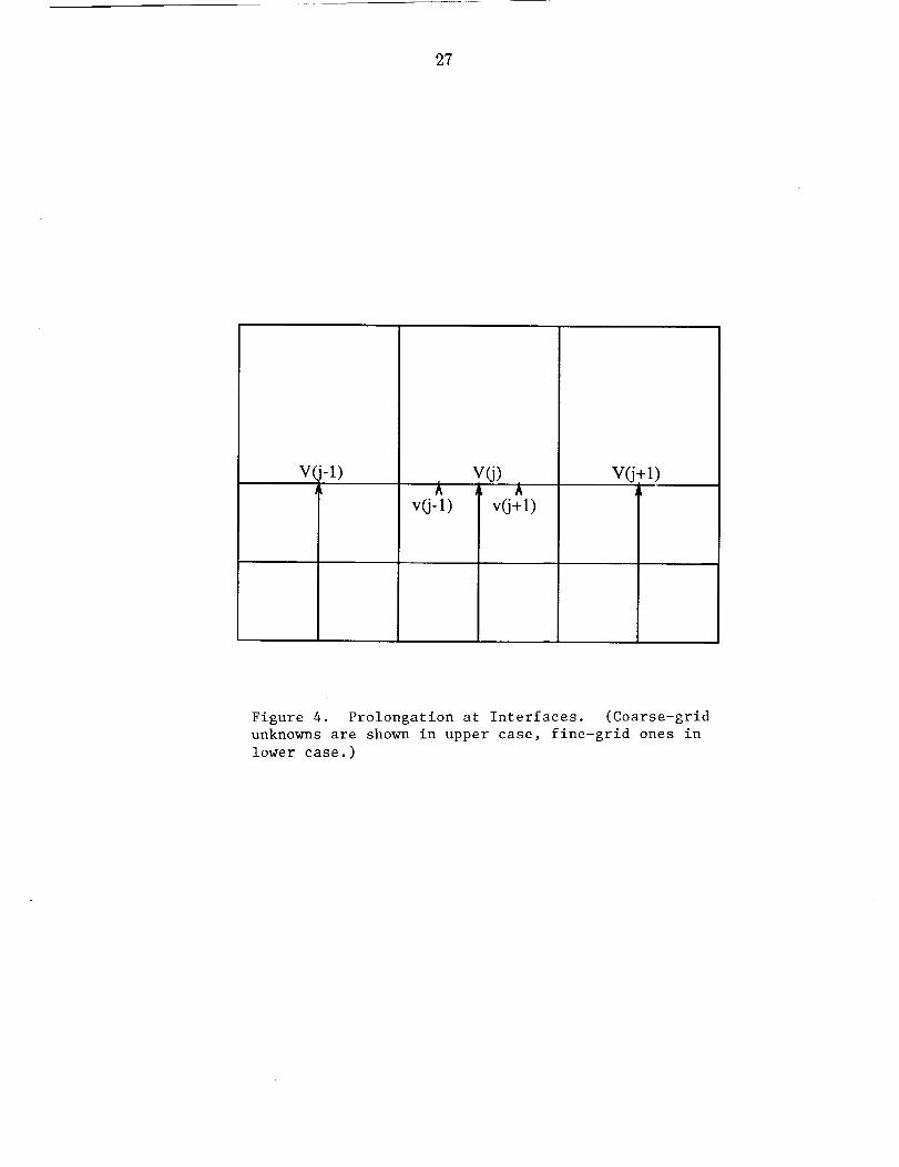
The primaryconsiderationis that thereis no solutionto the discreteequationsunlessdiscretemassis conserved. If we consider the flux across the (horizontal) interface, we require

2hV(j) = hv(j - 1)+ hv(j + 1),

where we have assumed that the fine grid size is h and that the nomenclature is as defined in Fig-

ure 4. This requirement is automatically satisfied by our standard restriction operation. However,

normal linear prolongation does not have this property. We have modified our prolongation

operator so that mass is conserved by this operator as well. We define the fine-grid neighbors of a

coarse-grid velocity by

and

v(j + 1) = V(j)+(V(j + 1)- V(j - 1))/8,

v(j - 1) = v(j)-(vo" + I)-V(j - 1))is.

These expressions are formally second-order accurate, and insure satisfaction of the continuity

equation across the interface. It is interesting to note that there arc no interpolation formulae

based on Lagrange polynomials that satisfy the discrete conservation property and that have order

higher than two.

The other aspect of the interface treatment is its effect on accuracy. Taking finite differences

of values obtained by interpolation is, in general, rather suspect. This is exactly what we do,

since the momentum equation at the interface involves differences of "dummy variables"

obtained by interpolation. One can show that with the linear interpolation our treatment of advec-

tion terms is first-order accurate at interfaces, while the treatment of viscosity terms is zeroth-

order accurate. Global truncation order is ordinarily one order of accuracy better, implying global

second-order accuracy for advection-dominated problems, but only first-order accuracy when

viscosity terms dominate.

Quadratic interpolation improves accuracy by one power of h, giving consistent treatment

of viscosity terms as well at interfaces. Thus, with quadratic interpolation, we can expect

second-order global accuracy, even when viscosity terms dominate, assuming there are only a

bounded number of interfaces in the domain. Even in the case where the number of interfaces

grows without bound, advection-dominated problems remain second-order accurate. All of this

suggests that the quadratic interpolation is superior, in practice, one sees relatively little

difference. The reason seems to be that for the advection-dominated problems considered, treat-

ment of viscosity terms is relatively unimportant. The simple linear interpolation scheme already

gives global second-order accuracy in most cases of interest and was used in most of our experi-

ments, since it is computationally more efficient. However, it is important to note that our uni-

form grid calculations are second-order accurate. Since our adaptive calculations are substantially

more accurate for a given computational cost, the issue of formal truncation error is moot.

9

7. Data Structures and Related Issues

From the outset of this work we adopted a refinement strategy that would allow any qua-

drant of any patch to be refined if it satisfied some criterion. When a quadrant is refine, each mass

control volume is divided into four, so that our fundamental data objects remain identical, even

though they have different mesh spacing and are associated with a different level in the grid

hierarchy. The entire patch structure that we generate is described by a quad tree.

Multigrid algorithms for nonlinear PDEs (full approximation storage schemes) calculate a

quantity known as the defect as an integral part of the iteration strategy. One definition is

which may be thought of as an approximation to the truncation error on the coarse grid. Other

investigators have used simpler error estimators based on (say) velocity gradients or curvature;

however, we prefer to use the defect, since it does not bias particular terms in the differential

equation.

Throughout this paper we have refined any quadrant that satisfies

[%_t ] quadrant>

where nVis is the number of quadrants that are visible (i.e., unrefined). Normally, we take

power = 1.0. However, this criterion is not crucial to our algorithm, and other criteria can be

substituted with minimal effort.

In addition to this criterion, two other mechanisms are used to control refinement. To

ensure that our grid ratio does not grow unreasonably, we force a refinement if the ratio is

(locally) greater than two. Moreover, in the immediate neighborhood of a re-entrant comer, if we

subdivide one quadrant that touches the comer, then we refine all three quadrants.

A number of data structures are required to support the various numerical processes that

have to be performed during our iterations. The proper design of these data structures enables

reasonably simple implementation of each of the numerical operations, even though the arrange-

ment of the data is now more complex. Typical lists of patch descriptors include the following:

• The NEXT patch at level N. (Linking the patches on each level this way allows all opera-

tions to be done by list traversal, rather than by a recursive tree walk.)

• The NEIGHBORS of each patch (simplifying data exchange during relaxation and interpo-

lation operations).

10

• Theidentifiersof thechildrenof eachpatch(KIDS)(necessaryfor prolongation).

• TheAUNTS (neighbors of the parents) of each patch (required for restriction).

Boundary conditions and geometric descriptors are also maintained for each patch, enabling

us, in principle, to handle curved boundaries or stretched meshes for resolution of boundary

layers.

With this information, the basic numerical operations can be implemented as loops going

along all the patches in a particular grid level. A typical code fragment could be

ID = LevPt(N)

DO 1 = 1,LevCnt(N)

Num_Op( Patch( ID ),Patc h(Kid( ID )))

119 = Next(ID)

ENDDO

! First patch on Level N

! All patches on Level N

f Perform numerical process

.t Next patch at this level

where NumOp is one of smoothing, prolongation, restriction, exchange of edge data, or applica-

tion of boundary conditions. It is clear that the normal multigrid cycling controls determine the

invocation of these code fragments.

The natural order is to process patches in the order of their creation (which determines their

place in the list). All processes (except smoothing) are independent of the ordering of the points.

Experiments have shown that the smoothing rate of our relaxation process is insensitive to the

ordering.

The aspect ratio of all cells remains constant throughout the refinement process. Of course,

grids built of rectangles can easily be used by appropriate definition of the original grid. How-

ever, the smoothing rate degrades if the aspect ratio is very different from unity. We are consider-

ing using line relaxation to avoid this effect, but some kind of patch sorting is required before this

strategy can be impIemented.

8. Numerical Results

We wish to focus attention on three main points. First, the rate of convergence and accu-

racy that we achieve on our automatically adapted grids must be comparable with our standard

calculations. Second, our local truncation error estimate 1_1 , w_ic_ weuse to controlmultigrid

our local refinement strategies, must give us reasonable patterns. Third, the accuracy we achieve

must be comparable with that obtained by other benchmarks. Additionally, we shall discuss

briefly our interface treatment and demonstrate the geometric flexibility of the algorithm. How-

ever, we have not attempted to develop optimal strategies for all aspects of this work, but rather to

validate the basic components.

11

8.1 The Driven-Cavity Problem

The first example we consider is the driven-cavity problem. This widely known problem is

well documented in the literature. We have chosen this problem because it is geometrically sim-

ple and the solution is well understood. However, the presence of singularities in the solution

clearly is going to cause any adaptive code difficulties. This fact should be borne in mind when

considering these results.

The problem domain is a unit square, and the flow is driven by specifying u = 1 and v = 0

on the top wall. On the other walls, we specify u = v = 0. There are singularities in the horizon-

tal velocity in the top comers of the domain.

Table l(a). Effect of Different Interface Treatments with Re = 1,

Fixed Refinement Patterns, and First-Order Boundary Treatment

(timings on a Sun/3 with Weitek floating-point accelerator)

Re = 1.0 Linear Interface Quadratic Interface

Grid

16

16+5

16+5+5

16+5+5+5

16+5+5+5+5

512x512

P_tq

6.O9874

5.98808

5.967O3

5.94360

5.93034

5.8719O

error Of # T (see)

2.27(-1) .41 18 4

1.16(-1) .44 19 ll

9.51(-2) .46 21 24

7.17(-2) .45 22 50

5.84(-2) .46 24 107

_W

6.09874

5.96708

5.90704

5.87535

5.86125

5.87190

error Of

2.27(-1) .41

9.52(-2) .46

3.51(-2) .46

3.45(-3) .44

1.06(-2) .45

#

18

19

21

22

24

T (see)

4

11

24

51

110

f

12

Table 1(b). Effect of Different Interface Treatments with Re = 400,

Fixed Refinement Patterns, and First-Order Boundary Treatment

Re = 400

Grid

64x64

64 x 64+5

64 x 64+10

128 x 128

128 x 128+5

128 x 128+10

64 x 64+5+5

Linear Interface

2.549(-2)

2.503(-2)

2.503(-2)

2.479(-2)

2.491(-2)

2.491(-2)

2.515(-2)

Quadratic interface

Error

5.2(-4)

0.6(-4)

0.6(-4)

1.8(-4)

0.6(-4)

0.6(-4)

1.8(-4)

#

15

12

11

11

10

9

2.549(-2)

2.493(-2)

2.500(-2)

2.479(-2)

2.479(-2)

2.487(-2)

2,493(-2)

Error

5.2(-4)

0.4(-4)

0.3(-4)

1.8(-4)

1.8(-4)

1.0(-4)

0.4(-4)

#

15

12

12

11

11

10

11

Notes: 64 x 64 and 128 x 128 denote uniform-grid calculations.

64 x 64+5 has the five rows of mass control volumes at the top of the domain subdivided

(each cell becoming four finer cells).

64 x 64+5+5 has the top five rows of cells of the 64 x 64+5 grid subdivided.

Other definitions are obvious generalizations of this.

First, we consider the effect of the interface treatment on the accuracy of the solution.

Tables l(a) and l(b) show the wall shear stress and the associated errors at the midpoint of the

wall. The wall shear value shown in the tables was calculated by using third-order, one-sided

interpolation. The error was measured by taking the value calculated on a 512 x 512 grid as

exact. (The discretized equations used a one-sided, first-order approximation for the wall shear,

for simplicity.) For the purposes of this comparison only, we have forced the refinement patterns.

The grid refinements, explained in the table notes, were chosen to allow reasonable representa-

tions of the boundary layer.

From these tests (and others at even higher Reynolds numbers), we deduced that second-

ordcr interpolation was adequate for our fully adaptive strategy. (As we expected, the quadratic

formulae are somewhat more accurate, but the gains do not seem to justify the additional com-

plexity.) Clearly, this approach differs from that described in, for example, reference [6]. Our

goal is to introduce refinements that efficiently reduce the errors associated with the existing grid

calculations, rather than to maintain a particular order of truncation error. Formal truncation error

analysis and its relationship to actual errors is a complex issue in this context. We are not claim-

ing that our adaptive discretization is second order. However, our uniform grid calculations are,

in general, second order. Throughout this section we compare the adaptive and the uniform (i.e.,

second-order) strategies on the basis of speed, accuracy, and storage.

Table l(c) shows the performance of the fully automatic adaptive code, relative to uniform

grid calculations, The Reynolds number is 400. The errors have been estimated by considering

13

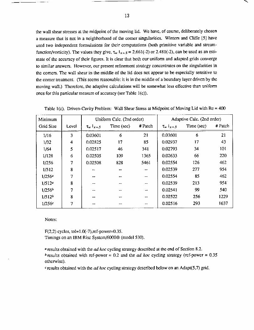
thewall shearstressesatthemidpointof themovinglid. Wehave,of course,deliberatelychosena measurethatis not in aneighborhoodof thecomersingularities.WintersandCliffe [5] haveusedtwo independentformulationsfor their computations(bothprimitivevariableandstream-function/vorticity).Thevaluestheygive,xw I;,=.5 = 2.661(-2) or 2.481(-2), can be used as an esti-

mate of the accuracy of their figures. It is clear that both our uniform and adapted grids converge

to similar answers. However, our present refinement strategy concentrates on the singularities in

the comers. The wall shear in the middle of the lid does not appear to be especially sensitive to

the comer treatment. (This seems reasonable: it is in the middle of a boundary layer driven by the

moving wall.) Therefore, the adaptive calculations will be somewhat less effective than uniform

ones for this particular measure of accuracy (see Table l(c)).

Table l(c). Driven-Cavity Problem: Wall Shear Stress at Midpoint of Moving Lid with Re = 400

Minimum Uniform Calc. (2nd order) Adaptive Calc. (2nd order)

Grid Size Level "c_,Ix =.5 Time (sec) # Patch "cwIx =.5 Time (sec) # Patch

1/16

1/32

1/64

1/128

1/256

1/512

1/256 a

1/512 a

1/256 b

11512 t,

1/256 c

3

4

5

6

7

8

7

8

7

8

7

0.03601 6 21

0.02825 17 85

0.02517 46 341

0.02505 109 1365

0.02508 828 5461

0.03601 6 21

0.02937 17 43

0.02793 34 101

0.02633 66 220

0.02554 126 462

0.02539 277 954

0.02554 85 462

0.02539 213 954

0.02541 99 540

0.02522 256 1229

0.02516 293 1637

Notes:

F(2,2) cycles, tol= 1.0(-7),ref-power=-0.35.

Timings on an IBM Risc System/6000® (model 530).

a results obtained with the ad hoc cycling strategy described at the end of Section 8.2.

b results obtained with ref-power = 0.2 and the ad hoc cycling strategy (ref-power = 0.35

otherwise).

results obtained with the ad hoc cycling strategy described below on an Adapt(5,7) grid.

14

Theverticalvelocityextremaat thehorizontalmid-planeareanalternativeerrormeasure.In Table l(d) wecompareadaptiveanduniformcalculationson thebasisof thesequantities.Again,weseetheimportanceof therefinementstrategy.However,theAdapt(5,7)calculationhasaccuracycomparablewith theuniformseven-levelcalculation(atleastfor theminimumverticalvelocity)with considerablesavingsin cpu time andcomputerstorage.Physically,onecouldarguethatthedownturnin thehorizontalboundarylayeris causedby thepressuremaximumatthetopright-handcomerof thedomain.Our adaptivestrategyhascapturedthisdownturnandhasalsorefmedthemeshdownwards,followingthis "jet." In Figure5, weshowaseven-leveladaptivegrid andtheresultingflow visualizationconsistingof the levelcurvesfor thestreamfunction.

Tablel(d). Driven-CavityProblem:VelocityExtremaattheHorizontalMidplane

Minimum MidplaneY=0.5Grid Size Level Comment Vm_, Vmax Time (sec) # Patch

1/16

1/32

1/64

1/128

1/256

1/256 a

1/256 a

3

4

5

6

7

7

7

Uniform

Uniform

Uniform

Uniform

Uniform

Adapt(3,7)

-0.2931 0.1801

-0.3923 0.2529

-0.4396 0.2946

-0.4518 0.3021

-0.4534 0.3033

-0.4388 0.2852

Adapt(5,7) -0.4523 0.3020

6 21

17 85

46 341

109 1365

828 5461

85 462

293 1637

Notes:

Validation and serial performance for the adaptive code: vertical velocity extrema across the hor-izontal midplane.Adapt(n,m) defines a calculation with n levels of uniform refinement and then adaptiverefinement up to level m. (In this table we had ref-power = 0.35.)Timings on an IBM Risc System/6000® (model 530).

a results obtained with the ad hoc cycling strategy described at the end of Section 8.2.

Table l(e) shows the rates of convergence for the driven-cavity problem on uniform and

adapted grids. As is typical of multigrid algorithms on nonlinear problems, the convergence rate

varies somewhat as the number of levels increases but remains bounded well away from one uni-

formly in the number of grid levels.

Of greater significance, we note that the convergence rates achieved on the adapted meshes

are comparable to the uniform grid rates. One would not necessarily expect this result on theoret-

ical grounds; ii _nounts-to a pleasantsurpfise_ 'i_e-c_culatior_ here are terminated on each grid

when the norm of the residual is less than 10.0(-07). The reduction factors given in the table are

thefinal reduction factors; in some cases they have not reached their asymptotic values.

15

Eachof ourtestcasescontainssomeformof singularity(orsingularities).Wearenot treat-ing thesein anyspecialfashion;theyareautomaticallyhandledby our refinementstrategy.Ingeneral,for complexflows, it is impossibleto predictall possiblesingularities;therefore,methodsthatrelyonaccurateandspecialtreatmentof theseregionsarenotsufficientlyflexible.Oursolutionsareobviouslygoingto be poor in small neighborhoods of the singularities, but this

effect is local; moreover, careful mesh grading allows a solution to be obtained without degrada-

tion of the order of accuracy (see, for example, [3] and [8]).

Table 1(e). Driven-Cavity Problem:

Rate of Convergence on Adaptive and Nonadaptive Grids, with Re = 400

Grid

Level

2

3

4

5

6

7

8

Uniform Calculation (2nd) Adapted Calculation (2nd)

Total Fine No. Total Fine No.

Pats. Pats. Cycles 9/" Pats. Pats. Cycles

5 4 23 .51

21 16 20 .47

85 64 24 .52

341 256 22 .55

1365 1024 15 .31

5461 4096 20 .62

5 4 23 .51

21 16 20 .47

43 22 19 .42

101 52 17 .23

220 102 16 .47

462 169 15 .42

954 321 17 .52

Notes:

F(2,2) cycles, tol. = 1.0(-7), ref-power = 0.35.

Second-order boundary conditions.

8.2 The Flow over a Backward-Facing Step Problem

The flow over a backward-facing step is another geometrically simple and well-documented

problem. As is usual, we have specified a parabolic inlet profile (fully developed flow), and we

have fully developed outlet conditions. No slip conditions are imposed at all walls. In this

configuration, we calculate the flow upstream of the step, thereby solving for the flow around the

step and not ignoring the singularity at the comer. In contrast to [15], important features of this

flow are the recirculation zone behind the step and the velocity profiles downstream of the step.

In Table 2(a) we give the convergence rates for the uniform-grid and adapted-grid calcula-

tions. Little degradation is observed in the adapted-grid computations, despite the complexity of

the problem domain. However, the uniform-grid calculations at level 3 converge more quickly

!

16

because the diffusion terms become more important than the convective terms as the mesh-size

decreases. This effect is not seen on the adaptive calculations because some parts of the coarser

grid remain visible.

Table 2(a). Rate of Convergence for the Backward-Facing Step Problem:

Uniform and Adaptive Calculations

Grid

Level

2

3

4

9

10

Uniform Calculation

Total Fine No.

Pats. Pats. Cycles p/'

180 144 16 .52

756 576 9 .24

II tl

Adapted Calculation

Total Fine No.

Pats. Pats. Cycles 9f

180 144 16 .52

240 60 11 .41

391 114 10 .40

525 19 14 .42

544 19 15 .42

Notes: F(2,2) cycles with Re = 150, power = 2.0, and tol. = 10.0(-6).

17

Table2(b).ResultsfortheBackward-FacingStep:UniformandAdaptiveCalculationsandBenchmark

Uma_

1.6 step-ht

4.0 step-ht

Umin

1.6 step-ht

4.0 step-ht

Vmax

1.6 step-ht

4.0 step-ht

Vmin

1.6 step-ht

4.0 step-ht

No. patches

Time (sec)

Total Time (sec)

Velocity

Cliffe

0.904

0.725

0.010

0.0

(2,2) (3,3)

0.897 0.903

0.725 0.722

-0.103 -0.103

-0.036 -0.047

0.010 0.010

0.0 0.0

-0.068 -0.070

-0.077 -0.087

180 756

73 77

73 77

(2,4) (2,10)

0.906 0.905

0.726 0.725

-0.102 -0.101

-0.039 -0.038

0.010 0.010

0.0 0.0

-0.071 -0.071

-0.089 -0.089

391 544

113 --

278 --

Notes: (2,2): uniform 2-level calculation with mesh size = step-height/8.

(3,3): uniform 3-level calculation with mesh size = step-height/16.

(2,N): adapted calculation with maximum mesh size = step-height/8 and minimum mesh size"

= step-height/2(N+D.

To assess the accuracy of our approach, we have included uniform, adapted, and benchmark

solutions; see Table 2(b). The benchmark solutions were taken from reference [14]. Clearly, all

the sets of calculations are in agreement. Moreover, the adaptive calculations with two levels of

18

automaticrefinement(shownas(2,4)in thetable)useonlyhalfthestorageof theuniform3-levelcalculationsfor comparableaccuracy.A weaksingularityin theneighborhoodof thecomerinhi-bits furtherimprovementof thesolutionwithourcurrentrefinementstrategy.However,thereisno degradation in the solution if we allow more refinement (we allowed a further six levels).

Therefore, our interface treatment is reasonable.

We show two sets of flow visualizations and refinement patterns for this configuration. The

first set (Figure 6(a)) was obtained by using a naive treatment of the inlet and first-order treat-

ments of the walls. The code has automatically detected this and refined the pattem in the areas

where the approximation is poor. When we improved these two aspects so that we had a con-

sistently second-order treatment throughout the domain, we obtained the refinement patterns

shown in Figure 6(b) (the values used in Table 2(b) used the improved treatments).

Our coarsest-grid treatment simply consists of many sweeps. In many circumstances this is

adequate. However, in cases where there are many patches on the first grid, it is obvious that

various forms of acceleration could be used. At present, these have not been implemented since

the benefits are probably marginal. Moreover, we can decrease this effect by making minor

modifications to the multigrid cycling strategy.

Another factor that affects our adaptive timings is that, at present, we solve a sequence of

flow problems so that we have reliable error estimates that are "uncontaminated" by insufficient

numerical convergence; these are the basis of our refinement strategy. It may be possible to avoid

this _equential procedure by doing the refinement and solution concurrently (in some sense).

However, we have avoided this strategy in the present study since the convergence errors confuse

the refinement patterns. The only attempt we have made to address this issue is the ad hoe

strategy referred to in the tables. Here we do the following: when performing an Adapt(n ,m) cal-

culation (uniform refinement on n grids, then adaptive refinement up to level m), we reset the

cycling tolerance to its square root until we have completed the preliminary problems and we

have an adapted m-level grid. We then solve the m-level problem to the full tolerance. This

strategy decreases the set-up time, without significantly changing the final adapted grid or the

computed solution. For two of the geometries in this paper, this strategy is quite effective. How-

ever, for the backward-facing step geometry we were able to reduce the time for the Adapt (2,4)

calculation only to 180 seconds. The coarsest-grid effects still dominate when we have such a

small number of levels.

8.3 The Sudden Expansion�Contraction Geometry

The third example is new. it consists of a sudden expansion/contraction and was chosen to

show the flexibility of our approach. (The choice was also tempered by the desire to have an

intuitive feeling for the correcmess of our results.) The geometry is shown in Figure 7. At the

19

extremeleft,wespecifya parabolicinletprofilefor thehorizontalvelocity(andv = 0). On the

right we specify fully developed flow conditions: v = 0 and _xu = 0. Everywhere else we have

u = v = 0. This flow has four re-entrant comers. An interesting quantity is the flux across the

"entrance" to the expansions in the domain.

The rates of convergence (Table 3) agree with the results of the preceding sections: adap-

tivity does not slow down convergence. Again we see the uniform-grid calculations improving as

the mesh becomes finer, because the elliptic terms become dominant; but this effect is not seen in

the adaptive calculations, because sections of the coarse grids remain "visible" and limit the rate

of convergence. The flow visualization (Figure 7) shows that we are obtaining qualitatively rea-

sonable results. There are two shear-driven recirculation cells formed behind the steps. The

streamlines seem to be quite reasonable.

The streamlines shown in the figures were calculated by integrating over the adapted grid.

The use of this adapted mesh was necessary because the conservation equation is satisfied here.

We used Gaussian quadrature, modified to capture the compound grid automatically. Techniques

that ignored this fact gave disappointing results.

One quantity of interest is the transport from the main channel into the two expansions. We

have measured this by looking at the vertical velocity extrema along the "continuation" line

across the top of the channel. Both the uniform and adaptive calculations converge to the same

values; however, when the ad hoc cycling strategy is used, the adaptive calculations are faster and

use less memory.

20

Table3. SuddenExpansion/ContractionGeometry:Rateof ConvergenceandVerticalVelocityExtrema

Uniform Calculation Adaptive Calculation

Minimum Vert. Velocity Time No. No. Vert. Velocity Time (see) No. No.

Grid Size Max Min (sec) Patches Cycles Max Min Item Cumul. Patches Cycles

1/8

1/16

1/32

1/64

1/128

1/64 _

1/128 a

0.0212 -0.073 6 25 11

0.0224 -.088 9 105 9

0.0233 -.092 22 425 8

0.0254 -.099 72 1705 8

0.0212 -0.073 6 6 25 11

0.0230 -0.090 11 16 55 14

0.0243 -0.094 18 34 I11 12

0.0254 -0.100 27 61 185 14

0.0262 -0.100 44 106 283 14

0.0257 -0.100 31 46 186 14

0.0262 -0.100 44 69 284 14

Notes:

Re = 50, F(2,2) cycles, tol=l.0(-7), ref-power=-1.0.

Timings on an IBM Risc System/6000® (model 530).

a Results obtained with the ad hoc cycling strategy.

9. Discussion

There are three reasons why one is interested in automatic adaptive gridding strategies:

speed, storage, and reliability of the solution. The first item has been dealt with earlier.

The issue of storage is fairly simple, and we have been able to achieve significant savings in

all cases of interest. Here we simply add the comment that, in three-dimensional problems, the

question of efficient storage utilization is significantly more important and the benefits from adap-

tive gridding correspondingly greater.

The issue of reliability of the computed solution is complex. Our present refinement

strategy is somewhat ad hoc, and a detailed study of refinement strategies is beyond the scope of

this paper. However, our examples illustrate three types of error: (1) those induced by some type

of singularity, (2) those caused by comparatively poor numerical treatments (e.g., low-order

boundary formulae), and (3) those caused by insufficient grid resolution. The best that one can

hope to do in the presence of singularities is to treat them sufficiently well that their effect is local

21

(unless one uses some semianalytic approach). Our code does this. Moreover, the other two

effects are detected and automatically reduced by our refinement strategy until the errors are dom-

inated by singularity effects.

The question of how a numerical solution varies with respect to "small" changes in the grid

is not well understood, nor is the global effect of singularities in the domain. Attention must be

given to these points before we can achieve "full reliability." However, it is interesting to note

that the problems with singularities are not restricted to error estimators based on the defect (or

the local truncation error). Richardson extrapolation techniques and simpler gradient estimators

can have the same problems.

Throughout this work we have measured errors by estimating a continuous solution and

defining errors with respect to this. We have the following equation:

Lh [eh ] ='_ t,

where e h is the discrete error. Since the equation is linear, it can be solved with comparatively

little extra work, given that the operator and the gridding are already defined. This approach

offers possibilities of improving our refinement strategies. However, e h may contain nonlocal

errors, thereby complicating its use in a refinement strategy.

10. Conclusions

As is customary with this type of work, we have demonstrated the effectiveness and accu-

racy of our techniques by considering a few, well-known model problems.

We have shown that the rate of convergence we observe for the adaptive calculations does

not degrade significantly compared to the uniform ones. Our estimate of the local truncation error

(x/_) gives us qualitatively correct refinement patterns, which are capable of detecting deficiencies

in the numerical treatment as well as in the grid. The accuracy of our results is comparable with

that of other benchmarks for both the uniform and the adaptive calculations. Our current adaptive

strategy will deal with all three classes of error. However, it continues to "home in" on singulari-

ties, even though this is not always an optimal strategy.

Additionally, we have shown that the interpolation that we use at interfaces is good and that

we are easily able to handle a range of geometries. For some of the cases we have considered, we

have been able to achieve significant gains in speed and storage compared to uniform grid calcu-

lations. However, we have shown that this is not always the case.

f

22

11. Future Work

In the current work we showed that we can separate the three components--the multigrid

algorithm, the adaptive strategy, and the numerical approximations--as was our design goal. Now

that we have done this, we can modify and improve each of these aspects separately. In particu-

lar, we are looking at efficient ways to improve the generality, scope, and accuracy of the algo-

rithrn. We are also focusing our attention on parallelization issues. A shared-memory version of

this code is running, and we are about to look at implementation on scalable distributed-memory

architectures, such as the Intel® Touchstone DELTA system.

Acknowledgments

This work benefited from several fruitful discussions with Dr. N. W. Wilkes of Harwell

Laboratory, England, who provided important assistance with our boundary treatments. We are

happy to acknowledge the assistance of Lisbeth Skodvin, Bergen Scientific Centre, for help with

the visualizations used in this paper.

IBM and Risc System/6000 are trademarks of IBM Corporation. Intel is a trademark of

Intel Corporation.

References

[1] C.P. Thompson, G. K. Leaf, and S. P. Vanka, Application of a multigrid method to a

buoyancy-induced flow problem, in Multigrid Methods Theory, Applications, and Super-

computing, S. F. McCormick (Ed.), pp. 605-630, Marcel Dekker, New York, 1988.

[2] H.C. Ku, R. S. Hirsh, and T. D. Taylor, A pseudospectral method for solution of the three-

dimensional incompressible Navier-Stokes equations, J. Comp. Phys. Vol. 70, pp. 439-462,

1987.

[3] G. Strang and G. J. Fix, An analysis of the finite element method, Prentice-Hall, Englewood

Cliffs, 1973.

A. Brandt and N. Dinar, Multigrid solutions to elliptic flow problems, in Numerical

Methods for PDEs, S. V. Parter (Ed.), pp. 53-147, Academic Press, New York, 1979.

K. H. Winters and K. A. Cliffe, A finite element study driven laminar flow in a square cav-

ity, AERE - R 9444, AERE Hal-well, UK, 1979.

G. Chesshire and W. D. Henshaw, Composite overlapping meshes for the solution of partial

differential equations, J. Comp. Phys. Vol. 90, No. 1, pp.1-64,1990.

S. P. Vanka, Block-implicit multigrid solution of Navier-Stokes equations in primitive vari-

ables, J. Comp. Phys. Vol. 65, No. 1, pp.138-158,1986.

[4]

[51

[6]

[7]

23

[8] L. Fuchs,A localmeshrefinementtechniquefor incompressibleflows,Computers and

Fluids, Vol. 14, No. 1, pp. 69-81, 1986.

[9] A. Brandt, Multigrid Techniques: 1984 Guide with Applications to Fluid Dynamics, Com-

putational Fluid Dynamics, Lecture Series 1984-04, yon Karman Institute, Belgium, 1984.

[10] K. Stueben and U. Trottenberg, Multigrid Methods, Fundamental Algorithms, Model Prob-

lem Analysis and Applications, Multigrid Methods, Lecture Notes in Mathematics, Vol.

960, Springer Verlag, Berlin, 1982.

[11] D. Bai and A. Brandt. Local mesh refinement multilevel techniques SIAMJ. Sci. Stat. Corn-

put. Vol. 8, pp. 109-134, 1987.

[12] S. McCormick and J. W. Thomas. The fast adaptive composite grid (FAC) method for

elliptic equations, Math. Comp. Vol. 46, pp. 439-459, 1986.

[13] N. S. Wilkes and C. P. Thompson. An evaluation of higher-order upwind differencing for

elliptic flow problems, in Numerical Methods for Laminar and Turbulent Flow, C. Taylor,

J. A. Johhnson and W. R. Smith (Eds.), pp. 248-257, Pineridge Press, 1983.

[14] K. A. Cliffe, I. P. Jones, J. Porter, C. P. Thompson and N. S. Wilkes. Laminar flow over a

backward facing step: Solution to a test problem, in Analysis of Laminar Flow over a

Backward-Facing Step: A GAMM Workshop, K. Morgan, J. Periaux, F. Thomasset (Eds.),

pp. 140-161, Friedr. Vieweg and Sohn, 1983.

[15] M. C. Thompson and J. H. Ferziger, An adaptive multigrid technique for the incompressible

Navier-Stokes equations, J. Comp. Phys. Vol. 82, No. 1, pp. 94-121, 1989.

[16] C.P. Thompson, W. R. Cowell, and G. K. Leaf. On the parallelization of an adaptive mul-

tigrid algorithm for a class of flow problems, preprint MCS-P205-0191, Mathematics and

Computer Science Division, Argonne National Laboratory, 1991.

[17] L. P. Hackman, G. D. Raithby, and A. B. Strong, Numerical predictions of flows over

backward-facing steps, Int. J. Num. Meth. Fluids, Vol. 4, pp. 711-724, 1984.

24

u=l, v=O

U=v=O U=v=O

u=v=O

Figure l(a). Driven Cavity:

Solution Domain and Boundary

Conditions

i VT

PO

$(v)

U

Figure l(b). Staggered Grid: Location

of Variables. Bracketed variables are

associated with adjacent cells.

25

i i

O

O

_,- O

i

_- O

- w

"- O

. w

t | ti I

- I P'_ I _

_w m _

I l

! i

I I

I II -i I

0

(a) One grid level, one patch.

(b) Two grid levels, three patches.

"- O ":

m_

! i I

I "_J I

I i

I f%

I _.J

I tI I

0

(c) Three grid levels, four patches.

Figure 2. Composite Grids at Each Level

26

V v v

U P

V

u p u p

v v

up up

V V

U

U

Figure 3(a). The Canonic Problem: One Coarse-Grid Patch Interfacing

with Four Fine-Grid Patches. This tiling is sufficient to generate

all configurations of interest. We show the location of "genuine"

unknowns on the compound grid. At these locations we solve approxi-

mations of the differential equations. (Coarse-grid variables are in

upper case, fine-grid ones in lower case.)

v V!

I

I

,u pO

I

l VL .... ----,

I

I

]

,u pI

I

l V

U P

V

Figure 3(b). The Canonic Problem Modified to Show the Dummy Unknowns

Introduced for Computational Convenience. The variables shown here

are not unknowns in our system of equations but dummy variables that

are introduced for convenience. Special, additional equations are

introduced for them. (Coarse-grid variables are in upper case, fine-

grid ones in lower case.)

27

V(j-1)A

v(j-1)

vG)A

v(j+l)

V(j+I)

Figure 4. Prolongation at Interfaces. (Coarse-grid

unknowns are shown in upper case, fine-grid ones in

lower case.)

28

J

i i i

i

r

i I I " --

7r--L-_---4• II

t -rI

Figure 5. The Driven Cavity Problem: Flow visualization, an adapted grid and problem

definition. On the top wall we drive the flow by specifying u = 1 (and v = 0). On the other

walls we have u = v = 0. There are singularities in the horizontal velocity in the two top

comers of the domain.

29

p

(a)

Figure 6. The Backward-Facing Step Problem: Flow visualization, an adapted grid and

problem definition.

(a) First-order boundary conditions and standard inlct treatment,

(b) Second-order boundary conditions and modified inlet treatment.

At the extreme left we specify a parabolic inlet profile for the horizontal velocity (and

v = 0). On the right we specify fully developed flow conditions: v = 0 and _xu = 0. On all

other boundaries we have u = v = 0. Notice that we are solving the flow around the step

and not ignoring the singularity at the comer. This is a significantly more difficult problem

than considering a rectangular domain only.

30

÷

Figure 7. The Cross Geometry: Flow visualization, an adapted grid, and problem definition.

At the extreme left we specify a parabolic inlet profile for the horizontal velocity (and v = 0). On

the right we specify fully developed flow conditions: v = 0 and _xu = 0. On all other boundaries

we have u = v = 0. This flow has four re-entrant comers. An interesting quantity is the flux

across the "entrance" to the expansions in the domain. Pe_ velocities are shown in Table 3.

Report Documentation Page

t. Report No. 2. Government Accession No. 3, Recipient's Catalog No.NASA CR- 187595

ICASE Report No. 91-36

5. Report Date

June 1991

4. Title and Subtitle

A DYNAMICALLY ADAPTIVE MULTIGRID ALGORITHM FOR THE

INCOMPRESSIBLE NAVIER-STOKES EQUATIONS -- VALIDATION

AND MODEL PROBLEMS

7. Author(s)

C. P. Thompson

G. K. Leaf

J. Van Rosendale

9. PerformingOrganization Name and AddressInstitute for Computer Applications in Science

and Engineering

Mail Stop 132C, NASA Langley Research Center

Hampton, VA 23665-5225

12. Spon_ring Agency Name and Addre_National Aeronautics and Space Administration

Langley Research Center

Hampton, VA 23665-5225

6. PerformingOrganization Code

8. PerformingOrganization Report No.

91-36

10. Work Unit No.

505-90-52-01

11. Contract or Grant No.

NASI-18605

13. Type of Report and Period Covered

Contractor Report

14, Sponsoring&gency Code

15. Supplementaw Notes

Langley Technical Monitor:

Michael F. Card

Submitted to J. Applied Numerical

Mathematics

Final Report

16. Abstract

We describe an algorithm for the solution of the laminar, incompressible Navier-Stokes equations. The basic

algorithm is a multigrid method based on a robust, box-based smoothing step. Its most important feature is the

incorporation of automatic, dynamic mesh refinement. Using an approximation to the local truncation error to

control the refinement, we use a form of domain decomposition to introduce patches of finer grid wherever they

are needed to ensure an accurate solution. This refinement strategy is completely local: regions that satisfy ourtolerance are unmodified, except when they must be refined to maintain reasonable mesh ratios. This locality has

the important consequence that boundary layers and other regions of sharp transition do not "steal" mesh pointsfrom surrounding regions of smooth flow, in contrast to moving mesh strategies where such "stealing" is inevitable.

Our algorithm supports generalized simple domains, that is, any domain defined by horizontal and vertical lines.This generality is a natural consequence of our domain decomposition approach. We base our program on a standard

staggered-grid formulation of the Navier-Stokes equations for robustness and efficiency. To ensure discrete mass

conservation, we have introduced special grid transfer operators at grid interfaces in the multigrid algorithm. Whilethese operators complicate the algorithm somewhat, our approach results in exact mass conservation and rapid

convergence.In this paper, we present results for three model problems: the driven-cavity, a backward-facing step, and

a sudden expansion/contraction. Our approach obtains convergence rates that are independent of grid size and

that compare favorably with other multigrid algorithms. We also compare the accuracy of our results with otherbenchmark results.

17. Key Wor_ (Suggest_ by Au_orls))

adaptive grids, incompressible flow

19. SecuriW Cla_if. (of this report)

Unclassified

NASA FORM lli2S OCT86

I

18. DistributionStatement

64 - Numerical Analysis

Unclassified - Unlimited

_. SecuriW Cla_if. (of this page}

Unclassified

21. No. of pages

32

22. Price

AO 3

NASA-Langley, 1991