Embed Size (px)
Citation preview

NAS-CR-149992 ) RESEARCH STUDY ON gt1PS N76-322-14DIGITAL CONTROLLER DESIGN Final Report(Systems Research Lab Champaign Ill)
2 -P C $5550 CSCL 22A Unclas G313 03490
I L [IT
V - 76
FINAL REPORT
RESEARCH STUDY ON IPS DIGITAL CONTROLLER DESIGN
B C KUO
C FOLKERTS
September 1 1976
Prepared for
NATIONAL AERONAUTICS AND SPACE ADMINISTRATION
GEORGE C MARSHALL SPACE FLIGHT CENTER
Under Contract NAS8-31570
DCN I-6-ED-02909(IF)
Systems Research Laboratory
P 0 Box 2277 Station A
Champaign Illinois 61820
TABLE OF CONTENTS
1 Analysis of the Continuous-Data Instrument Pointing System I
2 The Simplified Linear Digital IPS Control System 10
3 Analysis of Continuous-Data IPS Control System With Wire Cable Torque Nonlinearity 23
4 Analysis of the Digital IPS Control System With Wire Cable Torque Nonlinearity 33
5 Gross Quantization Error Study of the Digital IPS Control System 45
6 Describing Function Analysis of the Quantization Effects of the Digital IPS Control System 50
7 Digital Computer Simulation of the Digital IPS Control System With Quantization 66
8 Modeling of the Continuous-Data IPS Control System With Wire Cable Torque and Flex Pivot Nonlinearities 71
9 Describing Function of the Combined Wire Cable and Flex Pivot Nonlinearities 78
10 Modeling of the Solid Rolling Friction by the First-order Dahl Model 88
11 Describing Function of the First-order Dahl Model Solid RollingFriction 94
12 Modeling of the Solid Rolling Friction by the ith-order Dahl Model and the Describing Function 101
13 Digital Computer Simulation of the Continuous-Data Nonlinear Control System With Dahl Model 107 References 117
I Analysis of the Continuous-Data Instrument Pointing System
The objective of this chapter is to investigate the performance of
the simplified continuous-data model of the Instrument Pointing System
(IPS) Although the ultimate objective is to study the digital model
of the system knowledge on the performance of the continuous-data model
is important in the sense that the characteristics of the digital system
should approach those of the continuous-data system as the sampling period
approaches zero
The planar equations which describe the motion of the Space-lab using
Inside-Out Gimbal (IOG) for the pointing base are differential equations 1
of the fourteenth order A total of seven degrees of freedom are
represented by these equations Three of these degrees of freedom (Xs Zs
P ) belong to the orbitor and three degrees of freedom (Xm Zm Y) are
for the mount and the scientific instrument (SI) has one degree of freeshy
dom in 6
A simplified model of the IPS model is obtained by assuming that all
but motion about two of the seven degrees of freedom axes are negligible
The simplified IPS model consists of only the motion about the scientific
instrument axis c and the mount rotation T The block diagram of the
simplified linear IPS control system is shown in Figure 1-1
In this chapter we shall investigate only the performance of the
continuous-data IPS control system The signal flow graph of the
continuous-data IFPS control system in Figure 1-1 is shown in Figure 1-2
The characteristic equation of the continuous-data IPS is obtained
from Figure 1-2
A = (I - K4K6)s5 + (K2 + KIK 7 - KI K4K7)s4 + (K - KK4K7 + KK7 + KI K2K7) 3
0- Compensator
Compensator = I for rigid-body study
Figure T-1 Block diagram of simplified linear IPS control system
s-1 n fI
- -K
cu t ct s
-KK2
Figure 1-2 Signal flow graph of the simplified linear
continuous-data IPS control system
+ (KIK 7 - KK 4 K7 + KIK3K 7 + K0K2 K7)s 2 + (KIK 2 K7 + KoK3 K7)s K K3 K = 0
I-I)
The system parameters are
KO = 8 x i0 n-m
KI = 6 x 10⁴ n-msec
K = 00012528
K = 00036846
K = variable
K4 = o80059
K = 1079849
K6 = 11661
K = 00000926
Equation (1-1) is simplified to
5s + 16 704s4 + 22263s3 + (1706 + 27816 105K )s2
+ (411 + 1747 1O- 8 K )s + 513855 10- 8 KI = 0 (1-2)
The root locus plot of Eq (1-2)when KI varies is shown in Figure 1-3
It is of interest to notice that two of the root loci of the fifth-order
IPS control system are very close to the origin in the left-half of the
s-plane and these two loci are very insensitive to the variation of K-
The characteristic equation roots for various values of K are tabulated
in the following
KI ROOTS
0 0 -000314+jO13587 -83488+j123614
104 -00125 -000313984j0135873 -83426ojl23571
1O5 -01262 -00031342+j0135879 -828577+j123192
106 -138146 -00031398+jO135882 -765813+jill9457
____________ ________ ______________
--
--
centOwvqRAoPM(9P ] r ~NRL 0 fnw Nv-Yk SQUARE O010 10 THEINCH AS0702-10 4
- L c---- -4 - - -shy
i Q-2IIp 7 F
- - I ~ 17 - - - - -- --- w 1 m lz r - shy-
_ _ __ __o__o _ - -- _
---n --jo- - _ iI_ - sect- - --- j -- - - _
- - - - x l - ~ ~ j m- z - -- is l] n T
- -i - - - - -- - I L -4- - I - X-i- a shy- shy
i- wt -- -w 2 A -(D - - m- I - ______I _____ _ I-__ ___ ____ ____
(D - -I------=- -- j
- -+ - - I 1l - - - ---In- - - --- _- _ - shy _- - _ I
L a- - - ___0 __ - - -c -2 1-+J -I - A -- - -- __- 4 -
-
0-- - -I -shy ---
6
K ROOTS
2X)o 6 -308107 -000313629+j0135883 -680833+j115845
5xlO6 -907092 -000314011+_jO135881 -381340+j17806
2xlO 7 -197201 -000314025plusmnj0135880 -151118plusmnj] 6 7280
107 -145468 -000314020+jO135881 -l07547+j137862
5x1o 7 -272547 -000314063+j0135889 527850j21963
108 -34-97 -000314035+j0135882 869964+j272045
The continuous-data IPS control system is asymptotically stable
for K less than 15xlO
It is of interest to investigate the response of the IPS control
system due to its own initial condition The transfer function between
and its initial condition eo for K = 5xl06 is
c(s) s2 + 167s2 - 893s - 558177) (1-3)
-5 167s 4 + 22263 3 + 13925s2 + 12845s + 25693
where we have considered that s(O) = 0 is a unit-step function input0
applied at t = 0 ie o(s) = 1s
It is interesting to note that the response of E due to its own
initial condition is overwhelmingly governed by the poles near the
origin In this case the transfer function has zeros at s = 805
-12375+j2375 The zero at s=805 causes the response of a to go
negative first before eventually reaching zero in the steady-state
as shown in Figure 1-4 The first overshoot is due to the complex
poles at s = -38134+j117806 Therefore the eigenvalues of the
closed-loop system at s = -38134plusmnj117806 controls only the transient
response of e(t) near t = 0 and the time response of a(t) has a long
-- -----
-----
--
-- - -- - -- - - --
( +( (f ( 0 T( ) ~~SQAREI laX lxI 11WNC AS-08ll-CR
I I ]I-IF I--t---- -r
- - 44 A tK~---A - t -- - -shy____ __ +++T 4-W t - - ----- - 44_2~it ___ - _f-f- -o-n~ta o-4-
_----___ -- _ - -
- Seconds I -Ii-
- K2 - _W -
jir - - _ i i--4--- --------- --------shy ----- - --------1U shy -- 4- - Iishy ---- ----- -
- -- ----- - - I --- - - -- shy
1 - - - -
Z xt KI 1- 2 - - shy
-
T 2 ----K -- t - - ------------------- I - t - - -- -- = - - i - shy JJT7 ix shy
- --- i -Ii ibullll- + 5lt - - -I-= _
+~ 7 -- i-n-- --- ----- _ t + + 4 _
I - shy - I - I- +
_ -_ _ + __ _ _ _- -I--+
--- - _ - _-_ _ ill - - - shy
- -i- - -- i -r -- shy bull---
--
SPPP SGIAUARE II)A 010 THEINC AS0801 G0
t __ -- - _ - - shy2 _2 L- _ - X - ----- - -- - shy
- I - -- - -Cg Jflfta ---w-
_ _ _____ -_ __ -__-t-1__ _ _ _ _ _ 4 __ _ _s_ id) _ _ I
------- t
______ - __-l
_____ - - ___-- T-1-2-1
_-i_-_ I _--t__--_--_ I 00 7 - ----
--__I-- L
_ ---- -
- -
-2
- -
- - - --- - --- - -- -I p shy- -- j --_- _-_- -- r--- - - -- -- --- I--- - - -- --
I ___ 1 ForI- Resectcnsiof- LZ tia val fi-et L
--- I _ i - ---- _ _ - --- --z- --- shy
shy-- -__ 1------ - I l - __-_ 1 Irl
-_ - H-
j -t -
_ _ _ _ _ _ _-__-_ i- P -H -tti-4-- -+i-4-j-- -
H-
j
- __ _ _ _
9
period of oscillation The eigenvalues at s = -000313 + jO1358 due to
the isolator dynamics give rise to an oscillation which takes several
minutes to damp out The conditional frequency is 01358 radsec so the
period of oscillation is approximately 46 seconds Figure 1-5 shows the
response of a(t) for a = 1 rad on a different time scale over 100 secondso
Although the initial condition of I radian far exceeds the limitation under
which the linear approximation of the system model is valid however for
linear analysis the response will have exactly the same characteristics
but with proportionally smaller amplitude if the value of a is reduced0
Since the transient response of the system is dominated by the
isolator dynamics with etgenvalues very close to the origin changing
the value of KI within the stability bounds would only affect the time
response for the first second as shown in Figure 1-4 the oscillatory
and slow decay characteristics of the response would not be affected in
any significant way
10
2 The Simplified Linear Digital IPS Control System
In this chapter the model of the simplified digital IPS control
system will be described and the dynamic performance of the system will
be analyzed
The block diagram of the digital IPS is shown in Figure 2-1 where
the element SH represents sample-and-hold The system parameters are
identical to those defined in Chapter 1 An equivalent signal flow graph
of the block diagram in Figure 2-1 is drawn as shown in Figure 2-2
Applying Masons gain formula to Figure 2-2 with A(s) and 0A (s) as
outputs OA(s) and 2A(S) as inputs we have
Gh(s) KIT Gh(s)A) -7 As (A1 - K4)A(S) - (K0 + -- ) - (A1- K )O(s) (2-1)
As4A0 z-1 7 A 1 4 A
Gh(S) KIT Gh(s)CA(S) -KIK 7 As2(A - K4)QA(s) - (K0 + -1)K7 s-(AI K4)0A(S) (2-2)
where A =I+ K s-1 + K s-2 (2-3) 1 2 3 A = 1 - -1 + K3s-2 (2-4)
Gh(s) _I - e (2-5)bull S
Lett ing
Gl(s) = K Gh(s) K7 (1- e-TS)(l - K4)s 2 + K2s + K3) (2-6)1 7 As(A 1 K4) = 2(1_ K4K6 )s 2 + K2s + K3)
G2(s) = K G- (As) K G(s)As2 (2-7)2 s
and taking the z-transform on both sides of Eqs(2-1) and (2-2) we have
K T PA( z ) = -K]G I (z)A(z) - (K0 + Z-1-)G I (zE)A(z) (2-8)
KIT 0A(z) = -KIG 2 (z)amp2A(z) - (K0 + z--G2(Z)oA(z) (2-9)
E A A_
+ +
4 1 Figure 2-1 Block diagram of simplified linear digital IPS control system
2k
-KK K(-
0 A T
Figure 2-2 Signal flow graph of the simplified inear digital IS
control system
13
From these two equations the characteristic equation of the digital system
is found to be
KIT A(z) = 1 + KIGI(z) + (K0 + - G)2(Z) = 0 (2-10)
where2 ( l -7e - i K4
26) s + K 3 1
G2(z) = t(G(s) s ) (2-12)
The characteristic equation of the digital IPS control system is of
the fifth order However the values of the system parameters are such
that two of the characteristic equation roots are very close to the z = I
point in the z-plane These two rootsampare i^nside the unit circle and they
are relatively insensitive to the values of KI and T so long as T is not
very large The sampling period appears in terms such as e0 09 4T which
is approximately one unless T is very large
Since the values of K2 and K3 are relatively small
4K7(l - -1(z) K) ] 7K1- K 6 z4T
= 279x]0-4 T -(2-13)z--)
2G(Z) K 1 K4 (1 - Z1279x1 0- T 2 ( ) 214)1 - K4K6 ) s 3 2(z - 1)
Substituting GI(z) and G2 (z) into Eq (2-10) the characteristic equation
of the digital IPS is approximated by the following third-order equation
z3 3+K0 _PT 2 K K T 33z2 + [KpKT p 3z
KKT 1I p- 2K+ 3 z
3K K1IT K0K Ti2
P2 +K 1 2 (~5
14
where Kp = 279gt0 and it is understood that two other characteristicpI
equation roots are at z = I It can be shown that in the limit as T
approaches zero the three roots of Eq (2-15) approaches to the roots of
the characteristic equation of the continuous-data IPS control system and
the two roots near z = 1 also approach to near s = 0 as shown by the
root locus diagram in Figure 1-3
Substituting the values of the system parameters into Eq (2-15) we
have
A(z) = z3 + (1116T 2 + 1674T - 3)z2 + (3 - 3348T + 1395x10-4KIT3)z
+ (l395xIo-4KIT3 + 1674T - ]l6T 2 - I) = 0 (2-16)
Applying Jurys test on stability to the last equation we have
(1) AI) gt 0 or K K T3 gt 0 (2-17)
Thus KI gt 0 since T gt0
(2) A(-l) lt 0 or -8 + 06696T lt (2-18)
Thus T lt 012 sec (2-19)
(3) Also la 0 1lt a3 or
11395x10-4KIT3 + 1674T - lIl6T - II lt 1 (2-20)
The relation between T and K for the satisfaction of Eq (2-20) is
plotted as shown in Fig 2-3
(4) The last criterion that must be met for stability is
tb01 gt b2 (2-21)
where 2 2b0 =a 0 -a 3
b =a a2 - aIa 3
a0 = 1395xl0- KIT + 1674T - lil6T2 - I
--
to
shy
0 I
lftt
o
[t
-I
-J_
_
CD
C 1_ v
-
1
_
_-
I-
P
I
--
11
-
I i
[
2
o
I
-I
I m
la
o
H-
-I-
^- ---H
O
-I
I
I
-
o
-
--
iI
j I
I
l
ii
-
I
-2 I
1
coigt-
IL
o
Iihi
iiI
I I
-I
--
-__
I
u _
__
H
I
= 3 - 3348T+ 1395x1- 4KIT3
2 a2 = lll6T + 1674T - 3
a = 1
The relation between T and K I for the satisfaction of Eq (2-21) is
plotted as shown in Figure 2-3 It turns out that the inequality condition
of Eq (2-21) is the more stringent one for stability Notice also that
as the sampling period T approaches zero the maximum value of K I for
stability is slightly over I07 as indicated by the root locus plot of
the continuous-data IPS
For quick reference the maximum values of K for stability corresshy
ponding to various T are tabulated as follows
T Max KI
71O001
75xo6008
69xio 6 01
When T = 005-sec the characteristic equation is factored as
(z - l)(z 2 - 0884z + 0442 - O1744x10-7K ) = 0 (2-22)
Thus there is always a root at a = I for all values of KI and
the system is not asymptotically stable
The root locus plot for T = 001 008 and 01 second when KI
varies are shown in Figures 2-4 2-5 and 2-6 respectively The two
roots which are near z = 1 and are not sensitive to the values of T and
KI are also included in these plots The root locations on the root loci
are tabulated as follows
17
T = 001 sec
KI
0 100000
106 09864
5x10 6 0907357
107 0853393
5x]07 0734201
108 0672306
T = 008
KI
0 0999972
106 0888688
5XI06 00273573
6 75xi06 -0156092
107 -0253228
108 -0770222
ROOTS
091072 + jO119788
0917509 + jO115822
0957041 + jO114946
0984024 + jO137023
104362 + jO224901
107457 + jO282100
ROOTS
-00267061 + jo611798
00289362 + jO583743
0459601 + jO665086
0551326 + j0851724
0599894 + j0989842
0858391 + j283716
NO341-
D
IE T
ZG
EN
G
RA
P-H
P
AP
E R
E
UG
E N
E
DIE
TG
EN
tCOI
10
X
O
PE
INC
A
IN U
S
ll ll
lfti
ll~
l~
l l Il
q
I i
1 1
i I
i
1
1
i
c
I-
I
I-I
I
f i l
-I-
--
HIP
1 I
if
~~~~
~1
] i t I
shyjig
F
I i
f i_~~~~i
I f 1
I
III
Il
_
i
f I shy
1
--I - shy
n
4 q
-- -shy-
-
4-
----L-
- -
TH
-shy
r
L
4
-tt
1--
i
-
_
-shy
_
-----
_
_ _ L
f
4 ---
----
-shy--shy
~
~ i
it-i_
-_
I
[ i
i _ _
-shy
m
x IN
CH
A
SDsa
-c]
tii
-
A
I-A-
o
CO
-
A
A
A
-A
A
N
I-
A
-
-
IDI
in--_ -
--
r(
00A
7 40
I
CD
-I
ED
Ii t4
]
A
0 CIA
0w
-tn -I
S
A- 0f
n
(I
__
(C
m
r S
QU
AR
ETIx
110T
OE
ICH
AS0
807-0)
(
-t-shy
7
71
TH
i
F
]-_j
-
r
Lrtplusmn
4
w
I-t shy
plusmn_-
4
iI-
i q
s
TF
-
--]-
---
-L
j I
-- I
I -
I -t
+
-
~~~4
i-_
1 -
-
-
-
---
----
-
-
I_
_
_ -
_ _I
_
j _
i i
--
_
tI
--
tiS
i
___
N
__
_ _
_ _
_
-
-
t --
-
_ _I__
_
_
__
-
f
-
J r
-shy
_-
-
j
I
-
L
~
~ 1-
i I
__
I
x times
_
_
i
--
--
-
--
----
----
----
---
---
-
i
-
I
o-
-
i
-
-
----
-
--
I
17
-_
x-
__
_-
-i-
-
i
I__
_ 4
j lt
~
-
xt
_ -_
-w
----K
-
-
~~~~
~~~~
~~~~
~~
-
-
l]
1
i
--
-
7
_
J
_
_
_
-
-_z
---
-
i-
--
4--
t
_
_____
___
-i
--
-4
_
17 I
21
T =01
K ROOTS
0 0990937 -0390469 + jO522871
106 0860648 -0325324 + j0495624
5xlO 6 -0417697 0313849 + jO716370
7xlO6 -0526164 0368082 + jO938274
07 -0613794 0411897 + jl17600
108 -0922282 0566141 + j378494
The linear digital IPS control system shown by the block diagram of
Figure 2-1 with the system parameters specified in Chapter 1 was
simulated on a digital computer The time response of e(t) when theshy
initial value of c(t) c6 is one isobtained Figure 2-7 illustrates
the responses of c(t) for T = 001 KI = 5xO 6 and T = 01 KI = 105
and KI = 106 Similar to the continuous-data IPS control system analyzed
in Chapter 1 the time response of the digital IPS is controlled by the
closed-loop poles which are very near the z = I point in the z-plane
Therefore when the sampling period T and the value of KI change within
the stable limits the system response will again be characterized by
the long time in reaching zero as time approaches infinity
The results show that as far at the linear simplified model is
concerned the sampling period can be as large as 01 second and the
digital IPS system is still stable for KI less than 107
COUPC~PCP1ION SuIF~~oN~wyoSQUARE IS x I 10TOM ICH AS -GO~~(~)
2
~I------
-~~_~l~
1 shyW-
-I 4
-_ _ --_I- -
1I
F~- -
_
__--shy___shy
_
2 _ -
_-71__
shy 4-f e do
F I f
i- iL _I
_ - r--ny n--4 F7 I7kp-- - _-- -4-- - 4- _ --- - ---
-
K -
-
5 -it 0 -shy
~ _-
t I i- (Seconds -shy 4-IL4
-- - -
-
E -
- - 4 -
_ -
_- _
_ -shy
-- _ __ __-_ __ _ -L_ -____ -ILE H 5-4-_-_-----_-_
_
_ _
-
j2ZI-4-
-
- -I
I r
9
- --
1
-
23
3 Analysis of Continuous-Data IPS Control System With Wire Cable
Torque Nonlinearity
In this chapter we will conduct a stability analysis of the simplified
IPS control system with the nonlinear characteristics of the torques caused
by the combined effect of the flex pivot of the gimbal and by wire cables
for transmitting power etc across the gimbal to the experiment as shown
in Figure 3-1
The flex pivot torque disturbance has been modeled2 as a linear spring
with slope KFP as shown in Figure 3-2 The wire torque disturbance is
modeled as a nonlinear spring with a slope of KWT as shown in Figure 3-3
The total torque disturbance associated with the flex pivot and wire cables
is summed up as shown in Figure 3-4 The continuous-data IPS control system
with the nonlinear torque characteristics is shown in Figure 3-5
The objective of the analysis in this chapter is to study the condition
of sustained oscillation of the nonlinear IPS control system shown in
Figure 3-5
The Describing Function of the Wire-Cable Nonlinearity
It was pointed out in the above discussion that the wire cable
nonlinearity can be modeled by either the arrangement shown in Figure 3-4(a)
or Figure 3-4(b) For the model of Figure 3-4(a) a relay characteristic
is present between a and Tc and in addition a linear gain of KWT + KFP
exists between E and TC where KFPdenotes the gain constant due to the flex
pivot torque Using this model one can conduct a describing function
analysis with the relay nonlinearity but the linear system model is altered
by the addition of the branch with the gain of KWT + KFP However careful
examination of the block diagram of Figure 3-5 reveals that the branch with
Figure 3-1 Experiment with wire cables
25
Torque (N-m)
K (N-mrad)FP
------ c (rad)0
Figure 3-2 Flex-pivot torque characteristic
Tor ue (N-m) I HWT (N-m)
Z ~~ c (rad)
KW (N-(rad)_
Figure 3-3 Wire cable torque characteric
26
T KF
poundWHWT ~HWT + C
(a)
T
K(FP+KwHW
(b)
Figure 3-4 Combined flex pivot and wire cables torque
characteristics
WTI)
DO 1 p
rigure 3-5 PS control system with the
nonlinear flex pivot and wire cable torque
Kcs character ist
28
the gain of KWT + K is parallel to the branch with the gain KO which has
a magnitude of 8x)0 5 N-mrad Since the value of KWT lies between 025 and 25 N-mrad and the maximum value of K is in the order of several hundred
it is apparent that the value of K0 will be predominant on Lhe system
performance This means that the linear transfer functionwillnot change
appreciably by the variation of the values of KWT and KFP
Prediction of Self-Sustained Oscillations With the Describing
Function Method
From Figure 3-5 the equivalent characteristic equation of the nonlinear
system is written as
I + N(s)G eq(s) = 0 (3-1)
where N(s) is the describing function of the relay characteristic shown in
Figure 3-4(a) and is given by
N(s) = 4HWTr5 (3-2)
The transfer function Geq(s) is derived from Figure 3-5
G eq
(s) - 00013946(s 4 + 00012528s 3 + 00036846s2) (3-3)A(s)
where A(s) = 5s + 16704s4 + 2226s 3 + (2781xlo4K 1+1706)s 2
+ (411 + 1747xO-6KI)s + 513855xO-8 Ki1(3-4)
A necessary condition of self-sustained oscillation is
Geq(s) = -1N(s) (3-5)
Figure 3-6 shows the frequency response plots of Geq (s)for K = 105 106 and 107 a function of and the trajectory of -1N(s) =- 4HWT
as w
NO 34- aDICTZGEN ORAPH PAPER EUGENE DIETZOEN CO MA E IN U S A
1O X I PER INCH
OF TRF-ttOBiI+t_
I f i l l -I __ re
h shy-HIE hh 4 i zj-+ shy4-
I- 4+ -H I 1
I t j-I
-L)
------ gt 4~~ jtIi 11 --- - -41 -a Itt- i
i i li L 2 4 I __-- __-_
_ _++_A _ I iI I It I T-7 1
- _ i h-VK0 L qzH1 -LiT ____-___-_-
~ ~ - OrtIldf~jj plusmnL -e ~ ~ ~ fl pdffle
I-I____+1 [+ Flr___ fI
30
the latter lies on the -180 axis for all combinations of magnitudes of C and
HWT Figure 3-6 shows that for each value of KI there are two equilibrium
points one stable and the other unstable For instance for KI = 10- the
degGeq(s) curve intersects the-180 axis at w = 016 radsec and w = 005 radsec
The equilibrium point that corresponds to w = 016 radsec is a stable equilishy
brium point whereas w = 005 radsec represents an unstable equilibrium point
The stable solutions of the sustained oscillations for K = 105 10 and l0
are tabulated below
KW HWT (radsec 6HwT (rad) (arc-sec) (radsec) c (sec)
107 72x]o-8 239xI0 -7 005 03 21
106 507x]0-7 317x10 6 39065 016-
105 l3xlO-5 8l9xlo - 5 169 014 45
The conclusion is that self-sustained-oscillations may exist in the
nonlinear continuous-data control system
Since the value of K 1-svery large the effect of using various values 0
of KWT and KFP within their normal ranges would not be noticeable Changing
the yalue of HWT has a one-to-one effect-on the amplitudes of oscillations
of E and C
Digital Computer Simulation of the Continuous-Data Nonlinear IPS Control System
Since the transient time duration of the IPS control system is exceedingly
long it is extremely time consuming and expensive to verify the self-sustained
oscillation by digital computer simulation Several digital computer simulation
runs indicated that the transient response of the IPS system does not die out
after many minutes of real time simulation It should be pointed out that the
31
describing function solution simply gives a sufficient condition for selfshy
sustained oscillations to occur The solutions imply that there is a certain
set of initial conditions which will induce the indicated self-sustained
oscillations However in general it may be impractical to look for this
set of initial conditions especially if the set is very small It is entirely
possible that a large number of simulation runs will result in a totally
stable situations
Figure 3-7 illustrates a section of the time response of e(t) from t = 612
sec to 692 sec The initial conditions are c(O) = 10 and E(0) = 10 and
allother initial conditions are set to zero KI = 105 HWT = 1 and KWT + KFP
= 100 It was mentioned earlier that the system is not sensitive to the values
of KWT and KFp From Figure 3-7 it is seen that the period of the oscillation
is 48 seconds or 013 radsec which is very close to the predicted value
0
Time (sec) c(t)
61200E 02 -47627E-05 -+
61400E 12 -265 E-05 ------------------------shy6 16iOE 02 -23637E-06 --------------------------shy618 00E 02 1 6859E-C5 ---------------------------- + 62I0E 02 231E-5 - ----------------------------b22~0HE 02 38527E-05-------------------------------shy6 2400E 02 49397E-05- ------------------------------E26 0OE 0 6 1609E-05 ------------------------------ +
SOCE 02 70494E-05 ------------------------------ + F JCE 02 5BO E 0 610C0E 02 6333E-05--------------------------------shy
-64320 02 5036E-05--------------------------------shy6 3400E 02 41 3i9E-05 --------------------------63600E 0 26582_E-----------------------------shyt( 80E 02 2 078E-05 ----------------------------64000E 02 -4 5 E-06 -------------------------shy
64200E 02 2042E-05 -------------------------- + 644 0OE 02 -346 1E-05 -------------------------64600E 02 - 1003E-05- -----------------------shy
r 400E 02 -61067E-05 ------------------------D 500E 02 -6 1478E-05 ----------------------- +
- 6520]0E 02 -5 6092E-05 ------------------------65400E 02 -51468E-0 ------------------------shy
o 65600E 02 -5 SE- ------------------------shy6 58OCE 02 -42871E-05 ------------------------66000E 02 -29645E-05 ------------------------- +
06200E 02-- -9329 0E- 0-shy-t 16400E 02 1 2747E-05 --------------------------- +
6S6400E 02 1 824E-05--------------------------------668-O0E 02 31904E-05 ---------------------------shy
67000CE 02 419042-05- -------------------------------- + 6720]0E 02 41_SE-05 ----------------------------- + 67400E 02 4 583E-05- ------------------------------
CD 760uE 02 i E- ------------------------------shy
6b78b0E 02 56122OE-05---------------------------------62000E 02 461205E-05_ ----------------------------- + 6 2 02 ---------------------------U00E 24641E- 05
65400E 02 99768E-06 --------------------------- + 6_260OE 02 54662- 0-_E --------------------------- + 68H00E 02 -87772E-06 -------------------------shy6 U00E 02 -2145E-05 ------------------------ + 69200E 02 -- 5 751E-05 ------------------------shy
33
4 Analysis of the Digital IPS Control System With Wire Cable Torque -
Nonlinearity
In this chapter we will conduct a stability analysis of the simplified
digital IPS control system with nonlinear characteristics of the torques
caused by the combined effect of the flex pivot of the gimbal and wire cables
The analysis used here is the discrete describing function which will
give sufficient conditions on self-sustained oscillations in nonlineardigital
systems The block diagram of the nonlinear digital IPS system is shown in
Figure 4-1 For mathematical convenience a sample-and-hold is inserted at
the input of the nonlinear element
A signal flow graph of the system in Figure 4-1 is drawn in Figure 4-2
The z-transforms of the variables in Figure 4-2 are written
SA (z) = -G2 (z)Tc(z) (4-1)
QA(z) = -Gl(z)Tc(z) (4-2)
H(z) = G4 (z) Tc (z) (4-3) KIT
Tc(Z) K QA(z) + (K + T) OA(Z)
-(KWT + KFP )G3 (Z)Tc (z) + N(z) (z) (4-4)
where G0(5) shy
01(z) = h (A 1 - K4)J
(z) =ZKGCA KK7
K Gh(s)3 (z) 7
3= =
7 As lJI G4(z) Gh(s) AdlK7 hAS
s-e-Ts Gh (s)
A2 = I + K2s-I + K3s-2
++
KO+--
H
S S
the nonlinear flex pivot and wire cable torqueEl characterist ics
U)
AT T
-4K 6zG 2
logg
T T K T
i
36
A = ( - K4K6) +-K2s- + K3s-2
N(z) = discrete describing function of ideal relay (+HwT 0 -HWT)
Since K2 and K3 are very small approximations lead to
G0(z) = 279 10-4T z 2- +
1)G2 (z) 279 1-4T2(z + 2(z - 1)2
0000697T1(z + 1)
3z 2(z - I)2
00001394TG4(z ) z - 1
Equations (4-I) through (4-4) lead to the sampled flow graph of Figure
4-3 from which we have the characteristic equation
A(z) = I + KiG (z)+ K + _1- G2 (z)+ (KwT + KFp)G (z)+ G4 (z)N(z) (4-5)
Equating A(z) to zero the equivalent transfer fucntion G (z) is obtainedeq G4(z)
Geq(z) = - KIT (4-6)e + KiG (z) + Kdeg + Z jG2 (z) + (KwT + KP) 3(z)
The intersect between G (z) and -IN(z) gives the condition of selfshyeq
sustained oscillations in the digital IPS control system
Figure 4-4 shows the Geq (z) plots for various values of Ngt-2 for KI = 105
In this case it has been assumed that the periods of oscillations are integral
multiples of the sampling period T Therefore if T denotes the period of
oscillation Tc = NT where N is a positive integer gt 2
From Figure 4-4 it is seen that when N is very large and T is very small
Geq(z) approaches Geq(s) However for relatively large sampling periods
37
-G2(z)
-G (z N(Z)
-
Figure 4-3 Sampled signal flow graph of the digital IPS
control system
Geq (z) does not approach to G (s) even for very large N This indicates
the fact that digital simulation of the continuous-data IPS can only be
carried out accurately by using extremely-small sampling periods
The critical regions for -IN(z) of an ideal relay are a family of
cylinders in the gain-phase coordinates as shown in Figure 4-5 These
regions extend from --db to +- db since the dead zone of the ideal relay
is zero For N = 2 the critical region is a straight line which lies on
the -180 axis The widest region is for N = 4 which extends from -2250
to -135 Therefore any portions of the G (z) loci which do not lie ineq
the critical regions will correspond to stable operations
It is interesting to note from Figure 4-4 that the digital IPS system
has the tendency to oscillate at very low and very high sampling periods
but there is a range of sampling periods for which self-sustained
oscillations can be completely avoided
l- Zit iii n 1 i - iyo t-- _ __-_ I -
-
--- o it Th t r-tshy
--shy
4
+ - - - o5 s -
- - _- - - - - -- - - I I
-- A T-- ----- o o
-
N-4ltshy
_
--shy
-(_) shy
61 -Idao
-
I
-_ I --
rZ
]- - r-u cy-response plt-----
jFigure i-4en___
a G-4 forvar ioi Isva]Ues of -
-shy ---shy [- _ _ - b - = 7
- -- -- --
-- __-____ ~4 -- t-~ -- - i r -
r
_
--
- -
-
o-
-- -shy
tj______
ID
-
-
__ ______
I
deg--
_-
_ _
_ shy
_--
_ _
-- -- I-- shy- f ttr-Z -- 300 I -260o-2T - 0- - - 10 = 10 -1 o - -o- -6 - - -r- r H f I1 I -- 1 --- f- - DE R Es r_--- -l -- -- - ~-- - ~-- - -v- - 4 t - I 1 0
AlA tr
1 ~ ~
In
L w I-m1th7 - I--r-I-
~ ~ 7 1 1--r1~
I
-shy 7
1- 0 c17
_ _
A
r qIo
___
Ia L
I Ill ~ - ---- --
II7 -LI 4 --- - I 1
[-- - r- lzIjIiz --i-i--- [ ii - - -L _
- - i - --
[J2jV L L f
I
-__
- _ _- - -
Te
- -
ayshy
-__
deL-Lr-i-b
l _ _ I-shy
________ ~ H- t1 sectj4--ffff
e
-i-i-desc
____shy i
I~At ~~~~-7= AITtt-
~ T_
_ S
1 ___ _IAI
5A
_
IP
-
4
_____ __ __
_
~
__
_
__
___t-j --
___ __ ____
L
Referring to Figure 4-4 it is noticed that when the sampling period T
10~2 is very small (T lt sec approximately) the loci of Geq(z) for N = 2
3 and 4 lie in their respective critical regions and self-sustained
oscillations characterized by these modes are possible However since the
actual period of these oscillations are so small being 2 3 or 4 times
the sampling period which is itself less than 001 sec the steady-state
oscillations are practically impossible to observe on a digital computer
simulation unless the print-out interval is made very small This may
explain why itwas difficult to pick up a self-sustained oscillation in the
digital computer simulation of the continuous-data IPS system since a
digital computer simulation is essentially a sampled-data analysis
When the sampling period is large (T gt 9 sec approximately) the digital
IPS system may again exhibit self-sustained oscillations as shown by the
Geq(z) loci converging toward the -1800 axis as T increases However the
Geq(z) loci of Figure 4-4 show that there is a midrange of T for which the
digital system is stable The Geq(z) locus for N = 2000 actually represents
the locus for all large N Therefore for T = 01 the Geq(z) locus point
will be outside of the critical regions since as N increases the widths
of the critical regions decrease according to
N = even width of critical region = 2urN
N = odd width of critical region + 7TN
Therefore from the standpoint of avoiding self-sustained oscillations
in the simplified digital IPS control system model the sampling period may
be chosen to lie approximately in the range of 001 to I second
41
Digital Computer Simulation of the Digital Nonlinear IPS
Control System
The digital IPS control system with wire-cable nonlineari-ty as shown
by the block diagram of Figure 4-1 has similar characteristics as the
continuous-data system especially when the sampling period is small The
digital IPS control system of Fig 4-1 without the sample-and-hold in front
of the nonlinear element was simulated on the IBM 36075 digital computer
With initial conditions set for c and S typical responses showed that the
nonlinear digital IPS system exhibited a long oscillatory transient period
Figure 4-6 shows the beginning portion of the response of 5(t) for s(O) = 10- 3
-4(0) = 10 K I = 105 T = 01 sec HWT = 1 KWT + KFP = 100 Figure 4-7
shows the same response over the period of 765 sec to 1015 seconds Figure
4-8 gives the response of E(t) for the time duration of 1530 sec to 1725 sec
and it shows that the response eventually settles to nonoscillatory and
finally should be stable
---------------------------
Time (sec) e(t)
0 0 1 9000 E-04 ----------------------------- ----shy
487-0450 ]E2 400- - -10I0E 01 -- - 2E 0E- shy0 +E--4
- 15000CE 01 -1 6-E- 5 shy I E ll 2311 8E-4------------------------------------------
C 25000E 01I 4 2-1)i4S -01 101 i 4 032E-04-------------------------------------------------------shy- 50lOE 01 4334E-04 ------------------------------------------- + I 40 0 -44-2E-04 +------------------------------------shy
45000245000 E --46699-054 -----------shy0101 3095 3E -04 -------------7 ---shy
(D 5000E 01 -43414E-04- -------------shyi (a 55000E 01 -amp6717E-04 ---------------shy0 - 60000E 01 -14427E-04--------------------------shy
9i65000 E 01 1843E-04 --------------------------------------shy-- 70000 01 E-04--- -----------------------------------------------shy
0 7500 CE 01 4036E- 1-----------------------------------------------shy01 29-04-_000CE ------------------------------------------- +
8~ 36615E-05------------------------------------shy5000E 01 09000011 01 -22174E-04--------------------------Oh 5IE 01 -37802E-04-----------------shy
1 0000E 02 -3492-04 ----------------shy-1 95002 02 -1 33E-04-----------------------------11000E 02 __-63194E-05-- -------------------------11500E 02 173434E-4 --------------------------------------shy1200E 02 2264 -04----------------------------------shy
o 12500E 02 1 EZi4 +-shy
- 1 3000E 02 47188E-05 ---------------------------------13500E 02 -71956E-0a--------------------------------+
1L14000E-0---1---4E04--------------------7-------shyI1 4500E 02 -1 74_E-0--4 ------------------------
100E 02 -1 - 0-04- ---------------------------1550OE 02 -149E 4--------------------------------shy4
16 0E 02 - 1-344E-04 ----------------------------------- shy
o) E 169 u E 02 18073E-04------------------------------------------shy1700ii0E 02 1 6576E- 04------------------------------------------17500E 02 77892E-05--------------------------------------shy1 8000E 02 -2 2145E-05----------------------------------shy1 8500E 0 -1 14--------------------------19000E 02 -1 644E-04 ------------------------- + 1 950E 02 -1 1929E-04 + 200LE 02 -27840 E-- ------------------------------shy21 _E 02 1 47-E- 054-----------------------------------
21000E 02 15121E-04- ------------------------------------shy
Time (sec) s(t)
7 6500E 02 42449E-05 --------- +
7 7000E 02 46277E---5 -- --------------------------------- + 77500E 02 2 5093E-05 -------------------------- --- + - 78000]E OS- -371--E-06 -+
OjII 2 --- --7 M E I]2- -2 S n --- -- -- --- ----- =S7 nnnE -- ---i02 -- shy Io IJ-E-
S500E 02 -2 9759E-i-05 -shy
iA 00E 02 -6 2_116E-06 --shy
S1500E 02 -2 1103E-05 ------------------------ --- -+8 O1E 2 -- 21 E -- --
81500E 02 2279E-05 -- - + - 1000-E 02 48384E-0 -- ------------------------- - +
On0 153002E S 8500E 02 -23254E-05 +---------------------shyo _8 _5 IOTa- 42021E-0E-06F - --------------- --- -- -shy II0E 02 37490i -- -- - ---- ---
00E 2 -8 -711E-05 - -
M-- -- - -- - shy+ 045E 02 -101671E-05 ------------------------------------- +
4005I00E 0202 31- 05- -------------------------------- +S5000 3 E- 0 -----------------------------------
86000E 02 8522E--05 ---------------------------------86500E 02 29366E-05----- ---------------------------
SAME 93945E-lI6 -----------------------------------shy2
87500E 02 -1 2310-0 -------------------------------E-800E0 - 2GA v------------------------------- +
0- 0E QOE 02 -1 1E- -----------------------------shy
oj 89500E 02 69699E-0 ------------------------------- +
8 8 -026411E- 05 - shy
90 00 02 2537-0-------------------------------shyo 9 0500E 02 3 19E-= --------------------------------
91000E 02 28 5E-05 -------------------------------- +
3 9 1500E 02 1 3396E-0---------------------------- 7------- c-
- 2000E 02 -441E-- ------------------------------shy92500E 02 0-20198E--5 ------------------------------ + 93 00E 02 -23537E-05 ----------------- ------------- +
- 9300E 2 -1 4725E-05 ------------------------------ +
ii 9 4000E 02 2 -E-0 -------------------------------shyo 94500q20200 1 E-----------------------------------Z 95000E 02 9036E-05 -------------------------------- +
95500E 02 2T71E-05- -----------------------------shy + 02E02 16172E-05 -------------------------------- +
_ -39172E-07 --------------------9650OE 02 -71OIE-02 -1 4506E-05 ------ ----------------- -------- + 97500E 02 -2 0075E-05 ------------------------------ + I O00E 02 -14941E-05 -----------------------------shy
500E 02 -1 6809E-o_ ------------------------------- + 9 OE 02 1 3r672E-05 ------------ ------------------- + 99500E 02 2429-0--5 -------------------------------- +
1 000E 03 25769E-05 -------------------------------- + 1 0050E 03 1 654E-05 --------------------------------I1OiOOE 03 1 ------------------------------shy3 6 0 101502 3 -94976E-06 ------------------------------- +
--------------------------------------------------------------
--------------------------------------------------------------
--------------------------------------------------------------
-----------------------------------
-n
O
o shyo 0 I (
(D oo -h
= 2
0o
II m
C 0
+1 01 2 + shy
0
Time (sec)
15302 0315350E 03
15400E 03 1 5450E 13
E(t)
-3 0269E-07 6569-
12387E-06 59750E-06
0315500E77)6E-06 1 5550E 007 1 5600E 03 1 5650E2 03 1570 0E 0 15750E 03
1 5850 E 03 1 5900E 03 1 5950E 03 1S00E 03
16050E 03 1 6100E 03 16150 03 16200E 03 1 250E 03 16300E 03 1 6350E 03 1 402 03 1 6450E 03 1 6500E 03 1w6550E 03 1 660E 03
6650 2 03
6700E 03-16750E 03 169502E 03 1 - 0E 0 16900UE 03-
17100E 0317050E OS
17100E 03
1 7150E 03 1 7200E 03 172502 03
681E-06
--- -shy
-- - - - -- - - - - -- - - shy --+
-+ - +
62441E-06- ------------------------------shy36730E-06---------------------------------shy1 3305E-06 26 2E-07-
28820E-0 5297- 06 70821E-06 74646E-06 631902-06 42071E-2 0731E-06 84777E-1 0379E-06 2530 0- shy46163E-06
-- ---shy------------------------------shy------------------------------shy------------------------shy------------------------------shy
+ + +
------------------------------shy------------------------------shy
63 ---------------------------------shy70292E-06 ------------------------------- +
63401E-06---------------------------------shy46612E-06-------------------------- -------- + 275 9-06 -------------------------------shy1 4624E-06 ------------------------------shy1 31E-06 -------------------------------shy
-552E-06- ------------------------------shy05-
57316E- O------------------------------shy65755E-06 +
490E-06- ------------------------------shy2889E-0 -- -- -- - -- -- -- - -- -- shy
I90 EE-06 -- - - - - - - - - - - - - - shy
16209E-06 ------------------------------shy2 33 E- - -------------------------------shy37732E76I---------------------------shy
45
5 Gross Quantization Error Study of the Digital IPS Control System
This chapter is devoted to the study of the effect of gross quantization
in the linear digital IPS control system The nonlinear characteristics of
the torques caused by the combined effect of the flex pivot of the gimbal
and wire cables are neglected
Since the quantization error has a maximum bound of +h12 with h as the
quantization level the worst error due to quantization in a digital system
can be studied by replacing the quantizers in the system by an external noise
source with a signal magnitude of +h2
Figure 5-1 shows the simplified digital IPS control system with the
quantizers shown to be associated with the sample-and-hold operations The
quantizers in the displacement A rate QA and torque Tc channels are denoted
by Q0 QI and QT respectively The quantization levels are represented by
ho h and hT respectively
Figure 5-2 shows the signal flow graph of the digital IPS system with
the quantizers represented as operators on digital signals Treating the
quantizers as noise sources with constant amplitudes of +ho2 +hi2 and
+hT2 we can predict the maximum errors in the system due to the effect
of quantization The following equations are written from Figure 5-2 Since
the noise signals are constants the z-transform relations include the factor
z(z- )
T KoK++z) h 1 (KT -Kz 7Gh(S)l( ) 4 h(S)K h z
2A(z) 7hsI + 47h I_ ()+LI- (5-2) 0 2 z1(-1
OA(Z)~ -7hSA(s2 7h()s - 2 z A(s) 2s)
K 4SHQlK I shy
0 Sshy
2 ~~~Figure 5-1 Linear simplfe iia P control syse wihun za o
-K 6 K
s Kdeg
-~ ~~~f- T OAq zT
KK
K-2 Fiur S6na sipiTe dTgISsse wt un~ Tloin Trp Tof
48
The last two equations are written as
hT 0A(z) = G(z) T (z) + 27 (5-4)
eA(z) = G2 (z)T (z) h (5-5)
-2 where AI(s) = I + K2s- + K2s (5-6)
A(s) = 1 - K4K 6 + K2s-I + K3s-2 (5-7)
G1 (z) 2782z1x]O-4T (5-8)- T
1 ~z -I
G2(z ) = 2780-4T2(z + )(5-9)2(z - 1)2
Figure 5-3 gives the digital signal flow graph representation of Eqs (5-i)
(5-4) and (5-5) Using Figure 5-3 we can analyze the worst-case errors due to
quantization in the steady state at any point of the IPS system
As derived in previous chapters the transfer functions GI (z) and G2(z)
are given in Eqs (5-8) and (5-9) The characteristic equation of the system
is obtained from Figure 5-3
K T A(z) = I + K1G(z) + K + G2 (z) (5-10)
We shall now evaluate the maximum steady-state quantization errors for 0A 0A and Tc in terms of the quantization levels ho h and h
From Figure 5-3 To(z) is written
f hf+ ] T hTTc(Z) = 1 - --a( I KIT~+ Lh K T] ___K + GKN + ]2(z)]z (5-11)= AtI 2 + z -ldt- 2 I1 +fLK + z-1J1 2 z - I (-i
The steady-state value of Tc(kT) is given by the final-value theorem
lim Tc(kT) = lim (0 - z-I)Tc(z) (5-12) ku o z-1
Substitution of Eq (5-Il) into Eq (5-12) we have
49
h (5-13)lim T (kT) = +- ( - 3k _gtoc 2
S imi larly
-ho KIT] +h hT
+ K1 41G(z)OA(Z) = +K + K- 1) - G2 z(5-14)
Then shyim OA(kT) = im (1 - z-1)e (z)= h (5-15) kzrl A 2
1 ho K T ] hl hiZ aA(Z) = y-K + T- I K1 T G(z) z (5-16)
Iim 2A(kT) = im (0 - zl )QA(z) = (5-17)
Therefore we conclude that the maximum error in Tc due to quantization
is + hT2 and is not affected by the other two quantizers The quantizer in
the eA channel affects only 0A(z) in a one-to-one relation The quantizer
in the PA path does not affect either 0A QA or Tc
-G2(z)
-G (z)
2 z z-
K T I shy
0 z-I
+T z 2 z-l+ ho
2 z- I
Figure 5-3 Digital signal flow graph of the simplified digital IPS with quantization
50
6 Describing Function Analysis of the Quantization Effects-of the Digital
IPS Control System
In this section the effects of quantization in the digital IPS control
system are investigated with respect to self-sustained oscillations
Since the quantizers represent nonlinear characteristics it is natural
to expect that the level of quantization together with the selection of the
sampling period may cause the system to enter into undesirable self-sustained
oscillations
The digital IPS control system with quantizers located in the 0A 2 A and
T channels is shown in Figure 5-1 We shall consider the effects of only one
quantizer at a time since the discrete describing function method is used
With reference to the signal flow graph of Figure 5-2 which contains all
the quantizers-we can find the equivalent character-stic equation of the
system when each quantizer is operating alone Then the equivalent linear
transfer function that each quantizer sees is derived for use in the discrete
describing function analysis
Quantizer in the eA Channel
Let the quantizer in the SA channel be denoted by Q0 as shown in Figure
5-2 and neglect the effects of the other quantizers Let the discrete
describing function of Q be denoted by Q (z) From Figure 5-2 the following
equations are written
Tc(Z)= K0 + I IT Qo (z)A(z) + K12A(z) (6-1)
z-K7 Gh(S) A (s) K4K 7 Gh (s)] E)A(Z) = - 2 A+ 2A Tc(z)
=-G 2(Z)Tc(z) (6-2)
51
A-K7Gh(S)A (s) K4K 7Gh(s) zA (Z) = --h+)I- Tc(Z)
= -GI (z)Tc(Z) (6-3)
where AI(s) = I + K2 s-I + K3s- 2 (6-4)
A(s) I - + K2s - I + K3 s-2K4K6 (6-5)
278x10-4TG(Z) shy (6-6)
G2(z) - 278xO-4T2 (z + ) (6-7)) 2
2(z-
A digital signal flow graph portraying-Eqs (6-1) (6-2) and (6-3) is
shown in Figure 6-1 The characteristic equation of the system is written
directly from Figure 6-1
Qo ( z )A(z) = I + G2(z) Ko + -z- I + K1GI(z) = 0 (6-8)
To obtain the equivalent transfer function that Qo(Z) sees we divide both
sides of Eq (6-8) by the terms that do not contain Qo(z) We have S KIT
Q-f=G (z) K +
1 + 1+ K 1 ( JG qo(z) = O (6-9)KIT
Thus G2(z) Ko + z - (6-1)
eqo KIG1(Z)+ 1
Quantizer inthe A Channel
Using the same method as described in the last section let Ql(z) denote
the discrete describing function of the quantizer QI When only QI is
considered effective the following equations are written directly from Figure
5-2 OA(z) = -G2 (z)T (z)c (6-11)
QA(Z) = -G(z)T (z) (6-12)
TC (Z) = K + Z QA(z) + K1Ql(z) A(Z) (6-13)
52
Q-(z)K o + KIT
ZT(z)
Figure 6-1 Digital signal flow graph of IPS when Q is in effect
KIT
A z- 1
KIQ+( )T-Z
oA
-G2(Z)
Figure 6-2 Digital signal flow graph of IPS with QI if effect
53
The digital signal flow graph for these equations is drawn as shown in
Figure 6-2 The characteristic equation of the system is
A(z) = I + K1GJ(Z)Q(z) + G2 (z) K0 + zK-T01 = o (6-14)
Thus the linear transfer function Q(z) sees is
KIG (z)
Gl z ) (z)1 + G 2(z) (Kdeg -T (6-15)Gq 0 + K T 3
Quantizer in the T Channel
If QT is the only quantizer in effect the following equations are
wtitten from Figure 5-2
eA (z) = -G2 (z)QT(z)Tc(z) (6-16)
QA (z) = -GI (z)QT(z)Tc (z) (6-17)
Tc(Z) = K + KIIA(z) + KlA(z) (6-1-8)
The digital signal flow graph for these equations is drawn in Figure 6-3
The characteristic equation of the system is
K T A(z) = I + KIGI(z)QT(z) + 02 (Z)QT(Z) K + I 1 0 (6-19)
The linear transfer function seen by QT(Z) is
GeqT(Z) = KIG I(z) + G2 (z) [K + (6-20)
The discrete describing function of quantizershas been derived in a
previous report3 By investigating the trajectories of the linear equivalent
transfer function of Eqs (6-10) (6-15) and (6-20) against the critical
regions of the discrete describing function of the quantizer the possibility
of self-sustained oscillations due to quantization in the digital IPS system
may be determined
54
KIT
0 z-l
-GI~)Tc(z)
Figure 6-3 Digital signal flow graph of IPS with IT in effect
Let Tc denote the period of the self-sustained oscillation and
Tc = NT
where N is a positive integer gt 2 T represents the sampling period in seconds
When N = 2 the periodic output of the quantizer can have an amplitude of
kh where k is a positive integer and h is the quantization level The critical
region of the quantizer for N = 2 is shown in Figure 6-4 For N = 3 the periodic
output of the quantizer is a pulse train which can be described by the mode
(ko k k2) where k h k 2 h are the magnitudes of the output pulses
during one period Similarly for N = 4 the modes are described by (ko k])
The critical regions of the quantizer for N = 3 and N = 4 are shown in Figures
6-5 and 6-6 respectively Figure 6-7 illustrates the frequency loci of Geqo(z)
Geq] (z) and GeqT(z) of Eqs (6-10) (6-15) and (6-20) respectively together
with the corresponding critical region of the quantizer The value of K is
equal to 105 in this case It so happens that the frequency loci of these
transfer functions are almost identical Notice that the frequency loci for
the range of 006 lt T lt018 sec overlap with the critical region Therefore
55
self-sustained oscillations of the mode N = 2 are possible for the sampling
period range of 006 lt T lt 018 sec It turns out that the frequency loci for
N = 2 are not sensitive to the value of KI so that the same plots of Figure
6-7 and the same conclusions apply to K = 106 and KI= 107
Figures 6-8 6-9 and 6-10 illustrate the frequency loci of Geqo(z) Geql(z)
67and GeqT (z) for N = 3 and for KI = 105 10 and l0 respectively From
Figure 6-8 we notice that for KI = l05 the frequency loci do not intersect with
the -critical region for any sampling period Thus for KI = l05 the N = 3 mode
of oscillations cannot occur
For K I = 10 6 Figure 6-9 shows that sustained oscillations for N =
would not occur for T lt 0075 sec and large values of T ForK I = 107
Figure 6-10 shows that the critical value of T is increased to approximately
0085 sec
For N = 4 Figures 6-11 6-12 and 6-13 illustrate the crit-ical region
and the frequency loci for K = O5 106 and 10 respectively In this case
self-sustained oscillations are absent for KI = l0 for any sampling period5
I6 For KI = 10 6 the critical sampling period is approximately 0048sec for
quantizers Q1 and whereas for Q The stabilityT the critical T is 007 sec
condition is improved when KI is increased to for QI107 and QT the critical
values of T are 005 sec and 0055 sec respectively for Q it is 009 sec
As N increases the critical regions shrinks toward the negative real
axis of the complex plane and at the same time the frequency loci move away
from the negative real axis Thus the N = 2 3 and 4 cases represent the
worst possible conditions of self-sustained oscillations in the system
The conclusion of this analysis is that the sampling period of the IPS
system should be less than 0048 second in order to avoid self-sustained
56
oscillations excited by the quantizer nonlinearities described in these
sections
j Im
-1
-(2k+l) k- -(2k-1) 0 Re
2k 2k
Figure 6-4 Critical region of -lQ(z) of quantizer for N = 2
__
(3 fl~hCC MA -- ~r PAN u) NuSQUARE lOXx 10TOIt 0NCR AS080I41
77InU-14
= I I ~4IZ 1 ~~tP I -- -77-- -1 I IL _ _ _ ~
I ~T ~ -~ iplusmngt i A h~iF __ - ___ _ __ __ ___ IL
2-_ - shy 0 2 e
4--
I_ 1shynI
4- --shy - - ___H I 4__+4I 1 ~~~~~-
-T
7 -
1- _____ 7-yzL - - - - - t - -
- ---
- ----- -- - --
___________ p i twc~ts 10 0YATR-l -ornmSOVAI I0 xI 10TILE INCA AS0O0160
I-t-tii- h - -- JJ --F - tm --- r-- - 4P] -- F--I- AJ++ jj H-W - i -+-+j+-1+ m Irj=m-- shy
----I-r--t---t--- - -----IJ I
1 __ _ iI 4 rt- l -- r --- n --I- --- __ _ i-i 4At FA-t t
7-- I-I - - I
- t1 _ - ---- ---- i------ - - - -i- R-e- _ _ _ __ _1 _ _ 1 I----__ - _ __
-- - I--- -I -- - 2--- + - 2 - -- Il -- - -- -- - - --shy
_ -J--__
W z - -- __ _ __ ____
-l -__ __ -- i----T------ -- - --- - i_ -7I- it - _0 _1 I i ---- ----- ------ -- - --- - shy 4z __ ___ i_~ ___ ions_ _ ____ ____ ___
-~~~7 - -H1 11 1- ~ j O
- - - shy- -- -- -- ~ ---------------- -- ~~ 1 ~ -- -- - - ------- = -- - -H4- - K --- --1- - - - ---
-4~
- ---l-
- -_
- -
_ -A
- -- Liti- -- N
I - 1 - - +_
----- -
((- fAJ lth Va(01f No ft~ SQUARE IA 0807 ~I~s 10 1ToIN[ INCH As -to
I A TV 4 f~lJLI REF7 - t- 1 r-x -Lu- I- -i- _ _21 1 I 4 - - - -- tr 7i
L 2 i1 7 - _ V 1 I h iT --shy1-4 _
-I- _- - - -- T IM
2-shy
t - lt TZ-L-
- 0 85--------- - - -shy - - - ------- - - i-- - - -l-
-1 2 8
T )
j 5 -5SI-ishy
-4 --shy____ ~ ~ ~~ ~ ~ ~ ~ ~ tfr~ ~ f 1 4__t ~ -~- lt~-
-- 2-E- - - -
-- Maximum span of c r it aI rec ion-s~own wi th k-1 1 -1 _ shy
-I- - T 1 G 04 -02-ft o -(Z-aV-shyk__ k--I
- -o -he u _o 0 - --LE3 shy-----
thj j- M xms ofr F s pq-wi 1F -- - T= seS - - shy- - - - - -- -- -- - -- ----- - --1-I- - shy
___ _ _ _ - --- - - -- -r- - -L~ - -
- - - - - - - - - - - - - -- - -- - --
- I- - - - - - - _------ -i - -- - I -- -- - i -- --- ----- -- --- -------- 1
- - I - r I A ~ - 1
Gfl4~C~-un F F~NwSQUARE 10 X 10 TOIREINCH AS 0807 -GON~
t r--
- T - ]- -1 - -
1 0 0 4 - - 2 0 0 I K ] ii j~ 00 vC ( )-- I
z m - ---- wzz shy0 Q
-for N -or
--4 -- - - - - - ---- -- --- - I- - -- ] - rn rzj-_
-- -- J -4 - - - - --
n-o N =-3enc-)i ]j - -- br -J- - - 0 - - -- _ __ _
__ _ _ _-- -____-__ _ -____ __ shy_----I-
-~+ cent - - D- - 6- -I - 4 shy---- f-- igre 5VG~ () ii4-~)-C () ed-critTca~l regi 1~U
( (3 ePPGCi W4tV apt~ ~ l1 (-M~~~LS 10 10 101N INCH AS 0501 41OVARI
A yC
A-R-h-h- -Id-tA------ bull - - - - - - - - shym- J- - - 4 L-- _--_ - - -n i-- I_
I - -- -- l ibull- -r - - -- - - shy i L ---E- -
h-- shyL t-cent ___ j ___ I-_ _4 ItJ -P~
m z __ _
J - - - -i WZT-2 +--00 06=L
_ - -- - _ I m - - - ---- -- -- --- -r
_ _1_
7f6 008m
-0 0 shy
-11 _0__ 4 _ _ _7 -- - - 00
I __4 oST t __ztf_____1a = 0 -0 05 -90
i G (zJ -i -- b Ishy- icaI e for - 0 --E- JOSd- - -shy TXT -r-
- ~~-- T -_----shy- ht - -- - - shy
- - - - - - - - __ _ _ -)- - - -- - ---- - -- - -- -
K- H- - q -
f- ------shy J -- 9 _--- i __72j- -_
I
_ _ _ _ v ----- shy shy uri _ - - 3 ari - 7 _ 2 r~ t_2 cL O ---- a d 2_
--
_ __
r --- T-- SQUARE10 IN tELAS08-7 - -0
ji--- __ _I
( z)7bull -- shy-- --- tgi _ _ ____ 0_2 _ _ __ _
eL4 -- bull-S Z) oo -7-- - - 1 I (3 n pjI( 4 4 2j 2_ _ _ _ _Re_ -
-- 04-L~~~~~0 4 1 2Wshy=
2 - -Re 74 - 2 -2 006-- - shy
005 c - (fO-O
I I
_____ - -- 1 7- o ~ UIc -04 Rshy
-~~r -- shy - I i ------
V qK l~)-f quarL iiHrir =Ln 04
-----
- --
0G CP C CO NTI4O LS CG RflPO t D N00AMdeg ( 10X 101 O HEINCH AS060-G ATI D J
[i t H
-1- 47 Ii-fohr-t- h -i 9 4_tr_4 _- _shy
-- -r- tca -rgion- c f--- ( i i~ -~i-~j
fo r- N --q 4 - -- 1
- a_ -4
7_7_ 1t c---r -2 - 6-- - _ -- _Rew -shy
-- X--- -I - _ ___ --__ -_ 00 1 q
-7_O 0 - 0 - _6z1202R
- ------ --
_ - -r1---- 0- __ _ _ -_ _ _ __
-- - - - - -- - - - ----- --- _ --- _shy
_ _ _ -- o4 o-shy - -- 1 1 11
Hf- -- 7 M-- I- --- -- 1
-___2t4 r- t2~~~S gt J
-9F4+-LfHre I rqunc__ SL u__
2 ~-s47-- 1-- ry mnLl------- m Afl2AJU494441
------- ---
-ON ron JoN BulfNLY- SIIARE R X101TTHEINCH AS-BO --_ -G
77 _i I
-i-o] _LL1 -- Th V i t-- W JT E t
-_
L L 12 i0 - - _ _ - shy4Zt2amp
fI
I-L - - 4 shy
12 -H-IL deg 1i (z---- r T j_ n f-fti- J_=u V1 -t- - t JW _ooT T4 i G
I c-i-i---- ~0 - 0 0
- i 1-F Jiplusmn t+ - _7_ I---i---v - _---L- - i-0- _ -- --i- A-a - 4 -- -02H-m-----n----- V A -i-- rj --- i --0- ---
___ __T 003-r
P - ~ 0-- Kij T -(sec)-
-I~~~Li4 i Hiit - 1H -i-P71
~~ 1 -9 e62 ~Peun~~4U177~~~~-G---- G__ cristcal--regbon of aI~~ltHr-Nv iI q4JPEP +Qz) frN ~Land177
ii V~ww~hhfiuI~w~141
__ __
r(pAzPHPPE OAApOI0N3 InP01A11N t INCH 4CDA BflLf~idTN(t SUFAREI1010T THE AS-0607
TI I ijfI _j I1 - j_ _i
-ri-i- 1 jb I mr --~t o-f t4
-- -ie
--L-- - -A--m-T -- ---i-i 0_ -T sec)shy
_ _ _ U - -0- shy
__
- - _- H
0_
b - -2 _ _ _
~~ __
--- o _
___--_ CF - -__ _ _ t J - I
08---006--I 0
_ __ I7__ _ _ _ __ _ _ 0
_
6 -0I _ - ___ _--
- ai
77 Id2 71 _ __ - L- oj-- m i
q on c - c__ - T I1I I L ~ -- - i 0 s u -1-__ _
- -t- f - -4- _i Lr- I -
L LIlt --- _
_ ___ishy
----0 Reshy
shy shy
Ft2
- 0 e shy
f- - 57
_
66
7 Digital Computer Simulation of the Digital IPS Control System
With Quantization
The digital IPS control system with quantizers has been studied in
Chapter 5 and 6 using the gross quantization error and the describing function
methods In this chapter the effect of quantization in the digital IPS is
studied through digital computer simulation The main purpose of the analysis
is to support the results obtained in the last two chapters
The linear IPS control system with quantization is modeled by the block
diagram of Figure 5-I and it is not repeated here The quantizers are assumed
to be located in the Tc 6 A and SA channels From the gross cuantization error
analysis it was concluded that the maximum error due to quantization at each
of the locations is equal to the quantization level at the point and it is
not affected by the other two quantizers In Chapter 6 it is found that the
quantizer in the Tc channel seems to be the dominant one as far as self-sustained c
oscillations are concerned it was also found that the self-sustained oscillations
due to quantization may not occur for a sampling period or approximately 005
sec or less
A large number of computer simulation runs were conducted with the quantizer
located at the Tc channel However it was difficult to induce any periodic
oscillation in the system due to quantization alone It appears that the signal
at the output of the quantizer due to an arbitrary initial condition will
eventually vary between h 2 and -hT2 indefinitely in a random fashionT Th1 This points to the fact that the system the quantizer sees is not a low-pass
filter so that the describing function method becomes inaccurate However
the results still substantiates the results obtained in Chapter 5 ie the
quantization error is +hT2 Figure 7-1 and 7-2 show-typical responses of
the simulation runs for K 105 and T = 008 sec When K = 107 the system
is unstable
67
TIME I 0 0 00E- i - shy
40000E-02 00 --------------------------+ 2 0 U OGE-02 - U G00E-G1 + 12000E-O01 00 -------------------------shy16000E-1 -27600E-01- ----------------shy20000E-01 00 -------------------------shy24000E-Cl 30200E-01 -----------------------------------+ 28000E-01 00 -------------------------shy320OE-1 95000E-02 ----------------------------- +
36000E-01 00--------------------------shy4000E-Cl -11300E- 0----- -----------------+ 44000E-01 0 0---------------------------shy48000E-01 -32000E-02 ------------------------- + 52000E-01 00--------------------------shy5600GE-01 43000E-02 --------------------------shy6O00GE-01 00 +-------------------------shy6400E-1 1000 E-02 ----- --------- ----------- + E8000E-101 00 - ---- ------------- +-----7OOE-01 -16000GE-02 ------------------------shy
6000E-01 00- ----------------------- - - -- +
0000E-01 -2000E-GB- --------------------------shy84000E-01 00--------------------------shy880O0E-01 -50000E-03- -------------------------shy92000E-01 00- - -------------------------shy960)E-01 1O000E-03- --------------------------1O000E O0 00--------------------------shy1 0400E 0 -1000E- 03- ------------------------shy1 0200E O0 00---------------------------11200E 00 00--------------------------shy1 1600E 00 00 -------------------------shy1 2000E 00 00------------------------shy1 2400E O0 00 --------------------------12800E 00 00 --------------------------13200E An 00 ------------------------shy
1 360 E 00 00 ---------------------------14000E 00 0 ---------------------------14400iE O 100) G-SE-03 - --------------------------14800E 00 00 --------------------------15200GE 00 -1000GE-f3 --------------------------15600E 00 00 -------------------------shy16000E 00 1 000E-0 ---------------------------16400E 00 00 --------------------------16800E 00 00 -------------------------- + 17200CE 00 00---------------------------17600E O0 0 0-- --------------------------18000E 0 0 0 +--------------------------18400E 00 00 - ------------------------ + 18800E AO0 ------------------------GEn -19200E 00 00 -------------------------- + 19600E 00 00 ------- -------------------- + 20000E 00 00 -------------------------- +
REPRODUCIBILITY- OF THE ORIGINAL PAGE ISPOOR
Figure 7-1 Response of output of quantizer at Tc hT2=0001 K = 105
T = 008 sec
68
T I PIE-6
)040AEO0 0 -------------------------- + 2 0800E O0 1OO0E-OB -------------------------- + 2120OE 0 -00 --------------------------- + 21600E O0 00 -------------------------- + 21)O00OE 00 0 0--------------------------
2-2400E 00 -1 O00E- -------------------------- + 22800E 00 00 --------------------------23200E 00 10000E-O- --------------------------23600E 00 00 -------------------------shy
4000E A0 24400E O0 00 --------------------------24800E 00 00 --------------------------25200E 00 00 -------------------------- +
42 00 +-------------------------shy
256 00CE 00 00 -+------------shy 56002E 00----------------------------------+6000OE 0000 0 0+
26400E 00 10000E-3 -------------------------- + 26800E 0 00 -------------------------- + a 7200E f0 -10000E-03 --------------------------27600E 00 00 --------------------------28000E 00 0 0--------------------------28400E 00 00 -------------------------- + 28800E 0 10000E-- ---------------------------a9200E 00 0 0----------------------------2600E 0 0 00 -------------------------shy-O00E 00 00 -------------------------- + - 0400E 00 00 -30200E 00 00 --------------------------312OOE 00 00 --------------------------31600E 00 00 -------------------------- + 2 000E 00 0 --------------------- --- + - --
Figure 7-1 (continued)
--------------------------
69
-TIME YT I00 3000GE-01 40 00E-02 00---------------------------shy
8 000E-02 8 0520E-01 + 12000E-01 00 + 1 6000E-01 -2570E-01 -+
shy
2000IE-1 00 -------------------------- + 24000E-01 3 01-------------------------shy0210E-Ol 2 0 0CE-O0I 00 --+ 32000E-01 9480E-02 ------------------------- +shy
3600E-01 00 -------------------------shy+ 4 0000E-01 -1 1300GE-OD ---------------------shy44000E-01 00--------------------------shy48000E-01 -32000E-02 -------------------------+ 52000E-01 00 ----- -------------------- + 56000E-l 4-2300E-02 ----------- -------------- + 60000E-01 00 + S400E-01 00 -------------------------shyb 50OOGE-01 100 E-0 +--------------------------shyS4000E-01- -36i O E-02-j ----------shy
6000E-O1 00 + s000E-O1 -3600E-3 -------------------------shy
84000E-01 00 --------------------------shy1 3000E- 1 -scC0E-03 ------------- ---------- + 12002-01 00-------------------------shy9600 CE-Cl 30OE-03----------------------------1000E 00 000--------------------------10400E 00 -2 O0002-3 -------------------------shy1 cs00E O0 00--------------------------shy1 12OE 00 -2 O00E-04 --------------shy1 1600E 00 00--- ------------------------- -I 200 GE 00 8 00 E-04- -------------------------12400E O0 00---------------------------12500E 00 4 OOE-04 - -------------------------- + I3200E O0 00- - - ---------------------------13600E 0 -3 OCI00E-04- --------------------------14000GE D0 --- ------- ++----------1 4400E 0 2 O000E-04 --------------------------- +
1600E O0 00 +--------------------------16800E 00 O00DE-04 -------------------------- +
1 6400C O 0 D 0+ 1 63 JE 00 1 O00002-04-----------------+
17200E 00 0 0 -------------------------- + 17600E 00 1 00 0 OE- 04 -------------------------shy
5Figure 7-2 Response of output of quantizer at T hT2=00001 K = 1
T = 008 sec
REPRODTCmILUY OF THE ORffMNAL PAGE IS POOR
70
1 0960EOF 01 - - +
11O0E 01- 00 -shy1 1040E 0411 0-0 -- -+
111080E 01 00 - -+ 11160E 01 r --------------------------- + I I1 6 C ll shyIIE II U 11200E Ol 00 -------------------------shy1 124 OF 01 00--------------------------------11280E 01 00------------- ------------- + 11320E 01- 00 -------------------------- + I136CIE 01 00 ------------------------- + 1140E Ol 00C----- -------------------- + 11440EO01 -1000E-04 -------------------- +
114uE 01 I 0--------------------------+ 11520E 01 1 OOOOE-04 --------------------------11560E 01 00 -------------------------- + 1 1600E 01 0 0 ------------------------- +
11640CE 01 0 -------------------------- + 1168EO01 - 1OOOE-04 -------------------------- + 1172EO01 0I -------------------------- + I I76 E 0 1 0 --------------------------- + 1 180O OE 011 000------- -- -- -- -- -- -- -- -- -- -- -- --- +
1-18~40E 01l j000OF-04------------------------------1-1880E 01 0 0--------------------------1192E 01 -i OOOE-04 -------------------------- + 1196CE il 00 --------------------------1200CE 01 -I O00E-04 -------------------------shy1 240E 01 0 0-0 - -------------------------- + 120-OE Ol 1 OO -04- - ------------------------- + 12120E 01 00 ------------------------- +
Figure 7-2 (continued)
71
8 Modeling of the Continuous-Data IPS Control System With Wire Cable
Torque and Flex Pivot Nonlinearities
In this chapter the mathematical model of the IPS Control System is
investigated when the nonlinear characteristics of the torques caused by the
wire cables and the friction at the flex pivot of the gimbal are considered
In Chapter 3 the IPS model includes the wire cable disturbance which is
modeled as a nonlinear spring (Figure 3-3) The combined effect of the wire
cable and flex pivot is also modeled as a nonlinear spring characteristics as
shown in Figure 3-4
In this chapter the Dahl model45 is used to represent the ball bearing
friction torque at the flex pivot of the gimbal together with the nonlinear
characteristics of the wire cables
Figure 8-1 shows the block diagram of the combined flex pivot and wire
cables torque characteristics where it is assumed that the disturbance torque
at the flex pivot is described by the Dahl dry friction model The combined
torque is designated TN
TwcT
W3WC -H E Wire cable -WT torque
+r
a TM
Dahi ode]TotalDahl Model + nonlinear
T Ttorque
TFP
E Flex Pivot torque
Figure 8-1 Block diagram of combined nonlinear torque characteristics
of flex pivot and wire cables of LST
72
Figure 8-2 shows the simplified IPS control system with the nonlinear
flex pivot and wire cable torque characteristics
The nonlinear spring torque characteristics of the wire cable are
described by the following relations
TWC(c) = HWTSGN(c) + KWT (8-1)
where HWT is in N-m KWT in N-mrad s is in rad and TWC(c) in N-m
Equation (8-I) is also equivalent to
T+(e) = H + K gt 0 (8-2) WC WT WT
TWC(c) = -HWT + KWT_ E lt 0 (8-3)
It has been established that the solid rolling friction characteristic
can be approximated by the nonlinear relation
dTp(Fp)dF =y(T - T (8-4)
where i = positive number
y = positive constant
TFPI = TFPSGN( )
TFP = saturation level of TFP
For i = 2 Equation (8-4) is integrated to give
+ C1 y(Tte- I TFPO) pound gt 0 (8-5)
-+C lt 0 (8-6)2 y(T1 p + TFpO)
where CI and C2 are constants of integration and
T = TFp gt 0 (8-7)
TW = T lt 0 (8-8)
FP FP ieann
The constants of integration are determined at the initial point where
Wire Cable P TWr Nonli earity +
Model hDahl + r
K_ + KI
ss+s TT
s
K -2 Figure 8-2 IPS Control System with the
nonlinear flex pivot and wire cable
K ~torque char acterisitics using the
3 Dahl solid rolling friction model
74
C = initial value of E
TFp i = initial value of TFP
Ther F~ iFitC1 -i y(TF -TTP) (8-9)
1 lt 0C2 =-i Y(TFFPi + T FPO (8-10) + T8-10)
The main objective is to investigate the behavior of the nonlinear elements
under a sinusoidal excitation so that the describing function analysis can be
conducted
Let e(t) be described by a cosinusoidal function
6(t) = Acoswt (8-ll)
Then T(t) =-Awsinpt (8-12)
Thus E = -A gt 0 (8-13)
S = A ltlt 0 (8-i4)
The constants of integration in Eqs (8-9) and (8-10) become
C1 = A y(T T (8-15)
C2 =-A- 12y(T~p Tp (8-16))
Substitution of Eqs (8-li) and (8-15) in Eq (8-5) and simplifying the
solution of T + is FP T + - + (8-17)
TFPO 2( - cost) + R-l
which is valid for gtgt 0 or (2k+]) lt Wt lt (2k+2)r k = 0 1 2
a = 2yATFPO (8-18)
R = - + a2+ 1 TFP (8-19) a2a TFPO
Similarly for s lt 0 using Eqs (8-11) and (8-16)in Eq (8-6) we have
75
S 2-(i - cosmt)FP R+1= 1I2 (8-z0)
TFPO 2(- coswt) +
which is vaid for 2kw lt wt lt (2k+)Tr k = 0 1 2
The expressions for T+ and T obtained in Eqs (8-17) and (8-20) togetherFP FP
with those of T (-) in Eqs (8-2) and (8-3) are useful for the derivation of
the describing function of the combined nonlinearity of the wire cable and
the flex pivot characteristics
-The torque disturbance due to the two nonlinearities is modeled by
T+ =T+ + T+N WO FP
R---+ - coswt) = HWT + KwTAcoswt + TFPO a - cost) + (8-21)
(2k+l)fr lt Wt lt (2k+2)r k = 0 12
T=T +T N WC FP
R - (1 - cost)-Ht + +T(2 (8-22)
Hwy + ITACOSt + T FPO a - t R+
Figure 8-3 shows the TFPTFP versus sA characteristics for several
valdes of A when the input is the cosinusoidal function of Eq (8-ll)
Figure 8-4 shows the normalized (3TFP + TWC)(3TFPO + KWT + HWT) versus
CA for several typical combinations of A HWT and KWT
10
76
O A10 A 3
02
-13
bull-10 8 06 OA4 02 0 02 04 06 08 106A
Figure 8-3 Normalized flex pkot torque (Dahi model) versus SA
for WPS with cosine function input
77
10 -_ _ _ _08
I -____ _____ ___- ___ ___
08
06 _ K_ =10_HWT=1o -0 4 A = 1 0 - A =10
- =10 2 A 1=
3 02 shy7 25+K - 01lt 0 A = 1shy
-02 KwVT-25i HK -10 K~r-10 i_VVT 0 --10 Hw K 10
- 1 F-2X 04A 101 A 10 A 10KWT-25
HHw 01
A -10 1 _ -
-08 -
-10 -08 -06 -04 -02 0 02 04 0806 10 AA
Figure 8-4 Normalized flex pivot plus wire cable torques versus CA
for IPS with cosine function input
78
9 Describing Function of the Combined Wire Cable and Flex Pivot Nonlinearities
Figure 8-1 shows that the disturbance torques due to the wire cable and
the gimbal flex pivot are additive Thus
T =T +T (9-)
For the cosinusoidal input of Eq (8-11) let the describing function of
the wire cable nonlinearity be designated as NA(A) and that of the flex pivot
nonlinearity be NFP(A) Then in the frequency domain the total disturbance
torque is
TN(t) = NFP(A)() + N A(A)E(w)
+ (NFP(A) + Nwc(A))(w) (9-2)
Thus let N(A) be the describing function of the combined flex pivot and wire
cable nonlinear characteristics
N(A) = NFP (A) + N A(A) (9-3)
Tha describing function of the Dahl solid friction nonlinearity has been
derived elsewhere 6 for the cosinusoidal input The results is
N (A) = l - jA (9-4)FP A
where 4 2 HC(C+A 1 =- TFPO + ifC- -AJ (9-5)
B 2 11 (9-6)I yA 02 -_A 2
The describing function of the wire cable nonlinearity is derived as follows
For a cosinusoidal input the input-output waveform relations are shown in
Figure 9-1 The wire cable torque due to the cosinusoidal input over one
period is
TWC(t) = KWTAcoswt - HWT 0 lt Wt lt 7F
---
79
TWC TWC
HWT+KWTA
H W V NTA -KWT T
A- HWT
70 Tr ii 3r 27r t HWT 2 2
2H WT
0r AA
T2 H
(-AC
Wt
Figure 9-1 Input-output characteristics of wire cable torque
nonlinearity
80
Twc(t) = KTACOswt + HWT T lt wt lt 2r (9-7)
The fundamental component of the Fourier series representation of Twc(t)
is
Twc(t) = AIsint + B coswt
2 2=A + B2 cos(wt - (9-8)
AI
Bt (9-9)
A1 = 0 Twc(t)sinmt dct (9-10)
A 1 20TW
B 7 j Twc(t)cosot dtt (9-1I)
The coefficients A and B are derived as follows
A = 2 0 Twc(t)sint dwt
= -- (IwTAcost - H )sinbt dt
4HwT -r (9-12)
B = 2 Tw(t)cosdt dwt1 7Fu0 WO
2 gTF (HAcoswt )coswt
J -W HWAdf
=KwTA (9- 3)
2 4Hw2 Then 2 2 4n T + (KWTA) 2 (9-14)
A1 + B1 SA
t-4HwT = tan -I W (9-15)
7KWTA j
81
The describing function of the wire cable nonlinearity is written
as BI - jA l A + BI
NWT(A) AA
4HWTI 2 2 a n- I 4Hw
LTAJ + KWT tV KWT (9-1)
For the combined nonlinearity the describing function is the sum of the
two describing functions However since there are three ball bearings on the
flex pivot- the final expression is
N(A) = NWT(A) + 3NFP (A) = NR(A) + jNI(A) (9-17)
where NR(A) =3 22 ( C] 2 ])+KT(-8-yA C A
R Fy 2 2 [E-A - TN(( = j -i + Kw NI(A) = 3Ki TFp 0
+ A+ 4HWT (9-19) - A+2r T s-s
Asymptotic Behavior of -IN(A) for Very Small Values of A
The asymptotic behavior of -lN(A) for very small values of A can be
derived analytically It can be shown that
NR(A) =yT 0 + KWTplim (9-20)A-O
and 4HWT Tim N I(A) = lim - (9-21) A- O A-O
Therefore
-1
ANR (A) + jN (A) n -1 lim
0 (A)
- = 0-270 (9-22)
j ri 4 WTTim 7rA
82
Asymptotic Behavior of -IN(A) for Very Large Values of A
For very large values nf A it can be shown that
lim N (A) =KWT (9-23)A-poR
and lim NI(A) 0 (9-24)
A-to
Then in -IN(A) 4-800 (9-25)
A4-0 KT
Magnitude Versus Phase Plots of -IN(A) of the Combined Nonlinearities
A digital computer program for the computation of N(A) and -IN(A) is
listed in Table 9-1 The constant A is designated as E in this program
The parameters of the nonlinearities are
TFPO = 000225 N-m
- 1 104 (N-m-rad)Y = 92444
KWT = 025 to 100 N-mrad
HWT 001 to I N-m
Figure 8-2 shows the plots of -IN(A) for the nonlinearities in magnitude
(db) versus phase for varies Combinations of KWT and HWT It is seen that
varying the value of HWT between the range of 001 to 1 does not affect the
curves appreciably
Prediction of Self-Sustained Oscillations in the IPS System With the
Combined Nonlinearity By Means of the Describing Function Method
The characteristic equation of the nonlinear IPS control system with the
wire cable Dahl-model nonlinearities is determined from Figure 8-2
I + N(A)G eq(s) = 0 (9-26)
-where N(A) is defined in Eq (9-17) and
83
TABLE 9-I
IPS CONTINUOUS DESCRIBING FUNCTION OF COMBINED NONLINEARITY
CAILCULATIOII FOP -1-M COMPLE GY M G
EAL8 P20-PIPADTO GRMMAEOTRPTEARPTGFITGFN
REL8 8qshyPI=3 -14159Dr1 FATIf8lBOPI TO= 0r_22BO HBT=1 DO hT=1 0 DO
MMR=S9 2444D3 ECTART=I fD-10shyNP=5 IE=12
IlITE(5101) DO I J=i ODflU 1 bull1=1 i-IPDO I I=l NF
E=E[TARTDFLORT(I) lODOtJ-1) A8=2D OGRi1AETO R=(-1 Dl0-A-+D-RT (AAAA+ OAAAFiD1 TGFI=RTO TGFN=TGFI TGFP=-TGFI C1=E-1 DO- (GAMMATi3FP-TO) C2=-E- 1 0 (GAMlATGFri+T) A1=-4 nD OTP I +( 1 D0 ePI1GAMAE 4DLO C 1+E-C 2-E )1-( 1-E) 2+E t
AZ=DLOG (C1+E(C2-E zr(C1-E)-zC2+E)) A1=-4 0TUPI ) +(Av (P IGMMRAE) B1=C-I1 DO- AMHA1E D EPT (C2C2-EE) -CI lOPT (CIC1-E fO+C2-1E
Rz1=-4 D HITP I B 1=EKIIT A1=31A+A- E
BB1= 3 -4+BSi -1B
GiN=CPL(BB1 -8A1) 3V=-I - GBr 31=PEALI GV) G2=AIGGV GMAi=CABC GV GBDB=20 ALOG10 MAG GPHR--E=PADBATAr2G2G1 ) IF GPHASE GE )GPHACE=GPHAS- E-T60 bWITE5 10)ETFI GPHA-E GIBDB GMAG
1 CONTINUE 100 FORMAT COtTINUOUS BESCPIBING FUNCTION FOP LZT HOrLIEAPITJ 104 FORMATgt E TGFI i0-T f -8- PHSE O MAGHI TUBEshy102 FURMRT(IPSE145)
-TOP E i] REPRODUChInIL THE
RuNAI PAGE 1i POOR
84
3 2 G (s) 000139 46(s3 + 00012528s + 0003 6846s)eq A(s)
where A(s) is defined in Eq (3-4) fdtice that G (s) in Eq (9-27) is equaleq
to s times the Geq(s) in Eq (3-3) since in Chapter 3 the input to N is
whereas now it is e The frequencyplots of Geq(s) of Eq (9-27) are plotted
in Figure 9-2 for K = 105 and 106 Similar to the curves in Figure 3-6 these
frequency loci for Geq(s) have two equilibrium points for each curve one stable
and the other unstabl-e For instance for K = l0 the Geq(s) intersectscurve
the -IN(A) oci at w = 0138 radsec and w = 0055 radsec The equilibrium
point that corresponds to w = 0138 radsec is a stable equilibrium point
whereas w = 0055 radsec represents an unstable equilibrium point These
results are very close to those obtained in Chapter 3 where the flex pivot
is presented as a spring Therefore the impact of using the Dahl solid friction
model is not great although all the loci are substantially different For
K 106= the stable equilibrium point is at w = 016 radsec and the unstable
equilibrium point is at w = 005 radsec
Figure 9-2 shows that for the system paramters used the intersections
between Geq(s) and -lN(A) all fall on the portion of the -lN(A) loci that lie
on the -270 axis This means that as we vary the values of KWT and HWT of
the wire cable nonlinearity characteristics within the stipulated ranges only
the amplitude of oscillation A will be varied Equations (9-21) and (9-22)
further show that for small values of -IN(A) which correspond to the range
of intersections in the present case the amplitude of oscillation is not
sensitive to the values of y T and KWT However the amplitude ofFPO KT oscillation A is directly proportional to the value of HWT Typical results
of the stable sustained oscillations are tabulated in Table 9-2
0
-20
-4 0
-60
1
A
-3_
- 4
-2
10 101(4)
N(A)
dO
10 1 bull
A + C
-oo(2)
A-00 O I(6)
(I) WT 0 25 HWr 0 OI
WT 0 25 =w
( ) WT - 10 HWT= 01
SIT - 0 HWT 001 (5)KWT = 50 HWr = 01KT -5-0 HWT=001
(7) WT 1 00 H WT 00 1
(8) T - 250 HWT T0
(9)KWT 500 11WT ]0
CA0) K--=oo H~ o 10
01
0
-80 K0--1 )
L0U
I-1 20C1m o0__- _ ------101ndeg--shy D-14
Ii ____ C
11 _ _
-120
-14C
o5
16
21
N (A)
-- 100
4 15C
01
0P)701
-160 10000
---- - - 0 00
-320 -300 -28amp -2600 -246 -22d -20d -18Qdeg -16d -14d -12d -10d -80 -6od -4d
Figure 9-2 Frequency response plots and describing function loci of IPS system with flex pivot and wire cable nonlinearities (DaM model)
OD
86
TABLE 9-2
KI KWT HWT A (rad) (arc-sec) w (radsec)
105 025 001 10-6 02 0138
105 025 01 10-5 20 0138
105 100 001 10-6 02 0138
1O5 100 1O00 1 -4 200 0138
105 500 001 10-6 02 0138
105 500 100 O- 200 0138
105 I000 001 10-6 02 0138
105 1000 100 10- 4 200 0138
105 2500 100 10-4 200 0138
105 -10000 100 O- 4 200 0138
106 025 001 3xlO -8 0006 016
106 025 01 3xl - 7 006 016
106 100 001 3x10 -8 0006 016
106 100 100 3xO -6 06 016
106 500 001 3xlO shy8 006 016
106 500 100 3xO -6 06 016
106 1000 001 33lt108 0006 016
6 1O0000 100 3xO -6 06 016
106 2500 100 3xO - 6 06 016
iO6 i0000 100 3xlO - 6 06 016
It is of interest to compare these results with those obtained in
Chapter 3 Using the results tabulated on page 30 the following comparisons
are obtained
HWT = KWT= arbitrary
Results in Chapter 3 Dahl model results
KI A (rad) w (radsec) A (rad) w (radsec)
-6106 317xlO 016 3timesI0 -6 016
105 819Xl0 -5 o14 10-4 0138
Therefore we see that for all practical purposes these results are
identical
88
10 Modeling of the Solid Rolling Friction by the First-Order Dahl-Model
It has been established that the solid rolling friction characterisshy
tics can be approximated by the nonlinear relation
dTFP (0) T - T1
de FPI FPO
where i = positive number
y = constant
TFP I = TFPSGN()
TFP(E) = friction torque
TF 0 = saturation level of TFP
s= angular displacement
The describing function of the friction nonlinearity for n = 2 has
been derived In this chapter the input-output relationship will be obshy
tained by solving Eq (10-1) with i = I The describing function for the
i = I case is deri ed in the next chapter
Let theangular displacement s be a cosinusoidal function
e(t) = A cos wt (10-2)
Then we can write
dT p(s) dT pC()dT shy d s = -yA sin wt (T - TO)dt d P P (10-3)
where i has been set to 1
Since TFPI TFPSGN(s) Eq(10-3) is written
dTFP (E) = -yAr sin wt (T - ) gt0dt FP FPO)0
= yAw sin wt (TFP + TFPO) ltlt 0 (10-4)
For lt O 2Trk ltc t lt (2k + 1ft k = 012
Equation (10-4) is integrated on both sides to give
T p[s(t)] d~()FFR (Td) yAw sin
(10-5) F[FP O)] (TFP) FO
Thus
TFP[s(t)] mt Zn(TFP + TFPO)T = -yA cos wts (10-6)
Or
n(TFP(s) + TFPO) - kn(TFP (0) + TFP0) = -yA(cos wt - 1) (10-7)T p()T
n TFP(0) + TFP = -yA(cos wt 1)- (10-8)FP + TFPO
Since for the cosinusoidal input d(o) = A and a lt 0 for 2rk lt wt lt
(2k + 1)7r k = 012 T (0) = TFPI gt 0 This is because at E = 0
a is decreasing and TFP acts in the direction opposite to the motion
thus T P 0 Equation (10-8) iswritten as
TFP (a) + TFPOJn T P = -yA(cos wt - 1) (i0-9)
Or
TFp() TFpI + e-yA(coswt-1) (0-10)
TFPO TFPO
For agt 0 (2k + I)i lt wt lt (2k + 2)gt k = 012
Equation (10-4) is integrated on both sides to give
) j2 Tr
TFP ( 2 FdTFP()
- =T (10-11)(Tlp -T-7 mt -yA sin wT doT PFP F
9o
Carrying out the integration we get
IT p() - TFp 0 ]
VPnTFP(2)TFP= -yA(1 - cos wt) (10-12)TFP (7) TFPO1J
Now at wt = 27 T (2T) = T gt 0 Equation (10-12) leads toFP EPI
TFP () = + FPJ - yA(cos t - ) (10-13)
ITFPO TFPO
Let
R = TFPITFPO (10-14)
Then Eqs (10-10) and (10-13) become
sT (a) I + (R + )e A(cO bt ) (10-15)
TFPO
TFp(s) = 1 + (R - )eyA(coswt-1) (10-16)
T FPO
respectively
In order to evaluate R we equate the last two equations at Wt = IT
Then
-1 + (R + Ile2yA = I + (R - I)e- 2yA (10-17)
The solution is
- 22 e 2YA + e yA
e2yA _ -2y A e2yA _ e-2yA
or
R = csch (2yA) - cot h (2A) (10-V8)
Since a = A cos wft and E = s(O) = A Eqs (10-15) and (10-16) are written
as - iP -l + (R + 1)e-Y ( lt 0 ( 0-19)
TpF(TFp 0
)
91
TFP(s) y(s-c)
-TFp0 = I + (R - l)e s gt 0 (10-20)
Figure 10-1 shows the TFPTFP versus sA characteristics for several
valuesof A when the input is the cosinusoidal function of Eq (10-2)
Figure 10-2 shows the normalized (3TFP + TWc)(3TFPO + KWT + HWT versus
sA for several typical combinations of A HWT and KWT
92
A=O 0
06
04 ___
0
-06
-10 -08 -06 -04 -02 0 02 04 06 08 10 eA
Figure 10-1 Normalized flex pivot torque (Dahl model i = 1) versus
EA for IPS with cosine function input
(3T
p T
w 3T
K
A
+H
) I
II
I
S0
0
0
0
0
000-o
(C
lt copy 0
O0
o-O 1
70
ogt
0 0)
So
-i
i ~I
m
IN
(D
Pot-
Ashy
(D E 0 o
0) U
0C
0
--1
P
iO -
I
a
OO
NO
JO
c
0
oO
-shy
00
CD
-I
tii
I
o 0
- 9 4 11 Describing Function of the First-Order Dahl Model Solid R6lling
Friction
The mathematical description of the first-order Dahl model of the
solid rolling friction is presented in the last chapter The frictional
torques for the two ranges of S for a cosinusoidal input displacement are
given by Eqs (10-19) and (10-20) These equations are rewritten in the
following form
TFP () = TFPI e-yA(coswt-1) + TFPO(e-YA(coswt=1) - ) (I-I)
TFp () = TFP eYA(coswt-l) - TFP (eYA(coswt-) - I) (11-2)
For the cosinusoidal input 5(t) = A cos wt let TFP() be approxishy
mated by the fundamental component of its Fourier series representation
ie
TFP() = A1 sin wt + B1 cos Wt (11-3)
The describing function of the friction nonlinearity (i = 1) is defined as
B - JA 1 NFP (A) = A1-4)
where
A 27I T~(c) sin wt dwt
= plusmn 0 ((T + TF)e)eYA(cost -) TFPO) sin wt dwt
1 FPO) )eYACCO TPO)
+ f2TF I - TFPOeyA(cost-1) + T sin wt dwt (11-5)
Evaluating the integrals in the last equation we have
A = -4TFPo + -- T p I (e- 2 yA + e 2 yA - 2) + T (e 2 yA - 2yA))I iyA F F011-6)
95
or 4TFPO 2r
A= + I Fp I (c o sh 2yA - I) + TFP(sinh 2yA) (11-7)
FPO]1 ii y TFP)e-w(TFP
- + 1 )r2 [(TFPI TFPO)eYA(FosPtO1)+
In order to evaluate the integralsof BI let us represent eyAGoswt as a
power series -YAcosut (yA)2 Gas2 cos3
ec sY t =1 7yA cos wt + (y 2 cos2 Wt (yA)3 CO3 t + 2 3 (11-9)
Consider the integral
IBI = Je yAcoswt c wt dct 0
(yA)2 2n
1= iil - yA cos wt + (yAA)2 3 + cosw t dt 2 ct2 30
(11-10)
Since
7Tf cos cot dut = 0 for m = odd integers (11-11)
Eq (11-10) becomes
IBI (A f(r Cos cot dit i = odd integers (11-12) i=0 1 0
Evaluating the integral the result is
-A-B1 = [1+ (yA )2 _]+ (yA 4 ( 1(3+ (yA)6 1 __ ]
BI 2 2 4 434 6 4+ (1-
(YA)8 -~ 5 j+ ] (11-13)
Similarly the integral
B2 f 27r eYACosWt cos wt dut iT
is evaluated and the result is
IB2 =-I (11-14)
Substituting the results of IB and IB2 into Eq (11-8) we have
B TFPI + TFPO yA + T TFPO e-yA7f B81 T e 12BP
[Bl yT(eA TA T (eYA A]i - I e- ) + TFPO (11-15)
For very small values of yA
Bl 2 01(l-16)
Equation (11-15) becomes
- (TFPI(eTA - e TA) + TFP0(eTA + e-YA)] (11-17)
or
BI -yA(TFPl sinh (TA) t TFPO cosh (TA)] (11-18)
For large values of yA I81 becomes very large However we shall
show that TFPIapproaches -TFP as yA becomes very large so that B
becomes zero
We shall now investigate the limiting values of AIA and B IA when
A approaches zero and infinity Since
lim T = 0 (iI ) A O FPI
AI
limA = lim ~y+- 4TF~Y (11-20)AO A O 2wAy I2=A
97
im A= -YTFp (1-1-21) AF0
Therefore
iim(-lNFP (A) yT (-22)A-00TFPO
When A approaches infinity
I Pim FP (11-23)FPOAro FPI -T
A B (_ FPO TFPOeYAI
= 0 (11-24)
The value of A1A also approaches zero as A becomes very large
however it decreases at a much slower rate than B IA Thus
TimTIN(A)] Tim -l70
A o -P A_ o j
Figure 11-1 shows the plot of -INFP(A) in the magnitude (db) versus
phase coordinates for
-Y = 1342975 (N-m-rad)
TFPO = 00088 N-m
Magnitude versus Phase Plots of -INFP(A) of the Combined Nonlinearities
For the combined nonlinearity of the Dahi friction model (i= 1) and
the wire cable the nonlinear describing function is written as (Eq (10-17))
N(A) = NWT (A) + 3NFP (A) (1-25)
where NWT(A) is given in Eq (9-16)
Figuretl-2 shows the plots of -IN(A) for the combined nonlinearity
in magnitude versus phase for various combinations of dTand HWT These 1
40
- - i0 30 - - -shy
- - y013= 3
T =o0088 FPO
75 N-r-e I7
N-m44 4
4
__
I
co-
_
1 -
_-- -T shy
~10lt_
I-
-
4
4
4 0 -
4
1
z]
m w-10
-4
-3
A10
4
L4-4shy
-30- l
____-_
gt ]-417
-4 44~
-
___
-40--0 [ -
-360 -34C -32C 300- -28--27
Figure 11-1 Magnitude versus phase plot of -1IN FP(A) of Dahl solid rolling friction model with i = 1F
-20
-60
--
51( 45
3 -1 A0-
(1) aVT- 10 HrT ((2)KIT =50 WT -M I
5(5)KT 5o HWr = 001
(7)KIT = 5WT = 00
- 13 7
0NAA
5- NK--T K=10
o-100 I 010
bull120 40
-320 -3O0deg
-1-0---__ _ _ _oo_
280 -260 -240 -220 -200d -1800 -16O0 -140o -1207 -16d
Figure11-2 frequency response plots and describing function loci of IPS
flex pivot and wirB cable ndnlinearities (DahM model i = I)
1515 5
-s0deg -600
systemwith
-4d
100
cUrves are similar to the plots shown in Fig 9-2 which are for = 2 in
the Dahl model especially when the values of A are very small and very
large
The frequency loci of Geq(s) of Eq (9-27) are plotted in Fig 11-2
for K = l05 and 106 Similar to the cases in Fig 9-2 these frequency
loci have two equilibrium points for each curve one stable and the other
unstable
06For KI = the frequency of oscillation at the stable equilibrium
is approximately 016 radsec and is rather independent on the values of
KWT and HWT This result is identical to that obtained in Chapter 9 when
i = 2 is used for the Dahl friction model
Figure 11-2 shows that for K = 105 the frequency of oscillation at
the stable equilibrium varies as a function of the values of KT and HWT
For the various combinations of KWT and HWT shown in Figure 11-2 the
variation of frequency is not large from 0138 to 014 radsec Of more
importance is perhaps the fact that when i = 1 the amplitude of oscillation
A is larger as compared with that for i = 2 For example for = 10010T
HWT = 10 KI = 105 Figure 9-2 shows that the amplitude of A is approximately
-l for k = 2 whereas for the same set of parameters Figure 11-2 shows
that A = l0-3 for i = 1
101
12 Modeling of the Solid Rolling Friction by the ith-order Dahl- Model
and-The Describing Function
In the previous sections the solid roiling friction was modelled by Eq
(10-1) with i = 1 and 2 In general the exponent i can be of any other value
In this section we shall derive the mathematical model of the solid rolling
friction for i t 1
Let the frictional characteristics be approximated by the ndnlinear
relation dTFP ()
dF y(TFp i - TFPO) i (12-1)
where i = positive number 1
y = constant
TFPI = TFP SGN() (12-2)
TFP() = friction torque
T = saturation level of TFP
e= angular displacement
Let the angular displacement s be a cosinusoidal function
C(t) = A cos wt (1-2-3)
Then e(t) = -Ao sin ct (12-4)
We can write dTdtFP = shy yAw sin ct(TFp I - TFPO) (12-5)
In view of Eq(12-2) the last equation is wriften
dTFPdtY= A sinlt(TFp -TFPO)i _
(12-6)
Aw sin t(-TFP TFPO lt 0
If s gt 0 for 2k-r ltwt lt (2k+])r k = 0 1 2 Eq (12-6) is integrated
tto give TFP(e(t)dT F]A t u)
(TP P= -yA sin udu = - yA(-cos(TFP - TFPO ) i 0
TFP(e(O)) Wt = 0
RPRQDUC1BI OF PAIlPAE flRUWA JffPAQE A Zomki
102
= - yA(-cos wt + 1) (12-7)
The last equation becomes
FP FPO (TFpi TFPO)-(i-)(TTFP FPO (-i+]) TFpi 0(- - - -
= yA(cos ot - 1) (12-8)
where TFpi = TFp(e()) and TFp TFp(s(t)l
Equation (12-8) is further simplified to-(i-1) FPO - (i-]) (T - T O) ) - (TFp - T )= -(i-)yA(cos wt - 1) (12-9)
Defining R = TFPITFP (12-10)
Eq (12-9) leads to TFP- I +RTFPO __ _ __ _ _ __ _ _ -_-__1 __ _ _ __ _ _ _)_ _
TFPO 1 - (i-1)YA(TFPoR-1))(i-)(cos t - 1)1(il)
If s lt 0 for (2k+)r lt wt lt (2k+2) k = 0 1 2 Eq (12-6) is
integrated to give
(-(27r)) dTF P SFP yA sinu du = A(- cos t) (2-12)
(-TFPTFPO - t-
TFp (E(t)J
Following the same steps as in Eqs (12-8) through (12-11) we have
TFP R+ 1 - (2-13) TFPO 11 + (i-)yA(-TFPO(RJ(i+ )(cos Tt - )l( i- )(
In order to evaluate R we equate Eqs (12-11) and (12-13) at wt =11 After
simpli-fication the result is
1 [TI + -((R+1 (i
+ (12-14) -1) - - )wher ( -) i-) 1 0 -R ) -) ( 2 14
where = 2(i - )yAFP(i-) (12-15)
2
103
Once the value of i (i 1) is specified R can be solved from Eq (12-14)
We can show that when i = 2
a = 2 y ATFPO (12-16)
which is identical to Eq (8-18) and
- a (12-17)a a a 2
which is the same result as in Eq (8-19)
Once R is determined from Eq (12-14) the torque relaftionships are
expressed by Eqs (12-11) for s gt 0 and Eq (12-13) for s lt 0
Describing Function For theDahi Model For i 1
Let
52 = (i - 1)yATFPO (12-18)
Equations (12-11) and (12-13) are simplified to
TFP R I TFPO (I8( - )(i l)( os t - I))l + I gt 0) (12-19)
TTFP R+1 -FPO l + (-(R + ]))(-1)(cos )t]1( -
) - 1 ( a) (12-20)
For the cosinusoidal input of Eq (12-3) let the output torque be
represented by the fundamental components of its Fourier series ie
TFP = A sin wt + B cos Wt (12-21)
where
A1 = - 0 T sin wt dwt (1222)Tr0 FP and PB = TF- c6s wt dtn (12-23)
Substitution of Eqs (12-19) and (12-20) into Eq (12-22) we get
T Tri A - 0 R+ 1 1)I 11sin wt dwt011 + s(-(R + )) -(i-1) JCsfo
104
+ __ R-P 17 R Io s et 1-3 +
7 r 1 - S(R - 1)i-1)(cos et - 1 1 ) I sqn wt dwt (12-23)
The last equation is-reduced to the following form
A1 41 TFPO(R + 1) 7Tsin wt dwt i-i +T(-(R + 1)) (i-I) (cos t - 1) 1(i-1)
TF (R -1j)[2iri t -+ TFPO (R - 1si-n d1))co t - (12-24)
Letx = (R-- 1)(1) Cos Wt (12-25)
and Y (-(r + 1))(i-1)Cos Wt (1226)
dx =Then -$(R - 1)(-1)sin-ct dnt (12-27) dy + i(R + 1)(i-)sin wt det (12-28)
Equation (12-24) is written
A 4TFPO + TFPO(R + I)( (R+l) (i-l
1 7i(R + I0-) ( 1T -s(R+l)(i- 1) 1 + (-(R+1))(i-1) + 1(-
TFPO (R - 1)( i - ] ) CR -1) 1 ) (i--)J)(R - 0-1) (1 - 0(R-) -1 1) (12-2)
Let (1
9 = 1 + $(-(r + i))( + y (12-30)
-=I + (R - 1)( 1) (12-31)
Then d9 = dy (12-32)
dR = dx (12-33)
Substitution of the last four equations into Eq (12-29) yields
4TFPo + TFPO (R + 1) l+2 (R+l)(i-1 d9 AI T 7rs(- (R+)(1) R1 )) 91t-1)
105
TFPCR - 1) l-28(R-1) (i-l) + FRO (
+ l(R - i) ( i- (12-34)
The ihtegralson the right-hand side of the last equation are now-carried
out and after simplification-the resuIt is
= 4TFPO + TFPO(R + 1) ([] + 23(-(R+1))(i-1)1( i 2) i - -A1
T$(R + 1 ) (i - 2)( - 1)
+ T( )- - -FP) -) (12-35)
The Fourier coefficient BI is determined as follows
B1 FPO 7R + I ~o w w T 0 1 + (- (R + 1))(-)(cos ot - ) (i l1cos ot dot
+ TFPOR+Icowtdt (23shyr fT --1 - (R)-l)(Cos ot - + 1i os o do (12-36)
The last equation is simplified to
fB FPO (R + 1) 1(-(R + I) (])cosit dot)1- -(R+-i-T o 1 - (-(R + I)J(i - I) + s(-(R + I)3 I-|cosmtT(1-i)
+ (R-RI + 8CR i)(i-1) cosowtdwt ]12-37) i ) 7) +(RR+I(i-i)](12-37)
Letting
x = 8(-(R + 1))(i-I)cos t (12--38)
y = 8(R - l)(i-1)Cos Wft (12-39)
dx = -03(-(R + l))(il)sin ot dot (12-40)
dy = -g(R - 1) -)sin ot dot (12-41)
Eq (12-37) becomes
106
Trx(r)
B FPO -(R + 1) x cot wt dx -7- - ) fx-CR0 - + 1)(1)+ xf (- T
(2 )R- + cot t dy (12-42) - Jy(r) (I+ 1(R - 1)(i-I) 10 -1)(R -1)(i
For the first integral in the last equation
cot t = + (2 ] (12-43)i2(- (R + I ) 2
and for the second integral
y
cot tot = (12-44)2(R_ 1)2Ci-) 2je( shy-IyT
Therefore
B1 TFPO - + 1) i-) Jtimes(o (-(R+]l )2(i-])-x2|2- 1)7- -(R(R 1) 1) Ixo) d (-(R+]))(i-])+xI1 0i-
Iy (27r)(R - 1) d
)ydy - 1 (12-45)CR-2 i i1 (-7)Ii -l fJ(T ) (I2 (R-)2(i-l)y22( + ()i(i 1)
These integrals can be carried out only if the value of i is given (i 1)
107
13 Digital Computer Simulation of the Continuous-Data Nonlinear IPS
Control System With Dahi Model
The IPS control system with the nonlinear flex pivot torque modelled by
the Dahl solid friction model is simulated on the digital computer for i =
and i = 2 The block diagram of the IPS system is shown in Fig 8-2 and the
nonlinearities are modelled by Fig 8-I
The main objective of the computer simulation is to verify the results on
the sustained-oscillation predicted-by the describing function method
Dahl Model i = I
The computer program using the IBM 360 CSMP for i = I in the Dahl model
is given in Table 13-1 The simulation runs were able to predict and verify
the results obtained by the describing function methed of Chapter 9 The
difficulty with the long response time of the IPS system still exists in this
case Generally itwould be very time consuming and expensive to wait for
the transient to settle completely in a digital computer simulation Figure
13-1 shows the response of E(t) over a one-hundred second time interval with
(0) = 10 5 (O) = 0 KI - 105 KWT = 100 HWT = 1 For the Dahl model i = 1
TFP = 00088 N-m and y 1342975 The parameters of the linear portion of
the system are tabulated on page 4 in Chapterl Figure 13-1 shows that the
response is oscillatory with an increasing amplitude and the period is 46 secshy
or 0136 radsec Since it wofld take a long time for the amplitude to settle
to a final steady-state value we selected another initial value P(O) and
repeated the simulation Figure 13-2 shows the response of C(t) with c(0)
0-3 which is decreasing in amplitude as time increases Therefore the stable
-operating point should be at an amplitude between 10 3 and 10-5 and the freqshy
uency of oscillation is 0136 radsec In general it would be very difficult
to find the initial state which corresponds to the steady-state oscillation
exactly The results predicted by Fig 9-2 are very close for the amplitude
TABLE 13-]
LIAWlL $IJIL ION 01 fNI-R WsIJLFS COorzFiL Ys rIM INL|
Pl-ti kI Ih Ik61-4 I20OO152 I3-000368l46 PIRiM I4 -O ROO59 - 1091HI449 k6- I 1661LY r--0000926
-il1t 1I I 10-
l-Adi (Pampm- L _14 v I r ro -o o00U-0 L Pf f I iiI 1 - 3 1i1i 0t00 f N I I I IJ
11FR T-Ii ( i l( I P1I
it)Nl F1I - I I II l-t[lfr lI O)iANl_-i -I+1shy
14 7 -14K7 1L OOP I IEO - 46
( U8-I F 1
ILAS f ( I )--EO k ( L) =l0( I
MF Fll I I1 IyPFIFi kIsr
-DLYNAtM I-ILILb i 14Ic -1wERl( I Il r I4 rI- zEtT-)
SGNIb f = L DO IF(lr1UI +LI 0 )S Niti=- DO0
TIAIC =130iEE1 111111 14I 4E ENDiPF0
I 1 Ii I- 1p0 rjT G T) FI[ r-- Y
[I- ITi1I I1 Q ) MO N I- F I ) GO TO f lifI lii L1(11 -Ishy
2 SF4llT IEEDF-
LF (Fl-i r I l sn3 m tiI- --1 O B Biil4i 0E -IT n-ol (1)) Til IIlrr-2i3HCT (j F t( fL-I -I)EgtF(r0 ) rFP()
L- I-I-UI IIIPo II F-rlr-I
ri- i I k -- ilio ) i to 3
r I) =rIFTIIl)l IF 0 f
i 1) i 2
I- LP YX L r I- -- FI -- l E(J - OPI_ riiRLt- I ro -IiTJX -f- Ls-C2-1-3I-JN II-L (IE - POOR IU)il-I M N I L 0- - v X2 6)J5 CIC1 a v 3L xlOtl
X I --( -r2 shym-l liq IINI M-FNOICL (XL) 1 -OUI X 100 0 f II I--- R I - -Jill -2 X3= I NFUll(tO XZ)
XS=-IE-I X3 X=I N I 3RL (c -XS
I Irlhl- I INIlIM-I 00+ olmr -I gt -3(U F L --CJIIIF FIE=I2tO PP L I LE )L) I L I)l I-C()
NIFlt 4POUiBtf hlT~$OF THE IIJicm Q]1U[G 4 PAGE 5l P0OOR
() m SIMLIATICON OF NONI-1NEAF 2 (( IoN]CIlL t YS I EiM PAGE 1 Co In I NI Im -SFYIi TIME MA4XIMUM
-- I 4F-OM 795 21- 7 Ii (9 TIMl E 1 1 IOC F Ioo IC
00 1 r0F)-5 - v0 -12SIl1 -0 001-Mw0)o w 200001 00 -5 JI-E- - _-08 1 Ou7qlw-r 5 -J 1 00
I I 40000E 00 -391411- -00 1 2 1923E-07 -40672-E2 - 091li 00 3 009081-O1-- E0000 Q
000E O -30000E-05 1 4 3671E-06 4 27E-07 9 9AI QE-0480000C 00 -2 03047-05 ---- 569H8-06 2------I 753F-07 16SLE-04
- 10000E 01 -8207---O6 -- 9142E-06 7134E -0S 23693E-04 12000E Ot 308211- 0 50496F-O6 -1 369E-07 -I AA 4-04
B 14000E 01 143 7e-05 - I 5Z79ThE-06 -3314LF1207 -5 2929-04(D 160002 01 24330r--0 -- 45396F-06 -53630E-07 -8277oE-04 1 118000E 01 --------- 33920E-06 -662192-07 -L 0 62E-03322519E--03 ---------
-I (D 20000C 01 3 7725r-O5 - - - 20195E-06 -7 1F-07 -1 26 E-03-1 n 22000 01 402701-O 7 -------- -- 52732E-07 -76676E-07 -13323E-03
0 2400E 01 4 10J11-E-0i ------------ - - ------ F 23766E-01------------------- 4140ME-07 -3392E-04 260002 01 4 1512E-OS - -6925E-07 1 306E-03 -9391 4E-01
II 2 000 01 3917E-03 ---------------------------------------- 746rE-07 14I -3J 176E-06 -2 15E-03CD 30000E 01 279351-05 --- -- -60[9Ar-06 -34878[1-07 -88793E-04 0 32000C o t5340- -5--------------- I -A46231=-06 12931-07 -647431-04S-h 34000E 01 22232E-06 F -6 54981E-06 8 3265E-08 -21338E-OS5
0 36000E 01 10-31-0L3 - -6163E--06 29663E-07 40436E-04
00 18000E 01 -2211W- - I -5 3931 -06 54 2082-07 74673E-044OOOOE 01 -3 J771 C--05 - -42 1S61-06 6 4674F-7W 1094CE-03 z 420002 O - 3 07991--05 - ----- I -2701E-06 72L0E-07 134092-03 44000E 01 -4 271JE-0 ---- F -1 1932E-06 8 OCE-07 142101-075
0 46000E 01 -43892-05 --- + -20133E-07 10068E-0 -7O190E-02 _1 480002 01 -416381--0 --- + -lt891E-07 98206E-04 -70250E-01
5000E 01 -4433--E-05 --- + 27074E-07 -12983F-n14 95104E-02ii - 520002 01 -34090E-05- -------- I 609801-06 46409E-07 10860E-03
II -21126E-0--- I 671324E-06 24197E-07 64778E-0454000E 01 ---------------56000E 01 -7246E-0 -------------------- 1 70196E-06 - 3465E-0 1 8895E-04 3-OO00 01 66376-06 ----------------- + 67863E06 -23424E-07 -2784YE-04
O 6000E 01 19503E-05 -------------------------- ----- I 60954E-06 -45246E-07 -70477E-0462000E 01 30721----0- ------------------------------------------ I 499492-06 -658611-07 -10500E-03 64000E 01 - ------------------------- + 35646-04 -I34182-033933-o ------------------ -77145E-07 66000E 01 44800-0-----------------------------------------------------F [02jE-06 -02747E-07 -15268E-03
4 68000E 01 46349E-05 --------------------------------------------------F14790E-07 -90037E-09 -1t3922-03 70000E 01 47672E-0 +---------------------------------------------------- 94910E-07 -60734E-04 43351E-01
I 72000E 01 477FI- - ------------------------------------------------ -21533E-07 68983E-04 -49704E-01 74000E 01 4051E-05 --------------- ------------- + -6 052IE-06 -55024E-0 -13139F-03
0 76000E 01 2742E-05 ------------------------------------------ F -69511E-06 -31833E-07 -8713452-04o 70000E 01 12997r-05 --------------- F -73944E-06 -8661E-08 -3805217-04 20000E 01 -18 I051R-06 ------------------------ I -73355E-06 142751-07 13161E-04 82000C 01 -1601 lE-05 ----------------- -6769E-06 249742-07 69714E-0484000C 01 -22621E-05- ----------- I -17709E-06 6203E-07 994A8F-04
H 26000E 01 -38007L-00 ------- --4373E-06 7 5562-07 132AE-03
If 68000E 01 -4 589317-05 --+ -26917E-06 93149E-07 15163E-039000E 01 -49437E-05 + -O 4867R-07 93800E-07 1644LE-0392000E 01 -503412-05 + -4 99372-07 8640E-01 -2 0314E2 0194000E 01 -50866E-05 F -10628E-07 14L18E-05 -10608E 00 960002 01 -46906E-05 -F 58678E-06 91792E-07 I 3506E-03 98000E 01 -34042---- --------- I 69901E-06 45654E-07 10808E-03 10000E 02 -1 930FW-0-- F 76476E-06 21592E-07 57286E-04
CSP30 SImIJA LON 14IA STOP
I- SI HILnT ION OFi NON lNI Al I UIR HVill RAMI1114 C) 1
HTproilIlvrds IUS ITME MAXIM MU1 (D A4 shy-4 W7 3 457F-03TEME E I C [ ll)I tIL-I I Ir
0gt 00 ---- -------------------- 1--- E - b - - ItLI O 800LV L - 2 2 AE 00 -36 1 -04 I L716711-04 79 Lr-05 1 L2AE-01
to J 4OOOE 00 - 4WWI - 4 - 30174-04 6 0254 0$ 1 0tt40-01 60000 00 -2675l-03 --------I O64-04 44711I -05 N3t4AI0 -2
-- 10000E 00 -i 7 -03 - ----------------- I 48454E-04 295W-05 5 _34E-02- 10000E 01 -7600-04 --------------------- I 52444E-04I - 91SE1-06 19014E-02 120001E 01 29=IFA-04 ------------------------ ----I 520 OE-04 -9 1 S3-F-06 -1 5 -O2( 1400) 01 1 3160-03 ---- -- - - ------- I 48883E-04 -25-Q-OU -4909aR-0222 1 E L6000E 01 2 n ----------------------------------- - - - 4j1 LE-04 -A 3670 -05 -7911SE-02
H V 18000E 01 296Jl-0 --------------------------------------------- 31517E-0 A -5 64 9E-05 -10203E-012r0000E 01 34120F-03 --- -- F 19206E-04 -65 -E-05 -i173E-01
22000LE 01 3722 E-03 --------------------------- - 56585E-05 -6 OE-05 -123a 7E-010D 0S 24000E 01 3 700lE-Q3 --------------------------------- 828611-05 -70727-05 -11 9gE-01
S26000 01 34106l- ------------------------- - --------------------F -21301 -04 -661WE-05 -11072E-01CDV 20000E 01 2867FII-01 -- --------------------------------------------- -32593E-04 -5096E-05 -913LE-02 0 30E 01 2-123-3 -------------------------------------------------- + -11357E-04 -161 56E-05 -66030E-02 -h 3200T 01 12001-- - ----------------------------------- f -46994E-04 -19643E-00 -35713E-020 34000E 01 2666H-04 ----------------------------- I -49120E-04 -20WS1E-O 6 -3077E-03O0 36000E 01 -7008E-04 --- -------------------- -47660E-04 16082E-05 2682DE-02 r 38000 01 - ft--33 -42738E-04 - 2 2E-05 582912-02
O4000E01 -23 5I5-03 ------------- I -34741E-04 A6W67E-05 8612E-0242000E 01 -2 9095E-0 --------- I -24335 -04 5 6491E-O 1020SE-01
0 44000E 01 -33077E-03 ------- 1 -12300E-04 62726E-05 11276E-0146000E 01 -34765E-03--------- 4 -23560E-07 11646E-04 2 0366E-024800011 01 -334901H-03 ------- F 13225E-04 60850E-05 I0W61E-0l 50000E 01 -296 7-03 ----------- 246905-04 52065-O5 95120E-0252000E O -237495-0-- ------------- 34199E-04 41822E-05 74742E-02H 54000 01 -t616-E-03 - ------------------ F 4109CE-04 271912-05 49012E-02 56000E 01 -75123E-04 ----------------------- 44910-04 11569E-0 1 4282-02
o 0 58000 01 15759E-04 ---------------------------- F 45410E-04 -5826E-06 -t0324E-02 t0o J 6000tIE 01 10427E-03 --------------------------------- F 42587E-04 -22154-05 -3Q2A4E-02
62000E 01 18400E-03- --------------------------------------- F 36694E-04 -362o5E-05 -65162E-0246 4000E 01 2492AE-03 -------------------------------------------- + 28202E-04 -480424-05 -85670E-02
66000E 01 29547E-03-- ----------------------------------------------- 17772E-04 -570-7E -905ltt2E-02 68000E 01 319Y3E-03 -----------------------------------------------shy + 61869E-05 -S98EL-05 -106302-01
Hi 7000E 01 32117E-03 - ------------------------------------------------ -5974VI-05 -320 2E-05 -1247E-01 72000E 01 29792E-03 ----------------------------------------------- + -17194E-04 -53752E-05 -96886E-02
0 74000E 01 25329E-03 ------------------------------------------- -271 ILE-04 -44isr-0S -01323E-020 76000E 01 190811-03 ----------------------------------------- + -3493ZE-04 -32162E-05 -50327E-0278000E 01 10520E-03 ----------------------------------- -40103C-04 -18101E-05 -34133E-0200000C 01 323621E-04- ----------------------------- -42279E-04 -3973E-06 -54374E-03
E82000E 01 -51791E-04 ------------------------ F -41361C-04 I0521-05 2 1947E-02 -I 84000E 01 - 3104E-03 -------------------- -3743IE-04 264OE-05 47736E-02
86000E 01 -17968E-0 ----------------- -30827E-04 3157E-05 69454E-02 88000E 01 -25280E -03 ------------ F -22062E-04 46220E-05 P6237E-02 90000E 01 -2689E-03 ---------- F -11809E-04 S335oE-05 96724E-0592000E 01 -29956I-03 ---------- -2654E-06 55307V-05 99468E-0294000E 01 -2bull92E2-03 ---------- I 102455-04 52428E-05 95836E-02 96000E 01 -2 6053E-03 ------------- 20264R-04 46838E-05 84017E-0298000E 01 -21122E-03 ---------------- 28684E-04 370712-05 66827E-02 i0000E 02 -14721E-03 ------- 34903E-04 25437E-05 4A501202 C0
CSNIgt360 STULAITON IATA STOP
and W = 0138 radsec
Dahl Model i = 2
Table 13-2 gives the computer simulation program for the i = 2 case
with TFPO = 000225 N-m and y = 92444 All other-system parameters are the
sameasthe i = I case Figure 13-3 shows a stable response when the initial
state s(0)is small 10- O As shown in Fig 11-2 when the initial state is
small the stable equilibrium point is c = 0 Figure 13-4 shows another stable
-8 response which would take longer timeto die out when s(O) = 10- Figures
13-5 and 13-6 show a sustained oscillation solution with aplitude lying between
- 710-7 and 7 xlO and a period of 44 sec or 1428 radsec These results-are
again very close to those predicted in Fig 11-2 The simulations for the
6i= 2 case are cfarried out with KW = 025 H =T 01 and K 10
112 01 1On
01-200 0 1 1 0 f400 01U2
01 600 I O 01800 J90
I n1r I S NI i rw I I(1i I PA1fli Ilt-Th Irfllni I I Pi A1li I rti FrVi--VU4441-4 T -I-O -l 0022 O Ir1f1iI F () I 1 7- r)oT0-) 0 T((4J1 F J I (I ) -f
[ I I fII LIWV -2 4iIEAIt
I) lU IY- ( A I~~vI- IIlfj hll- I AvI Uli Uf
0 PA rI Il I
cent) n AI F I-0
7PII-F
E1-
ITP L D- (-A l I SO3l (A [1-1 1EO)
UAOrO()--o0A(
02700 0-1300
o -O0 03000 0 100 0 150 01300 r)7 0( )3 100
03600 077()()
()M00 030
1000 u 4 10 ()O 0O200 0q300o
0nC) ) 04500 0 70( OqOC 0 043J0
4-2)
0)4)0 0)W-1100005tO
I
1-540 0
U[5O200
01-)-
0 100
X )
0640)
06 C00 0 NQ
TABLE 13-2
iiON i1 NONI Ih[k rsI
I111Il-F 11O) I 0 tO359 y I= 1079 49 I I
I4 I r- -w I
IKirbAt)K A 44TVA
I- =44kY K-1 (100 = I 170- 146
$fjsfIR f 1- l1 ( j )=LO f I )RRI 1 I) -11
II TI IOT I-RIIFX FI-I fJlYpJ
r5 fL~fl rU i I lRL (In4 - IlT - EnOT()rr E sonwr I 110
1- Itil(FOTLT 0 qGNErt r=-I fkI gtS nINE rf[ Ib T- I --
RIOPIFf1
I-1(1 r F =1-L (TF FO E FI O I GAM 1(1 lHt Vl01 o-N7l P0 II-I-L
G0 TO 2 I IJI()-i
FCI -- EO1 1 1F-f fln rLI 0 )SONlII =-I EO
IP T F= CS0NEU F+I I0-E-c-CC) v
r (TI PW fl IO)rF IEIFU
rrf TFP L F -TEPO TF---TI-PO
P - I ) -L(rPl-Dr
I I =1-R v U ON l-1 T= 1I 1 7TF I I P -0 +I4)1I T I 1 1n I
1F0JdE
hUJ- I1
- III-
T
1iF rshy -+x7 Fr -IR I sFiv I 10 i (RI (E)UIT 6 FIl IDO I
I I- fOIA C -I II11F
1 k- 1shy11 t 1I
IIfo-P
I 2
X - II[ A1 0 XC) II _X-VI 1-7 0
CON TI 9YS FFM
1 16-1 F66 1IK=0 )0000 926 F 09 K3-Q00369046
lE ) Ff N I))R() TO0 I
I-IELAS F(J ) L) ) FPE)JR
)Aq)r X5=F4 yI 1
0 0 Ii1 6 eL -0 r X)
07010 1 FI I N = 1CO DELT-
07110 IRTFL r FF F EDDDulT ITO) 0l 0 I 1IMN p I I M E IF-IIOI-DL - -0FPTEI =2 r0
IO 0 7 40 0 IMO
OF(750 1 EpODUCIIdTY OF THE
QRIOALDAGE shy
0) SIMULA TON or NONL trY9TIF-i )TI1lt01 Si fFM PyFAIPE t
C I FNI E IIME NIrSUS mAM rmlU R CD -9 624E-0 42560E-09 I FTIME 1 o r- -J V Q It 1 -k-04
- - 0 71 = 1 -1Ishyo 4 0000 o -- 1---II 4 - I 2-- E- -IA_-
1OOOOE 00 -93101b-1I---------- I 2 3155E-03 -1070-A4 1020-010 - 60000E 00 273 In ---------- 23[E-G -L37LL-04 10028E-018OOOE 00 9404E-10 ----------------- I V306EU08 -LQ7nE-04 102T-01 1 0000E 1
rt 1QOQ0 01 22- -fl-Q ----------------------------- I 23695E-08 -L37L-)4 1()02lE-01
1 0t 70 OF-Q -------------------------I 23766E-08 - 3 0 7 -04 10028E-01
H w L4000E 01 2 -0--- ----- shy 23664E-08 -1 TT7-r-t4 1062SE-01 A a 16000E 0t 716- r-f ------------------ -- - ----- ------I 2-S4lr-8 -1 3 7P-04 10AJE-01
(D IampW O0020 3AM60T--0Q ----- ---------------------- I 2045ampR-0 -IAWR Ad 1 AOVUE-012OOOE 01 36m20I-0 I- 231563E-08 - L397W -04 10028E-01t- 22000E 01 3 4 5 + 2 3573F-0- - - - - - - - - - - - - - - - - - - - - - - - - - - - - - - - - - - - - - - - - - - - - - - - - - - - - - -1 ZRE-04 10023E-01
5 24000E 01 --- - - =4IRIII--09 -i-- - --shy 2 77 04 10028E-01D 46000E 01 425l -- O ------------------------------------------------F 23406E-08 -11 78P-04 i0028E-Ol
28000E 01 4 T31 E-Q --------------------------------------I 23363E-00 -l397ampE-04 1002OC-01 01 0 --CDOOOE 30 4- O--- - -- + 23306E-08 -13178En4 10028E-01
m 32000E 01 0954411-00 --------------------------------------- - - 23406E-08 -131 E-04 1 02SE-01 O 34000E 01 392691I -O -----------------------------------------------2 I 33 2E-00 -1397 _ 04 1 028L-01
36000E 01 3 721-AQ --------------------------------------------- I 2336LE-08 -159HE0A 1O0A t-01U) 38000E 01 3 605F-0 ----shy - - - F 233291E-09 -139 E-94 1001-82-01 40000E 01 34 27PE-0 ------------------------------------------ 4 23346E-09 -1 377 C-04 100281-01
0 42000E 01 33301 - ------------------------------------- -- F 233 S -00 -173E-04 10028E-01 -n 44000E 01 39Qc-OO -------------- -- ----------------------+ 23355E-08 -1397A-r 4 10(n2 1-01 m 46000E 01 2994LF-09 ------------------------------------I 2327Y2-08 -t3Q8F--04 10028E-01
43000F 01 265MII-09 --------------------------------- 1 23240E-08 -t770C-04 100281-01C 50000E 01 235H7F-O ----------------------------- 23290E-08 -l378--04 10028E-015 1000 01 2 LO00F-09 ------------------------ ----I 23307E-08 -1397 5-04 10028E-0115000E 01 I II-09 ----------------------- ---- 23431E-08 -13773 -04 10028-01
O 56000E 01 2 ----------------I 23167E-08 -1 3078E-04 1 0028E-011241-09 ------5130002 01 24753 -09 --------------------------- -----I 23619E-08 -13978W-04 10020l-01 A OOOOE O 22t2IC-O ------------------------------------F 23567E-0O -4-978 -04 I0028F-0l
- 62000E 01 30004E-0 --------------------------------------23453E-08 -11978E-04 10028E-01I ii 64000E 01 24lAE-59 ------------------ -- I 23342E-08 -1 397ampE-04 10028E-0166000E 01 2356F-09 --- I 23377-08 -13972E-04 10028-01
613000E 01 213573E-09 --------- -4----------------- 4 233512E-08 -1 378E-04 10028-0107 700002 01 24438E-09 -------------------------- F 23387E-08 -13778E-04 10021H-01 720002 01 240092-09 -------------------------------I 2 3422E-08 -13978e-04 100S2E-0174000E 01 24207E-09 ----------------------- ------ 234571-08 -1378E-04 1002OE-0176000E 01 25273 -09 --- + 2-43E-08 -13W78E-04 10028E-01 78000E 01 26lT--E-O -------- F 235012-08 -13978E-04 10028E-0180000E 01 27l12-09 -------------------------------- -I 23444E-08 -130VPIT-04 1 00213-01
I 82000E 2 7737P -09 I01 ----------------------------------- 2 1 15E -68 -t 3 32-04 1 0028 -01 C 84000E 270L1E-0 I01 - 23415E-08 -1221 -04 100282-0186000E 01 27280-09 - I 2341TTE-08 -13978E-04 100282-01NJ 88000E 01 2700fE-09 -- I 234J5E-08 -139-04 100201-01
l9OOOOE 01 268311-09 --------------------- - ----- 7-- 23415E-00 -13578-_-04 100203-0192000E 01 26605-09------------------------------------------ I 2341E-08 -1_31tE-O t 002e-01 94000C 01 26379I-0 ---------------------------------- I 23416E-08 -13978E-04 10023-0196000E 01 26322E-09 - - --- 23430E-08 -139732-04 1002RE-0198000E 01 2637SE-09 --------------------------------- 234161-08 -1397SE-04 1002-2-01
-II 1000E 02 26361 00 --------- 234T0E-08 -13rSE-01 10028E-01
0
STOP
SIMULArION OF NONLINEAp IPS CONrAOL SYSIN N1
MIN] MU E VERSUS 1 ME iAN IMo -Ti - -7 3586E-08 3 Cl0577E-l3
TIME E I I r l Ii00 1 0000E-08 ----------- n --- l- OEO--) - -- 0 1054E-04 I R 20000E 00 -22653E-08 - F -n_074E-09 3 1A73E-0 -817X9 -02C 40000E 00 -56443E-08 - J0r-13I 21981--04 -001-W6OOOOE 00 -02417E-08 ---- + II I J3Ii-09 -1 3240E-- 940i-i-02
U- 80000E 00 -328S4E-08 ------------------f Aql-n -1 A7l-n-8 2S-02_ l 0000E 01 -54728E-09 ------------------------ -- 6 3-3 1-4E-O- 0-02 12000E 01 23893E-08------------------------------------------------ I - 9nl- -A -L d4WAE-n1 96442L -01214000E 01 21370E-08 ------------------------------------------ I -s4APi-0) 1 97 1
-- -L i -01 En 16000E 01 26 0OE-)8------------------------------------------------------- I - 9t-0I I STeF-O- -lC028E-01rl 18000E 01 330533E-08 --------- ---------------- ------ - I o-s--Oo--os- I 79r-t-1 - LO2OF-0I
2 OOO0E 01 3237 1E-0-- ----------------------------------------------- I -22044r--t 118Eo-- -lon2rUshyc 22000E 01 385E38E-08-------------------------------------------- - --- I -9 1-f 8 1 I7 7M - - n lCD 24000E 01 36427E-08---------------------------------------------------------- ---- I - 51l -01 10--A -1002L-01
26000E 01 31598E-O-- --------------------------------------------- 26) 1W-0 15 _r-0- 02C-011 28000E 01 243 O11E-08 ------------------------------------------- - 03 I 3-O9- -04 -10 dE-01CD 3OOOOE 01 10165E-08-------------------------------------------- _- I - 13 -- -a 32000E 01 47649E-09----- ----------------------------------- I -2 717 03 -37eC-OA -lA-72E-010 34000E 01 -59788E-09 -------------------------------------- I 3 26-I1 00I 1 7E-04I -L029-0I
36000E 01 -16321E-08 - I------------------------J70 8-O shy( 30000E 01 -255 3E-08 ---------------------I 68i41 OIl I 30L- A -J 0002 -0l
40000E 01 -33067E-08 ------------------------ I A612-o I 3 I-4 -0 I-10 42000E 01 -38215-O0 --------------- F - 169C- 08 I 39 8k- 04 - flv2L-01
C 0 01 - 0 7 2 Ol----------- ------------- -1I0-100 2N56904I-I 139 40-04 -I001UE-01-100241000E0 1 -4706912-08 1 39724-m R-Ot (0 41000E 01 -40272r-08 ---------------------- -26 LgtO I 5 -4-- -0148000E O1 -3C70E-0- - - - - - - l244l-O3 1301I -0 -hI00282-03
5000 0i -1 -08---------------------------- - -1l-o 178-0 -1 0V2sE-01
0-i 3 6000E 01 -36342-09 --------------- -- I I 7O I [97F- -nl -0I 53000E 01 -295-09--- ---------------------------------- I -1l41li-OH 397Git-0-1 -t10 0
WL-01 -- 60bull000E 01 131821-08 ----------------------------------------- -I 9 5pound-flA 1 3UI -- - 0(S-0l500-1--------- -09---------------------------------------- -- --I I2I A7t3u1 LDU-- -1I0100
38000 0 42975E-- --09 -------------------------------- I 0 II90074 4 -10 -01460002O1 20963pound-08 --------------------------- ---- I 7-8-62000E 01 3061-0-- ---------------------------- n---I
------- 1I33-IJE- 1- 4-01 ------- I -yA n i 39U -I Z 0-
C) 74000- Ol 26234E-08 ---------------------------------------------10101 - C4 II A - shy72000 01 25128E-08 ------------------------- ---I1QlI I O)i 1 3 7017A-o -L1-qr- l
0 74000201E 275-08 -- - -- 14 1 -i A I P7 0 - (IQE 010 ----------------------------- 76000E 01 12023E-08 ----------------------------------------- -11-3 I 5T4 - A - LQO 8k-Ij
II 74000E 01 168-09- - ------------------------------ - NI -- 1W-- -1773141- 137 o-8000E 01 -49832 -098 -------------------------------------- I Li SU- l-iI I -ma 1l0 Ll
o 720002 01 -] 36389E- --- ----------------------------- I -1 i2r Z -W or 4 -l0Ql 01 84000E 01 -20745-08- ------------------------------ I QS91 -Oil I 3570k-l -1n 0 -- 01CD 26000E O -$AE-o --------- sn 1 s 7o O 8000E 01 -3145-08 ------------------------- IL-03 I 7 -3-Ot 9000 E 01 -33 46-0- -- ------------------ I -3I j -H6m -- oI p 4 1 -
200002 01 -310691- -- ------------------- 1lK I I 37 RI vI KI0194000E 01 -30A42-60E-- ---------------- - IA7W6-fli 1K -0 I w- 1 92000E 01 -26249E-04 ---------------- I - IIAl I lt3------1 -1-o
99100E Ol -20389E-OIl ----------- --- I rpil in I oI -L_L-01100002 02 -148E-00---------------------- I -I Ay-n)b L 7QW- - 0CY2_-F-0I
SIMULATION OF NONLINEAR IPS CONTROL SYSIEM PAGIE
MINIliUM VERSIJS rIME HAXTMUl -6579E-07 629292-07
TIME E I I LDI EDllUT IC 00 1 0000E-07 ----------------------------- 00 -25090E-04 1S0OOE-01 200002 00 -3 4600E-07 - I33992E-08 95392E-08 -S 1260E-07 40000E 00 -42162E-07 - -3974L-08 20S3E-05 -18303C-02
C I Q
60000E 8OOO010000r
00 00 01
-48371E-07 -43802E-07 -10114E-07
------
----------------- I
-12232L-0S 1 3923L-03 781-00
207SE-04 --1VloE- 0
6 --shyo
-90178E-02 1 34-02 3t5-5
I
12000E O 4000E 160002 1800O 2000012
01 o 01 01 01
4637E-00------------------------------- 1 17109E-07 -----I 2700E-07 -- ---------------------------------- I 36331r-07 ----------------------------- ---------4210=E-07 --------- - -
6470-08 -57l321204 V04L[[-08 -336ALt-0 061L 00 -04203E-09
34183C--00 -10989E-09 2i--41S-08 -7$4372-09
-V9uoE-07 -6 -3E-06 -971-2E-06 -1233E-05
-1 1 2
o-00 bull
2CD
22000E 24000E 26000E20000E
01 01 0101
44726C-07 01666E-07 576W 07 U3167E-07
---------- -------------------------------------------------------------
--------------------------------------------------------------- - ---
A
929[Ll-O92246 0 3J171-08
-I J2313 -07
-026M81-09 - [985E-05 -29250I-05
-140W-Ot 22923W-02 37g-0JE-02
-21011E-02 30000E 01 22406E-07 ------------- ------------------ -1 02C-0 7
606E-08 -45oTE5-0S CD 32000E 01 6646E-08 -- I -69390O--0S 21413E-09 -35167E-06
34000C 01 -6 0064-00 -----------------------shy 1 -6076r-00 2748 E3-09 22650E-06 0
(D
36000E 01 30000E 01 4L0000E 01 42000E 01
-109559C-07 -------------------30640E-07 --39346E-07 --4507O-07 --------
-60201 08 17547E-09 -0030C -08 60s002-0 -36 Ol-08 4771E-07- 002-0 047VI-07
66112-06 1 0 o9E05 1 347-05 15340C-05
0 v
44000E 46000E
01 01
-474LE-07-5430-07
--------shy +
1-100I 09 -40453L-083
18143E-094 W52-03
10 El-Oshy-30(72-02
cc
__
48000E 01 50000E 01 52000E 01
-60505E-07 -04406E-07 -01200C-07
-1 --- --
I 6446r 00 -13491[-0 737641b 00 -753SE-069204L 00 -2lt1-06
621-02 5585411-033l90C-S
-h 0i
54000E 56000E 50000E600002
01 01 0101
-564SOE-08 81453 E-08 21637F-0733072E-07
-- I19-F+-O( ----------------------- ---------------------------------- f --------------------------------- --- t
6071- 8 62JO -08
1302 -0
-229 -09 3091E-Oo -19904I-07 -35763E-06 -43L011-09 -7 W27t1-06 -6322 ampE-09 -116232-05
- 62000E 01 41940E-07 --------------------------------------- I 3688VE-00 -792211E-09 -143o5E-05 64000C 66000C
01 01
47649 -07 49001-07
-------------------------------------------- I -------------- ---------------------------- I
19U C-00 160kI 09
-8 j59E-0 -92347E-09
-I609E-Q -165102-05
Q
co
68000E 70OOO 72000E
01 01 01
50634E-07--------------------------------------------------6247E-07----- --------------------------------------------------53797E-07--------------------------- -----------------------
I I
U-0 -6[S7E-[0 -3t64 0
-085102-05 L1 860-04
-137W1-06
3b7E-02 -85140-02
97007E-04 74000E 76000C
01 01
2040W2-07-48647C-08
---------------------------------------------------------- I
-830E-00 430L-00
2I(412-08 L4B75-09
-237235-05 -2148E-06
70000C 01 -97530E-08 ---------------- ---- I WL -U 22533-09 40131E-06 II 80000-
0I20002 01 01
-23389E-07--------------------shy-35140E-07 ----------
I1 - -1-08 7 1--OS 7
7462E-09 1071pound-07
0463WC-06 1 2040E-05
0 14000E 01 86000E 01
--44177E-07 -49075E-07
-------------- I
3 201 I -430F-0
0 913-09 92390E-09
14- T32E--3S 1 oUOE-0S
8O002 01 -051605--07 ---- f - -9112F-1o 9258E-09 1716611-05 90000E 92000E 94000L
01 01 01
-604-14F-07 -6403-07 -5333E-07
-I I -- --
8 3EA 13 9 -8hI5s
- 0I
50=4E-0S 162222-04 01502E-07
-36442E-02 -1 35E-01 -2 5E-04
96000E 01 -- 0377E-0 --- ampV 3amp- -AW-LC-03 22h90E-0I Q8O0I-10000b1
D1 02
-441JE-08 I0719-07
-5 0 61955E -10
--2496SQl--09 13113E-0
-shy 43011E-06
n CBIP360 3 [IIULA IJ (IN 113r 4 4 STOP
SIMULA1IION OF NONLI126 ipS cONmFmR$YiftM Iu
r1 MINIMUM E W[ I ME MAY11-299A3E-06 tlamp
TIME E 7 L I-IL1 frLI I TiU00 70001E-07 ------------------------------ --- f (1C -91 r-A4 6 60OOE-01
2OOOE 00 - 9731E-06 4 4A7A4E-O -FSP77A-09 4212-0( 40000E 00 -238327E-06 - + 47rf--Q7 -5 T 38F-lII143E-04 6 000CE 00 -18249E-06 - 4V- I76 4 -IR 6t077E-(j
80000E 00 -1 8292-06 shy 432F- 1 927 E-00 3264612-0SI-O00CE 01 - 6Sj96E-07 -i 369162-07 I41IOr -09 12577E-051 206E 0 27S01E-07-------------------------------- I t 16772-O -7O97iUr-EO -1 2 11 -0 14000E 01 9673E-07 -------- 3 37I-07 -2302 E-Ct -366w1-0 16000C01 161742-06 ------------------------------ - I 1729E-07 3165100 -50SE-0
I-1 00E o0 212f42-06 --------------------------------------- --- 1147 W-07 -41229-r2 -- 2241E-05 200002 01 24641--06 - -------------------- 2 714r--07 -46t 0S - t 2 0 E-050 220001 01 262261-06 ---------------------- - -4LOI--Ot -416300 -OC -0 7n6 1L-05- 24000E 01 249P4C-06 ------------- - -2101I--1 -4 -3-nta4I70 t 2581-0_2CD 26000- 01 22106 -06 ------------------------- - -93---0-- --- Gl13I--02- -31032-02
0 2000 01 19846 -06 ------------------------------- - -- - -3V 3 -U73 -0fS--7 -0 5sf 3 L l- 0 30000E 01 I Jzfj19E-06-------------------------------------- ------- ~v--f 81 -1431-032000E 01 712844R-07 ------- -------- -740133r -t07 6I- 20262-02(4 340002 01 332172-08 ---------------------------I -35049E-h --40961-0 _j1 UK-06
D6000C ol -6 I 15 APE-07 ---- ------ shy -3------ L-k3 40000E Cl -10162I-06 -----shy
o 3 90002 01 -12212 -06 - - 44r 0 RJ 64L 4-05
-- 31 - 3dthI_ o) 6 -0 m 4200OF 0I -212064 -06 ------ - 5rS1L 01 160r3- 7- 1-W23-C50
44000C 01 -2-0NC4EC6 - 6797VL-08- 0343 f-OII4130L-0iS 46000E 01 -2Fu41f-0t ---- f - 690k-00O 29261-06 267 11-3shy4430002 01 -22751-06 - -4-09rEno I 20411 -0-I -9200I-02-h 50002 01 -237eI1-06- - F 4h40ThL- 0 7 -2423-E--7 26VF-04O 52000F O ----41---0- ---- 1r1 Y-OE7 -07 -13JE- 6 shy
-011 -t54000 01 91I-074421-07 2 71t8ht-- 20 ----22-Cs -- S6000E -------shy01 3---- 7 ----I A29KE-0y 22664E-19 7n7332-04
51000E 01 3$476-07 ------------------ - 4 7-07 - 7 E- -1 E S6OOOOE 0 0- -- - ---- --- --- a-jor-7 -2 4 1 0 - t-4E-0
620001 01 1A17 0-------------------------------- f2-aii------------------- 0-5w I-0t-f41 0pound6001in 01 2hE~6----------------- ------- ------------ 1A6L-0- -ei 613000E 01 337P-Q6 ----------- - T1 1 7 12111 1~OrO700001- 01 24 $E shy -- --- -- - --- -- --- -- ----- f 5 I -A1o ll AA 0 720002 01 210206- fI I034 t4 0t1II740002F )I I676 E-06 ----------------- -- ----- 0A4ramp 40-4ir ~3-122-1I
I ~760002 91 1 L283E-06 ------------------------ 4-7 C3C ~- 1 2-0
7130002 01 53294F-07 -- --- -- - shy-- - -7---7 x8900002 01 -SS5R 1 -8 ------ ----- ----- ---- 3 tVA 1L I -P 1 l l-t~nl-l920000 O1 2t3I AE0 11-
3 20002 01 -6Y3 2-7---------------------- 17A I-12110-2 t-03 o 8400W2 01 -t 242112-0A ------ 4II 4~360002 01 -169282-04 ----------- U2 1 17 ~4lPt 111-1W4~-0 t5
V shy3 30002 0I 1- 12------------ 7 rf I7 I~Vt r-A0001 01 -2 fI- -0A - 4 -4 _
t4000E 01 -2307A1-0k6- I 2eal 4 - I 1 0 9600OO Ol -1 37 E06 4
- I [ - -I tL 4 -117 21I hOshy9 0000L )I -J 2452-06- ---------------- shy- 117- rT6 I 3 E-0 -4- E301 10000h 02 -7304 -07 1
0 j40fl I
F4- 4 UOMOl40 SIUJLAIC(U 141 TA
117
REFERENCES
I Waites 1H B -Planar Equations of Motion of the Spacelab Using -Inside-Out Gimbal (lOG) for the Pointing Base Memorandum EDi-2-75-12 February 27 1975
2 Meadows J F Spacelab Pointing And Stabilization AnalysisNorthrop Services Inc Huntsville Alabama August 1975shy
3 Kue B C and G Singh Stability Analysis of the Low-Cost LargeSpace Telescope Final Report Systems Research Laboratory Champaign Illinois June 30 1975
4 Dahl P R A Solid Friction Model Report No TOR-0158(3107-18)-l Aerospace Corporation EISegundo California May 1968
5 Dahl P R Solid Frict-ion Damping of Spacecraft Oscillations -Report SAMSO-TR-75-285 The Aerospace Corporation El Segundo California September 1 1975
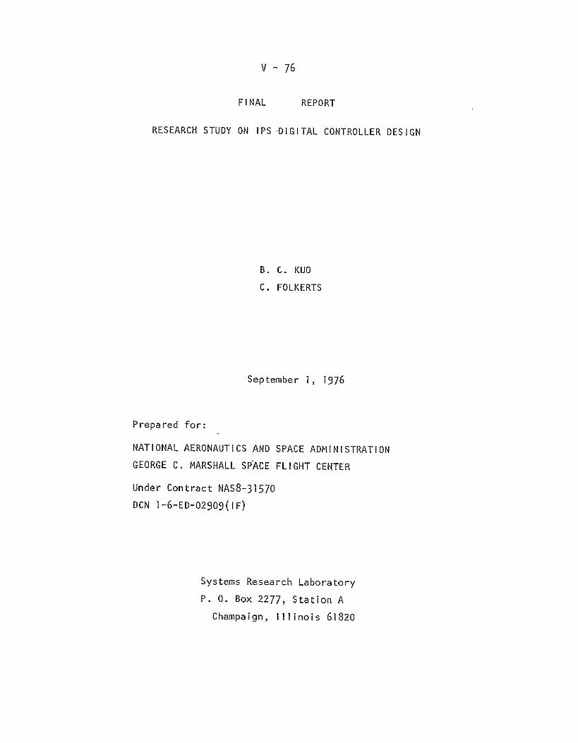
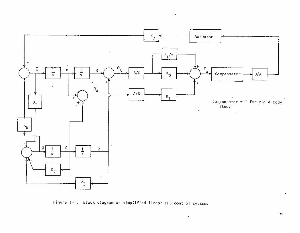
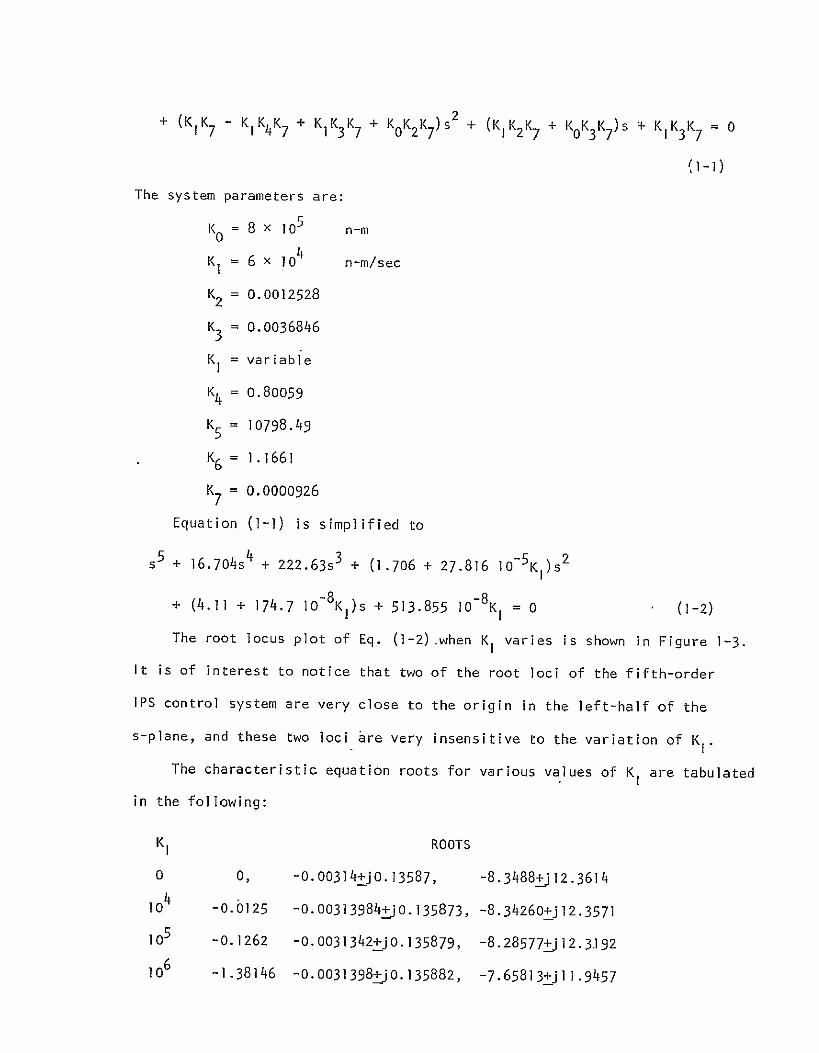

--
SPPP SGIAUARE II)A 010 THEINC AS0801 G0
t __ -- - _ - - shy2 _2 L- _ - X - ----- - -- - shy
- I - -- - -Cg Jflfta ---w-
_ _ _____ -_ __ -__-t-1__ _ _ _ _ _ 4 __ _ _s_ id) _ _ I
------- t
______ - __-l
_____ - - ___-- T-1-2-1
_-i_-_ I _--t__--_--_ I 00 7 - ----
--__I-- L
_ ---- -
- -
-2
- -
- - - --- - --- - -- -I p shy- -- j --_- _-_- -- r--- - - -- -- --- I--- - - -- --
I ___ 1 ForI- Resectcnsiof- LZ tia val fi-et L
--- I _ i - ---- _ _ - --- --z- --- shy
shy-- -__ 1------ - I l - __-_ 1 Irl
-_ - H-
j -t -
_ _ _ _ _ _ _-__-_ i- P -H -tti-4-- -+i-4-j-- -
H-
j
- __ _ _ _
9
period of oscillation The eigenvalues at s = -000313 + jO1358 due to
the isolator dynamics give rise to an oscillation which takes several
minutes to damp out The conditional frequency is 01358 radsec so the
period of oscillation is approximately 46 seconds Figure 1-5 shows the
response of a(t) for a = 1 rad on a different time scale over 100 secondso
Although the initial condition of I radian far exceeds the limitation under
which the linear approximation of the system model is valid however for
linear analysis the response will have exactly the same characteristics
but with proportionally smaller amplitude if the value of a is reduced0
Since the transient response of the system is dominated by the
isolator dynamics with etgenvalues very close to the origin changing
the value of KI within the stability bounds would only affect the time
response for the first second as shown in Figure 1-4 the oscillatory
and slow decay characteristics of the response would not be affected in
any significant way
10
2 The Simplified Linear Digital IPS Control System
In this chapter the model of the simplified digital IPS control
system will be described and the dynamic performance of the system will
be analyzed
The block diagram of the digital IPS is shown in Figure 2-1 where
the element SH represents sample-and-hold The system parameters are
identical to those defined in Chapter 1 An equivalent signal flow graph
of the block diagram in Figure 2-1 is drawn as shown in Figure 2-2
Applying Masons gain formula to Figure 2-2 with A(s) and 0A (s) as
outputs OA(s) and 2A(S) as inputs we have
Gh(s) KIT Gh(s)A) -7 As (A1 - K4)A(S) - (K0 + -- ) - (A1- K )O(s) (2-1)
As4A0 z-1 7 A 1 4 A
Gh(S) KIT Gh(s)CA(S) -KIK 7 As2(A - K4)QA(s) - (K0 + -1)K7 s-(AI K4)0A(S) (2-2)
where A =I+ K s-1 + K s-2 (2-3) 1 2 3 A = 1 - -1 + K3s-2 (2-4)
Gh(s) _I - e (2-5)bull S
Lett ing
Gl(s) = K Gh(s) K7 (1- e-TS)(l - K4)s 2 + K2s + K3) (2-6)1 7 As(A 1 K4) = 2(1_ K4K6 )s 2 + K2s + K3)
G2(s) = K G- (As) K G(s)As2 (2-7)2 s
and taking the z-transform on both sides of Eqs(2-1) and (2-2) we have
K T PA( z ) = -K]G I (z)A(z) - (K0 + Z-1-)G I (zE)A(z) (2-8)
KIT 0A(z) = -KIG 2 (z)amp2A(z) - (K0 + z--G2(Z)oA(z) (2-9)
E A A_
+ +
4 1 Figure 2-1 Block diagram of simplified linear digital IPS control system
2k
-KK K(-
0 A T
Figure 2-2 Signal flow graph of the simplified inear digital IS
control system
13
From these two equations the characteristic equation of the digital system
is found to be
KIT A(z) = 1 + KIGI(z) + (K0 + - G)2(Z) = 0 (2-10)
where2 ( l -7e - i K4
26) s + K 3 1
G2(z) = t(G(s) s ) (2-12)
The characteristic equation of the digital IPS control system is of
the fifth order However the values of the system parameters are such
that two of the characteristic equation roots are very close to the z = I
point in the z-plane These two rootsampare i^nside the unit circle and they
are relatively insensitive to the values of KI and T so long as T is not
very large The sampling period appears in terms such as e0 09 4T which
is approximately one unless T is very large
Since the values of K2 and K3 are relatively small
4K7(l - -1(z) K) ] 7K1- K 6 z4T
= 279x]0-4 T -(2-13)z--)
2G(Z) K 1 K4 (1 - Z1279x1 0- T 2 ( ) 214)1 - K4K6 ) s 3 2(z - 1)
Substituting GI(z) and G2 (z) into Eq (2-10) the characteristic equation
of the digital IPS is approximated by the following third-order equation
z3 3+K0 _PT 2 K K T 33z2 + [KpKT p 3z
KKT 1I p- 2K+ 3 z
3K K1IT K0K Ti2
P2 +K 1 2 (~5
14
where Kp = 279gt0 and it is understood that two other characteristicpI
equation roots are at z = I It can be shown that in the limit as T
approaches zero the three roots of Eq (2-15) approaches to the roots of
the characteristic equation of the continuous-data IPS control system and
the two roots near z = 1 also approach to near s = 0 as shown by the
root locus diagram in Figure 1-3
Substituting the values of the system parameters into Eq (2-15) we
have
A(z) = z3 + (1116T 2 + 1674T - 3)z2 + (3 - 3348T + 1395x10-4KIT3)z
+ (l395xIo-4KIT3 + 1674T - ]l6T 2 - I) = 0 (2-16)
Applying Jurys test on stability to the last equation we have
(1) AI) gt 0 or K K T3 gt 0 (2-17)
Thus KI gt 0 since T gt0
(2) A(-l) lt 0 or -8 + 06696T lt (2-18)
Thus T lt 012 sec (2-19)
(3) Also la 0 1lt a3 or
11395x10-4KIT3 + 1674T - lIl6T - II lt 1 (2-20)
The relation between T and K for the satisfaction of Eq (2-20) is
plotted as shown in Fig 2-3
(4) The last criterion that must be met for stability is
tb01 gt b2 (2-21)
where 2 2b0 =a 0 -a 3
b =a a2 - aIa 3
a0 = 1395xl0- KIT + 1674T - lil6T2 - I
--
to
shy
0 I
lftt
o
[t
-I
-J_
_
CD
C 1_ v
-
1
_
_-
I-
P
I
--
11
-
I i
[
2
o
I
-I
I m
la
o
H-
-I-
^- ---H
O
-I
I
I
-
o
-
--
iI
j I
I
l
ii
-
I
-2 I
1
coigt-
IL
o
Iihi
iiI
I I
-I
--
-__
I
u _
__
H
I
= 3 - 3348T+ 1395x1- 4KIT3
2 a2 = lll6T + 1674T - 3
a = 1
The relation between T and K I for the satisfaction of Eq (2-21) is
plotted as shown in Figure 2-3 It turns out that the inequality condition
of Eq (2-21) is the more stringent one for stability Notice also that
as the sampling period T approaches zero the maximum value of K I for
stability is slightly over I07 as indicated by the root locus plot of
the continuous-data IPS
For quick reference the maximum values of K for stability corresshy
ponding to various T are tabulated as follows
T Max KI
71O001
75xo6008
69xio 6 01
When T = 005-sec the characteristic equation is factored as
(z - l)(z 2 - 0884z + 0442 - O1744x10-7K ) = 0 (2-22)
Thus there is always a root at a = I for all values of KI and
the system is not asymptotically stable
The root locus plot for T = 001 008 and 01 second when KI
varies are shown in Figures 2-4 2-5 and 2-6 respectively The two
roots which are near z = 1 and are not sensitive to the values of T and
KI are also included in these plots The root locations on the root loci
are tabulated as follows
17
T = 001 sec
KI
0 100000
106 09864
5x10 6 0907357
107 0853393
5x]07 0734201
108 0672306
T = 008
KI
0 0999972
106 0888688
5XI06 00273573
6 75xi06 -0156092
107 -0253228
108 -0770222
ROOTS
091072 + jO119788
0917509 + jO115822
0957041 + jO114946
0984024 + jO137023
104362 + jO224901
107457 + jO282100
ROOTS
-00267061 + jo611798
00289362 + jO583743
0459601 + jO665086
0551326 + j0851724
0599894 + j0989842
0858391 + j283716
NO341-
D
IE T
ZG
EN
G
RA
P-H
P
AP
E R
E
UG
E N
E
DIE
TG
EN
tCOI
10
X
O
PE
INC
A
IN U
S
ll ll
lfti
ll~
l~
l l Il
q
I i
1 1
i I
i
1
1
i
c
I-
I
I-I
I
f i l
-I-
--
HIP
1 I
if
~~~~
~1
] i t I
shyjig
F
I i
f i_~~~~i
I f 1
I
III
Il
_
i
f I shy
1
--I - shy
n
4 q
-- -shy-
-
4-
----L-
- -
TH
-shy
r
L
4
-tt
1--
i
-
_
-shy
_
-----
_
_ _ L
f
4 ---
----
-shy--shy
~
~ i
it-i_
-_
I
[ i
i _ _
-shy
m
x IN
CH
A
SDsa
-c]
tii
-
A
I-A-
o
CO
-
A
A
A
-A
A
N
I-
A
-
-
IDI
in--_ -
--
r(
00A
7 40
I
CD
-I
ED
Ii t4
]
A
0 CIA
0w
-tn -I
S
A- 0f
n
(I
__
(C
m
r S
QU
AR
ETIx
110T
OE
ICH
AS0
807-0)
(
-t-shy
7
71
TH
i
F
]-_j
-
r
Lrtplusmn
4
w
I-t shy
plusmn_-
4
iI-
i q
s
TF
-
--]-
---
-L
j I
-- I
I -
I -t
+
-
~~~4
i-_
1 -
-
-
-
---
----
-
-
I_
_
_ -
_ _I
_
j _
i i
--
_
tI
--
tiS
i
___
N
__
_ _
_ _
_
-
-
t --
-
_ _I__
_
_
__
-
f
-
J r
-shy
_-
-
j
I
-
L
~
~ 1-
i I
__
I
x times
_
_
i
--
--
-
--
----
----
----
---
---
-
i
-
I
o-
-
i
-
-
----
-
--
I
17
-_
x-
__
_-
-i-
-
i
I__
_ 4
j lt
~
-
xt
_ -_
-w
----K
-
-
~~~~
~~~~
~~~~
~~
-
-
l]
1
i
--
-
7
_
J
_
_
_
-
-_z
---
-
i-
--
4--
t
_
_____
___
-i
--
-4
_
17 I
21
T =01
K ROOTS
0 0990937 -0390469 + jO522871
106 0860648 -0325324 + j0495624
5xlO 6 -0417697 0313849 + jO716370
7xlO6 -0526164 0368082 + jO938274
07 -0613794 0411897 + jl17600
108 -0922282 0566141 + j378494
The linear digital IPS control system shown by the block diagram of
Figure 2-1 with the system parameters specified in Chapter 1 was
simulated on a digital computer The time response of e(t) when theshy
initial value of c(t) c6 is one isobtained Figure 2-7 illustrates
the responses of c(t) for T = 001 KI = 5xO 6 and T = 01 KI = 105
and KI = 106 Similar to the continuous-data IPS control system analyzed
in Chapter 1 the time response of the digital IPS is controlled by the
closed-loop poles which are very near the z = I point in the z-plane
Therefore when the sampling period T and the value of KI change within
the stable limits the system response will again be characterized by
the long time in reaching zero as time approaches infinity
The results show that as far at the linear simplified model is
concerned the sampling period can be as large as 01 second and the
digital IPS system is still stable for KI less than 107
COUPC~PCP1ION SuIF~~oN~wyoSQUARE IS x I 10TOM ICH AS -GO~~(~)
2
~I------
-~~_~l~
1 shyW-
-I 4
-_ _ --_I- -
1I
F~- -
_
__--shy___shy
_
2 _ -
_-71__
shy 4-f e do
F I f
i- iL _I
_ - r--ny n--4 F7 I7kp-- - _-- -4-- - 4- _ --- - ---
-
K -
-
5 -it 0 -shy
~ _-
t I i- (Seconds -shy 4-IL4
-- - -
-
E -
- - 4 -
_ -
_- _
_ -shy
-- _ __ __-_ __ _ -L_ -____ -ILE H 5-4-_-_-----_-_
_
_ _
-
j2ZI-4-
-
- -I
I r
9
- --
1
-
23
3 Analysis of Continuous-Data IPS Control System With Wire Cable
Torque Nonlinearity
In this chapter we will conduct a stability analysis of the simplified
IPS control system with the nonlinear characteristics of the torques caused
by the combined effect of the flex pivot of the gimbal and by wire cables
for transmitting power etc across the gimbal to the experiment as shown
in Figure 3-1
The flex pivot torque disturbance has been modeled2 as a linear spring
with slope KFP as shown in Figure 3-2 The wire torque disturbance is
modeled as a nonlinear spring with a slope of KWT as shown in Figure 3-3
The total torque disturbance associated with the flex pivot and wire cables
is summed up as shown in Figure 3-4 The continuous-data IPS control system
with the nonlinear torque characteristics is shown in Figure 3-5
The objective of the analysis in this chapter is to study the condition
of sustained oscillation of the nonlinear IPS control system shown in
Figure 3-5
The Describing Function of the Wire-Cable Nonlinearity
It was pointed out in the above discussion that the wire cable
nonlinearity can be modeled by either the arrangement shown in Figure 3-4(a)
or Figure 3-4(b) For the model of Figure 3-4(a) a relay characteristic
is present between a and Tc and in addition a linear gain of KWT + KFP
exists between E and TC where KFPdenotes the gain constant due to the flex
pivot torque Using this model one can conduct a describing function
analysis with the relay nonlinearity but the linear system model is altered
by the addition of the branch with the gain of KWT + KFP However careful
examination of the block diagram of Figure 3-5 reveals that the branch with
Figure 3-1 Experiment with wire cables
25
Torque (N-m)
K (N-mrad)FP
------ c (rad)0
Figure 3-2 Flex-pivot torque characteristic
Tor ue (N-m) I HWT (N-m)
Z ~~ c (rad)
KW (N-(rad)_
Figure 3-3 Wire cable torque characteric
26
T KF
poundWHWT ~HWT + C
(a)
T
K(FP+KwHW
(b)
Figure 3-4 Combined flex pivot and wire cables torque
characteristics
WTI)
DO 1 p
rigure 3-5 PS control system with the
nonlinear flex pivot and wire cable torque
Kcs character ist
28
the gain of KWT + K is parallel to the branch with the gain KO which has
a magnitude of 8x)0 5 N-mrad Since the value of KWT lies between 025 and 25 N-mrad and the maximum value of K is in the order of several hundred
it is apparent that the value of K0 will be predominant on Lhe system
performance This means that the linear transfer functionwillnot change
appreciably by the variation of the values of KWT and KFP
Prediction of Self-Sustained Oscillations With the Describing
Function Method
From Figure 3-5 the equivalent characteristic equation of the nonlinear
system is written as
I + N(s)G eq(s) = 0 (3-1)
where N(s) is the describing function of the relay characteristic shown in
Figure 3-4(a) and is given by
N(s) = 4HWTr5 (3-2)
The transfer function Geq(s) is derived from Figure 3-5
G eq
(s) - 00013946(s 4 + 00012528s 3 + 00036846s2) (3-3)A(s)
where A(s) = 5s + 16704s4 + 2226s 3 + (2781xlo4K 1+1706)s 2
+ (411 + 1747xO-6KI)s + 513855xO-8 Ki1(3-4)
A necessary condition of self-sustained oscillation is
Geq(s) = -1N(s) (3-5)
Figure 3-6 shows the frequency response plots of Geq (s)for K = 105 106 and 107 a function of and the trajectory of -1N(s) =- 4HWT
as w
NO 34- aDICTZGEN ORAPH PAPER EUGENE DIETZOEN CO MA E IN U S A
1O X I PER INCH
OF TRF-ttOBiI+t_
I f i l l -I __ re
h shy-HIE hh 4 i zj-+ shy4-
I- 4+ -H I 1
I t j-I
-L)
------ gt 4~~ jtIi 11 --- - -41 -a Itt- i
i i li L 2 4 I __-- __-_
_ _++_A _ I iI I It I T-7 1
- _ i h-VK0 L qzH1 -LiT ____-___-_-
~ ~ - OrtIldf~jj plusmnL -e ~ ~ ~ fl pdffle
I-I____+1 [+ Flr___ fI
30
the latter lies on the -180 axis for all combinations of magnitudes of C and
HWT Figure 3-6 shows that for each value of KI there are two equilibrium
points one stable and the other unstable For instance for KI = 10- the
degGeq(s) curve intersects the-180 axis at w = 016 radsec and w = 005 radsec
The equilibrium point that corresponds to w = 016 radsec is a stable equilishy
brium point whereas w = 005 radsec represents an unstable equilibrium point
The stable solutions of the sustained oscillations for K = 105 10 and l0
are tabulated below
KW HWT (radsec 6HwT (rad) (arc-sec) (radsec) c (sec)
107 72x]o-8 239xI0 -7 005 03 21
106 507x]0-7 317x10 6 39065 016-
105 l3xlO-5 8l9xlo - 5 169 014 45
The conclusion is that self-sustained-oscillations may exist in the
nonlinear continuous-data control system
Since the value of K 1-svery large the effect of using various values 0
of KWT and KFP within their normal ranges would not be noticeable Changing
the yalue of HWT has a one-to-one effect-on the amplitudes of oscillations
of E and C
Digital Computer Simulation of the Continuous-Data Nonlinear IPS Control System
Since the transient time duration of the IPS control system is exceedingly
long it is extremely time consuming and expensive to verify the self-sustained
oscillation by digital computer simulation Several digital computer simulation
runs indicated that the transient response of the IPS system does not die out
after many minutes of real time simulation It should be pointed out that the
31
describing function solution simply gives a sufficient condition for selfshy
sustained oscillations to occur The solutions imply that there is a certain
set of initial conditions which will induce the indicated self-sustained
oscillations However in general it may be impractical to look for this
set of initial conditions especially if the set is very small It is entirely
possible that a large number of simulation runs will result in a totally
stable situations
Figure 3-7 illustrates a section of the time response of e(t) from t = 612
sec to 692 sec The initial conditions are c(O) = 10 and E(0) = 10 and
allother initial conditions are set to zero KI = 105 HWT = 1 and KWT + KFP
= 100 It was mentioned earlier that the system is not sensitive to the values
of KWT and KFp From Figure 3-7 it is seen that the period of the oscillation
is 48 seconds or 013 radsec which is very close to the predicted value
0
Time (sec) c(t)
61200E 02 -47627E-05 -+
61400E 12 -265 E-05 ------------------------shy6 16iOE 02 -23637E-06 --------------------------shy618 00E 02 1 6859E-C5 ---------------------------- + 62I0E 02 231E-5 - ----------------------------b22~0HE 02 38527E-05-------------------------------shy6 2400E 02 49397E-05- ------------------------------E26 0OE 0 6 1609E-05 ------------------------------ +
SOCE 02 70494E-05 ------------------------------ + F JCE 02 5BO E 0 610C0E 02 6333E-05--------------------------------shy
-64320 02 5036E-05--------------------------------shy6 3400E 02 41 3i9E-05 --------------------------63600E 0 26582_E-----------------------------shyt( 80E 02 2 078E-05 ----------------------------64000E 02 -4 5 E-06 -------------------------shy
64200E 02 2042E-05 -------------------------- + 644 0OE 02 -346 1E-05 -------------------------64600E 02 - 1003E-05- -----------------------shy
r 400E 02 -61067E-05 ------------------------D 500E 02 -6 1478E-05 ----------------------- +
- 6520]0E 02 -5 6092E-05 ------------------------65400E 02 -51468E-0 ------------------------shy
o 65600E 02 -5 SE- ------------------------shy6 58OCE 02 -42871E-05 ------------------------66000E 02 -29645E-05 ------------------------- +
06200E 02-- -9329 0E- 0-shy-t 16400E 02 1 2747E-05 --------------------------- +
6S6400E 02 1 824E-05--------------------------------668-O0E 02 31904E-05 ---------------------------shy
67000CE 02 419042-05- -------------------------------- + 6720]0E 02 41_SE-05 ----------------------------- + 67400E 02 4 583E-05- ------------------------------
CD 760uE 02 i E- ------------------------------shy
6b78b0E 02 56122OE-05---------------------------------62000E 02 461205E-05_ ----------------------------- + 6 2 02 ---------------------------U00E 24641E- 05
65400E 02 99768E-06 --------------------------- + 6_260OE 02 54662- 0-_E --------------------------- + 68H00E 02 -87772E-06 -------------------------shy6 U00E 02 -2145E-05 ------------------------ + 69200E 02 -- 5 751E-05 ------------------------shy
33
4 Analysis of the Digital IPS Control System With Wire Cable Torque -
Nonlinearity
In this chapter we will conduct a stability analysis of the simplified
digital IPS control system with nonlinear characteristics of the torques
caused by the combined effect of the flex pivot of the gimbal and wire cables
The analysis used here is the discrete describing function which will
give sufficient conditions on self-sustained oscillations in nonlineardigital
systems The block diagram of the nonlinear digital IPS system is shown in
Figure 4-1 For mathematical convenience a sample-and-hold is inserted at
the input of the nonlinear element
A signal flow graph of the system in Figure 4-1 is drawn in Figure 4-2
The z-transforms of the variables in Figure 4-2 are written
SA (z) = -G2 (z)Tc(z) (4-1)
QA(z) = -Gl(z)Tc(z) (4-2)
H(z) = G4 (z) Tc (z) (4-3) KIT
Tc(Z) K QA(z) + (K + T) OA(Z)
-(KWT + KFP )G3 (Z)Tc (z) + N(z) (z) (4-4)
where G0(5) shy
01(z) = h (A 1 - K4)J
(z) =ZKGCA KK7
K Gh(s)3 (z) 7
3= =
7 As lJI G4(z) Gh(s) AdlK7 hAS
s-e-Ts Gh (s)
A2 = I + K2s-I + K3s-2
++
KO+--
H
S S
the nonlinear flex pivot and wire cable torqueEl characterist ics
U)
AT T
-4K 6zG 2
logg
T T K T
i
36
A = ( - K4K6) +-K2s- + K3s-2
N(z) = discrete describing function of ideal relay (+HwT 0 -HWT)
Since K2 and K3 are very small approximations lead to
G0(z) = 279 10-4T z 2- +
1)G2 (z) 279 1-4T2(z + 2(z - 1)2
0000697T1(z + 1)
3z 2(z - I)2
00001394TG4(z ) z - 1
Equations (4-I) through (4-4) lead to the sampled flow graph of Figure
4-3 from which we have the characteristic equation
A(z) = I + KiG (z)+ K + _1- G2 (z)+ (KwT + KFp)G (z)+ G4 (z)N(z) (4-5)
Equating A(z) to zero the equivalent transfer fucntion G (z) is obtainedeq G4(z)
Geq(z) = - KIT (4-6)e + KiG (z) + Kdeg + Z jG2 (z) + (KwT + KP) 3(z)
The intersect between G (z) and -IN(z) gives the condition of selfshyeq
sustained oscillations in the digital IPS control system
Figure 4-4 shows the Geq (z) plots for various values of Ngt-2 for KI = 105
In this case it has been assumed that the periods of oscillations are integral
multiples of the sampling period T Therefore if T denotes the period of
oscillation Tc = NT where N is a positive integer gt 2
From Figure 4-4 it is seen that when N is very large and T is very small
Geq(z) approaches Geq(s) However for relatively large sampling periods
37
-G2(z)
-G (z N(Z)
-
Figure 4-3 Sampled signal flow graph of the digital IPS
control system
Geq (z) does not approach to G (s) even for very large N This indicates
the fact that digital simulation of the continuous-data IPS can only be
carried out accurately by using extremely-small sampling periods
The critical regions for -IN(z) of an ideal relay are a family of
cylinders in the gain-phase coordinates as shown in Figure 4-5 These
regions extend from --db to +- db since the dead zone of the ideal relay
is zero For N = 2 the critical region is a straight line which lies on
the -180 axis The widest region is for N = 4 which extends from -2250
to -135 Therefore any portions of the G (z) loci which do not lie ineq
the critical regions will correspond to stable operations
It is interesting to note from Figure 4-4 that the digital IPS system
has the tendency to oscillate at very low and very high sampling periods
but there is a range of sampling periods for which self-sustained
oscillations can be completely avoided
l- Zit iii n 1 i - iyo t-- _ __-_ I -
-
--- o it Th t r-tshy
--shy
4
+ - - - o5 s -
- - _- - - - - -- - - I I
-- A T-- ----- o o
-
N-4ltshy
_
--shy
-(_) shy
61 -Idao
-
I
-_ I --
rZ
]- - r-u cy-response plt-----
jFigure i-4en___
a G-4 forvar ioi Isva]Ues of -
-shy ---shy [- _ _ - b - = 7
- -- -- --
-- __-____ ~4 -- t-~ -- - i r -
r
_
--
- -
-
o-
-- -shy
tj______
ID
-
-
__ ______
I
deg--
_-
_ _
_ shy
_--
_ _
-- -- I-- shy- f ttr-Z -- 300 I -260o-2T - 0- - - 10 = 10 -1 o - -o- -6 - - -r- r H f I1 I -- 1 --- f- - DE R Es r_--- -l -- -- - ~-- - ~-- - -v- - 4 t - I 1 0
AlA tr
1 ~ ~
In
L w I-m1th7 - I--r-I-
~ ~ 7 1 1--r1~
I
-shy 7
1- 0 c17
_ _
A
r qIo
___
Ia L
I Ill ~ - ---- --
II7 -LI 4 --- - I 1
[-- - r- lzIjIiz --i-i--- [ ii - - -L _
- - i - --
[J2jV L L f
I
-__
- _ _- - -
Te
- -
ayshy
-__
deL-Lr-i-b
l _ _ I-shy
________ ~ H- t1 sectj4--ffff
e
-i-i-desc
____shy i
I~At ~~~~-7= AITtt-
~ T_
_ S
1 ___ _IAI
5A
_
IP
-
4
_____ __ __
_
~
__
_
__
___t-j --
___ __ ____
L
Referring to Figure 4-4 it is noticed that when the sampling period T
10~2 is very small (T lt sec approximately) the loci of Geq(z) for N = 2
3 and 4 lie in their respective critical regions and self-sustained
oscillations characterized by these modes are possible However since the
actual period of these oscillations are so small being 2 3 or 4 times
the sampling period which is itself less than 001 sec the steady-state
oscillations are practically impossible to observe on a digital computer
simulation unless the print-out interval is made very small This may
explain why itwas difficult to pick up a self-sustained oscillation in the
digital computer simulation of the continuous-data IPS system since a
digital computer simulation is essentially a sampled-data analysis
When the sampling period is large (T gt 9 sec approximately) the digital
IPS system may again exhibit self-sustained oscillations as shown by the
Geq(z) loci converging toward the -1800 axis as T increases However the
Geq(z) loci of Figure 4-4 show that there is a midrange of T for which the
digital system is stable The Geq(z) locus for N = 2000 actually represents
the locus for all large N Therefore for T = 01 the Geq(z) locus point
will be outside of the critical regions since as N increases the widths
of the critical regions decrease according to
N = even width of critical region = 2urN
N = odd width of critical region + 7TN
Therefore from the standpoint of avoiding self-sustained oscillations
in the simplified digital IPS control system model the sampling period may
be chosen to lie approximately in the range of 001 to I second
41
Digital Computer Simulation of the Digital Nonlinear IPS
Control System
The digital IPS control system with wire-cable nonlineari-ty as shown
by the block diagram of Figure 4-1 has similar characteristics as the
continuous-data system especially when the sampling period is small The
digital IPS control system of Fig 4-1 without the sample-and-hold in front
of the nonlinear element was simulated on the IBM 36075 digital computer
With initial conditions set for c and S typical responses showed that the
nonlinear digital IPS system exhibited a long oscillatory transient period
Figure 4-6 shows the beginning portion of the response of 5(t) for s(O) = 10- 3
-4(0) = 10 K I = 105 T = 01 sec HWT = 1 KWT + KFP = 100 Figure 4-7
shows the same response over the period of 765 sec to 1015 seconds Figure
4-8 gives the response of E(t) for the time duration of 1530 sec to 1725 sec
and it shows that the response eventually settles to nonoscillatory and
finally should be stable
---------------------------
Time (sec) e(t)
0 0 1 9000 E-04 ----------------------------- ----shy
487-0450 ]E2 400- - -10I0E 01 -- - 2E 0E- shy0 +E--4
- 15000CE 01 -1 6-E- 5 shy I E ll 2311 8E-4------------------------------------------
C 25000E 01I 4 2-1)i4S -01 101 i 4 032E-04-------------------------------------------------------shy- 50lOE 01 4334E-04 ------------------------------------------- + I 40 0 -44-2E-04 +------------------------------------shy
45000245000 E --46699-054 -----------shy0101 3095 3E -04 -------------7 ---shy
(D 5000E 01 -43414E-04- -------------shyi (a 55000E 01 -amp6717E-04 ---------------shy0 - 60000E 01 -14427E-04--------------------------shy
9i65000 E 01 1843E-04 --------------------------------------shy-- 70000 01 E-04--- -----------------------------------------------shy
0 7500 CE 01 4036E- 1-----------------------------------------------shy01 29-04-_000CE ------------------------------------------- +
8~ 36615E-05------------------------------------shy5000E 01 09000011 01 -22174E-04--------------------------Oh 5IE 01 -37802E-04-----------------shy
1 0000E 02 -3492-04 ----------------shy-1 95002 02 -1 33E-04-----------------------------11000E 02 __-63194E-05-- -------------------------11500E 02 173434E-4 --------------------------------------shy1200E 02 2264 -04----------------------------------shy
o 12500E 02 1 EZi4 +-shy
- 1 3000E 02 47188E-05 ---------------------------------13500E 02 -71956E-0a--------------------------------+
1L14000E-0---1---4E04--------------------7-------shyI1 4500E 02 -1 74_E-0--4 ------------------------
100E 02 -1 - 0-04- ---------------------------1550OE 02 -149E 4--------------------------------shy4
16 0E 02 - 1-344E-04 ----------------------------------- shy
o) E 169 u E 02 18073E-04------------------------------------------shy1700ii0E 02 1 6576E- 04------------------------------------------17500E 02 77892E-05--------------------------------------shy1 8000E 02 -2 2145E-05----------------------------------shy1 8500E 0 -1 14--------------------------19000E 02 -1 644E-04 ------------------------- + 1 950E 02 -1 1929E-04 + 200LE 02 -27840 E-- ------------------------------shy21 _E 02 1 47-E- 054-----------------------------------
21000E 02 15121E-04- ------------------------------------shy
Time (sec) s(t)
7 6500E 02 42449E-05 --------- +
7 7000E 02 46277E---5 -- --------------------------------- + 77500E 02 2 5093E-05 -------------------------- --- + - 78000]E OS- -371--E-06 -+
OjII 2 --- --7 M E I]2- -2 S n --- -- -- --- ----- =S7 nnnE -- ---i02 -- shy Io IJ-E-
S500E 02 -2 9759E-i-05 -shy
iA 00E 02 -6 2_116E-06 --shy
S1500E 02 -2 1103E-05 ------------------------ --- -+8 O1E 2 -- 21 E -- --
81500E 02 2279E-05 -- - + - 1000-E 02 48384E-0 -- ------------------------- - +
On0 153002E S 8500E 02 -23254E-05 +---------------------shyo _8 _5 IOTa- 42021E-0E-06F - --------------- --- -- -shy II0E 02 37490i -- -- - ---- ---
00E 2 -8 -711E-05 - -
M-- -- - -- - shy+ 045E 02 -101671E-05 ------------------------------------- +
4005I00E 0202 31- 05- -------------------------------- +S5000 3 E- 0 -----------------------------------
86000E 02 8522E--05 ---------------------------------86500E 02 29366E-05----- ---------------------------
SAME 93945E-lI6 -----------------------------------shy2
87500E 02 -1 2310-0 -------------------------------E-800E0 - 2GA v------------------------------- +
0- 0E QOE 02 -1 1E- -----------------------------shy
oj 89500E 02 69699E-0 ------------------------------- +
8 8 -026411E- 05 - shy
90 00 02 2537-0-------------------------------shyo 9 0500E 02 3 19E-= --------------------------------
91000E 02 28 5E-05 -------------------------------- +
3 9 1500E 02 1 3396E-0---------------------------- 7------- c-
- 2000E 02 -441E-- ------------------------------shy92500E 02 0-20198E--5 ------------------------------ + 93 00E 02 -23537E-05 ----------------- ------------- +
- 9300E 2 -1 4725E-05 ------------------------------ +
ii 9 4000E 02 2 -E-0 -------------------------------shyo 94500q20200 1 E-----------------------------------Z 95000E 02 9036E-05 -------------------------------- +
95500E 02 2T71E-05- -----------------------------shy + 02E02 16172E-05 -------------------------------- +
_ -39172E-07 --------------------9650OE 02 -71OIE-02 -1 4506E-05 ------ ----------------- -------- + 97500E 02 -2 0075E-05 ------------------------------ + I O00E 02 -14941E-05 -----------------------------shy
500E 02 -1 6809E-o_ ------------------------------- + 9 OE 02 1 3r672E-05 ------------ ------------------- + 99500E 02 2429-0--5 -------------------------------- +
1 000E 03 25769E-05 -------------------------------- + 1 0050E 03 1 654E-05 --------------------------------I1OiOOE 03 1 ------------------------------shy3 6 0 101502 3 -94976E-06 ------------------------------- +
--------------------------------------------------------------
--------------------------------------------------------------
--------------------------------------------------------------
-----------------------------------
-n
O
o shyo 0 I (
(D oo -h
= 2
0o
II m
C 0
+1 01 2 + shy
0
Time (sec)
15302 0315350E 03
15400E 03 1 5450E 13
E(t)
-3 0269E-07 6569-
12387E-06 59750E-06
0315500E77)6E-06 1 5550E 007 1 5600E 03 1 5650E2 03 1570 0E 0 15750E 03
1 5850 E 03 1 5900E 03 1 5950E 03 1S00E 03
16050E 03 1 6100E 03 16150 03 16200E 03 1 250E 03 16300E 03 1 6350E 03 1 402 03 1 6450E 03 1 6500E 03 1w6550E 03 1 660E 03
6650 2 03
6700E 03-16750E 03 169502E 03 1 - 0E 0 16900UE 03-
17100E 0317050E OS
17100E 03
1 7150E 03 1 7200E 03 172502 03
681E-06
--- -shy
-- - - - -- - - - - -- - - shy --+
-+ - +
62441E-06- ------------------------------shy36730E-06---------------------------------shy1 3305E-06 26 2E-07-
28820E-0 5297- 06 70821E-06 74646E-06 631902-06 42071E-2 0731E-06 84777E-1 0379E-06 2530 0- shy46163E-06
-- ---shy------------------------------shy------------------------------shy------------------------shy------------------------------shy
+ + +
------------------------------shy------------------------------shy
63 ---------------------------------shy70292E-06 ------------------------------- +
63401E-06---------------------------------shy46612E-06-------------------------- -------- + 275 9-06 -------------------------------shy1 4624E-06 ------------------------------shy1 31E-06 -------------------------------shy
-552E-06- ------------------------------shy05-
57316E- O------------------------------shy65755E-06 +
490E-06- ------------------------------shy2889E-0 -- -- -- - -- -- -- - -- -- shy
I90 EE-06 -- - - - - - - - - - - - - - shy
16209E-06 ------------------------------shy2 33 E- - -------------------------------shy37732E76I---------------------------shy
45
5 Gross Quantization Error Study of the Digital IPS Control System
This chapter is devoted to the study of the effect of gross quantization
in the linear digital IPS control system The nonlinear characteristics of
the torques caused by the combined effect of the flex pivot of the gimbal
and wire cables are neglected
Since the quantization error has a maximum bound of +h12 with h as the
quantization level the worst error due to quantization in a digital system
can be studied by replacing the quantizers in the system by an external noise
source with a signal magnitude of +h2
Figure 5-1 shows the simplified digital IPS control system with the
quantizers shown to be associated with the sample-and-hold operations The
quantizers in the displacement A rate QA and torque Tc channels are denoted
by Q0 QI and QT respectively The quantization levels are represented by
ho h and hT respectively
Figure 5-2 shows the signal flow graph of the digital IPS system with
the quantizers represented as operators on digital signals Treating the
quantizers as noise sources with constant amplitudes of +ho2 +hi2 and
+hT2 we can predict the maximum errors in the system due to the effect
of quantization The following equations are written from Figure 5-2 Since
the noise signals are constants the z-transform relations include the factor
z(z- )
T KoK++z) h 1 (KT -Kz 7Gh(S)l( ) 4 h(S)K h z
2A(z) 7hsI + 47h I_ ()+LI- (5-2) 0 2 z1(-1
OA(Z)~ -7hSA(s2 7h()s - 2 z A(s) 2s)
K 4SHQlK I shy
0 Sshy
2 ~~~Figure 5-1 Linear simplfe iia P control syse wihun za o
-K 6 K
s Kdeg
-~ ~~~f- T OAq zT
KK
K-2 Fiur S6na sipiTe dTgISsse wt un~ Tloin Trp Tof
48
The last two equations are written as
hT 0A(z) = G(z) T (z) + 27 (5-4)
eA(z) = G2 (z)T (z) h (5-5)
-2 where AI(s) = I + K2s- + K2s (5-6)
A(s) = 1 - K4K 6 + K2s-I + K3s-2 (5-7)
G1 (z) 2782z1x]O-4T (5-8)- T
1 ~z -I
G2(z ) = 2780-4T2(z + )(5-9)2(z - 1)2
Figure 5-3 gives the digital signal flow graph representation of Eqs (5-i)
(5-4) and (5-5) Using Figure 5-3 we can analyze the worst-case errors due to
quantization in the steady state at any point of the IPS system
As derived in previous chapters the transfer functions GI (z) and G2(z)
are given in Eqs (5-8) and (5-9) The characteristic equation of the system
is obtained from Figure 5-3
K T A(z) = I + K1G(z) + K + G2 (z) (5-10)
We shall now evaluate the maximum steady-state quantization errors for 0A 0A and Tc in terms of the quantization levels ho h and h
From Figure 5-3 To(z) is written
f hf+ ] T hTTc(Z) = 1 - --a( I KIT~+ Lh K T] ___K + GKN + ]2(z)]z (5-11)= AtI 2 + z -ldt- 2 I1 +fLK + z-1J1 2 z - I (-i
The steady-state value of Tc(kT) is given by the final-value theorem
lim Tc(kT) = lim (0 - z-I)Tc(z) (5-12) ku o z-1
Substitution of Eq (5-Il) into Eq (5-12) we have
49
h (5-13)lim T (kT) = +- ( - 3k _gtoc 2
S imi larly
-ho KIT] +h hT
+ K1 41G(z)OA(Z) = +K + K- 1) - G2 z(5-14)
Then shyim OA(kT) = im (1 - z-1)e (z)= h (5-15) kzrl A 2
1 ho K T ] hl hiZ aA(Z) = y-K + T- I K1 T G(z) z (5-16)
Iim 2A(kT) = im (0 - zl )QA(z) = (5-17)
Therefore we conclude that the maximum error in Tc due to quantization
is + hT2 and is not affected by the other two quantizers The quantizer in
the eA channel affects only 0A(z) in a one-to-one relation The quantizer
in the PA path does not affect either 0A QA or Tc
-G2(z)
-G (z)
2 z z-
K T I shy
0 z-I
+T z 2 z-l+ ho
2 z- I
Figure 5-3 Digital signal flow graph of the simplified digital IPS with quantization
50
6 Describing Function Analysis of the Quantization Effects-of the Digital
IPS Control System
In this section the effects of quantization in the digital IPS control
system are investigated with respect to self-sustained oscillations
Since the quantizers represent nonlinear characteristics it is natural
to expect that the level of quantization together with the selection of the
sampling period may cause the system to enter into undesirable self-sustained
oscillations
The digital IPS control system with quantizers located in the 0A 2 A and
T channels is shown in Figure 5-1 We shall consider the effects of only one
quantizer at a time since the discrete describing function method is used
With reference to the signal flow graph of Figure 5-2 which contains all
the quantizers-we can find the equivalent character-stic equation of the
system when each quantizer is operating alone Then the equivalent linear
transfer function that each quantizer sees is derived for use in the discrete
describing function analysis
Quantizer in the eA Channel
Let the quantizer in the SA channel be denoted by Q0 as shown in Figure
5-2 and neglect the effects of the other quantizers Let the discrete
describing function of Q be denoted by Q (z) From Figure 5-2 the following
equations are written
Tc(Z)= K0 + I IT Qo (z)A(z) + K12A(z) (6-1)
z-K7 Gh(S) A (s) K4K 7 Gh (s)] E)A(Z) = - 2 A+ 2A Tc(z)
=-G 2(Z)Tc(z) (6-2)
51
A-K7Gh(S)A (s) K4K 7Gh(s) zA (Z) = --h+)I- Tc(Z)
= -GI (z)Tc(Z) (6-3)
where AI(s) = I + K2 s-I + K3s- 2 (6-4)
A(s) I - + K2s - I + K3 s-2K4K6 (6-5)
278x10-4TG(Z) shy (6-6)
G2(z) - 278xO-4T2 (z + ) (6-7)) 2
2(z-
A digital signal flow graph portraying-Eqs (6-1) (6-2) and (6-3) is
shown in Figure 6-1 The characteristic equation of the system is written
directly from Figure 6-1
Qo ( z )A(z) = I + G2(z) Ko + -z- I + K1GI(z) = 0 (6-8)
To obtain the equivalent transfer function that Qo(Z) sees we divide both
sides of Eq (6-8) by the terms that do not contain Qo(z) We have S KIT
Q-f=G (z) K +
1 + 1+ K 1 ( JG qo(z) = O (6-9)KIT
Thus G2(z) Ko + z - (6-1)
eqo KIG1(Z)+ 1
Quantizer inthe A Channel
Using the same method as described in the last section let Ql(z) denote
the discrete describing function of the quantizer QI When only QI is
considered effective the following equations are written directly from Figure
5-2 OA(z) = -G2 (z)T (z)c (6-11)
QA(Z) = -G(z)T (z) (6-12)
TC (Z) = K + Z QA(z) + K1Ql(z) A(Z) (6-13)
52
Q-(z)K o + KIT
ZT(z)
Figure 6-1 Digital signal flow graph of IPS when Q is in effect
KIT
A z- 1
KIQ+( )T-Z
oA
-G2(Z)
Figure 6-2 Digital signal flow graph of IPS with QI if effect
53
The digital signal flow graph for these equations is drawn as shown in
Figure 6-2 The characteristic equation of the system is
A(z) = I + K1GJ(Z)Q(z) + G2 (z) K0 + zK-T01 = o (6-14)
Thus the linear transfer function Q(z) sees is
KIG (z)
Gl z ) (z)1 + G 2(z) (Kdeg -T (6-15)Gq 0 + K T 3
Quantizer in the T Channel
If QT is the only quantizer in effect the following equations are
wtitten from Figure 5-2
eA (z) = -G2 (z)QT(z)Tc(z) (6-16)
QA (z) = -GI (z)QT(z)Tc (z) (6-17)
Tc(Z) = K + KIIA(z) + KlA(z) (6-1-8)
The digital signal flow graph for these equations is drawn in Figure 6-3
The characteristic equation of the system is
K T A(z) = I + KIGI(z)QT(z) + 02 (Z)QT(Z) K + I 1 0 (6-19)
The linear transfer function seen by QT(Z) is
GeqT(Z) = KIG I(z) + G2 (z) [K + (6-20)
The discrete describing function of quantizershas been derived in a
previous report3 By investigating the trajectories of the linear equivalent
transfer function of Eqs (6-10) (6-15) and (6-20) against the critical
regions of the discrete describing function of the quantizer the possibility
of self-sustained oscillations due to quantization in the digital IPS system
may be determined
54
KIT
0 z-l
-GI~)Tc(z)
Figure 6-3 Digital signal flow graph of IPS with IT in effect
Let Tc denote the period of the self-sustained oscillation and
Tc = NT
where N is a positive integer gt 2 T represents the sampling period in seconds
When N = 2 the periodic output of the quantizer can have an amplitude of
kh where k is a positive integer and h is the quantization level The critical
region of the quantizer for N = 2 is shown in Figure 6-4 For N = 3 the periodic
output of the quantizer is a pulse train which can be described by the mode
(ko k k2) where k h k 2 h are the magnitudes of the output pulses
during one period Similarly for N = 4 the modes are described by (ko k])
The critical regions of the quantizer for N = 3 and N = 4 are shown in Figures
6-5 and 6-6 respectively Figure 6-7 illustrates the frequency loci of Geqo(z)
Geq] (z) and GeqT(z) of Eqs (6-10) (6-15) and (6-20) respectively together
with the corresponding critical region of the quantizer The value of K is
equal to 105 in this case It so happens that the frequency loci of these
transfer functions are almost identical Notice that the frequency loci for
the range of 006 lt T lt018 sec overlap with the critical region Therefore
55
self-sustained oscillations of the mode N = 2 are possible for the sampling
period range of 006 lt T lt 018 sec It turns out that the frequency loci for
N = 2 are not sensitive to the value of KI so that the same plots of Figure
6-7 and the same conclusions apply to K = 106 and KI= 107
Figures 6-8 6-9 and 6-10 illustrate the frequency loci of Geqo(z) Geql(z)
67and GeqT (z) for N = 3 and for KI = 105 10 and l0 respectively From
Figure 6-8 we notice that for KI = l05 the frequency loci do not intersect with
the -critical region for any sampling period Thus for KI = l05 the N = 3 mode
of oscillations cannot occur
For K I = 10 6 Figure 6-9 shows that sustained oscillations for N =
would not occur for T lt 0075 sec and large values of T ForK I = 107
Figure 6-10 shows that the critical value of T is increased to approximately
0085 sec
For N = 4 Figures 6-11 6-12 and 6-13 illustrate the crit-ical region
and the frequency loci for K = O5 106 and 10 respectively In this case
self-sustained oscillations are absent for KI = l0 for any sampling period5
I6 For KI = 10 6 the critical sampling period is approximately 0048sec for
quantizers Q1 and whereas for Q The stabilityT the critical T is 007 sec
condition is improved when KI is increased to for QI107 and QT the critical
values of T are 005 sec and 0055 sec respectively for Q it is 009 sec
As N increases the critical regions shrinks toward the negative real
axis of the complex plane and at the same time the frequency loci move away
from the negative real axis Thus the N = 2 3 and 4 cases represent the
worst possible conditions of self-sustained oscillations in the system
The conclusion of this analysis is that the sampling period of the IPS
system should be less than 0048 second in order to avoid self-sustained
56
oscillations excited by the quantizer nonlinearities described in these
sections
j Im
-1
-(2k+l) k- -(2k-1) 0 Re
2k 2k
Figure 6-4 Critical region of -lQ(z) of quantizer for N = 2
__
(3 fl~hCC MA -- ~r PAN u) NuSQUARE lOXx 10TOIt 0NCR AS080I41
77InU-14
= I I ~4IZ 1 ~~tP I -- -77-- -1 I IL _ _ _ ~
I ~T ~ -~ iplusmngt i A h~iF __ - ___ _ __ __ ___ IL
2-_ - shy 0 2 e
4--
I_ 1shynI
4- --shy - - ___H I 4__+4I 1 ~~~~~-
-T
7 -
1- _____ 7-yzL - - - - - t - -
- ---
- ----- -- - --
___________ p i twc~ts 10 0YATR-l -ornmSOVAI I0 xI 10TILE INCA AS0O0160
I-t-tii- h - -- JJ --F - tm --- r-- - 4P] -- F--I- AJ++ jj H-W - i -+-+j+-1+ m Irj=m-- shy
----I-r--t---t--- - -----IJ I
1 __ _ iI 4 rt- l -- r --- n --I- --- __ _ i-i 4At FA-t t
7-- I-I - - I
- t1 _ - ---- ---- i------ - - - -i- R-e- _ _ _ __ _1 _ _ 1 I----__ - _ __
-- - I--- -I -- - 2--- + - 2 - -- Il -- - -- -- - - --shy
_ -J--__
W z - -- __ _ __ ____
-l -__ __ -- i----T------ -- - --- - i_ -7I- it - _0 _1 I i ---- ----- ------ -- - --- - shy 4z __ ___ i_~ ___ ions_ _ ____ ____ ___
-~~~7 - -H1 11 1- ~ j O
- - - shy- -- -- -- ~ ---------------- -- ~~ 1 ~ -- -- - - ------- = -- - -H4- - K --- --1- - - - ---
-4~
- ---l-
- -_
- -
_ -A
- -- Liti- -- N
I - 1 - - +_
----- -
((- fAJ lth Va(01f No ft~ SQUARE IA 0807 ~I~s 10 1ToIN[ INCH As -to
I A TV 4 f~lJLI REF7 - t- 1 r-x -Lu- I- -i- _ _21 1 I 4 - - - -- tr 7i
L 2 i1 7 - _ V 1 I h iT --shy1-4 _
-I- _- - - -- T IM
2-shy
t - lt TZ-L-
- 0 85--------- - - -shy - - - ------- - - i-- - - -l-
-1 2 8
T )
j 5 -5SI-ishy
-4 --shy____ ~ ~ ~~ ~ ~ ~ ~ ~ tfr~ ~ f 1 4__t ~ -~- lt~-
-- 2-E- - - -
-- Maximum span of c r it aI rec ion-s~own wi th k-1 1 -1 _ shy
-I- - T 1 G 04 -02-ft o -(Z-aV-shyk__ k--I
- -o -he u _o 0 - --LE3 shy-----
thj j- M xms ofr F s pq-wi 1F -- - T= seS - - shy- - - - - -- -- -- - -- ----- - --1-I- - shy
___ _ _ _ - --- - - -- -r- - -L~ - -
- - - - - - - - - - - - - -- - -- - --
- I- - - - - - - _------ -i - -- - I -- -- - i -- --- ----- -- --- -------- 1
- - I - r I A ~ - 1
Gfl4~C~-un F F~NwSQUARE 10 X 10 TOIREINCH AS 0807 -GON~
t r--
- T - ]- -1 - -
1 0 0 4 - - 2 0 0 I K ] ii j~ 00 vC ( )-- I
z m - ---- wzz shy0 Q
-for N -or
--4 -- - - - - - ---- -- --- - I- - -- ] - rn rzj-_
-- -- J -4 - - - - --
n-o N =-3enc-)i ]j - -- br -J- - - 0 - - -- _ __ _
__ _ _ _-- -____-__ _ -____ __ shy_----I-
-~+ cent - - D- - 6- -I - 4 shy---- f-- igre 5VG~ () ii4-~)-C () ed-critTca~l regi 1~U
( (3 ePPGCi W4tV apt~ ~ l1 (-M~~~LS 10 10 101N INCH AS 0501 41OVARI
A yC
A-R-h-h- -Id-tA------ bull - - - - - - - - shym- J- - - 4 L-- _--_ - - -n i-- I_
I - -- -- l ibull- -r - - -- - - shy i L ---E- -
h-- shyL t-cent ___ j ___ I-_ _4 ItJ -P~
m z __ _
J - - - -i WZT-2 +--00 06=L
_ - -- - _ I m - - - ---- -- -- --- -r
_ _1_
7f6 008m
-0 0 shy
-11 _0__ 4 _ _ _7 -- - - 00
I __4 oST t __ztf_____1a = 0 -0 05 -90
i G (zJ -i -- b Ishy- icaI e for - 0 --E- JOSd- - -shy TXT -r-
- ~~-- T -_----shy- ht - -- - - shy
- - - - - - - - __ _ _ -)- - - -- - ---- - -- - -- -
K- H- - q -
f- ------shy J -- 9 _--- i __72j- -_
I
_ _ _ _ v ----- shy shy uri _ - - 3 ari - 7 _ 2 r~ t_2 cL O ---- a d 2_
--
_ __
r --- T-- SQUARE10 IN tELAS08-7 - -0
ji--- __ _I
( z)7bull -- shy-- --- tgi _ _ ____ 0_2 _ _ __ _
eL4 -- bull-S Z) oo -7-- - - 1 I (3 n pjI( 4 4 2j 2_ _ _ _ _Re_ -
-- 04-L~~~~~0 4 1 2Wshy=
2 - -Re 74 - 2 -2 006-- - shy
005 c - (fO-O
I I
_____ - -- 1 7- o ~ UIc -04 Rshy
-~~r -- shy - I i ------
V qK l~)-f quarL iiHrir =Ln 04
-----
- --
0G CP C CO NTI4O LS CG RflPO t D N00AMdeg ( 10X 101 O HEINCH AS060-G ATI D J
[i t H
-1- 47 Ii-fohr-t- h -i 9 4_tr_4 _- _shy
-- -r- tca -rgion- c f--- ( i i~ -~i-~j
fo r- N --q 4 - -- 1
- a_ -4
7_7_ 1t c---r -2 - 6-- - _ -- _Rew -shy
-- X--- -I - _ ___ --__ -_ 00 1 q
-7_O 0 - 0 - _6z1202R
- ------ --
_ - -r1---- 0- __ _ _ -_ _ _ __
-- - - - - -- - - - ----- --- _ --- _shy
_ _ _ -- o4 o-shy - -- 1 1 11
Hf- -- 7 M-- I- --- -- 1
-___2t4 r- t2~~~S gt J
-9F4+-LfHre I rqunc__ SL u__
2 ~-s47-- 1-- ry mnLl------- m Afl2AJU494441
------- ---
-ON ron JoN BulfNLY- SIIARE R X101TTHEINCH AS-BO --_ -G
77 _i I
-i-o] _LL1 -- Th V i t-- W JT E t
-_
L L 12 i0 - - _ _ - shy4Zt2amp
fI
I-L - - 4 shy
12 -H-IL deg 1i (z---- r T j_ n f-fti- J_=u V1 -t- - t JW _ooT T4 i G
I c-i-i---- ~0 - 0 0
- i 1-F Jiplusmn t+ - _7_ I---i---v - _---L- - i-0- _ -- --i- A-a - 4 -- -02H-m-----n----- V A -i-- rj --- i --0- ---
___ __T 003-r
P - ~ 0-- Kij T -(sec)-
-I~~~Li4 i Hiit - 1H -i-P71
~~ 1 -9 e62 ~Peun~~4U177~~~~-G---- G__ cristcal--regbon of aI~~ltHr-Nv iI q4JPEP +Qz) frN ~Land177
ii V~ww~hhfiuI~w~141
__ __
r(pAzPHPPE OAApOI0N3 InP01A11N t INCH 4CDA BflLf~idTN(t SUFAREI1010T THE AS-0607
TI I ijfI _j I1 - j_ _i
-ri-i- 1 jb I mr --~t o-f t4
-- -ie
--L-- - -A--m-T -- ---i-i 0_ -T sec)shy
_ _ _ U - -0- shy
__
- - _- H
0_
b - -2 _ _ _
~~ __
--- o _
___--_ CF - -__ _ _ t J - I
08---006--I 0
_ __ I7__ _ _ _ __ _ _ 0
_
6 -0I _ - ___ _--
- ai
77 Id2 71 _ __ - L- oj-- m i
q on c - c__ - T I1I I L ~ -- - i 0 s u -1-__ _
- -t- f - -4- _i Lr- I -
L LIlt --- _
_ ___ishy
----0 Reshy
shy shy
Ft2
- 0 e shy
f- - 57
_
66
7 Digital Computer Simulation of the Digital IPS Control System
With Quantization
The digital IPS control system with quantizers has been studied in
Chapter 5 and 6 using the gross quantization error and the describing function
methods In this chapter the effect of quantization in the digital IPS is
studied through digital computer simulation The main purpose of the analysis
is to support the results obtained in the last two chapters
The linear IPS control system with quantization is modeled by the block
diagram of Figure 5-I and it is not repeated here The quantizers are assumed
to be located in the Tc 6 A and SA channels From the gross cuantization error
analysis it was concluded that the maximum error due to quantization at each
of the locations is equal to the quantization level at the point and it is
not affected by the other two quantizers In Chapter 6 it is found that the
quantizer in the Tc channel seems to be the dominant one as far as self-sustained c
oscillations are concerned it was also found that the self-sustained oscillations
due to quantization may not occur for a sampling period or approximately 005
sec or less
A large number of computer simulation runs were conducted with the quantizer
located at the Tc channel However it was difficult to induce any periodic
oscillation in the system due to quantization alone It appears that the signal
at the output of the quantizer due to an arbitrary initial condition will
eventually vary between h 2 and -hT2 indefinitely in a random fashionT Th1 This points to the fact that the system the quantizer sees is not a low-pass
filter so that the describing function method becomes inaccurate However
the results still substantiates the results obtained in Chapter 5 ie the
quantization error is +hT2 Figure 7-1 and 7-2 show-typical responses of
the simulation runs for K 105 and T = 008 sec When K = 107 the system
is unstable
67
TIME I 0 0 00E- i - shy
40000E-02 00 --------------------------+ 2 0 U OGE-02 - U G00E-G1 + 12000E-O01 00 -------------------------shy16000E-1 -27600E-01- ----------------shy20000E-01 00 -------------------------shy24000E-Cl 30200E-01 -----------------------------------+ 28000E-01 00 -------------------------shy320OE-1 95000E-02 ----------------------------- +
36000E-01 00--------------------------shy4000E-Cl -11300E- 0----- -----------------+ 44000E-01 0 0---------------------------shy48000E-01 -32000E-02 ------------------------- + 52000E-01 00--------------------------shy5600GE-01 43000E-02 --------------------------shy6O00GE-01 00 +-------------------------shy6400E-1 1000 E-02 ----- --------- ----------- + E8000E-101 00 - ---- ------------- +-----7OOE-01 -16000GE-02 ------------------------shy
6000E-01 00- ----------------------- - - -- +
0000E-01 -2000E-GB- --------------------------shy84000E-01 00--------------------------shy880O0E-01 -50000E-03- -------------------------shy92000E-01 00- - -------------------------shy960)E-01 1O000E-03- --------------------------1O000E O0 00--------------------------shy1 0400E 0 -1000E- 03- ------------------------shy1 0200E O0 00---------------------------11200E 00 00--------------------------shy1 1600E 00 00 -------------------------shy1 2000E 00 00------------------------shy1 2400E O0 00 --------------------------12800E 00 00 --------------------------13200E An 00 ------------------------shy
1 360 E 00 00 ---------------------------14000E 00 0 ---------------------------14400iE O 100) G-SE-03 - --------------------------14800E 00 00 --------------------------15200GE 00 -1000GE-f3 --------------------------15600E 00 00 -------------------------shy16000E 00 1 000E-0 ---------------------------16400E 00 00 --------------------------16800E 00 00 -------------------------- + 17200CE 00 00---------------------------17600E O0 0 0-- --------------------------18000E 0 0 0 +--------------------------18400E 00 00 - ------------------------ + 18800E AO0 ------------------------GEn -19200E 00 00 -------------------------- + 19600E 00 00 ------- -------------------- + 20000E 00 00 -------------------------- +
REPRODUCIBILITY- OF THE ORIGINAL PAGE ISPOOR
Figure 7-1 Response of output of quantizer at Tc hT2=0001 K = 105
T = 008 sec
68
T I PIE-6
)040AEO0 0 -------------------------- + 2 0800E O0 1OO0E-OB -------------------------- + 2120OE 0 -00 --------------------------- + 21600E O0 00 -------------------------- + 21)O00OE 00 0 0--------------------------
2-2400E 00 -1 O00E- -------------------------- + 22800E 00 00 --------------------------23200E 00 10000E-O- --------------------------23600E 00 00 -------------------------shy
4000E A0 24400E O0 00 --------------------------24800E 00 00 --------------------------25200E 00 00 -------------------------- +
42 00 +-------------------------shy
256 00CE 00 00 -+------------shy 56002E 00----------------------------------+6000OE 0000 0 0+
26400E 00 10000E-3 -------------------------- + 26800E 0 00 -------------------------- + a 7200E f0 -10000E-03 --------------------------27600E 00 00 --------------------------28000E 00 0 0--------------------------28400E 00 00 -------------------------- + 28800E 0 10000E-- ---------------------------a9200E 00 0 0----------------------------2600E 0 0 00 -------------------------shy-O00E 00 00 -------------------------- + - 0400E 00 00 -30200E 00 00 --------------------------312OOE 00 00 --------------------------31600E 00 00 -------------------------- + 2 000E 00 0 --------------------- --- + - --
Figure 7-1 (continued)
--------------------------
69
-TIME YT I00 3000GE-01 40 00E-02 00---------------------------shy
8 000E-02 8 0520E-01 + 12000E-01 00 + 1 6000E-01 -2570E-01 -+
shy
2000IE-1 00 -------------------------- + 24000E-01 3 01-------------------------shy0210E-Ol 2 0 0CE-O0I 00 --+ 32000E-01 9480E-02 ------------------------- +shy
3600E-01 00 -------------------------shy+ 4 0000E-01 -1 1300GE-OD ---------------------shy44000E-01 00--------------------------shy48000E-01 -32000E-02 -------------------------+ 52000E-01 00 ----- -------------------- + 56000E-l 4-2300E-02 ----------- -------------- + 60000E-01 00 + S400E-01 00 -------------------------shyb 50OOGE-01 100 E-0 +--------------------------shyS4000E-01- -36i O E-02-j ----------shy
6000E-O1 00 + s000E-O1 -3600E-3 -------------------------shy
84000E-01 00 --------------------------shy1 3000E- 1 -scC0E-03 ------------- ---------- + 12002-01 00-------------------------shy9600 CE-Cl 30OE-03----------------------------1000E 00 000--------------------------10400E 00 -2 O0002-3 -------------------------shy1 cs00E O0 00--------------------------shy1 12OE 00 -2 O00E-04 --------------shy1 1600E 00 00--- ------------------------- -I 200 GE 00 8 00 E-04- -------------------------12400E O0 00---------------------------12500E 00 4 OOE-04 - -------------------------- + I3200E O0 00- - - ---------------------------13600E 0 -3 OCI00E-04- --------------------------14000GE D0 --- ------- ++----------1 4400E 0 2 O000E-04 --------------------------- +
1600E O0 00 +--------------------------16800E 00 O00DE-04 -------------------------- +
1 6400C O 0 D 0+ 1 63 JE 00 1 O00002-04-----------------+
17200E 00 0 0 -------------------------- + 17600E 00 1 00 0 OE- 04 -------------------------shy
5Figure 7-2 Response of output of quantizer at T hT2=00001 K = 1
T = 008 sec
REPRODTCmILUY OF THE ORffMNAL PAGE IS POOR
70
1 0960EOF 01 - - +
11O0E 01- 00 -shy1 1040E 0411 0-0 -- -+
111080E 01 00 - -+ 11160E 01 r --------------------------- + I I1 6 C ll shyIIE II U 11200E Ol 00 -------------------------shy1 124 OF 01 00--------------------------------11280E 01 00------------- ------------- + 11320E 01- 00 -------------------------- + I136CIE 01 00 ------------------------- + 1140E Ol 00C----- -------------------- + 11440EO01 -1000E-04 -------------------- +
114uE 01 I 0--------------------------+ 11520E 01 1 OOOOE-04 --------------------------11560E 01 00 -------------------------- + 1 1600E 01 0 0 ------------------------- +
11640CE 01 0 -------------------------- + 1168EO01 - 1OOOE-04 -------------------------- + 1172EO01 0I -------------------------- + I I76 E 0 1 0 --------------------------- + 1 180O OE 011 000------- -- -- -- -- -- -- -- -- -- -- -- --- +
1-18~40E 01l j000OF-04------------------------------1-1880E 01 0 0--------------------------1192E 01 -i OOOE-04 -------------------------- + 1196CE il 00 --------------------------1200CE 01 -I O00E-04 -------------------------shy1 240E 01 0 0-0 - -------------------------- + 120-OE Ol 1 OO -04- - ------------------------- + 12120E 01 00 ------------------------- +
Figure 7-2 (continued)
71
8 Modeling of the Continuous-Data IPS Control System With Wire Cable
Torque and Flex Pivot Nonlinearities
In this chapter the mathematical model of the IPS Control System is
investigated when the nonlinear characteristics of the torques caused by the
wire cables and the friction at the flex pivot of the gimbal are considered
In Chapter 3 the IPS model includes the wire cable disturbance which is
modeled as a nonlinear spring (Figure 3-3) The combined effect of the wire
cable and flex pivot is also modeled as a nonlinear spring characteristics as
shown in Figure 3-4
In this chapter the Dahl model45 is used to represent the ball bearing
friction torque at the flex pivot of the gimbal together with the nonlinear
characteristics of the wire cables
Figure 8-1 shows the block diagram of the combined flex pivot and wire
cables torque characteristics where it is assumed that the disturbance torque
at the flex pivot is described by the Dahl dry friction model The combined
torque is designated TN
TwcT
W3WC -H E Wire cable -WT torque
+r
a TM
Dahi ode]TotalDahl Model + nonlinear
T Ttorque
TFP
E Flex Pivot torque
Figure 8-1 Block diagram of combined nonlinear torque characteristics
of flex pivot and wire cables of LST
72
Figure 8-2 shows the simplified IPS control system with the nonlinear
flex pivot and wire cable torque characteristics
The nonlinear spring torque characteristics of the wire cable are
described by the following relations
TWC(c) = HWTSGN(c) + KWT (8-1)
where HWT is in N-m KWT in N-mrad s is in rad and TWC(c) in N-m
Equation (8-I) is also equivalent to
T+(e) = H + K gt 0 (8-2) WC WT WT
TWC(c) = -HWT + KWT_ E lt 0 (8-3)
It has been established that the solid rolling friction characteristic
can be approximated by the nonlinear relation
dTp(Fp)dF =y(T - T (8-4)
where i = positive number
y = positive constant
TFPI = TFPSGN( )
TFP = saturation level of TFP
For i = 2 Equation (8-4) is integrated to give
+ C1 y(Tte- I TFPO) pound gt 0 (8-5)
-+C lt 0 (8-6)2 y(T1 p + TFpO)
where CI and C2 are constants of integration and
T = TFp gt 0 (8-7)
TW = T lt 0 (8-8)
FP FP ieann
The constants of integration are determined at the initial point where
Wire Cable P TWr Nonli earity +
Model hDahl + r
K_ + KI
ss+s TT
s
K -2 Figure 8-2 IPS Control System with the
nonlinear flex pivot and wire cable
K ~torque char acterisitics using the
3 Dahl solid rolling friction model
74
C = initial value of E
TFp i = initial value of TFP
Ther F~ iFitC1 -i y(TF -TTP) (8-9)
1 lt 0C2 =-i Y(TFFPi + T FPO (8-10) + T8-10)
The main objective is to investigate the behavior of the nonlinear elements
under a sinusoidal excitation so that the describing function analysis can be
conducted
Let e(t) be described by a cosinusoidal function
6(t) = Acoswt (8-ll)
Then T(t) =-Awsinpt (8-12)
Thus E = -A gt 0 (8-13)
S = A ltlt 0 (8-i4)
The constants of integration in Eqs (8-9) and (8-10) become
C1 = A y(T T (8-15)
C2 =-A- 12y(T~p Tp (8-16))
Substitution of Eqs (8-li) and (8-15) in Eq (8-5) and simplifying the
solution of T + is FP T + - + (8-17)
TFPO 2( - cost) + R-l
which is valid for gtgt 0 or (2k+]) lt Wt lt (2k+2)r k = 0 1 2
a = 2yATFPO (8-18)
R = - + a2+ 1 TFP (8-19) a2a TFPO
Similarly for s lt 0 using Eqs (8-11) and (8-16)in Eq (8-6) we have
75
S 2-(i - cosmt)FP R+1= 1I2 (8-z0)
TFPO 2(- coswt) +
which is vaid for 2kw lt wt lt (2k+)Tr k = 0 1 2
The expressions for T+ and T obtained in Eqs (8-17) and (8-20) togetherFP FP
with those of T (-) in Eqs (8-2) and (8-3) are useful for the derivation of
the describing function of the combined nonlinearity of the wire cable and
the flex pivot characteristics
-The torque disturbance due to the two nonlinearities is modeled by
T+ =T+ + T+N WO FP
R---+ - coswt) = HWT + KwTAcoswt + TFPO a - cost) + (8-21)
(2k+l)fr lt Wt lt (2k+2)r k = 0 12
T=T +T N WC FP
R - (1 - cost)-Ht + +T(2 (8-22)
Hwy + ITACOSt + T FPO a - t R+
Figure 8-3 shows the TFPTFP versus sA characteristics for several
valdes of A when the input is the cosinusoidal function of Eq (8-ll)
Figure 8-4 shows the normalized (3TFP + TWC)(3TFPO + KWT + HWT) versus
CA for several typical combinations of A HWT and KWT
10
76
O A10 A 3
02
-13
bull-10 8 06 OA4 02 0 02 04 06 08 106A
Figure 8-3 Normalized flex pkot torque (Dahi model) versus SA
for WPS with cosine function input
77
10 -_ _ _ _08
I -____ _____ ___- ___ ___
08
06 _ K_ =10_HWT=1o -0 4 A = 1 0 - A =10
- =10 2 A 1=
3 02 shy7 25+K - 01lt 0 A = 1shy
-02 KwVT-25i HK -10 K~r-10 i_VVT 0 --10 Hw K 10
- 1 F-2X 04A 101 A 10 A 10KWT-25
HHw 01
A -10 1 _ -
-08 -
-10 -08 -06 -04 -02 0 02 04 0806 10 AA
Figure 8-4 Normalized flex pivot plus wire cable torques versus CA
for IPS with cosine function input
78
9 Describing Function of the Combined Wire Cable and Flex Pivot Nonlinearities
Figure 8-1 shows that the disturbance torques due to the wire cable and
the gimbal flex pivot are additive Thus
T =T +T (9-)
For the cosinusoidal input of Eq (8-11) let the describing function of
the wire cable nonlinearity be designated as NA(A) and that of the flex pivot
nonlinearity be NFP(A) Then in the frequency domain the total disturbance
torque is
TN(t) = NFP(A)() + N A(A)E(w)
+ (NFP(A) + Nwc(A))(w) (9-2)
Thus let N(A) be the describing function of the combined flex pivot and wire
cable nonlinear characteristics
N(A) = NFP (A) + N A(A) (9-3)
Tha describing function of the Dahl solid friction nonlinearity has been
derived elsewhere 6 for the cosinusoidal input The results is
N (A) = l - jA (9-4)FP A
where 4 2 HC(C+A 1 =- TFPO + ifC- -AJ (9-5)
B 2 11 (9-6)I yA 02 -_A 2
The describing function of the wire cable nonlinearity is derived as follows
For a cosinusoidal input the input-output waveform relations are shown in
Figure 9-1 The wire cable torque due to the cosinusoidal input over one
period is
TWC(t) = KWTAcoswt - HWT 0 lt Wt lt 7F
---
79
TWC TWC
HWT+KWTA
H W V NTA -KWT T
A- HWT
70 Tr ii 3r 27r t HWT 2 2
2H WT
0r AA
T2 H
(-AC
Wt
Figure 9-1 Input-output characteristics of wire cable torque
nonlinearity
80
Twc(t) = KTACOswt + HWT T lt wt lt 2r (9-7)
The fundamental component of the Fourier series representation of Twc(t)
is
Twc(t) = AIsint + B coswt
2 2=A + B2 cos(wt - (9-8)
AI
Bt (9-9)
A1 = 0 Twc(t)sinmt dct (9-10)
A 1 20TW
B 7 j Twc(t)cosot dtt (9-1I)
The coefficients A and B are derived as follows
A = 2 0 Twc(t)sint dwt
= -- (IwTAcost - H )sinbt dt
4HwT -r (9-12)
B = 2 Tw(t)cosdt dwt1 7Fu0 WO
2 gTF (HAcoswt )coswt
J -W HWAdf
=KwTA (9- 3)
2 4Hw2 Then 2 2 4n T + (KWTA) 2 (9-14)
A1 + B1 SA
t-4HwT = tan -I W (9-15)
7KWTA j
81
The describing function of the wire cable nonlinearity is written
as BI - jA l A + BI
NWT(A) AA
4HWTI 2 2 a n- I 4Hw
LTAJ + KWT tV KWT (9-1)
For the combined nonlinearity the describing function is the sum of the
two describing functions However since there are three ball bearings on the
flex pivot- the final expression is
N(A) = NWT(A) + 3NFP (A) = NR(A) + jNI(A) (9-17)
where NR(A) =3 22 ( C] 2 ])+KT(-8-yA C A
R Fy 2 2 [E-A - TN(( = j -i + Kw NI(A) = 3Ki TFp 0
+ A+ 4HWT (9-19) - A+2r T s-s
Asymptotic Behavior of -IN(A) for Very Small Values of A
The asymptotic behavior of -lN(A) for very small values of A can be
derived analytically It can be shown that
NR(A) =yT 0 + KWTplim (9-20)A-O
and 4HWT Tim N I(A) = lim - (9-21) A- O A-O
Therefore
-1
ANR (A) + jN (A) n -1 lim
0 (A)
- = 0-270 (9-22)
j ri 4 WTTim 7rA
82
Asymptotic Behavior of -IN(A) for Very Large Values of A
For very large values nf A it can be shown that
lim N (A) =KWT (9-23)A-poR
and lim NI(A) 0 (9-24)
A-to
Then in -IN(A) 4-800 (9-25)
A4-0 KT
Magnitude Versus Phase Plots of -IN(A) of the Combined Nonlinearities
A digital computer program for the computation of N(A) and -IN(A) is
listed in Table 9-1 The constant A is designated as E in this program
The parameters of the nonlinearities are
TFPO = 000225 N-m
- 1 104 (N-m-rad)Y = 92444
KWT = 025 to 100 N-mrad
HWT 001 to I N-m
Figure 8-2 shows the plots of -IN(A) for the nonlinearities in magnitude
(db) versus phase for varies Combinations of KWT and HWT It is seen that
varying the value of HWT between the range of 001 to 1 does not affect the
curves appreciably
Prediction of Self-Sustained Oscillations in the IPS System With the
Combined Nonlinearity By Means of the Describing Function Method
The characteristic equation of the nonlinear IPS control system with the
wire cable Dahl-model nonlinearities is determined from Figure 8-2
I + N(A)G eq(s) = 0 (9-26)
-where N(A) is defined in Eq (9-17) and
83
TABLE 9-I
IPS CONTINUOUS DESCRIBING FUNCTION OF COMBINED NONLINEARITY
CAILCULATIOII FOP -1-M COMPLE GY M G
EAL8 P20-PIPADTO GRMMAEOTRPTEARPTGFITGFN
REL8 8qshyPI=3 -14159Dr1 FATIf8lBOPI TO= 0r_22BO HBT=1 DO hT=1 0 DO
MMR=S9 2444D3 ECTART=I fD-10shyNP=5 IE=12
IlITE(5101) DO I J=i ODflU 1 bull1=1 i-IPDO I I=l NF
E=E[TARTDFLORT(I) lODOtJ-1) A8=2D OGRi1AETO R=(-1 Dl0-A-+D-RT (AAAA+ OAAAFiD1 TGFI=RTO TGFN=TGFI TGFP=-TGFI C1=E-1 DO- (GAMMATi3FP-TO) C2=-E- 1 0 (GAMlATGFri+T) A1=-4 nD OTP I +( 1 D0 ePI1GAMAE 4DLO C 1+E-C 2-E )1-( 1-E) 2+E t
AZ=DLOG (C1+E(C2-E zr(C1-E)-zC2+E)) A1=-4 0TUPI ) +(Av (P IGMMRAE) B1=C-I1 DO- AMHA1E D EPT (C2C2-EE) -CI lOPT (CIC1-E fO+C2-1E
Rz1=-4 D HITP I B 1=EKIIT A1=31A+A- E
BB1= 3 -4+BSi -1B
GiN=CPL(BB1 -8A1) 3V=-I - GBr 31=PEALI GV) G2=AIGGV GMAi=CABC GV GBDB=20 ALOG10 MAG GPHR--E=PADBATAr2G2G1 ) IF GPHASE GE )GPHACE=GPHAS- E-T60 bWITE5 10)ETFI GPHA-E GIBDB GMAG
1 CONTINUE 100 FORMAT COtTINUOUS BESCPIBING FUNCTION FOP LZT HOrLIEAPITJ 104 FORMATgt E TGFI i0-T f -8- PHSE O MAGHI TUBEshy102 FURMRT(IPSE145)
-TOP E i] REPRODUChInIL THE
RuNAI PAGE 1i POOR
84
3 2 G (s) 000139 46(s3 + 00012528s + 0003 6846s)eq A(s)
where A(s) is defined in Eq (3-4) fdtice that G (s) in Eq (9-27) is equaleq
to s times the Geq(s) in Eq (3-3) since in Chapter 3 the input to N is
whereas now it is e The frequencyplots of Geq(s) of Eq (9-27) are plotted
in Figure 9-2 for K = 105 and 106 Similar to the curves in Figure 3-6 these
frequency loci for Geq(s) have two equilibrium points for each curve one stable
and the other unstabl-e For instance for K = l0 the Geq(s) intersectscurve
the -IN(A) oci at w = 0138 radsec and w = 0055 radsec The equilibrium
point that corresponds to w = 0138 radsec is a stable equilibrium point
whereas w = 0055 radsec represents an unstable equilibrium point These
results are very close to those obtained in Chapter 3 where the flex pivot
is presented as a spring Therefore the impact of using the Dahl solid friction
model is not great although all the loci are substantially different For
K 106= the stable equilibrium point is at w = 016 radsec and the unstable
equilibrium point is at w = 005 radsec
Figure 9-2 shows that for the system paramters used the intersections
between Geq(s) and -lN(A) all fall on the portion of the -lN(A) loci that lie
on the -270 axis This means that as we vary the values of KWT and HWT of
the wire cable nonlinearity characteristics within the stipulated ranges only
the amplitude of oscillation A will be varied Equations (9-21) and (9-22)
further show that for small values of -IN(A) which correspond to the range
of intersections in the present case the amplitude of oscillation is not
sensitive to the values of y T and KWT However the amplitude ofFPO KT oscillation A is directly proportional to the value of HWT Typical results
of the stable sustained oscillations are tabulated in Table 9-2
0
-20
-4 0
-60
1
A
-3_
- 4
-2
10 101(4)
N(A)
dO
10 1 bull
A + C
-oo(2)
A-00 O I(6)
(I) WT 0 25 HWr 0 OI
WT 0 25 =w
( ) WT - 10 HWT= 01
SIT - 0 HWT 001 (5)KWT = 50 HWr = 01KT -5-0 HWT=001
(7) WT 1 00 H WT 00 1
(8) T - 250 HWT T0
(9)KWT 500 11WT ]0
CA0) K--=oo H~ o 10
01
0
-80 K0--1 )
L0U
I-1 20C1m o0__- _ ------101ndeg--shy D-14
Ii ____ C
11 _ _
-120
-14C
o5
16
21
N (A)
-- 100
4 15C
01
0P)701
-160 10000
---- - - 0 00
-320 -300 -28amp -2600 -246 -22d -20d -18Qdeg -16d -14d -12d -10d -80 -6od -4d
Figure 9-2 Frequency response plots and describing function loci of IPS system with flex pivot and wire cable nonlinearities (DaM model)
OD
86
TABLE 9-2
KI KWT HWT A (rad) (arc-sec) w (radsec)
105 025 001 10-6 02 0138
105 025 01 10-5 20 0138
105 100 001 10-6 02 0138
1O5 100 1O00 1 -4 200 0138
105 500 001 10-6 02 0138
105 500 100 O- 200 0138
105 I000 001 10-6 02 0138
105 1000 100 10- 4 200 0138
105 2500 100 10-4 200 0138
105 -10000 100 O- 4 200 0138
106 025 001 3xlO -8 0006 016
106 025 01 3xl - 7 006 016
106 100 001 3x10 -8 0006 016
106 100 100 3xO -6 06 016
106 500 001 3xlO shy8 006 016
106 500 100 3xO -6 06 016
106 1000 001 33lt108 0006 016
6 1O0000 100 3xO -6 06 016
106 2500 100 3xO - 6 06 016
iO6 i0000 100 3xlO - 6 06 016
It is of interest to compare these results with those obtained in
Chapter 3 Using the results tabulated on page 30 the following comparisons
are obtained
HWT = KWT= arbitrary
Results in Chapter 3 Dahl model results
KI A (rad) w (radsec) A (rad) w (radsec)
-6106 317xlO 016 3timesI0 -6 016
105 819Xl0 -5 o14 10-4 0138
Therefore we see that for all practical purposes these results are
identical
88
10 Modeling of the Solid Rolling Friction by the First-Order Dahl-Model
It has been established that the solid rolling friction characterisshy
tics can be approximated by the nonlinear relation
dTFP (0) T - T1
de FPI FPO
where i = positive number
y = constant
TFP I = TFPSGN()
TFP(E) = friction torque
TF 0 = saturation level of TFP
s= angular displacement
The describing function of the friction nonlinearity for n = 2 has
been derived In this chapter the input-output relationship will be obshy
tained by solving Eq (10-1) with i = I The describing function for the
i = I case is deri ed in the next chapter
Let theangular displacement s be a cosinusoidal function
e(t) = A cos wt (10-2)
Then we can write
dT p(s) dT pC()dT shy d s = -yA sin wt (T - TO)dt d P P (10-3)
where i has been set to 1
Since TFPI TFPSGN(s) Eq(10-3) is written
dTFP (E) = -yAr sin wt (T - ) gt0dt FP FPO)0
= yAw sin wt (TFP + TFPO) ltlt 0 (10-4)
For lt O 2Trk ltc t lt (2k + 1ft k = 012
Equation (10-4) is integrated on both sides to give
T p[s(t)] d~()FFR (Td) yAw sin
(10-5) F[FP O)] (TFP) FO
Thus
TFP[s(t)] mt Zn(TFP + TFPO)T = -yA cos wts (10-6)
Or
n(TFP(s) + TFPO) - kn(TFP (0) + TFP0) = -yA(cos wt - 1) (10-7)T p()T
n TFP(0) + TFP = -yA(cos wt 1)- (10-8)FP + TFPO
Since for the cosinusoidal input d(o) = A and a lt 0 for 2rk lt wt lt
(2k + 1)7r k = 012 T (0) = TFPI gt 0 This is because at E = 0
a is decreasing and TFP acts in the direction opposite to the motion
thus T P 0 Equation (10-8) iswritten as
TFP (a) + TFPOJn T P = -yA(cos wt - 1) (i0-9)
Or
TFp() TFpI + e-yA(coswt-1) (0-10)
TFPO TFPO
For agt 0 (2k + I)i lt wt lt (2k + 2)gt k = 012
Equation (10-4) is integrated on both sides to give
) j2 Tr
TFP ( 2 FdTFP()
- =T (10-11)(Tlp -T-7 mt -yA sin wT doT PFP F
9o
Carrying out the integration we get
IT p() - TFp 0 ]
VPnTFP(2)TFP= -yA(1 - cos wt) (10-12)TFP (7) TFPO1J
Now at wt = 27 T (2T) = T gt 0 Equation (10-12) leads toFP EPI
TFP () = + FPJ - yA(cos t - ) (10-13)
ITFPO TFPO
Let
R = TFPITFPO (10-14)
Then Eqs (10-10) and (10-13) become
sT (a) I + (R + )e A(cO bt ) (10-15)
TFPO
TFp(s) = 1 + (R - )eyA(coswt-1) (10-16)
T FPO
respectively
In order to evaluate R we equate the last two equations at Wt = IT
Then
-1 + (R + Ile2yA = I + (R - I)e- 2yA (10-17)
The solution is
- 22 e 2YA + e yA
e2yA _ -2y A e2yA _ e-2yA
or
R = csch (2yA) - cot h (2A) (10-V8)
Since a = A cos wft and E = s(O) = A Eqs (10-15) and (10-16) are written
as - iP -l + (R + 1)e-Y ( lt 0 ( 0-19)
TpF(TFp 0
)
91
TFP(s) y(s-c)
-TFp0 = I + (R - l)e s gt 0 (10-20)
Figure 10-1 shows the TFPTFP versus sA characteristics for several
valuesof A when the input is the cosinusoidal function of Eq (10-2)
Figure 10-2 shows the normalized (3TFP + TWc)(3TFPO + KWT + HWT versus
sA for several typical combinations of A HWT and KWT
92
A=O 0
06
04 ___
0
-06
-10 -08 -06 -04 -02 0 02 04 06 08 10 eA
Figure 10-1 Normalized flex pivot torque (Dahl model i = 1) versus
EA for IPS with cosine function input
(3T
p T
w 3T
K
A
+H
) I
II
I
S0
0
0
0
0
000-o
(C
lt copy 0
O0
o-O 1
70
ogt
0 0)
So
-i
i ~I
m
IN
(D
Pot-
Ashy
(D E 0 o
0) U
0C
0
--1
P
iO -
I
a
OO
NO
JO
c
0
oO
-shy
00
CD
-I
tii
I
o 0
- 9 4 11 Describing Function of the First-Order Dahl Model Solid R6lling
Friction
The mathematical description of the first-order Dahl model of the
solid rolling friction is presented in the last chapter The frictional
torques for the two ranges of S for a cosinusoidal input displacement are
given by Eqs (10-19) and (10-20) These equations are rewritten in the
following form
TFP () = TFPI e-yA(coswt-1) + TFPO(e-YA(coswt=1) - ) (I-I)
TFp () = TFP eYA(coswt-l) - TFP (eYA(coswt-) - I) (11-2)
For the cosinusoidal input 5(t) = A cos wt let TFP() be approxishy
mated by the fundamental component of its Fourier series representation
ie
TFP() = A1 sin wt + B1 cos Wt (11-3)
The describing function of the friction nonlinearity (i = 1) is defined as
B - JA 1 NFP (A) = A1-4)
where
A 27I T~(c) sin wt dwt
= plusmn 0 ((T + TF)e)eYA(cost -) TFPO) sin wt dwt
1 FPO) )eYACCO TPO)
+ f2TF I - TFPOeyA(cost-1) + T sin wt dwt (11-5)
Evaluating the integrals in the last equation we have
A = -4TFPo + -- T p I (e- 2 yA + e 2 yA - 2) + T (e 2 yA - 2yA))I iyA F F011-6)
95
or 4TFPO 2r
A= + I Fp I (c o sh 2yA - I) + TFP(sinh 2yA) (11-7)
FPO]1 ii y TFP)e-w(TFP
- + 1 )r2 [(TFPI TFPO)eYA(FosPtO1)+
In order to evaluate the integralsof BI let us represent eyAGoswt as a
power series -YAcosut (yA)2 Gas2 cos3
ec sY t =1 7yA cos wt + (y 2 cos2 Wt (yA)3 CO3 t + 2 3 (11-9)
Consider the integral
IBI = Je yAcoswt c wt dct 0
(yA)2 2n
1= iil - yA cos wt + (yAA)2 3 + cosw t dt 2 ct2 30
(11-10)
Since
7Tf cos cot dut = 0 for m = odd integers (11-11)
Eq (11-10) becomes
IBI (A f(r Cos cot dit i = odd integers (11-12) i=0 1 0
Evaluating the integral the result is
-A-B1 = [1+ (yA )2 _]+ (yA 4 ( 1(3+ (yA)6 1 __ ]
BI 2 2 4 434 6 4+ (1-
(YA)8 -~ 5 j+ ] (11-13)
Similarly the integral
B2 f 27r eYACosWt cos wt dut iT
is evaluated and the result is
IB2 =-I (11-14)
Substituting the results of IB and IB2 into Eq (11-8) we have
B TFPI + TFPO yA + T TFPO e-yA7f B81 T e 12BP
[Bl yT(eA TA T (eYA A]i - I e- ) + TFPO (11-15)
For very small values of yA
Bl 2 01(l-16)
Equation (11-15) becomes
- (TFPI(eTA - e TA) + TFP0(eTA + e-YA)] (11-17)
or
BI -yA(TFPl sinh (TA) t TFPO cosh (TA)] (11-18)
For large values of yA I81 becomes very large However we shall
show that TFPIapproaches -TFP as yA becomes very large so that B
becomes zero
We shall now investigate the limiting values of AIA and B IA when
A approaches zero and infinity Since
lim T = 0 (iI ) A O FPI
AI
limA = lim ~y+- 4TF~Y (11-20)AO A O 2wAy I2=A
97
im A= -YTFp (1-1-21) AF0
Therefore
iim(-lNFP (A) yT (-22)A-00TFPO
When A approaches infinity
I Pim FP (11-23)FPOAro FPI -T
A B (_ FPO TFPOeYAI
= 0 (11-24)
The value of A1A also approaches zero as A becomes very large
however it decreases at a much slower rate than B IA Thus
TimTIN(A)] Tim -l70
A o -P A_ o j
Figure 11-1 shows the plot of -INFP(A) in the magnitude (db) versus
phase coordinates for
-Y = 1342975 (N-m-rad)
TFPO = 00088 N-m
Magnitude versus Phase Plots of -INFP(A) of the Combined Nonlinearities
For the combined nonlinearity of the Dahi friction model (i= 1) and
the wire cable the nonlinear describing function is written as (Eq (10-17))
N(A) = NWT (A) + 3NFP (A) (1-25)
where NWT(A) is given in Eq (9-16)
Figuretl-2 shows the plots of -IN(A) for the combined nonlinearity
in magnitude versus phase for various combinations of dTand HWT These 1
40
- - i0 30 - - -shy
- - y013= 3
T =o0088 FPO
75 N-r-e I7
N-m44 4
4
__
I
co-
_
1 -
_-- -T shy
~10lt_
I-
-
4
4
4 0 -
4
1
z]
m w-10
-4
-3
A10
4
L4-4shy
-30- l
____-_
gt ]-417
-4 44~
-
___
-40--0 [ -
-360 -34C -32C 300- -28--27
Figure 11-1 Magnitude versus phase plot of -1IN FP(A) of Dahl solid rolling friction model with i = 1F
-20
-60
--
51( 45
3 -1 A0-
(1) aVT- 10 HrT ((2)KIT =50 WT -M I
5(5)KT 5o HWr = 001
(7)KIT = 5WT = 00
- 13 7
0NAA
5- NK--T K=10
o-100 I 010
bull120 40
-320 -3O0deg
-1-0---__ _ _ _oo_
280 -260 -240 -220 -200d -1800 -16O0 -140o -1207 -16d
Figure11-2 frequency response plots and describing function loci of IPS
flex pivot and wirB cable ndnlinearities (DahM model i = I)
1515 5
-s0deg -600
systemwith
-4d
100
cUrves are similar to the plots shown in Fig 9-2 which are for = 2 in
the Dahl model especially when the values of A are very small and very
large
The frequency loci of Geq(s) of Eq (9-27) are plotted in Fig 11-2
for K = l05 and 106 Similar to the cases in Fig 9-2 these frequency
loci have two equilibrium points for each curve one stable and the other
unstable
06For KI = the frequency of oscillation at the stable equilibrium
is approximately 016 radsec and is rather independent on the values of
KWT and HWT This result is identical to that obtained in Chapter 9 when
i = 2 is used for the Dahl friction model
Figure 11-2 shows that for K = 105 the frequency of oscillation at
the stable equilibrium varies as a function of the values of KT and HWT
For the various combinations of KWT and HWT shown in Figure 11-2 the
variation of frequency is not large from 0138 to 014 radsec Of more
importance is perhaps the fact that when i = 1 the amplitude of oscillation
A is larger as compared with that for i = 2 For example for = 10010T
HWT = 10 KI = 105 Figure 9-2 shows that the amplitude of A is approximately
-l for k = 2 whereas for the same set of parameters Figure 11-2 shows
that A = l0-3 for i = 1
101
12 Modeling of the Solid Rolling Friction by the ith-order Dahl- Model
and-The Describing Function
In the previous sections the solid roiling friction was modelled by Eq
(10-1) with i = 1 and 2 In general the exponent i can be of any other value
In this section we shall derive the mathematical model of the solid rolling
friction for i t 1
Let the frictional characteristics be approximated by the ndnlinear
relation dTFP ()
dF y(TFp i - TFPO) i (12-1)
where i = positive number 1
y = constant
TFPI = TFP SGN() (12-2)
TFP() = friction torque
T = saturation level of TFP
e= angular displacement
Let the angular displacement s be a cosinusoidal function
C(t) = A cos wt (1-2-3)
Then e(t) = -Ao sin ct (12-4)
We can write dTdtFP = shy yAw sin ct(TFp I - TFPO) (12-5)
In view of Eq(12-2) the last equation is wriften
dTFPdtY= A sinlt(TFp -TFPO)i _
(12-6)
Aw sin t(-TFP TFPO lt 0
If s gt 0 for 2k-r ltwt lt (2k+])r k = 0 1 2 Eq (12-6) is integrated
tto give TFP(e(t)dT F]A t u)
(TP P= -yA sin udu = - yA(-cos(TFP - TFPO ) i 0
TFP(e(O)) Wt = 0
RPRQDUC1BI OF PAIlPAE flRUWA JffPAQE A Zomki
102
= - yA(-cos wt + 1) (12-7)
The last equation becomes
FP FPO (TFpi TFPO)-(i-)(TTFP FPO (-i+]) TFpi 0(- - - -
= yA(cos ot - 1) (12-8)
where TFpi = TFp(e()) and TFp TFp(s(t)l
Equation (12-8) is further simplified to-(i-1) FPO - (i-]) (T - T O) ) - (TFp - T )= -(i-)yA(cos wt - 1) (12-9)
Defining R = TFPITFP (12-10)
Eq (12-9) leads to TFP- I +RTFPO __ _ __ _ _ __ _ _ -_-__1 __ _ _ __ _ _ _)_ _
TFPO 1 - (i-1)YA(TFPoR-1))(i-)(cos t - 1)1(il)
If s lt 0 for (2k+)r lt wt lt (2k+2) k = 0 1 2 Eq (12-6) is
integrated to give
(-(27r)) dTF P SFP yA sinu du = A(- cos t) (2-12)
(-TFPTFPO - t-
TFp (E(t)J
Following the same steps as in Eqs (12-8) through (12-11) we have
TFP R+ 1 - (2-13) TFPO 11 + (i-)yA(-TFPO(RJ(i+ )(cos Tt - )l( i- )(
In order to evaluate R we equate Eqs (12-11) and (12-13) at wt =11 After
simpli-fication the result is
1 [TI + -((R+1 (i
+ (12-14) -1) - - )wher ( -) i-) 1 0 -R ) -) ( 2 14
where = 2(i - )yAFP(i-) (12-15)
2
103
Once the value of i (i 1) is specified R can be solved from Eq (12-14)
We can show that when i = 2
a = 2 y ATFPO (12-16)
which is identical to Eq (8-18) and
- a (12-17)a a a 2
which is the same result as in Eq (8-19)
Once R is determined from Eq (12-14) the torque relaftionships are
expressed by Eqs (12-11) for s gt 0 and Eq (12-13) for s lt 0
Describing Function For theDahi Model For i 1
Let
52 = (i - 1)yATFPO (12-18)
Equations (12-11) and (12-13) are simplified to
TFP R I TFPO (I8( - )(i l)( os t - I))l + I gt 0) (12-19)
TTFP R+1 -FPO l + (-(R + ]))(-1)(cos )t]1( -
) - 1 ( a) (12-20)
For the cosinusoidal input of Eq (12-3) let the output torque be
represented by the fundamental components of its Fourier series ie
TFP = A sin wt + B cos Wt (12-21)
where
A1 = - 0 T sin wt dwt (1222)Tr0 FP and PB = TF- c6s wt dtn (12-23)
Substitution of Eqs (12-19) and (12-20) into Eq (12-22) we get
T Tri A - 0 R+ 1 1)I 11sin wt dwt011 + s(-(R + )) -(i-1) JCsfo
104
+ __ R-P 17 R Io s et 1-3 +
7 r 1 - S(R - 1)i-1)(cos et - 1 1 ) I sqn wt dwt (12-23)
The last equation is-reduced to the following form
A1 41 TFPO(R + 1) 7Tsin wt dwt i-i +T(-(R + 1)) (i-I) (cos t - 1) 1(i-1)
TF (R -1j)[2iri t -+ TFPO (R - 1si-n d1))co t - (12-24)
Letx = (R-- 1)(1) Cos Wt (12-25)
and Y (-(r + 1))(i-1)Cos Wt (1226)
dx =Then -$(R - 1)(-1)sin-ct dnt (12-27) dy + i(R + 1)(i-)sin wt det (12-28)
Equation (12-24) is written
A 4TFPO + TFPO(R + I)( (R+l) (i-l
1 7i(R + I0-) ( 1T -s(R+l)(i- 1) 1 + (-(R+1))(i-1) + 1(-
TFPO (R - 1)( i - ] ) CR -1) 1 ) (i--)J)(R - 0-1) (1 - 0(R-) -1 1) (12-2)
Let (1
9 = 1 + $(-(r + i))( + y (12-30)
-=I + (R - 1)( 1) (12-31)
Then d9 = dy (12-32)
dR = dx (12-33)
Substitution of the last four equations into Eq (12-29) yields
4TFPo + TFPO (R + 1) l+2 (R+l)(i-1 d9 AI T 7rs(- (R+)(1) R1 )) 91t-1)
105
TFPCR - 1) l-28(R-1) (i-l) + FRO (
+ l(R - i) ( i- (12-34)
The ihtegralson the right-hand side of the last equation are now-carried
out and after simplification-the resuIt is
= 4TFPO + TFPO(R + 1) ([] + 23(-(R+1))(i-1)1( i 2) i - -A1
T$(R + 1 ) (i - 2)( - 1)
+ T( )- - -FP) -) (12-35)
The Fourier coefficient BI is determined as follows
B1 FPO 7R + I ~o w w T 0 1 + (- (R + 1))(-)(cos ot - ) (i l1cos ot dot
+ TFPOR+Icowtdt (23shyr fT --1 - (R)-l)(Cos ot - + 1i os o do (12-36)
The last equation is simplified to
fB FPO (R + 1) 1(-(R + I) (])cosit dot)1- -(R+-i-T o 1 - (-(R + I)J(i - I) + s(-(R + I)3 I-|cosmtT(1-i)
+ (R-RI + 8CR i)(i-1) cosowtdwt ]12-37) i ) 7) +(RR+I(i-i)](12-37)
Letting
x = 8(-(R + 1))(i-I)cos t (12--38)
y = 8(R - l)(i-1)Cos Wft (12-39)
dx = -03(-(R + l))(il)sin ot dot (12-40)
dy = -g(R - 1) -)sin ot dot (12-41)
Eq (12-37) becomes
106
Trx(r)
B FPO -(R + 1) x cot wt dx -7- - ) fx-CR0 - + 1)(1)+ xf (- T
(2 )R- + cot t dy (12-42) - Jy(r) (I+ 1(R - 1)(i-I) 10 -1)(R -1)(i
For the first integral in the last equation
cot t = + (2 ] (12-43)i2(- (R + I ) 2
and for the second integral
y
cot tot = (12-44)2(R_ 1)2Ci-) 2je( shy-IyT
Therefore
B1 TFPO - + 1) i-) Jtimes(o (-(R+]l )2(i-])-x2|2- 1)7- -(R(R 1) 1) Ixo) d (-(R+]))(i-])+xI1 0i-
Iy (27r)(R - 1) d
)ydy - 1 (12-45)CR-2 i i1 (-7)Ii -l fJ(T ) (I2 (R-)2(i-l)y22( + ()i(i 1)
These integrals can be carried out only if the value of i is given (i 1)
107
13 Digital Computer Simulation of the Continuous-Data Nonlinear IPS
Control System With Dahi Model
The IPS control system with the nonlinear flex pivot torque modelled by
the Dahl solid friction model is simulated on the digital computer for i =
and i = 2 The block diagram of the IPS system is shown in Fig 8-2 and the
nonlinearities are modelled by Fig 8-I
The main objective of the computer simulation is to verify the results on
the sustained-oscillation predicted-by the describing function method
Dahl Model i = I
The computer program using the IBM 360 CSMP for i = I in the Dahl model
is given in Table 13-1 The simulation runs were able to predict and verify
the results obtained by the describing function methed of Chapter 9 The
difficulty with the long response time of the IPS system still exists in this
case Generally itwould be very time consuming and expensive to wait for
the transient to settle completely in a digital computer simulation Figure
13-1 shows the response of E(t) over a one-hundred second time interval with
(0) = 10 5 (O) = 0 KI - 105 KWT = 100 HWT = 1 For the Dahl model i = 1
TFP = 00088 N-m and y 1342975 The parameters of the linear portion of
the system are tabulated on page 4 in Chapterl Figure 13-1 shows that the
response is oscillatory with an increasing amplitude and the period is 46 secshy
or 0136 radsec Since it wofld take a long time for the amplitude to settle
to a final steady-state value we selected another initial value P(O) and
repeated the simulation Figure 13-2 shows the response of C(t) with c(0)
0-3 which is decreasing in amplitude as time increases Therefore the stable
-operating point should be at an amplitude between 10 3 and 10-5 and the freqshy
uency of oscillation is 0136 radsec In general it would be very difficult
to find the initial state which corresponds to the steady-state oscillation
exactly The results predicted by Fig 9-2 are very close for the amplitude
TABLE 13-]
LIAWlL $IJIL ION 01 fNI-R WsIJLFS COorzFiL Ys rIM INL|
Pl-ti kI Ih Ik61-4 I20OO152 I3-000368l46 PIRiM I4 -O ROO59 - 1091HI449 k6- I 1661LY r--0000926
-il1t 1I I 10-
l-Adi (Pampm- L _14 v I r ro -o o00U-0 L Pf f I iiI 1 - 3 1i1i 0t00 f N I I I IJ
11FR T-Ii ( i l( I P1I
it)Nl F1I - I I II l-t[lfr lI O)iANl_-i -I+1shy
14 7 -14K7 1L OOP I IEO - 46
( U8-I F 1
ILAS f ( I )--EO k ( L) =l0( I
MF Fll I I1 IyPFIFi kIsr
-DLYNAtM I-ILILb i 14Ic -1wERl( I Il r I4 rI- zEtT-)
SGNIb f = L DO IF(lr1UI +LI 0 )S Niti=- DO0
TIAIC =130iEE1 111111 14I 4E ENDiPF0
I 1 Ii I- 1p0 rjT G T) FI[ r-- Y
[I- ITi1I I1 Q ) MO N I- F I ) GO TO f lifI lii L1(11 -Ishy
2 SF4llT IEEDF-
LF (Fl-i r I l sn3 m tiI- --1 O B Biil4i 0E -IT n-ol (1)) Til IIlrr-2i3HCT (j F t( fL-I -I)EgtF(r0 ) rFP()
L- I-I-UI IIIPo II F-rlr-I
ri- i I k -- ilio ) i to 3
r I) =rIFTIIl)l IF 0 f
i 1) i 2
I- LP YX L r I- -- FI -- l E(J - OPI_ riiRLt- I ro -IiTJX -f- Ls-C2-1-3I-JN II-L (IE - POOR IU)il-I M N I L 0- - v X2 6)J5 CIC1 a v 3L xlOtl
X I --( -r2 shym-l liq IINI M-FNOICL (XL) 1 -OUI X 100 0 f II I--- R I - -Jill -2 X3= I NFUll(tO XZ)
XS=-IE-I X3 X=I N I 3RL (c -XS
I Irlhl- I INIlIM-I 00+ olmr -I gt -3(U F L --CJIIIF FIE=I2tO PP L I LE )L) I L I)l I-C()
NIFlt 4POUiBtf hlT~$OF THE IIJicm Q]1U[G 4 PAGE 5l P0OOR
() m SIMLIATICON OF NONI-1NEAF 2 (( IoN]CIlL t YS I EiM PAGE 1 Co In I NI Im -SFYIi TIME MA4XIMUM
-- I 4F-OM 795 21- 7 Ii (9 TIMl E 1 1 IOC F Ioo IC
00 1 r0F)-5 - v0 -12SIl1 -0 001-Mw0)o w 200001 00 -5 JI-E- - _-08 1 Ou7qlw-r 5 -J 1 00
I I 40000E 00 -391411- -00 1 2 1923E-07 -40672-E2 - 091li 00 3 009081-O1-- E0000 Q
000E O -30000E-05 1 4 3671E-06 4 27E-07 9 9AI QE-0480000C 00 -2 03047-05 ---- 569H8-06 2------I 753F-07 16SLE-04
- 10000E 01 -8207---O6 -- 9142E-06 7134E -0S 23693E-04 12000E Ot 308211- 0 50496F-O6 -1 369E-07 -I AA 4-04
B 14000E 01 143 7e-05 - I 5Z79ThE-06 -3314LF1207 -5 2929-04(D 160002 01 24330r--0 -- 45396F-06 -53630E-07 -8277oE-04 1 118000E 01 --------- 33920E-06 -662192-07 -L 0 62E-03322519E--03 ---------
-I (D 20000C 01 3 7725r-O5 - - - 20195E-06 -7 1F-07 -1 26 E-03-1 n 22000 01 402701-O 7 -------- -- 52732E-07 -76676E-07 -13323E-03
0 2400E 01 4 10J11-E-0i ------------ - - ------ F 23766E-01------------------- 4140ME-07 -3392E-04 260002 01 4 1512E-OS - -6925E-07 1 306E-03 -9391 4E-01
II 2 000 01 3917E-03 ---------------------------------------- 746rE-07 14I -3J 176E-06 -2 15E-03CD 30000E 01 279351-05 --- -- -60[9Ar-06 -34878[1-07 -88793E-04 0 32000C o t5340- -5--------------- I -A46231=-06 12931-07 -647431-04S-h 34000E 01 22232E-06 F -6 54981E-06 8 3265E-08 -21338E-OS5
0 36000E 01 10-31-0L3 - -6163E--06 29663E-07 40436E-04
00 18000E 01 -2211W- - I -5 3931 -06 54 2082-07 74673E-044OOOOE 01 -3 J771 C--05 - -42 1S61-06 6 4674F-7W 1094CE-03 z 420002 O - 3 07991--05 - ----- I -2701E-06 72L0E-07 134092-03 44000E 01 -4 271JE-0 ---- F -1 1932E-06 8 OCE-07 142101-075
0 46000E 01 -43892-05 --- + -20133E-07 10068E-0 -7O190E-02 _1 480002 01 -416381--0 --- + -lt891E-07 98206E-04 -70250E-01
5000E 01 -4433--E-05 --- + 27074E-07 -12983F-n14 95104E-02ii - 520002 01 -34090E-05- -------- I 609801-06 46409E-07 10860E-03
II -21126E-0--- I 671324E-06 24197E-07 64778E-0454000E 01 ---------------56000E 01 -7246E-0 -------------------- 1 70196E-06 - 3465E-0 1 8895E-04 3-OO00 01 66376-06 ----------------- + 67863E06 -23424E-07 -2784YE-04
O 6000E 01 19503E-05 -------------------------- ----- I 60954E-06 -45246E-07 -70477E-0462000E 01 30721----0- ------------------------------------------ I 499492-06 -658611-07 -10500E-03 64000E 01 - ------------------------- + 35646-04 -I34182-033933-o ------------------ -77145E-07 66000E 01 44800-0-----------------------------------------------------F [02jE-06 -02747E-07 -15268E-03
4 68000E 01 46349E-05 --------------------------------------------------F14790E-07 -90037E-09 -1t3922-03 70000E 01 47672E-0 +---------------------------------------------------- 94910E-07 -60734E-04 43351E-01
I 72000E 01 477FI- - ------------------------------------------------ -21533E-07 68983E-04 -49704E-01 74000E 01 4051E-05 --------------- ------------- + -6 052IE-06 -55024E-0 -13139F-03
0 76000E 01 2742E-05 ------------------------------------------ F -69511E-06 -31833E-07 -8713452-04o 70000E 01 12997r-05 --------------- F -73944E-06 -8661E-08 -3805217-04 20000E 01 -18 I051R-06 ------------------------ I -73355E-06 142751-07 13161E-04 82000C 01 -1601 lE-05 ----------------- -6769E-06 249742-07 69714E-0484000C 01 -22621E-05- ----------- I -17709E-06 6203E-07 994A8F-04
H 26000E 01 -38007L-00 ------- --4373E-06 7 5562-07 132AE-03
If 68000E 01 -4 589317-05 --+ -26917E-06 93149E-07 15163E-039000E 01 -49437E-05 + -O 4867R-07 93800E-07 1644LE-0392000E 01 -503412-05 + -4 99372-07 8640E-01 -2 0314E2 0194000E 01 -50866E-05 F -10628E-07 14L18E-05 -10608E 00 960002 01 -46906E-05 -F 58678E-06 91792E-07 I 3506E-03 98000E 01 -34042---- --------- I 69901E-06 45654E-07 10808E-03 10000E 02 -1 930FW-0-- F 76476E-06 21592E-07 57286E-04
CSP30 SImIJA LON 14IA STOP
I- SI HILnT ION OFi NON lNI Al I UIR HVill RAMI1114 C) 1
HTproilIlvrds IUS ITME MAXIM MU1 (D A4 shy-4 W7 3 457F-03TEME E I C [ ll)I tIL-I I Ir
0gt 00 ---- -------------------- 1--- E - b - - ItLI O 800LV L - 2 2 AE 00 -36 1 -04 I L716711-04 79 Lr-05 1 L2AE-01
to J 4OOOE 00 - 4WWI - 4 - 30174-04 6 0254 0$ 1 0tt40-01 60000 00 -2675l-03 --------I O64-04 44711I -05 N3t4AI0 -2
-- 10000E 00 -i 7 -03 - ----------------- I 48454E-04 295W-05 5 _34E-02- 10000E 01 -7600-04 --------------------- I 52444E-04I - 91SE1-06 19014E-02 120001E 01 29=IFA-04 ------------------------ ----I 520 OE-04 -9 1 S3-F-06 -1 5 -O2( 1400) 01 1 3160-03 ---- -- - - ------- I 48883E-04 -25-Q-OU -4909aR-0222 1 E L6000E 01 2 n ----------------------------------- - - - 4j1 LE-04 -A 3670 -05 -7911SE-02
H V 18000E 01 296Jl-0 --------------------------------------------- 31517E-0 A -5 64 9E-05 -10203E-012r0000E 01 34120F-03 --- -- F 19206E-04 -65 -E-05 -i173E-01
22000LE 01 3722 E-03 --------------------------- - 56585E-05 -6 OE-05 -123a 7E-010D 0S 24000E 01 3 700lE-Q3 --------------------------------- 828611-05 -70727-05 -11 9gE-01
S26000 01 34106l- ------------------------- - --------------------F -21301 -04 -661WE-05 -11072E-01CDV 20000E 01 2867FII-01 -- --------------------------------------------- -32593E-04 -5096E-05 -913LE-02 0 30E 01 2-123-3 -------------------------------------------------- + -11357E-04 -161 56E-05 -66030E-02 -h 3200T 01 12001-- - ----------------------------------- f -46994E-04 -19643E-00 -35713E-020 34000E 01 2666H-04 ----------------------------- I -49120E-04 -20WS1E-O 6 -3077E-03O0 36000E 01 -7008E-04 --- -------------------- -47660E-04 16082E-05 2682DE-02 r 38000 01 - ft--33 -42738E-04 - 2 2E-05 582912-02
O4000E01 -23 5I5-03 ------------- I -34741E-04 A6W67E-05 8612E-0242000E 01 -2 9095E-0 --------- I -24335 -04 5 6491E-O 1020SE-01
0 44000E 01 -33077E-03 ------- 1 -12300E-04 62726E-05 11276E-0146000E 01 -34765E-03--------- 4 -23560E-07 11646E-04 2 0366E-024800011 01 -334901H-03 ------- F 13225E-04 60850E-05 I0W61E-0l 50000E 01 -296 7-03 ----------- 246905-04 52065-O5 95120E-0252000E O -237495-0-- ------------- 34199E-04 41822E-05 74742E-02H 54000 01 -t616-E-03 - ------------------ F 4109CE-04 271912-05 49012E-02 56000E 01 -75123E-04 ----------------------- 44910-04 11569E-0 1 4282-02
o 0 58000 01 15759E-04 ---------------------------- F 45410E-04 -5826E-06 -t0324E-02 t0o J 6000tIE 01 10427E-03 --------------------------------- F 42587E-04 -22154-05 -3Q2A4E-02
62000E 01 18400E-03- --------------------------------------- F 36694E-04 -362o5E-05 -65162E-0246 4000E 01 2492AE-03 -------------------------------------------- + 28202E-04 -480424-05 -85670E-02
66000E 01 29547E-03-- ----------------------------------------------- 17772E-04 -570-7E -905ltt2E-02 68000E 01 319Y3E-03 -----------------------------------------------shy + 61869E-05 -S98EL-05 -106302-01
Hi 7000E 01 32117E-03 - ------------------------------------------------ -5974VI-05 -320 2E-05 -1247E-01 72000E 01 29792E-03 ----------------------------------------------- + -17194E-04 -53752E-05 -96886E-02
0 74000E 01 25329E-03 ------------------------------------------- -271 ILE-04 -44isr-0S -01323E-020 76000E 01 190811-03 ----------------------------------------- + -3493ZE-04 -32162E-05 -50327E-0278000E 01 10520E-03 ----------------------------------- -40103C-04 -18101E-05 -34133E-0200000C 01 323621E-04- ----------------------------- -42279E-04 -3973E-06 -54374E-03
E82000E 01 -51791E-04 ------------------------ F -41361C-04 I0521-05 2 1947E-02 -I 84000E 01 - 3104E-03 -------------------- -3743IE-04 264OE-05 47736E-02
86000E 01 -17968E-0 ----------------- -30827E-04 3157E-05 69454E-02 88000E 01 -25280E -03 ------------ F -22062E-04 46220E-05 P6237E-02 90000E 01 -2689E-03 ---------- F -11809E-04 S335oE-05 96724E-0592000E 01 -29956I-03 ---------- -2654E-06 55307V-05 99468E-0294000E 01 -2bull92E2-03 ---------- I 102455-04 52428E-05 95836E-02 96000E 01 -2 6053E-03 ------------- 20264R-04 46838E-05 84017E-0298000E 01 -21122E-03 ---------------- 28684E-04 370712-05 66827E-02 i0000E 02 -14721E-03 ------- 34903E-04 25437E-05 4A501202 C0
CSNIgt360 STULAITON IATA STOP
and W = 0138 radsec
Dahl Model i = 2
Table 13-2 gives the computer simulation program for the i = 2 case
with TFPO = 000225 N-m and y = 92444 All other-system parameters are the
sameasthe i = I case Figure 13-3 shows a stable response when the initial
state s(0)is small 10- O As shown in Fig 11-2 when the initial state is
small the stable equilibrium point is c = 0 Figure 13-4 shows another stable
-8 response which would take longer timeto die out when s(O) = 10- Figures
13-5 and 13-6 show a sustained oscillation solution with aplitude lying between
- 710-7 and 7 xlO and a period of 44 sec or 1428 radsec These results-are
again very close to those predicted in Fig 11-2 The simulations for the
6i= 2 case are cfarried out with KW = 025 H =T 01 and K 10
112 01 1On
01-200 0 1 1 0 f400 01U2
01 600 I O 01800 J90
I n1r I S NI i rw I I(1i I PA1fli Ilt-Th Irfllni I I Pi A1li I rti FrVi--VU4441-4 T -I-O -l 0022 O Ir1f1iI F () I 1 7- r)oT0-) 0 T((4J1 F J I (I ) -f
[ I I fII LIWV -2 4iIEAIt
I) lU IY- ( A I~~vI- IIlfj hll- I AvI Uli Uf
0 PA rI Il I
cent) n AI F I-0
7PII-F
E1-
ITP L D- (-A l I SO3l (A [1-1 1EO)
UAOrO()--o0A(
02700 0-1300
o -O0 03000 0 100 0 150 01300 r)7 0( )3 100
03600 077()()
()M00 030
1000 u 4 10 ()O 0O200 0q300o
0nC) ) 04500 0 70( OqOC 0 043J0
4-2)
0)4)0 0)W-1100005tO
I
1-540 0
U[5O200
01-)-
0 100
X )
0640)
06 C00 0 NQ
TABLE 13-2
iiON i1 NONI Ih[k rsI
I111Il-F 11O) I 0 tO359 y I= 1079 49 I I
I4 I r- -w I
IKirbAt)K A 44TVA
I- =44kY K-1 (100 = I 170- 146
$fjsfIR f 1- l1 ( j )=LO f I )RRI 1 I) -11
II TI IOT I-RIIFX FI-I fJlYpJ
r5 fL~fl rU i I lRL (In4 - IlT - EnOT()rr E sonwr I 110
1- Itil(FOTLT 0 qGNErt r=-I fkI gtS nINE rf[ Ib T- I --
RIOPIFf1
I-1(1 r F =1-L (TF FO E FI O I GAM 1(1 lHt Vl01 o-N7l P0 II-I-L
G0 TO 2 I IJI()-i
FCI -- EO1 1 1F-f fln rLI 0 )SONlII =-I EO
IP T F= CS0NEU F+I I0-E-c-CC) v
r (TI PW fl IO)rF IEIFU
rrf TFP L F -TEPO TF---TI-PO
P - I ) -L(rPl-Dr
I I =1-R v U ON l-1 T= 1I 1 7TF I I P -0 +I4)1I T I 1 1n I
1F0JdE
hUJ- I1
- III-
T
1iF rshy -+x7 Fr -IR I sFiv I 10 i (RI (E)UIT 6 FIl IDO I
I I- fOIA C -I II11F
1 k- 1shy11 t 1I
IIfo-P
I 2
X - II[ A1 0 XC) II _X-VI 1-7 0
CON TI 9YS FFM
1 16-1 F66 1IK=0 )0000 926 F 09 K3-Q00369046
lE ) Ff N I))R() TO0 I
I-IELAS F(J ) L) ) FPE)JR
)Aq)r X5=F4 yI 1
0 0 Ii1 6 eL -0 r X)
07010 1 FI I N = 1CO DELT-
07110 IRTFL r FF F EDDDulT ITO) 0l 0 I 1IMN p I I M E IF-IIOI-DL - -0FPTEI =2 r0
IO 0 7 40 0 IMO
OF(750 1 EpODUCIIdTY OF THE
QRIOALDAGE shy
0) SIMULA TON or NONL trY9TIF-i )TI1lt01 Si fFM PyFAIPE t
C I FNI E IIME NIrSUS mAM rmlU R CD -9 624E-0 42560E-09 I FTIME 1 o r- -J V Q It 1 -k-04
- - 0 71 = 1 -1Ishyo 4 0000 o -- 1---II 4 - I 2-- E- -IA_-
1OOOOE 00 -93101b-1I---------- I 2 3155E-03 -1070-A4 1020-010 - 60000E 00 273 In ---------- 23[E-G -L37LL-04 10028E-018OOOE 00 9404E-10 ----------------- I V306EU08 -LQ7nE-04 102T-01 1 0000E 1
rt 1QOQ0 01 22- -fl-Q ----------------------------- I 23695E-08 -L37L-)4 1()02lE-01
1 0t 70 OF-Q -------------------------I 23766E-08 - 3 0 7 -04 10028E-01
H w L4000E 01 2 -0--- ----- shy 23664E-08 -1 TT7-r-t4 1062SE-01 A a 16000E 0t 716- r-f ------------------ -- - ----- ------I 2-S4lr-8 -1 3 7P-04 10AJE-01
(D IampW O0020 3AM60T--0Q ----- ---------------------- I 2045ampR-0 -IAWR Ad 1 AOVUE-012OOOE 01 36m20I-0 I- 231563E-08 - L397W -04 10028E-01t- 22000E 01 3 4 5 + 2 3573F-0- - - - - - - - - - - - - - - - - - - - - - - - - - - - - - - - - - - - - - - - - - - - - - - - - - - - - - -1 ZRE-04 10023E-01
5 24000E 01 --- - - =4IRIII--09 -i-- - --shy 2 77 04 10028E-01D 46000E 01 425l -- O ------------------------------------------------F 23406E-08 -11 78P-04 i0028E-Ol
28000E 01 4 T31 E-Q --------------------------------------I 23363E-00 -l397ampE-04 1002OC-01 01 0 --CDOOOE 30 4- O--- - -- + 23306E-08 -13178En4 10028E-01
m 32000E 01 0954411-00 --------------------------------------- - - 23406E-08 -131 E-04 1 02SE-01 O 34000E 01 392691I -O -----------------------------------------------2 I 33 2E-00 -1397 _ 04 1 028L-01
36000E 01 3 721-AQ --------------------------------------------- I 2336LE-08 -159HE0A 1O0A t-01U) 38000E 01 3 605F-0 ----shy - - - F 233291E-09 -139 E-94 1001-82-01 40000E 01 34 27PE-0 ------------------------------------------ 4 23346E-09 -1 377 C-04 100281-01
0 42000E 01 33301 - ------------------------------------- -- F 233 S -00 -173E-04 10028E-01 -n 44000E 01 39Qc-OO -------------- -- ----------------------+ 23355E-08 -1397A-r 4 10(n2 1-01 m 46000E 01 2994LF-09 ------------------------------------I 2327Y2-08 -t3Q8F--04 10028E-01
43000F 01 265MII-09 --------------------------------- 1 23240E-08 -t770C-04 100281-01C 50000E 01 235H7F-O ----------------------------- 23290E-08 -l378--04 10028E-015 1000 01 2 LO00F-09 ------------------------ ----I 23307E-08 -1397 5-04 10028E-0115000E 01 I II-09 ----------------------- ---- 23431E-08 -13773 -04 10028-01
O 56000E 01 2 ----------------I 23167E-08 -1 3078E-04 1 0028E-011241-09 ------5130002 01 24753 -09 --------------------------- -----I 23619E-08 -13978W-04 10020l-01 A OOOOE O 22t2IC-O ------------------------------------F 23567E-0O -4-978 -04 I0028F-0l
- 62000E 01 30004E-0 --------------------------------------23453E-08 -11978E-04 10028E-01I ii 64000E 01 24lAE-59 ------------------ -- I 23342E-08 -1 397ampE-04 10028E-0166000E 01 2356F-09 --- I 23377-08 -13972E-04 10028-01
613000E 01 213573E-09 --------- -4----------------- 4 233512E-08 -1 378E-04 10028-0107 700002 01 24438E-09 -------------------------- F 23387E-08 -13778E-04 10021H-01 720002 01 240092-09 -------------------------------I 2 3422E-08 -13978e-04 100S2E-0174000E 01 24207E-09 ----------------------- ------ 234571-08 -1378E-04 1002OE-0176000E 01 25273 -09 --- + 2-43E-08 -13W78E-04 10028E-01 78000E 01 26lT--E-O -------- F 235012-08 -13978E-04 10028E-0180000E 01 27l12-09 -------------------------------- -I 23444E-08 -130VPIT-04 1 00213-01
I 82000E 2 7737P -09 I01 ----------------------------------- 2 1 15E -68 -t 3 32-04 1 0028 -01 C 84000E 270L1E-0 I01 - 23415E-08 -1221 -04 100282-0186000E 01 27280-09 - I 2341TTE-08 -13978E-04 100282-01NJ 88000E 01 2700fE-09 -- I 234J5E-08 -139-04 100201-01
l9OOOOE 01 268311-09 --------------------- - ----- 7-- 23415E-00 -13578-_-04 100203-0192000E 01 26605-09------------------------------------------ I 2341E-08 -1_31tE-O t 002e-01 94000C 01 26379I-0 ---------------------------------- I 23416E-08 -13978E-04 10023-0196000E 01 26322E-09 - - --- 23430E-08 -139732-04 1002RE-0198000E 01 2637SE-09 --------------------------------- 234161-08 -1397SE-04 1002-2-01
-II 1000E 02 26361 00 --------- 234T0E-08 -13rSE-01 10028E-01
0
STOP
SIMULArION OF NONLINEAp IPS CONrAOL SYSIN N1
MIN] MU E VERSUS 1 ME iAN IMo -Ti - -7 3586E-08 3 Cl0577E-l3
TIME E I I r l Ii00 1 0000E-08 ----------- n --- l- OEO--) - -- 0 1054E-04 I R 20000E 00 -22653E-08 - F -n_074E-09 3 1A73E-0 -817X9 -02C 40000E 00 -56443E-08 - J0r-13I 21981--04 -001-W6OOOOE 00 -02417E-08 ---- + II I J3Ii-09 -1 3240E-- 940i-i-02
U- 80000E 00 -328S4E-08 ------------------f Aql-n -1 A7l-n-8 2S-02_ l 0000E 01 -54728E-09 ------------------------ -- 6 3-3 1-4E-O- 0-02 12000E 01 23893E-08------------------------------------------------ I - 9nl- -A -L d4WAE-n1 96442L -01214000E 01 21370E-08 ------------------------------------------ I -s4APi-0) 1 97 1
-- -L i -01 En 16000E 01 26 0OE-)8------------------------------------------------------- I - 9t-0I I STeF-O- -lC028E-01rl 18000E 01 330533E-08 --------- ---------------- ------ - I o-s--Oo--os- I 79r-t-1 - LO2OF-0I
2 OOO0E 01 3237 1E-0-- ----------------------------------------------- I -22044r--t 118Eo-- -lon2rUshyc 22000E 01 385E38E-08-------------------------------------------- - --- I -9 1-f 8 1 I7 7M - - n lCD 24000E 01 36427E-08---------------------------------------------------------- ---- I - 51l -01 10--A -1002L-01
26000E 01 31598E-O-- --------------------------------------------- 26) 1W-0 15 _r-0- 02C-011 28000E 01 243 O11E-08 ------------------------------------------- - 03 I 3-O9- -04 -10 dE-01CD 3OOOOE 01 10165E-08-------------------------------------------- _- I - 13 -- -a 32000E 01 47649E-09----- ----------------------------------- I -2 717 03 -37eC-OA -lA-72E-010 34000E 01 -59788E-09 -------------------------------------- I 3 26-I1 00I 1 7E-04I -L029-0I
36000E 01 -16321E-08 - I------------------------J70 8-O shy( 30000E 01 -255 3E-08 ---------------------I 68i41 OIl I 30L- A -J 0002 -0l
40000E 01 -33067E-08 ------------------------ I A612-o I 3 I-4 -0 I-10 42000E 01 -38215-O0 --------------- F - 169C- 08 I 39 8k- 04 - flv2L-01
C 0 01 - 0 7 2 Ol----------- ------------- -1I0-100 2N56904I-I 139 40-04 -I001UE-01-100241000E0 1 -4706912-08 1 39724-m R-Ot (0 41000E 01 -40272r-08 ---------------------- -26 LgtO I 5 -4-- -0148000E O1 -3C70E-0- - - - - - - l244l-O3 1301I -0 -hI00282-03
5000 0i -1 -08---------------------------- - -1l-o 178-0 -1 0V2sE-01
0-i 3 6000E 01 -36342-09 --------------- -- I I 7O I [97F- -nl -0I 53000E 01 -295-09--- ---------------------------------- I -1l41li-OH 397Git-0-1 -t10 0
WL-01 -- 60bull000E 01 131821-08 ----------------------------------------- -I 9 5pound-flA 1 3UI -- - 0(S-0l500-1--------- -09---------------------------------------- -- --I I2I A7t3u1 LDU-- -1I0100
38000 0 42975E-- --09 -------------------------------- I 0 II90074 4 -10 -01460002O1 20963pound-08 --------------------------- ---- I 7-8-62000E 01 3061-0-- ---------------------------- n---I
------- 1I33-IJE- 1- 4-01 ------- I -yA n i 39U -I Z 0-
C) 74000- Ol 26234E-08 ---------------------------------------------10101 - C4 II A - shy72000 01 25128E-08 ------------------------- ---I1QlI I O)i 1 3 7017A-o -L1-qr- l
0 74000201E 275-08 -- - -- 14 1 -i A I P7 0 - (IQE 010 ----------------------------- 76000E 01 12023E-08 ----------------------------------------- -11-3 I 5T4 - A - LQO 8k-Ij
II 74000E 01 168-09- - ------------------------------ - NI -- 1W-- -1773141- 137 o-8000E 01 -49832 -098 -------------------------------------- I Li SU- l-iI I -ma 1l0 Ll
o 720002 01 -] 36389E- --- ----------------------------- I -1 i2r Z -W or 4 -l0Ql 01 84000E 01 -20745-08- ------------------------------ I QS91 -Oil I 3570k-l -1n 0 -- 01CD 26000E O -$AE-o --------- sn 1 s 7o O 8000E 01 -3145-08 ------------------------- IL-03 I 7 -3-Ot 9000 E 01 -33 46-0- -- ------------------ I -3I j -H6m -- oI p 4 1 -
200002 01 -310691- -- ------------------- 1lK I I 37 RI vI KI0194000E 01 -30A42-60E-- ---------------- - IA7W6-fli 1K -0 I w- 1 92000E 01 -26249E-04 ---------------- I - IIAl I lt3------1 -1-o
99100E Ol -20389E-OIl ----------- --- I rpil in I oI -L_L-01100002 02 -148E-00---------------------- I -I Ay-n)b L 7QW- - 0CY2_-F-0I
SIMULATION OF NONLINEAR IPS CONTROL SYSIEM PAGIE
MINIliUM VERSIJS rIME HAXTMUl -6579E-07 629292-07
TIME E I I LDI EDllUT IC 00 1 0000E-07 ----------------------------- 00 -25090E-04 1S0OOE-01 200002 00 -3 4600E-07 - I33992E-08 95392E-08 -S 1260E-07 40000E 00 -42162E-07 - -3974L-08 20S3E-05 -18303C-02
C I Q
60000E 8OOO010000r
00 00 01
-48371E-07 -43802E-07 -10114E-07
------
----------------- I
-12232L-0S 1 3923L-03 781-00
207SE-04 --1VloE- 0
6 --shyo
-90178E-02 1 34-02 3t5-5
I
12000E O 4000E 160002 1800O 2000012
01 o 01 01 01
4637E-00------------------------------- 1 17109E-07 -----I 2700E-07 -- ---------------------------------- I 36331r-07 ----------------------------- ---------4210=E-07 --------- - -
6470-08 -57l321204 V04L[[-08 -336ALt-0 061L 00 -04203E-09
34183C--00 -10989E-09 2i--41S-08 -7$4372-09
-V9uoE-07 -6 -3E-06 -971-2E-06 -1233E-05
-1 1 2
o-00 bull
2CD
22000E 24000E 26000E20000E
01 01 0101
44726C-07 01666E-07 576W 07 U3167E-07
---------- -------------------------------------------------------------
--------------------------------------------------------------- - ---
A
929[Ll-O92246 0 3J171-08
-I J2313 -07
-026M81-09 - [985E-05 -29250I-05
-140W-Ot 22923W-02 37g-0JE-02
-21011E-02 30000E 01 22406E-07 ------------- ------------------ -1 02C-0 7
606E-08 -45oTE5-0S CD 32000E 01 6646E-08 -- I -69390O--0S 21413E-09 -35167E-06
34000C 01 -6 0064-00 -----------------------shy 1 -6076r-00 2748 E3-09 22650E-06 0
(D
36000E 01 30000E 01 4L0000E 01 42000E 01
-109559C-07 -------------------30640E-07 --39346E-07 --4507O-07 --------
-60201 08 17547E-09 -0030C -08 60s002-0 -36 Ol-08 4771E-07- 002-0 047VI-07
66112-06 1 0 o9E05 1 347-05 15340C-05
0 v
44000E 46000E
01 01
-474LE-07-5430-07
--------shy +
1-100I 09 -40453L-083
18143E-094 W52-03
10 El-Oshy-30(72-02
cc
__
48000E 01 50000E 01 52000E 01
-60505E-07 -04406E-07 -01200C-07
-1 --- --
I 6446r 00 -13491[-0 737641b 00 -753SE-069204L 00 -2lt1-06
621-02 5585411-033l90C-S
-h 0i
54000E 56000E 50000E600002
01 01 0101
-564SOE-08 81453 E-08 21637F-0733072E-07
-- I19-F+-O( ----------------------- ---------------------------------- f --------------------------------- --- t
6071- 8 62JO -08
1302 -0
-229 -09 3091E-Oo -19904I-07 -35763E-06 -43L011-09 -7 W27t1-06 -6322 ampE-09 -116232-05
- 62000E 01 41940E-07 --------------------------------------- I 3688VE-00 -792211E-09 -143o5E-05 64000C 66000C
01 01
47649 -07 49001-07
-------------------------------------------- I -------------- ---------------------------- I
19U C-00 160kI 09
-8 j59E-0 -92347E-09
-I609E-Q -165102-05
Q
co
68000E 70OOO 72000E
01 01 01
50634E-07--------------------------------------------------6247E-07----- --------------------------------------------------53797E-07--------------------------- -----------------------
I I
U-0 -6[S7E-[0 -3t64 0
-085102-05 L1 860-04
-137W1-06
3b7E-02 -85140-02
97007E-04 74000E 76000C
01 01
2040W2-07-48647C-08
---------------------------------------------------------- I
-830E-00 430L-00
2I(412-08 L4B75-09
-237235-05 -2148E-06
70000C 01 -97530E-08 ---------------- ---- I WL -U 22533-09 40131E-06 II 80000-
0I20002 01 01
-23389E-07--------------------shy-35140E-07 ----------
I1 - -1-08 7 1--OS 7
7462E-09 1071pound-07
0463WC-06 1 2040E-05
0 14000E 01 86000E 01
--44177E-07 -49075E-07
-------------- I
3 201 I -430F-0
0 913-09 92390E-09
14- T32E--3S 1 oUOE-0S
8O002 01 -051605--07 ---- f - -9112F-1o 9258E-09 1716611-05 90000E 92000E 94000L
01 01 01
-604-14F-07 -6403-07 -5333E-07
-I I -- --
8 3EA 13 9 -8hI5s
- 0I
50=4E-0S 162222-04 01502E-07
-36442E-02 -1 35E-01 -2 5E-04
96000E 01 -- 0377E-0 --- ampV 3amp- -AW-LC-03 22h90E-0I Q8O0I-10000b1
D1 02
-441JE-08 I0719-07
-5 0 61955E -10
--2496SQl--09 13113E-0
-shy 43011E-06
n CBIP360 3 [IIULA IJ (IN 113r 4 4 STOP
SIMULA1IION OF NONLI126 ipS cONmFmR$YiftM Iu
r1 MINIMUM E W[ I ME MAY11-299A3E-06 tlamp
TIME E 7 L I-IL1 frLI I TiU00 70001E-07 ------------------------------ --- f (1C -91 r-A4 6 60OOE-01
2OOOE 00 - 9731E-06 4 4A7A4E-O -FSP77A-09 4212-0( 40000E 00 -238327E-06 - + 47rf--Q7 -5 T 38F-lII143E-04 6 000CE 00 -18249E-06 - 4V- I76 4 -IR 6t077E-(j
80000E 00 -1 8292-06 shy 432F- 1 927 E-00 3264612-0SI-O00CE 01 - 6Sj96E-07 -i 369162-07 I41IOr -09 12577E-051 206E 0 27S01E-07-------------------------------- I t 16772-O -7O97iUr-EO -1 2 11 -0 14000E 01 9673E-07 -------- 3 37I-07 -2302 E-Ct -366w1-0 16000C01 161742-06 ------------------------------ - I 1729E-07 3165100 -50SE-0
I-1 00E o0 212f42-06 --------------------------------------- --- 1147 W-07 -41229-r2 -- 2241E-05 200002 01 24641--06 - -------------------- 2 714r--07 -46t 0S - t 2 0 E-050 220001 01 262261-06 ---------------------- - -4LOI--Ot -416300 -OC -0 7n6 1L-05- 24000E 01 249P4C-06 ------------- - -2101I--1 -4 -3-nta4I70 t 2581-0_2CD 26000- 01 22106 -06 ------------------------- - -93---0-- --- Gl13I--02- -31032-02
0 2000 01 19846 -06 ------------------------------- - -- - -3V 3 -U73 -0fS--7 -0 5sf 3 L l- 0 30000E 01 I Jzfj19E-06-------------------------------------- ------- ~v--f 81 -1431-032000E 01 712844R-07 ------- -------- -740133r -t07 6I- 20262-02(4 340002 01 332172-08 ---------------------------I -35049E-h --40961-0 _j1 UK-06
D6000C ol -6 I 15 APE-07 ---- ------ shy -3------ L-k3 40000E Cl -10162I-06 -----shy
o 3 90002 01 -12212 -06 - - 44r 0 RJ 64L 4-05
-- 31 - 3dthI_ o) 6 -0 m 4200OF 0I -212064 -06 ------ - 5rS1L 01 160r3- 7- 1-W23-C50
44000C 01 -2-0NC4EC6 - 6797VL-08- 0343 f-OII4130L-0iS 46000E 01 -2Fu41f-0t ---- f - 690k-00O 29261-06 267 11-3shy4430002 01 -22751-06 - -4-09rEno I 20411 -0-I -9200I-02-h 50002 01 -237eI1-06- - F 4h40ThL- 0 7 -2423-E--7 26VF-04O 52000F O ----41---0- ---- 1r1 Y-OE7 -07 -13JE- 6 shy
-011 -t54000 01 91I-074421-07 2 71t8ht-- 20 ----22-Cs -- S6000E -------shy01 3---- 7 ----I A29KE-0y 22664E-19 7n7332-04
51000E 01 3$476-07 ------------------ - 4 7-07 - 7 E- -1 E S6OOOOE 0 0- -- - ---- --- --- a-jor-7 -2 4 1 0 - t-4E-0
620001 01 1A17 0-------------------------------- f2-aii------------------- 0-5w I-0t-f41 0pound6001in 01 2hE~6----------------- ------- ------------ 1A6L-0- -ei 613000E 01 337P-Q6 ----------- - T1 1 7 12111 1~OrO700001- 01 24 $E shy -- --- -- - --- -- --- -- ----- f 5 I -A1o ll AA 0 720002 01 210206- fI I034 t4 0t1II740002F )I I676 E-06 ----------------- -- ----- 0A4ramp 40-4ir ~3-122-1I
I ~760002 91 1 L283E-06 ------------------------ 4-7 C3C ~- 1 2-0
7130002 01 53294F-07 -- --- -- - shy-- - -7---7 x8900002 01 -SS5R 1 -8 ------ ----- ----- ---- 3 tVA 1L I -P 1 l l-t~nl-l920000 O1 2t3I AE0 11-
3 20002 01 -6Y3 2-7---------------------- 17A I-12110-2 t-03 o 8400W2 01 -t 242112-0A ------ 4II 4~360002 01 -169282-04 ----------- U2 1 17 ~4lPt 111-1W4~-0 t5
V shy3 30002 0I 1- 12------------ 7 rf I7 I~Vt r-A0001 01 -2 fI- -0A - 4 -4 _
t4000E 01 -2307A1-0k6- I 2eal 4 - I 1 0 9600OO Ol -1 37 E06 4
- I [ - -I tL 4 -117 21I hOshy9 0000L )I -J 2452-06- ---------------- shy- 117- rT6 I 3 E-0 -4- E301 10000h 02 -7304 -07 1
0 j40fl I
F4- 4 UOMOl40 SIUJLAIC(U 141 TA
117
REFERENCES
I Waites 1H B -Planar Equations of Motion of the Spacelab Using -Inside-Out Gimbal (lOG) for the Pointing Base Memorandum EDi-2-75-12 February 27 1975
2 Meadows J F Spacelab Pointing And Stabilization AnalysisNorthrop Services Inc Huntsville Alabama August 1975shy
3 Kue B C and G Singh Stability Analysis of the Low-Cost LargeSpace Telescope Final Report Systems Research Laboratory Champaign Illinois June 30 1975
4 Dahl P R A Solid Friction Model Report No TOR-0158(3107-18)-l Aerospace Corporation EISegundo California May 1968
5 Dahl P R Solid Frict-ion Damping of Spacecraft Oscillations -Report SAMSO-TR-75-285 The Aerospace Corporation El Segundo California September 1 1975

9
period of oscillation The eigenvalues at s = -000313 + jO1358 due to
the isolator dynamics give rise to an oscillation which takes several
minutes to damp out The conditional frequency is 01358 radsec so the
period of oscillation is approximately 46 seconds Figure 1-5 shows the
response of a(t) for a = 1 rad on a different time scale over 100 secondso
Although the initial condition of I radian far exceeds the limitation under
which the linear approximation of the system model is valid however for
linear analysis the response will have exactly the same characteristics
but with proportionally smaller amplitude if the value of a is reduced0
Since the transient response of the system is dominated by the
isolator dynamics with etgenvalues very close to the origin changing
the value of KI within the stability bounds would only affect the time
response for the first second as shown in Figure 1-4 the oscillatory
and slow decay characteristics of the response would not be affected in
any significant way
10
2 The Simplified Linear Digital IPS Control System
In this chapter the model of the simplified digital IPS control
system will be described and the dynamic performance of the system will
be analyzed
The block diagram of the digital IPS is shown in Figure 2-1 where
the element SH represents sample-and-hold The system parameters are
identical to those defined in Chapter 1 An equivalent signal flow graph
of the block diagram in Figure 2-1 is drawn as shown in Figure 2-2
Applying Masons gain formula to Figure 2-2 with A(s) and 0A (s) as
outputs OA(s) and 2A(S) as inputs we have
Gh(s) KIT Gh(s)A) -7 As (A1 - K4)A(S) - (K0 + -- ) - (A1- K )O(s) (2-1)
As4A0 z-1 7 A 1 4 A
Gh(S) KIT Gh(s)CA(S) -KIK 7 As2(A - K4)QA(s) - (K0 + -1)K7 s-(AI K4)0A(S) (2-2)
where A =I+ K s-1 + K s-2 (2-3) 1 2 3 A = 1 - -1 + K3s-2 (2-4)
Gh(s) _I - e (2-5)bull S
Lett ing
Gl(s) = K Gh(s) K7 (1- e-TS)(l - K4)s 2 + K2s + K3) (2-6)1 7 As(A 1 K4) = 2(1_ K4K6 )s 2 + K2s + K3)
G2(s) = K G- (As) K G(s)As2 (2-7)2 s
and taking the z-transform on both sides of Eqs(2-1) and (2-2) we have
K T PA( z ) = -K]G I (z)A(z) - (K0 + Z-1-)G I (zE)A(z) (2-8)
KIT 0A(z) = -KIG 2 (z)amp2A(z) - (K0 + z--G2(Z)oA(z) (2-9)
E A A_
+ +
4 1 Figure 2-1 Block diagram of simplified linear digital IPS control system
2k
-KK K(-
0 A T
Figure 2-2 Signal flow graph of the simplified inear digital IS
control system
13
From these two equations the characteristic equation of the digital system
is found to be
KIT A(z) = 1 + KIGI(z) + (K0 + - G)2(Z) = 0 (2-10)
where2 ( l -7e - i K4
26) s + K 3 1
G2(z) = t(G(s) s ) (2-12)
The characteristic equation of the digital IPS control system is of
the fifth order However the values of the system parameters are such
that two of the characteristic equation roots are very close to the z = I
point in the z-plane These two rootsampare i^nside the unit circle and they
are relatively insensitive to the values of KI and T so long as T is not
very large The sampling period appears in terms such as e0 09 4T which
is approximately one unless T is very large
Since the values of K2 and K3 are relatively small
4K7(l - -1(z) K) ] 7K1- K 6 z4T
= 279x]0-4 T -(2-13)z--)
2G(Z) K 1 K4 (1 - Z1279x1 0- T 2 ( ) 214)1 - K4K6 ) s 3 2(z - 1)
Substituting GI(z) and G2 (z) into Eq (2-10) the characteristic equation
of the digital IPS is approximated by the following third-order equation
z3 3+K0 _PT 2 K K T 33z2 + [KpKT p 3z
KKT 1I p- 2K+ 3 z
3K K1IT K0K Ti2
P2 +K 1 2 (~5
14
where Kp = 279gt0 and it is understood that two other characteristicpI
equation roots are at z = I It can be shown that in the limit as T
approaches zero the three roots of Eq (2-15) approaches to the roots of
the characteristic equation of the continuous-data IPS control system and
the two roots near z = 1 also approach to near s = 0 as shown by the
root locus diagram in Figure 1-3
Substituting the values of the system parameters into Eq (2-15) we
have
A(z) = z3 + (1116T 2 + 1674T - 3)z2 + (3 - 3348T + 1395x10-4KIT3)z
+ (l395xIo-4KIT3 + 1674T - ]l6T 2 - I) = 0 (2-16)
Applying Jurys test on stability to the last equation we have
(1) AI) gt 0 or K K T3 gt 0 (2-17)
Thus KI gt 0 since T gt0
(2) A(-l) lt 0 or -8 + 06696T lt (2-18)
Thus T lt 012 sec (2-19)
(3) Also la 0 1lt a3 or
11395x10-4KIT3 + 1674T - lIl6T - II lt 1 (2-20)
The relation between T and K for the satisfaction of Eq (2-20) is
plotted as shown in Fig 2-3
(4) The last criterion that must be met for stability is
tb01 gt b2 (2-21)
where 2 2b0 =a 0 -a 3
b =a a2 - aIa 3
a0 = 1395xl0- KIT + 1674T - lil6T2 - I
--
to
shy
0 I
lftt
o
[t
-I
-J_
_
CD
C 1_ v
-
1
_
_-
I-
P
I
--
11
-
I i
[
2
o
I
-I
I m
la
o
H-
-I-
^- ---H
O
-I
I
I
-
o
-
--
iI
j I
I
l
ii
-
I
-2 I
1
coigt-
IL
o
Iihi
iiI
I I
-I
--
-__
I
u _
__
H
I
= 3 - 3348T+ 1395x1- 4KIT3
2 a2 = lll6T + 1674T - 3
a = 1
The relation between T and K I for the satisfaction of Eq (2-21) is
plotted as shown in Figure 2-3 It turns out that the inequality condition
of Eq (2-21) is the more stringent one for stability Notice also that
as the sampling period T approaches zero the maximum value of K I for
stability is slightly over I07 as indicated by the root locus plot of
the continuous-data IPS
For quick reference the maximum values of K for stability corresshy
ponding to various T are tabulated as follows
T Max KI
71O001
75xo6008
69xio 6 01
When T = 005-sec the characteristic equation is factored as
(z - l)(z 2 - 0884z + 0442 - O1744x10-7K ) = 0 (2-22)
Thus there is always a root at a = I for all values of KI and
the system is not asymptotically stable
The root locus plot for T = 001 008 and 01 second when KI
varies are shown in Figures 2-4 2-5 and 2-6 respectively The two
roots which are near z = 1 and are not sensitive to the values of T and
KI are also included in these plots The root locations on the root loci
are tabulated as follows
17
T = 001 sec
KI
0 100000
106 09864
5x10 6 0907357
107 0853393
5x]07 0734201
108 0672306
T = 008
KI
0 0999972
106 0888688
5XI06 00273573
6 75xi06 -0156092
107 -0253228
108 -0770222
ROOTS
091072 + jO119788
0917509 + jO115822
0957041 + jO114946
0984024 + jO137023
104362 + jO224901
107457 + jO282100
ROOTS
-00267061 + jo611798
00289362 + jO583743
0459601 + jO665086
0551326 + j0851724
0599894 + j0989842
0858391 + j283716
NO341-
D
IE T
ZG
EN
G
RA
P-H
P
AP
E R
E
UG
E N
E
DIE
TG
EN
tCOI
10
X
O
PE
INC
A
IN U
S
ll ll
lfti
ll~
l~
l l Il
q
I i
1 1
i I
i
1
1
i
c
I-
I
I-I
I
f i l
-I-
--
HIP
1 I
if
~~~~
~1
] i t I
shyjig
F
I i
f i_~~~~i
I f 1
I
III
Il
_
i
f I shy
1
--I - shy
n
4 q
-- -shy-
-
4-
----L-
- -
TH
-shy
r
L
4
-tt
1--
i
-
_
-shy
_
-----
_
_ _ L
f
4 ---
----
-shy--shy
~
~ i
it-i_
-_
I
[ i
i _ _
-shy
m
x IN
CH
A
SDsa
-c]
tii
-
A
I-A-
o
CO
-
A
A
A
-A
A
N
I-
A
-
-
IDI
in--_ -
--
r(
00A
7 40
I
CD
-I
ED
Ii t4
]
A
0 CIA
0w
-tn -I
S
A- 0f
n
(I
__
(C
m
r S
QU
AR
ETIx
110T
OE
ICH
AS0
807-0)
(
-t-shy
7
71
TH
i
F
]-_j
-
r
Lrtplusmn
4
w
I-t shy
plusmn_-
4
iI-
i q
s
TF
-
--]-
---
-L
j I
-- I
I -
I -t
+
-
~~~4
i-_
1 -
-
-
-
---
----
-
-
I_
_
_ -
_ _I
_
j _
i i
--
_
tI
--
tiS
i
___
N
__
_ _
_ _
_
-
-
t --
-
_ _I__
_
_
__
-
f
-
J r
-shy
_-
-
j
I
-
L
~
~ 1-
i I
__
I
x times
_
_
i
--
--
-
--
----
----
----
---
---
-
i
-
I
o-
-
i
-
-
----
-
--
I
17
-_
x-
__
_-
-i-
-
i
I__
_ 4
j lt
~
-
xt
_ -_
-w
----K
-
-
~~~~
~~~~
~~~~
~~
-
-
l]
1
i
--
-
7
_
J
_
_
_
-
-_z
---
-
i-
--
4--
t
_
_____
___
-i
--
-4
_
17 I
21
T =01
K ROOTS
0 0990937 -0390469 + jO522871
106 0860648 -0325324 + j0495624
5xlO 6 -0417697 0313849 + jO716370
7xlO6 -0526164 0368082 + jO938274
07 -0613794 0411897 + jl17600
108 -0922282 0566141 + j378494
The linear digital IPS control system shown by the block diagram of
Figure 2-1 with the system parameters specified in Chapter 1 was
simulated on a digital computer The time response of e(t) when theshy
initial value of c(t) c6 is one isobtained Figure 2-7 illustrates
the responses of c(t) for T = 001 KI = 5xO 6 and T = 01 KI = 105
and KI = 106 Similar to the continuous-data IPS control system analyzed
in Chapter 1 the time response of the digital IPS is controlled by the
closed-loop poles which are very near the z = I point in the z-plane
Therefore when the sampling period T and the value of KI change within
the stable limits the system response will again be characterized by
the long time in reaching zero as time approaches infinity
The results show that as far at the linear simplified model is
concerned the sampling period can be as large as 01 second and the
digital IPS system is still stable for KI less than 107
COUPC~PCP1ION SuIF~~oN~wyoSQUARE IS x I 10TOM ICH AS -GO~~(~)
2
~I------
-~~_~l~
1 shyW-
-I 4
-_ _ --_I- -
1I
F~- -
_
__--shy___shy
_
2 _ -
_-71__
shy 4-f e do
F I f
i- iL _I
_ - r--ny n--4 F7 I7kp-- - _-- -4-- - 4- _ --- - ---
-
K -
-
5 -it 0 -shy
~ _-
t I i- (Seconds -shy 4-IL4
-- - -
-
E -
- - 4 -
_ -
_- _
_ -shy
-- _ __ __-_ __ _ -L_ -____ -ILE H 5-4-_-_-----_-_
_
_ _
-
j2ZI-4-
-
- -I
I r
9
- --
1
-
23
3 Analysis of Continuous-Data IPS Control System With Wire Cable
Torque Nonlinearity
In this chapter we will conduct a stability analysis of the simplified
IPS control system with the nonlinear characteristics of the torques caused
by the combined effect of the flex pivot of the gimbal and by wire cables
for transmitting power etc across the gimbal to the experiment as shown
in Figure 3-1
The flex pivot torque disturbance has been modeled2 as a linear spring
with slope KFP as shown in Figure 3-2 The wire torque disturbance is
modeled as a nonlinear spring with a slope of KWT as shown in Figure 3-3
The total torque disturbance associated with the flex pivot and wire cables
is summed up as shown in Figure 3-4 The continuous-data IPS control system
with the nonlinear torque characteristics is shown in Figure 3-5
The objective of the analysis in this chapter is to study the condition
of sustained oscillation of the nonlinear IPS control system shown in
Figure 3-5
The Describing Function of the Wire-Cable Nonlinearity
It was pointed out in the above discussion that the wire cable
nonlinearity can be modeled by either the arrangement shown in Figure 3-4(a)
or Figure 3-4(b) For the model of Figure 3-4(a) a relay characteristic
is present between a and Tc and in addition a linear gain of KWT + KFP
exists between E and TC where KFPdenotes the gain constant due to the flex
pivot torque Using this model one can conduct a describing function
analysis with the relay nonlinearity but the linear system model is altered
by the addition of the branch with the gain of KWT + KFP However careful
examination of the block diagram of Figure 3-5 reveals that the branch with
Figure 3-1 Experiment with wire cables
25
Torque (N-m)
K (N-mrad)FP
------ c (rad)0
Figure 3-2 Flex-pivot torque characteristic
Tor ue (N-m) I HWT (N-m)
Z ~~ c (rad)
KW (N-(rad)_
Figure 3-3 Wire cable torque characteric
26
T KF
poundWHWT ~HWT + C
(a)
T
K(FP+KwHW
(b)
Figure 3-4 Combined flex pivot and wire cables torque
characteristics
WTI)
DO 1 p
rigure 3-5 PS control system with the
nonlinear flex pivot and wire cable torque
Kcs character ist
28
the gain of KWT + K is parallel to the branch with the gain KO which has
a magnitude of 8x)0 5 N-mrad Since the value of KWT lies between 025 and 25 N-mrad and the maximum value of K is in the order of several hundred
it is apparent that the value of K0 will be predominant on Lhe system
performance This means that the linear transfer functionwillnot change
appreciably by the variation of the values of KWT and KFP
Prediction of Self-Sustained Oscillations With the Describing
Function Method
From Figure 3-5 the equivalent characteristic equation of the nonlinear
system is written as
I + N(s)G eq(s) = 0 (3-1)
where N(s) is the describing function of the relay characteristic shown in
Figure 3-4(a) and is given by
N(s) = 4HWTr5 (3-2)
The transfer function Geq(s) is derived from Figure 3-5
G eq
(s) - 00013946(s 4 + 00012528s 3 + 00036846s2) (3-3)A(s)
where A(s) = 5s + 16704s4 + 2226s 3 + (2781xlo4K 1+1706)s 2
+ (411 + 1747xO-6KI)s + 513855xO-8 Ki1(3-4)
A necessary condition of self-sustained oscillation is
Geq(s) = -1N(s) (3-5)
Figure 3-6 shows the frequency response plots of Geq (s)for K = 105 106 and 107 a function of and the trajectory of -1N(s) =- 4HWT
as w
NO 34- aDICTZGEN ORAPH PAPER EUGENE DIETZOEN CO MA E IN U S A
1O X I PER INCH
OF TRF-ttOBiI+t_
I f i l l -I __ re
h shy-HIE hh 4 i zj-+ shy4-
I- 4+ -H I 1
I t j-I
-L)
------ gt 4~~ jtIi 11 --- - -41 -a Itt- i
i i li L 2 4 I __-- __-_
_ _++_A _ I iI I It I T-7 1
- _ i h-VK0 L qzH1 -LiT ____-___-_-
~ ~ - OrtIldf~jj plusmnL -e ~ ~ ~ fl pdffle
I-I____+1 [+ Flr___ fI
30
the latter lies on the -180 axis for all combinations of magnitudes of C and
HWT Figure 3-6 shows that for each value of KI there are two equilibrium
points one stable and the other unstable For instance for KI = 10- the
degGeq(s) curve intersects the-180 axis at w = 016 radsec and w = 005 radsec
The equilibrium point that corresponds to w = 016 radsec is a stable equilishy
brium point whereas w = 005 radsec represents an unstable equilibrium point
The stable solutions of the sustained oscillations for K = 105 10 and l0
are tabulated below
KW HWT (radsec 6HwT (rad) (arc-sec) (radsec) c (sec)
107 72x]o-8 239xI0 -7 005 03 21
106 507x]0-7 317x10 6 39065 016-
105 l3xlO-5 8l9xlo - 5 169 014 45
The conclusion is that self-sustained-oscillations may exist in the
nonlinear continuous-data control system
Since the value of K 1-svery large the effect of using various values 0
of KWT and KFP within their normal ranges would not be noticeable Changing
the yalue of HWT has a one-to-one effect-on the amplitudes of oscillations
of E and C
Digital Computer Simulation of the Continuous-Data Nonlinear IPS Control System
Since the transient time duration of the IPS control system is exceedingly
long it is extremely time consuming and expensive to verify the self-sustained
oscillation by digital computer simulation Several digital computer simulation
runs indicated that the transient response of the IPS system does not die out
after many minutes of real time simulation It should be pointed out that the
31
describing function solution simply gives a sufficient condition for selfshy
sustained oscillations to occur The solutions imply that there is a certain
set of initial conditions which will induce the indicated self-sustained
oscillations However in general it may be impractical to look for this
set of initial conditions especially if the set is very small It is entirely
possible that a large number of simulation runs will result in a totally
stable situations
Figure 3-7 illustrates a section of the time response of e(t) from t = 612
sec to 692 sec The initial conditions are c(O) = 10 and E(0) = 10 and
allother initial conditions are set to zero KI = 105 HWT = 1 and KWT + KFP
= 100 It was mentioned earlier that the system is not sensitive to the values
of KWT and KFp From Figure 3-7 it is seen that the period of the oscillation
is 48 seconds or 013 radsec which is very close to the predicted value
0
Time (sec) c(t)
61200E 02 -47627E-05 -+
61400E 12 -265 E-05 ------------------------shy6 16iOE 02 -23637E-06 --------------------------shy618 00E 02 1 6859E-C5 ---------------------------- + 62I0E 02 231E-5 - ----------------------------b22~0HE 02 38527E-05-------------------------------shy6 2400E 02 49397E-05- ------------------------------E26 0OE 0 6 1609E-05 ------------------------------ +
SOCE 02 70494E-05 ------------------------------ + F JCE 02 5BO E 0 610C0E 02 6333E-05--------------------------------shy
-64320 02 5036E-05--------------------------------shy6 3400E 02 41 3i9E-05 --------------------------63600E 0 26582_E-----------------------------shyt( 80E 02 2 078E-05 ----------------------------64000E 02 -4 5 E-06 -------------------------shy
64200E 02 2042E-05 -------------------------- + 644 0OE 02 -346 1E-05 -------------------------64600E 02 - 1003E-05- -----------------------shy
r 400E 02 -61067E-05 ------------------------D 500E 02 -6 1478E-05 ----------------------- +
- 6520]0E 02 -5 6092E-05 ------------------------65400E 02 -51468E-0 ------------------------shy
o 65600E 02 -5 SE- ------------------------shy6 58OCE 02 -42871E-05 ------------------------66000E 02 -29645E-05 ------------------------- +
06200E 02-- -9329 0E- 0-shy-t 16400E 02 1 2747E-05 --------------------------- +
6S6400E 02 1 824E-05--------------------------------668-O0E 02 31904E-05 ---------------------------shy
67000CE 02 419042-05- -------------------------------- + 6720]0E 02 41_SE-05 ----------------------------- + 67400E 02 4 583E-05- ------------------------------
CD 760uE 02 i E- ------------------------------shy
6b78b0E 02 56122OE-05---------------------------------62000E 02 461205E-05_ ----------------------------- + 6 2 02 ---------------------------U00E 24641E- 05
65400E 02 99768E-06 --------------------------- + 6_260OE 02 54662- 0-_E --------------------------- + 68H00E 02 -87772E-06 -------------------------shy6 U00E 02 -2145E-05 ------------------------ + 69200E 02 -- 5 751E-05 ------------------------shy
33
4 Analysis of the Digital IPS Control System With Wire Cable Torque -
Nonlinearity
In this chapter we will conduct a stability analysis of the simplified
digital IPS control system with nonlinear characteristics of the torques
caused by the combined effect of the flex pivot of the gimbal and wire cables
The analysis used here is the discrete describing function which will
give sufficient conditions on self-sustained oscillations in nonlineardigital
systems The block diagram of the nonlinear digital IPS system is shown in
Figure 4-1 For mathematical convenience a sample-and-hold is inserted at
the input of the nonlinear element
A signal flow graph of the system in Figure 4-1 is drawn in Figure 4-2
The z-transforms of the variables in Figure 4-2 are written
SA (z) = -G2 (z)Tc(z) (4-1)
QA(z) = -Gl(z)Tc(z) (4-2)
H(z) = G4 (z) Tc (z) (4-3) KIT
Tc(Z) K QA(z) + (K + T) OA(Z)
-(KWT + KFP )G3 (Z)Tc (z) + N(z) (z) (4-4)
where G0(5) shy
01(z) = h (A 1 - K4)J
(z) =ZKGCA KK7
K Gh(s)3 (z) 7
3= =
7 As lJI G4(z) Gh(s) AdlK7 hAS
s-e-Ts Gh (s)
A2 = I + K2s-I + K3s-2
++
KO+--
H
S S
the nonlinear flex pivot and wire cable torqueEl characterist ics
U)
AT T
-4K 6zG 2
logg
T T K T
i
36
A = ( - K4K6) +-K2s- + K3s-2
N(z) = discrete describing function of ideal relay (+HwT 0 -HWT)
Since K2 and K3 are very small approximations lead to
G0(z) = 279 10-4T z 2- +
1)G2 (z) 279 1-4T2(z + 2(z - 1)2
0000697T1(z + 1)
3z 2(z - I)2
00001394TG4(z ) z - 1
Equations (4-I) through (4-4) lead to the sampled flow graph of Figure
4-3 from which we have the characteristic equation
A(z) = I + KiG (z)+ K + _1- G2 (z)+ (KwT + KFp)G (z)+ G4 (z)N(z) (4-5)
Equating A(z) to zero the equivalent transfer fucntion G (z) is obtainedeq G4(z)
Geq(z) = - KIT (4-6)e + KiG (z) + Kdeg + Z jG2 (z) + (KwT + KP) 3(z)
The intersect between G (z) and -IN(z) gives the condition of selfshyeq
sustained oscillations in the digital IPS control system
Figure 4-4 shows the Geq (z) plots for various values of Ngt-2 for KI = 105
In this case it has been assumed that the periods of oscillations are integral
multiples of the sampling period T Therefore if T denotes the period of
oscillation Tc = NT where N is a positive integer gt 2
From Figure 4-4 it is seen that when N is very large and T is very small
Geq(z) approaches Geq(s) However for relatively large sampling periods
37
-G2(z)
-G (z N(Z)
-
Figure 4-3 Sampled signal flow graph of the digital IPS
control system
Geq (z) does not approach to G (s) even for very large N This indicates
the fact that digital simulation of the continuous-data IPS can only be
carried out accurately by using extremely-small sampling periods
The critical regions for -IN(z) of an ideal relay are a family of
cylinders in the gain-phase coordinates as shown in Figure 4-5 These
regions extend from --db to +- db since the dead zone of the ideal relay
is zero For N = 2 the critical region is a straight line which lies on
the -180 axis The widest region is for N = 4 which extends from -2250
to -135 Therefore any portions of the G (z) loci which do not lie ineq
the critical regions will correspond to stable operations
It is interesting to note from Figure 4-4 that the digital IPS system
has the tendency to oscillate at very low and very high sampling periods
but there is a range of sampling periods for which self-sustained
oscillations can be completely avoided
l- Zit iii n 1 i - iyo t-- _ __-_ I -
-
--- o it Th t r-tshy
--shy
4
+ - - - o5 s -
- - _- - - - - -- - - I I
-- A T-- ----- o o
-
N-4ltshy
_
--shy
-(_) shy
61 -Idao
-
I
-_ I --
rZ
]- - r-u cy-response plt-----
jFigure i-4en___
a G-4 forvar ioi Isva]Ues of -
-shy ---shy [- _ _ - b - = 7
- -- -- --
-- __-____ ~4 -- t-~ -- - i r -
r
_
--
- -
-
o-
-- -shy
tj______
ID
-
-
__ ______
I
deg--
_-
_ _
_ shy
_--
_ _
-- -- I-- shy- f ttr-Z -- 300 I -260o-2T - 0- - - 10 = 10 -1 o - -o- -6 - - -r- r H f I1 I -- 1 --- f- - DE R Es r_--- -l -- -- - ~-- - ~-- - -v- - 4 t - I 1 0
AlA tr
1 ~ ~
In
L w I-m1th7 - I--r-I-
~ ~ 7 1 1--r1~
I
-shy 7
1- 0 c17
_ _
A
r qIo
___
Ia L
I Ill ~ - ---- --
II7 -LI 4 --- - I 1
[-- - r- lzIjIiz --i-i--- [ ii - - -L _
- - i - --
[J2jV L L f
I
-__
- _ _- - -
Te
- -
ayshy
-__
deL-Lr-i-b
l _ _ I-shy
________ ~ H- t1 sectj4--ffff
e
-i-i-desc
____shy i
I~At ~~~~-7= AITtt-
~ T_
_ S
1 ___ _IAI
5A
_
IP
-
4
_____ __ __
_
~
__
_
__
___t-j --
___ __ ____
L
Referring to Figure 4-4 it is noticed that when the sampling period T
10~2 is very small (T lt sec approximately) the loci of Geq(z) for N = 2
3 and 4 lie in their respective critical regions and self-sustained
oscillations characterized by these modes are possible However since the
actual period of these oscillations are so small being 2 3 or 4 times
the sampling period which is itself less than 001 sec the steady-state
oscillations are practically impossible to observe on a digital computer
simulation unless the print-out interval is made very small This may
explain why itwas difficult to pick up a self-sustained oscillation in the
digital computer simulation of the continuous-data IPS system since a
digital computer simulation is essentially a sampled-data analysis
When the sampling period is large (T gt 9 sec approximately) the digital
IPS system may again exhibit self-sustained oscillations as shown by the
Geq(z) loci converging toward the -1800 axis as T increases However the
Geq(z) loci of Figure 4-4 show that there is a midrange of T for which the
digital system is stable The Geq(z) locus for N = 2000 actually represents
the locus for all large N Therefore for T = 01 the Geq(z) locus point
will be outside of the critical regions since as N increases the widths
of the critical regions decrease according to
N = even width of critical region = 2urN
N = odd width of critical region + 7TN
Therefore from the standpoint of avoiding self-sustained oscillations
in the simplified digital IPS control system model the sampling period may
be chosen to lie approximately in the range of 001 to I second
41
Digital Computer Simulation of the Digital Nonlinear IPS
Control System
The digital IPS control system with wire-cable nonlineari-ty as shown
by the block diagram of Figure 4-1 has similar characteristics as the
continuous-data system especially when the sampling period is small The
digital IPS control system of Fig 4-1 without the sample-and-hold in front
of the nonlinear element was simulated on the IBM 36075 digital computer
With initial conditions set for c and S typical responses showed that the
nonlinear digital IPS system exhibited a long oscillatory transient period
Figure 4-6 shows the beginning portion of the response of 5(t) for s(O) = 10- 3
-4(0) = 10 K I = 105 T = 01 sec HWT = 1 KWT + KFP = 100 Figure 4-7
shows the same response over the period of 765 sec to 1015 seconds Figure
4-8 gives the response of E(t) for the time duration of 1530 sec to 1725 sec
and it shows that the response eventually settles to nonoscillatory and
finally should be stable
---------------------------
Time (sec) e(t)
0 0 1 9000 E-04 ----------------------------- ----shy
487-0450 ]E2 400- - -10I0E 01 -- - 2E 0E- shy0 +E--4
- 15000CE 01 -1 6-E- 5 shy I E ll 2311 8E-4------------------------------------------
C 25000E 01I 4 2-1)i4S -01 101 i 4 032E-04-------------------------------------------------------shy- 50lOE 01 4334E-04 ------------------------------------------- + I 40 0 -44-2E-04 +------------------------------------shy
45000245000 E --46699-054 -----------shy0101 3095 3E -04 -------------7 ---shy
(D 5000E 01 -43414E-04- -------------shyi (a 55000E 01 -amp6717E-04 ---------------shy0 - 60000E 01 -14427E-04--------------------------shy
9i65000 E 01 1843E-04 --------------------------------------shy-- 70000 01 E-04--- -----------------------------------------------shy
0 7500 CE 01 4036E- 1-----------------------------------------------shy01 29-04-_000CE ------------------------------------------- +
8~ 36615E-05------------------------------------shy5000E 01 09000011 01 -22174E-04--------------------------Oh 5IE 01 -37802E-04-----------------shy
1 0000E 02 -3492-04 ----------------shy-1 95002 02 -1 33E-04-----------------------------11000E 02 __-63194E-05-- -------------------------11500E 02 173434E-4 --------------------------------------shy1200E 02 2264 -04----------------------------------shy
o 12500E 02 1 EZi4 +-shy
- 1 3000E 02 47188E-05 ---------------------------------13500E 02 -71956E-0a--------------------------------+
1L14000E-0---1---4E04--------------------7-------shyI1 4500E 02 -1 74_E-0--4 ------------------------
100E 02 -1 - 0-04- ---------------------------1550OE 02 -149E 4--------------------------------shy4
16 0E 02 - 1-344E-04 ----------------------------------- shy
o) E 169 u E 02 18073E-04------------------------------------------shy1700ii0E 02 1 6576E- 04------------------------------------------17500E 02 77892E-05--------------------------------------shy1 8000E 02 -2 2145E-05----------------------------------shy1 8500E 0 -1 14--------------------------19000E 02 -1 644E-04 ------------------------- + 1 950E 02 -1 1929E-04 + 200LE 02 -27840 E-- ------------------------------shy21 _E 02 1 47-E- 054-----------------------------------
21000E 02 15121E-04- ------------------------------------shy
Time (sec) s(t)
7 6500E 02 42449E-05 --------- +
7 7000E 02 46277E---5 -- --------------------------------- + 77500E 02 2 5093E-05 -------------------------- --- + - 78000]E OS- -371--E-06 -+
OjII 2 --- --7 M E I]2- -2 S n --- -- -- --- ----- =S7 nnnE -- ---i02 -- shy Io IJ-E-
S500E 02 -2 9759E-i-05 -shy
iA 00E 02 -6 2_116E-06 --shy
S1500E 02 -2 1103E-05 ------------------------ --- -+8 O1E 2 -- 21 E -- --
81500E 02 2279E-05 -- - + - 1000-E 02 48384E-0 -- ------------------------- - +
On0 153002E S 8500E 02 -23254E-05 +---------------------shyo _8 _5 IOTa- 42021E-0E-06F - --------------- --- -- -shy II0E 02 37490i -- -- - ---- ---
00E 2 -8 -711E-05 - -
M-- -- - -- - shy+ 045E 02 -101671E-05 ------------------------------------- +
4005I00E 0202 31- 05- -------------------------------- +S5000 3 E- 0 -----------------------------------
86000E 02 8522E--05 ---------------------------------86500E 02 29366E-05----- ---------------------------
SAME 93945E-lI6 -----------------------------------shy2
87500E 02 -1 2310-0 -------------------------------E-800E0 - 2GA v------------------------------- +
0- 0E QOE 02 -1 1E- -----------------------------shy
oj 89500E 02 69699E-0 ------------------------------- +
8 8 -026411E- 05 - shy
90 00 02 2537-0-------------------------------shyo 9 0500E 02 3 19E-= --------------------------------
91000E 02 28 5E-05 -------------------------------- +
3 9 1500E 02 1 3396E-0---------------------------- 7------- c-
- 2000E 02 -441E-- ------------------------------shy92500E 02 0-20198E--5 ------------------------------ + 93 00E 02 -23537E-05 ----------------- ------------- +
- 9300E 2 -1 4725E-05 ------------------------------ +
ii 9 4000E 02 2 -E-0 -------------------------------shyo 94500q20200 1 E-----------------------------------Z 95000E 02 9036E-05 -------------------------------- +
95500E 02 2T71E-05- -----------------------------shy + 02E02 16172E-05 -------------------------------- +
_ -39172E-07 --------------------9650OE 02 -71OIE-02 -1 4506E-05 ------ ----------------- -------- + 97500E 02 -2 0075E-05 ------------------------------ + I O00E 02 -14941E-05 -----------------------------shy
500E 02 -1 6809E-o_ ------------------------------- + 9 OE 02 1 3r672E-05 ------------ ------------------- + 99500E 02 2429-0--5 -------------------------------- +
1 000E 03 25769E-05 -------------------------------- + 1 0050E 03 1 654E-05 --------------------------------I1OiOOE 03 1 ------------------------------shy3 6 0 101502 3 -94976E-06 ------------------------------- +
--------------------------------------------------------------
--------------------------------------------------------------
--------------------------------------------------------------
-----------------------------------
-n
O
o shyo 0 I (
(D oo -h
= 2
0o
II m
C 0
+1 01 2 + shy
0
Time (sec)
15302 0315350E 03
15400E 03 1 5450E 13
E(t)
-3 0269E-07 6569-
12387E-06 59750E-06
0315500E77)6E-06 1 5550E 007 1 5600E 03 1 5650E2 03 1570 0E 0 15750E 03
1 5850 E 03 1 5900E 03 1 5950E 03 1S00E 03
16050E 03 1 6100E 03 16150 03 16200E 03 1 250E 03 16300E 03 1 6350E 03 1 402 03 1 6450E 03 1 6500E 03 1w6550E 03 1 660E 03
6650 2 03
6700E 03-16750E 03 169502E 03 1 - 0E 0 16900UE 03-
17100E 0317050E OS
17100E 03
1 7150E 03 1 7200E 03 172502 03
681E-06
--- -shy
-- - - - -- - - - - -- - - shy --+
-+ - +
62441E-06- ------------------------------shy36730E-06---------------------------------shy1 3305E-06 26 2E-07-
28820E-0 5297- 06 70821E-06 74646E-06 631902-06 42071E-2 0731E-06 84777E-1 0379E-06 2530 0- shy46163E-06
-- ---shy------------------------------shy------------------------------shy------------------------shy------------------------------shy
+ + +
------------------------------shy------------------------------shy
63 ---------------------------------shy70292E-06 ------------------------------- +
63401E-06---------------------------------shy46612E-06-------------------------- -------- + 275 9-06 -------------------------------shy1 4624E-06 ------------------------------shy1 31E-06 -------------------------------shy
-552E-06- ------------------------------shy05-
57316E- O------------------------------shy65755E-06 +
490E-06- ------------------------------shy2889E-0 -- -- -- - -- -- -- - -- -- shy
I90 EE-06 -- - - - - - - - - - - - - - shy
16209E-06 ------------------------------shy2 33 E- - -------------------------------shy37732E76I---------------------------shy
45
5 Gross Quantization Error Study of the Digital IPS Control System
This chapter is devoted to the study of the effect of gross quantization
in the linear digital IPS control system The nonlinear characteristics of
the torques caused by the combined effect of the flex pivot of the gimbal
and wire cables are neglected
Since the quantization error has a maximum bound of +h12 with h as the
quantization level the worst error due to quantization in a digital system
can be studied by replacing the quantizers in the system by an external noise
source with a signal magnitude of +h2
Figure 5-1 shows the simplified digital IPS control system with the
quantizers shown to be associated with the sample-and-hold operations The
quantizers in the displacement A rate QA and torque Tc channels are denoted
by Q0 QI and QT respectively The quantization levels are represented by
ho h and hT respectively
Figure 5-2 shows the signal flow graph of the digital IPS system with
the quantizers represented as operators on digital signals Treating the
quantizers as noise sources with constant amplitudes of +ho2 +hi2 and
+hT2 we can predict the maximum errors in the system due to the effect
of quantization The following equations are written from Figure 5-2 Since
the noise signals are constants the z-transform relations include the factor
z(z- )
T KoK++z) h 1 (KT -Kz 7Gh(S)l( ) 4 h(S)K h z
2A(z) 7hsI + 47h I_ ()+LI- (5-2) 0 2 z1(-1
OA(Z)~ -7hSA(s2 7h()s - 2 z A(s) 2s)
K 4SHQlK I shy
0 Sshy
2 ~~~Figure 5-1 Linear simplfe iia P control syse wihun za o
-K 6 K
s Kdeg
-~ ~~~f- T OAq zT
KK
K-2 Fiur S6na sipiTe dTgISsse wt un~ Tloin Trp Tof
48
The last two equations are written as
hT 0A(z) = G(z) T (z) + 27 (5-4)
eA(z) = G2 (z)T (z) h (5-5)
-2 where AI(s) = I + K2s- + K2s (5-6)
A(s) = 1 - K4K 6 + K2s-I + K3s-2 (5-7)
G1 (z) 2782z1x]O-4T (5-8)- T
1 ~z -I
G2(z ) = 2780-4T2(z + )(5-9)2(z - 1)2
Figure 5-3 gives the digital signal flow graph representation of Eqs (5-i)
(5-4) and (5-5) Using Figure 5-3 we can analyze the worst-case errors due to
quantization in the steady state at any point of the IPS system
As derived in previous chapters the transfer functions GI (z) and G2(z)
are given in Eqs (5-8) and (5-9) The characteristic equation of the system
is obtained from Figure 5-3
K T A(z) = I + K1G(z) + K + G2 (z) (5-10)
We shall now evaluate the maximum steady-state quantization errors for 0A 0A and Tc in terms of the quantization levels ho h and h
From Figure 5-3 To(z) is written
f hf+ ] T hTTc(Z) = 1 - --a( I KIT~+ Lh K T] ___K + GKN + ]2(z)]z (5-11)= AtI 2 + z -ldt- 2 I1 +fLK + z-1J1 2 z - I (-i
The steady-state value of Tc(kT) is given by the final-value theorem
lim Tc(kT) = lim (0 - z-I)Tc(z) (5-12) ku o z-1
Substitution of Eq (5-Il) into Eq (5-12) we have
49
h (5-13)lim T (kT) = +- ( - 3k _gtoc 2
S imi larly
-ho KIT] +h hT
+ K1 41G(z)OA(Z) = +K + K- 1) - G2 z(5-14)
Then shyim OA(kT) = im (1 - z-1)e (z)= h (5-15) kzrl A 2
1 ho K T ] hl hiZ aA(Z) = y-K + T- I K1 T G(z) z (5-16)
Iim 2A(kT) = im (0 - zl )QA(z) = (5-17)
Therefore we conclude that the maximum error in Tc due to quantization
is + hT2 and is not affected by the other two quantizers The quantizer in
the eA channel affects only 0A(z) in a one-to-one relation The quantizer
in the PA path does not affect either 0A QA or Tc
-G2(z)
-G (z)
2 z z-
K T I shy
0 z-I
+T z 2 z-l+ ho
2 z- I
Figure 5-3 Digital signal flow graph of the simplified digital IPS with quantization
50
6 Describing Function Analysis of the Quantization Effects-of the Digital
IPS Control System
In this section the effects of quantization in the digital IPS control
system are investigated with respect to self-sustained oscillations
Since the quantizers represent nonlinear characteristics it is natural
to expect that the level of quantization together with the selection of the
sampling period may cause the system to enter into undesirable self-sustained
oscillations
The digital IPS control system with quantizers located in the 0A 2 A and
T channels is shown in Figure 5-1 We shall consider the effects of only one
quantizer at a time since the discrete describing function method is used
With reference to the signal flow graph of Figure 5-2 which contains all
the quantizers-we can find the equivalent character-stic equation of the
system when each quantizer is operating alone Then the equivalent linear
transfer function that each quantizer sees is derived for use in the discrete
describing function analysis
Quantizer in the eA Channel
Let the quantizer in the SA channel be denoted by Q0 as shown in Figure
5-2 and neglect the effects of the other quantizers Let the discrete
describing function of Q be denoted by Q (z) From Figure 5-2 the following
equations are written
Tc(Z)= K0 + I IT Qo (z)A(z) + K12A(z) (6-1)
z-K7 Gh(S) A (s) K4K 7 Gh (s)] E)A(Z) = - 2 A+ 2A Tc(z)
=-G 2(Z)Tc(z) (6-2)
51
A-K7Gh(S)A (s) K4K 7Gh(s) zA (Z) = --h+)I- Tc(Z)
= -GI (z)Tc(Z) (6-3)
where AI(s) = I + K2 s-I + K3s- 2 (6-4)
A(s) I - + K2s - I + K3 s-2K4K6 (6-5)
278x10-4TG(Z) shy (6-6)
G2(z) - 278xO-4T2 (z + ) (6-7)) 2
2(z-
A digital signal flow graph portraying-Eqs (6-1) (6-2) and (6-3) is
shown in Figure 6-1 The characteristic equation of the system is written
directly from Figure 6-1
Qo ( z )A(z) = I + G2(z) Ko + -z- I + K1GI(z) = 0 (6-8)
To obtain the equivalent transfer function that Qo(Z) sees we divide both
sides of Eq (6-8) by the terms that do not contain Qo(z) We have S KIT
Q-f=G (z) K +
1 + 1+ K 1 ( JG qo(z) = O (6-9)KIT
Thus G2(z) Ko + z - (6-1)
eqo KIG1(Z)+ 1
Quantizer inthe A Channel
Using the same method as described in the last section let Ql(z) denote
the discrete describing function of the quantizer QI When only QI is
considered effective the following equations are written directly from Figure
5-2 OA(z) = -G2 (z)T (z)c (6-11)
QA(Z) = -G(z)T (z) (6-12)
TC (Z) = K + Z QA(z) + K1Ql(z) A(Z) (6-13)
52
Q-(z)K o + KIT
ZT(z)
Figure 6-1 Digital signal flow graph of IPS when Q is in effect
KIT
A z- 1
KIQ+( )T-Z
oA
-G2(Z)
Figure 6-2 Digital signal flow graph of IPS with QI if effect
53
The digital signal flow graph for these equations is drawn as shown in
Figure 6-2 The characteristic equation of the system is
A(z) = I + K1GJ(Z)Q(z) + G2 (z) K0 + zK-T01 = o (6-14)
Thus the linear transfer function Q(z) sees is
KIG (z)
Gl z ) (z)1 + G 2(z) (Kdeg -T (6-15)Gq 0 + K T 3
Quantizer in the T Channel
If QT is the only quantizer in effect the following equations are
wtitten from Figure 5-2
eA (z) = -G2 (z)QT(z)Tc(z) (6-16)
QA (z) = -GI (z)QT(z)Tc (z) (6-17)
Tc(Z) = K + KIIA(z) + KlA(z) (6-1-8)
The digital signal flow graph for these equations is drawn in Figure 6-3
The characteristic equation of the system is
K T A(z) = I + KIGI(z)QT(z) + 02 (Z)QT(Z) K + I 1 0 (6-19)
The linear transfer function seen by QT(Z) is
GeqT(Z) = KIG I(z) + G2 (z) [K + (6-20)
The discrete describing function of quantizershas been derived in a
previous report3 By investigating the trajectories of the linear equivalent
transfer function of Eqs (6-10) (6-15) and (6-20) against the critical
regions of the discrete describing function of the quantizer the possibility
of self-sustained oscillations due to quantization in the digital IPS system
may be determined
54
KIT
0 z-l
-GI~)Tc(z)
Figure 6-3 Digital signal flow graph of IPS with IT in effect
Let Tc denote the period of the self-sustained oscillation and
Tc = NT
where N is a positive integer gt 2 T represents the sampling period in seconds
When N = 2 the periodic output of the quantizer can have an amplitude of
kh where k is a positive integer and h is the quantization level The critical
region of the quantizer for N = 2 is shown in Figure 6-4 For N = 3 the periodic
output of the quantizer is a pulse train which can be described by the mode
(ko k k2) where k h k 2 h are the magnitudes of the output pulses
during one period Similarly for N = 4 the modes are described by (ko k])
The critical regions of the quantizer for N = 3 and N = 4 are shown in Figures
6-5 and 6-6 respectively Figure 6-7 illustrates the frequency loci of Geqo(z)
Geq] (z) and GeqT(z) of Eqs (6-10) (6-15) and (6-20) respectively together
with the corresponding critical region of the quantizer The value of K is
equal to 105 in this case It so happens that the frequency loci of these
transfer functions are almost identical Notice that the frequency loci for
the range of 006 lt T lt018 sec overlap with the critical region Therefore
55
self-sustained oscillations of the mode N = 2 are possible for the sampling
period range of 006 lt T lt 018 sec It turns out that the frequency loci for
N = 2 are not sensitive to the value of KI so that the same plots of Figure
6-7 and the same conclusions apply to K = 106 and KI= 107
Figures 6-8 6-9 and 6-10 illustrate the frequency loci of Geqo(z) Geql(z)
67and GeqT (z) for N = 3 and for KI = 105 10 and l0 respectively From
Figure 6-8 we notice that for KI = l05 the frequency loci do not intersect with
the -critical region for any sampling period Thus for KI = l05 the N = 3 mode
of oscillations cannot occur
For K I = 10 6 Figure 6-9 shows that sustained oscillations for N =
would not occur for T lt 0075 sec and large values of T ForK I = 107
Figure 6-10 shows that the critical value of T is increased to approximately
0085 sec
For N = 4 Figures 6-11 6-12 and 6-13 illustrate the crit-ical region
and the frequency loci for K = O5 106 and 10 respectively In this case
self-sustained oscillations are absent for KI = l0 for any sampling period5
I6 For KI = 10 6 the critical sampling period is approximately 0048sec for
quantizers Q1 and whereas for Q The stabilityT the critical T is 007 sec
condition is improved when KI is increased to for QI107 and QT the critical
values of T are 005 sec and 0055 sec respectively for Q it is 009 sec
As N increases the critical regions shrinks toward the negative real
axis of the complex plane and at the same time the frequency loci move away
from the negative real axis Thus the N = 2 3 and 4 cases represent the
worst possible conditions of self-sustained oscillations in the system
The conclusion of this analysis is that the sampling period of the IPS
system should be less than 0048 second in order to avoid self-sustained
56
oscillations excited by the quantizer nonlinearities described in these
sections
j Im
-1
-(2k+l) k- -(2k-1) 0 Re
2k 2k
Figure 6-4 Critical region of -lQ(z) of quantizer for N = 2
__
(3 fl~hCC MA -- ~r PAN u) NuSQUARE lOXx 10TOIt 0NCR AS080I41
77InU-14
= I I ~4IZ 1 ~~tP I -- -77-- -1 I IL _ _ _ ~
I ~T ~ -~ iplusmngt i A h~iF __ - ___ _ __ __ ___ IL
2-_ - shy 0 2 e
4--
I_ 1shynI
4- --shy - - ___H I 4__+4I 1 ~~~~~-
-T
7 -
1- _____ 7-yzL - - - - - t - -
- ---
- ----- -- - --
___________ p i twc~ts 10 0YATR-l -ornmSOVAI I0 xI 10TILE INCA AS0O0160
I-t-tii- h - -- JJ --F - tm --- r-- - 4P] -- F--I- AJ++ jj H-W - i -+-+j+-1+ m Irj=m-- shy
----I-r--t---t--- - -----IJ I
1 __ _ iI 4 rt- l -- r --- n --I- --- __ _ i-i 4At FA-t t
7-- I-I - - I
- t1 _ - ---- ---- i------ - - - -i- R-e- _ _ _ __ _1 _ _ 1 I----__ - _ __
-- - I--- -I -- - 2--- + - 2 - -- Il -- - -- -- - - --shy
_ -J--__
W z - -- __ _ __ ____
-l -__ __ -- i----T------ -- - --- - i_ -7I- it - _0 _1 I i ---- ----- ------ -- - --- - shy 4z __ ___ i_~ ___ ions_ _ ____ ____ ___
-~~~7 - -H1 11 1- ~ j O
- - - shy- -- -- -- ~ ---------------- -- ~~ 1 ~ -- -- - - ------- = -- - -H4- - K --- --1- - - - ---
-4~
- ---l-
- -_
- -
_ -A
- -- Liti- -- N
I - 1 - - +_
----- -
((- fAJ lth Va(01f No ft~ SQUARE IA 0807 ~I~s 10 1ToIN[ INCH As -to
I A TV 4 f~lJLI REF7 - t- 1 r-x -Lu- I- -i- _ _21 1 I 4 - - - -- tr 7i
L 2 i1 7 - _ V 1 I h iT --shy1-4 _
-I- _- - - -- T IM
2-shy
t - lt TZ-L-
- 0 85--------- - - -shy - - - ------- - - i-- - - -l-
-1 2 8
T )
j 5 -5SI-ishy
-4 --shy____ ~ ~ ~~ ~ ~ ~ ~ ~ tfr~ ~ f 1 4__t ~ -~- lt~-
-- 2-E- - - -
-- Maximum span of c r it aI rec ion-s~own wi th k-1 1 -1 _ shy
-I- - T 1 G 04 -02-ft o -(Z-aV-shyk__ k--I
- -o -he u _o 0 - --LE3 shy-----
thj j- M xms ofr F s pq-wi 1F -- - T= seS - - shy- - - - - -- -- -- - -- ----- - --1-I- - shy
___ _ _ _ - --- - - -- -r- - -L~ - -
- - - - - - - - - - - - - -- - -- - --
- I- - - - - - - _------ -i - -- - I -- -- - i -- --- ----- -- --- -------- 1
- - I - r I A ~ - 1
Gfl4~C~-un F F~NwSQUARE 10 X 10 TOIREINCH AS 0807 -GON~
t r--
- T - ]- -1 - -
1 0 0 4 - - 2 0 0 I K ] ii j~ 00 vC ( )-- I
z m - ---- wzz shy0 Q
-for N -or
--4 -- - - - - - ---- -- --- - I- - -- ] - rn rzj-_
-- -- J -4 - - - - --
n-o N =-3enc-)i ]j - -- br -J- - - 0 - - -- _ __ _
__ _ _ _-- -____-__ _ -____ __ shy_----I-
-~+ cent - - D- - 6- -I - 4 shy---- f-- igre 5VG~ () ii4-~)-C () ed-critTca~l regi 1~U
( (3 ePPGCi W4tV apt~ ~ l1 (-M~~~LS 10 10 101N INCH AS 0501 41OVARI
A yC
A-R-h-h- -Id-tA------ bull - - - - - - - - shym- J- - - 4 L-- _--_ - - -n i-- I_
I - -- -- l ibull- -r - - -- - - shy i L ---E- -
h-- shyL t-cent ___ j ___ I-_ _4 ItJ -P~
m z __ _
J - - - -i WZT-2 +--00 06=L
_ - -- - _ I m - - - ---- -- -- --- -r
_ _1_
7f6 008m
-0 0 shy
-11 _0__ 4 _ _ _7 -- - - 00
I __4 oST t __ztf_____1a = 0 -0 05 -90
i G (zJ -i -- b Ishy- icaI e for - 0 --E- JOSd- - -shy TXT -r-
- ~~-- T -_----shy- ht - -- - - shy
- - - - - - - - __ _ _ -)- - - -- - ---- - -- - -- -
K- H- - q -
f- ------shy J -- 9 _--- i __72j- -_
I
_ _ _ _ v ----- shy shy uri _ - - 3 ari - 7 _ 2 r~ t_2 cL O ---- a d 2_
--
_ __
r --- T-- SQUARE10 IN tELAS08-7 - -0
ji--- __ _I
( z)7bull -- shy-- --- tgi _ _ ____ 0_2 _ _ __ _
eL4 -- bull-S Z) oo -7-- - - 1 I (3 n pjI( 4 4 2j 2_ _ _ _ _Re_ -
-- 04-L~~~~~0 4 1 2Wshy=
2 - -Re 74 - 2 -2 006-- - shy
005 c - (fO-O
I I
_____ - -- 1 7- o ~ UIc -04 Rshy
-~~r -- shy - I i ------
V qK l~)-f quarL iiHrir =Ln 04
-----
- --
0G CP C CO NTI4O LS CG RflPO t D N00AMdeg ( 10X 101 O HEINCH AS060-G ATI D J
[i t H
-1- 47 Ii-fohr-t- h -i 9 4_tr_4 _- _shy
-- -r- tca -rgion- c f--- ( i i~ -~i-~j
fo r- N --q 4 - -- 1
- a_ -4
7_7_ 1t c---r -2 - 6-- - _ -- _Rew -shy
-- X--- -I - _ ___ --__ -_ 00 1 q
-7_O 0 - 0 - _6z1202R
- ------ --
_ - -r1---- 0- __ _ _ -_ _ _ __
-- - - - - -- - - - ----- --- _ --- _shy
_ _ _ -- o4 o-shy - -- 1 1 11
Hf- -- 7 M-- I- --- -- 1
-___2t4 r- t2~~~S gt J
-9F4+-LfHre I rqunc__ SL u__
2 ~-s47-- 1-- ry mnLl------- m Afl2AJU494441
------- ---
-ON ron JoN BulfNLY- SIIARE R X101TTHEINCH AS-BO --_ -G
77 _i I
-i-o] _LL1 -- Th V i t-- W JT E t
-_
L L 12 i0 - - _ _ - shy4Zt2amp
fI
I-L - - 4 shy
12 -H-IL deg 1i (z---- r T j_ n f-fti- J_=u V1 -t- - t JW _ooT T4 i G
I c-i-i---- ~0 - 0 0
- i 1-F Jiplusmn t+ - _7_ I---i---v - _---L- - i-0- _ -- --i- A-a - 4 -- -02H-m-----n----- V A -i-- rj --- i --0- ---
___ __T 003-r
P - ~ 0-- Kij T -(sec)-
-I~~~Li4 i Hiit - 1H -i-P71
~~ 1 -9 e62 ~Peun~~4U177~~~~-G---- G__ cristcal--regbon of aI~~ltHr-Nv iI q4JPEP +Qz) frN ~Land177
ii V~ww~hhfiuI~w~141
__ __
r(pAzPHPPE OAApOI0N3 InP01A11N t INCH 4CDA BflLf~idTN(t SUFAREI1010T THE AS-0607
TI I ijfI _j I1 - j_ _i
-ri-i- 1 jb I mr --~t o-f t4
-- -ie
--L-- - -A--m-T -- ---i-i 0_ -T sec)shy
_ _ _ U - -0- shy
__
- - _- H
0_
b - -2 _ _ _
~~ __
--- o _
___--_ CF - -__ _ _ t J - I
08---006--I 0
_ __ I7__ _ _ _ __ _ _ 0
_
6 -0I _ - ___ _--
- ai
77 Id2 71 _ __ - L- oj-- m i
q on c - c__ - T I1I I L ~ -- - i 0 s u -1-__ _
- -t- f - -4- _i Lr- I -
L LIlt --- _
_ ___ishy
----0 Reshy
shy shy
Ft2
- 0 e shy
f- - 57
_
66
7 Digital Computer Simulation of the Digital IPS Control System
With Quantization
The digital IPS control system with quantizers has been studied in
Chapter 5 and 6 using the gross quantization error and the describing function
methods In this chapter the effect of quantization in the digital IPS is
studied through digital computer simulation The main purpose of the analysis
is to support the results obtained in the last two chapters
The linear IPS control system with quantization is modeled by the block
diagram of Figure 5-I and it is not repeated here The quantizers are assumed
to be located in the Tc 6 A and SA channels From the gross cuantization error
analysis it was concluded that the maximum error due to quantization at each
of the locations is equal to the quantization level at the point and it is
not affected by the other two quantizers In Chapter 6 it is found that the
quantizer in the Tc channel seems to be the dominant one as far as self-sustained c
oscillations are concerned it was also found that the self-sustained oscillations
due to quantization may not occur for a sampling period or approximately 005
sec or less
A large number of computer simulation runs were conducted with the quantizer
located at the Tc channel However it was difficult to induce any periodic
oscillation in the system due to quantization alone It appears that the signal
at the output of the quantizer due to an arbitrary initial condition will
eventually vary between h 2 and -hT2 indefinitely in a random fashionT Th1 This points to the fact that the system the quantizer sees is not a low-pass
filter so that the describing function method becomes inaccurate However
the results still substantiates the results obtained in Chapter 5 ie the
quantization error is +hT2 Figure 7-1 and 7-2 show-typical responses of
the simulation runs for K 105 and T = 008 sec When K = 107 the system
is unstable
67
TIME I 0 0 00E- i - shy
40000E-02 00 --------------------------+ 2 0 U OGE-02 - U G00E-G1 + 12000E-O01 00 -------------------------shy16000E-1 -27600E-01- ----------------shy20000E-01 00 -------------------------shy24000E-Cl 30200E-01 -----------------------------------+ 28000E-01 00 -------------------------shy320OE-1 95000E-02 ----------------------------- +
36000E-01 00--------------------------shy4000E-Cl -11300E- 0----- -----------------+ 44000E-01 0 0---------------------------shy48000E-01 -32000E-02 ------------------------- + 52000E-01 00--------------------------shy5600GE-01 43000E-02 --------------------------shy6O00GE-01 00 +-------------------------shy6400E-1 1000 E-02 ----- --------- ----------- + E8000E-101 00 - ---- ------------- +-----7OOE-01 -16000GE-02 ------------------------shy
6000E-01 00- ----------------------- - - -- +
0000E-01 -2000E-GB- --------------------------shy84000E-01 00--------------------------shy880O0E-01 -50000E-03- -------------------------shy92000E-01 00- - -------------------------shy960)E-01 1O000E-03- --------------------------1O000E O0 00--------------------------shy1 0400E 0 -1000E- 03- ------------------------shy1 0200E O0 00---------------------------11200E 00 00--------------------------shy1 1600E 00 00 -------------------------shy1 2000E 00 00------------------------shy1 2400E O0 00 --------------------------12800E 00 00 --------------------------13200E An 00 ------------------------shy
1 360 E 00 00 ---------------------------14000E 00 0 ---------------------------14400iE O 100) G-SE-03 - --------------------------14800E 00 00 --------------------------15200GE 00 -1000GE-f3 --------------------------15600E 00 00 -------------------------shy16000E 00 1 000E-0 ---------------------------16400E 00 00 --------------------------16800E 00 00 -------------------------- + 17200CE 00 00---------------------------17600E O0 0 0-- --------------------------18000E 0 0 0 +--------------------------18400E 00 00 - ------------------------ + 18800E AO0 ------------------------GEn -19200E 00 00 -------------------------- + 19600E 00 00 ------- -------------------- + 20000E 00 00 -------------------------- +
REPRODUCIBILITY- OF THE ORIGINAL PAGE ISPOOR
Figure 7-1 Response of output of quantizer at Tc hT2=0001 K = 105
T = 008 sec
68
T I PIE-6
)040AEO0 0 -------------------------- + 2 0800E O0 1OO0E-OB -------------------------- + 2120OE 0 -00 --------------------------- + 21600E O0 00 -------------------------- + 21)O00OE 00 0 0--------------------------
2-2400E 00 -1 O00E- -------------------------- + 22800E 00 00 --------------------------23200E 00 10000E-O- --------------------------23600E 00 00 -------------------------shy
4000E A0 24400E O0 00 --------------------------24800E 00 00 --------------------------25200E 00 00 -------------------------- +
42 00 +-------------------------shy
256 00CE 00 00 -+------------shy 56002E 00----------------------------------+6000OE 0000 0 0+
26400E 00 10000E-3 -------------------------- + 26800E 0 00 -------------------------- + a 7200E f0 -10000E-03 --------------------------27600E 00 00 --------------------------28000E 00 0 0--------------------------28400E 00 00 -------------------------- + 28800E 0 10000E-- ---------------------------a9200E 00 0 0----------------------------2600E 0 0 00 -------------------------shy-O00E 00 00 -------------------------- + - 0400E 00 00 -30200E 00 00 --------------------------312OOE 00 00 --------------------------31600E 00 00 -------------------------- + 2 000E 00 0 --------------------- --- + - --
Figure 7-1 (continued)
--------------------------
69
-TIME YT I00 3000GE-01 40 00E-02 00---------------------------shy
8 000E-02 8 0520E-01 + 12000E-01 00 + 1 6000E-01 -2570E-01 -+
shy
2000IE-1 00 -------------------------- + 24000E-01 3 01-------------------------shy0210E-Ol 2 0 0CE-O0I 00 --+ 32000E-01 9480E-02 ------------------------- +shy
3600E-01 00 -------------------------shy+ 4 0000E-01 -1 1300GE-OD ---------------------shy44000E-01 00--------------------------shy48000E-01 -32000E-02 -------------------------+ 52000E-01 00 ----- -------------------- + 56000E-l 4-2300E-02 ----------- -------------- + 60000E-01 00 + S400E-01 00 -------------------------shyb 50OOGE-01 100 E-0 +--------------------------shyS4000E-01- -36i O E-02-j ----------shy
6000E-O1 00 + s000E-O1 -3600E-3 -------------------------shy
84000E-01 00 --------------------------shy1 3000E- 1 -scC0E-03 ------------- ---------- + 12002-01 00-------------------------shy9600 CE-Cl 30OE-03----------------------------1000E 00 000--------------------------10400E 00 -2 O0002-3 -------------------------shy1 cs00E O0 00--------------------------shy1 12OE 00 -2 O00E-04 --------------shy1 1600E 00 00--- ------------------------- -I 200 GE 00 8 00 E-04- -------------------------12400E O0 00---------------------------12500E 00 4 OOE-04 - -------------------------- + I3200E O0 00- - - ---------------------------13600E 0 -3 OCI00E-04- --------------------------14000GE D0 --- ------- ++----------1 4400E 0 2 O000E-04 --------------------------- +
1600E O0 00 +--------------------------16800E 00 O00DE-04 -------------------------- +
1 6400C O 0 D 0+ 1 63 JE 00 1 O00002-04-----------------+
17200E 00 0 0 -------------------------- + 17600E 00 1 00 0 OE- 04 -------------------------shy
5Figure 7-2 Response of output of quantizer at T hT2=00001 K = 1
T = 008 sec
REPRODTCmILUY OF THE ORffMNAL PAGE IS POOR
70
1 0960EOF 01 - - +
11O0E 01- 00 -shy1 1040E 0411 0-0 -- -+
111080E 01 00 - -+ 11160E 01 r --------------------------- + I I1 6 C ll shyIIE II U 11200E Ol 00 -------------------------shy1 124 OF 01 00--------------------------------11280E 01 00------------- ------------- + 11320E 01- 00 -------------------------- + I136CIE 01 00 ------------------------- + 1140E Ol 00C----- -------------------- + 11440EO01 -1000E-04 -------------------- +
114uE 01 I 0--------------------------+ 11520E 01 1 OOOOE-04 --------------------------11560E 01 00 -------------------------- + 1 1600E 01 0 0 ------------------------- +
11640CE 01 0 -------------------------- + 1168EO01 - 1OOOE-04 -------------------------- + 1172EO01 0I -------------------------- + I I76 E 0 1 0 --------------------------- + 1 180O OE 011 000------- -- -- -- -- -- -- -- -- -- -- -- --- +
1-18~40E 01l j000OF-04------------------------------1-1880E 01 0 0--------------------------1192E 01 -i OOOE-04 -------------------------- + 1196CE il 00 --------------------------1200CE 01 -I O00E-04 -------------------------shy1 240E 01 0 0-0 - -------------------------- + 120-OE Ol 1 OO -04- - ------------------------- + 12120E 01 00 ------------------------- +
Figure 7-2 (continued)
71
8 Modeling of the Continuous-Data IPS Control System With Wire Cable
Torque and Flex Pivot Nonlinearities
In this chapter the mathematical model of the IPS Control System is
investigated when the nonlinear characteristics of the torques caused by the
wire cables and the friction at the flex pivot of the gimbal are considered
In Chapter 3 the IPS model includes the wire cable disturbance which is
modeled as a nonlinear spring (Figure 3-3) The combined effect of the wire
cable and flex pivot is also modeled as a nonlinear spring characteristics as
shown in Figure 3-4
In this chapter the Dahl model45 is used to represent the ball bearing
friction torque at the flex pivot of the gimbal together with the nonlinear
characteristics of the wire cables
Figure 8-1 shows the block diagram of the combined flex pivot and wire
cables torque characteristics where it is assumed that the disturbance torque
at the flex pivot is described by the Dahl dry friction model The combined
torque is designated TN
TwcT
W3WC -H E Wire cable -WT torque
+r
a TM
Dahi ode]TotalDahl Model + nonlinear
T Ttorque
TFP
E Flex Pivot torque
Figure 8-1 Block diagram of combined nonlinear torque characteristics
of flex pivot and wire cables of LST
72
Figure 8-2 shows the simplified IPS control system with the nonlinear
flex pivot and wire cable torque characteristics
The nonlinear spring torque characteristics of the wire cable are
described by the following relations
TWC(c) = HWTSGN(c) + KWT (8-1)
where HWT is in N-m KWT in N-mrad s is in rad and TWC(c) in N-m
Equation (8-I) is also equivalent to
T+(e) = H + K gt 0 (8-2) WC WT WT
TWC(c) = -HWT + KWT_ E lt 0 (8-3)
It has been established that the solid rolling friction characteristic
can be approximated by the nonlinear relation
dTp(Fp)dF =y(T - T (8-4)
where i = positive number
y = positive constant
TFPI = TFPSGN( )
TFP = saturation level of TFP
For i = 2 Equation (8-4) is integrated to give
+ C1 y(Tte- I TFPO) pound gt 0 (8-5)
-+C lt 0 (8-6)2 y(T1 p + TFpO)
where CI and C2 are constants of integration and
T = TFp gt 0 (8-7)
TW = T lt 0 (8-8)
FP FP ieann
The constants of integration are determined at the initial point where
Wire Cable P TWr Nonli earity +
Model hDahl + r
K_ + KI
ss+s TT
s
K -2 Figure 8-2 IPS Control System with the
nonlinear flex pivot and wire cable
K ~torque char acterisitics using the
3 Dahl solid rolling friction model
74
C = initial value of E
TFp i = initial value of TFP
Ther F~ iFitC1 -i y(TF -TTP) (8-9)
1 lt 0C2 =-i Y(TFFPi + T FPO (8-10) + T8-10)
The main objective is to investigate the behavior of the nonlinear elements
under a sinusoidal excitation so that the describing function analysis can be
conducted
Let e(t) be described by a cosinusoidal function
6(t) = Acoswt (8-ll)
Then T(t) =-Awsinpt (8-12)
Thus E = -A gt 0 (8-13)
S = A ltlt 0 (8-i4)
The constants of integration in Eqs (8-9) and (8-10) become
C1 = A y(T T (8-15)
C2 =-A- 12y(T~p Tp (8-16))
Substitution of Eqs (8-li) and (8-15) in Eq (8-5) and simplifying the
solution of T + is FP T + - + (8-17)
TFPO 2( - cost) + R-l
which is valid for gtgt 0 or (2k+]) lt Wt lt (2k+2)r k = 0 1 2
a = 2yATFPO (8-18)
R = - + a2+ 1 TFP (8-19) a2a TFPO
Similarly for s lt 0 using Eqs (8-11) and (8-16)in Eq (8-6) we have
75
S 2-(i - cosmt)FP R+1= 1I2 (8-z0)
TFPO 2(- coswt) +
which is vaid for 2kw lt wt lt (2k+)Tr k = 0 1 2
The expressions for T+ and T obtained in Eqs (8-17) and (8-20) togetherFP FP
with those of T (-) in Eqs (8-2) and (8-3) are useful for the derivation of
the describing function of the combined nonlinearity of the wire cable and
the flex pivot characteristics
-The torque disturbance due to the two nonlinearities is modeled by
T+ =T+ + T+N WO FP
R---+ - coswt) = HWT + KwTAcoswt + TFPO a - cost) + (8-21)
(2k+l)fr lt Wt lt (2k+2)r k = 0 12
T=T +T N WC FP
R - (1 - cost)-Ht + +T(2 (8-22)
Hwy + ITACOSt + T FPO a - t R+
Figure 8-3 shows the TFPTFP versus sA characteristics for several
valdes of A when the input is the cosinusoidal function of Eq (8-ll)
Figure 8-4 shows the normalized (3TFP + TWC)(3TFPO + KWT + HWT) versus
CA for several typical combinations of A HWT and KWT
10
76
O A10 A 3
02
-13
bull-10 8 06 OA4 02 0 02 04 06 08 106A
Figure 8-3 Normalized flex pkot torque (Dahi model) versus SA
for WPS with cosine function input
77
10 -_ _ _ _08
I -____ _____ ___- ___ ___
08
06 _ K_ =10_HWT=1o -0 4 A = 1 0 - A =10
- =10 2 A 1=
3 02 shy7 25+K - 01lt 0 A = 1shy
-02 KwVT-25i HK -10 K~r-10 i_VVT 0 --10 Hw K 10
- 1 F-2X 04A 101 A 10 A 10KWT-25
HHw 01
A -10 1 _ -
-08 -
-10 -08 -06 -04 -02 0 02 04 0806 10 AA
Figure 8-4 Normalized flex pivot plus wire cable torques versus CA
for IPS with cosine function input
78
9 Describing Function of the Combined Wire Cable and Flex Pivot Nonlinearities
Figure 8-1 shows that the disturbance torques due to the wire cable and
the gimbal flex pivot are additive Thus
T =T +T (9-)
For the cosinusoidal input of Eq (8-11) let the describing function of
the wire cable nonlinearity be designated as NA(A) and that of the flex pivot
nonlinearity be NFP(A) Then in the frequency domain the total disturbance
torque is
TN(t) = NFP(A)() + N A(A)E(w)
+ (NFP(A) + Nwc(A))(w) (9-2)
Thus let N(A) be the describing function of the combined flex pivot and wire
cable nonlinear characteristics
N(A) = NFP (A) + N A(A) (9-3)
Tha describing function of the Dahl solid friction nonlinearity has been
derived elsewhere 6 for the cosinusoidal input The results is
N (A) = l - jA (9-4)FP A
where 4 2 HC(C+A 1 =- TFPO + ifC- -AJ (9-5)
B 2 11 (9-6)I yA 02 -_A 2
The describing function of the wire cable nonlinearity is derived as follows
For a cosinusoidal input the input-output waveform relations are shown in
Figure 9-1 The wire cable torque due to the cosinusoidal input over one
period is
TWC(t) = KWTAcoswt - HWT 0 lt Wt lt 7F
---
79
TWC TWC
HWT+KWTA
H W V NTA -KWT T
A- HWT
70 Tr ii 3r 27r t HWT 2 2
2H WT
0r AA
T2 H
(-AC
Wt
Figure 9-1 Input-output characteristics of wire cable torque
nonlinearity
80
Twc(t) = KTACOswt + HWT T lt wt lt 2r (9-7)
The fundamental component of the Fourier series representation of Twc(t)
is
Twc(t) = AIsint + B coswt
2 2=A + B2 cos(wt - (9-8)
AI
Bt (9-9)
A1 = 0 Twc(t)sinmt dct (9-10)
A 1 20TW
B 7 j Twc(t)cosot dtt (9-1I)
The coefficients A and B are derived as follows
A = 2 0 Twc(t)sint dwt
= -- (IwTAcost - H )sinbt dt
4HwT -r (9-12)
B = 2 Tw(t)cosdt dwt1 7Fu0 WO
2 gTF (HAcoswt )coswt
J -W HWAdf
=KwTA (9- 3)
2 4Hw2 Then 2 2 4n T + (KWTA) 2 (9-14)
A1 + B1 SA
t-4HwT = tan -I W (9-15)
7KWTA j
81
The describing function of the wire cable nonlinearity is written
as BI - jA l A + BI
NWT(A) AA
4HWTI 2 2 a n- I 4Hw
LTAJ + KWT tV KWT (9-1)
For the combined nonlinearity the describing function is the sum of the
two describing functions However since there are three ball bearings on the
flex pivot- the final expression is
N(A) = NWT(A) + 3NFP (A) = NR(A) + jNI(A) (9-17)
where NR(A) =3 22 ( C] 2 ])+KT(-8-yA C A
R Fy 2 2 [E-A - TN(( = j -i + Kw NI(A) = 3Ki TFp 0
+ A+ 4HWT (9-19) - A+2r T s-s
Asymptotic Behavior of -IN(A) for Very Small Values of A
The asymptotic behavior of -lN(A) for very small values of A can be
derived analytically It can be shown that
NR(A) =yT 0 + KWTplim (9-20)A-O
and 4HWT Tim N I(A) = lim - (9-21) A- O A-O
Therefore
-1
ANR (A) + jN (A) n -1 lim
0 (A)
- = 0-270 (9-22)
j ri 4 WTTim 7rA
82
Asymptotic Behavior of -IN(A) for Very Large Values of A
For very large values nf A it can be shown that
lim N (A) =KWT (9-23)A-poR
and lim NI(A) 0 (9-24)
A-to
Then in -IN(A) 4-800 (9-25)
A4-0 KT
Magnitude Versus Phase Plots of -IN(A) of the Combined Nonlinearities
A digital computer program for the computation of N(A) and -IN(A) is
listed in Table 9-1 The constant A is designated as E in this program
The parameters of the nonlinearities are
TFPO = 000225 N-m
- 1 104 (N-m-rad)Y = 92444
KWT = 025 to 100 N-mrad
HWT 001 to I N-m
Figure 8-2 shows the plots of -IN(A) for the nonlinearities in magnitude
(db) versus phase for varies Combinations of KWT and HWT It is seen that
varying the value of HWT between the range of 001 to 1 does not affect the
curves appreciably
Prediction of Self-Sustained Oscillations in the IPS System With the
Combined Nonlinearity By Means of the Describing Function Method
The characteristic equation of the nonlinear IPS control system with the
wire cable Dahl-model nonlinearities is determined from Figure 8-2
I + N(A)G eq(s) = 0 (9-26)
-where N(A) is defined in Eq (9-17) and
83
TABLE 9-I
IPS CONTINUOUS DESCRIBING FUNCTION OF COMBINED NONLINEARITY
CAILCULATIOII FOP -1-M COMPLE GY M G
EAL8 P20-PIPADTO GRMMAEOTRPTEARPTGFITGFN
REL8 8qshyPI=3 -14159Dr1 FATIf8lBOPI TO= 0r_22BO HBT=1 DO hT=1 0 DO
MMR=S9 2444D3 ECTART=I fD-10shyNP=5 IE=12
IlITE(5101) DO I J=i ODflU 1 bull1=1 i-IPDO I I=l NF
E=E[TARTDFLORT(I) lODOtJ-1) A8=2D OGRi1AETO R=(-1 Dl0-A-+D-RT (AAAA+ OAAAFiD1 TGFI=RTO TGFN=TGFI TGFP=-TGFI C1=E-1 DO- (GAMMATi3FP-TO) C2=-E- 1 0 (GAMlATGFri+T) A1=-4 nD OTP I +( 1 D0 ePI1GAMAE 4DLO C 1+E-C 2-E )1-( 1-E) 2+E t
AZ=DLOG (C1+E(C2-E zr(C1-E)-zC2+E)) A1=-4 0TUPI ) +(Av (P IGMMRAE) B1=C-I1 DO- AMHA1E D EPT (C2C2-EE) -CI lOPT (CIC1-E fO+C2-1E
Rz1=-4 D HITP I B 1=EKIIT A1=31A+A- E
BB1= 3 -4+BSi -1B
GiN=CPL(BB1 -8A1) 3V=-I - GBr 31=PEALI GV) G2=AIGGV GMAi=CABC GV GBDB=20 ALOG10 MAG GPHR--E=PADBATAr2G2G1 ) IF GPHASE GE )GPHACE=GPHAS- E-T60 bWITE5 10)ETFI GPHA-E GIBDB GMAG
1 CONTINUE 100 FORMAT COtTINUOUS BESCPIBING FUNCTION FOP LZT HOrLIEAPITJ 104 FORMATgt E TGFI i0-T f -8- PHSE O MAGHI TUBEshy102 FURMRT(IPSE145)
-TOP E i] REPRODUChInIL THE
RuNAI PAGE 1i POOR
84
3 2 G (s) 000139 46(s3 + 00012528s + 0003 6846s)eq A(s)
where A(s) is defined in Eq (3-4) fdtice that G (s) in Eq (9-27) is equaleq
to s times the Geq(s) in Eq (3-3) since in Chapter 3 the input to N is
whereas now it is e The frequencyplots of Geq(s) of Eq (9-27) are plotted
in Figure 9-2 for K = 105 and 106 Similar to the curves in Figure 3-6 these
frequency loci for Geq(s) have two equilibrium points for each curve one stable
and the other unstabl-e For instance for K = l0 the Geq(s) intersectscurve
the -IN(A) oci at w = 0138 radsec and w = 0055 radsec The equilibrium
point that corresponds to w = 0138 radsec is a stable equilibrium point
whereas w = 0055 radsec represents an unstable equilibrium point These
results are very close to those obtained in Chapter 3 where the flex pivot
is presented as a spring Therefore the impact of using the Dahl solid friction
model is not great although all the loci are substantially different For
K 106= the stable equilibrium point is at w = 016 radsec and the unstable
equilibrium point is at w = 005 radsec
Figure 9-2 shows that for the system paramters used the intersections
between Geq(s) and -lN(A) all fall on the portion of the -lN(A) loci that lie
on the -270 axis This means that as we vary the values of KWT and HWT of
the wire cable nonlinearity characteristics within the stipulated ranges only
the amplitude of oscillation A will be varied Equations (9-21) and (9-22)
further show that for small values of -IN(A) which correspond to the range
of intersections in the present case the amplitude of oscillation is not
sensitive to the values of y T and KWT However the amplitude ofFPO KT oscillation A is directly proportional to the value of HWT Typical results
of the stable sustained oscillations are tabulated in Table 9-2
0
-20
-4 0
-60
1
A
-3_
- 4
-2
10 101(4)
N(A)
dO
10 1 bull
A + C
-oo(2)
A-00 O I(6)
(I) WT 0 25 HWr 0 OI
WT 0 25 =w
( ) WT - 10 HWT= 01
SIT - 0 HWT 001 (5)KWT = 50 HWr = 01KT -5-0 HWT=001
(7) WT 1 00 H WT 00 1
(8) T - 250 HWT T0
(9)KWT 500 11WT ]0
CA0) K--=oo H~ o 10
01
0
-80 K0--1 )
L0U
I-1 20C1m o0__- _ ------101ndeg--shy D-14
Ii ____ C
11 _ _
-120
-14C
o5
16
21
N (A)
-- 100
4 15C
01
0P)701
-160 10000
---- - - 0 00
-320 -300 -28amp -2600 -246 -22d -20d -18Qdeg -16d -14d -12d -10d -80 -6od -4d
Figure 9-2 Frequency response plots and describing function loci of IPS system with flex pivot and wire cable nonlinearities (DaM model)
OD
86
TABLE 9-2
KI KWT HWT A (rad) (arc-sec) w (radsec)
105 025 001 10-6 02 0138
105 025 01 10-5 20 0138
105 100 001 10-6 02 0138
1O5 100 1O00 1 -4 200 0138
105 500 001 10-6 02 0138
105 500 100 O- 200 0138
105 I000 001 10-6 02 0138
105 1000 100 10- 4 200 0138
105 2500 100 10-4 200 0138
105 -10000 100 O- 4 200 0138
106 025 001 3xlO -8 0006 016
106 025 01 3xl - 7 006 016
106 100 001 3x10 -8 0006 016
106 100 100 3xO -6 06 016
106 500 001 3xlO shy8 006 016
106 500 100 3xO -6 06 016
106 1000 001 33lt108 0006 016
6 1O0000 100 3xO -6 06 016
106 2500 100 3xO - 6 06 016
iO6 i0000 100 3xlO - 6 06 016
It is of interest to compare these results with those obtained in
Chapter 3 Using the results tabulated on page 30 the following comparisons
are obtained
HWT = KWT= arbitrary
Results in Chapter 3 Dahl model results
KI A (rad) w (radsec) A (rad) w (radsec)
-6106 317xlO 016 3timesI0 -6 016
105 819Xl0 -5 o14 10-4 0138
Therefore we see that for all practical purposes these results are
identical
88
10 Modeling of the Solid Rolling Friction by the First-Order Dahl-Model
It has been established that the solid rolling friction characterisshy
tics can be approximated by the nonlinear relation
dTFP (0) T - T1
de FPI FPO
where i = positive number
y = constant
TFP I = TFPSGN()
TFP(E) = friction torque
TF 0 = saturation level of TFP
s= angular displacement
The describing function of the friction nonlinearity for n = 2 has
been derived In this chapter the input-output relationship will be obshy
tained by solving Eq (10-1) with i = I The describing function for the
i = I case is deri ed in the next chapter
Let theangular displacement s be a cosinusoidal function
e(t) = A cos wt (10-2)
Then we can write
dT p(s) dT pC()dT shy d s = -yA sin wt (T - TO)dt d P P (10-3)
where i has been set to 1
Since TFPI TFPSGN(s) Eq(10-3) is written
dTFP (E) = -yAr sin wt (T - ) gt0dt FP FPO)0
= yAw sin wt (TFP + TFPO) ltlt 0 (10-4)
For lt O 2Trk ltc t lt (2k + 1ft k = 012
Equation (10-4) is integrated on both sides to give
T p[s(t)] d~()FFR (Td) yAw sin
(10-5) F[FP O)] (TFP) FO
Thus
TFP[s(t)] mt Zn(TFP + TFPO)T = -yA cos wts (10-6)
Or
n(TFP(s) + TFPO) - kn(TFP (0) + TFP0) = -yA(cos wt - 1) (10-7)T p()T
n TFP(0) + TFP = -yA(cos wt 1)- (10-8)FP + TFPO
Since for the cosinusoidal input d(o) = A and a lt 0 for 2rk lt wt lt
(2k + 1)7r k = 012 T (0) = TFPI gt 0 This is because at E = 0
a is decreasing and TFP acts in the direction opposite to the motion
thus T P 0 Equation (10-8) iswritten as
TFP (a) + TFPOJn T P = -yA(cos wt - 1) (i0-9)
Or
TFp() TFpI + e-yA(coswt-1) (0-10)
TFPO TFPO
For agt 0 (2k + I)i lt wt lt (2k + 2)gt k = 012
Equation (10-4) is integrated on both sides to give
) j2 Tr
TFP ( 2 FdTFP()
- =T (10-11)(Tlp -T-7 mt -yA sin wT doT PFP F
9o
Carrying out the integration we get
IT p() - TFp 0 ]
VPnTFP(2)TFP= -yA(1 - cos wt) (10-12)TFP (7) TFPO1J
Now at wt = 27 T (2T) = T gt 0 Equation (10-12) leads toFP EPI
TFP () = + FPJ - yA(cos t - ) (10-13)
ITFPO TFPO
Let
R = TFPITFPO (10-14)
Then Eqs (10-10) and (10-13) become
sT (a) I + (R + )e A(cO bt ) (10-15)
TFPO
TFp(s) = 1 + (R - )eyA(coswt-1) (10-16)
T FPO
respectively
In order to evaluate R we equate the last two equations at Wt = IT
Then
-1 + (R + Ile2yA = I + (R - I)e- 2yA (10-17)
The solution is
- 22 e 2YA + e yA
e2yA _ -2y A e2yA _ e-2yA
or
R = csch (2yA) - cot h (2A) (10-V8)
Since a = A cos wft and E = s(O) = A Eqs (10-15) and (10-16) are written
as - iP -l + (R + 1)e-Y ( lt 0 ( 0-19)
TpF(TFp 0
)
91
TFP(s) y(s-c)
-TFp0 = I + (R - l)e s gt 0 (10-20)
Figure 10-1 shows the TFPTFP versus sA characteristics for several
valuesof A when the input is the cosinusoidal function of Eq (10-2)
Figure 10-2 shows the normalized (3TFP + TWc)(3TFPO + KWT + HWT versus
sA for several typical combinations of A HWT and KWT
92
A=O 0
06
04 ___
0
-06
-10 -08 -06 -04 -02 0 02 04 06 08 10 eA
Figure 10-1 Normalized flex pivot torque (Dahl model i = 1) versus
EA for IPS with cosine function input
(3T
p T
w 3T
K
A
+H
) I
II
I
S0
0
0
0
0
000-o
(C
lt copy 0
O0
o-O 1
70
ogt
0 0)
So
-i
i ~I
m
IN
(D
Pot-
Ashy
(D E 0 o
0) U
0C
0
--1
P
iO -
I
a
OO
NO
JO
c
0
oO
-shy
00
CD
-I
tii
I
o 0
- 9 4 11 Describing Function of the First-Order Dahl Model Solid R6lling
Friction
The mathematical description of the first-order Dahl model of the
solid rolling friction is presented in the last chapter The frictional
torques for the two ranges of S for a cosinusoidal input displacement are
given by Eqs (10-19) and (10-20) These equations are rewritten in the
following form
TFP () = TFPI e-yA(coswt-1) + TFPO(e-YA(coswt=1) - ) (I-I)
TFp () = TFP eYA(coswt-l) - TFP (eYA(coswt-) - I) (11-2)
For the cosinusoidal input 5(t) = A cos wt let TFP() be approxishy
mated by the fundamental component of its Fourier series representation
ie
TFP() = A1 sin wt + B1 cos Wt (11-3)
The describing function of the friction nonlinearity (i = 1) is defined as
B - JA 1 NFP (A) = A1-4)
where
A 27I T~(c) sin wt dwt
= plusmn 0 ((T + TF)e)eYA(cost -) TFPO) sin wt dwt
1 FPO) )eYACCO TPO)
+ f2TF I - TFPOeyA(cost-1) + T sin wt dwt (11-5)
Evaluating the integrals in the last equation we have
A = -4TFPo + -- T p I (e- 2 yA + e 2 yA - 2) + T (e 2 yA - 2yA))I iyA F F011-6)
95
or 4TFPO 2r
A= + I Fp I (c o sh 2yA - I) + TFP(sinh 2yA) (11-7)
FPO]1 ii y TFP)e-w(TFP
- + 1 )r2 [(TFPI TFPO)eYA(FosPtO1)+
In order to evaluate the integralsof BI let us represent eyAGoswt as a
power series -YAcosut (yA)2 Gas2 cos3
ec sY t =1 7yA cos wt + (y 2 cos2 Wt (yA)3 CO3 t + 2 3 (11-9)
Consider the integral
IBI = Je yAcoswt c wt dct 0
(yA)2 2n
1= iil - yA cos wt + (yAA)2 3 + cosw t dt 2 ct2 30
(11-10)
Since
7Tf cos cot dut = 0 for m = odd integers (11-11)
Eq (11-10) becomes
IBI (A f(r Cos cot dit i = odd integers (11-12) i=0 1 0
Evaluating the integral the result is
-A-B1 = [1+ (yA )2 _]+ (yA 4 ( 1(3+ (yA)6 1 __ ]
BI 2 2 4 434 6 4+ (1-
(YA)8 -~ 5 j+ ] (11-13)
Similarly the integral
B2 f 27r eYACosWt cos wt dut iT
is evaluated and the result is
IB2 =-I (11-14)
Substituting the results of IB and IB2 into Eq (11-8) we have
B TFPI + TFPO yA + T TFPO e-yA7f B81 T e 12BP
[Bl yT(eA TA T (eYA A]i - I e- ) + TFPO (11-15)
For very small values of yA
Bl 2 01(l-16)
Equation (11-15) becomes
- (TFPI(eTA - e TA) + TFP0(eTA + e-YA)] (11-17)
or
BI -yA(TFPl sinh (TA) t TFPO cosh (TA)] (11-18)
For large values of yA I81 becomes very large However we shall
show that TFPIapproaches -TFP as yA becomes very large so that B
becomes zero
We shall now investigate the limiting values of AIA and B IA when
A approaches zero and infinity Since
lim T = 0 (iI ) A O FPI
AI
limA = lim ~y+- 4TF~Y (11-20)AO A O 2wAy I2=A
97
im A= -YTFp (1-1-21) AF0
Therefore
iim(-lNFP (A) yT (-22)A-00TFPO
When A approaches infinity
I Pim FP (11-23)FPOAro FPI -T
A B (_ FPO TFPOeYAI
= 0 (11-24)
The value of A1A also approaches zero as A becomes very large
however it decreases at a much slower rate than B IA Thus
TimTIN(A)] Tim -l70
A o -P A_ o j
Figure 11-1 shows the plot of -INFP(A) in the magnitude (db) versus
phase coordinates for
-Y = 1342975 (N-m-rad)
TFPO = 00088 N-m
Magnitude versus Phase Plots of -INFP(A) of the Combined Nonlinearities
For the combined nonlinearity of the Dahi friction model (i= 1) and
the wire cable the nonlinear describing function is written as (Eq (10-17))
N(A) = NWT (A) + 3NFP (A) (1-25)
where NWT(A) is given in Eq (9-16)
Figuretl-2 shows the plots of -IN(A) for the combined nonlinearity
in magnitude versus phase for various combinations of dTand HWT These 1
40
- - i0 30 - - -shy
- - y013= 3
T =o0088 FPO
75 N-r-e I7
N-m44 4
4
__
I
co-
_
1 -
_-- -T shy
~10lt_
I-
-
4
4
4 0 -
4
1
z]
m w-10
-4
-3
A10
4
L4-4shy
-30- l
____-_
gt ]-417
-4 44~
-
___
-40--0 [ -
-360 -34C -32C 300- -28--27
Figure 11-1 Magnitude versus phase plot of -1IN FP(A) of Dahl solid rolling friction model with i = 1F
-20
-60
--
51( 45
3 -1 A0-
(1) aVT- 10 HrT ((2)KIT =50 WT -M I
5(5)KT 5o HWr = 001
(7)KIT = 5WT = 00
- 13 7
0NAA
5- NK--T K=10
o-100 I 010
bull120 40
-320 -3O0deg
-1-0---__ _ _ _oo_
280 -260 -240 -220 -200d -1800 -16O0 -140o -1207 -16d
Figure11-2 frequency response plots and describing function loci of IPS
flex pivot and wirB cable ndnlinearities (DahM model i = I)
1515 5
-s0deg -600
systemwith
-4d
100
cUrves are similar to the plots shown in Fig 9-2 which are for = 2 in
the Dahl model especially when the values of A are very small and very
large
The frequency loci of Geq(s) of Eq (9-27) are plotted in Fig 11-2
for K = l05 and 106 Similar to the cases in Fig 9-2 these frequency
loci have two equilibrium points for each curve one stable and the other
unstable
06For KI = the frequency of oscillation at the stable equilibrium
is approximately 016 radsec and is rather independent on the values of
KWT and HWT This result is identical to that obtained in Chapter 9 when
i = 2 is used for the Dahl friction model
Figure 11-2 shows that for K = 105 the frequency of oscillation at
the stable equilibrium varies as a function of the values of KT and HWT
For the various combinations of KWT and HWT shown in Figure 11-2 the
variation of frequency is not large from 0138 to 014 radsec Of more
importance is perhaps the fact that when i = 1 the amplitude of oscillation
A is larger as compared with that for i = 2 For example for = 10010T
HWT = 10 KI = 105 Figure 9-2 shows that the amplitude of A is approximately
-l for k = 2 whereas for the same set of parameters Figure 11-2 shows
that A = l0-3 for i = 1
101
12 Modeling of the Solid Rolling Friction by the ith-order Dahl- Model
and-The Describing Function
In the previous sections the solid roiling friction was modelled by Eq
(10-1) with i = 1 and 2 In general the exponent i can be of any other value
In this section we shall derive the mathematical model of the solid rolling
friction for i t 1
Let the frictional characteristics be approximated by the ndnlinear
relation dTFP ()
dF y(TFp i - TFPO) i (12-1)
where i = positive number 1
y = constant
TFPI = TFP SGN() (12-2)
TFP() = friction torque
T = saturation level of TFP
e= angular displacement
Let the angular displacement s be a cosinusoidal function
C(t) = A cos wt (1-2-3)
Then e(t) = -Ao sin ct (12-4)
We can write dTdtFP = shy yAw sin ct(TFp I - TFPO) (12-5)
In view of Eq(12-2) the last equation is wriften
dTFPdtY= A sinlt(TFp -TFPO)i _
(12-6)
Aw sin t(-TFP TFPO lt 0
If s gt 0 for 2k-r ltwt lt (2k+])r k = 0 1 2 Eq (12-6) is integrated
tto give TFP(e(t)dT F]A t u)
(TP P= -yA sin udu = - yA(-cos(TFP - TFPO ) i 0
TFP(e(O)) Wt = 0
RPRQDUC1BI OF PAIlPAE flRUWA JffPAQE A Zomki
102
= - yA(-cos wt + 1) (12-7)
The last equation becomes
FP FPO (TFpi TFPO)-(i-)(TTFP FPO (-i+]) TFpi 0(- - - -
= yA(cos ot - 1) (12-8)
where TFpi = TFp(e()) and TFp TFp(s(t)l
Equation (12-8) is further simplified to-(i-1) FPO - (i-]) (T - T O) ) - (TFp - T )= -(i-)yA(cos wt - 1) (12-9)
Defining R = TFPITFP (12-10)
Eq (12-9) leads to TFP- I +RTFPO __ _ __ _ _ __ _ _ -_-__1 __ _ _ __ _ _ _)_ _
TFPO 1 - (i-1)YA(TFPoR-1))(i-)(cos t - 1)1(il)
If s lt 0 for (2k+)r lt wt lt (2k+2) k = 0 1 2 Eq (12-6) is
integrated to give
(-(27r)) dTF P SFP yA sinu du = A(- cos t) (2-12)
(-TFPTFPO - t-
TFp (E(t)J
Following the same steps as in Eqs (12-8) through (12-11) we have
TFP R+ 1 - (2-13) TFPO 11 + (i-)yA(-TFPO(RJ(i+ )(cos Tt - )l( i- )(
In order to evaluate R we equate Eqs (12-11) and (12-13) at wt =11 After
simpli-fication the result is
1 [TI + -((R+1 (i
+ (12-14) -1) - - )wher ( -) i-) 1 0 -R ) -) ( 2 14
where = 2(i - )yAFP(i-) (12-15)
2
103
Once the value of i (i 1) is specified R can be solved from Eq (12-14)
We can show that when i = 2
a = 2 y ATFPO (12-16)
which is identical to Eq (8-18) and
- a (12-17)a a a 2
which is the same result as in Eq (8-19)
Once R is determined from Eq (12-14) the torque relaftionships are
expressed by Eqs (12-11) for s gt 0 and Eq (12-13) for s lt 0
Describing Function For theDahi Model For i 1
Let
52 = (i - 1)yATFPO (12-18)
Equations (12-11) and (12-13) are simplified to
TFP R I TFPO (I8( - )(i l)( os t - I))l + I gt 0) (12-19)
TTFP R+1 -FPO l + (-(R + ]))(-1)(cos )t]1( -
) - 1 ( a) (12-20)
For the cosinusoidal input of Eq (12-3) let the output torque be
represented by the fundamental components of its Fourier series ie
TFP = A sin wt + B cos Wt (12-21)
where
A1 = - 0 T sin wt dwt (1222)Tr0 FP and PB = TF- c6s wt dtn (12-23)
Substitution of Eqs (12-19) and (12-20) into Eq (12-22) we get
T Tri A - 0 R+ 1 1)I 11sin wt dwt011 + s(-(R + )) -(i-1) JCsfo
104
+ __ R-P 17 R Io s et 1-3 +
7 r 1 - S(R - 1)i-1)(cos et - 1 1 ) I sqn wt dwt (12-23)
The last equation is-reduced to the following form
A1 41 TFPO(R + 1) 7Tsin wt dwt i-i +T(-(R + 1)) (i-I) (cos t - 1) 1(i-1)
TF (R -1j)[2iri t -+ TFPO (R - 1si-n d1))co t - (12-24)
Letx = (R-- 1)(1) Cos Wt (12-25)
and Y (-(r + 1))(i-1)Cos Wt (1226)
dx =Then -$(R - 1)(-1)sin-ct dnt (12-27) dy + i(R + 1)(i-)sin wt det (12-28)
Equation (12-24) is written
A 4TFPO + TFPO(R + I)( (R+l) (i-l
1 7i(R + I0-) ( 1T -s(R+l)(i- 1) 1 + (-(R+1))(i-1) + 1(-
TFPO (R - 1)( i - ] ) CR -1) 1 ) (i--)J)(R - 0-1) (1 - 0(R-) -1 1) (12-2)
Let (1
9 = 1 + $(-(r + i))( + y (12-30)
-=I + (R - 1)( 1) (12-31)
Then d9 = dy (12-32)
dR = dx (12-33)
Substitution of the last four equations into Eq (12-29) yields
4TFPo + TFPO (R + 1) l+2 (R+l)(i-1 d9 AI T 7rs(- (R+)(1) R1 )) 91t-1)
105
TFPCR - 1) l-28(R-1) (i-l) + FRO (
+ l(R - i) ( i- (12-34)
The ihtegralson the right-hand side of the last equation are now-carried
out and after simplification-the resuIt is
= 4TFPO + TFPO(R + 1) ([] + 23(-(R+1))(i-1)1( i 2) i - -A1
T$(R + 1 ) (i - 2)( - 1)
+ T( )- - -FP) -) (12-35)
The Fourier coefficient BI is determined as follows
B1 FPO 7R + I ~o w w T 0 1 + (- (R + 1))(-)(cos ot - ) (i l1cos ot dot
+ TFPOR+Icowtdt (23shyr fT --1 - (R)-l)(Cos ot - + 1i os o do (12-36)
The last equation is simplified to
fB FPO (R + 1) 1(-(R + I) (])cosit dot)1- -(R+-i-T o 1 - (-(R + I)J(i - I) + s(-(R + I)3 I-|cosmtT(1-i)
+ (R-RI + 8CR i)(i-1) cosowtdwt ]12-37) i ) 7) +(RR+I(i-i)](12-37)
Letting
x = 8(-(R + 1))(i-I)cos t (12--38)
y = 8(R - l)(i-1)Cos Wft (12-39)
dx = -03(-(R + l))(il)sin ot dot (12-40)
dy = -g(R - 1) -)sin ot dot (12-41)
Eq (12-37) becomes
106
Trx(r)
B FPO -(R + 1) x cot wt dx -7- - ) fx-CR0 - + 1)(1)+ xf (- T
(2 )R- + cot t dy (12-42) - Jy(r) (I+ 1(R - 1)(i-I) 10 -1)(R -1)(i
For the first integral in the last equation
cot t = + (2 ] (12-43)i2(- (R + I ) 2
and for the second integral
y
cot tot = (12-44)2(R_ 1)2Ci-) 2je( shy-IyT
Therefore
B1 TFPO - + 1) i-) Jtimes(o (-(R+]l )2(i-])-x2|2- 1)7- -(R(R 1) 1) Ixo) d (-(R+]))(i-])+xI1 0i-
Iy (27r)(R - 1) d
)ydy - 1 (12-45)CR-2 i i1 (-7)Ii -l fJ(T ) (I2 (R-)2(i-l)y22( + ()i(i 1)
These integrals can be carried out only if the value of i is given (i 1)
107
13 Digital Computer Simulation of the Continuous-Data Nonlinear IPS
Control System With Dahi Model
The IPS control system with the nonlinear flex pivot torque modelled by
the Dahl solid friction model is simulated on the digital computer for i =
and i = 2 The block diagram of the IPS system is shown in Fig 8-2 and the
nonlinearities are modelled by Fig 8-I
The main objective of the computer simulation is to verify the results on
the sustained-oscillation predicted-by the describing function method
Dahl Model i = I
The computer program using the IBM 360 CSMP for i = I in the Dahl model
is given in Table 13-1 The simulation runs were able to predict and verify
the results obtained by the describing function methed of Chapter 9 The
difficulty with the long response time of the IPS system still exists in this
case Generally itwould be very time consuming and expensive to wait for
the transient to settle completely in a digital computer simulation Figure
13-1 shows the response of E(t) over a one-hundred second time interval with
(0) = 10 5 (O) = 0 KI - 105 KWT = 100 HWT = 1 For the Dahl model i = 1
TFP = 00088 N-m and y 1342975 The parameters of the linear portion of
the system are tabulated on page 4 in Chapterl Figure 13-1 shows that the
response is oscillatory with an increasing amplitude and the period is 46 secshy
or 0136 radsec Since it wofld take a long time for the amplitude to settle
to a final steady-state value we selected another initial value P(O) and
repeated the simulation Figure 13-2 shows the response of C(t) with c(0)
0-3 which is decreasing in amplitude as time increases Therefore the stable
-operating point should be at an amplitude between 10 3 and 10-5 and the freqshy
uency of oscillation is 0136 radsec In general it would be very difficult
to find the initial state which corresponds to the steady-state oscillation
exactly The results predicted by Fig 9-2 are very close for the amplitude
TABLE 13-]
LIAWlL $IJIL ION 01 fNI-R WsIJLFS COorzFiL Ys rIM INL|
Pl-ti kI Ih Ik61-4 I20OO152 I3-000368l46 PIRiM I4 -O ROO59 - 1091HI449 k6- I 1661LY r--0000926
-il1t 1I I 10-
l-Adi (Pampm- L _14 v I r ro -o o00U-0 L Pf f I iiI 1 - 3 1i1i 0t00 f N I I I IJ
11FR T-Ii ( i l( I P1I
it)Nl F1I - I I II l-t[lfr lI O)iANl_-i -I+1shy
14 7 -14K7 1L OOP I IEO - 46
( U8-I F 1
ILAS f ( I )--EO k ( L) =l0( I
MF Fll I I1 IyPFIFi kIsr
-DLYNAtM I-ILILb i 14Ic -1wERl( I Il r I4 rI- zEtT-)
SGNIb f = L DO IF(lr1UI +LI 0 )S Niti=- DO0
TIAIC =130iEE1 111111 14I 4E ENDiPF0
I 1 Ii I- 1p0 rjT G T) FI[ r-- Y
[I- ITi1I I1 Q ) MO N I- F I ) GO TO f lifI lii L1(11 -Ishy
2 SF4llT IEEDF-
LF (Fl-i r I l sn3 m tiI- --1 O B Biil4i 0E -IT n-ol (1)) Til IIlrr-2i3HCT (j F t( fL-I -I)EgtF(r0 ) rFP()
L- I-I-UI IIIPo II F-rlr-I
ri- i I k -- ilio ) i to 3
r I) =rIFTIIl)l IF 0 f
i 1) i 2
I- LP YX L r I- -- FI -- l E(J - OPI_ riiRLt- I ro -IiTJX -f- Ls-C2-1-3I-JN II-L (IE - POOR IU)il-I M N I L 0- - v X2 6)J5 CIC1 a v 3L xlOtl
X I --( -r2 shym-l liq IINI M-FNOICL (XL) 1 -OUI X 100 0 f II I--- R I - -Jill -2 X3= I NFUll(tO XZ)
XS=-IE-I X3 X=I N I 3RL (c -XS
I Irlhl- I INIlIM-I 00+ olmr -I gt -3(U F L --CJIIIF FIE=I2tO PP L I LE )L) I L I)l I-C()
NIFlt 4POUiBtf hlT~$OF THE IIJicm Q]1U[G 4 PAGE 5l P0OOR
() m SIMLIATICON OF NONI-1NEAF 2 (( IoN]CIlL t YS I EiM PAGE 1 Co In I NI Im -SFYIi TIME MA4XIMUM
-- I 4F-OM 795 21- 7 Ii (9 TIMl E 1 1 IOC F Ioo IC
00 1 r0F)-5 - v0 -12SIl1 -0 001-Mw0)o w 200001 00 -5 JI-E- - _-08 1 Ou7qlw-r 5 -J 1 00
I I 40000E 00 -391411- -00 1 2 1923E-07 -40672-E2 - 091li 00 3 009081-O1-- E0000 Q
000E O -30000E-05 1 4 3671E-06 4 27E-07 9 9AI QE-0480000C 00 -2 03047-05 ---- 569H8-06 2------I 753F-07 16SLE-04
- 10000E 01 -8207---O6 -- 9142E-06 7134E -0S 23693E-04 12000E Ot 308211- 0 50496F-O6 -1 369E-07 -I AA 4-04
B 14000E 01 143 7e-05 - I 5Z79ThE-06 -3314LF1207 -5 2929-04(D 160002 01 24330r--0 -- 45396F-06 -53630E-07 -8277oE-04 1 118000E 01 --------- 33920E-06 -662192-07 -L 0 62E-03322519E--03 ---------
-I (D 20000C 01 3 7725r-O5 - - - 20195E-06 -7 1F-07 -1 26 E-03-1 n 22000 01 402701-O 7 -------- -- 52732E-07 -76676E-07 -13323E-03
0 2400E 01 4 10J11-E-0i ------------ - - ------ F 23766E-01------------------- 4140ME-07 -3392E-04 260002 01 4 1512E-OS - -6925E-07 1 306E-03 -9391 4E-01
II 2 000 01 3917E-03 ---------------------------------------- 746rE-07 14I -3J 176E-06 -2 15E-03CD 30000E 01 279351-05 --- -- -60[9Ar-06 -34878[1-07 -88793E-04 0 32000C o t5340- -5--------------- I -A46231=-06 12931-07 -647431-04S-h 34000E 01 22232E-06 F -6 54981E-06 8 3265E-08 -21338E-OS5
0 36000E 01 10-31-0L3 - -6163E--06 29663E-07 40436E-04
00 18000E 01 -2211W- - I -5 3931 -06 54 2082-07 74673E-044OOOOE 01 -3 J771 C--05 - -42 1S61-06 6 4674F-7W 1094CE-03 z 420002 O - 3 07991--05 - ----- I -2701E-06 72L0E-07 134092-03 44000E 01 -4 271JE-0 ---- F -1 1932E-06 8 OCE-07 142101-075
0 46000E 01 -43892-05 --- + -20133E-07 10068E-0 -7O190E-02 _1 480002 01 -416381--0 --- + -lt891E-07 98206E-04 -70250E-01
5000E 01 -4433--E-05 --- + 27074E-07 -12983F-n14 95104E-02ii - 520002 01 -34090E-05- -------- I 609801-06 46409E-07 10860E-03
II -21126E-0--- I 671324E-06 24197E-07 64778E-0454000E 01 ---------------56000E 01 -7246E-0 -------------------- 1 70196E-06 - 3465E-0 1 8895E-04 3-OO00 01 66376-06 ----------------- + 67863E06 -23424E-07 -2784YE-04
O 6000E 01 19503E-05 -------------------------- ----- I 60954E-06 -45246E-07 -70477E-0462000E 01 30721----0- ------------------------------------------ I 499492-06 -658611-07 -10500E-03 64000E 01 - ------------------------- + 35646-04 -I34182-033933-o ------------------ -77145E-07 66000E 01 44800-0-----------------------------------------------------F [02jE-06 -02747E-07 -15268E-03
4 68000E 01 46349E-05 --------------------------------------------------F14790E-07 -90037E-09 -1t3922-03 70000E 01 47672E-0 +---------------------------------------------------- 94910E-07 -60734E-04 43351E-01
I 72000E 01 477FI- - ------------------------------------------------ -21533E-07 68983E-04 -49704E-01 74000E 01 4051E-05 --------------- ------------- + -6 052IE-06 -55024E-0 -13139F-03
0 76000E 01 2742E-05 ------------------------------------------ F -69511E-06 -31833E-07 -8713452-04o 70000E 01 12997r-05 --------------- F -73944E-06 -8661E-08 -3805217-04 20000E 01 -18 I051R-06 ------------------------ I -73355E-06 142751-07 13161E-04 82000C 01 -1601 lE-05 ----------------- -6769E-06 249742-07 69714E-0484000C 01 -22621E-05- ----------- I -17709E-06 6203E-07 994A8F-04
H 26000E 01 -38007L-00 ------- --4373E-06 7 5562-07 132AE-03
If 68000E 01 -4 589317-05 --+ -26917E-06 93149E-07 15163E-039000E 01 -49437E-05 + -O 4867R-07 93800E-07 1644LE-0392000E 01 -503412-05 + -4 99372-07 8640E-01 -2 0314E2 0194000E 01 -50866E-05 F -10628E-07 14L18E-05 -10608E 00 960002 01 -46906E-05 -F 58678E-06 91792E-07 I 3506E-03 98000E 01 -34042---- --------- I 69901E-06 45654E-07 10808E-03 10000E 02 -1 930FW-0-- F 76476E-06 21592E-07 57286E-04
CSP30 SImIJA LON 14IA STOP
I- SI HILnT ION OFi NON lNI Al I UIR HVill RAMI1114 C) 1
HTproilIlvrds IUS ITME MAXIM MU1 (D A4 shy-4 W7 3 457F-03TEME E I C [ ll)I tIL-I I Ir
0gt 00 ---- -------------------- 1--- E - b - - ItLI O 800LV L - 2 2 AE 00 -36 1 -04 I L716711-04 79 Lr-05 1 L2AE-01
to J 4OOOE 00 - 4WWI - 4 - 30174-04 6 0254 0$ 1 0tt40-01 60000 00 -2675l-03 --------I O64-04 44711I -05 N3t4AI0 -2
-- 10000E 00 -i 7 -03 - ----------------- I 48454E-04 295W-05 5 _34E-02- 10000E 01 -7600-04 --------------------- I 52444E-04I - 91SE1-06 19014E-02 120001E 01 29=IFA-04 ------------------------ ----I 520 OE-04 -9 1 S3-F-06 -1 5 -O2( 1400) 01 1 3160-03 ---- -- - - ------- I 48883E-04 -25-Q-OU -4909aR-0222 1 E L6000E 01 2 n ----------------------------------- - - - 4j1 LE-04 -A 3670 -05 -7911SE-02
H V 18000E 01 296Jl-0 --------------------------------------------- 31517E-0 A -5 64 9E-05 -10203E-012r0000E 01 34120F-03 --- -- F 19206E-04 -65 -E-05 -i173E-01
22000LE 01 3722 E-03 --------------------------- - 56585E-05 -6 OE-05 -123a 7E-010D 0S 24000E 01 3 700lE-Q3 --------------------------------- 828611-05 -70727-05 -11 9gE-01
S26000 01 34106l- ------------------------- - --------------------F -21301 -04 -661WE-05 -11072E-01CDV 20000E 01 2867FII-01 -- --------------------------------------------- -32593E-04 -5096E-05 -913LE-02 0 30E 01 2-123-3 -------------------------------------------------- + -11357E-04 -161 56E-05 -66030E-02 -h 3200T 01 12001-- - ----------------------------------- f -46994E-04 -19643E-00 -35713E-020 34000E 01 2666H-04 ----------------------------- I -49120E-04 -20WS1E-O 6 -3077E-03O0 36000E 01 -7008E-04 --- -------------------- -47660E-04 16082E-05 2682DE-02 r 38000 01 - ft--33 -42738E-04 - 2 2E-05 582912-02
O4000E01 -23 5I5-03 ------------- I -34741E-04 A6W67E-05 8612E-0242000E 01 -2 9095E-0 --------- I -24335 -04 5 6491E-O 1020SE-01
0 44000E 01 -33077E-03 ------- 1 -12300E-04 62726E-05 11276E-0146000E 01 -34765E-03--------- 4 -23560E-07 11646E-04 2 0366E-024800011 01 -334901H-03 ------- F 13225E-04 60850E-05 I0W61E-0l 50000E 01 -296 7-03 ----------- 246905-04 52065-O5 95120E-0252000E O -237495-0-- ------------- 34199E-04 41822E-05 74742E-02H 54000 01 -t616-E-03 - ------------------ F 4109CE-04 271912-05 49012E-02 56000E 01 -75123E-04 ----------------------- 44910-04 11569E-0 1 4282-02
o 0 58000 01 15759E-04 ---------------------------- F 45410E-04 -5826E-06 -t0324E-02 t0o J 6000tIE 01 10427E-03 --------------------------------- F 42587E-04 -22154-05 -3Q2A4E-02
62000E 01 18400E-03- --------------------------------------- F 36694E-04 -362o5E-05 -65162E-0246 4000E 01 2492AE-03 -------------------------------------------- + 28202E-04 -480424-05 -85670E-02
66000E 01 29547E-03-- ----------------------------------------------- 17772E-04 -570-7E -905ltt2E-02 68000E 01 319Y3E-03 -----------------------------------------------shy + 61869E-05 -S98EL-05 -106302-01
Hi 7000E 01 32117E-03 - ------------------------------------------------ -5974VI-05 -320 2E-05 -1247E-01 72000E 01 29792E-03 ----------------------------------------------- + -17194E-04 -53752E-05 -96886E-02
0 74000E 01 25329E-03 ------------------------------------------- -271 ILE-04 -44isr-0S -01323E-020 76000E 01 190811-03 ----------------------------------------- + -3493ZE-04 -32162E-05 -50327E-0278000E 01 10520E-03 ----------------------------------- -40103C-04 -18101E-05 -34133E-0200000C 01 323621E-04- ----------------------------- -42279E-04 -3973E-06 -54374E-03
E82000E 01 -51791E-04 ------------------------ F -41361C-04 I0521-05 2 1947E-02 -I 84000E 01 - 3104E-03 -------------------- -3743IE-04 264OE-05 47736E-02
86000E 01 -17968E-0 ----------------- -30827E-04 3157E-05 69454E-02 88000E 01 -25280E -03 ------------ F -22062E-04 46220E-05 P6237E-02 90000E 01 -2689E-03 ---------- F -11809E-04 S335oE-05 96724E-0592000E 01 -29956I-03 ---------- -2654E-06 55307V-05 99468E-0294000E 01 -2bull92E2-03 ---------- I 102455-04 52428E-05 95836E-02 96000E 01 -2 6053E-03 ------------- 20264R-04 46838E-05 84017E-0298000E 01 -21122E-03 ---------------- 28684E-04 370712-05 66827E-02 i0000E 02 -14721E-03 ------- 34903E-04 25437E-05 4A501202 C0
CSNIgt360 STULAITON IATA STOP
and W = 0138 radsec
Dahl Model i = 2
Table 13-2 gives the computer simulation program for the i = 2 case
with TFPO = 000225 N-m and y = 92444 All other-system parameters are the
sameasthe i = I case Figure 13-3 shows a stable response when the initial
state s(0)is small 10- O As shown in Fig 11-2 when the initial state is
small the stable equilibrium point is c = 0 Figure 13-4 shows another stable
-8 response which would take longer timeto die out when s(O) = 10- Figures
13-5 and 13-6 show a sustained oscillation solution with aplitude lying between
- 710-7 and 7 xlO and a period of 44 sec or 1428 radsec These results-are
again very close to those predicted in Fig 11-2 The simulations for the
6i= 2 case are cfarried out with KW = 025 H =T 01 and K 10
112 01 1On
01-200 0 1 1 0 f400 01U2
01 600 I O 01800 J90
I n1r I S NI i rw I I(1i I PA1fli Ilt-Th Irfllni I I Pi A1li I rti FrVi--VU4441-4 T -I-O -l 0022 O Ir1f1iI F () I 1 7- r)oT0-) 0 T((4J1 F J I (I ) -f
[ I I fII LIWV -2 4iIEAIt
I) lU IY- ( A I~~vI- IIlfj hll- I AvI Uli Uf
0 PA rI Il I
cent) n AI F I-0
7PII-F
E1-
ITP L D- (-A l I SO3l (A [1-1 1EO)
UAOrO()--o0A(
02700 0-1300
o -O0 03000 0 100 0 150 01300 r)7 0( )3 100
03600 077()()
()M00 030
1000 u 4 10 ()O 0O200 0q300o
0nC) ) 04500 0 70( OqOC 0 043J0
4-2)
0)4)0 0)W-1100005tO
I
1-540 0
U[5O200
01-)-
0 100
X )
0640)
06 C00 0 NQ
TABLE 13-2
iiON i1 NONI Ih[k rsI
I111Il-F 11O) I 0 tO359 y I= 1079 49 I I
I4 I r- -w I
IKirbAt)K A 44TVA
I- =44kY K-1 (100 = I 170- 146
$fjsfIR f 1- l1 ( j )=LO f I )RRI 1 I) -11
II TI IOT I-RIIFX FI-I fJlYpJ
r5 fL~fl rU i I lRL (In4 - IlT - EnOT()rr E sonwr I 110
1- Itil(FOTLT 0 qGNErt r=-I fkI gtS nINE rf[ Ib T- I --
RIOPIFf1
I-1(1 r F =1-L (TF FO E FI O I GAM 1(1 lHt Vl01 o-N7l P0 II-I-L
G0 TO 2 I IJI()-i
FCI -- EO1 1 1F-f fln rLI 0 )SONlII =-I EO
IP T F= CS0NEU F+I I0-E-c-CC) v
r (TI PW fl IO)rF IEIFU
rrf TFP L F -TEPO TF---TI-PO
P - I ) -L(rPl-Dr
I I =1-R v U ON l-1 T= 1I 1 7TF I I P -0 +I4)1I T I 1 1n I
1F0JdE
hUJ- I1
- III-
T
1iF rshy -+x7 Fr -IR I sFiv I 10 i (RI (E)UIT 6 FIl IDO I
I I- fOIA C -I II11F
1 k- 1shy11 t 1I
IIfo-P
I 2
X - II[ A1 0 XC) II _X-VI 1-7 0
CON TI 9YS FFM
1 16-1 F66 1IK=0 )0000 926 F 09 K3-Q00369046
lE ) Ff N I))R() TO0 I
I-IELAS F(J ) L) ) FPE)JR
)Aq)r X5=F4 yI 1
0 0 Ii1 6 eL -0 r X)
07010 1 FI I N = 1CO DELT-
07110 IRTFL r FF F EDDDulT ITO) 0l 0 I 1IMN p I I M E IF-IIOI-DL - -0FPTEI =2 r0
IO 0 7 40 0 IMO
OF(750 1 EpODUCIIdTY OF THE
QRIOALDAGE shy
0) SIMULA TON or NONL trY9TIF-i )TI1lt01 Si fFM PyFAIPE t
C I FNI E IIME NIrSUS mAM rmlU R CD -9 624E-0 42560E-09 I FTIME 1 o r- -J V Q It 1 -k-04
- - 0 71 = 1 -1Ishyo 4 0000 o -- 1---II 4 - I 2-- E- -IA_-
1OOOOE 00 -93101b-1I---------- I 2 3155E-03 -1070-A4 1020-010 - 60000E 00 273 In ---------- 23[E-G -L37LL-04 10028E-018OOOE 00 9404E-10 ----------------- I V306EU08 -LQ7nE-04 102T-01 1 0000E 1
rt 1QOQ0 01 22- -fl-Q ----------------------------- I 23695E-08 -L37L-)4 1()02lE-01
1 0t 70 OF-Q -------------------------I 23766E-08 - 3 0 7 -04 10028E-01
H w L4000E 01 2 -0--- ----- shy 23664E-08 -1 TT7-r-t4 1062SE-01 A a 16000E 0t 716- r-f ------------------ -- - ----- ------I 2-S4lr-8 -1 3 7P-04 10AJE-01
(D IampW O0020 3AM60T--0Q ----- ---------------------- I 2045ampR-0 -IAWR Ad 1 AOVUE-012OOOE 01 36m20I-0 I- 231563E-08 - L397W -04 10028E-01t- 22000E 01 3 4 5 + 2 3573F-0- - - - - - - - - - - - - - - - - - - - - - - - - - - - - - - - - - - - - - - - - - - - - - - - - - - - - - -1 ZRE-04 10023E-01
5 24000E 01 --- - - =4IRIII--09 -i-- - --shy 2 77 04 10028E-01D 46000E 01 425l -- O ------------------------------------------------F 23406E-08 -11 78P-04 i0028E-Ol
28000E 01 4 T31 E-Q --------------------------------------I 23363E-00 -l397ampE-04 1002OC-01 01 0 --CDOOOE 30 4- O--- - -- + 23306E-08 -13178En4 10028E-01
m 32000E 01 0954411-00 --------------------------------------- - - 23406E-08 -131 E-04 1 02SE-01 O 34000E 01 392691I -O -----------------------------------------------2 I 33 2E-00 -1397 _ 04 1 028L-01
36000E 01 3 721-AQ --------------------------------------------- I 2336LE-08 -159HE0A 1O0A t-01U) 38000E 01 3 605F-0 ----shy - - - F 233291E-09 -139 E-94 1001-82-01 40000E 01 34 27PE-0 ------------------------------------------ 4 23346E-09 -1 377 C-04 100281-01
0 42000E 01 33301 - ------------------------------------- -- F 233 S -00 -173E-04 10028E-01 -n 44000E 01 39Qc-OO -------------- -- ----------------------+ 23355E-08 -1397A-r 4 10(n2 1-01 m 46000E 01 2994LF-09 ------------------------------------I 2327Y2-08 -t3Q8F--04 10028E-01
43000F 01 265MII-09 --------------------------------- 1 23240E-08 -t770C-04 100281-01C 50000E 01 235H7F-O ----------------------------- 23290E-08 -l378--04 10028E-015 1000 01 2 LO00F-09 ------------------------ ----I 23307E-08 -1397 5-04 10028E-0115000E 01 I II-09 ----------------------- ---- 23431E-08 -13773 -04 10028-01
O 56000E 01 2 ----------------I 23167E-08 -1 3078E-04 1 0028E-011241-09 ------5130002 01 24753 -09 --------------------------- -----I 23619E-08 -13978W-04 10020l-01 A OOOOE O 22t2IC-O ------------------------------------F 23567E-0O -4-978 -04 I0028F-0l
- 62000E 01 30004E-0 --------------------------------------23453E-08 -11978E-04 10028E-01I ii 64000E 01 24lAE-59 ------------------ -- I 23342E-08 -1 397ampE-04 10028E-0166000E 01 2356F-09 --- I 23377-08 -13972E-04 10028-01
613000E 01 213573E-09 --------- -4----------------- 4 233512E-08 -1 378E-04 10028-0107 700002 01 24438E-09 -------------------------- F 23387E-08 -13778E-04 10021H-01 720002 01 240092-09 -------------------------------I 2 3422E-08 -13978e-04 100S2E-0174000E 01 24207E-09 ----------------------- ------ 234571-08 -1378E-04 1002OE-0176000E 01 25273 -09 --- + 2-43E-08 -13W78E-04 10028E-01 78000E 01 26lT--E-O -------- F 235012-08 -13978E-04 10028E-0180000E 01 27l12-09 -------------------------------- -I 23444E-08 -130VPIT-04 1 00213-01
I 82000E 2 7737P -09 I01 ----------------------------------- 2 1 15E -68 -t 3 32-04 1 0028 -01 C 84000E 270L1E-0 I01 - 23415E-08 -1221 -04 100282-0186000E 01 27280-09 - I 2341TTE-08 -13978E-04 100282-01NJ 88000E 01 2700fE-09 -- I 234J5E-08 -139-04 100201-01
l9OOOOE 01 268311-09 --------------------- - ----- 7-- 23415E-00 -13578-_-04 100203-0192000E 01 26605-09------------------------------------------ I 2341E-08 -1_31tE-O t 002e-01 94000C 01 26379I-0 ---------------------------------- I 23416E-08 -13978E-04 10023-0196000E 01 26322E-09 - - --- 23430E-08 -139732-04 1002RE-0198000E 01 2637SE-09 --------------------------------- 234161-08 -1397SE-04 1002-2-01
-II 1000E 02 26361 00 --------- 234T0E-08 -13rSE-01 10028E-01
0
STOP
SIMULArION OF NONLINEAp IPS CONrAOL SYSIN N1
MIN] MU E VERSUS 1 ME iAN IMo -Ti - -7 3586E-08 3 Cl0577E-l3
TIME E I I r l Ii00 1 0000E-08 ----------- n --- l- OEO--) - -- 0 1054E-04 I R 20000E 00 -22653E-08 - F -n_074E-09 3 1A73E-0 -817X9 -02C 40000E 00 -56443E-08 - J0r-13I 21981--04 -001-W6OOOOE 00 -02417E-08 ---- + II I J3Ii-09 -1 3240E-- 940i-i-02
U- 80000E 00 -328S4E-08 ------------------f Aql-n -1 A7l-n-8 2S-02_ l 0000E 01 -54728E-09 ------------------------ -- 6 3-3 1-4E-O- 0-02 12000E 01 23893E-08------------------------------------------------ I - 9nl- -A -L d4WAE-n1 96442L -01214000E 01 21370E-08 ------------------------------------------ I -s4APi-0) 1 97 1
-- -L i -01 En 16000E 01 26 0OE-)8------------------------------------------------------- I - 9t-0I I STeF-O- -lC028E-01rl 18000E 01 330533E-08 --------- ---------------- ------ - I o-s--Oo--os- I 79r-t-1 - LO2OF-0I
2 OOO0E 01 3237 1E-0-- ----------------------------------------------- I -22044r--t 118Eo-- -lon2rUshyc 22000E 01 385E38E-08-------------------------------------------- - --- I -9 1-f 8 1 I7 7M - - n lCD 24000E 01 36427E-08---------------------------------------------------------- ---- I - 51l -01 10--A -1002L-01
26000E 01 31598E-O-- --------------------------------------------- 26) 1W-0 15 _r-0- 02C-011 28000E 01 243 O11E-08 ------------------------------------------- - 03 I 3-O9- -04 -10 dE-01CD 3OOOOE 01 10165E-08-------------------------------------------- _- I - 13 -- -a 32000E 01 47649E-09----- ----------------------------------- I -2 717 03 -37eC-OA -lA-72E-010 34000E 01 -59788E-09 -------------------------------------- I 3 26-I1 00I 1 7E-04I -L029-0I
36000E 01 -16321E-08 - I------------------------J70 8-O shy( 30000E 01 -255 3E-08 ---------------------I 68i41 OIl I 30L- A -J 0002 -0l
40000E 01 -33067E-08 ------------------------ I A612-o I 3 I-4 -0 I-10 42000E 01 -38215-O0 --------------- F - 169C- 08 I 39 8k- 04 - flv2L-01
C 0 01 - 0 7 2 Ol----------- ------------- -1I0-100 2N56904I-I 139 40-04 -I001UE-01-100241000E0 1 -4706912-08 1 39724-m R-Ot (0 41000E 01 -40272r-08 ---------------------- -26 LgtO I 5 -4-- -0148000E O1 -3C70E-0- - - - - - - l244l-O3 1301I -0 -hI00282-03
5000 0i -1 -08---------------------------- - -1l-o 178-0 -1 0V2sE-01
0-i 3 6000E 01 -36342-09 --------------- -- I I 7O I [97F- -nl -0I 53000E 01 -295-09--- ---------------------------------- I -1l41li-OH 397Git-0-1 -t10 0
WL-01 -- 60bull000E 01 131821-08 ----------------------------------------- -I 9 5pound-flA 1 3UI -- - 0(S-0l500-1--------- -09---------------------------------------- -- --I I2I A7t3u1 LDU-- -1I0100
38000 0 42975E-- --09 -------------------------------- I 0 II90074 4 -10 -01460002O1 20963pound-08 --------------------------- ---- I 7-8-62000E 01 3061-0-- ---------------------------- n---I
------- 1I33-IJE- 1- 4-01 ------- I -yA n i 39U -I Z 0-
C) 74000- Ol 26234E-08 ---------------------------------------------10101 - C4 II A - shy72000 01 25128E-08 ------------------------- ---I1QlI I O)i 1 3 7017A-o -L1-qr- l
0 74000201E 275-08 -- - -- 14 1 -i A I P7 0 - (IQE 010 ----------------------------- 76000E 01 12023E-08 ----------------------------------------- -11-3 I 5T4 - A - LQO 8k-Ij
II 74000E 01 168-09- - ------------------------------ - NI -- 1W-- -1773141- 137 o-8000E 01 -49832 -098 -------------------------------------- I Li SU- l-iI I -ma 1l0 Ll
o 720002 01 -] 36389E- --- ----------------------------- I -1 i2r Z -W or 4 -l0Ql 01 84000E 01 -20745-08- ------------------------------ I QS91 -Oil I 3570k-l -1n 0 -- 01CD 26000E O -$AE-o --------- sn 1 s 7o O 8000E 01 -3145-08 ------------------------- IL-03 I 7 -3-Ot 9000 E 01 -33 46-0- -- ------------------ I -3I j -H6m -- oI p 4 1 -
200002 01 -310691- -- ------------------- 1lK I I 37 RI vI KI0194000E 01 -30A42-60E-- ---------------- - IA7W6-fli 1K -0 I w- 1 92000E 01 -26249E-04 ---------------- I - IIAl I lt3------1 -1-o
99100E Ol -20389E-OIl ----------- --- I rpil in I oI -L_L-01100002 02 -148E-00---------------------- I -I Ay-n)b L 7QW- - 0CY2_-F-0I
SIMULATION OF NONLINEAR IPS CONTROL SYSIEM PAGIE
MINIliUM VERSIJS rIME HAXTMUl -6579E-07 629292-07
TIME E I I LDI EDllUT IC 00 1 0000E-07 ----------------------------- 00 -25090E-04 1S0OOE-01 200002 00 -3 4600E-07 - I33992E-08 95392E-08 -S 1260E-07 40000E 00 -42162E-07 - -3974L-08 20S3E-05 -18303C-02
C I Q
60000E 8OOO010000r
00 00 01
-48371E-07 -43802E-07 -10114E-07
------
----------------- I
-12232L-0S 1 3923L-03 781-00
207SE-04 --1VloE- 0
6 --shyo
-90178E-02 1 34-02 3t5-5
I
12000E O 4000E 160002 1800O 2000012
01 o 01 01 01
4637E-00------------------------------- 1 17109E-07 -----I 2700E-07 -- ---------------------------------- I 36331r-07 ----------------------------- ---------4210=E-07 --------- - -
6470-08 -57l321204 V04L[[-08 -336ALt-0 061L 00 -04203E-09
34183C--00 -10989E-09 2i--41S-08 -7$4372-09
-V9uoE-07 -6 -3E-06 -971-2E-06 -1233E-05
-1 1 2
o-00 bull
2CD
22000E 24000E 26000E20000E
01 01 0101
44726C-07 01666E-07 576W 07 U3167E-07
---------- -------------------------------------------------------------
--------------------------------------------------------------- - ---
A
929[Ll-O92246 0 3J171-08
-I J2313 -07
-026M81-09 - [985E-05 -29250I-05
-140W-Ot 22923W-02 37g-0JE-02
-21011E-02 30000E 01 22406E-07 ------------- ------------------ -1 02C-0 7
606E-08 -45oTE5-0S CD 32000E 01 6646E-08 -- I -69390O--0S 21413E-09 -35167E-06
34000C 01 -6 0064-00 -----------------------shy 1 -6076r-00 2748 E3-09 22650E-06 0
(D
36000E 01 30000E 01 4L0000E 01 42000E 01
-109559C-07 -------------------30640E-07 --39346E-07 --4507O-07 --------
-60201 08 17547E-09 -0030C -08 60s002-0 -36 Ol-08 4771E-07- 002-0 047VI-07
66112-06 1 0 o9E05 1 347-05 15340C-05
0 v
44000E 46000E
01 01
-474LE-07-5430-07
--------shy +
1-100I 09 -40453L-083
18143E-094 W52-03
10 El-Oshy-30(72-02
cc
__
48000E 01 50000E 01 52000E 01
-60505E-07 -04406E-07 -01200C-07
-1 --- --
I 6446r 00 -13491[-0 737641b 00 -753SE-069204L 00 -2lt1-06
621-02 5585411-033l90C-S
-h 0i
54000E 56000E 50000E600002
01 01 0101
-564SOE-08 81453 E-08 21637F-0733072E-07
-- I19-F+-O( ----------------------- ---------------------------------- f --------------------------------- --- t
6071- 8 62JO -08
1302 -0
-229 -09 3091E-Oo -19904I-07 -35763E-06 -43L011-09 -7 W27t1-06 -6322 ampE-09 -116232-05
- 62000E 01 41940E-07 --------------------------------------- I 3688VE-00 -792211E-09 -143o5E-05 64000C 66000C
01 01
47649 -07 49001-07
-------------------------------------------- I -------------- ---------------------------- I
19U C-00 160kI 09
-8 j59E-0 -92347E-09
-I609E-Q -165102-05
Q
co
68000E 70OOO 72000E
01 01 01
50634E-07--------------------------------------------------6247E-07----- --------------------------------------------------53797E-07--------------------------- -----------------------
I I
U-0 -6[S7E-[0 -3t64 0
-085102-05 L1 860-04
-137W1-06
3b7E-02 -85140-02
97007E-04 74000E 76000C
01 01
2040W2-07-48647C-08
---------------------------------------------------------- I
-830E-00 430L-00
2I(412-08 L4B75-09
-237235-05 -2148E-06
70000C 01 -97530E-08 ---------------- ---- I WL -U 22533-09 40131E-06 II 80000-
0I20002 01 01
-23389E-07--------------------shy-35140E-07 ----------
I1 - -1-08 7 1--OS 7
7462E-09 1071pound-07
0463WC-06 1 2040E-05
0 14000E 01 86000E 01
--44177E-07 -49075E-07
-------------- I
3 201 I -430F-0
0 913-09 92390E-09
14- T32E--3S 1 oUOE-0S
8O002 01 -051605--07 ---- f - -9112F-1o 9258E-09 1716611-05 90000E 92000E 94000L
01 01 01
-604-14F-07 -6403-07 -5333E-07
-I I -- --
8 3EA 13 9 -8hI5s
- 0I
50=4E-0S 162222-04 01502E-07
-36442E-02 -1 35E-01 -2 5E-04
96000E 01 -- 0377E-0 --- ampV 3amp- -AW-LC-03 22h90E-0I Q8O0I-10000b1
D1 02
-441JE-08 I0719-07
-5 0 61955E -10
--2496SQl--09 13113E-0
-shy 43011E-06
n CBIP360 3 [IIULA IJ (IN 113r 4 4 STOP
SIMULA1IION OF NONLI126 ipS cONmFmR$YiftM Iu
r1 MINIMUM E W[ I ME MAY11-299A3E-06 tlamp
TIME E 7 L I-IL1 frLI I TiU00 70001E-07 ------------------------------ --- f (1C -91 r-A4 6 60OOE-01
2OOOE 00 - 9731E-06 4 4A7A4E-O -FSP77A-09 4212-0( 40000E 00 -238327E-06 - + 47rf--Q7 -5 T 38F-lII143E-04 6 000CE 00 -18249E-06 - 4V- I76 4 -IR 6t077E-(j
80000E 00 -1 8292-06 shy 432F- 1 927 E-00 3264612-0SI-O00CE 01 - 6Sj96E-07 -i 369162-07 I41IOr -09 12577E-051 206E 0 27S01E-07-------------------------------- I t 16772-O -7O97iUr-EO -1 2 11 -0 14000E 01 9673E-07 -------- 3 37I-07 -2302 E-Ct -366w1-0 16000C01 161742-06 ------------------------------ - I 1729E-07 3165100 -50SE-0
I-1 00E o0 212f42-06 --------------------------------------- --- 1147 W-07 -41229-r2 -- 2241E-05 200002 01 24641--06 - -------------------- 2 714r--07 -46t 0S - t 2 0 E-050 220001 01 262261-06 ---------------------- - -4LOI--Ot -416300 -OC -0 7n6 1L-05- 24000E 01 249P4C-06 ------------- - -2101I--1 -4 -3-nta4I70 t 2581-0_2CD 26000- 01 22106 -06 ------------------------- - -93---0-- --- Gl13I--02- -31032-02
0 2000 01 19846 -06 ------------------------------- - -- - -3V 3 -U73 -0fS--7 -0 5sf 3 L l- 0 30000E 01 I Jzfj19E-06-------------------------------------- ------- ~v--f 81 -1431-032000E 01 712844R-07 ------- -------- -740133r -t07 6I- 20262-02(4 340002 01 332172-08 ---------------------------I -35049E-h --40961-0 _j1 UK-06
D6000C ol -6 I 15 APE-07 ---- ------ shy -3------ L-k3 40000E Cl -10162I-06 -----shy
o 3 90002 01 -12212 -06 - - 44r 0 RJ 64L 4-05
-- 31 - 3dthI_ o) 6 -0 m 4200OF 0I -212064 -06 ------ - 5rS1L 01 160r3- 7- 1-W23-C50
44000C 01 -2-0NC4EC6 - 6797VL-08- 0343 f-OII4130L-0iS 46000E 01 -2Fu41f-0t ---- f - 690k-00O 29261-06 267 11-3shy4430002 01 -22751-06 - -4-09rEno I 20411 -0-I -9200I-02-h 50002 01 -237eI1-06- - F 4h40ThL- 0 7 -2423-E--7 26VF-04O 52000F O ----41---0- ---- 1r1 Y-OE7 -07 -13JE- 6 shy
-011 -t54000 01 91I-074421-07 2 71t8ht-- 20 ----22-Cs -- S6000E -------shy01 3---- 7 ----I A29KE-0y 22664E-19 7n7332-04
51000E 01 3$476-07 ------------------ - 4 7-07 - 7 E- -1 E S6OOOOE 0 0- -- - ---- --- --- a-jor-7 -2 4 1 0 - t-4E-0
620001 01 1A17 0-------------------------------- f2-aii------------------- 0-5w I-0t-f41 0pound6001in 01 2hE~6----------------- ------- ------------ 1A6L-0- -ei 613000E 01 337P-Q6 ----------- - T1 1 7 12111 1~OrO700001- 01 24 $E shy -- --- -- - --- -- --- -- ----- f 5 I -A1o ll AA 0 720002 01 210206- fI I034 t4 0t1II740002F )I I676 E-06 ----------------- -- ----- 0A4ramp 40-4ir ~3-122-1I
I ~760002 91 1 L283E-06 ------------------------ 4-7 C3C ~- 1 2-0
7130002 01 53294F-07 -- --- -- - shy-- - -7---7 x8900002 01 -SS5R 1 -8 ------ ----- ----- ---- 3 tVA 1L I -P 1 l l-t~nl-l920000 O1 2t3I AE0 11-
3 20002 01 -6Y3 2-7---------------------- 17A I-12110-2 t-03 o 8400W2 01 -t 242112-0A ------ 4II 4~360002 01 -169282-04 ----------- U2 1 17 ~4lPt 111-1W4~-0 t5
V shy3 30002 0I 1- 12------------ 7 rf I7 I~Vt r-A0001 01 -2 fI- -0A - 4 -4 _
t4000E 01 -2307A1-0k6- I 2eal 4 - I 1 0 9600OO Ol -1 37 E06 4
- I [ - -I tL 4 -117 21I hOshy9 0000L )I -J 2452-06- ---------------- shy- 117- rT6 I 3 E-0 -4- E301 10000h 02 -7304 -07 1
0 j40fl I
F4- 4 UOMOl40 SIUJLAIC(U 141 TA
117
REFERENCES
I Waites 1H B -Planar Equations of Motion of the Spacelab Using -Inside-Out Gimbal (lOG) for the Pointing Base Memorandum EDi-2-75-12 February 27 1975
2 Meadows J F Spacelab Pointing And Stabilization AnalysisNorthrop Services Inc Huntsville Alabama August 1975shy
3 Kue B C and G Singh Stability Analysis of the Low-Cost LargeSpace Telescope Final Report Systems Research Laboratory Champaign Illinois June 30 1975
4 Dahl P R A Solid Friction Model Report No TOR-0158(3107-18)-l Aerospace Corporation EISegundo California May 1968
5 Dahl P R Solid Frict-ion Damping of Spacecraft Oscillations -Report SAMSO-TR-75-285 The Aerospace Corporation El Segundo California September 1 1975

10
2 The Simplified Linear Digital IPS Control System
In this chapter the model of the simplified digital IPS control
system will be described and the dynamic performance of the system will
be analyzed
The block diagram of the digital IPS is shown in Figure 2-1 where
the element SH represents sample-and-hold The system parameters are
identical to those defined in Chapter 1 An equivalent signal flow graph
of the block diagram in Figure 2-1 is drawn as shown in Figure 2-2
Applying Masons gain formula to Figure 2-2 with A(s) and 0A (s) as
outputs OA(s) and 2A(S) as inputs we have
Gh(s) KIT Gh(s)A) -7 As (A1 - K4)A(S) - (K0 + -- ) - (A1- K )O(s) (2-1)
As4A0 z-1 7 A 1 4 A
Gh(S) KIT Gh(s)CA(S) -KIK 7 As2(A - K4)QA(s) - (K0 + -1)K7 s-(AI K4)0A(S) (2-2)
where A =I+ K s-1 + K s-2 (2-3) 1 2 3 A = 1 - -1 + K3s-2 (2-4)
Gh(s) _I - e (2-5)bull S
Lett ing
Gl(s) = K Gh(s) K7 (1- e-TS)(l - K4)s 2 + K2s + K3) (2-6)1 7 As(A 1 K4) = 2(1_ K4K6 )s 2 + K2s + K3)
G2(s) = K G- (As) K G(s)As2 (2-7)2 s
and taking the z-transform on both sides of Eqs(2-1) and (2-2) we have
K T PA( z ) = -K]G I (z)A(z) - (K0 + Z-1-)G I (zE)A(z) (2-8)
KIT 0A(z) = -KIG 2 (z)amp2A(z) - (K0 + z--G2(Z)oA(z) (2-9)
E A A_
+ +
4 1 Figure 2-1 Block diagram of simplified linear digital IPS control system
2k
-KK K(-
0 A T
Figure 2-2 Signal flow graph of the simplified inear digital IS
control system
13
From these two equations the characteristic equation of the digital system
is found to be
KIT A(z) = 1 + KIGI(z) + (K0 + - G)2(Z) = 0 (2-10)
where2 ( l -7e - i K4
26) s + K 3 1
G2(z) = t(G(s) s ) (2-12)
The characteristic equation of the digital IPS control system is of
the fifth order However the values of the system parameters are such
that two of the characteristic equation roots are very close to the z = I
point in the z-plane These two rootsampare i^nside the unit circle and they
are relatively insensitive to the values of KI and T so long as T is not
very large The sampling period appears in terms such as e0 09 4T which
is approximately one unless T is very large
Since the values of K2 and K3 are relatively small
4K7(l - -1(z) K) ] 7K1- K 6 z4T
= 279x]0-4 T -(2-13)z--)
2G(Z) K 1 K4 (1 - Z1279x1 0- T 2 ( ) 214)1 - K4K6 ) s 3 2(z - 1)
Substituting GI(z) and G2 (z) into Eq (2-10) the characteristic equation
of the digital IPS is approximated by the following third-order equation
z3 3+K0 _PT 2 K K T 33z2 + [KpKT p 3z
KKT 1I p- 2K+ 3 z
3K K1IT K0K Ti2
P2 +K 1 2 (~5
14
where Kp = 279gt0 and it is understood that two other characteristicpI
equation roots are at z = I It can be shown that in the limit as T
approaches zero the three roots of Eq (2-15) approaches to the roots of
the characteristic equation of the continuous-data IPS control system and
the two roots near z = 1 also approach to near s = 0 as shown by the
root locus diagram in Figure 1-3
Substituting the values of the system parameters into Eq (2-15) we
have
A(z) = z3 + (1116T 2 + 1674T - 3)z2 + (3 - 3348T + 1395x10-4KIT3)z
+ (l395xIo-4KIT3 + 1674T - ]l6T 2 - I) = 0 (2-16)
Applying Jurys test on stability to the last equation we have
(1) AI) gt 0 or K K T3 gt 0 (2-17)
Thus KI gt 0 since T gt0
(2) A(-l) lt 0 or -8 + 06696T lt (2-18)
Thus T lt 012 sec (2-19)
(3) Also la 0 1lt a3 or
11395x10-4KIT3 + 1674T - lIl6T - II lt 1 (2-20)
The relation between T and K for the satisfaction of Eq (2-20) is
plotted as shown in Fig 2-3
(4) The last criterion that must be met for stability is
tb01 gt b2 (2-21)
where 2 2b0 =a 0 -a 3
b =a a2 - aIa 3
a0 = 1395xl0- KIT + 1674T - lil6T2 - I
--
to
shy
0 I
lftt
o
[t
-I
-J_
_
CD
C 1_ v
-
1
_
_-
I-
P
I
--
11
-
I i
[
2
o
I
-I
I m
la
o
H-
-I-
^- ---H
O
-I
I
I
-
o
-
--
iI
j I
I
l
ii
-
I
-2 I
1
coigt-
IL
o
Iihi
iiI
I I
-I
--
-__
I
u _
__
H
I
= 3 - 3348T+ 1395x1- 4KIT3
2 a2 = lll6T + 1674T - 3
a = 1
The relation between T and K I for the satisfaction of Eq (2-21) is
plotted as shown in Figure 2-3 It turns out that the inequality condition
of Eq (2-21) is the more stringent one for stability Notice also that
as the sampling period T approaches zero the maximum value of K I for
stability is slightly over I07 as indicated by the root locus plot of
the continuous-data IPS
For quick reference the maximum values of K for stability corresshy
ponding to various T are tabulated as follows
T Max KI
71O001
75xo6008
69xio 6 01
When T = 005-sec the characteristic equation is factored as
(z - l)(z 2 - 0884z + 0442 - O1744x10-7K ) = 0 (2-22)
Thus there is always a root at a = I for all values of KI and
the system is not asymptotically stable
The root locus plot for T = 001 008 and 01 second when KI
varies are shown in Figures 2-4 2-5 and 2-6 respectively The two
roots which are near z = 1 and are not sensitive to the values of T and
KI are also included in these plots The root locations on the root loci
are tabulated as follows
17
T = 001 sec
KI
0 100000
106 09864
5x10 6 0907357
107 0853393
5x]07 0734201
108 0672306
T = 008
KI
0 0999972
106 0888688
5XI06 00273573
6 75xi06 -0156092
107 -0253228
108 -0770222
ROOTS
091072 + jO119788
0917509 + jO115822
0957041 + jO114946
0984024 + jO137023
104362 + jO224901
107457 + jO282100
ROOTS
-00267061 + jo611798
00289362 + jO583743
0459601 + jO665086
0551326 + j0851724
0599894 + j0989842
0858391 + j283716
NO341-
D
IE T
ZG
EN
G
RA
P-H
P
AP
E R
E
UG
E N
E
DIE
TG
EN
tCOI
10
X
O
PE
INC
A
IN U
S
ll ll
lfti
ll~
l~
l l Il
q
I i
1 1
i I
i
1
1
i
c
I-
I
I-I
I
f i l
-I-
--
HIP
1 I
if
~~~~
~1
] i t I
shyjig
F
I i
f i_~~~~i
I f 1
I
III
Il
_
i
f I shy
1
--I - shy
n
4 q
-- -shy-
-
4-
----L-
- -
TH
-shy
r
L
4
-tt
1--
i
-
_
-shy
_
-----
_
_ _ L
f
4 ---
----
-shy--shy
~
~ i
it-i_
-_
I
[ i
i _ _
-shy
m
x IN
CH
A
SDsa
-c]
tii
-
A
I-A-
o
CO
-
A
A
A
-A
A
N
I-
A
-
-
IDI
in--_ -
--
r(
00A
7 40
I
CD
-I
ED
Ii t4
]
A
0 CIA
0w
-tn -I
S
A- 0f
n
(I
__
(C
m
r S
QU
AR
ETIx
110T
OE
ICH
AS0
807-0)
(
-t-shy
7
71
TH
i
F
]-_j
-
r
Lrtplusmn
4
w
I-t shy
plusmn_-
4
iI-
i q
s
TF
-
--]-
---
-L
j I
-- I
I -
I -t
+
-
~~~4
i-_
1 -
-
-
-
---
----
-
-
I_
_
_ -
_ _I
_
j _
i i
--
_
tI
--
tiS
i
___
N
__
_ _
_ _
_
-
-
t --
-
_ _I__
_
_
__
-
f
-
J r
-shy
_-
-
j
I
-
L
~
~ 1-
i I
__
I
x times
_
_
i
--
--
-
--
----
----
----
---
---
-
i
-
I
o-
-
i
-
-
----
-
--
I
17
-_
x-
__
_-
-i-
-
i
I__
_ 4
j lt
~
-
xt
_ -_
-w
----K
-
-
~~~~
~~~~
~~~~
~~
-
-
l]
1
i
--
-
7
_
J
_
_
_
-
-_z
---
-
i-
--
4--
t
_
_____
___
-i
--
-4
_
17 I
21
T =01
K ROOTS
0 0990937 -0390469 + jO522871
106 0860648 -0325324 + j0495624
5xlO 6 -0417697 0313849 + jO716370
7xlO6 -0526164 0368082 + jO938274
07 -0613794 0411897 + jl17600
108 -0922282 0566141 + j378494
The linear digital IPS control system shown by the block diagram of
Figure 2-1 with the system parameters specified in Chapter 1 was
simulated on a digital computer The time response of e(t) when theshy
initial value of c(t) c6 is one isobtained Figure 2-7 illustrates
the responses of c(t) for T = 001 KI = 5xO 6 and T = 01 KI = 105
and KI = 106 Similar to the continuous-data IPS control system analyzed
in Chapter 1 the time response of the digital IPS is controlled by the
closed-loop poles which are very near the z = I point in the z-plane
Therefore when the sampling period T and the value of KI change within
the stable limits the system response will again be characterized by
the long time in reaching zero as time approaches infinity
The results show that as far at the linear simplified model is
concerned the sampling period can be as large as 01 second and the
digital IPS system is still stable for KI less than 107
COUPC~PCP1ION SuIF~~oN~wyoSQUARE IS x I 10TOM ICH AS -GO~~(~)
2
~I------
-~~_~l~
1 shyW-
-I 4
-_ _ --_I- -
1I
F~- -
_
__--shy___shy
_
2 _ -
_-71__
shy 4-f e do
F I f
i- iL _I
_ - r--ny n--4 F7 I7kp-- - _-- -4-- - 4- _ --- - ---
-
K -
-
5 -it 0 -shy
~ _-
t I i- (Seconds -shy 4-IL4
-- - -
-
E -
- - 4 -
_ -
_- _
_ -shy
-- _ __ __-_ __ _ -L_ -____ -ILE H 5-4-_-_-----_-_
_
_ _
-
j2ZI-4-
-
- -I
I r
9
- --
1
-
23
3 Analysis of Continuous-Data IPS Control System With Wire Cable
Torque Nonlinearity
In this chapter we will conduct a stability analysis of the simplified
IPS control system with the nonlinear characteristics of the torques caused
by the combined effect of the flex pivot of the gimbal and by wire cables
for transmitting power etc across the gimbal to the experiment as shown
in Figure 3-1
The flex pivot torque disturbance has been modeled2 as a linear spring
with slope KFP as shown in Figure 3-2 The wire torque disturbance is
modeled as a nonlinear spring with a slope of KWT as shown in Figure 3-3
The total torque disturbance associated with the flex pivot and wire cables
is summed up as shown in Figure 3-4 The continuous-data IPS control system
with the nonlinear torque characteristics is shown in Figure 3-5
The objective of the analysis in this chapter is to study the condition
of sustained oscillation of the nonlinear IPS control system shown in
Figure 3-5
The Describing Function of the Wire-Cable Nonlinearity
It was pointed out in the above discussion that the wire cable
nonlinearity can be modeled by either the arrangement shown in Figure 3-4(a)
or Figure 3-4(b) For the model of Figure 3-4(a) a relay characteristic
is present between a and Tc and in addition a linear gain of KWT + KFP
exists between E and TC where KFPdenotes the gain constant due to the flex
pivot torque Using this model one can conduct a describing function
analysis with the relay nonlinearity but the linear system model is altered
by the addition of the branch with the gain of KWT + KFP However careful
examination of the block diagram of Figure 3-5 reveals that the branch with
Figure 3-1 Experiment with wire cables
25
Torque (N-m)
K (N-mrad)FP
------ c (rad)0
Figure 3-2 Flex-pivot torque characteristic
Tor ue (N-m) I HWT (N-m)
Z ~~ c (rad)
KW (N-(rad)_
Figure 3-3 Wire cable torque characteric
26
T KF
poundWHWT ~HWT + C
(a)
T
K(FP+KwHW
(b)
Figure 3-4 Combined flex pivot and wire cables torque
characteristics
WTI)
DO 1 p
rigure 3-5 PS control system with the
nonlinear flex pivot and wire cable torque
Kcs character ist
28
the gain of KWT + K is parallel to the branch with the gain KO which has
a magnitude of 8x)0 5 N-mrad Since the value of KWT lies between 025 and 25 N-mrad and the maximum value of K is in the order of several hundred
it is apparent that the value of K0 will be predominant on Lhe system
performance This means that the linear transfer functionwillnot change
appreciably by the variation of the values of KWT and KFP
Prediction of Self-Sustained Oscillations With the Describing
Function Method
From Figure 3-5 the equivalent characteristic equation of the nonlinear
system is written as
I + N(s)G eq(s) = 0 (3-1)
where N(s) is the describing function of the relay characteristic shown in
Figure 3-4(a) and is given by
N(s) = 4HWTr5 (3-2)
The transfer function Geq(s) is derived from Figure 3-5
G eq
(s) - 00013946(s 4 + 00012528s 3 + 00036846s2) (3-3)A(s)
where A(s) = 5s + 16704s4 + 2226s 3 + (2781xlo4K 1+1706)s 2
+ (411 + 1747xO-6KI)s + 513855xO-8 Ki1(3-4)
A necessary condition of self-sustained oscillation is
Geq(s) = -1N(s) (3-5)
Figure 3-6 shows the frequency response plots of Geq (s)for K = 105 106 and 107 a function of and the trajectory of -1N(s) =- 4HWT
as w
NO 34- aDICTZGEN ORAPH PAPER EUGENE DIETZOEN CO MA E IN U S A
1O X I PER INCH
OF TRF-ttOBiI+t_
I f i l l -I __ re
h shy-HIE hh 4 i zj-+ shy4-
I- 4+ -H I 1
I t j-I
-L)
------ gt 4~~ jtIi 11 --- - -41 -a Itt- i
i i li L 2 4 I __-- __-_
_ _++_A _ I iI I It I T-7 1
- _ i h-VK0 L qzH1 -LiT ____-___-_-
~ ~ - OrtIldf~jj plusmnL -e ~ ~ ~ fl pdffle
I-I____+1 [+ Flr___ fI
30
the latter lies on the -180 axis for all combinations of magnitudes of C and
HWT Figure 3-6 shows that for each value of KI there are two equilibrium
points one stable and the other unstable For instance for KI = 10- the
degGeq(s) curve intersects the-180 axis at w = 016 radsec and w = 005 radsec
The equilibrium point that corresponds to w = 016 radsec is a stable equilishy
brium point whereas w = 005 radsec represents an unstable equilibrium point
The stable solutions of the sustained oscillations for K = 105 10 and l0
are tabulated below
KW HWT (radsec 6HwT (rad) (arc-sec) (radsec) c (sec)
107 72x]o-8 239xI0 -7 005 03 21
106 507x]0-7 317x10 6 39065 016-
105 l3xlO-5 8l9xlo - 5 169 014 45
The conclusion is that self-sustained-oscillations may exist in the
nonlinear continuous-data control system
Since the value of K 1-svery large the effect of using various values 0
of KWT and KFP within their normal ranges would not be noticeable Changing
the yalue of HWT has a one-to-one effect-on the amplitudes of oscillations
of E and C
Digital Computer Simulation of the Continuous-Data Nonlinear IPS Control System
Since the transient time duration of the IPS control system is exceedingly
long it is extremely time consuming and expensive to verify the self-sustained
oscillation by digital computer simulation Several digital computer simulation
runs indicated that the transient response of the IPS system does not die out
after many minutes of real time simulation It should be pointed out that the
31
describing function solution simply gives a sufficient condition for selfshy
sustained oscillations to occur The solutions imply that there is a certain
set of initial conditions which will induce the indicated self-sustained
oscillations However in general it may be impractical to look for this
set of initial conditions especially if the set is very small It is entirely
possible that a large number of simulation runs will result in a totally
stable situations
Figure 3-7 illustrates a section of the time response of e(t) from t = 612
sec to 692 sec The initial conditions are c(O) = 10 and E(0) = 10 and
allother initial conditions are set to zero KI = 105 HWT = 1 and KWT + KFP
= 100 It was mentioned earlier that the system is not sensitive to the values
of KWT and KFp From Figure 3-7 it is seen that the period of the oscillation
is 48 seconds or 013 radsec which is very close to the predicted value
0
Time (sec) c(t)
61200E 02 -47627E-05 -+
61400E 12 -265 E-05 ------------------------shy6 16iOE 02 -23637E-06 --------------------------shy618 00E 02 1 6859E-C5 ---------------------------- + 62I0E 02 231E-5 - ----------------------------b22~0HE 02 38527E-05-------------------------------shy6 2400E 02 49397E-05- ------------------------------E26 0OE 0 6 1609E-05 ------------------------------ +
SOCE 02 70494E-05 ------------------------------ + F JCE 02 5BO E 0 610C0E 02 6333E-05--------------------------------shy
-64320 02 5036E-05--------------------------------shy6 3400E 02 41 3i9E-05 --------------------------63600E 0 26582_E-----------------------------shyt( 80E 02 2 078E-05 ----------------------------64000E 02 -4 5 E-06 -------------------------shy
64200E 02 2042E-05 -------------------------- + 644 0OE 02 -346 1E-05 -------------------------64600E 02 - 1003E-05- -----------------------shy
r 400E 02 -61067E-05 ------------------------D 500E 02 -6 1478E-05 ----------------------- +
- 6520]0E 02 -5 6092E-05 ------------------------65400E 02 -51468E-0 ------------------------shy
o 65600E 02 -5 SE- ------------------------shy6 58OCE 02 -42871E-05 ------------------------66000E 02 -29645E-05 ------------------------- +
06200E 02-- -9329 0E- 0-shy-t 16400E 02 1 2747E-05 --------------------------- +
6S6400E 02 1 824E-05--------------------------------668-O0E 02 31904E-05 ---------------------------shy
67000CE 02 419042-05- -------------------------------- + 6720]0E 02 41_SE-05 ----------------------------- + 67400E 02 4 583E-05- ------------------------------
CD 760uE 02 i E- ------------------------------shy
6b78b0E 02 56122OE-05---------------------------------62000E 02 461205E-05_ ----------------------------- + 6 2 02 ---------------------------U00E 24641E- 05
65400E 02 99768E-06 --------------------------- + 6_260OE 02 54662- 0-_E --------------------------- + 68H00E 02 -87772E-06 -------------------------shy6 U00E 02 -2145E-05 ------------------------ + 69200E 02 -- 5 751E-05 ------------------------shy
33
4 Analysis of the Digital IPS Control System With Wire Cable Torque -
Nonlinearity
In this chapter we will conduct a stability analysis of the simplified
digital IPS control system with nonlinear characteristics of the torques
caused by the combined effect of the flex pivot of the gimbal and wire cables
The analysis used here is the discrete describing function which will
give sufficient conditions on self-sustained oscillations in nonlineardigital
systems The block diagram of the nonlinear digital IPS system is shown in
Figure 4-1 For mathematical convenience a sample-and-hold is inserted at
the input of the nonlinear element
A signal flow graph of the system in Figure 4-1 is drawn in Figure 4-2
The z-transforms of the variables in Figure 4-2 are written
SA (z) = -G2 (z)Tc(z) (4-1)
QA(z) = -Gl(z)Tc(z) (4-2)
H(z) = G4 (z) Tc (z) (4-3) KIT
Tc(Z) K QA(z) + (K + T) OA(Z)
-(KWT + KFP )G3 (Z)Tc (z) + N(z) (z) (4-4)
where G0(5) shy
01(z) = h (A 1 - K4)J
(z) =ZKGCA KK7
K Gh(s)3 (z) 7
3= =
7 As lJI G4(z) Gh(s) AdlK7 hAS
s-e-Ts Gh (s)
A2 = I + K2s-I + K3s-2
++
KO+--
H
S S
the nonlinear flex pivot and wire cable torqueEl characterist ics
U)
AT T
-4K 6zG 2
logg
T T K T
i
36
A = ( - K4K6) +-K2s- + K3s-2
N(z) = discrete describing function of ideal relay (+HwT 0 -HWT)
Since K2 and K3 are very small approximations lead to
G0(z) = 279 10-4T z 2- +
1)G2 (z) 279 1-4T2(z + 2(z - 1)2
0000697T1(z + 1)
3z 2(z - I)2
00001394TG4(z ) z - 1
Equations (4-I) through (4-4) lead to the sampled flow graph of Figure
4-3 from which we have the characteristic equation
A(z) = I + KiG (z)+ K + _1- G2 (z)+ (KwT + KFp)G (z)+ G4 (z)N(z) (4-5)
Equating A(z) to zero the equivalent transfer fucntion G (z) is obtainedeq G4(z)
Geq(z) = - KIT (4-6)e + KiG (z) + Kdeg + Z jG2 (z) + (KwT + KP) 3(z)
The intersect between G (z) and -IN(z) gives the condition of selfshyeq
sustained oscillations in the digital IPS control system
Figure 4-4 shows the Geq (z) plots for various values of Ngt-2 for KI = 105
In this case it has been assumed that the periods of oscillations are integral
multiples of the sampling period T Therefore if T denotes the period of
oscillation Tc = NT where N is a positive integer gt 2
From Figure 4-4 it is seen that when N is very large and T is very small
Geq(z) approaches Geq(s) However for relatively large sampling periods
37
-G2(z)
-G (z N(Z)
-
Figure 4-3 Sampled signal flow graph of the digital IPS
control system
Geq (z) does not approach to G (s) even for very large N This indicates
the fact that digital simulation of the continuous-data IPS can only be
carried out accurately by using extremely-small sampling periods
The critical regions for -IN(z) of an ideal relay are a family of
cylinders in the gain-phase coordinates as shown in Figure 4-5 These
regions extend from --db to +- db since the dead zone of the ideal relay
is zero For N = 2 the critical region is a straight line which lies on
the -180 axis The widest region is for N = 4 which extends from -2250
to -135 Therefore any portions of the G (z) loci which do not lie ineq
the critical regions will correspond to stable operations
It is interesting to note from Figure 4-4 that the digital IPS system
has the tendency to oscillate at very low and very high sampling periods
but there is a range of sampling periods for which self-sustained
oscillations can be completely avoided
l- Zit iii n 1 i - iyo t-- _ __-_ I -
-
--- o it Th t r-tshy
--shy
4
+ - - - o5 s -
- - _- - - - - -- - - I I
-- A T-- ----- o o
-
N-4ltshy
_
--shy
-(_) shy
61 -Idao
-
I
-_ I --
rZ
]- - r-u cy-response plt-----
jFigure i-4en___
a G-4 forvar ioi Isva]Ues of -
-shy ---shy [- _ _ - b - = 7
- -- -- --
-- __-____ ~4 -- t-~ -- - i r -
r
_
--
- -
-
o-
-- -shy
tj______
ID
-
-
__ ______
I
deg--
_-
_ _
_ shy
_--
_ _
-- -- I-- shy- f ttr-Z -- 300 I -260o-2T - 0- - - 10 = 10 -1 o - -o- -6 - - -r- r H f I1 I -- 1 --- f- - DE R Es r_--- -l -- -- - ~-- - ~-- - -v- - 4 t - I 1 0
AlA tr
1 ~ ~
In
L w I-m1th7 - I--r-I-
~ ~ 7 1 1--r1~
I
-shy 7
1- 0 c17
_ _
A
r qIo
___
Ia L
I Ill ~ - ---- --
II7 -LI 4 --- - I 1
[-- - r- lzIjIiz --i-i--- [ ii - - -L _
- - i - --
[J2jV L L f
I
-__
- _ _- - -
Te
- -
ayshy
-__
deL-Lr-i-b
l _ _ I-shy
________ ~ H- t1 sectj4--ffff
e
-i-i-desc
____shy i
I~At ~~~~-7= AITtt-
~ T_
_ S
1 ___ _IAI
5A
_
IP
-
4
_____ __ __
_
~
__
_
__
___t-j --
___ __ ____
L
Referring to Figure 4-4 it is noticed that when the sampling period T
10~2 is very small (T lt sec approximately) the loci of Geq(z) for N = 2
3 and 4 lie in their respective critical regions and self-sustained
oscillations characterized by these modes are possible However since the
actual period of these oscillations are so small being 2 3 or 4 times
the sampling period which is itself less than 001 sec the steady-state
oscillations are practically impossible to observe on a digital computer
simulation unless the print-out interval is made very small This may
explain why itwas difficult to pick up a self-sustained oscillation in the
digital computer simulation of the continuous-data IPS system since a
digital computer simulation is essentially a sampled-data analysis
When the sampling period is large (T gt 9 sec approximately) the digital
IPS system may again exhibit self-sustained oscillations as shown by the
Geq(z) loci converging toward the -1800 axis as T increases However the
Geq(z) loci of Figure 4-4 show that there is a midrange of T for which the
digital system is stable The Geq(z) locus for N = 2000 actually represents
the locus for all large N Therefore for T = 01 the Geq(z) locus point
will be outside of the critical regions since as N increases the widths
of the critical regions decrease according to
N = even width of critical region = 2urN
N = odd width of critical region + 7TN
Therefore from the standpoint of avoiding self-sustained oscillations
in the simplified digital IPS control system model the sampling period may
be chosen to lie approximately in the range of 001 to I second
41
Digital Computer Simulation of the Digital Nonlinear IPS
Control System
The digital IPS control system with wire-cable nonlineari-ty as shown
by the block diagram of Figure 4-1 has similar characteristics as the
continuous-data system especially when the sampling period is small The
digital IPS control system of Fig 4-1 without the sample-and-hold in front
of the nonlinear element was simulated on the IBM 36075 digital computer
With initial conditions set for c and S typical responses showed that the
nonlinear digital IPS system exhibited a long oscillatory transient period
Figure 4-6 shows the beginning portion of the response of 5(t) for s(O) = 10- 3
-4(0) = 10 K I = 105 T = 01 sec HWT = 1 KWT + KFP = 100 Figure 4-7
shows the same response over the period of 765 sec to 1015 seconds Figure
4-8 gives the response of E(t) for the time duration of 1530 sec to 1725 sec
and it shows that the response eventually settles to nonoscillatory and
finally should be stable
---------------------------
Time (sec) e(t)
0 0 1 9000 E-04 ----------------------------- ----shy
487-0450 ]E2 400- - -10I0E 01 -- - 2E 0E- shy0 +E--4
- 15000CE 01 -1 6-E- 5 shy I E ll 2311 8E-4------------------------------------------
C 25000E 01I 4 2-1)i4S -01 101 i 4 032E-04-------------------------------------------------------shy- 50lOE 01 4334E-04 ------------------------------------------- + I 40 0 -44-2E-04 +------------------------------------shy
45000245000 E --46699-054 -----------shy0101 3095 3E -04 -------------7 ---shy
(D 5000E 01 -43414E-04- -------------shyi (a 55000E 01 -amp6717E-04 ---------------shy0 - 60000E 01 -14427E-04--------------------------shy
9i65000 E 01 1843E-04 --------------------------------------shy-- 70000 01 E-04--- -----------------------------------------------shy
0 7500 CE 01 4036E- 1-----------------------------------------------shy01 29-04-_000CE ------------------------------------------- +
8~ 36615E-05------------------------------------shy5000E 01 09000011 01 -22174E-04--------------------------Oh 5IE 01 -37802E-04-----------------shy
1 0000E 02 -3492-04 ----------------shy-1 95002 02 -1 33E-04-----------------------------11000E 02 __-63194E-05-- -------------------------11500E 02 173434E-4 --------------------------------------shy1200E 02 2264 -04----------------------------------shy
o 12500E 02 1 EZi4 +-shy
- 1 3000E 02 47188E-05 ---------------------------------13500E 02 -71956E-0a--------------------------------+
1L14000E-0---1---4E04--------------------7-------shyI1 4500E 02 -1 74_E-0--4 ------------------------
100E 02 -1 - 0-04- ---------------------------1550OE 02 -149E 4--------------------------------shy4
16 0E 02 - 1-344E-04 ----------------------------------- shy
o) E 169 u E 02 18073E-04------------------------------------------shy1700ii0E 02 1 6576E- 04------------------------------------------17500E 02 77892E-05--------------------------------------shy1 8000E 02 -2 2145E-05----------------------------------shy1 8500E 0 -1 14--------------------------19000E 02 -1 644E-04 ------------------------- + 1 950E 02 -1 1929E-04 + 200LE 02 -27840 E-- ------------------------------shy21 _E 02 1 47-E- 054-----------------------------------
21000E 02 15121E-04- ------------------------------------shy
Time (sec) s(t)
7 6500E 02 42449E-05 --------- +
7 7000E 02 46277E---5 -- --------------------------------- + 77500E 02 2 5093E-05 -------------------------- --- + - 78000]E OS- -371--E-06 -+
OjII 2 --- --7 M E I]2- -2 S n --- -- -- --- ----- =S7 nnnE -- ---i02 -- shy Io IJ-E-
S500E 02 -2 9759E-i-05 -shy
iA 00E 02 -6 2_116E-06 --shy
S1500E 02 -2 1103E-05 ------------------------ --- -+8 O1E 2 -- 21 E -- --
81500E 02 2279E-05 -- - + - 1000-E 02 48384E-0 -- ------------------------- - +
On0 153002E S 8500E 02 -23254E-05 +---------------------shyo _8 _5 IOTa- 42021E-0E-06F - --------------- --- -- -shy II0E 02 37490i -- -- - ---- ---
00E 2 -8 -711E-05 - -
M-- -- - -- - shy+ 045E 02 -101671E-05 ------------------------------------- +
4005I00E 0202 31- 05- -------------------------------- +S5000 3 E- 0 -----------------------------------
86000E 02 8522E--05 ---------------------------------86500E 02 29366E-05----- ---------------------------
SAME 93945E-lI6 -----------------------------------shy2
87500E 02 -1 2310-0 -------------------------------E-800E0 - 2GA v------------------------------- +
0- 0E QOE 02 -1 1E- -----------------------------shy
oj 89500E 02 69699E-0 ------------------------------- +
8 8 -026411E- 05 - shy
90 00 02 2537-0-------------------------------shyo 9 0500E 02 3 19E-= --------------------------------
91000E 02 28 5E-05 -------------------------------- +
3 9 1500E 02 1 3396E-0---------------------------- 7------- c-
- 2000E 02 -441E-- ------------------------------shy92500E 02 0-20198E--5 ------------------------------ + 93 00E 02 -23537E-05 ----------------- ------------- +
- 9300E 2 -1 4725E-05 ------------------------------ +
ii 9 4000E 02 2 -E-0 -------------------------------shyo 94500q20200 1 E-----------------------------------Z 95000E 02 9036E-05 -------------------------------- +
95500E 02 2T71E-05- -----------------------------shy + 02E02 16172E-05 -------------------------------- +
_ -39172E-07 --------------------9650OE 02 -71OIE-02 -1 4506E-05 ------ ----------------- -------- + 97500E 02 -2 0075E-05 ------------------------------ + I O00E 02 -14941E-05 -----------------------------shy
500E 02 -1 6809E-o_ ------------------------------- + 9 OE 02 1 3r672E-05 ------------ ------------------- + 99500E 02 2429-0--5 -------------------------------- +
1 000E 03 25769E-05 -------------------------------- + 1 0050E 03 1 654E-05 --------------------------------I1OiOOE 03 1 ------------------------------shy3 6 0 101502 3 -94976E-06 ------------------------------- +
--------------------------------------------------------------
--------------------------------------------------------------
--------------------------------------------------------------
-----------------------------------
-n
O
o shyo 0 I (
(D oo -h
= 2
0o
II m
C 0
+1 01 2 + shy
0
Time (sec)
15302 0315350E 03
15400E 03 1 5450E 13
E(t)
-3 0269E-07 6569-
12387E-06 59750E-06
0315500E77)6E-06 1 5550E 007 1 5600E 03 1 5650E2 03 1570 0E 0 15750E 03
1 5850 E 03 1 5900E 03 1 5950E 03 1S00E 03
16050E 03 1 6100E 03 16150 03 16200E 03 1 250E 03 16300E 03 1 6350E 03 1 402 03 1 6450E 03 1 6500E 03 1w6550E 03 1 660E 03
6650 2 03
6700E 03-16750E 03 169502E 03 1 - 0E 0 16900UE 03-
17100E 0317050E OS
17100E 03
1 7150E 03 1 7200E 03 172502 03
681E-06
--- -shy
-- - - - -- - - - - -- - - shy --+
-+ - +
62441E-06- ------------------------------shy36730E-06---------------------------------shy1 3305E-06 26 2E-07-
28820E-0 5297- 06 70821E-06 74646E-06 631902-06 42071E-2 0731E-06 84777E-1 0379E-06 2530 0- shy46163E-06
-- ---shy------------------------------shy------------------------------shy------------------------shy------------------------------shy
+ + +
------------------------------shy------------------------------shy
63 ---------------------------------shy70292E-06 ------------------------------- +
63401E-06---------------------------------shy46612E-06-------------------------- -------- + 275 9-06 -------------------------------shy1 4624E-06 ------------------------------shy1 31E-06 -------------------------------shy
-552E-06- ------------------------------shy05-
57316E- O------------------------------shy65755E-06 +
490E-06- ------------------------------shy2889E-0 -- -- -- - -- -- -- - -- -- shy
I90 EE-06 -- - - - - - - - - - - - - - shy
16209E-06 ------------------------------shy2 33 E- - -------------------------------shy37732E76I---------------------------shy
45
5 Gross Quantization Error Study of the Digital IPS Control System
This chapter is devoted to the study of the effect of gross quantization
in the linear digital IPS control system The nonlinear characteristics of
the torques caused by the combined effect of the flex pivot of the gimbal
and wire cables are neglected
Since the quantization error has a maximum bound of +h12 with h as the
quantization level the worst error due to quantization in a digital system
can be studied by replacing the quantizers in the system by an external noise
source with a signal magnitude of +h2
Figure 5-1 shows the simplified digital IPS control system with the
quantizers shown to be associated with the sample-and-hold operations The
quantizers in the displacement A rate QA and torque Tc channels are denoted
by Q0 QI and QT respectively The quantization levels are represented by
ho h and hT respectively
Figure 5-2 shows the signal flow graph of the digital IPS system with
the quantizers represented as operators on digital signals Treating the
quantizers as noise sources with constant amplitudes of +ho2 +hi2 and
+hT2 we can predict the maximum errors in the system due to the effect
of quantization The following equations are written from Figure 5-2 Since
the noise signals are constants the z-transform relations include the factor
z(z- )
T KoK++z) h 1 (KT -Kz 7Gh(S)l( ) 4 h(S)K h z
2A(z) 7hsI + 47h I_ ()+LI- (5-2) 0 2 z1(-1
OA(Z)~ -7hSA(s2 7h()s - 2 z A(s) 2s)
K 4SHQlK I shy
0 Sshy
2 ~~~Figure 5-1 Linear simplfe iia P control syse wihun za o
-K 6 K
s Kdeg
-~ ~~~f- T OAq zT
KK
K-2 Fiur S6na sipiTe dTgISsse wt un~ Tloin Trp Tof
48
The last two equations are written as
hT 0A(z) = G(z) T (z) + 27 (5-4)
eA(z) = G2 (z)T (z) h (5-5)
-2 where AI(s) = I + K2s- + K2s (5-6)
A(s) = 1 - K4K 6 + K2s-I + K3s-2 (5-7)
G1 (z) 2782z1x]O-4T (5-8)- T
1 ~z -I
G2(z ) = 2780-4T2(z + )(5-9)2(z - 1)2
Figure 5-3 gives the digital signal flow graph representation of Eqs (5-i)
(5-4) and (5-5) Using Figure 5-3 we can analyze the worst-case errors due to
quantization in the steady state at any point of the IPS system
As derived in previous chapters the transfer functions GI (z) and G2(z)
are given in Eqs (5-8) and (5-9) The characteristic equation of the system
is obtained from Figure 5-3
K T A(z) = I + K1G(z) + K + G2 (z) (5-10)
We shall now evaluate the maximum steady-state quantization errors for 0A 0A and Tc in terms of the quantization levels ho h and h
From Figure 5-3 To(z) is written
f hf+ ] T hTTc(Z) = 1 - --a( I KIT~+ Lh K T] ___K + GKN + ]2(z)]z (5-11)= AtI 2 + z -ldt- 2 I1 +fLK + z-1J1 2 z - I (-i
The steady-state value of Tc(kT) is given by the final-value theorem
lim Tc(kT) = lim (0 - z-I)Tc(z) (5-12) ku o z-1
Substitution of Eq (5-Il) into Eq (5-12) we have
49
h (5-13)lim T (kT) = +- ( - 3k _gtoc 2
S imi larly
-ho KIT] +h hT
+ K1 41G(z)OA(Z) = +K + K- 1) - G2 z(5-14)
Then shyim OA(kT) = im (1 - z-1)e (z)= h (5-15) kzrl A 2
1 ho K T ] hl hiZ aA(Z) = y-K + T- I K1 T G(z) z (5-16)
Iim 2A(kT) = im (0 - zl )QA(z) = (5-17)
Therefore we conclude that the maximum error in Tc due to quantization
is + hT2 and is not affected by the other two quantizers The quantizer in
the eA channel affects only 0A(z) in a one-to-one relation The quantizer
in the PA path does not affect either 0A QA or Tc
-G2(z)
-G (z)
2 z z-
K T I shy
0 z-I
+T z 2 z-l+ ho
2 z- I
Figure 5-3 Digital signal flow graph of the simplified digital IPS with quantization
50
6 Describing Function Analysis of the Quantization Effects-of the Digital
IPS Control System
In this section the effects of quantization in the digital IPS control
system are investigated with respect to self-sustained oscillations
Since the quantizers represent nonlinear characteristics it is natural
to expect that the level of quantization together with the selection of the
sampling period may cause the system to enter into undesirable self-sustained
oscillations
The digital IPS control system with quantizers located in the 0A 2 A and
T channels is shown in Figure 5-1 We shall consider the effects of only one
quantizer at a time since the discrete describing function method is used
With reference to the signal flow graph of Figure 5-2 which contains all
the quantizers-we can find the equivalent character-stic equation of the
system when each quantizer is operating alone Then the equivalent linear
transfer function that each quantizer sees is derived for use in the discrete
describing function analysis
Quantizer in the eA Channel
Let the quantizer in the SA channel be denoted by Q0 as shown in Figure
5-2 and neglect the effects of the other quantizers Let the discrete
describing function of Q be denoted by Q (z) From Figure 5-2 the following
equations are written
Tc(Z)= K0 + I IT Qo (z)A(z) + K12A(z) (6-1)
z-K7 Gh(S) A (s) K4K 7 Gh (s)] E)A(Z) = - 2 A+ 2A Tc(z)
=-G 2(Z)Tc(z) (6-2)
51
A-K7Gh(S)A (s) K4K 7Gh(s) zA (Z) = --h+)I- Tc(Z)
= -GI (z)Tc(Z) (6-3)
where AI(s) = I + K2 s-I + K3s- 2 (6-4)
A(s) I - + K2s - I + K3 s-2K4K6 (6-5)
278x10-4TG(Z) shy (6-6)
G2(z) - 278xO-4T2 (z + ) (6-7)) 2
2(z-
A digital signal flow graph portraying-Eqs (6-1) (6-2) and (6-3) is
shown in Figure 6-1 The characteristic equation of the system is written
directly from Figure 6-1
Qo ( z )A(z) = I + G2(z) Ko + -z- I + K1GI(z) = 0 (6-8)
To obtain the equivalent transfer function that Qo(Z) sees we divide both
sides of Eq (6-8) by the terms that do not contain Qo(z) We have S KIT
Q-f=G (z) K +
1 + 1+ K 1 ( JG qo(z) = O (6-9)KIT
Thus G2(z) Ko + z - (6-1)
eqo KIG1(Z)+ 1
Quantizer inthe A Channel
Using the same method as described in the last section let Ql(z) denote
the discrete describing function of the quantizer QI When only QI is
considered effective the following equations are written directly from Figure
5-2 OA(z) = -G2 (z)T (z)c (6-11)
QA(Z) = -G(z)T (z) (6-12)
TC (Z) = K + Z QA(z) + K1Ql(z) A(Z) (6-13)
52
Q-(z)K o + KIT
ZT(z)
Figure 6-1 Digital signal flow graph of IPS when Q is in effect
KIT
A z- 1
KIQ+( )T-Z
oA
-G2(Z)
Figure 6-2 Digital signal flow graph of IPS with QI if effect
53
The digital signal flow graph for these equations is drawn as shown in
Figure 6-2 The characteristic equation of the system is
A(z) = I + K1GJ(Z)Q(z) + G2 (z) K0 + zK-T01 = o (6-14)
Thus the linear transfer function Q(z) sees is
KIG (z)
Gl z ) (z)1 + G 2(z) (Kdeg -T (6-15)Gq 0 + K T 3
Quantizer in the T Channel
If QT is the only quantizer in effect the following equations are
wtitten from Figure 5-2
eA (z) = -G2 (z)QT(z)Tc(z) (6-16)
QA (z) = -GI (z)QT(z)Tc (z) (6-17)
Tc(Z) = K + KIIA(z) + KlA(z) (6-1-8)
The digital signal flow graph for these equations is drawn in Figure 6-3
The characteristic equation of the system is
K T A(z) = I + KIGI(z)QT(z) + 02 (Z)QT(Z) K + I 1 0 (6-19)
The linear transfer function seen by QT(Z) is
GeqT(Z) = KIG I(z) + G2 (z) [K + (6-20)
The discrete describing function of quantizershas been derived in a
previous report3 By investigating the trajectories of the linear equivalent
transfer function of Eqs (6-10) (6-15) and (6-20) against the critical
regions of the discrete describing function of the quantizer the possibility
of self-sustained oscillations due to quantization in the digital IPS system
may be determined
54
KIT
0 z-l
-GI~)Tc(z)
Figure 6-3 Digital signal flow graph of IPS with IT in effect
Let Tc denote the period of the self-sustained oscillation and
Tc = NT
where N is a positive integer gt 2 T represents the sampling period in seconds
When N = 2 the periodic output of the quantizer can have an amplitude of
kh where k is a positive integer and h is the quantization level The critical
region of the quantizer for N = 2 is shown in Figure 6-4 For N = 3 the periodic
output of the quantizer is a pulse train which can be described by the mode
(ko k k2) where k h k 2 h are the magnitudes of the output pulses
during one period Similarly for N = 4 the modes are described by (ko k])
The critical regions of the quantizer for N = 3 and N = 4 are shown in Figures
6-5 and 6-6 respectively Figure 6-7 illustrates the frequency loci of Geqo(z)
Geq] (z) and GeqT(z) of Eqs (6-10) (6-15) and (6-20) respectively together
with the corresponding critical region of the quantizer The value of K is
equal to 105 in this case It so happens that the frequency loci of these
transfer functions are almost identical Notice that the frequency loci for
the range of 006 lt T lt018 sec overlap with the critical region Therefore
55
self-sustained oscillations of the mode N = 2 are possible for the sampling
period range of 006 lt T lt 018 sec It turns out that the frequency loci for
N = 2 are not sensitive to the value of KI so that the same plots of Figure
6-7 and the same conclusions apply to K = 106 and KI= 107
Figures 6-8 6-9 and 6-10 illustrate the frequency loci of Geqo(z) Geql(z)
67and GeqT (z) for N = 3 and for KI = 105 10 and l0 respectively From
Figure 6-8 we notice that for KI = l05 the frequency loci do not intersect with
the -critical region for any sampling period Thus for KI = l05 the N = 3 mode
of oscillations cannot occur
For K I = 10 6 Figure 6-9 shows that sustained oscillations for N =
would not occur for T lt 0075 sec and large values of T ForK I = 107
Figure 6-10 shows that the critical value of T is increased to approximately
0085 sec
For N = 4 Figures 6-11 6-12 and 6-13 illustrate the crit-ical region
and the frequency loci for K = O5 106 and 10 respectively In this case
self-sustained oscillations are absent for KI = l0 for any sampling period5
I6 For KI = 10 6 the critical sampling period is approximately 0048sec for
quantizers Q1 and whereas for Q The stabilityT the critical T is 007 sec
condition is improved when KI is increased to for QI107 and QT the critical
values of T are 005 sec and 0055 sec respectively for Q it is 009 sec
As N increases the critical regions shrinks toward the negative real
axis of the complex plane and at the same time the frequency loci move away
from the negative real axis Thus the N = 2 3 and 4 cases represent the
worst possible conditions of self-sustained oscillations in the system
The conclusion of this analysis is that the sampling period of the IPS
system should be less than 0048 second in order to avoid self-sustained
56
oscillations excited by the quantizer nonlinearities described in these
sections
j Im
-1
-(2k+l) k- -(2k-1) 0 Re
2k 2k
Figure 6-4 Critical region of -lQ(z) of quantizer for N = 2
__
(3 fl~hCC MA -- ~r PAN u) NuSQUARE lOXx 10TOIt 0NCR AS080I41
77InU-14
= I I ~4IZ 1 ~~tP I -- -77-- -1 I IL _ _ _ ~
I ~T ~ -~ iplusmngt i A h~iF __ - ___ _ __ __ ___ IL
2-_ - shy 0 2 e
4--
I_ 1shynI
4- --shy - - ___H I 4__+4I 1 ~~~~~-
-T
7 -
1- _____ 7-yzL - - - - - t - -
- ---
- ----- -- - --
___________ p i twc~ts 10 0YATR-l -ornmSOVAI I0 xI 10TILE INCA AS0O0160
I-t-tii- h - -- JJ --F - tm --- r-- - 4P] -- F--I- AJ++ jj H-W - i -+-+j+-1+ m Irj=m-- shy
----I-r--t---t--- - -----IJ I
1 __ _ iI 4 rt- l -- r --- n --I- --- __ _ i-i 4At FA-t t
7-- I-I - - I
- t1 _ - ---- ---- i------ - - - -i- R-e- _ _ _ __ _1 _ _ 1 I----__ - _ __
-- - I--- -I -- - 2--- + - 2 - -- Il -- - -- -- - - --shy
_ -J--__
W z - -- __ _ __ ____
-l -__ __ -- i----T------ -- - --- - i_ -7I- it - _0 _1 I i ---- ----- ------ -- - --- - shy 4z __ ___ i_~ ___ ions_ _ ____ ____ ___
-~~~7 - -H1 11 1- ~ j O
- - - shy- -- -- -- ~ ---------------- -- ~~ 1 ~ -- -- - - ------- = -- - -H4- - K --- --1- - - - ---
-4~
- ---l-
- -_
- -
_ -A
- -- Liti- -- N
I - 1 - - +_
----- -
((- fAJ lth Va(01f No ft~ SQUARE IA 0807 ~I~s 10 1ToIN[ INCH As -to
I A TV 4 f~lJLI REF7 - t- 1 r-x -Lu- I- -i- _ _21 1 I 4 - - - -- tr 7i
L 2 i1 7 - _ V 1 I h iT --shy1-4 _
-I- _- - - -- T IM
2-shy
t - lt TZ-L-
- 0 85--------- - - -shy - - - ------- - - i-- - - -l-
-1 2 8
T )
j 5 -5SI-ishy
-4 --shy____ ~ ~ ~~ ~ ~ ~ ~ ~ tfr~ ~ f 1 4__t ~ -~- lt~-
-- 2-E- - - -
-- Maximum span of c r it aI rec ion-s~own wi th k-1 1 -1 _ shy
-I- - T 1 G 04 -02-ft o -(Z-aV-shyk__ k--I
- -o -he u _o 0 - --LE3 shy-----
thj j- M xms ofr F s pq-wi 1F -- - T= seS - - shy- - - - - -- -- -- - -- ----- - --1-I- - shy
___ _ _ _ - --- - - -- -r- - -L~ - -
- - - - - - - - - - - - - -- - -- - --
- I- - - - - - - _------ -i - -- - I -- -- - i -- --- ----- -- --- -------- 1
- - I - r I A ~ - 1
Gfl4~C~-un F F~NwSQUARE 10 X 10 TOIREINCH AS 0807 -GON~
t r--
- T - ]- -1 - -
1 0 0 4 - - 2 0 0 I K ] ii j~ 00 vC ( )-- I
z m - ---- wzz shy0 Q
-for N -or
--4 -- - - - - - ---- -- --- - I- - -- ] - rn rzj-_
-- -- J -4 - - - - --
n-o N =-3enc-)i ]j - -- br -J- - - 0 - - -- _ __ _
__ _ _ _-- -____-__ _ -____ __ shy_----I-
-~+ cent - - D- - 6- -I - 4 shy---- f-- igre 5VG~ () ii4-~)-C () ed-critTca~l regi 1~U
( (3 ePPGCi W4tV apt~ ~ l1 (-M~~~LS 10 10 101N INCH AS 0501 41OVARI
A yC
A-R-h-h- -Id-tA------ bull - - - - - - - - shym- J- - - 4 L-- _--_ - - -n i-- I_
I - -- -- l ibull- -r - - -- - - shy i L ---E- -
h-- shyL t-cent ___ j ___ I-_ _4 ItJ -P~
m z __ _
J - - - -i WZT-2 +--00 06=L
_ - -- - _ I m - - - ---- -- -- --- -r
_ _1_
7f6 008m
-0 0 shy
-11 _0__ 4 _ _ _7 -- - - 00
I __4 oST t __ztf_____1a = 0 -0 05 -90
i G (zJ -i -- b Ishy- icaI e for - 0 --E- JOSd- - -shy TXT -r-
- ~~-- T -_----shy- ht - -- - - shy
- - - - - - - - __ _ _ -)- - - -- - ---- - -- - -- -
K- H- - q -
f- ------shy J -- 9 _--- i __72j- -_
I
_ _ _ _ v ----- shy shy uri _ - - 3 ari - 7 _ 2 r~ t_2 cL O ---- a d 2_
--
_ __
r --- T-- SQUARE10 IN tELAS08-7 - -0
ji--- __ _I
( z)7bull -- shy-- --- tgi _ _ ____ 0_2 _ _ __ _
eL4 -- bull-S Z) oo -7-- - - 1 I (3 n pjI( 4 4 2j 2_ _ _ _ _Re_ -
-- 04-L~~~~~0 4 1 2Wshy=
2 - -Re 74 - 2 -2 006-- - shy
005 c - (fO-O
I I
_____ - -- 1 7- o ~ UIc -04 Rshy
-~~r -- shy - I i ------
V qK l~)-f quarL iiHrir =Ln 04
-----
- --
0G CP C CO NTI4O LS CG RflPO t D N00AMdeg ( 10X 101 O HEINCH AS060-G ATI D J
[i t H
-1- 47 Ii-fohr-t- h -i 9 4_tr_4 _- _shy
-- -r- tca -rgion- c f--- ( i i~ -~i-~j
fo r- N --q 4 - -- 1
- a_ -4
7_7_ 1t c---r -2 - 6-- - _ -- _Rew -shy
-- X--- -I - _ ___ --__ -_ 00 1 q
-7_O 0 - 0 - _6z1202R
- ------ --
_ - -r1---- 0- __ _ _ -_ _ _ __
-- - - - - -- - - - ----- --- _ --- _shy
_ _ _ -- o4 o-shy - -- 1 1 11
Hf- -- 7 M-- I- --- -- 1
-___2t4 r- t2~~~S gt J
-9F4+-LfHre I rqunc__ SL u__
2 ~-s47-- 1-- ry mnLl------- m Afl2AJU494441
------- ---
-ON ron JoN BulfNLY- SIIARE R X101TTHEINCH AS-BO --_ -G
77 _i I
-i-o] _LL1 -- Th V i t-- W JT E t
-_
L L 12 i0 - - _ _ - shy4Zt2amp
fI
I-L - - 4 shy
12 -H-IL deg 1i (z---- r T j_ n f-fti- J_=u V1 -t- - t JW _ooT T4 i G
I c-i-i---- ~0 - 0 0
- i 1-F Jiplusmn t+ - _7_ I---i---v - _---L- - i-0- _ -- --i- A-a - 4 -- -02H-m-----n----- V A -i-- rj --- i --0- ---
___ __T 003-r
P - ~ 0-- Kij T -(sec)-
-I~~~Li4 i Hiit - 1H -i-P71
~~ 1 -9 e62 ~Peun~~4U177~~~~-G---- G__ cristcal--regbon of aI~~ltHr-Nv iI q4JPEP +Qz) frN ~Land177
ii V~ww~hhfiuI~w~141
__ __
r(pAzPHPPE OAApOI0N3 InP01A11N t INCH 4CDA BflLf~idTN(t SUFAREI1010T THE AS-0607
TI I ijfI _j I1 - j_ _i
-ri-i- 1 jb I mr --~t o-f t4
-- -ie
--L-- - -A--m-T -- ---i-i 0_ -T sec)shy
_ _ _ U - -0- shy
__
- - _- H
0_
b - -2 _ _ _
~~ __
--- o _
___--_ CF - -__ _ _ t J - I
08---006--I 0
_ __ I7__ _ _ _ __ _ _ 0
_
6 -0I _ - ___ _--
- ai
77 Id2 71 _ __ - L- oj-- m i
q on c - c__ - T I1I I L ~ -- - i 0 s u -1-__ _
- -t- f - -4- _i Lr- I -
L LIlt --- _
_ ___ishy
----0 Reshy
shy shy
Ft2
- 0 e shy
f- - 57
_
66
7 Digital Computer Simulation of the Digital IPS Control System
With Quantization
The digital IPS control system with quantizers has been studied in
Chapter 5 and 6 using the gross quantization error and the describing function
methods In this chapter the effect of quantization in the digital IPS is
studied through digital computer simulation The main purpose of the analysis
is to support the results obtained in the last two chapters
The linear IPS control system with quantization is modeled by the block
diagram of Figure 5-I and it is not repeated here The quantizers are assumed
to be located in the Tc 6 A and SA channels From the gross cuantization error
analysis it was concluded that the maximum error due to quantization at each
of the locations is equal to the quantization level at the point and it is
not affected by the other two quantizers In Chapter 6 it is found that the
quantizer in the Tc channel seems to be the dominant one as far as self-sustained c
oscillations are concerned it was also found that the self-sustained oscillations
due to quantization may not occur for a sampling period or approximately 005
sec or less
A large number of computer simulation runs were conducted with the quantizer
located at the Tc channel However it was difficult to induce any periodic
oscillation in the system due to quantization alone It appears that the signal
at the output of the quantizer due to an arbitrary initial condition will
eventually vary between h 2 and -hT2 indefinitely in a random fashionT Th1 This points to the fact that the system the quantizer sees is not a low-pass
filter so that the describing function method becomes inaccurate However
the results still substantiates the results obtained in Chapter 5 ie the
quantization error is +hT2 Figure 7-1 and 7-2 show-typical responses of
the simulation runs for K 105 and T = 008 sec When K = 107 the system
is unstable
67
TIME I 0 0 00E- i - shy
40000E-02 00 --------------------------+ 2 0 U OGE-02 - U G00E-G1 + 12000E-O01 00 -------------------------shy16000E-1 -27600E-01- ----------------shy20000E-01 00 -------------------------shy24000E-Cl 30200E-01 -----------------------------------+ 28000E-01 00 -------------------------shy320OE-1 95000E-02 ----------------------------- +
36000E-01 00--------------------------shy4000E-Cl -11300E- 0----- -----------------+ 44000E-01 0 0---------------------------shy48000E-01 -32000E-02 ------------------------- + 52000E-01 00--------------------------shy5600GE-01 43000E-02 --------------------------shy6O00GE-01 00 +-------------------------shy6400E-1 1000 E-02 ----- --------- ----------- + E8000E-101 00 - ---- ------------- +-----7OOE-01 -16000GE-02 ------------------------shy
6000E-01 00- ----------------------- - - -- +
0000E-01 -2000E-GB- --------------------------shy84000E-01 00--------------------------shy880O0E-01 -50000E-03- -------------------------shy92000E-01 00- - -------------------------shy960)E-01 1O000E-03- --------------------------1O000E O0 00--------------------------shy1 0400E 0 -1000E- 03- ------------------------shy1 0200E O0 00---------------------------11200E 00 00--------------------------shy1 1600E 00 00 -------------------------shy1 2000E 00 00------------------------shy1 2400E O0 00 --------------------------12800E 00 00 --------------------------13200E An 00 ------------------------shy
1 360 E 00 00 ---------------------------14000E 00 0 ---------------------------14400iE O 100) G-SE-03 - --------------------------14800E 00 00 --------------------------15200GE 00 -1000GE-f3 --------------------------15600E 00 00 -------------------------shy16000E 00 1 000E-0 ---------------------------16400E 00 00 --------------------------16800E 00 00 -------------------------- + 17200CE 00 00---------------------------17600E O0 0 0-- --------------------------18000E 0 0 0 +--------------------------18400E 00 00 - ------------------------ + 18800E AO0 ------------------------GEn -19200E 00 00 -------------------------- + 19600E 00 00 ------- -------------------- + 20000E 00 00 -------------------------- +
REPRODUCIBILITY- OF THE ORIGINAL PAGE ISPOOR
Figure 7-1 Response of output of quantizer at Tc hT2=0001 K = 105
T = 008 sec
68
T I PIE-6
)040AEO0 0 -------------------------- + 2 0800E O0 1OO0E-OB -------------------------- + 2120OE 0 -00 --------------------------- + 21600E O0 00 -------------------------- + 21)O00OE 00 0 0--------------------------
2-2400E 00 -1 O00E- -------------------------- + 22800E 00 00 --------------------------23200E 00 10000E-O- --------------------------23600E 00 00 -------------------------shy
4000E A0 24400E O0 00 --------------------------24800E 00 00 --------------------------25200E 00 00 -------------------------- +
42 00 +-------------------------shy
256 00CE 00 00 -+------------shy 56002E 00----------------------------------+6000OE 0000 0 0+
26400E 00 10000E-3 -------------------------- + 26800E 0 00 -------------------------- + a 7200E f0 -10000E-03 --------------------------27600E 00 00 --------------------------28000E 00 0 0--------------------------28400E 00 00 -------------------------- + 28800E 0 10000E-- ---------------------------a9200E 00 0 0----------------------------2600E 0 0 00 -------------------------shy-O00E 00 00 -------------------------- + - 0400E 00 00 -30200E 00 00 --------------------------312OOE 00 00 --------------------------31600E 00 00 -------------------------- + 2 000E 00 0 --------------------- --- + - --
Figure 7-1 (continued)
--------------------------
69
-TIME YT I00 3000GE-01 40 00E-02 00---------------------------shy
8 000E-02 8 0520E-01 + 12000E-01 00 + 1 6000E-01 -2570E-01 -+
shy
2000IE-1 00 -------------------------- + 24000E-01 3 01-------------------------shy0210E-Ol 2 0 0CE-O0I 00 --+ 32000E-01 9480E-02 ------------------------- +shy
3600E-01 00 -------------------------shy+ 4 0000E-01 -1 1300GE-OD ---------------------shy44000E-01 00--------------------------shy48000E-01 -32000E-02 -------------------------+ 52000E-01 00 ----- -------------------- + 56000E-l 4-2300E-02 ----------- -------------- + 60000E-01 00 + S400E-01 00 -------------------------shyb 50OOGE-01 100 E-0 +--------------------------shyS4000E-01- -36i O E-02-j ----------shy
6000E-O1 00 + s000E-O1 -3600E-3 -------------------------shy
84000E-01 00 --------------------------shy1 3000E- 1 -scC0E-03 ------------- ---------- + 12002-01 00-------------------------shy9600 CE-Cl 30OE-03----------------------------1000E 00 000--------------------------10400E 00 -2 O0002-3 -------------------------shy1 cs00E O0 00--------------------------shy1 12OE 00 -2 O00E-04 --------------shy1 1600E 00 00--- ------------------------- -I 200 GE 00 8 00 E-04- -------------------------12400E O0 00---------------------------12500E 00 4 OOE-04 - -------------------------- + I3200E O0 00- - - ---------------------------13600E 0 -3 OCI00E-04- --------------------------14000GE D0 --- ------- ++----------1 4400E 0 2 O000E-04 --------------------------- +
1600E O0 00 +--------------------------16800E 00 O00DE-04 -------------------------- +
1 6400C O 0 D 0+ 1 63 JE 00 1 O00002-04-----------------+
17200E 00 0 0 -------------------------- + 17600E 00 1 00 0 OE- 04 -------------------------shy
5Figure 7-2 Response of output of quantizer at T hT2=00001 K = 1
T = 008 sec
REPRODTCmILUY OF THE ORffMNAL PAGE IS POOR
70
1 0960EOF 01 - - +
11O0E 01- 00 -shy1 1040E 0411 0-0 -- -+
111080E 01 00 - -+ 11160E 01 r --------------------------- + I I1 6 C ll shyIIE II U 11200E Ol 00 -------------------------shy1 124 OF 01 00--------------------------------11280E 01 00------------- ------------- + 11320E 01- 00 -------------------------- + I136CIE 01 00 ------------------------- + 1140E Ol 00C----- -------------------- + 11440EO01 -1000E-04 -------------------- +
114uE 01 I 0--------------------------+ 11520E 01 1 OOOOE-04 --------------------------11560E 01 00 -------------------------- + 1 1600E 01 0 0 ------------------------- +
11640CE 01 0 -------------------------- + 1168EO01 - 1OOOE-04 -------------------------- + 1172EO01 0I -------------------------- + I I76 E 0 1 0 --------------------------- + 1 180O OE 011 000------- -- -- -- -- -- -- -- -- -- -- -- --- +
1-18~40E 01l j000OF-04------------------------------1-1880E 01 0 0--------------------------1192E 01 -i OOOE-04 -------------------------- + 1196CE il 00 --------------------------1200CE 01 -I O00E-04 -------------------------shy1 240E 01 0 0-0 - -------------------------- + 120-OE Ol 1 OO -04- - ------------------------- + 12120E 01 00 ------------------------- +
Figure 7-2 (continued)
71
8 Modeling of the Continuous-Data IPS Control System With Wire Cable
Torque and Flex Pivot Nonlinearities
In this chapter the mathematical model of the IPS Control System is
investigated when the nonlinear characteristics of the torques caused by the
wire cables and the friction at the flex pivot of the gimbal are considered
In Chapter 3 the IPS model includes the wire cable disturbance which is
modeled as a nonlinear spring (Figure 3-3) The combined effect of the wire
cable and flex pivot is also modeled as a nonlinear spring characteristics as
shown in Figure 3-4
In this chapter the Dahl model45 is used to represent the ball bearing
friction torque at the flex pivot of the gimbal together with the nonlinear
characteristics of the wire cables
Figure 8-1 shows the block diagram of the combined flex pivot and wire
cables torque characteristics where it is assumed that the disturbance torque
at the flex pivot is described by the Dahl dry friction model The combined
torque is designated TN
TwcT
W3WC -H E Wire cable -WT torque
+r
a TM
Dahi ode]TotalDahl Model + nonlinear
T Ttorque
TFP
E Flex Pivot torque
Figure 8-1 Block diagram of combined nonlinear torque characteristics
of flex pivot and wire cables of LST
72
Figure 8-2 shows the simplified IPS control system with the nonlinear
flex pivot and wire cable torque characteristics
The nonlinear spring torque characteristics of the wire cable are
described by the following relations
TWC(c) = HWTSGN(c) + KWT (8-1)
where HWT is in N-m KWT in N-mrad s is in rad and TWC(c) in N-m
Equation (8-I) is also equivalent to
T+(e) = H + K gt 0 (8-2) WC WT WT
TWC(c) = -HWT + KWT_ E lt 0 (8-3)
It has been established that the solid rolling friction characteristic
can be approximated by the nonlinear relation
dTp(Fp)dF =y(T - T (8-4)
where i = positive number
y = positive constant
TFPI = TFPSGN( )
TFP = saturation level of TFP
For i = 2 Equation (8-4) is integrated to give
+ C1 y(Tte- I TFPO) pound gt 0 (8-5)
-+C lt 0 (8-6)2 y(T1 p + TFpO)
where CI and C2 are constants of integration and
T = TFp gt 0 (8-7)
TW = T lt 0 (8-8)
FP FP ieann
The constants of integration are determined at the initial point where
Wire Cable P TWr Nonli earity +
Model hDahl + r
K_ + KI
ss+s TT
s
K -2 Figure 8-2 IPS Control System with the
nonlinear flex pivot and wire cable
K ~torque char acterisitics using the
3 Dahl solid rolling friction model
74
C = initial value of E
TFp i = initial value of TFP
Ther F~ iFitC1 -i y(TF -TTP) (8-9)
1 lt 0C2 =-i Y(TFFPi + T FPO (8-10) + T8-10)
The main objective is to investigate the behavior of the nonlinear elements
under a sinusoidal excitation so that the describing function analysis can be
conducted
Let e(t) be described by a cosinusoidal function
6(t) = Acoswt (8-ll)
Then T(t) =-Awsinpt (8-12)
Thus E = -A gt 0 (8-13)
S = A ltlt 0 (8-i4)
The constants of integration in Eqs (8-9) and (8-10) become
C1 = A y(T T (8-15)
C2 =-A- 12y(T~p Tp (8-16))
Substitution of Eqs (8-li) and (8-15) in Eq (8-5) and simplifying the
solution of T + is FP T + - + (8-17)
TFPO 2( - cost) + R-l
which is valid for gtgt 0 or (2k+]) lt Wt lt (2k+2)r k = 0 1 2
a = 2yATFPO (8-18)
R = - + a2+ 1 TFP (8-19) a2a TFPO
Similarly for s lt 0 using Eqs (8-11) and (8-16)in Eq (8-6) we have
75
S 2-(i - cosmt)FP R+1= 1I2 (8-z0)
TFPO 2(- coswt) +
which is vaid for 2kw lt wt lt (2k+)Tr k = 0 1 2
The expressions for T+ and T obtained in Eqs (8-17) and (8-20) togetherFP FP
with those of T (-) in Eqs (8-2) and (8-3) are useful for the derivation of
the describing function of the combined nonlinearity of the wire cable and
the flex pivot characteristics
-The torque disturbance due to the two nonlinearities is modeled by
T+ =T+ + T+N WO FP
R---+ - coswt) = HWT + KwTAcoswt + TFPO a - cost) + (8-21)
(2k+l)fr lt Wt lt (2k+2)r k = 0 12
T=T +T N WC FP
R - (1 - cost)-Ht + +T(2 (8-22)
Hwy + ITACOSt + T FPO a - t R+
Figure 8-3 shows the TFPTFP versus sA characteristics for several
valdes of A when the input is the cosinusoidal function of Eq (8-ll)
Figure 8-4 shows the normalized (3TFP + TWC)(3TFPO + KWT + HWT) versus
CA for several typical combinations of A HWT and KWT
10
76
O A10 A 3
02
-13
bull-10 8 06 OA4 02 0 02 04 06 08 106A
Figure 8-3 Normalized flex pkot torque (Dahi model) versus SA
for WPS with cosine function input
77
10 -_ _ _ _08
I -____ _____ ___- ___ ___
08
06 _ K_ =10_HWT=1o -0 4 A = 1 0 - A =10
- =10 2 A 1=
3 02 shy7 25+K - 01lt 0 A = 1shy
-02 KwVT-25i HK -10 K~r-10 i_VVT 0 --10 Hw K 10
- 1 F-2X 04A 101 A 10 A 10KWT-25
HHw 01
A -10 1 _ -
-08 -
-10 -08 -06 -04 -02 0 02 04 0806 10 AA
Figure 8-4 Normalized flex pivot plus wire cable torques versus CA
for IPS with cosine function input
78
9 Describing Function of the Combined Wire Cable and Flex Pivot Nonlinearities
Figure 8-1 shows that the disturbance torques due to the wire cable and
the gimbal flex pivot are additive Thus
T =T +T (9-)
For the cosinusoidal input of Eq (8-11) let the describing function of
the wire cable nonlinearity be designated as NA(A) and that of the flex pivot
nonlinearity be NFP(A) Then in the frequency domain the total disturbance
torque is
TN(t) = NFP(A)() + N A(A)E(w)
+ (NFP(A) + Nwc(A))(w) (9-2)
Thus let N(A) be the describing function of the combined flex pivot and wire
cable nonlinear characteristics
N(A) = NFP (A) + N A(A) (9-3)
Tha describing function of the Dahl solid friction nonlinearity has been
derived elsewhere 6 for the cosinusoidal input The results is
N (A) = l - jA (9-4)FP A
where 4 2 HC(C+A 1 =- TFPO + ifC- -AJ (9-5)
B 2 11 (9-6)I yA 02 -_A 2
The describing function of the wire cable nonlinearity is derived as follows
For a cosinusoidal input the input-output waveform relations are shown in
Figure 9-1 The wire cable torque due to the cosinusoidal input over one
period is
TWC(t) = KWTAcoswt - HWT 0 lt Wt lt 7F
---
79
TWC TWC
HWT+KWTA
H W V NTA -KWT T
A- HWT
70 Tr ii 3r 27r t HWT 2 2
2H WT
0r AA
T2 H
(-AC
Wt
Figure 9-1 Input-output characteristics of wire cable torque
nonlinearity
80
Twc(t) = KTACOswt + HWT T lt wt lt 2r (9-7)
The fundamental component of the Fourier series representation of Twc(t)
is
Twc(t) = AIsint + B coswt
2 2=A + B2 cos(wt - (9-8)
AI
Bt (9-9)
A1 = 0 Twc(t)sinmt dct (9-10)
A 1 20TW
B 7 j Twc(t)cosot dtt (9-1I)
The coefficients A and B are derived as follows
A = 2 0 Twc(t)sint dwt
= -- (IwTAcost - H )sinbt dt
4HwT -r (9-12)
B = 2 Tw(t)cosdt dwt1 7Fu0 WO
2 gTF (HAcoswt )coswt
J -W HWAdf
=KwTA (9- 3)
2 4Hw2 Then 2 2 4n T + (KWTA) 2 (9-14)
A1 + B1 SA
t-4HwT = tan -I W (9-15)
7KWTA j
81
The describing function of the wire cable nonlinearity is written
as BI - jA l A + BI
NWT(A) AA
4HWTI 2 2 a n- I 4Hw
LTAJ + KWT tV KWT (9-1)
For the combined nonlinearity the describing function is the sum of the
two describing functions However since there are three ball bearings on the
flex pivot- the final expression is
N(A) = NWT(A) + 3NFP (A) = NR(A) + jNI(A) (9-17)
where NR(A) =3 22 ( C] 2 ])+KT(-8-yA C A
R Fy 2 2 [E-A - TN(( = j -i + Kw NI(A) = 3Ki TFp 0
+ A+ 4HWT (9-19) - A+2r T s-s
Asymptotic Behavior of -IN(A) for Very Small Values of A
The asymptotic behavior of -lN(A) for very small values of A can be
derived analytically It can be shown that
NR(A) =yT 0 + KWTplim (9-20)A-O
and 4HWT Tim N I(A) = lim - (9-21) A- O A-O
Therefore
-1
ANR (A) + jN (A) n -1 lim
0 (A)
- = 0-270 (9-22)
j ri 4 WTTim 7rA
82
Asymptotic Behavior of -IN(A) for Very Large Values of A
For very large values nf A it can be shown that
lim N (A) =KWT (9-23)A-poR
and lim NI(A) 0 (9-24)
A-to
Then in -IN(A) 4-800 (9-25)
A4-0 KT
Magnitude Versus Phase Plots of -IN(A) of the Combined Nonlinearities
A digital computer program for the computation of N(A) and -IN(A) is
listed in Table 9-1 The constant A is designated as E in this program
The parameters of the nonlinearities are
TFPO = 000225 N-m
- 1 104 (N-m-rad)Y = 92444
KWT = 025 to 100 N-mrad
HWT 001 to I N-m
Figure 8-2 shows the plots of -IN(A) for the nonlinearities in magnitude
(db) versus phase for varies Combinations of KWT and HWT It is seen that
varying the value of HWT between the range of 001 to 1 does not affect the
curves appreciably
Prediction of Self-Sustained Oscillations in the IPS System With the
Combined Nonlinearity By Means of the Describing Function Method
The characteristic equation of the nonlinear IPS control system with the
wire cable Dahl-model nonlinearities is determined from Figure 8-2
I + N(A)G eq(s) = 0 (9-26)
-where N(A) is defined in Eq (9-17) and
83
TABLE 9-I
IPS CONTINUOUS DESCRIBING FUNCTION OF COMBINED NONLINEARITY
CAILCULATIOII FOP -1-M COMPLE GY M G
EAL8 P20-PIPADTO GRMMAEOTRPTEARPTGFITGFN
REL8 8qshyPI=3 -14159Dr1 FATIf8lBOPI TO= 0r_22BO HBT=1 DO hT=1 0 DO
MMR=S9 2444D3 ECTART=I fD-10shyNP=5 IE=12
IlITE(5101) DO I J=i ODflU 1 bull1=1 i-IPDO I I=l NF
E=E[TARTDFLORT(I) lODOtJ-1) A8=2D OGRi1AETO R=(-1 Dl0-A-+D-RT (AAAA+ OAAAFiD1 TGFI=RTO TGFN=TGFI TGFP=-TGFI C1=E-1 DO- (GAMMATi3FP-TO) C2=-E- 1 0 (GAMlATGFri+T) A1=-4 nD OTP I +( 1 D0 ePI1GAMAE 4DLO C 1+E-C 2-E )1-( 1-E) 2+E t
AZ=DLOG (C1+E(C2-E zr(C1-E)-zC2+E)) A1=-4 0TUPI ) +(Av (P IGMMRAE) B1=C-I1 DO- AMHA1E D EPT (C2C2-EE) -CI lOPT (CIC1-E fO+C2-1E
Rz1=-4 D HITP I B 1=EKIIT A1=31A+A- E
BB1= 3 -4+BSi -1B
GiN=CPL(BB1 -8A1) 3V=-I - GBr 31=PEALI GV) G2=AIGGV GMAi=CABC GV GBDB=20 ALOG10 MAG GPHR--E=PADBATAr2G2G1 ) IF GPHASE GE )GPHACE=GPHAS- E-T60 bWITE5 10)ETFI GPHA-E GIBDB GMAG
1 CONTINUE 100 FORMAT COtTINUOUS BESCPIBING FUNCTION FOP LZT HOrLIEAPITJ 104 FORMATgt E TGFI i0-T f -8- PHSE O MAGHI TUBEshy102 FURMRT(IPSE145)
-TOP E i] REPRODUChInIL THE
RuNAI PAGE 1i POOR
84
3 2 G (s) 000139 46(s3 + 00012528s + 0003 6846s)eq A(s)
where A(s) is defined in Eq (3-4) fdtice that G (s) in Eq (9-27) is equaleq
to s times the Geq(s) in Eq (3-3) since in Chapter 3 the input to N is
whereas now it is e The frequencyplots of Geq(s) of Eq (9-27) are plotted
in Figure 9-2 for K = 105 and 106 Similar to the curves in Figure 3-6 these
frequency loci for Geq(s) have two equilibrium points for each curve one stable
and the other unstabl-e For instance for K = l0 the Geq(s) intersectscurve
the -IN(A) oci at w = 0138 radsec and w = 0055 radsec The equilibrium
point that corresponds to w = 0138 radsec is a stable equilibrium point
whereas w = 0055 radsec represents an unstable equilibrium point These
results are very close to those obtained in Chapter 3 where the flex pivot
is presented as a spring Therefore the impact of using the Dahl solid friction
model is not great although all the loci are substantially different For
K 106= the stable equilibrium point is at w = 016 radsec and the unstable
equilibrium point is at w = 005 radsec
Figure 9-2 shows that for the system paramters used the intersections
between Geq(s) and -lN(A) all fall on the portion of the -lN(A) loci that lie
on the -270 axis This means that as we vary the values of KWT and HWT of
the wire cable nonlinearity characteristics within the stipulated ranges only
the amplitude of oscillation A will be varied Equations (9-21) and (9-22)
further show that for small values of -IN(A) which correspond to the range
of intersections in the present case the amplitude of oscillation is not
sensitive to the values of y T and KWT However the amplitude ofFPO KT oscillation A is directly proportional to the value of HWT Typical results
of the stable sustained oscillations are tabulated in Table 9-2
0
-20
-4 0
-60
1
A
-3_
- 4
-2
10 101(4)
N(A)
dO
10 1 bull
A + C
-oo(2)
A-00 O I(6)
(I) WT 0 25 HWr 0 OI
WT 0 25 =w
( ) WT - 10 HWT= 01
SIT - 0 HWT 001 (5)KWT = 50 HWr = 01KT -5-0 HWT=001
(7) WT 1 00 H WT 00 1
(8) T - 250 HWT T0
(9)KWT 500 11WT ]0
CA0) K--=oo H~ o 10
01
0
-80 K0--1 )
L0U
I-1 20C1m o0__- _ ------101ndeg--shy D-14
Ii ____ C
11 _ _
-120
-14C
o5
16
21
N (A)
-- 100
4 15C
01
0P)701
-160 10000
---- - - 0 00
-320 -300 -28amp -2600 -246 -22d -20d -18Qdeg -16d -14d -12d -10d -80 -6od -4d
Figure 9-2 Frequency response plots and describing function loci of IPS system with flex pivot and wire cable nonlinearities (DaM model)
OD
86
TABLE 9-2
KI KWT HWT A (rad) (arc-sec) w (radsec)
105 025 001 10-6 02 0138
105 025 01 10-5 20 0138
105 100 001 10-6 02 0138
1O5 100 1O00 1 -4 200 0138
105 500 001 10-6 02 0138
105 500 100 O- 200 0138
105 I000 001 10-6 02 0138
105 1000 100 10- 4 200 0138
105 2500 100 10-4 200 0138
105 -10000 100 O- 4 200 0138
106 025 001 3xlO -8 0006 016
106 025 01 3xl - 7 006 016
106 100 001 3x10 -8 0006 016
106 100 100 3xO -6 06 016
106 500 001 3xlO shy8 006 016
106 500 100 3xO -6 06 016
106 1000 001 33lt108 0006 016
6 1O0000 100 3xO -6 06 016
106 2500 100 3xO - 6 06 016
iO6 i0000 100 3xlO - 6 06 016
It is of interest to compare these results with those obtained in
Chapter 3 Using the results tabulated on page 30 the following comparisons
are obtained
HWT = KWT= arbitrary
Results in Chapter 3 Dahl model results
KI A (rad) w (radsec) A (rad) w (radsec)
-6106 317xlO 016 3timesI0 -6 016
105 819Xl0 -5 o14 10-4 0138
Therefore we see that for all practical purposes these results are
identical
88
10 Modeling of the Solid Rolling Friction by the First-Order Dahl-Model
It has been established that the solid rolling friction characterisshy
tics can be approximated by the nonlinear relation
dTFP (0) T - T1
de FPI FPO
where i = positive number
y = constant
TFP I = TFPSGN()
TFP(E) = friction torque
TF 0 = saturation level of TFP
s= angular displacement
The describing function of the friction nonlinearity for n = 2 has
been derived In this chapter the input-output relationship will be obshy
tained by solving Eq (10-1) with i = I The describing function for the
i = I case is deri ed in the next chapter
Let theangular displacement s be a cosinusoidal function
e(t) = A cos wt (10-2)
Then we can write
dT p(s) dT pC()dT shy d s = -yA sin wt (T - TO)dt d P P (10-3)
where i has been set to 1
Since TFPI TFPSGN(s) Eq(10-3) is written
dTFP (E) = -yAr sin wt (T - ) gt0dt FP FPO)0
= yAw sin wt (TFP + TFPO) ltlt 0 (10-4)
For lt O 2Trk ltc t lt (2k + 1ft k = 012
Equation (10-4) is integrated on both sides to give
T p[s(t)] d~()FFR (Td) yAw sin
(10-5) F[FP O)] (TFP) FO
Thus
TFP[s(t)] mt Zn(TFP + TFPO)T = -yA cos wts (10-6)
Or
n(TFP(s) + TFPO) - kn(TFP (0) + TFP0) = -yA(cos wt - 1) (10-7)T p()T
n TFP(0) + TFP = -yA(cos wt 1)- (10-8)FP + TFPO
Since for the cosinusoidal input d(o) = A and a lt 0 for 2rk lt wt lt
(2k + 1)7r k = 012 T (0) = TFPI gt 0 This is because at E = 0
a is decreasing and TFP acts in the direction opposite to the motion
thus T P 0 Equation (10-8) iswritten as
TFP (a) + TFPOJn T P = -yA(cos wt - 1) (i0-9)
Or
TFp() TFpI + e-yA(coswt-1) (0-10)
TFPO TFPO
For agt 0 (2k + I)i lt wt lt (2k + 2)gt k = 012
Equation (10-4) is integrated on both sides to give
) j2 Tr
TFP ( 2 FdTFP()
- =T (10-11)(Tlp -T-7 mt -yA sin wT doT PFP F
9o
Carrying out the integration we get
IT p() - TFp 0 ]
VPnTFP(2)TFP= -yA(1 - cos wt) (10-12)TFP (7) TFPO1J
Now at wt = 27 T (2T) = T gt 0 Equation (10-12) leads toFP EPI
TFP () = + FPJ - yA(cos t - ) (10-13)
ITFPO TFPO
Let
R = TFPITFPO (10-14)
Then Eqs (10-10) and (10-13) become
sT (a) I + (R + )e A(cO bt ) (10-15)
TFPO
TFp(s) = 1 + (R - )eyA(coswt-1) (10-16)
T FPO
respectively
In order to evaluate R we equate the last two equations at Wt = IT
Then
-1 + (R + Ile2yA = I + (R - I)e- 2yA (10-17)
The solution is
- 22 e 2YA + e yA
e2yA _ -2y A e2yA _ e-2yA
or
R = csch (2yA) - cot h (2A) (10-V8)
Since a = A cos wft and E = s(O) = A Eqs (10-15) and (10-16) are written
as - iP -l + (R + 1)e-Y ( lt 0 ( 0-19)
TpF(TFp 0
)
91
TFP(s) y(s-c)
-TFp0 = I + (R - l)e s gt 0 (10-20)
Figure 10-1 shows the TFPTFP versus sA characteristics for several
valuesof A when the input is the cosinusoidal function of Eq (10-2)
Figure 10-2 shows the normalized (3TFP + TWc)(3TFPO + KWT + HWT versus
sA for several typical combinations of A HWT and KWT
92
A=O 0
06
04 ___
0
-06
-10 -08 -06 -04 -02 0 02 04 06 08 10 eA
Figure 10-1 Normalized flex pivot torque (Dahl model i = 1) versus
EA for IPS with cosine function input
(3T
p T
w 3T
K
A
+H
) I
II
I
S0
0
0
0
0
000-o
(C
lt copy 0
O0
o-O 1
70
ogt
0 0)
So
-i
i ~I
m
IN
(D
Pot-
Ashy
(D E 0 o
0) U
0C
0
--1
P
iO -
I
a
OO
NO
JO
c
0
oO
-shy
00
CD
-I
tii
I
o 0
- 9 4 11 Describing Function of the First-Order Dahl Model Solid R6lling
Friction
The mathematical description of the first-order Dahl model of the
solid rolling friction is presented in the last chapter The frictional
torques for the two ranges of S for a cosinusoidal input displacement are
given by Eqs (10-19) and (10-20) These equations are rewritten in the
following form
TFP () = TFPI e-yA(coswt-1) + TFPO(e-YA(coswt=1) - ) (I-I)
TFp () = TFP eYA(coswt-l) - TFP (eYA(coswt-) - I) (11-2)
For the cosinusoidal input 5(t) = A cos wt let TFP() be approxishy
mated by the fundamental component of its Fourier series representation
ie
TFP() = A1 sin wt + B1 cos Wt (11-3)
The describing function of the friction nonlinearity (i = 1) is defined as
B - JA 1 NFP (A) = A1-4)
where
A 27I T~(c) sin wt dwt
= plusmn 0 ((T + TF)e)eYA(cost -) TFPO) sin wt dwt
1 FPO) )eYACCO TPO)
+ f2TF I - TFPOeyA(cost-1) + T sin wt dwt (11-5)
Evaluating the integrals in the last equation we have
A = -4TFPo + -- T p I (e- 2 yA + e 2 yA - 2) + T (e 2 yA - 2yA))I iyA F F011-6)
95
or 4TFPO 2r
A= + I Fp I (c o sh 2yA - I) + TFP(sinh 2yA) (11-7)
FPO]1 ii y TFP)e-w(TFP
- + 1 )r2 [(TFPI TFPO)eYA(FosPtO1)+
In order to evaluate the integralsof BI let us represent eyAGoswt as a
power series -YAcosut (yA)2 Gas2 cos3
ec sY t =1 7yA cos wt + (y 2 cos2 Wt (yA)3 CO3 t + 2 3 (11-9)
Consider the integral
IBI = Je yAcoswt c wt dct 0
(yA)2 2n
1= iil - yA cos wt + (yAA)2 3 + cosw t dt 2 ct2 30
(11-10)
Since
7Tf cos cot dut = 0 for m = odd integers (11-11)
Eq (11-10) becomes
IBI (A f(r Cos cot dit i = odd integers (11-12) i=0 1 0
Evaluating the integral the result is
-A-B1 = [1+ (yA )2 _]+ (yA 4 ( 1(3+ (yA)6 1 __ ]
BI 2 2 4 434 6 4+ (1-
(YA)8 -~ 5 j+ ] (11-13)
Similarly the integral
B2 f 27r eYACosWt cos wt dut iT
is evaluated and the result is
IB2 =-I (11-14)
Substituting the results of IB and IB2 into Eq (11-8) we have
B TFPI + TFPO yA + T TFPO e-yA7f B81 T e 12BP
[Bl yT(eA TA T (eYA A]i - I e- ) + TFPO (11-15)
For very small values of yA
Bl 2 01(l-16)
Equation (11-15) becomes
- (TFPI(eTA - e TA) + TFP0(eTA + e-YA)] (11-17)
or
BI -yA(TFPl sinh (TA) t TFPO cosh (TA)] (11-18)
For large values of yA I81 becomes very large However we shall
show that TFPIapproaches -TFP as yA becomes very large so that B
becomes zero
We shall now investigate the limiting values of AIA and B IA when
A approaches zero and infinity Since
lim T = 0 (iI ) A O FPI
AI
limA = lim ~y+- 4TF~Y (11-20)AO A O 2wAy I2=A
97
im A= -YTFp (1-1-21) AF0
Therefore
iim(-lNFP (A) yT (-22)A-00TFPO
When A approaches infinity
I Pim FP (11-23)FPOAro FPI -T
A B (_ FPO TFPOeYAI
= 0 (11-24)
The value of A1A also approaches zero as A becomes very large
however it decreases at a much slower rate than B IA Thus
TimTIN(A)] Tim -l70
A o -P A_ o j
Figure 11-1 shows the plot of -INFP(A) in the magnitude (db) versus
phase coordinates for
-Y = 1342975 (N-m-rad)
TFPO = 00088 N-m
Magnitude versus Phase Plots of -INFP(A) of the Combined Nonlinearities
For the combined nonlinearity of the Dahi friction model (i= 1) and
the wire cable the nonlinear describing function is written as (Eq (10-17))
N(A) = NWT (A) + 3NFP (A) (1-25)
where NWT(A) is given in Eq (9-16)
Figuretl-2 shows the plots of -IN(A) for the combined nonlinearity
in magnitude versus phase for various combinations of dTand HWT These 1
40
- - i0 30 - - -shy
- - y013= 3
T =o0088 FPO
75 N-r-e I7
N-m44 4
4
__
I
co-
_
1 -
_-- -T shy
~10lt_
I-
-
4
4
4 0 -
4
1
z]
m w-10
-4
-3
A10
4
L4-4shy
-30- l
____-_
gt ]-417
-4 44~
-
___
-40--0 [ -
-360 -34C -32C 300- -28--27
Figure 11-1 Magnitude versus phase plot of -1IN FP(A) of Dahl solid rolling friction model with i = 1F
-20
-60
--
51( 45
3 -1 A0-
(1) aVT- 10 HrT ((2)KIT =50 WT -M I
5(5)KT 5o HWr = 001
(7)KIT = 5WT = 00
- 13 7
0NAA
5- NK--T K=10
o-100 I 010
bull120 40
-320 -3O0deg
-1-0---__ _ _ _oo_
280 -260 -240 -220 -200d -1800 -16O0 -140o -1207 -16d
Figure11-2 frequency response plots and describing function loci of IPS
flex pivot and wirB cable ndnlinearities (DahM model i = I)
1515 5
-s0deg -600
systemwith
-4d
100
cUrves are similar to the plots shown in Fig 9-2 which are for = 2 in
the Dahl model especially when the values of A are very small and very
large
The frequency loci of Geq(s) of Eq (9-27) are plotted in Fig 11-2
for K = l05 and 106 Similar to the cases in Fig 9-2 these frequency
loci have two equilibrium points for each curve one stable and the other
unstable
06For KI = the frequency of oscillation at the stable equilibrium
is approximately 016 radsec and is rather independent on the values of
KWT and HWT This result is identical to that obtained in Chapter 9 when
i = 2 is used for the Dahl friction model
Figure 11-2 shows that for K = 105 the frequency of oscillation at
the stable equilibrium varies as a function of the values of KT and HWT
For the various combinations of KWT and HWT shown in Figure 11-2 the
variation of frequency is not large from 0138 to 014 radsec Of more
importance is perhaps the fact that when i = 1 the amplitude of oscillation
A is larger as compared with that for i = 2 For example for = 10010T
HWT = 10 KI = 105 Figure 9-2 shows that the amplitude of A is approximately
-l for k = 2 whereas for the same set of parameters Figure 11-2 shows
that A = l0-3 for i = 1
101
12 Modeling of the Solid Rolling Friction by the ith-order Dahl- Model
and-The Describing Function
In the previous sections the solid roiling friction was modelled by Eq
(10-1) with i = 1 and 2 In general the exponent i can be of any other value
In this section we shall derive the mathematical model of the solid rolling
friction for i t 1
Let the frictional characteristics be approximated by the ndnlinear
relation dTFP ()
dF y(TFp i - TFPO) i (12-1)
where i = positive number 1
y = constant
TFPI = TFP SGN() (12-2)
TFP() = friction torque
T = saturation level of TFP
e= angular displacement
Let the angular displacement s be a cosinusoidal function
C(t) = A cos wt (1-2-3)
Then e(t) = -Ao sin ct (12-4)
We can write dTdtFP = shy yAw sin ct(TFp I - TFPO) (12-5)
In view of Eq(12-2) the last equation is wriften
dTFPdtY= A sinlt(TFp -TFPO)i _
(12-6)
Aw sin t(-TFP TFPO lt 0
If s gt 0 for 2k-r ltwt lt (2k+])r k = 0 1 2 Eq (12-6) is integrated
tto give TFP(e(t)dT F]A t u)
(TP P= -yA sin udu = - yA(-cos(TFP - TFPO ) i 0
TFP(e(O)) Wt = 0
RPRQDUC1BI OF PAIlPAE flRUWA JffPAQE A Zomki
102
= - yA(-cos wt + 1) (12-7)
The last equation becomes
FP FPO (TFpi TFPO)-(i-)(TTFP FPO (-i+]) TFpi 0(- - - -
= yA(cos ot - 1) (12-8)
where TFpi = TFp(e()) and TFp TFp(s(t)l
Equation (12-8) is further simplified to-(i-1) FPO - (i-]) (T - T O) ) - (TFp - T )= -(i-)yA(cos wt - 1) (12-9)
Defining R = TFPITFP (12-10)
Eq (12-9) leads to TFP- I +RTFPO __ _ __ _ _ __ _ _ -_-__1 __ _ _ __ _ _ _)_ _
TFPO 1 - (i-1)YA(TFPoR-1))(i-)(cos t - 1)1(il)
If s lt 0 for (2k+)r lt wt lt (2k+2) k = 0 1 2 Eq (12-6) is
integrated to give
(-(27r)) dTF P SFP yA sinu du = A(- cos t) (2-12)
(-TFPTFPO - t-
TFp (E(t)J
Following the same steps as in Eqs (12-8) through (12-11) we have
TFP R+ 1 - (2-13) TFPO 11 + (i-)yA(-TFPO(RJ(i+ )(cos Tt - )l( i- )(
In order to evaluate R we equate Eqs (12-11) and (12-13) at wt =11 After
simpli-fication the result is
1 [TI + -((R+1 (i
+ (12-14) -1) - - )wher ( -) i-) 1 0 -R ) -) ( 2 14
where = 2(i - )yAFP(i-) (12-15)
2
103
Once the value of i (i 1) is specified R can be solved from Eq (12-14)
We can show that when i = 2
a = 2 y ATFPO (12-16)
which is identical to Eq (8-18) and
- a (12-17)a a a 2
which is the same result as in Eq (8-19)
Once R is determined from Eq (12-14) the torque relaftionships are
expressed by Eqs (12-11) for s gt 0 and Eq (12-13) for s lt 0
Describing Function For theDahi Model For i 1
Let
52 = (i - 1)yATFPO (12-18)
Equations (12-11) and (12-13) are simplified to
TFP R I TFPO (I8( - )(i l)( os t - I))l + I gt 0) (12-19)
TTFP R+1 -FPO l + (-(R + ]))(-1)(cos )t]1( -
) - 1 ( a) (12-20)
For the cosinusoidal input of Eq (12-3) let the output torque be
represented by the fundamental components of its Fourier series ie
TFP = A sin wt + B cos Wt (12-21)
where
A1 = - 0 T sin wt dwt (1222)Tr0 FP and PB = TF- c6s wt dtn (12-23)
Substitution of Eqs (12-19) and (12-20) into Eq (12-22) we get
T Tri A - 0 R+ 1 1)I 11sin wt dwt011 + s(-(R + )) -(i-1) JCsfo
104
+ __ R-P 17 R Io s et 1-3 +
7 r 1 - S(R - 1)i-1)(cos et - 1 1 ) I sqn wt dwt (12-23)
The last equation is-reduced to the following form
A1 41 TFPO(R + 1) 7Tsin wt dwt i-i +T(-(R + 1)) (i-I) (cos t - 1) 1(i-1)
TF (R -1j)[2iri t -+ TFPO (R - 1si-n d1))co t - (12-24)
Letx = (R-- 1)(1) Cos Wt (12-25)
and Y (-(r + 1))(i-1)Cos Wt (1226)
dx =Then -$(R - 1)(-1)sin-ct dnt (12-27) dy + i(R + 1)(i-)sin wt det (12-28)
Equation (12-24) is written
A 4TFPO + TFPO(R + I)( (R+l) (i-l
1 7i(R + I0-) ( 1T -s(R+l)(i- 1) 1 + (-(R+1))(i-1) + 1(-
TFPO (R - 1)( i - ] ) CR -1) 1 ) (i--)J)(R - 0-1) (1 - 0(R-) -1 1) (12-2)
Let (1
9 = 1 + $(-(r + i))( + y (12-30)
-=I + (R - 1)( 1) (12-31)
Then d9 = dy (12-32)
dR = dx (12-33)
Substitution of the last four equations into Eq (12-29) yields
4TFPo + TFPO (R + 1) l+2 (R+l)(i-1 d9 AI T 7rs(- (R+)(1) R1 )) 91t-1)
105
TFPCR - 1) l-28(R-1) (i-l) + FRO (
+ l(R - i) ( i- (12-34)
The ihtegralson the right-hand side of the last equation are now-carried
out and after simplification-the resuIt is
= 4TFPO + TFPO(R + 1) ([] + 23(-(R+1))(i-1)1( i 2) i - -A1
T$(R + 1 ) (i - 2)( - 1)
+ T( )- - -FP) -) (12-35)
The Fourier coefficient BI is determined as follows
B1 FPO 7R + I ~o w w T 0 1 + (- (R + 1))(-)(cos ot - ) (i l1cos ot dot
+ TFPOR+Icowtdt (23shyr fT --1 - (R)-l)(Cos ot - + 1i os o do (12-36)
The last equation is simplified to
fB FPO (R + 1) 1(-(R + I) (])cosit dot)1- -(R+-i-T o 1 - (-(R + I)J(i - I) + s(-(R + I)3 I-|cosmtT(1-i)
+ (R-RI + 8CR i)(i-1) cosowtdwt ]12-37) i ) 7) +(RR+I(i-i)](12-37)
Letting
x = 8(-(R + 1))(i-I)cos t (12--38)
y = 8(R - l)(i-1)Cos Wft (12-39)
dx = -03(-(R + l))(il)sin ot dot (12-40)
dy = -g(R - 1) -)sin ot dot (12-41)
Eq (12-37) becomes
106
Trx(r)
B FPO -(R + 1) x cot wt dx -7- - ) fx-CR0 - + 1)(1)+ xf (- T
(2 )R- + cot t dy (12-42) - Jy(r) (I+ 1(R - 1)(i-I) 10 -1)(R -1)(i
For the first integral in the last equation
cot t = + (2 ] (12-43)i2(- (R + I ) 2
and for the second integral
y
cot tot = (12-44)2(R_ 1)2Ci-) 2je( shy-IyT
Therefore
B1 TFPO - + 1) i-) Jtimes(o (-(R+]l )2(i-])-x2|2- 1)7- -(R(R 1) 1) Ixo) d (-(R+]))(i-])+xI1 0i-
Iy (27r)(R - 1) d
)ydy - 1 (12-45)CR-2 i i1 (-7)Ii -l fJ(T ) (I2 (R-)2(i-l)y22( + ()i(i 1)
These integrals can be carried out only if the value of i is given (i 1)
107
13 Digital Computer Simulation of the Continuous-Data Nonlinear IPS
Control System With Dahi Model
The IPS control system with the nonlinear flex pivot torque modelled by
the Dahl solid friction model is simulated on the digital computer for i =
and i = 2 The block diagram of the IPS system is shown in Fig 8-2 and the
nonlinearities are modelled by Fig 8-I
The main objective of the computer simulation is to verify the results on
the sustained-oscillation predicted-by the describing function method
Dahl Model i = I
The computer program using the IBM 360 CSMP for i = I in the Dahl model
is given in Table 13-1 The simulation runs were able to predict and verify
the results obtained by the describing function methed of Chapter 9 The
difficulty with the long response time of the IPS system still exists in this
case Generally itwould be very time consuming and expensive to wait for
the transient to settle completely in a digital computer simulation Figure
13-1 shows the response of E(t) over a one-hundred second time interval with
(0) = 10 5 (O) = 0 KI - 105 KWT = 100 HWT = 1 For the Dahl model i = 1
TFP = 00088 N-m and y 1342975 The parameters of the linear portion of
the system are tabulated on page 4 in Chapterl Figure 13-1 shows that the
response is oscillatory with an increasing amplitude and the period is 46 secshy
or 0136 radsec Since it wofld take a long time for the amplitude to settle
to a final steady-state value we selected another initial value P(O) and
repeated the simulation Figure 13-2 shows the response of C(t) with c(0)
0-3 which is decreasing in amplitude as time increases Therefore the stable
-operating point should be at an amplitude between 10 3 and 10-5 and the freqshy
uency of oscillation is 0136 radsec In general it would be very difficult
to find the initial state which corresponds to the steady-state oscillation
exactly The results predicted by Fig 9-2 are very close for the amplitude
TABLE 13-]
LIAWlL $IJIL ION 01 fNI-R WsIJLFS COorzFiL Ys rIM INL|
Pl-ti kI Ih Ik61-4 I20OO152 I3-000368l46 PIRiM I4 -O ROO59 - 1091HI449 k6- I 1661LY r--0000926
-il1t 1I I 10-
l-Adi (Pampm- L _14 v I r ro -o o00U-0 L Pf f I iiI 1 - 3 1i1i 0t00 f N I I I IJ
11FR T-Ii ( i l( I P1I
it)Nl F1I - I I II l-t[lfr lI O)iANl_-i -I+1shy
14 7 -14K7 1L OOP I IEO - 46
( U8-I F 1
ILAS f ( I )--EO k ( L) =l0( I
MF Fll I I1 IyPFIFi kIsr
-DLYNAtM I-ILILb i 14Ic -1wERl( I Il r I4 rI- zEtT-)
SGNIb f = L DO IF(lr1UI +LI 0 )S Niti=- DO0
TIAIC =130iEE1 111111 14I 4E ENDiPF0
I 1 Ii I- 1p0 rjT G T) FI[ r-- Y
[I- ITi1I I1 Q ) MO N I- F I ) GO TO f lifI lii L1(11 -Ishy
2 SF4llT IEEDF-
LF (Fl-i r I l sn3 m tiI- --1 O B Biil4i 0E -IT n-ol (1)) Til IIlrr-2i3HCT (j F t( fL-I -I)EgtF(r0 ) rFP()
L- I-I-UI IIIPo II F-rlr-I
ri- i I k -- ilio ) i to 3
r I) =rIFTIIl)l IF 0 f
i 1) i 2
I- LP YX L r I- -- FI -- l E(J - OPI_ riiRLt- I ro -IiTJX -f- Ls-C2-1-3I-JN II-L (IE - POOR IU)il-I M N I L 0- - v X2 6)J5 CIC1 a v 3L xlOtl
X I --( -r2 shym-l liq IINI M-FNOICL (XL) 1 -OUI X 100 0 f II I--- R I - -Jill -2 X3= I NFUll(tO XZ)
XS=-IE-I X3 X=I N I 3RL (c -XS
I Irlhl- I INIlIM-I 00+ olmr -I gt -3(U F L --CJIIIF FIE=I2tO PP L I LE )L) I L I)l I-C()
NIFlt 4POUiBtf hlT~$OF THE IIJicm Q]1U[G 4 PAGE 5l P0OOR
() m SIMLIATICON OF NONI-1NEAF 2 (( IoN]CIlL t YS I EiM PAGE 1 Co In I NI Im -SFYIi TIME MA4XIMUM
-- I 4F-OM 795 21- 7 Ii (9 TIMl E 1 1 IOC F Ioo IC
00 1 r0F)-5 - v0 -12SIl1 -0 001-Mw0)o w 200001 00 -5 JI-E- - _-08 1 Ou7qlw-r 5 -J 1 00
I I 40000E 00 -391411- -00 1 2 1923E-07 -40672-E2 - 091li 00 3 009081-O1-- E0000 Q
000E O -30000E-05 1 4 3671E-06 4 27E-07 9 9AI QE-0480000C 00 -2 03047-05 ---- 569H8-06 2------I 753F-07 16SLE-04
- 10000E 01 -8207---O6 -- 9142E-06 7134E -0S 23693E-04 12000E Ot 308211- 0 50496F-O6 -1 369E-07 -I AA 4-04
B 14000E 01 143 7e-05 - I 5Z79ThE-06 -3314LF1207 -5 2929-04(D 160002 01 24330r--0 -- 45396F-06 -53630E-07 -8277oE-04 1 118000E 01 --------- 33920E-06 -662192-07 -L 0 62E-03322519E--03 ---------
-I (D 20000C 01 3 7725r-O5 - - - 20195E-06 -7 1F-07 -1 26 E-03-1 n 22000 01 402701-O 7 -------- -- 52732E-07 -76676E-07 -13323E-03
0 2400E 01 4 10J11-E-0i ------------ - - ------ F 23766E-01------------------- 4140ME-07 -3392E-04 260002 01 4 1512E-OS - -6925E-07 1 306E-03 -9391 4E-01
II 2 000 01 3917E-03 ---------------------------------------- 746rE-07 14I -3J 176E-06 -2 15E-03CD 30000E 01 279351-05 --- -- -60[9Ar-06 -34878[1-07 -88793E-04 0 32000C o t5340- -5--------------- I -A46231=-06 12931-07 -647431-04S-h 34000E 01 22232E-06 F -6 54981E-06 8 3265E-08 -21338E-OS5
0 36000E 01 10-31-0L3 - -6163E--06 29663E-07 40436E-04
00 18000E 01 -2211W- - I -5 3931 -06 54 2082-07 74673E-044OOOOE 01 -3 J771 C--05 - -42 1S61-06 6 4674F-7W 1094CE-03 z 420002 O - 3 07991--05 - ----- I -2701E-06 72L0E-07 134092-03 44000E 01 -4 271JE-0 ---- F -1 1932E-06 8 OCE-07 142101-075
0 46000E 01 -43892-05 --- + -20133E-07 10068E-0 -7O190E-02 _1 480002 01 -416381--0 --- + -lt891E-07 98206E-04 -70250E-01
5000E 01 -4433--E-05 --- + 27074E-07 -12983F-n14 95104E-02ii - 520002 01 -34090E-05- -------- I 609801-06 46409E-07 10860E-03
II -21126E-0--- I 671324E-06 24197E-07 64778E-0454000E 01 ---------------56000E 01 -7246E-0 -------------------- 1 70196E-06 - 3465E-0 1 8895E-04 3-OO00 01 66376-06 ----------------- + 67863E06 -23424E-07 -2784YE-04
O 6000E 01 19503E-05 -------------------------- ----- I 60954E-06 -45246E-07 -70477E-0462000E 01 30721----0- ------------------------------------------ I 499492-06 -658611-07 -10500E-03 64000E 01 - ------------------------- + 35646-04 -I34182-033933-o ------------------ -77145E-07 66000E 01 44800-0-----------------------------------------------------F [02jE-06 -02747E-07 -15268E-03
4 68000E 01 46349E-05 --------------------------------------------------F14790E-07 -90037E-09 -1t3922-03 70000E 01 47672E-0 +---------------------------------------------------- 94910E-07 -60734E-04 43351E-01
I 72000E 01 477FI- - ------------------------------------------------ -21533E-07 68983E-04 -49704E-01 74000E 01 4051E-05 --------------- ------------- + -6 052IE-06 -55024E-0 -13139F-03
0 76000E 01 2742E-05 ------------------------------------------ F -69511E-06 -31833E-07 -8713452-04o 70000E 01 12997r-05 --------------- F -73944E-06 -8661E-08 -3805217-04 20000E 01 -18 I051R-06 ------------------------ I -73355E-06 142751-07 13161E-04 82000C 01 -1601 lE-05 ----------------- -6769E-06 249742-07 69714E-0484000C 01 -22621E-05- ----------- I -17709E-06 6203E-07 994A8F-04
H 26000E 01 -38007L-00 ------- --4373E-06 7 5562-07 132AE-03
If 68000E 01 -4 589317-05 --+ -26917E-06 93149E-07 15163E-039000E 01 -49437E-05 + -O 4867R-07 93800E-07 1644LE-0392000E 01 -503412-05 + -4 99372-07 8640E-01 -2 0314E2 0194000E 01 -50866E-05 F -10628E-07 14L18E-05 -10608E 00 960002 01 -46906E-05 -F 58678E-06 91792E-07 I 3506E-03 98000E 01 -34042---- --------- I 69901E-06 45654E-07 10808E-03 10000E 02 -1 930FW-0-- F 76476E-06 21592E-07 57286E-04
CSP30 SImIJA LON 14IA STOP
I- SI HILnT ION OFi NON lNI Al I UIR HVill RAMI1114 C) 1
HTproilIlvrds IUS ITME MAXIM MU1 (D A4 shy-4 W7 3 457F-03TEME E I C [ ll)I tIL-I I Ir
0gt 00 ---- -------------------- 1--- E - b - - ItLI O 800LV L - 2 2 AE 00 -36 1 -04 I L716711-04 79 Lr-05 1 L2AE-01
to J 4OOOE 00 - 4WWI - 4 - 30174-04 6 0254 0$ 1 0tt40-01 60000 00 -2675l-03 --------I O64-04 44711I -05 N3t4AI0 -2
-- 10000E 00 -i 7 -03 - ----------------- I 48454E-04 295W-05 5 _34E-02- 10000E 01 -7600-04 --------------------- I 52444E-04I - 91SE1-06 19014E-02 120001E 01 29=IFA-04 ------------------------ ----I 520 OE-04 -9 1 S3-F-06 -1 5 -O2( 1400) 01 1 3160-03 ---- -- - - ------- I 48883E-04 -25-Q-OU -4909aR-0222 1 E L6000E 01 2 n ----------------------------------- - - - 4j1 LE-04 -A 3670 -05 -7911SE-02
H V 18000E 01 296Jl-0 --------------------------------------------- 31517E-0 A -5 64 9E-05 -10203E-012r0000E 01 34120F-03 --- -- F 19206E-04 -65 -E-05 -i173E-01
22000LE 01 3722 E-03 --------------------------- - 56585E-05 -6 OE-05 -123a 7E-010D 0S 24000E 01 3 700lE-Q3 --------------------------------- 828611-05 -70727-05 -11 9gE-01
S26000 01 34106l- ------------------------- - --------------------F -21301 -04 -661WE-05 -11072E-01CDV 20000E 01 2867FII-01 -- --------------------------------------------- -32593E-04 -5096E-05 -913LE-02 0 30E 01 2-123-3 -------------------------------------------------- + -11357E-04 -161 56E-05 -66030E-02 -h 3200T 01 12001-- - ----------------------------------- f -46994E-04 -19643E-00 -35713E-020 34000E 01 2666H-04 ----------------------------- I -49120E-04 -20WS1E-O 6 -3077E-03O0 36000E 01 -7008E-04 --- -------------------- -47660E-04 16082E-05 2682DE-02 r 38000 01 - ft--33 -42738E-04 - 2 2E-05 582912-02
O4000E01 -23 5I5-03 ------------- I -34741E-04 A6W67E-05 8612E-0242000E 01 -2 9095E-0 --------- I -24335 -04 5 6491E-O 1020SE-01
0 44000E 01 -33077E-03 ------- 1 -12300E-04 62726E-05 11276E-0146000E 01 -34765E-03--------- 4 -23560E-07 11646E-04 2 0366E-024800011 01 -334901H-03 ------- F 13225E-04 60850E-05 I0W61E-0l 50000E 01 -296 7-03 ----------- 246905-04 52065-O5 95120E-0252000E O -237495-0-- ------------- 34199E-04 41822E-05 74742E-02H 54000 01 -t616-E-03 - ------------------ F 4109CE-04 271912-05 49012E-02 56000E 01 -75123E-04 ----------------------- 44910-04 11569E-0 1 4282-02
o 0 58000 01 15759E-04 ---------------------------- F 45410E-04 -5826E-06 -t0324E-02 t0o J 6000tIE 01 10427E-03 --------------------------------- F 42587E-04 -22154-05 -3Q2A4E-02
62000E 01 18400E-03- --------------------------------------- F 36694E-04 -362o5E-05 -65162E-0246 4000E 01 2492AE-03 -------------------------------------------- + 28202E-04 -480424-05 -85670E-02
66000E 01 29547E-03-- ----------------------------------------------- 17772E-04 -570-7E -905ltt2E-02 68000E 01 319Y3E-03 -----------------------------------------------shy + 61869E-05 -S98EL-05 -106302-01
Hi 7000E 01 32117E-03 - ------------------------------------------------ -5974VI-05 -320 2E-05 -1247E-01 72000E 01 29792E-03 ----------------------------------------------- + -17194E-04 -53752E-05 -96886E-02
0 74000E 01 25329E-03 ------------------------------------------- -271 ILE-04 -44isr-0S -01323E-020 76000E 01 190811-03 ----------------------------------------- + -3493ZE-04 -32162E-05 -50327E-0278000E 01 10520E-03 ----------------------------------- -40103C-04 -18101E-05 -34133E-0200000C 01 323621E-04- ----------------------------- -42279E-04 -3973E-06 -54374E-03
E82000E 01 -51791E-04 ------------------------ F -41361C-04 I0521-05 2 1947E-02 -I 84000E 01 - 3104E-03 -------------------- -3743IE-04 264OE-05 47736E-02
86000E 01 -17968E-0 ----------------- -30827E-04 3157E-05 69454E-02 88000E 01 -25280E -03 ------------ F -22062E-04 46220E-05 P6237E-02 90000E 01 -2689E-03 ---------- F -11809E-04 S335oE-05 96724E-0592000E 01 -29956I-03 ---------- -2654E-06 55307V-05 99468E-0294000E 01 -2bull92E2-03 ---------- I 102455-04 52428E-05 95836E-02 96000E 01 -2 6053E-03 ------------- 20264R-04 46838E-05 84017E-0298000E 01 -21122E-03 ---------------- 28684E-04 370712-05 66827E-02 i0000E 02 -14721E-03 ------- 34903E-04 25437E-05 4A501202 C0
CSNIgt360 STULAITON IATA STOP
and W = 0138 radsec
Dahl Model i = 2
Table 13-2 gives the computer simulation program for the i = 2 case
with TFPO = 000225 N-m and y = 92444 All other-system parameters are the
sameasthe i = I case Figure 13-3 shows a stable response when the initial
state s(0)is small 10- O As shown in Fig 11-2 when the initial state is
small the stable equilibrium point is c = 0 Figure 13-4 shows another stable
-8 response which would take longer timeto die out when s(O) = 10- Figures
13-5 and 13-6 show a sustained oscillation solution with aplitude lying between
- 710-7 and 7 xlO and a period of 44 sec or 1428 radsec These results-are
again very close to those predicted in Fig 11-2 The simulations for the
6i= 2 case are cfarried out with KW = 025 H =T 01 and K 10
112 01 1On
01-200 0 1 1 0 f400 01U2
01 600 I O 01800 J90
I n1r I S NI i rw I I(1i I PA1fli Ilt-Th Irfllni I I Pi A1li I rti FrVi--VU4441-4 T -I-O -l 0022 O Ir1f1iI F () I 1 7- r)oT0-) 0 T((4J1 F J I (I ) -f
[ I I fII LIWV -2 4iIEAIt
I) lU IY- ( A I~~vI- IIlfj hll- I AvI Uli Uf
0 PA rI Il I
cent) n AI F I-0
7PII-F
E1-
ITP L D- (-A l I SO3l (A [1-1 1EO)
UAOrO()--o0A(
02700 0-1300
o -O0 03000 0 100 0 150 01300 r)7 0( )3 100
03600 077()()
()M00 030
1000 u 4 10 ()O 0O200 0q300o
0nC) ) 04500 0 70( OqOC 0 043J0
4-2)
0)4)0 0)W-1100005tO
I
1-540 0
U[5O200
01-)-
0 100
X )
0640)
06 C00 0 NQ
TABLE 13-2
iiON i1 NONI Ih[k rsI
I111Il-F 11O) I 0 tO359 y I= 1079 49 I I
I4 I r- -w I
IKirbAt)K A 44TVA
I- =44kY K-1 (100 = I 170- 146
$fjsfIR f 1- l1 ( j )=LO f I )RRI 1 I) -11
II TI IOT I-RIIFX FI-I fJlYpJ
r5 fL~fl rU i I lRL (In4 - IlT - EnOT()rr E sonwr I 110
1- Itil(FOTLT 0 qGNErt r=-I fkI gtS nINE rf[ Ib T- I --
RIOPIFf1
I-1(1 r F =1-L (TF FO E FI O I GAM 1(1 lHt Vl01 o-N7l P0 II-I-L
G0 TO 2 I IJI()-i
FCI -- EO1 1 1F-f fln rLI 0 )SONlII =-I EO
IP T F= CS0NEU F+I I0-E-c-CC) v
r (TI PW fl IO)rF IEIFU
rrf TFP L F -TEPO TF---TI-PO
P - I ) -L(rPl-Dr
I I =1-R v U ON l-1 T= 1I 1 7TF I I P -0 +I4)1I T I 1 1n I
1F0JdE
hUJ- I1
- III-
T
1iF rshy -+x7 Fr -IR I sFiv I 10 i (RI (E)UIT 6 FIl IDO I
I I- fOIA C -I II11F
1 k- 1shy11 t 1I
IIfo-P
I 2
X - II[ A1 0 XC) II _X-VI 1-7 0
CON TI 9YS FFM
1 16-1 F66 1IK=0 )0000 926 F 09 K3-Q00369046
lE ) Ff N I))R() TO0 I
I-IELAS F(J ) L) ) FPE)JR
)Aq)r X5=F4 yI 1
0 0 Ii1 6 eL -0 r X)
07010 1 FI I N = 1CO DELT-
07110 IRTFL r FF F EDDDulT ITO) 0l 0 I 1IMN p I I M E IF-IIOI-DL - -0FPTEI =2 r0
IO 0 7 40 0 IMO
OF(750 1 EpODUCIIdTY OF THE
QRIOALDAGE shy
0) SIMULA TON or NONL trY9TIF-i )TI1lt01 Si fFM PyFAIPE t
C I FNI E IIME NIrSUS mAM rmlU R CD -9 624E-0 42560E-09 I FTIME 1 o r- -J V Q It 1 -k-04
- - 0 71 = 1 -1Ishyo 4 0000 o -- 1---II 4 - I 2-- E- -IA_-
1OOOOE 00 -93101b-1I---------- I 2 3155E-03 -1070-A4 1020-010 - 60000E 00 273 In ---------- 23[E-G -L37LL-04 10028E-018OOOE 00 9404E-10 ----------------- I V306EU08 -LQ7nE-04 102T-01 1 0000E 1
rt 1QOQ0 01 22- -fl-Q ----------------------------- I 23695E-08 -L37L-)4 1()02lE-01
1 0t 70 OF-Q -------------------------I 23766E-08 - 3 0 7 -04 10028E-01
H w L4000E 01 2 -0--- ----- shy 23664E-08 -1 TT7-r-t4 1062SE-01 A a 16000E 0t 716- r-f ------------------ -- - ----- ------I 2-S4lr-8 -1 3 7P-04 10AJE-01
(D IampW O0020 3AM60T--0Q ----- ---------------------- I 2045ampR-0 -IAWR Ad 1 AOVUE-012OOOE 01 36m20I-0 I- 231563E-08 - L397W -04 10028E-01t- 22000E 01 3 4 5 + 2 3573F-0- - - - - - - - - - - - - - - - - - - - - - - - - - - - - - - - - - - - - - - - - - - - - - - - - - - - - - -1 ZRE-04 10023E-01
5 24000E 01 --- - - =4IRIII--09 -i-- - --shy 2 77 04 10028E-01D 46000E 01 425l -- O ------------------------------------------------F 23406E-08 -11 78P-04 i0028E-Ol
28000E 01 4 T31 E-Q --------------------------------------I 23363E-00 -l397ampE-04 1002OC-01 01 0 --CDOOOE 30 4- O--- - -- + 23306E-08 -13178En4 10028E-01
m 32000E 01 0954411-00 --------------------------------------- - - 23406E-08 -131 E-04 1 02SE-01 O 34000E 01 392691I -O -----------------------------------------------2 I 33 2E-00 -1397 _ 04 1 028L-01
36000E 01 3 721-AQ --------------------------------------------- I 2336LE-08 -159HE0A 1O0A t-01U) 38000E 01 3 605F-0 ----shy - - - F 233291E-09 -139 E-94 1001-82-01 40000E 01 34 27PE-0 ------------------------------------------ 4 23346E-09 -1 377 C-04 100281-01
0 42000E 01 33301 - ------------------------------------- -- F 233 S -00 -173E-04 10028E-01 -n 44000E 01 39Qc-OO -------------- -- ----------------------+ 23355E-08 -1397A-r 4 10(n2 1-01 m 46000E 01 2994LF-09 ------------------------------------I 2327Y2-08 -t3Q8F--04 10028E-01
43000F 01 265MII-09 --------------------------------- 1 23240E-08 -t770C-04 100281-01C 50000E 01 235H7F-O ----------------------------- 23290E-08 -l378--04 10028E-015 1000 01 2 LO00F-09 ------------------------ ----I 23307E-08 -1397 5-04 10028E-0115000E 01 I II-09 ----------------------- ---- 23431E-08 -13773 -04 10028-01
O 56000E 01 2 ----------------I 23167E-08 -1 3078E-04 1 0028E-011241-09 ------5130002 01 24753 -09 --------------------------- -----I 23619E-08 -13978W-04 10020l-01 A OOOOE O 22t2IC-O ------------------------------------F 23567E-0O -4-978 -04 I0028F-0l
- 62000E 01 30004E-0 --------------------------------------23453E-08 -11978E-04 10028E-01I ii 64000E 01 24lAE-59 ------------------ -- I 23342E-08 -1 397ampE-04 10028E-0166000E 01 2356F-09 --- I 23377-08 -13972E-04 10028-01
613000E 01 213573E-09 --------- -4----------------- 4 233512E-08 -1 378E-04 10028-0107 700002 01 24438E-09 -------------------------- F 23387E-08 -13778E-04 10021H-01 720002 01 240092-09 -------------------------------I 2 3422E-08 -13978e-04 100S2E-0174000E 01 24207E-09 ----------------------- ------ 234571-08 -1378E-04 1002OE-0176000E 01 25273 -09 --- + 2-43E-08 -13W78E-04 10028E-01 78000E 01 26lT--E-O -------- F 235012-08 -13978E-04 10028E-0180000E 01 27l12-09 -------------------------------- -I 23444E-08 -130VPIT-04 1 00213-01
I 82000E 2 7737P -09 I01 ----------------------------------- 2 1 15E -68 -t 3 32-04 1 0028 -01 C 84000E 270L1E-0 I01 - 23415E-08 -1221 -04 100282-0186000E 01 27280-09 - I 2341TTE-08 -13978E-04 100282-01NJ 88000E 01 2700fE-09 -- I 234J5E-08 -139-04 100201-01
l9OOOOE 01 268311-09 --------------------- - ----- 7-- 23415E-00 -13578-_-04 100203-0192000E 01 26605-09------------------------------------------ I 2341E-08 -1_31tE-O t 002e-01 94000C 01 26379I-0 ---------------------------------- I 23416E-08 -13978E-04 10023-0196000E 01 26322E-09 - - --- 23430E-08 -139732-04 1002RE-0198000E 01 2637SE-09 --------------------------------- 234161-08 -1397SE-04 1002-2-01
-II 1000E 02 26361 00 --------- 234T0E-08 -13rSE-01 10028E-01
0
STOP
SIMULArION OF NONLINEAp IPS CONrAOL SYSIN N1
MIN] MU E VERSUS 1 ME iAN IMo -Ti - -7 3586E-08 3 Cl0577E-l3
TIME E I I r l Ii00 1 0000E-08 ----------- n --- l- OEO--) - -- 0 1054E-04 I R 20000E 00 -22653E-08 - F -n_074E-09 3 1A73E-0 -817X9 -02C 40000E 00 -56443E-08 - J0r-13I 21981--04 -001-W6OOOOE 00 -02417E-08 ---- + II I J3Ii-09 -1 3240E-- 940i-i-02
U- 80000E 00 -328S4E-08 ------------------f Aql-n -1 A7l-n-8 2S-02_ l 0000E 01 -54728E-09 ------------------------ -- 6 3-3 1-4E-O- 0-02 12000E 01 23893E-08------------------------------------------------ I - 9nl- -A -L d4WAE-n1 96442L -01214000E 01 21370E-08 ------------------------------------------ I -s4APi-0) 1 97 1
-- -L i -01 En 16000E 01 26 0OE-)8------------------------------------------------------- I - 9t-0I I STeF-O- -lC028E-01rl 18000E 01 330533E-08 --------- ---------------- ------ - I o-s--Oo--os- I 79r-t-1 - LO2OF-0I
2 OOO0E 01 3237 1E-0-- ----------------------------------------------- I -22044r--t 118Eo-- -lon2rUshyc 22000E 01 385E38E-08-------------------------------------------- - --- I -9 1-f 8 1 I7 7M - - n lCD 24000E 01 36427E-08---------------------------------------------------------- ---- I - 51l -01 10--A -1002L-01
26000E 01 31598E-O-- --------------------------------------------- 26) 1W-0 15 _r-0- 02C-011 28000E 01 243 O11E-08 ------------------------------------------- - 03 I 3-O9- -04 -10 dE-01CD 3OOOOE 01 10165E-08-------------------------------------------- _- I - 13 -- -a 32000E 01 47649E-09----- ----------------------------------- I -2 717 03 -37eC-OA -lA-72E-010 34000E 01 -59788E-09 -------------------------------------- I 3 26-I1 00I 1 7E-04I -L029-0I
36000E 01 -16321E-08 - I------------------------J70 8-O shy( 30000E 01 -255 3E-08 ---------------------I 68i41 OIl I 30L- A -J 0002 -0l
40000E 01 -33067E-08 ------------------------ I A612-o I 3 I-4 -0 I-10 42000E 01 -38215-O0 --------------- F - 169C- 08 I 39 8k- 04 - flv2L-01
C 0 01 - 0 7 2 Ol----------- ------------- -1I0-100 2N56904I-I 139 40-04 -I001UE-01-100241000E0 1 -4706912-08 1 39724-m R-Ot (0 41000E 01 -40272r-08 ---------------------- -26 LgtO I 5 -4-- -0148000E O1 -3C70E-0- - - - - - - l244l-O3 1301I -0 -hI00282-03
5000 0i -1 -08---------------------------- - -1l-o 178-0 -1 0V2sE-01
0-i 3 6000E 01 -36342-09 --------------- -- I I 7O I [97F- -nl -0I 53000E 01 -295-09--- ---------------------------------- I -1l41li-OH 397Git-0-1 -t10 0
WL-01 -- 60bull000E 01 131821-08 ----------------------------------------- -I 9 5pound-flA 1 3UI -- - 0(S-0l500-1--------- -09---------------------------------------- -- --I I2I A7t3u1 LDU-- -1I0100
38000 0 42975E-- --09 -------------------------------- I 0 II90074 4 -10 -01460002O1 20963pound-08 --------------------------- ---- I 7-8-62000E 01 3061-0-- ---------------------------- n---I
------- 1I33-IJE- 1- 4-01 ------- I -yA n i 39U -I Z 0-
C) 74000- Ol 26234E-08 ---------------------------------------------10101 - C4 II A - shy72000 01 25128E-08 ------------------------- ---I1QlI I O)i 1 3 7017A-o -L1-qr- l
0 74000201E 275-08 -- - -- 14 1 -i A I P7 0 - (IQE 010 ----------------------------- 76000E 01 12023E-08 ----------------------------------------- -11-3 I 5T4 - A - LQO 8k-Ij
II 74000E 01 168-09- - ------------------------------ - NI -- 1W-- -1773141- 137 o-8000E 01 -49832 -098 -------------------------------------- I Li SU- l-iI I -ma 1l0 Ll
o 720002 01 -] 36389E- --- ----------------------------- I -1 i2r Z -W or 4 -l0Ql 01 84000E 01 -20745-08- ------------------------------ I QS91 -Oil I 3570k-l -1n 0 -- 01CD 26000E O -$AE-o --------- sn 1 s 7o O 8000E 01 -3145-08 ------------------------- IL-03 I 7 -3-Ot 9000 E 01 -33 46-0- -- ------------------ I -3I j -H6m -- oI p 4 1 -
200002 01 -310691- -- ------------------- 1lK I I 37 RI vI KI0194000E 01 -30A42-60E-- ---------------- - IA7W6-fli 1K -0 I w- 1 92000E 01 -26249E-04 ---------------- I - IIAl I lt3------1 -1-o
99100E Ol -20389E-OIl ----------- --- I rpil in I oI -L_L-01100002 02 -148E-00---------------------- I -I Ay-n)b L 7QW- - 0CY2_-F-0I
SIMULATION OF NONLINEAR IPS CONTROL SYSIEM PAGIE
MINIliUM VERSIJS rIME HAXTMUl -6579E-07 629292-07
TIME E I I LDI EDllUT IC 00 1 0000E-07 ----------------------------- 00 -25090E-04 1S0OOE-01 200002 00 -3 4600E-07 - I33992E-08 95392E-08 -S 1260E-07 40000E 00 -42162E-07 - -3974L-08 20S3E-05 -18303C-02
C I Q
60000E 8OOO010000r
00 00 01
-48371E-07 -43802E-07 -10114E-07
------
----------------- I
-12232L-0S 1 3923L-03 781-00
207SE-04 --1VloE- 0
6 --shyo
-90178E-02 1 34-02 3t5-5
I
12000E O 4000E 160002 1800O 2000012
01 o 01 01 01
4637E-00------------------------------- 1 17109E-07 -----I 2700E-07 -- ---------------------------------- I 36331r-07 ----------------------------- ---------4210=E-07 --------- - -
6470-08 -57l321204 V04L[[-08 -336ALt-0 061L 00 -04203E-09
34183C--00 -10989E-09 2i--41S-08 -7$4372-09
-V9uoE-07 -6 -3E-06 -971-2E-06 -1233E-05
-1 1 2
o-00 bull
2CD
22000E 24000E 26000E20000E
01 01 0101
44726C-07 01666E-07 576W 07 U3167E-07
---------- -------------------------------------------------------------
--------------------------------------------------------------- - ---
A
929[Ll-O92246 0 3J171-08
-I J2313 -07
-026M81-09 - [985E-05 -29250I-05
-140W-Ot 22923W-02 37g-0JE-02
-21011E-02 30000E 01 22406E-07 ------------- ------------------ -1 02C-0 7
606E-08 -45oTE5-0S CD 32000E 01 6646E-08 -- I -69390O--0S 21413E-09 -35167E-06
34000C 01 -6 0064-00 -----------------------shy 1 -6076r-00 2748 E3-09 22650E-06 0
(D
36000E 01 30000E 01 4L0000E 01 42000E 01
-109559C-07 -------------------30640E-07 --39346E-07 --4507O-07 --------
-60201 08 17547E-09 -0030C -08 60s002-0 -36 Ol-08 4771E-07- 002-0 047VI-07
66112-06 1 0 o9E05 1 347-05 15340C-05
0 v
44000E 46000E
01 01
-474LE-07-5430-07
--------shy +
1-100I 09 -40453L-083
18143E-094 W52-03
10 El-Oshy-30(72-02
cc
__
48000E 01 50000E 01 52000E 01
-60505E-07 -04406E-07 -01200C-07
-1 --- --
I 6446r 00 -13491[-0 737641b 00 -753SE-069204L 00 -2lt1-06
621-02 5585411-033l90C-S
-h 0i
54000E 56000E 50000E600002
01 01 0101
-564SOE-08 81453 E-08 21637F-0733072E-07
-- I19-F+-O( ----------------------- ---------------------------------- f --------------------------------- --- t
6071- 8 62JO -08
1302 -0
-229 -09 3091E-Oo -19904I-07 -35763E-06 -43L011-09 -7 W27t1-06 -6322 ampE-09 -116232-05
- 62000E 01 41940E-07 --------------------------------------- I 3688VE-00 -792211E-09 -143o5E-05 64000C 66000C
01 01
47649 -07 49001-07
-------------------------------------------- I -------------- ---------------------------- I
19U C-00 160kI 09
-8 j59E-0 -92347E-09
-I609E-Q -165102-05
Q
co
68000E 70OOO 72000E
01 01 01
50634E-07--------------------------------------------------6247E-07----- --------------------------------------------------53797E-07--------------------------- -----------------------
I I
U-0 -6[S7E-[0 -3t64 0
-085102-05 L1 860-04
-137W1-06
3b7E-02 -85140-02
97007E-04 74000E 76000C
01 01
2040W2-07-48647C-08
---------------------------------------------------------- I
-830E-00 430L-00
2I(412-08 L4B75-09
-237235-05 -2148E-06
70000C 01 -97530E-08 ---------------- ---- I WL -U 22533-09 40131E-06 II 80000-
0I20002 01 01
-23389E-07--------------------shy-35140E-07 ----------
I1 - -1-08 7 1--OS 7
7462E-09 1071pound-07
0463WC-06 1 2040E-05
0 14000E 01 86000E 01
--44177E-07 -49075E-07
-------------- I
3 201 I -430F-0
0 913-09 92390E-09
14- T32E--3S 1 oUOE-0S
8O002 01 -051605--07 ---- f - -9112F-1o 9258E-09 1716611-05 90000E 92000E 94000L
01 01 01
-604-14F-07 -6403-07 -5333E-07
-I I -- --
8 3EA 13 9 -8hI5s
- 0I
50=4E-0S 162222-04 01502E-07
-36442E-02 -1 35E-01 -2 5E-04
96000E 01 -- 0377E-0 --- ampV 3amp- -AW-LC-03 22h90E-0I Q8O0I-10000b1
D1 02
-441JE-08 I0719-07
-5 0 61955E -10
--2496SQl--09 13113E-0
-shy 43011E-06
n CBIP360 3 [IIULA IJ (IN 113r 4 4 STOP
SIMULA1IION OF NONLI126 ipS cONmFmR$YiftM Iu
r1 MINIMUM E W[ I ME MAY11-299A3E-06 tlamp
TIME E 7 L I-IL1 frLI I TiU00 70001E-07 ------------------------------ --- f (1C -91 r-A4 6 60OOE-01
2OOOE 00 - 9731E-06 4 4A7A4E-O -FSP77A-09 4212-0( 40000E 00 -238327E-06 - + 47rf--Q7 -5 T 38F-lII143E-04 6 000CE 00 -18249E-06 - 4V- I76 4 -IR 6t077E-(j
80000E 00 -1 8292-06 shy 432F- 1 927 E-00 3264612-0SI-O00CE 01 - 6Sj96E-07 -i 369162-07 I41IOr -09 12577E-051 206E 0 27S01E-07-------------------------------- I t 16772-O -7O97iUr-EO -1 2 11 -0 14000E 01 9673E-07 -------- 3 37I-07 -2302 E-Ct -366w1-0 16000C01 161742-06 ------------------------------ - I 1729E-07 3165100 -50SE-0
I-1 00E o0 212f42-06 --------------------------------------- --- 1147 W-07 -41229-r2 -- 2241E-05 200002 01 24641--06 - -------------------- 2 714r--07 -46t 0S - t 2 0 E-050 220001 01 262261-06 ---------------------- - -4LOI--Ot -416300 -OC -0 7n6 1L-05- 24000E 01 249P4C-06 ------------- - -2101I--1 -4 -3-nta4I70 t 2581-0_2CD 26000- 01 22106 -06 ------------------------- - -93---0-- --- Gl13I--02- -31032-02
0 2000 01 19846 -06 ------------------------------- - -- - -3V 3 -U73 -0fS--7 -0 5sf 3 L l- 0 30000E 01 I Jzfj19E-06-------------------------------------- ------- ~v--f 81 -1431-032000E 01 712844R-07 ------- -------- -740133r -t07 6I- 20262-02(4 340002 01 332172-08 ---------------------------I -35049E-h --40961-0 _j1 UK-06
D6000C ol -6 I 15 APE-07 ---- ------ shy -3------ L-k3 40000E Cl -10162I-06 -----shy
o 3 90002 01 -12212 -06 - - 44r 0 RJ 64L 4-05
-- 31 - 3dthI_ o) 6 -0 m 4200OF 0I -212064 -06 ------ - 5rS1L 01 160r3- 7- 1-W23-C50
44000C 01 -2-0NC4EC6 - 6797VL-08- 0343 f-OII4130L-0iS 46000E 01 -2Fu41f-0t ---- f - 690k-00O 29261-06 267 11-3shy4430002 01 -22751-06 - -4-09rEno I 20411 -0-I -9200I-02-h 50002 01 -237eI1-06- - F 4h40ThL- 0 7 -2423-E--7 26VF-04O 52000F O ----41---0- ---- 1r1 Y-OE7 -07 -13JE- 6 shy
-011 -t54000 01 91I-074421-07 2 71t8ht-- 20 ----22-Cs -- S6000E -------shy01 3---- 7 ----I A29KE-0y 22664E-19 7n7332-04
51000E 01 3$476-07 ------------------ - 4 7-07 - 7 E- -1 E S6OOOOE 0 0- -- - ---- --- --- a-jor-7 -2 4 1 0 - t-4E-0
620001 01 1A17 0-------------------------------- f2-aii------------------- 0-5w I-0t-f41 0pound6001in 01 2hE~6----------------- ------- ------------ 1A6L-0- -ei 613000E 01 337P-Q6 ----------- - T1 1 7 12111 1~OrO700001- 01 24 $E shy -- --- -- - --- -- --- -- ----- f 5 I -A1o ll AA 0 720002 01 210206- fI I034 t4 0t1II740002F )I I676 E-06 ----------------- -- ----- 0A4ramp 40-4ir ~3-122-1I
I ~760002 91 1 L283E-06 ------------------------ 4-7 C3C ~- 1 2-0
7130002 01 53294F-07 -- --- -- - shy-- - -7---7 x8900002 01 -SS5R 1 -8 ------ ----- ----- ---- 3 tVA 1L I -P 1 l l-t~nl-l920000 O1 2t3I AE0 11-
3 20002 01 -6Y3 2-7---------------------- 17A I-12110-2 t-03 o 8400W2 01 -t 242112-0A ------ 4II 4~360002 01 -169282-04 ----------- U2 1 17 ~4lPt 111-1W4~-0 t5
V shy3 30002 0I 1- 12------------ 7 rf I7 I~Vt r-A0001 01 -2 fI- -0A - 4 -4 _
t4000E 01 -2307A1-0k6- I 2eal 4 - I 1 0 9600OO Ol -1 37 E06 4
- I [ - -I tL 4 -117 21I hOshy9 0000L )I -J 2452-06- ---------------- shy- 117- rT6 I 3 E-0 -4- E301 10000h 02 -7304 -07 1
0 j40fl I
F4- 4 UOMOl40 SIUJLAIC(U 141 TA
117
REFERENCES
I Waites 1H B -Planar Equations of Motion of the Spacelab Using -Inside-Out Gimbal (lOG) for the Pointing Base Memorandum EDi-2-75-12 February 27 1975
2 Meadows J F Spacelab Pointing And Stabilization AnalysisNorthrop Services Inc Huntsville Alabama August 1975shy
3 Kue B C and G Singh Stability Analysis of the Low-Cost LargeSpace Telescope Final Report Systems Research Laboratory Champaign Illinois June 30 1975
4 Dahl P R A Solid Friction Model Report No TOR-0158(3107-18)-l Aerospace Corporation EISegundo California May 1968
5 Dahl P R Solid Frict-ion Damping of Spacecraft Oscillations -Report SAMSO-TR-75-285 The Aerospace Corporation El Segundo California September 1 1975
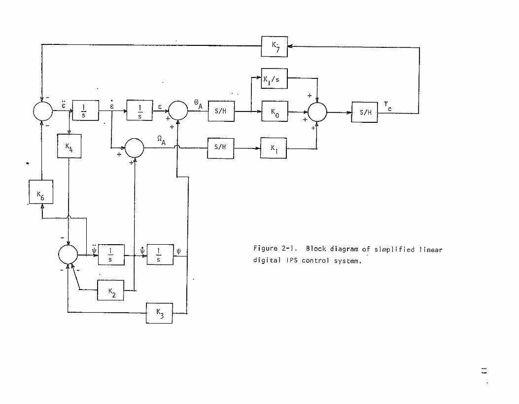
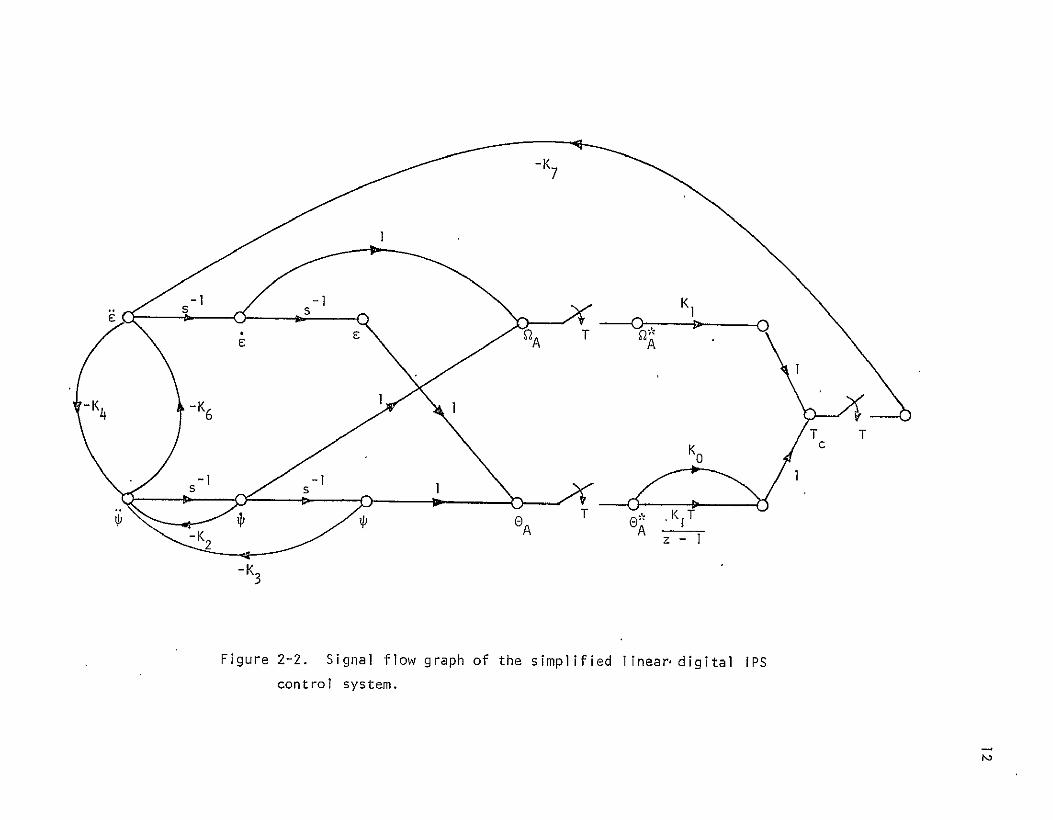


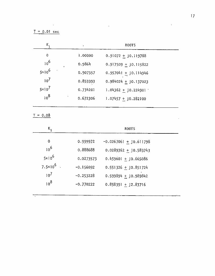
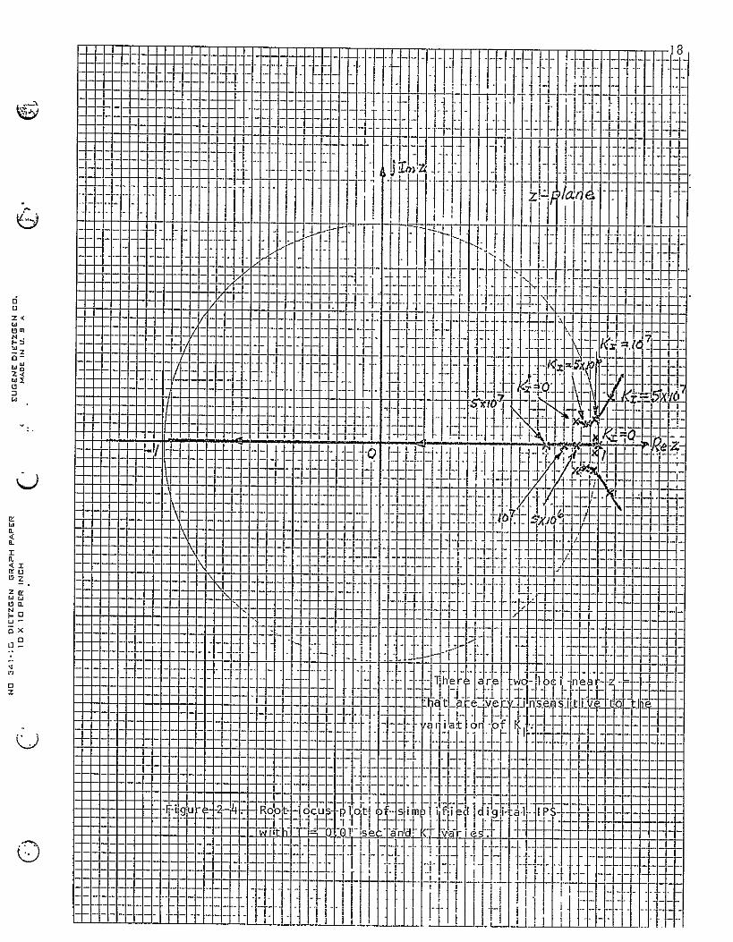


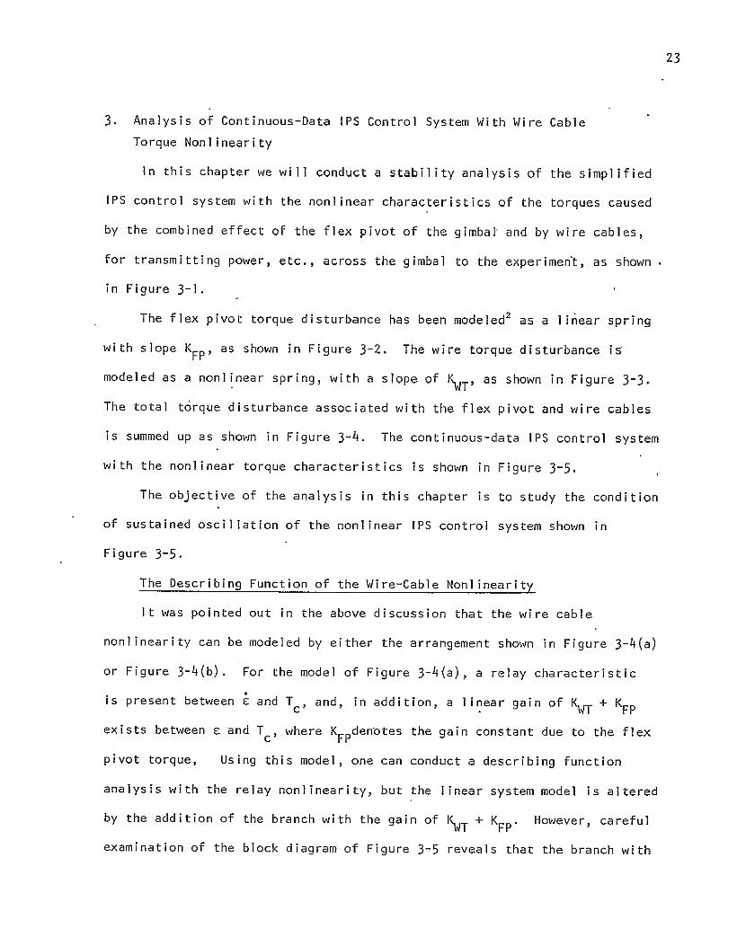


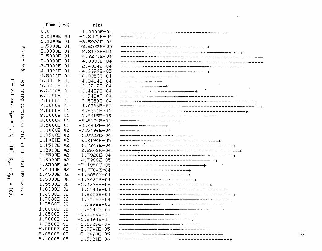


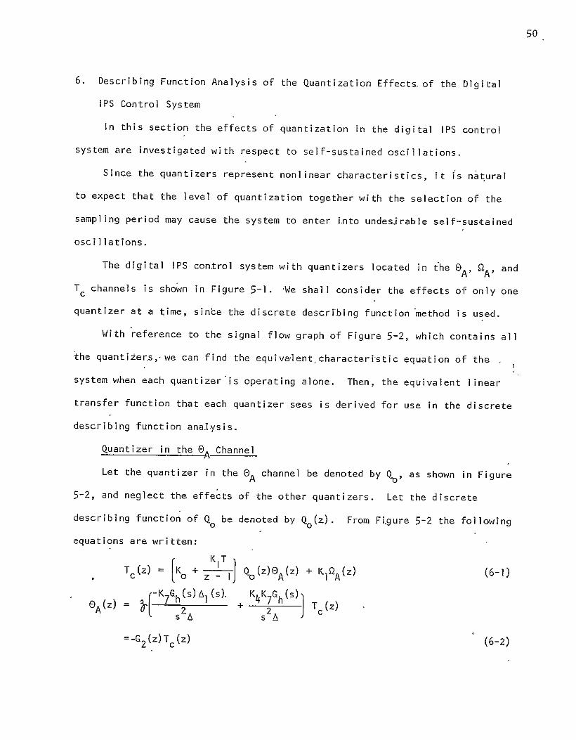


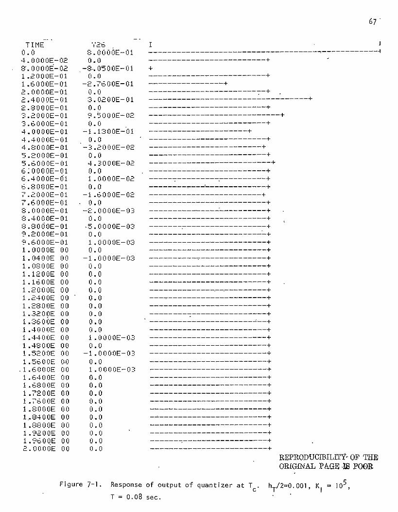

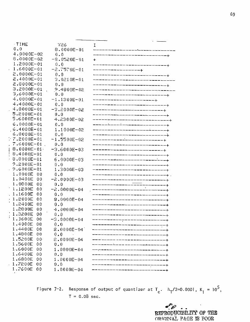


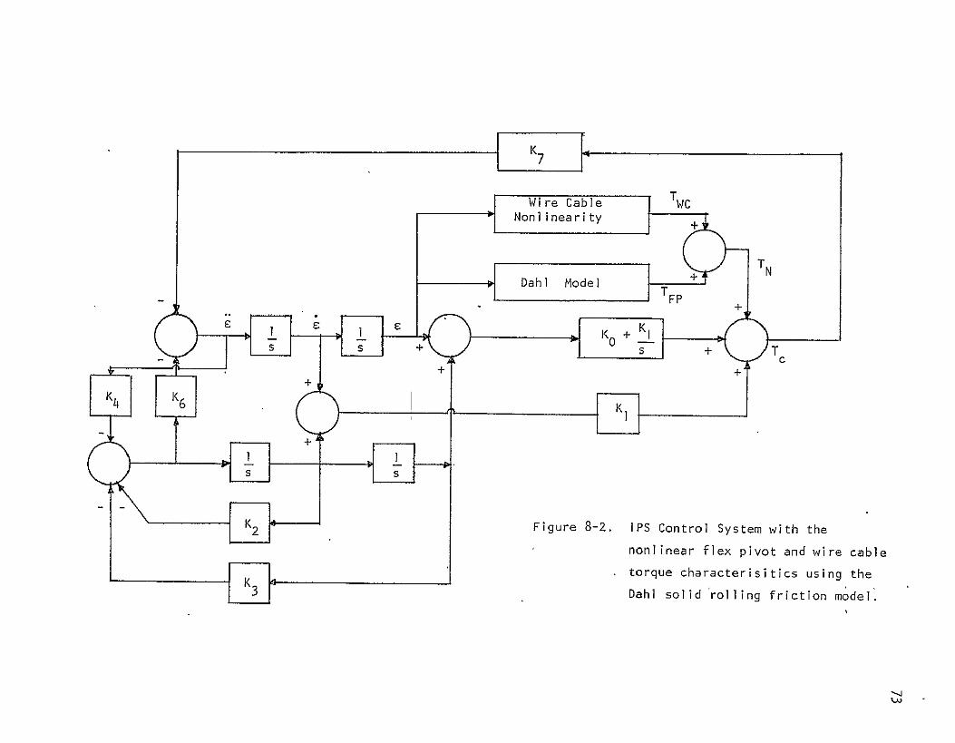
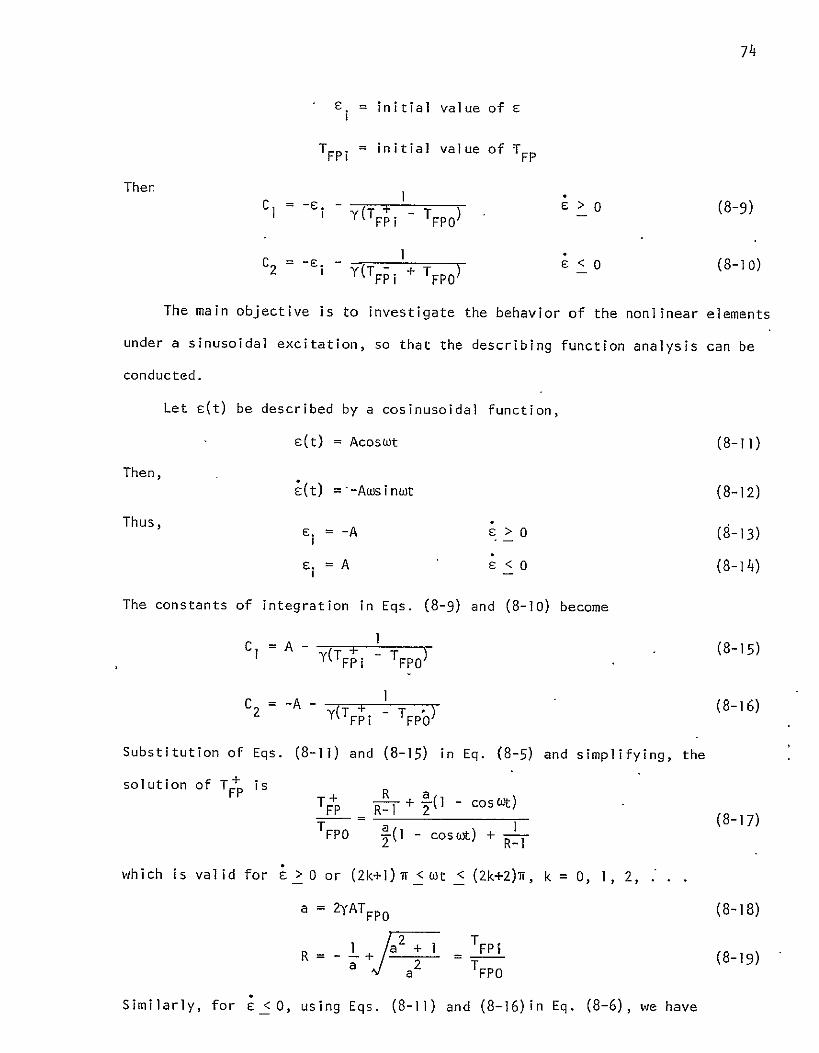


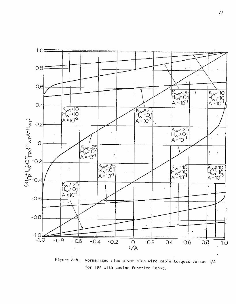


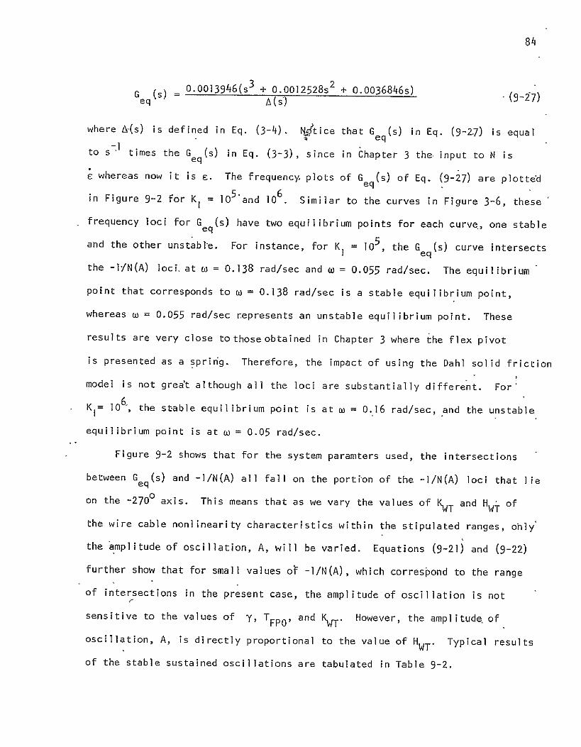
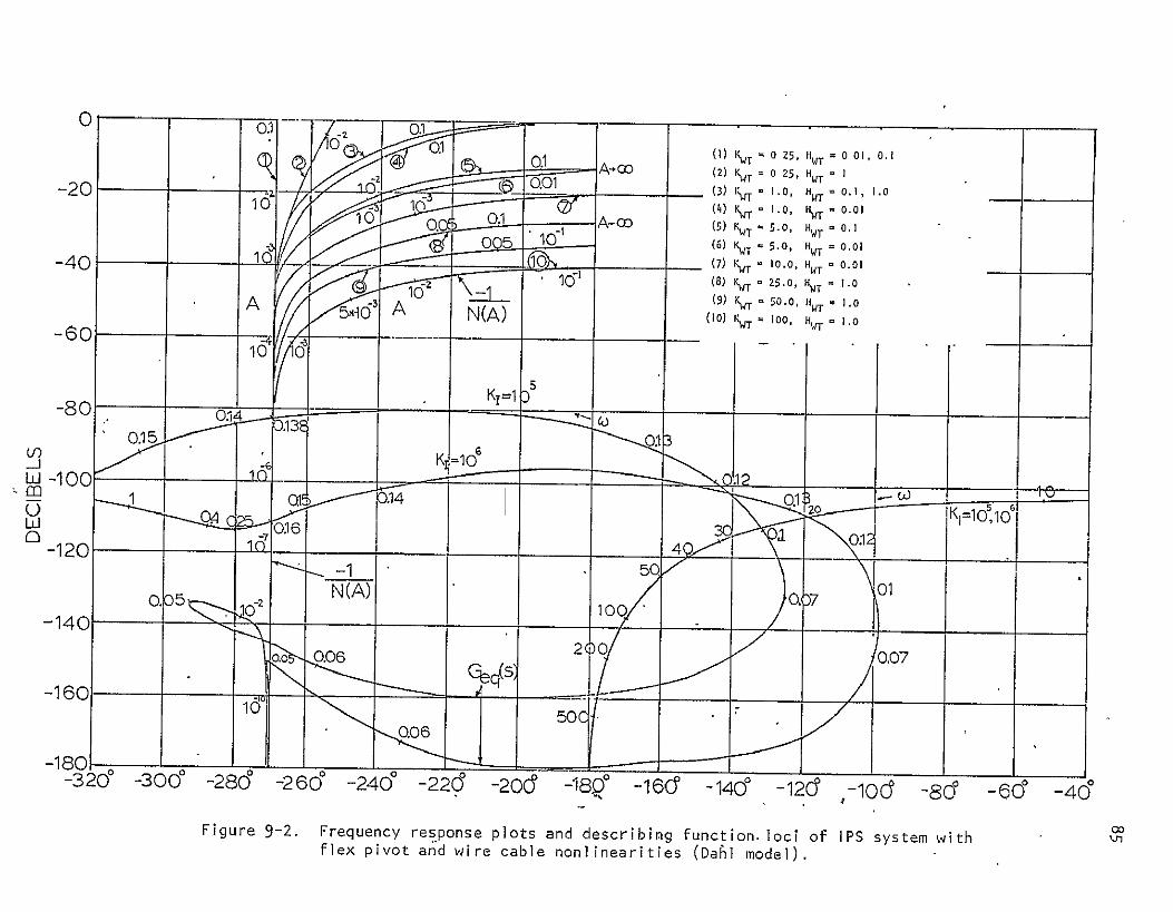


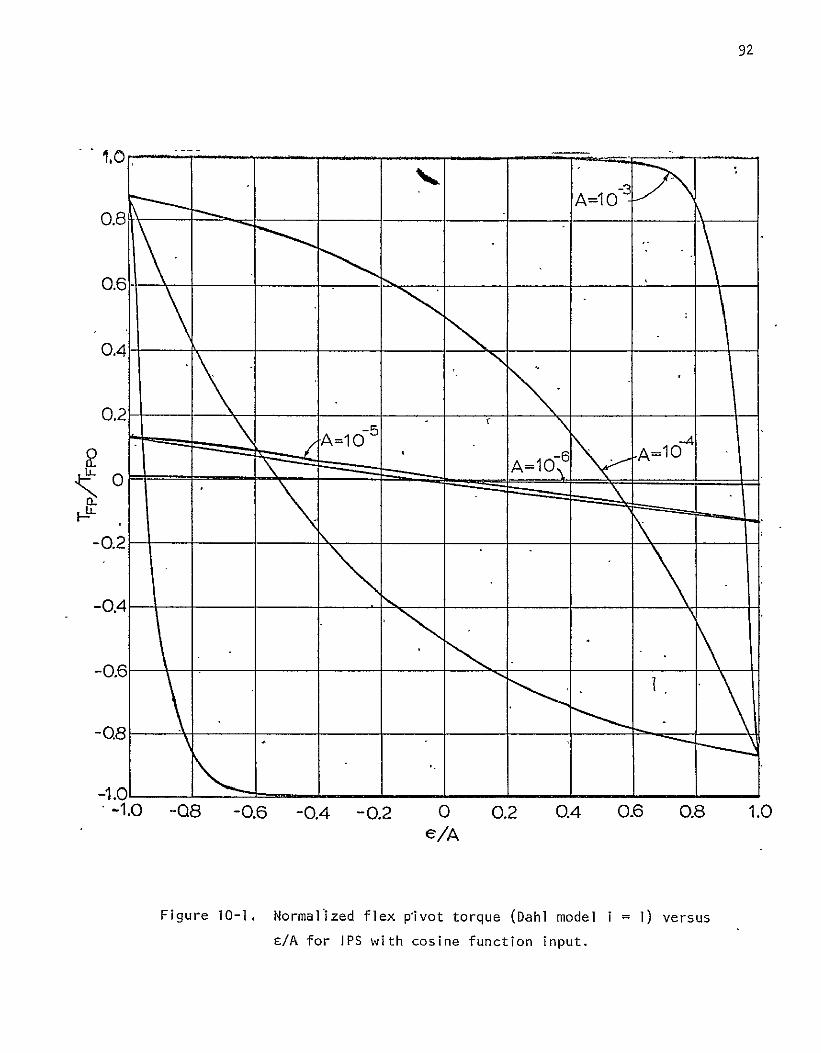


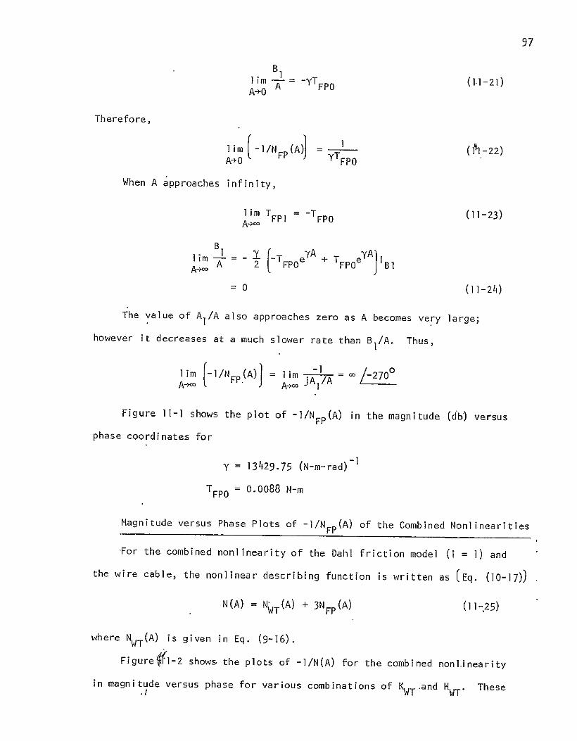
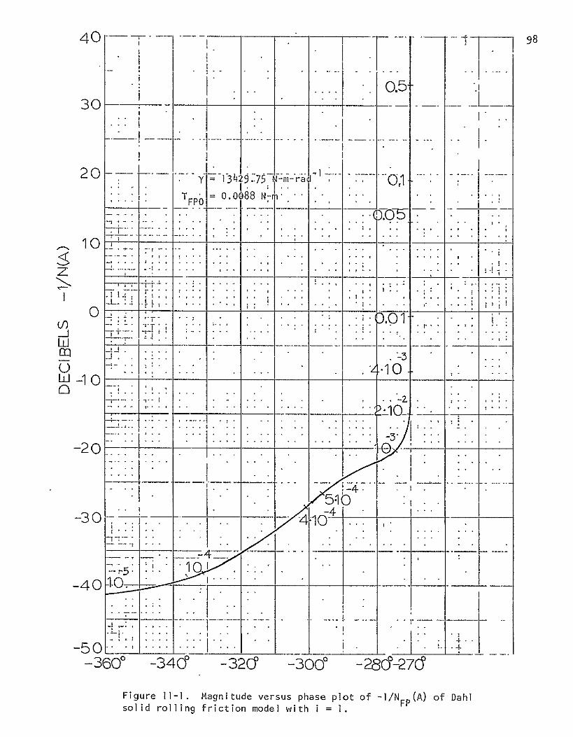


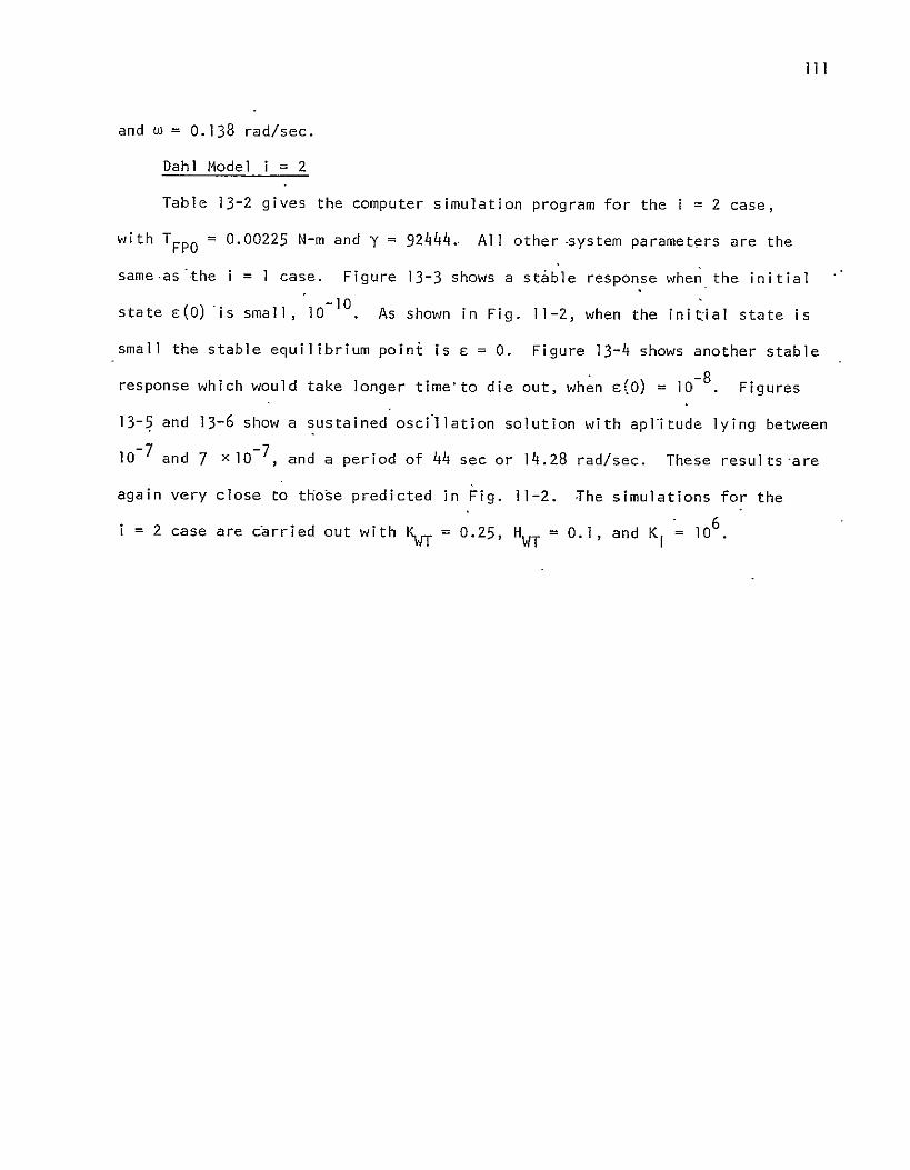


![Sizes Payload Compensation path XY up to 20 kg - Comoso · Compensation path XY ... Material CR CR CR CR NBR CR CR CR CR CR CR NBR NBR NBR NBR NBR ... Bending [Nm/rad] 474 552 1025](https://img.dokumen.tips/doc/110x75/5af1b3557f8b9ac57a903b0d/sizes-payload-compensation-path-xy-up-to-20-kg-path-xy-material-cr-cr-cr-cr.jpg)