naMe: Unit 2 • Linear and exponentiaL reLationships …windrivermath.wikispaces.com/.../view/M1+Unit+2+Lesson+4.pdfLesson 2.4.1: Identifying Key Features of Linear and Exponential

Unit 2 • Linear and exponentiaL reLationshipsLesson 4: Interpreting Graphs of Functions

naMe:

Assessment

CCSS IP Math I Teacher Resource © Walch EducationU2-163

Pre-AssessmentCircle the letter of the best answer.

1. An online company charges $5 a month plus $2 for each movie you decide to download. Which of the following graphs best represents this scenario?

a.

0 1 2 3 4 5 6 7 8 9 10

2

4

6

8

10

12

14

16

18

20

22

24

Number of downloads

Tota

l cha

rges

($)

b.

0 1 2 3 4 5 6 7 8 9 10

2

4

6

8

10

12

14

16

18

20

22

24

Number of downloads

Tota

l cha

rges

($)

c.

0 1 2 3 4 5 6 7 8 9 10

2

4

6

8

10

12

14

16

18

20

22

24

Number of downloads

Tota

l cha

rges

($)

d.

0 1 2 3 4 5 6 7 8 9 10

2

4

6

8

10

12

14

16

18

20

22

24

Number of downloads

Tota

l cha

rges

($)

continued


naMe:

Assessment

CCSS IP Math I Teacher Resource U2-164

© Walch Education

2. The graph below can be described as:

-20 -18 -16 -14 -12 -10 -8 -6 -4 -20 2 4 6 8 10 12 14 16 18 20

-20

-18

-16

-14

-12

-10

-8

-6

-4

-2

2

4

6

8

10

12

14

16

18

20

a. a positive function that is increasing

b. a negative function that is decreasing

c. a positive function that is decreasing

d. a negative function that is increasing

continued


naMe:

Assessment


3. Use the table below to determine the rate of change for the interval [1, 5].

Weeks (x) Amount saved in dollars (f(x))1 162 383 604 825 104

a. $17.60 per week

b. $88 per week

c. $0.05 per week

d. $22 per week

4. Use the table below to determine the approximate rate of change for the interval [0, 3].

Years (x) Amount invested in dollars (f(x))0 1000.001 1060.902 1125.513 1194.054 1266.77

a. –$64.68 per year

b. $64.68 per year

c. $0.02 per year

d. The rate of change cannot be determined.

continued


naMe:

Assessment


© Walch Education

5. Use the graph below to determine the approximate rate of change for the interval [0, 30].

0 5 10 15 20 25 30 35 40 45 50

5

10

15

20

25

30

35

40

45

50

55

60

65

70

75

a. –2.4

b. 2.4

c. –0.42

d. The rate of change cannot be determined.

Lesson 4: Interpreting Graphs of Functions

Unit 2 • Linear and exponentiaL reLationships

Instruction


Common Core State Standards

F–IF.4 For a function that models a relationship between two quantities, interpret key features of graphs and tables in terms of the quantities, and sketch graphs showing key features given a verbal description of the relationship. Key features include: intercepts; intervals where the function is increasing, decreasing, positive, or negative; relative maximums and minimums; symmetries; end behavior; and periodicity. ★

F–IF.5 Relate the domain of a function to its graph and, where applicable, to the quantitative relationship it describes. For example, if the function h(n) gives the number of person-hours it takes to assemble n engines in a factory, then the positive integers would be an appropriate domain for the function. ★

F–IF.6 Calculate and interpret the average rate of change of a function (presented symbolically or as a table) over a specified interval. Estimate the rate of change from a graph. ★

F–LE.1 Distinguish between situations that can be modeled with linear functions and with exponential functions. ★

a. Prove that linear functions grow by equal differences over equal intervals, and that exponential functions grow by equal factors over equal intervals.

b. Recognize situations in which one quantity changes at a constant rate per unit interval relative to another.

c. Recognize situations in which a quantity grows or decays by a constant percent rate per unit interval relative to another.

Essential Questions

1. How can maximum and minimum values of a function be applied to a real-world context?

2. What is the purpose of using the rate of change to analyze real-world data?

3. For what types of real-world data can you find the rate of change?

4. Why might you find the rate of change?

WORDS TO KNOW

asymptote a line that a graph gets closer and closer to, but never crosses or touches

continuous having no breaks


Instruction


© Walch Education

domain the set of all inputs of a function

extrema the minima and maxima of a function

integer a number that is not a fraction or a decimal

intercept the point at which a line intersects the x- or y-axis

interval a continuous series of values

irrational numbers numbers that cannot be written as a

b, where a and b are integers and

b ≠ 0; any number that cannot be written as a decimal that ends or repeats

natural numbers the set of positive integers {1, 2, 3, ..., n}

negative function a portion of a function where the y-values are less than 0 for all x-values

positive function a portion of a function where the y-values are greater than 0 for all x-values

rate of change a ratio that describes how much one quantity changes with respect to the change in another quantity; also known as the slope of a line

ratio the relation between two quantities; can be expressed in words, fractions, decimals, or as a percent

rational number a number that can be written as a

b, where a and b are integers and b ≠ 0;

any number that can be written as a decimal that ends or repeats

real numbers the set of all rational and irrational numbers

relative maximum the greatest value of a function for a particular interval of the function

relative minimum the least value of a function for a particular interval of the function

slope the measure of the rate of change of one variable with respect to another

variable; y y

x x

y

x=

−−

= =sloperise

run2 1

2 1

slope-intercept method the method used to graph a linear equation; with this method, draw a line using only two points on the coordinate plane

undefined slope the slope of a vertical line

whole numbers the set of natural numbers that also includes 0: {0, 1, 2, 3, ...}

x-intercept the point at which the line intersects the x-axis at (x, 0)


Instruction


Recommended Resources• National Council of Teachers of Mathematics. “Changing Cost per Minute.”

http://walch.com/rr/CAU3L3ChangingCost

This interactive graphical representation of cell phone charges allows users to view how changing the graph of the cost per minute affects the graph of the total cost.

• National Council of Teachers of Mathematics. “Constant Cost per Minute.”

http://walch.com/rr/CAU3L3ConstantCost

This interactive graphical representation of cell phone charges allows users to view how the total cost of service changes when a constant cost per minute is manipulated.

• Oswego City School District Regents Exam Prep Center. “Exponential Growth and Decay.”

http://walch.com/rr/CAU3L3ExponentialDecay

This site summarizes exponential growth and decay using various examples to describe the key features of graphs including rates of change.


naMe:


© Walch Education

Lesson 2.4.1: Identifying Key Features of Linear and Exponential Graphs

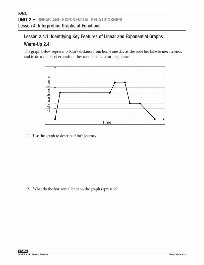
Warm-Up 2.4.1The graph below represents Kim’s distance from home one day as she rode her bike to meet friends and to do a couple of errands for her mom before returning home.

-10 1 2 3 4 5 6 7 8 9 10 11 12 13 14 15 16 17 18 19 20 21

1

2

3

4

5

6

7

8

9

Dis

tanc

e fr

om h

ome

Time

1. Use the graph to describe Kim’s journey.

2. What do the horizontal lines on the graph represent?


Instruction


Lesson 2.4.1: Identifying Key Features of Linear and Exponential GraphsCommon Core State Standards

F–IF.4 For a function that models a relationship between two quantities, interpret key features of graphs and tables in terms of the quantities, and sketch graphs showing key features given a verbal description of the relationship. Key features include: intercepts; intervals where the function is increasing, decreasing, positive, or negative; relative maximums and minimums; symmetries; end behavior; and periodicity. ★

F–IF.5 Relate the domain of a function to its graph and, where applicable, to the quantitative relationship it describes. For example, if the function h(n) gives the number of person-hours it takes to assemble n engines in a factory, then the positive integers would be an appropriate domain for the function. ★

Warm-Up 2.4.1 DebriefThe graph below represents Kim’s distance from home one day as she rode her bike to meet friends and to do a couple of errands for her mom before returning home.

-10 1 2 3 4 5 6 7 8 9 10 11 12 13 14 15 16 17 18 19 20 21

1

2

3

4

5

6

7

8

9

Dis

tanc

e fr

om h

ome

Time

1. Use the graph to describe Kim’s journey.

Answers will vary. One possible response: Kim rode her bike to her friend’s house. She stayed at her friend’s house for a while. Then she left her friend’s house and rode to a store, which is even farther away from her house. She stayed at the store for a short time and bought a couple of items. Kim then headed back toward her house, stopping once more to take a picture of a beautiful statue along the way. She then biked the rest of the way back home.

2. What do the horizontal lines represent in the graph?

The horizontal lines represent times when Kim stayed at one location. Her distance from home did not change, but time continued to pass.


Instruction


© Walch Education

Connection to the Lesson

• Students will extend their understanding of graphs and begin to more formally describe various features.

• Students will be asked to interpret key features from graphs and tables as well as sketch graphs given a verbal description.


Instruction


Prerequisite Skills

This lesson requires the use of the following skills:

• graphing a linear function from a table or equation

• graphing an exponential function from a table or equation

• having knowledge of function notation, domain, and independent and dependent variables

IntroductionReal-world contexts that have two variables can be represented in a table or graphed on a coordinate plane. There are many characteristics of functions and their graphs that can provide a great deal of information. These characteristics can be analyzed and the real-world context can be better understood.

Key Concepts

• One of the first characteristics of a graph that we can observe are the intercepts, where a function crosses the x-axis and y-axis.

• The y-intercept is the point at which the graph crosses the y-axis, and is written as (0, y).

• The x-intercept is the point at which the graph crosses the x-axis, and is written as (x, 0).

-10 -9 -8 -7 -6 -5 -4 -3 -2 -1 0 1 2 3 4 5 6 7 8 9 10

-10

-9

-8

-7

-6

-5

-4

-3

-2

-1

1

2

3

4

5

6

7

8

9

10

x-intercept (4, 0)

-10 -9 -8 -7 -6 -5 -4 -3 -2 -1 0 1 2 3 4 5 6 7 8 9 10

-10

-9

-8

-7

-6

-5

-4

-3

-2

-1

1

2

3

4

5

6

7

8

9

10

y-intercept (0, -8)


Instruction


© Walch Education

-10 -9 -8 -7 -6 -5 -4 -3 -2 -1 0 1 2 3 4 5 6 7 8 9 10

-10

-9

-8

-7

-6

-5

-4

-3

-2

-1

1

2

3

4

5

6

7

8

9

10

x-intercept (2, 0)

-10 -9 -8 -7 -6 -5 -4 -3 -2 -1 0 1 2 3 4 5 6 7 8 9 10

-10

-9

-8

-7

-6

-5

-4

-3

-2

-1

1

2

3

4

5

6

7

8

9

10

y-intercept (0, -3)

• Another characteristic of graphs that we can observe is whether the graph represents a function that is increasing or decreasing.

• When determining whether intervals are increasing or decreasing, focus just on the y-values.

• Begin by reading the graph from left to right and notice what happens to the graphed line. If the line goes up from left to right, then the function is increasing. If the line is going down from left to right, then the function is decreasing.

• A function is said to be constant if the graphed line is horizontal, neither rising nor falling.

-10 -9 -8 -7 -6 -5 -4 -3 -2 -1 0 1 2 3 4 5 6 7 8 9 10

-10

-9

-8

-7

-6

-5

-4

-3

-2

-1

1

2

3

4

5

6

7

8

9

10

Decreasing

-10 -9 -8 -7 -6 -5 -4 -3 -2 -1 0 1 2 3 4 5 6 7 8 9 10

-10

-9

-8

-7

-6

-5

-4

-3

-2

-1

1

2

3

4

5

6

7

8

9

10

Increasing


Instruction


-10 -9 -8 -7 -6 -5 -4 -3 -2 -1 0 1 2 3 4 5 6 7 8 9 10

-10

-9

-8

-7

-6

-5

-4

-3

-2

-1

1

2

3

4

5

6

7

8

9

10 Increasing

-10 -9 -8 -7 -6 -5 -4 -3 -2 -1 0 1 2 3 4 5 6 7 8 9 10

-10

-9

-8

-7

-6

-5

-4

-3

-2

-1

1

2

3

4

5

6

7

8

9

10 Decreasing

• An interval is a continuous series of values. (Continuous means “having no breaks.”) A function is positive on an interval if the y-values are greater than zero for all x-values in that interval.

• A function is positive when its graph is above the x-axis.

• Begin by looking for the x-intercepts of the function.

• Write the x-values that are greater than zero using inequality notation.

• A function is negative on an interval if the y-values are less than zero for all x-values in that interval.

• The function is negative when its graph is below the x-axis.

• Again, look for the x-intercepts of the function.

• Write the x-values that are less than zero using inequality notation.


Instruction


© Walch Education

-10 -9 -8 -7 -6 -5 -4 -3 -2 -1 0 1 2 3 4 5 6 7 8 9 10

-10

-9

-8

-7

-6

-5

-4

-3

-2

-1

1

2

3

4

5

6

7

8

9

10

The function is positive when x > 4.

-10 -9 -8 -7 -6 -5 -4 -3 -2 -1 0 1 2 3 5 6 7 8 9 104

-10

-9

-8

-7

-6

-5

-4

-3

-2

-1

1

2

3

4

5

6

7

8

9

10

The function is negativewhen x < 4.

-10 -9 -8 -7 -6 -5 -4 -3 -2 -1 0 1 2 3 4 5 6 7 8 9 10

-10

-9

-8

-7

-6

-5

-4

-3

-2

-1

1

2

3

4

5

6

7

8

9

10


-10 -9 -8 -7 -6 -5 -4 -3 -2 -1 0 1 2 3 4 5 6 7 8 9 10

-10

-9

-8

-7

-6

-5

-4

-3

-2

-1

1

2

3

4

5

6

7

8

9

10

The function is negativewhen x < 2.

• Graphs may contain extrema, or minimum or maximum points.

• A relative minimum is the point that is the lowest, or the y-value that is the least for a particular interval of a function.

• A relative maximum is the point that is the highest, or the y-value that is the greatest for a particular interval of a function.

• Linear and exponential functions will only have a relative minimum or maximum if the domain is restricted.

• The domain of a function is the set of all inputs, or x-values of a function.


Instruction


• Compare the following two graphs. The graph on the left is of the function f(x) = 2x – 8. The graph on the right is of the same function, but the domain is for x ≥ 1. The minimum of the function is –6.

-10 -9 -8 -7 -6 -5 -4 -3 -2 -1 0 1 2 3 4 5 6 7 8 9 10

-10

-9

-8

-7

-6

-5

-4

-3

-2

-1

1

2

3

4

5

6

7

8

9

10

1 Minimum at –6No maximum

-10 -9 -8 -7 -6 -5 -4 -3 -2 -1 0 1 2 3 4 5 6 7 8 9 10

-10

-9

-8

-7

-6

-5

-4

-3

-2

-1

1

2

3

4

5

6

7

8

9

10

No minimumNo maximum

• Functions that represent real-world scenarios often include domain restrictions. For example, if we were to calculate the cost to download a number of e-books, we would not expect to see negative or fractional downloads as values for x.

• There are several ways to classify numbers. The following table lists the most commonly used classifications when defining domains.

Natural numbers 1, 2, 3, ...

Whole numbers 0, 1, 2, 3, ...

Integers ..., –3, –2, –1, 0, 1, 2, 3, ...

Rational numbers numbers that can be written as a


b ≠ 0; any number that can be written as a decimal that ends or repeats

Irrational numbers numbers that cannot be written as a


b ≠ 0; any number that cannot be written as a decimal that ends or

repeats

Real numbers the set of all rational and irrational numbers


Instruction


© Walch Education

• An exponential function in the form f(x) = ax, where a > 0 and a ≠ 1, has an asymptote, or a line that the graph gets closer and closer to, but never crosses or touches.

• The function in the following graph has a horizontal asymptote at y = –4.

• It may appear as though the graphed line touches y = –4, but it never does.

-10 -9 -8 -7 -6 -5 -4 -3 -2 -1 0 1 2 3 4 5 6 7 8 9 10

-10

-9

-8

-7

-6

-5

-4

-3

-2

-1

1

2

3

4

5

6

7

8

9

10

Asymptote

• Fairly accurate representations of functions can be sketched using the key features we have just described.

Common Errors/Misconceptions

• believing that exponential functions will eventually touch or intersect an asymptote

• incorrectly identifying the type of function as either exponential or linear

• misidentifying key features on a graph

• incorrectly choosing the domain for a function


Instruction


Guided Practice 2.4.1Example 1

A taxi company in Atlanta charges $2.75 per ride plus $1.50 for every mile driven. Determine the key features of this function.

0 1 2 3 4 5 6 7 8 9 10

1

2

3

4

5

6

7

8

9

10

Miles traveled

Cost

in d

olla

rs

1. Identify the type of function described.

We can see by the graph that the function is increasing at a constant rate.

The function is linear.

2. Identify the intercepts of the graphed function.

The graphed function crosses the y-axis at the point (0, 2.75).

The y-intercept is (0, 2.75).

The function does not cross the x-axis.

There is not an x-intercept.


Instruction


© Walch Education

3. Determine whether the graphed function is increasing or decreasing.

Reading the graph left to right, the y-values are increasing.

The function is increasing.

4. Determine where the function is positive and negative.

The y-values are positive for all x-values greater than 0.


The y-values are never negative in this scenario.

The function is never negative.

5. Determine the relative minimum and maximum of the graphed function.

The lowest y-value of the function is 2.75. This is shown with the closed dot at the coordinate (0, 2.75).

The relative minimum is 2.75.

The values increase infinitely; therefore, there is no relative maximum.

6. Identify the domain of the graphed function.

The lowest x-value is 0 and it increases infinitely.

x can be any real number greater than or equal to 0.

The domain can be written as x ≥ 0.

7. Identify any asymptotes of the graphed function.

The graphed function is a linear function, not an exponential; therefore, there are no asymptotes for this function.


Instruction


Example 2

A pendulum swings to 90% of its height on each swing and starts at a height of 80 cm. The height of the pendulum in centimeters, y, is recorded after x number of swings. Determine the key features of this function.

Number of swings (x) Height in cm (y)0 801 722 64.83 58.325 47.24

10 27.8920 9.7340 1.1860 0.1480 0.02


The scenario described here is that of an exponential function.

We can be certain of this because the pendulum swings at 90% of its height in each swing; also, we can see from the table that the values for y do not decrease at a constant rate.

2. Identify the intercepts of the function based on the information in the table.

The function crosses the y-axis at the point (0, 80) as indicated in the table.

The y-intercept is (0, 80).

As the x-values increase, the y-values get closer and closer to 0, but do not seem to reach 0; therefore, there is not an x-intercept.


Instruction


© Walch Education

3. Determine whether the function is increasing or decreasing.

As the x-values increase, the y-values decrease.

The function is decreasing.


The y-values are positive for all x-values greater than 0.




5. Determine the relative minimum and maximum of the function.

The data in the table do not change at a constant rate; therefore, the function is not linear.

Based on the information given in the problem and the values in the table, we know that this is an exponential function.

Exponential functions do not have a relative minimum because the graph continues to become infinitely smaller.

The height of the pendulum never goes higher than its initial height; therefore, the relative maximum of this function is (0, 80).

6. Identify the domain of the function.

The lowest x-value is 0 and it increases infinitely.

x can be any real number greater than or equal to 0, but cannot be a partial swing.

The domain is all whole numbers.

7. Identify any asymptotes of the function.

The points approach 0, but never actually reach 0.

The asymptote of this function is y = 0.


Instruction


Example 3

A ringtone company charges $15 a month plus $2 for each ringtone downloaded. Create a graph and then determine the key features of this function.

1. Create a function to represent this scenario.

Let x represent the number of ringtones downloaded and f(x) represent the total monthly fee.

f(x) = 15 + 2x

2. Graph the function.

When creating the graph of the function, consider the domain of the function.

In past lessons, we have graphed the equations of functions. In this lesson, and in the future, we want to consider the function as it relates to the scenario.

We can’t download a partial ringtone, and can’t be charged for a partial download.

It does not make sense to consider values for x other than those that are whole numbers.

(continued)


Instruction


© Walch Education

Notice the points in the graph are not connected.

0 1 2 3 4 5 6 7 8 9 10

2

4

6

8

10

12

14

16

18

20

22

24

26

28

30

32

34

36

38

Ringtones downloaded

Fee

in d

olla

rs ($

)


The function is still a linear function; it just has a restricted domain. We can see this in the function f(x) = 15 + 2x and in the graph of the function.


Instruction


4. Identify the intercepts of the graphed function.

The graphed function crosses the y-axis at the point (0, 15).

The y-intercept is (0, 15).

The function does not cross the x-axis.

There is no x-intercept.

5. Determine whether the graphed function is increasing or decreasing.

Reading the graph left to right, the y-values are increasing.

The function is increasing.


The y-values are positive for all x-values greater than or equal to 0.

The function is positive when x ≥ 0.



7. Determine the relative minimum and maximum of the graphed function.

The lowest y-value of the function is 15. This is shown with the dot at the coordinate (0, 15).

The relative minimum is 15.

The x-values increase infinitely; therefore there is not a relative maximum.


Instruction


© Walch Education

8. Identify the domain of the graphed function.

The lowest x-value is 0 and it increases infinitely, but for only whole-number values.

x can be any whole number greater than or equal to 0.

9. Identify any asymptotes of the graphed function.

The graphed function is a linear function, not an exponential; therefore, there are no asymptotes for this function.


naMe:


Problem-Based Task 2.4.1: Careful CalculationsThere are many things to think about when purchasing a new car: year, make, model, included options, and price. As important as these considerations are, it is also important to consider the decreasing value of the car over time.

Use the following key features to graph the value of a car over time:

• The average price of a car in the United States is approximately $30,750.

• The value decreases each year at an exponential rate and approaches the asymptote of y = 0.

• The average car loses nearly half its original value after 5 years.

For what values of x is the graph positive? What is the domain of this function? Identify the minimum and maximum of this graph.


naMe:


© Walch Education

Problem-Based Task 2.4.1: Careful Calculations

Coachinga. What is the independent variable?

b. What is the minimum value of this variable?

c. What is the maximum value of this variable?

d. What is an appropriate scale for this variable?

e. What is the dependent variable?

f. What is the minimum value of this variable?

g. What is the maximum value of this variable?

h. What is an appropriate scale for this variable?

i. Is this situation modeled by a linear function or an exponential function?

j. How does the value after 5 years help you determine the shape of this graph?

k. Why does this graph have an asymptote of y = 0?

l. For what values of x is the graph positive?

m. Is the graph ever negative? Why or why not?

n. What is the minimum of this graph?

o. What is the maximum of this graph?

p. What is the domain of this function?


Instruction


Problem-Based Task 2.4.1: Careful Calculations

Coaching Sample Responsesa. What is the independent variable?

The independent variable is the number of years.

b. What is the minimum value of this variable?

The minimum value of this variable is 0.

c. What is the maximum value of this variable?

There is not a maximum value because the number of years continues forever.

d. What is an appropriate scale for this variable?

An appropriate scale for this variable could be 0 to 20 in increments of 1. 20 years is longer than most people would consider the value of a car.

e. What is the dependent variable?

The dependent variable is the value of the car in dollars.

f. What is the minimum value of this variable?

The minimum value of this variable is 0.

g. What is the maximum value of this variable?

The maximum value of this variable is 30,750.

h. What is an appropriate scale for this variable?

An appropriate scale for this variable would need to be from 0 to at least 30,750. It would be advisable to count by 2,000 or 2,500 in order to maintain a readable graph.

i. Is this situation modeled by a linear function or an exponential function?

This situation is modeled by an exponential function. We are told in the description that the value decreases exponentially.

j. How does the value after 5 years help you determine the shape of this graph?

The value after 5 years gives us a place to mark another point. We know the graph is going to curve toward the x-axis. This gives us one more point to go through in order to create a more accurate graph.

k. Why does this graph have an asymptote of y = 0?

The value of the car will never be $0. The car may not be worth much, but it will always be worth something.


Instruction


© Walch Education

l. For what values of x is the graph positive?

The graph is positive for all x-values greater than or equal to 0, or x ≥ 0.

m. Is the graph ever negative? Why or why not?

The graph is never negative because the value of the car is never negative.

n. What is the minimum of this graph?

There is no minimum because the graph is an exponential function.

o. What is the maximum of this graph?

The maximum of the graph occurs at the point (0, 30,750).

p. What is the domain of this function?

The domain of this function is all real numbers greater than or equal to 0, or where x ≥ 0.

0 2 4 6 8 10 12 14 16 18 20

2

4

6

8

10

12

14

16

18

20

22

24

26

28

30

Years

Valu

e of

car

(tho

usan

ds o

f dol

lars

)

Recommended Closure Activity

Select one or more of the essential questions for a class discussion or as a journal entry prompt.


naMe:


Practice 2.4.1: Identifying Key Features of Linear and Exponential GraphsDetermine the domain of each function, and then graph the function on graph paper.

1. Mikhail receives a base weekly salary of $350 plus a commission of $50 for each vacuum he sells. His weekly earnings can be modeled by the function f(x) = 50x + 350.

2. A population of insects begins with 15 insects and doubles every month. The population can be modeled by the function f(x) = 15(2)x.

Determine the key features of each function. Include the x- and y-intercepts, whether the function is increasing or decreasing, whether it’s negative or positive, the minimum and maximum, asymptotes, and domain. Find the asymptotes as if the domain were all real numbers.

3. You and your friends are out hiking. You start the hike with 50 pounds of food for the group, and eat about 7 pounds each day. Identify the key features of the graph of this function.

0 1 2 3 4 5 6 7 8 9 10

2

4

6

8

10

12

14

16

18

20

22

24

26

28

30

32

34

36

38

40

42

44

46

48

50

Days

Poun

ds o

f foo

d

continued


naMe:


© Walch Education

4. Mason borrowed $1,200 from a friend to buy a new hot tub. His friend doesn’t charge any interest and Mason makes $50 payments each month. Identify the key features of the graph of this function.

0 2 4 6 8 10 12 14 16 18 20 22 24

50

100

150

200

250

300

350

400

450

500

550

600

650

700

750

800

850

900

950

1000

1050

1100

1150

1200

Months

Am

ount

ow

ed ($

)

continued


naMe:


5. A gear on a machine turns at a rate of 3 revolutions per second. Identify the key features of the graph of this function.

0 1 2 3 4 5 6 7 8 9 10

2

4

6

8

10

12

14

16

18

20

22

24

26

28

30

Time (seconds)

Num

ber o

f rev

olut

ions

6. The cost of an air conditioner is $110. The cost to run the air conditioner is $0.35 per minute. Identify the key features of this function.

Minutes (x) Cost in dollars (f(x))0 110.00

30 120.5060 131.0090 141.50

120 152.00continued


naMe:


© Walch Education

7. A stock is declining at a rate of 70% of its value every 2 weeks. The stock started at $300. Identify the key features of the graph of this function.

0 2 4 6 8 10 12 14 16 18

25

50

75

100

125

150

175

200

225

250

275

300

Weeks

Stoc

k w

orth

($)

continued


naMe:


8. A wildflower species triples in 4 days. A field started with 9 wildflowers in the early spring. Identify the key features of the graph of this function.

0 2 4 6 8 10 12 14 16 18

50

100

150

200

250

300

350

400

450

500

550

600

650

700

750

800

850

900

950

Days

Wild

�ow

ers

continued


naMe:


© Walch Education

9. An investment of $1,200 earns 3.9% interest and is compounded semi-annually. Identify the key features of the graph of this function.

0 2 4 6 8 10 12 14 16 18 20

250

500

750

1000

1250

1500

1750

2000

2250

2500

2750

Years

Inve

stm

ent w

orth

($)

10. An investment of $3,000 earns 1.5% interest and is compounded weekly. Identify the key features of this function.

Year (x) Investment value in dollars (f(x))0 30001 3045.582 3091.843 3138.824 3186.505 3234.916 3281.06


naMe:


Lesson 2.4.2: Proving Average Rate of Change

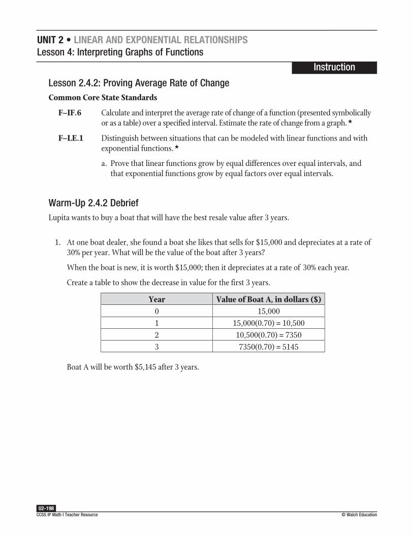
Warm-Up 2.4.2Lupita wants to buy a boat that will have the best resale value after 3 years.

1. At one boat dealer, she found a boat she likes that sells for $15,000 and depreciates at a rate of 30% per year. What will be the value of the boat after 3 years?

2. At another dealer, she found a boat that costs $12,000 and depreciates at a rate of 20% per year. What will be the value of the boat after 3 years?

3. Which boat will have the greater value in 3 years?


Instruction


© Walch Education

Lesson 2.4.2: Proving Average Rate of ChangeCommon Core State Standards



a. Prove that linear functions grow by equal differences over equal intervals, and that exponential functions grow by equal factors over equal intervals.

Warm-Up 2.4.2 DebriefLupita wants to buy a boat that will have the best resale value after 3 years.

1. At one boat dealer, she found a boat she likes that sells for $15,000 and depreciates at a rate of 30% per year. What will be the value of the boat after 3 years?

When the boat is new, it is worth $15,000; then it depreciates at a rate of 30% each year.

Create a table to show the decrease in value for the first 3 years.

Year Value of Boat A, in dollars ($)0 15,0001 15,000(0.70) = 10,5002 10,500(0.70) = 73503 7350(0.70) = 5145

Boat A will be worth $5,145 after 3 years.


Instruction


2. At another dealer, she found a boat that costs $12,000 and depreciates at a rate of 20% per year. What will be the value of the boat after 3 years?

When the boat is new, it is worth $12,000; then it depreciates at a rate of 20% each year.

Create a table to show the decrease in value for the first 3 years.

Year Value of Boat B, in dollars ($)0 12,0001 12,000(0.80) = 96002 9600(0.80) = 76803 7680(0.80) = 6144

Boat B will be worth $6,144 after 3 years.

3. Which boat will have the greater value in 3 years?

Boat A will be worth $5,145 after 3 years.

Boat B will be worth $6,144 after 3 years.

Boat B will be worth more than Boat A after 3 years.


• Students will be asked to calculate the average rate of change of a function over a specified interval given a graph.

• Students will compare rates of change over various intervals.


Instruction


© Walch Education

Prerequisite Skills


• reading and interpreting data from charts and tables

• understanding slope

Introduction

In previous lessons, we have found the slope of linear equations and functions using the slope

formula, y y

x x

−−

2 1

2 1. We have also identified the slope of a line from a given equation by rewriting

the equation in slope-intercept form, y = mx + b, where m is the slope of the line. By calculating

the slope, we are able to determine the rate of change, or the ratio that describes how much one

quantity changes with respect to the change in another quantity of the function. The rate of change

can be determined from graphs, tables, and equations themselves. In this lesson, we will extend our

understanding of the slope of linear functions to that of intervals of exponential functions.

Key Concepts

• The rate of change is a ratio describing how one quantity changes as another quantity changes.

• Slope can be used to describe the rate of change.

• The slope of a line is the ratio of the change in y-values to the change in x-values.

• A positive rate of change expresses an increase over time.

• A negative rate of change expresses a decrease over time.

• Linear functions have a constant rate of change, meaning values increase or decrease at the same rate over a period of time.

• Not all functions change at a constant rate.

• The rate of change of an interval, or a continuous portion of a function, can be calculated.

• The rate of change of an interval is the average rate of change for that period.

• Intervals can be noted using the format [a, b], where a represents the initial x value of the interval and b represents the final x value of the interval. Another way to state the interval is a ≤ x ≤ b.


Instruction


• A function or interval with a rate of change of 0 indicates that the line is horizontal.

• Vertical lines have an undefined slope. An undefined slope is not the same as a slope of 0. This occurs when the denominator of the ratio is 0.

Calculating Rate of Change from a Table

1. Choose two points from the table.

2. Assign one point to be (x1, y

1) and the other point to be (x

2, y

2).

3. Substitute the values into the slope formula.

4. The result is the rate of change for the interval between the two points chosen.

• The rate of change between any two points of a linear function will be equal.

• The rate of change between any two points of any other function will not be equal, but will be an average for that interval.

Calculating Rate of Change from an Equation of a Linear Function

1. Transform the given linear function into slope-intercept form, f(x) = mx + b.

2. Identify the slope of the line as m from the equation.

3. The slope of the linear function is the rate of change for that function.

Calculating Rate of Change of an Interval from an Equation of an Exponential Function

1. Determine the interval to be observed.

2. Determine (x1, y

1) by identifying the starting x-value of the interval and substituting it

into the function.

3. Solve for y.

4. Determine (x2, y

2) by identifying the ending x-value of the interval and substituting it

into the function.

5. Solve for y.

6. Substitute (x1, y

1) and (x

2, y

2) into the slope formula to calculate the rate of change.

7. The result is the rate of change for the interval between the two points identified.


Instruction


© Walch Education


• incorrectly choosing the values of the indicated interval to calculate the rate of change

• substituting incorrect values into the formula for calculating the rate of change

• assuming the rate of change must remain constant over a period of time regardless of the function

• interpreting interval notation as coordinates


Instruction



Janie invests $1,300 at a rate of 2.6%, compounded monthly. The function that models this situation

is f xx

= +

( ) 1300 1

0.026

12

12

, where x represents time in years. What is the rate of change for the

interval [1, 4]?


The interval to be observed is [1, 4], or the interval where 1 ≤ x ≤ 4.

2. Determine (x1, y

1).

The initial x-value is 1.

Substitute the value 1 into the given function.

f xx

= +

( ) 1300 1

0.026

12

12

Given function

f = +

(1) 1300 1

0.026

12

12(1)

Substitute 1 for the value of x.

f = +

(1) 1300 1

0.026

12

12

Simplify as needed.

f(1) = 1300(1.002)12

f(1) ≈ 1334.21

(x1, y

1) is (1, 1334.21).


Instruction


© Walch Education

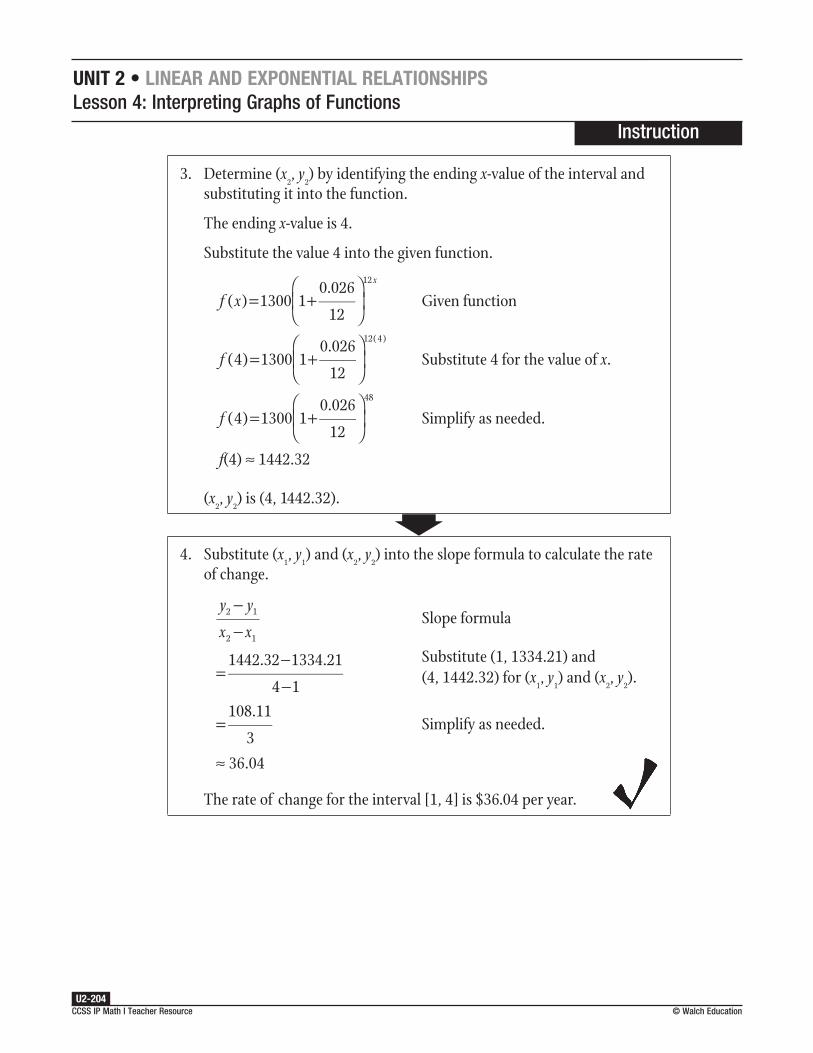
3. Determine (x2, y

2) by identifying the ending x-value of the interval and

substituting it into the function.

The ending x-value is 4.

Substitute the value 4 into the given function.

f xx

= +

( ) 1300 1

0.026

12

12

Given function

f = +

(4) 1300 1

0.026

12

12(4)

Substitute 4 for the value of x.

f = +

(4) 1300 1

0.026

12

48

Simplify as needed.

f(4) ≈ 1442.32

(x2, y

2) is (4, 1442.32).


1) and (x

2, y

2) into the slope formula to calculate the rate

of change.

y y

x x

−−

2 1

2 1

Slope formula

=−−

1442.32 1334.21

4 1

Substitute (1, 1334.21) and (4, 1442.32) for (x

1, y

1) and (x

2, y

2).

=108.11

3Simplify as needed.

≈ 36.04

The rate of change for the interval [1, 4] is $36.04 per year.


Instruction


Example 2

In 2008, about 66 million U.S. households had both landline phones and cell phones. This number decreased by an average of 5 million households per year. Use the table below to calculate the rate of change for the interval [2008, 2011].

Year (x) Households in millions (f(x))2008 662009 612010 562011 51


The interval to be observed is [2008, 2011], or where 2008 ≤ x ≤ 2011.

2. Determine (x1, y

1).

The initial x-value is 2008 and the corresponding y-value is 66; therefore, (x

1, y

1) is (2008, 66).

3. Determine (x2, y

2).

The ending x-value is 2011 and the corresponding y-value is 51; therefore, (x

2, y

2) is (2011, 51).


1) and (x

2, y


of change.

y y

x x

−−

2 1

2 1

Slope formula

=−−

51 66

2011 2008

Substitute (2008, 66) and (2011, 51) for (x

1, y

1) and (x

2, y

2).

=−153

Simplify as needed.

= –5The rate of change for the interval [2008, 2011] is 5 million households per year.


Instruction


© Walch Education

Example 3

A type of bacteria doubles every 36 hours. A Petri dish starts out with 12 of these bacteria. Use the table below to calculate the rate of change for the interval [2, 5].

Days (x) Amount of bacteria (f(x))0 121 192 303 484 765 1216 192



2. Determine (x1, y

1).

The initial x-value is 2 and the corresponding y-value is 30; therefore, (x

1, y

1) is (2, 30).

3. Determine (x2, y

2).

The ending x-value is 5 and the corresponding y-value is 121; therefore, (x

2, y

2) is (5, 121).


1) and (x

2, y


of change.

y y

x x

−−

2 1

2 1

Slope formula

=−

−121 30

5 2


1, y

1) and (x

2, y

2).

=91


≈ 30.3

The rate of change for the interval [2, 5] is approximately 30.3 bacteria per day.


naMe:


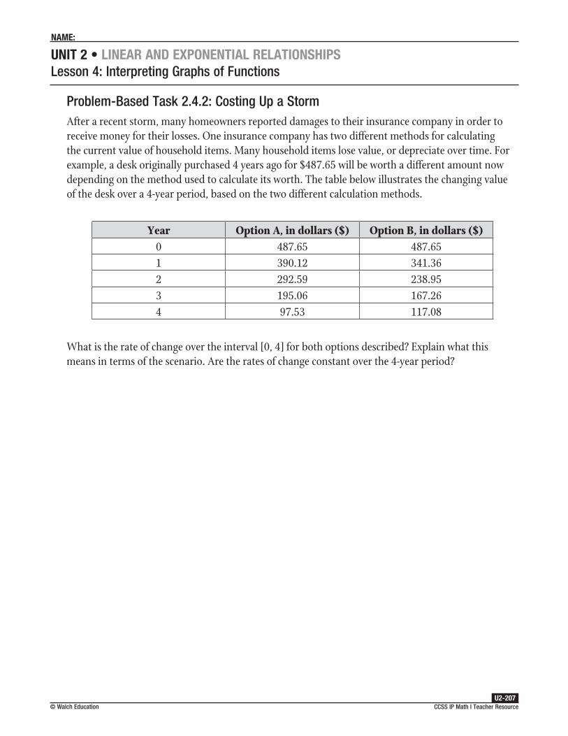
Problem-Based Task 2.4.2: Costing Up a StormAfter a recent storm, many homeowners reported damages to their insurance company in order to receive money for their losses. One insurance company has two different methods for calculating the current value of household items. Many household items lose value, or depreciate over time. For example, a desk originally purchased 4 years ago for $487.65 will be worth a different amount now depending on the method used to calculate its worth. The table below illustrates the changing value of the desk over a 4-year period, based on the two different calculation methods.

Year Option A, in dollars ($) Option B, in dollars ($)0 487.65 487.651 390.12 341.362 292.59 238.953 195.06 167.264 97.53 117.08

What is the rate of change over the interval [0, 4] for both options described? Explain what this means in terms of the scenario. Are the rates of change constant over the 4-year period?


naMe:


© Walch Education

Problem-Based Task 2.4.2: Costing Up a Storm

Coachinga. What is the interval to be observed?

b. What is the starting point of the interval for Option A?

c. What is the ending point of the interval for Option A?

d. What is the rate of change for Option A over the interval specified?

e. What does the rate of change for Option A mean in terms of this scenario?

f. What is the starting point of the interval for Option B?

g. What is the ending point of the interval for Option B?

h. What is the rate of change for Option B over the interval specified?

i. What does the rate of change for Option B mean in terms of this scenario?

j. How does the rate of change for Option A compare to the rate of change for Option B over the same interval?

k. Is the rate of change for Option A constant over the 4-year period?

l. Is the rate of change for Option B constant over the 4-year period?


Instruction


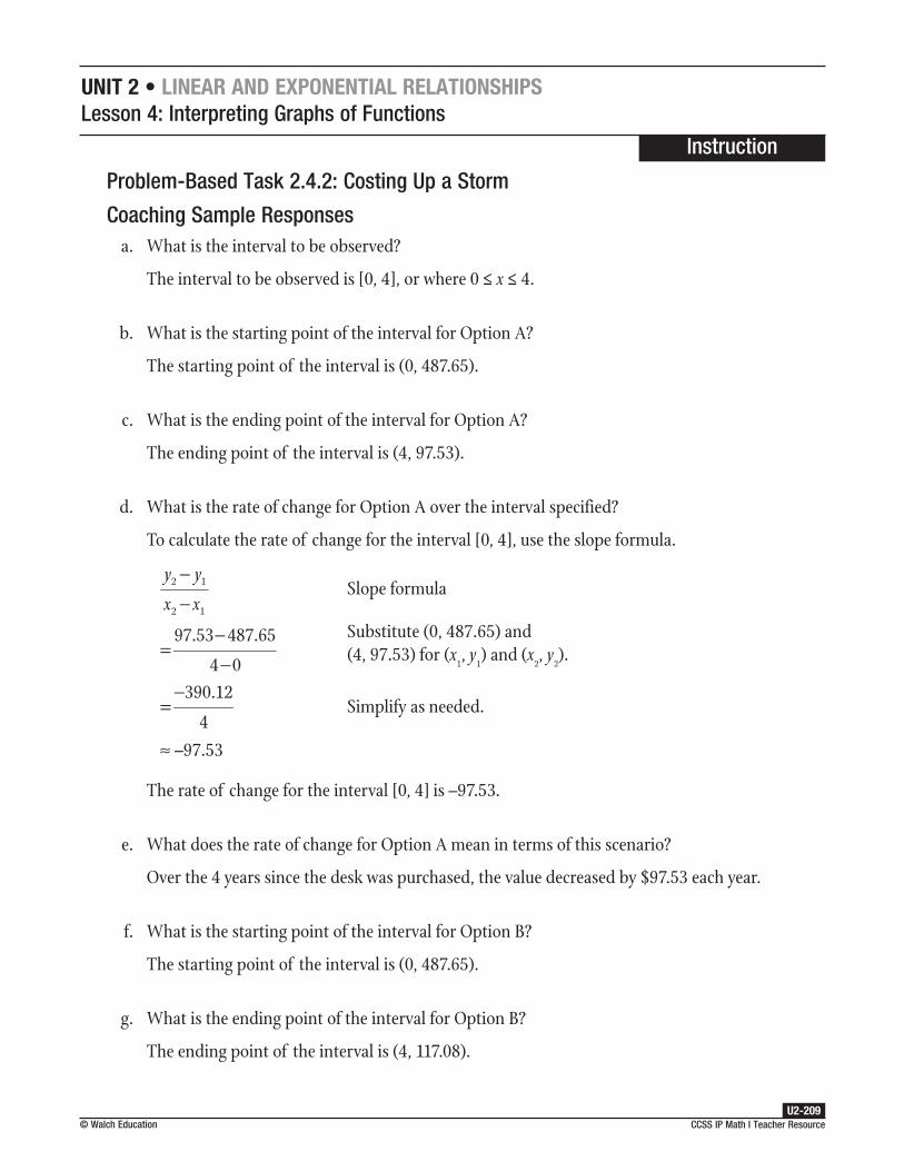
Problem-Based Task 2.4.2: Costing Up a Storm

Coaching Sample Responsesa. What is the interval to be observed?


b. What is the starting point of the interval for Option A?

The starting point of the interval is (0, 487.65).

c. What is the ending point of the interval for Option A?

The ending point of the interval is (4, 97.53).

d. What is the rate of change for Option A over the interval specified?

To calculate the rate of change for the interval [0, 4], use the slope formula.

y y

x x

−−

2 1

2 1

Slope formula

=−

−97.53 487.65

4 0


1, y

1) and (x

2, y

2).

=−390.12


≈ –97.53

The rate of change for the interval [0, 4] is –97.53.

e. What does the rate of change for Option A mean in terms of this scenario?

Over the 4 years since the desk was purchased, the value decreased by $97.53 each year.

f. What is the starting point of the interval for Option B?

The starting point of the interval is (0, 487.65).

g. What is the ending point of the interval for Option B?

The ending point of the interval is (4, 117.08).


Instruction


© Walch Education

h. What is the rate of change for Option B over the interval specified?


y y

x x

−−

2 1

2 1

Slope formula

=−−

117.08 487.65

4 0


1, y

1) and (x

2, y

2).

=−370.57


≈ –92.64

The rate of change for the interval [0, 4] is –92.64.

i. What does the rate of change for Option B mean in terms of this scenario?

Over the 4 years since the desk was purchased, the value decreased by $92.64 each year.

j. How does the rate of change for Option A compare to the rate of change for Option B over the same interval?

The rate of change over the interval [0, 4] for Option A is steeper than the rate of change for Option B. This means that the value of the desk decreases at a faster rate with Option A than with Option B.

k. Is the rate of change for Option A constant over the 4-year period?

Choose a second interval to determine if the rate is constant.

One possible interval is [1, 3].

Let (x1, y

1) = (1, 390.12) and (x

2, y

2) = (3, 195.06).

Calculate the rate of change.

y y

x x

−−

2 1

2 1

Slope formula

=−−

195.06 390.12

3 1


1, y

1) and (x

2, y

2).

=−195.06


≈ –97.53


Instruction


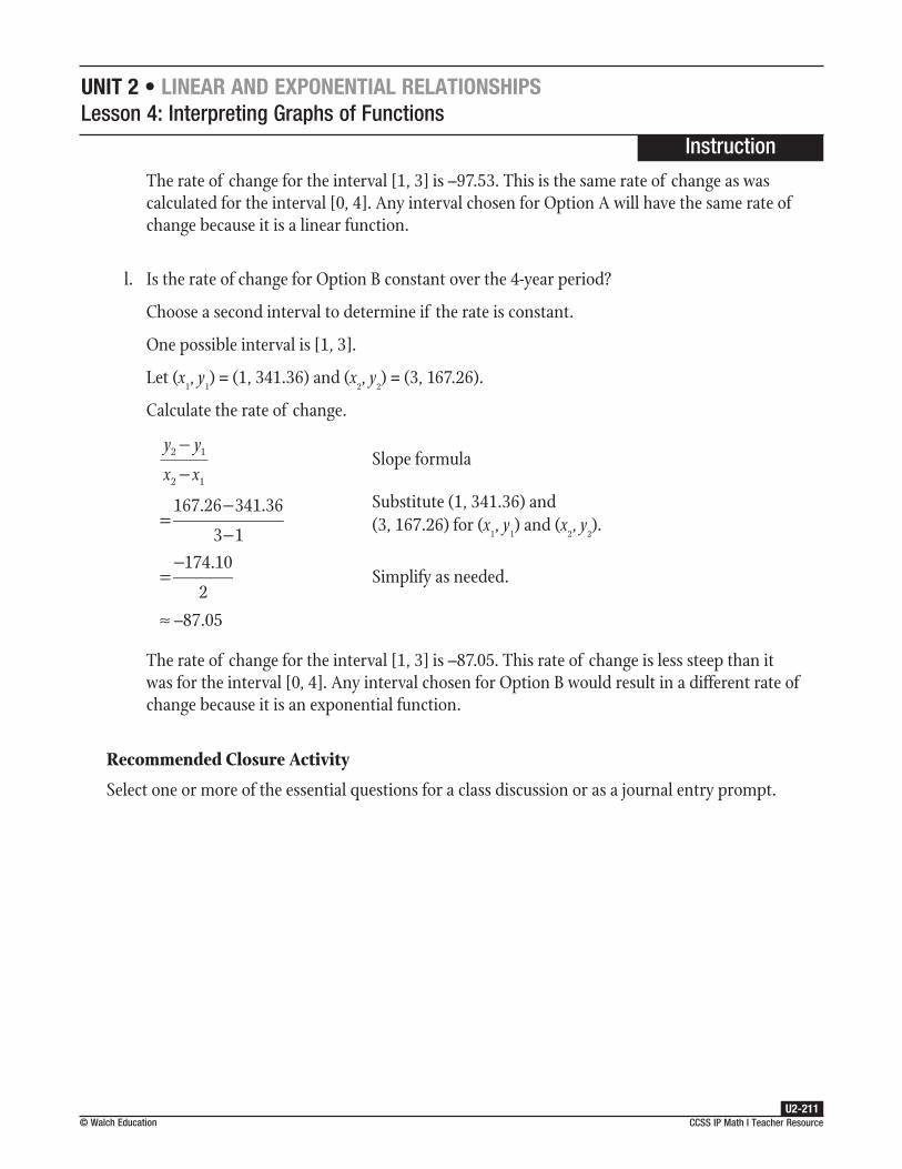
The rate of change for the interval [1, 3] is –97.53. This is the same rate of change as was calculated for the interval [0, 4]. Any interval chosen for Option A will have the same rate of change because it is a linear function.

l. Is the rate of change for Option B constant over the 4-year period?

Choose a second interval to determine if the rate is constant.

One possible interval is [1, 3].

Let (x1, y

1) = (1, 341.36) and (x

2, y

2) = (3, 167.26).

Calculate the rate of change.

y y

x x

−−

2 1

2 1

Slope formula

=−−

167.26 341.36

3 1


1, y

1) and (x

2, y

2).

=−174.10


≈ –87.05

The rate of change for the interval [1, 3] is –87.05. This rate of change is less steep than it was for the interval [0, 4]. Any interval chosen for Option B would result in a different rate of change because it is an exponential function.




naMe:


© Walch Education

Practice 2.4.2: Proving Average Rate of ChangeCalculate the rate of change for each scenario described.

1. The Beechcraft 1900D is a commuter airplane with a fuel capacity of 665 gallons. The function for this situation is f(x) = –0.9x + 665, where x represents miles flown and f(x) represents the amount of fuel remaining. What is the rate of change for this scenario?

2. The velocity of a ball thrown directly upward can be modeled by the function f(x) = –32x + 96, where x represents time in seconds and f(x) represents the height of the ball in feet. What is the rate of change for this scenario?

3. An investment of $900 is invested monthly at a rate of 4%. The function that models this

situation is f xx

= +

( ) 900 1

0.04

12

12

, where x represents time in years. What is the rate of change

for the interval [3, 10]?

4. The price of a stock started out at $150 per share and has declined to 75% of its value every

2 weeks. The function that models this decline is f xx

=( ) 150(0.75)2 , where x represents time in

weeks. What is the rate of change for the interval [1, 4]?

5. The table below lists common Celsius to Fahrenheit degree conversions. What is the rate of change for this function?

C˚ (x) F˚ (f(x))0 32

10 5020 6830 8640 104

continued


naMe:


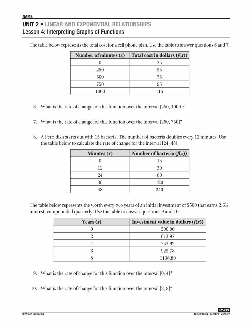
The table below represents the total cost for a cell phone plan. Use the table to answer questions 6 and 7.

Number of minutes (x) Total cost in dollars (f(x))0 35

250 55500 75750 95

1000 115

6. What is the rate of change for this function over the interval [250, 1000]?


8. A Petri dish starts out with 15 bacteria. The number of bacteria doubles every 12 minutes. Use the table below to calculate the rate of change for the interval [24, 48].

Minutes (x) Number of bacteria (f(x))0 15

12 3024 6036 12048 240

The table below represents the worth every two years of an initial investment of $500 that earns 2.6% interest, compounded quarterly. Use the table to answer questions 9 and 10.

Years (x) Investment value in dollars (f(x))0 500.002 613.974 753.926 925.788 1136.80




naMe:


© Walch Education

Lesson 2.4.3: Recognizing Average Rate of Change

Warm-Up 2.4.3The graph below shows the United States population from 1900 to 2010, as recorded by the U.S. Census Bureau.

300

325

350

275

250

225

200

175

150

125

100

75

5019001890 1910 1920 1930 1940

Census year

U.S. Population by Census

1950 1960 1970 1980 1990 2000 2010 2020

Popu

latio

n (in

mill

ions

)

1. What was the rate of change in the population from 1900 to 2000? Is this greater or less than the rate of change in the population from 2000 to 2010?

2. Which 10-year time periods have the highest and the lowest rates of change? How did you find these?

3. What do you predict the U.S. population will be in 2020? Explain your reasoning.


Instruction


Lesson 2.4.3: Recognizing Average Rate of Change Common Core State Standards



b. Recognize situations in which one quantity changes at a constant rate per unit interval relative to another.

c. Recognize situations in which a quantity grows or decays by a constant percent rate per unit interval relative to another.

Warm-Up 2.4.3 DebriefThe graph below shows the United States population from 1900 to 2010, as recorded by the U.S. Census Bureau.

300

325

350

275

250

225

200

175

150

125

100

75

5019001890 1910 1920 1930 1940

Census year

U.S. Population by Census

1950 1960 1970 1980 1990 2000 2010 2020

Popu

latio

n (in

mill

ions

)

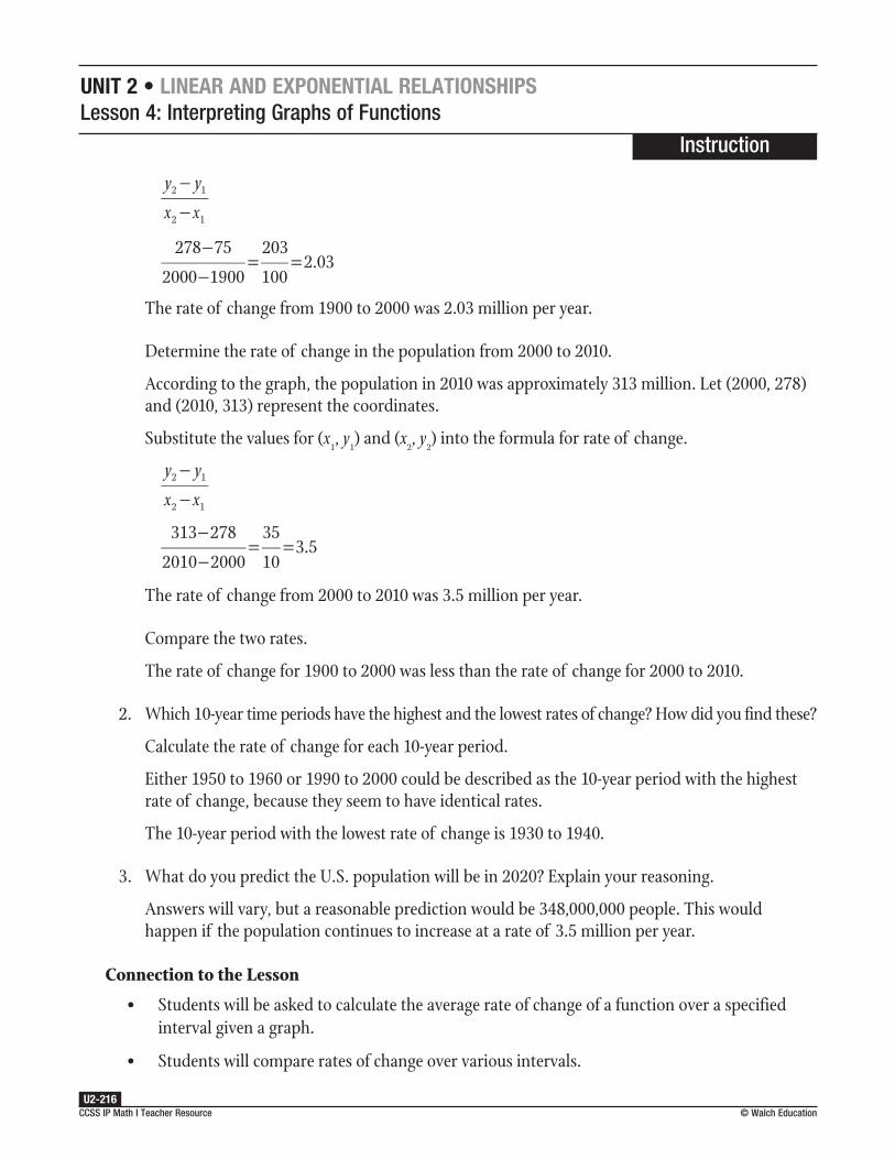
1. What was the rate of change in the population from 1900 to 2000? Is this greater or less than the rate of change in the population from 2000 to 2010?

The rate of change in the population from 1900 to 2000 can be found using the rate of change

formula, y y

x x

−−

2 1

2 1

.

Determine the population for the years 1900 and 2000.

According to the graph, the population in 1900 was 75 million and the population in 2000 was approximately 278 million. Let (1900, 75) and (2000, 278) represent the coordinates.

Substitute the values for (x1, y

1) and (x

2, y

2) into the formula for rate of change.


Instruction


© Walch Education

y y

x x

−−

2 1

2 1

−−

= =278 75

2000 1900

203

1002.03

The rate of change from 1900 to 2000 was 2.03 million per year.

Determine the rate of change in the population from 2000 to 2010.

According to the graph, the population in 2010 was approximately 313 million. Let (2000, 278) and (2010, 313) represent the coordinates.

Substitute the values for (x1, y

1) and (x

2, y

2) into the formula for rate of change.

y y

x x

−−

2 1

2 1

−−

= =313 278

2010 2000

35

103.5

The rate of change from 2000 to 2010 was 3.5 million per year.

Compare the two rates.

The rate of change for 1900 to 2000 was less than the rate of change for 2000 to 2010.

2. Which 10-year time periods have the highest and the lowest rates of change? How did you find these?

Calculate the rate of change for each 10-year period.

Either 1950 to 1960 or 1990 to 2000 could be described as the 10-year period with the highest rate of change, because they seem to have identical rates.

The 10-year period with the lowest rate of change is 1930 to 1940.

3. What do you predict the U.S. population will be in 2020? Explain your reasoning.

Answers will vary, but a reasonable prediction would be 348,000,000 people. This would happen if the population continues to increase at a rate of 3.5 million per year.


• Students will be asked to calculate the average rate of change of a function over a specified interval given a graph.

• Students will compare rates of change over various intervals.


Instruction


Prerequisite Skills


• reading points from a graph

• applying the order of operations

• interpreting interval notation

IntroductionPreviously, we calculated the rate of change of linear functions as well as intervals of exponential functions. We observed that the rate of change of exponential functions changed if we focused on different intervals of the function. Here, we will focus on graphs of linear and exponential functions and learn how to estimate the rates of change.

Key Concepts

• To determine the rate of change of a function, first identify the coordinates of the interval being observed.

• Sometimes it is necessary to estimate the values for y.

• The resulting calculation may be an estimation of the rate of change for the interval identified for the given function.

Estimating Rate of Change from a Graph


2. Identify (x1, y

1) as the starting point of the interval.

3. Identify (x2, y

2) as the ending point of the interval.


1) and (x

2, y

2) into the slope formula to calculate the rate of change.

5. The result is the estimated rate of change for the interval between the two points identified.


• incorrectly choosing the values of the indicated interval to estimate the rate of change

• incorrectly estimating the values for the indicated interval

• substituting incorrect values into the formula for calculating rate of change


Instruction


© Walch Education


The graph below compares the distance a small motor scooter can travel in miles to the amount of fuel used in gallons. What is the rate of change for this scenario?

0 10 20 30 40 50 60 70 80 90 100 110 120 130 140 1500.1

0.2

0.3

0.4

0.5

0.6

0.7

0.8

0.9

1

1.1

1.2

1.3

1.4

1.5

1.6

1.7

1.8

1.9

2

Distance in miles

Fuel

rem

aini

ng in

tank

(gal

lons

)


The function is linear, so the rate of change will be constant for any interval of the function.


Instruction


2. Choose a starting point of the interval.

Choose a point on the graph with coordinates that are easy to estimate.

It appears as though the line crosses the y-axis at the point (0, 1.5).

Let (0, 1.5) be the starting point of the interval.

3. Choose an ending point of the interval.

Choose another point on the graph with coordinates that are easy to estimate.

It appears as though the line crosses the x-axis at the point (155, 0).

Let (155, 0) be the ending point of the interval.

4. Substitute (0, 1.5) and (155, 0) into the slope formula to calculate the rate of change.

y y

x x

−−

2 1

2 1

Slope formula

=−

−0 1.5

155 0

Substitute (0, 1.5) and (155, 0) for (x

1, y

1) and (x

2, y

2).

=−1.5155

Simplify as needed.

≈ –0.01

The rate of change for this function is approximately –0.01 gallons per mile. The amount of fuel decreases by 0.01 gallons per mile.


Instruction


© Walch Education

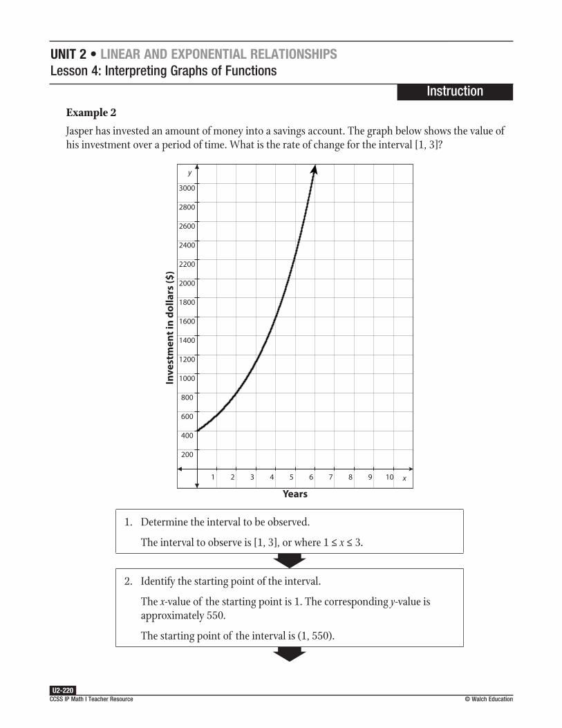
Example 2

Jasper has invested an amount of money into a savings account. The graph below shows the value of his investment over a period of time. What is the rate of change for the interval [1, 3]?

1 2 3 4 5 6 7 8 9 10

200

400

600

800

1000

1200

1400

1600

1800

2000

2200

2400

2600

2800

3000

Years

Inve

stm

ent i

n do

llars

($)


The interval to observe is [1, 3], or where 1 ≤ x ≤ 3.

2. Identify the starting point of the interval.

The x-value of the starting point is 1. The corresponding y-value is approximately 550.

The starting point of the interval is (1, 550).


Instruction


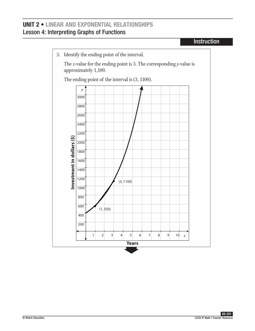
3. Identify the ending point of the interval.

The x-value for the ending point is 3. The corresponding y-value is approximately 1,100.

The ending point of the interval is (3, 1100).

1 2 3 4 5 6 7 8 9 10

200

400

600

800

1000

1200

1400

1600

1800

2000

2200

2400

2600

2800

3000

Years

Inve

stm

ent i

n do

llars

($)

(1, 550)

(3, 1100)


Instruction


© Walch Education

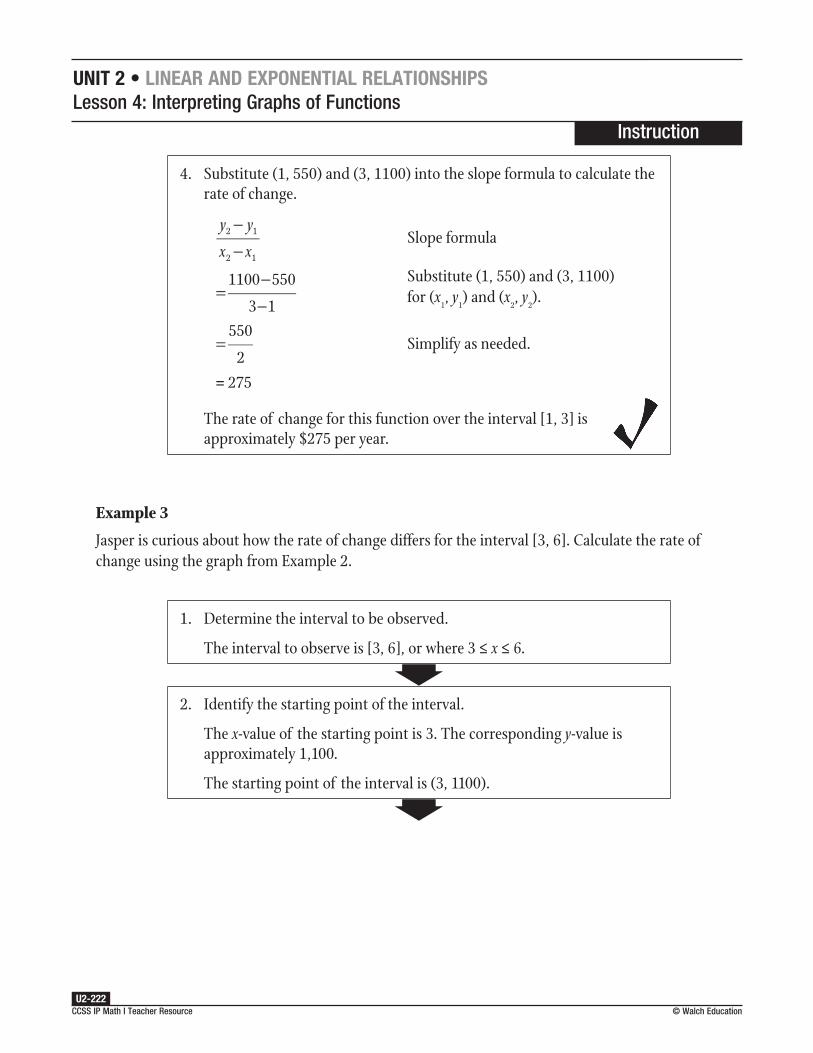
4. Substitute (1, 550) and (3, 1100) into the slope formula to calculate the rate of change.

y y

x x

−−

2 1

2 1

Slope formula

=−

−1100 550

3 1


1, y

1) and (x

2, y

2).

=550


= 275

The rate of change for this function over the interval [1, 3] is approximately $275 per year.

Example 3

Jasper is curious about how the rate of change differs for the interval [3, 6]. Calculate the rate of change using the graph from Example 2.


The interval to observe is [3, 6], or where 3 ≤ x ≤ 6.

2. Identify the starting point of the interval.

The x-value of the starting point is 3. The corresponding y-value is approximately 1,100.

The starting point of the interval is (3, 1100).


Instruction


3. Identify the ending point of the interval.

The x-value for the ending point is 6. The corresponding y-value is approximately 3,100.

The ending point of the interval is (6, 3100).

1 2 3 4 5 6 7 8 9 10

200

400

600

800

1000

1200

1400

1600

1800

2000

2200

2400

2600

2800

3000

Years

Inve

stm

ent i

n do

llars

($)

(1, 550)

(3, 1100)

(6, 3100)


Instruction


© Walch Education

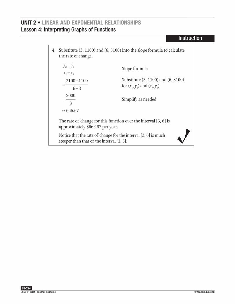
4. Substitute (3, 1100) and (6, 3100) into the slope formula to calculate the rate of change.

y y

x x

−−

2 1

2 1

Slope formula

=−−

3100 1100

6 3


1, y

1) and (x

2, y

2).

=2000


≈ 666.67

The rate of change for this function over the interval [3, 6] is approximately $666.67 per year.

Notice that the rate of change for the interval [3, 6] is much steeper than that of the interval [1, 3].


naMe:


Problem-Based Task 2.4.3: Dwindling ConcentrationsThe liver and kidneys work to eliminate medications from the body exponentially. It is important for doctors to understand how much of any medication remains in the body after a certain period of time in order to prescribe the correct dosage. The graph below shows the amount in milligrams of a certain medication remaining in the body each hour after one dose.

0 1 2 3 4 5 6 7 8 9 10

50

100

150

200

250

300

350

400

450

500

550

600

650

700

750

Time (hours)

Am

ount

of m

edic

atio

n re

mai

ning

(mg)

What is the rate of change for the interval [1, 3]? How does this rate of change compare to the rate of change for the interval [3, 10]?

It is not uncommon for more than one dose of medication to be prescribed. Based on your findings, why would a patient be instructed to take a second dose of medication 12 hours after the initial dose?


naMe:


© Walch Education

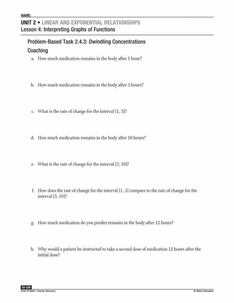
Problem-Based Task 2.4.3: Dwindling Concentrations

Coachinga. How much medication remains in the body after 1 hour?

b. How much medication remains in the body after 3 hours?

c. What is the rate of change for the interval [1, 3]?

d. How much medication remains in the body after 10 hours?

e. What is the rate of change for the interval [3, 10]?

f. How does the rate of change for the interval [1, 3] compare to the rate of change for the interval [3, 10]?

g. How much medication do you predict remains in the body after 12 hours?

h. Why would a patient be instructed to take a second dose of medication 12 hours after the initial dose?


Instruction


Problem-Based Task 2.4.3: Dwindling Concentrations

Coaching Sample Responsesa. How much medication remains in the body after 1 hour?

After 1 hour, approximately 450 milligrams of medication remain in the body.

b. How much medication remains in the body after 3 hours?

After 3 hours, approximately 160 milligrams of medication remain.

c. What is the rate of change for the interval [1, 3?]


y y

x x

−−

2 1

2 1

Slope formula

=−−

160 450

3 1


1, y

1) and (x

2, y

2).

=−2902

Simplify as needed.

= –145

The rate of change for the interval [1, 3] is approximately –145 milligrams per hour.

d. How much medication remains in the body after 10 hours?

After 10 hours, approximately 5 milligrams of medication remain.

e. What is the rate of change for the interval [3, 10]?


y y

x x

−−

2 1

2 1

Slope formula

=−

−5 160

10 3


1, y

1) and (x

2, y

2).

=−1557

Simplify as needed.

≈ –22

The rate of change for the interval [3, 10] is approximately –22 milligrams per hour.


Instruction


© Walch Education

f. How does the rate of change for the interval [1, 3] compare to the rate of change for the interval [3, 10]?

The rate of change for the interval [1, 3] is steeper than the rate of change for the interval [3, 10]. Medication is eliminated from the body at a much faster rate within the first 3 hours of the initial dose than over the next 7 hours.

g. How much medication do you predict remains in the body after 12 hours?

The amount of medication in the body 12 hours after the initial dose is very close to 0 milligrams.

h. Why would a patient be instructed to take a second dose of medication 12 hours after the initial dose?

There is virtually no medication left 12 hours after the initial dose. In order for this particular medication to be effective, more medication would need to enter the body.




naMe:


Practice 2.4.3: Recognizing Average Rate of ChangeThe graph below shows the amount of paint needed to paint the trim molding of a house. Use the graph to answer questions 1 and 2.

100 200 300 400 500 600 700 800 900 1000 1100 1200 1300 1400

0.2

0.4

0.6

0.8

1

1.2

1.4

1.6

1.8

2

Length of trim (feet)

Am

ount

of p

aint

(ga

llons

)

1. What is the approximate rate of change for the interval [150, 500]?


continued


naMe:


© Walch Education

The graph below shows the value of the U.S. dollar compared to the value of the Euro on a specific day. Use the graph to answer questions 3–5.

5 10 15 20 25 30 35 40 45 50 55 60 65 70 75 80 85 90 95 100

5

10

15

20

25

30

35

40

45

50

55

60

65

70

75

80

Value of U.S. dollar

Valu

e of

Eur

o



5. Could you predict the rate of change for a third interval on the same graph? If so, what is your prediction?

continued


naMe:


Each year, employees at a wildlife park record the total number of visitors to the park over Labor Day weekend. The graph below shows the number of visitors for each of the last 10 years. Use the graph to answer questions 6 and 7.

1 2 3 4 5 6 7 8 9 10

100

200

300

400

500

600

700

800

Year

Tota

l num

ber o

f vis

itor

s



continued


naMe:


© Walch Education

The graph below shows the yearly population of a small town. Use the graph to answer questions 8–10.

1 2 3 4 5 6 7 8 9 10 11 12 13 14 15 16 17 18 19 20

1000

2000

3000

4000

5000

6000

7000

8000

9000

Years

Popu

lati

on



10. How does the rate of change differ for each interval?

Documents

naMe: Unit 2 • Linear and exponentiaL reLationships …windrivermath.wikispaces.com/.../view/M1+Unit+2+Lesson+4.pdfLesson 2.4.1: Identifying Key Features of Linear and Exponential