Naïve Bayes - filebox.ece.vt.edujbhuang/teaching/ECE5424-CS5824/sp19/slides/Lec04.pdf · •Naive Bayes. Random variables •Outcome space S •Space of possible outcomes •Random

Naïve Bayes

Jia-Bin Huang

Virginia Tech Spring 2019ECE-5424G / CS-5824

Administrative

• HW 1 out today. Please start early!

• Office hours• Chen: Wed 4pm-5pm

• Shih-Yang: Fri 3pm-4pm

• Location: Whittemore 266

Linear Regression

• Model representationℎ𝜃 𝑥 = 𝜃0 + 𝜃1𝑥1 + 𝜃2𝑥2 +⋯+ 𝜃𝑛𝑥𝑛 = 𝜃⊤𝑥

• Cost function 𝐽 𝜃 =1

2𝑚σ𝑖=1𝑚 ℎ𝜃 𝑥 𝑖 − 𝑦 𝑖 2

• Gradient descent for linear regressionRepeat until convergence {𝜃𝑗 ≔ 𝜃𝑗 − 𝛼

1

𝑚σ𝑖=1𝑚 ℎ𝜃 𝑥 𝑖 − 𝑦 𝑖 𝑥𝑗

𝑖}

• Features and polynomial regression

Can combine features; can use different functions to generate features (e.g., polynomial)

• Normal equation 𝜃 = (𝑋⊤𝑋)−1𝑋⊤𝑦

(𝑥0) Size in feet^2(𝑥1)

Number of bedrooms

(𝑥2)

Number of floors (𝑥3)

Age of home (years) (𝑥4)

Price ($) in 1000’s (y)

1 2104 5 1 45 460

1 1416 3 2 40 232

1 1534 3 2 30 315

1 852 2 1 36 178

… …

𝑦 =

460232315178

𝜃 = (𝑋⊤𝑋)−1𝑋⊤𝑦Slide credit: Andrew Ng

Least square solution

• 𝐽 𝜃 =1


=1

2𝑚σ𝑖=1𝑚 𝜃⊤𝑥(𝑖) − 𝑦 𝑖 2

=1

2𝑚𝑋𝜃 − 𝑦 2

2

•𝜕

𝜕𝜃𝐽 𝜃 = 0

• 𝜃 = (𝑋⊤𝑋)−1𝑋⊤𝑦

Justification/interpretation 1

•Geometric interpretation

𝑿 =

1 ← 𝒙(1) →1⋮1

← 𝒙(2) →⋮

← 𝒙(𝑚) →

=↑𝒛𝟎

↑𝒛𝟏

↑𝒛𝟐

⋯↑𝒛𝒏

↓ ↓ ↓ ↓

• 𝑿𝜽: column space of 𝑿 or span({𝒛𝟎, 𝒛𝟏, ⋯ , 𝒛𝒏})

• Residual 𝑿𝜽 − 𝐲 is orthogonal to the column space of 𝑿

• 𝑿⊤ 𝑿𝜽 − 𝐲 = 0 → (𝑿⊤𝑿)𝜽 = 𝑿⊤𝒚

𝒚

column space of 𝑿

𝑿𝜽

𝑿𝜽 − 𝒚


•Probabilistic model• Assume linear model with Gaussian errors

𝑝𝜃 𝑦 𝑖 𝑥 𝑖 =1

2𝜋𝜎2exp(−

1

2𝜎2(𝑦 𝑖 − 𝜃⊤𝑥 𝑖 )

• Solving maximum likelihood

argmin𝜃

ෑ

𝑖=1

𝑚

𝑝𝜃 𝑦 𝑖 𝑥 𝑖

argmin𝜃

log(ෑ

𝑖=1

𝑚

𝑝 𝑦 𝑖 𝑥 𝑖 ) = argmin𝜃

1

2𝜎2

𝑖=1

𝑚1

2𝜃⊤𝑥 𝑖 − 𝑦 𝑖 2

Image credit: CS 446@UIUC


• Loss minimization

𝐽 𝜃 =1

2𝑚

𝑖=1

𝑚

ℎ𝜃 𝑥 𝑖 − 𝑦 𝑖 2=

1

𝑚

𝑖=1

𝑚

𝐿𝑙𝑠 ℎ𝜃 𝑥 𝑖 , 𝑦 𝑖

• 𝐿𝑙𝑠 𝑦, ො𝑦 =1

2𝑦 − ො𝑦 2

2: Least squares loss

• Empirical Risk Minimization (ERM)1

𝑚

𝑖=1

𝑚

𝐿𝑙𝑠 𝑦 𝑖 , ො𝑦

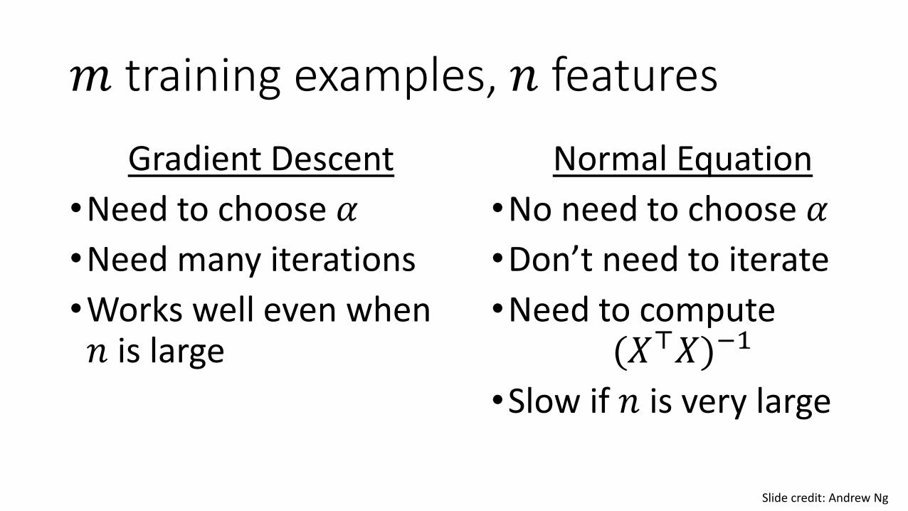
𝑚 training examples, 𝑛 features

Gradient Descent

•Need to choose 𝛼

•Need many iterations

•Works well even when 𝑛 is large

Normal Equation

•No need to choose 𝛼

•Don’t need to iterate

•Need to compute (𝑋⊤𝑋)−1

•Slow if 𝑛 is very large

Slide credit: Andrew Ng

Things to remember

• Model representationℎ𝜃 𝑥 = 𝜃0 + 𝜃1𝑥1 + 𝜃2𝑥2 +⋯+ 𝜃𝑛𝑥𝑛 = 𝜃⊤𝑥

• Cost function 𝐽 𝜃 =1


• Gradient descent for linear regressionRepeat until convergence {𝜃𝑗 ≔ 𝜃𝑗 − 𝛼

1

𝑚σ𝑖=1𝑚 ℎ𝜃 𝑥 𝑖 − 𝑦 𝑖 𝑥𝑗

𝑖}

• Features and polynomial regression

Can combine features; can use different functions to generate features (e.g., polynomial)

• Normal equation 𝜃 = (𝑋⊤𝑋)−1𝑋⊤𝑦

Today’s plan

•Probability basics

• Estimating parameters from data• Maximum likelihood (ML)

• Maximum a posteriori estimation (MAP)

•Naïve Bayes

Today’s plan




•Naive Bayes

Random variables

• Outcome space S• Space of possible outcomes

• Random variables• Functions that map outcomes to real numbers

• Event E• Subset of S

Visualizing probability 𝑃(𝐴)

A is true

Sample space

Area = 1

A is false

𝑃 𝐴 = Area of the blue circle

Visualizing probability 𝑃 𝐴 + P ~A

A is true

A is false

𝑃 𝐴 + P ~A = 1

Visualizing probability 𝑃 𝐴

A^~B

𝑃 𝐴 = P(A, B) + P A,~𝐵

B

A^B

Visualizing conditional probability

A

𝑃 𝐴|𝐵 = 𝑃 𝐴, 𝐵 /𝑃(𝐵)

B

A^B

Corollary: The chain rule

𝑃 𝐴, 𝐵 = 𝑃 𝐴|𝐵 𝑃(𝐵)

Bayes rule

A𝑃 𝐴|𝐵 =

𝑃 𝐴, 𝐵

𝑃 𝐵

=𝑃 𝐵 𝐴 𝑃 𝐴

𝑃(𝐵)

B

A^B

Corollary: The chain rule

𝑃 𝐴, 𝐵 = 𝑃 𝐴|𝐵 𝑃 𝐵 = P B P A B

Thomas Bayes

Other forms of Bayes rule

𝑃 𝐴|𝐵 =𝑃 𝐵 𝐴 𝑃 𝐴

𝑃(𝐵)

𝑃 𝐴|𝐵, 𝑋 =𝑃 𝐵 𝐴, 𝑋 𝑃 𝐴, 𝑋

𝑃(𝐵, 𝑋)


𝑃 𝐵 𝐴 𝑃 𝐴 + 𝑃 𝐵 ~𝐴 𝑃(~𝐴)

Applying Bayes rule


𝑃 𝐵 𝐴 𝑃 𝐴 + 𝑃 𝐵 ~𝐴 𝑃(~𝐴)

• A = you have the flu B = you just coughed

• Assume:• 𝑃 𝐴 = 0.05• 𝑃 𝐵 𝐴 = 0.8• 𝑃 𝐵 ~𝐴 = 0.2

• What is P(flu | cough) = P(A|B)?

𝑃 𝐴|𝐵 =0.8 × 0.05

0.8 × 0.05 + 0.2 × 0.95~0.17

Slide credit: Tom Mitchell

Why we are learning this?

Learn 𝑃 𝑌|𝑋

ℎ𝑥 𝑦

Hypothesis

Joint distribution

• Making a joint distribution of M variables

1. Make a truth table listing all combinations

2. For each combination of values, say how probable it is

3. Probability must sum to 1

A B C Prob

0 0 0 0.30

0 0 1 0.05

0 1 0 0.10

0 1 1 0.05

1 0 0 0.05

1 0 1 0.10

1 1 0 0.25

1 1 1 0.10


Using joint distribution

• Can ask for any logical expression involving these variables

• 𝑃 𝐸 = σrowsmatching E𝑃(row)

• 𝑃 𝐸1|𝐸2 =σrowsmatching E1 and 𝐸2

𝑃 row

σrowsmatching 𝐸2𝑃 row


The solution to learn 𝑃 𝑌|𝑋 ?

• Main problem: learning 𝑃 𝑌|𝑋 may require more data than we have

• Say, learning a joint distribution with 100 attributes

• # of rows in this table?

• # of people on earth?

2100 ≥ 1030

109


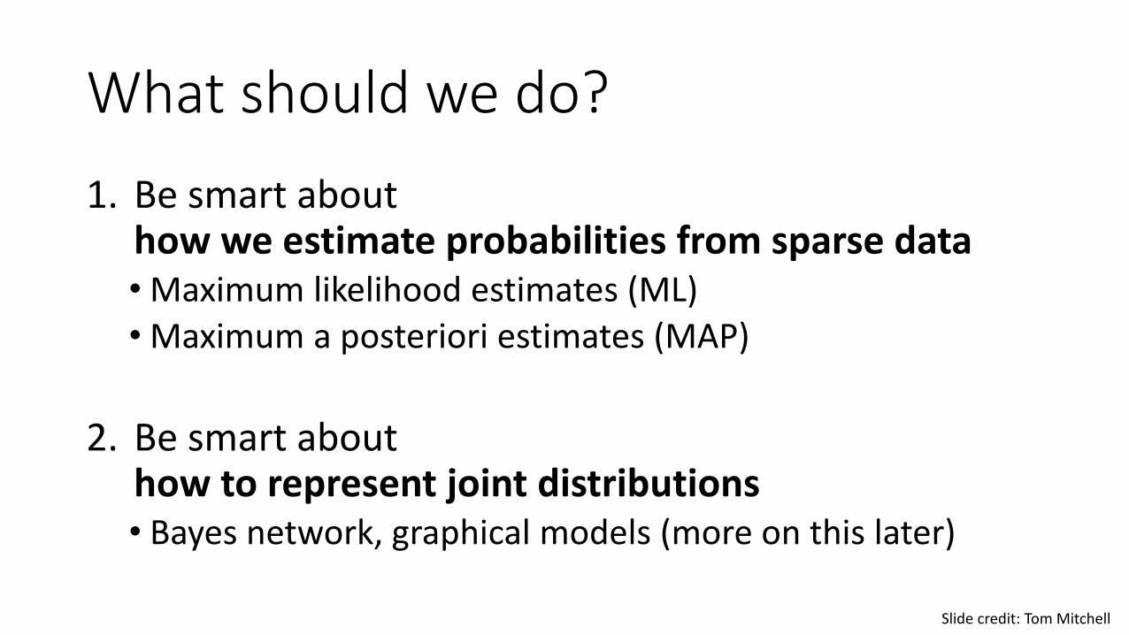
What should we do?

1. Be smart about how we estimate probabilities from sparse data• Maximum likelihood estimates (ML)• Maximum a posteriori estimates (MAP)

2. Be smart about how to represent joint distributions• Bayes network, graphical models (more on this later)


Today’s plan



• Maximum a posteriori (MAP)

•Naive Bayes

Estimating the probability

• Flip the coin repeatedly, observing• It turns heads 𝛼1 times

• It turns tails 𝛼0 times

• Your estimate for 𝑃 𝑋 = 1 is?

• Case A: 100 flips: 51 Heads (𝑋 = 1), 49 Tails (𝑋 = 0)

𝑃 𝑋 = 1 = ?

• Case B: 3 flips: 2 Heads (𝑋 = 1), 1 Tails (𝑋 = 0)

𝑃 𝑋 = 1 = ?

𝑋 = 1 𝑋 =0


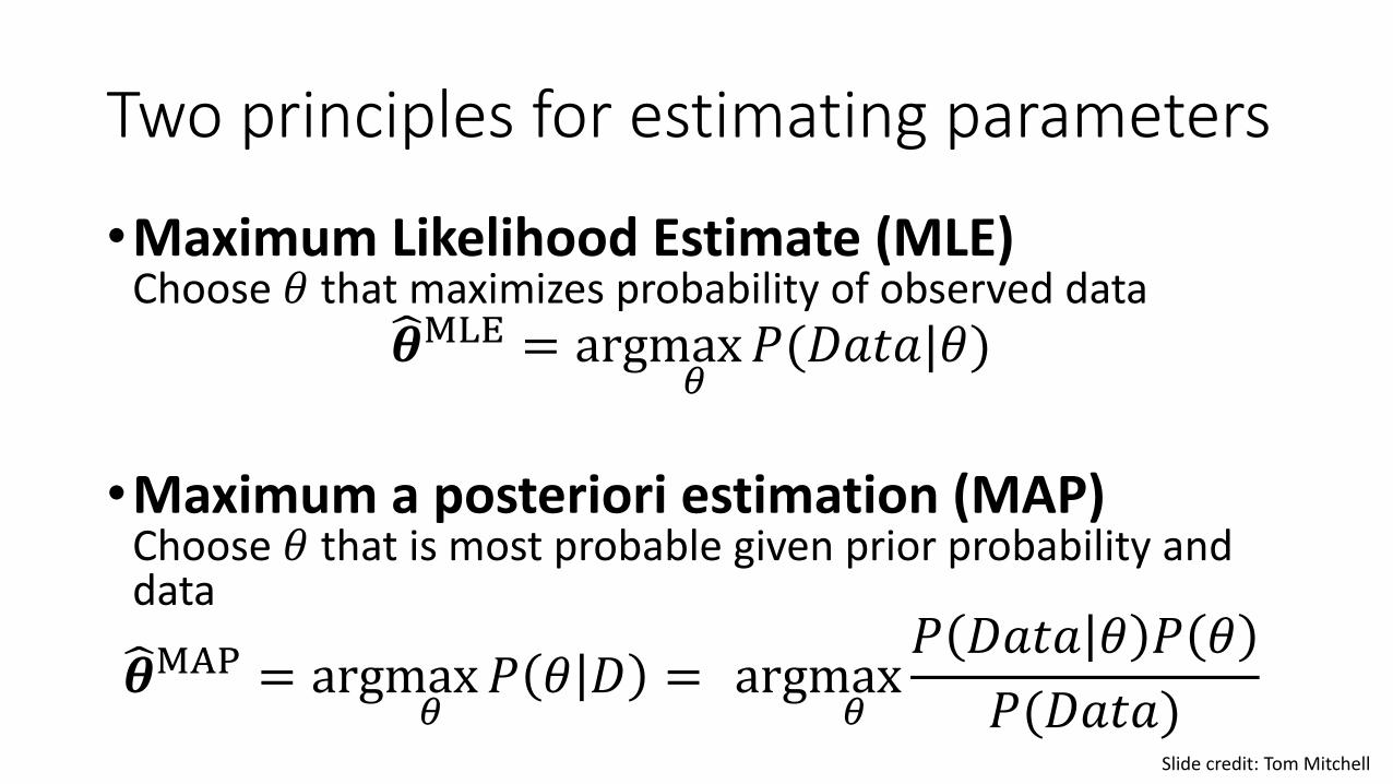
Two principles for estimating parameters

•Maximum Likelihood Estimate (MLE) Choose 𝜃 that maximizes probability of observed data

𝜽MLE = argmax𝜃

𝑃(𝐷𝑎𝑡𝑎|𝜃)

•Maximum a posteriori estimation (MAP)Choose 𝜃 that is most probable given prior probability and data

𝜽MAP = argmax𝜃

𝑃 𝜃 𝐷 = argmax𝜃

𝑃 𝐷𝑎𝑡𝑎 𝜃 𝑃 𝜃

𝑃(𝐷𝑎𝑡𝑎)Slide credit: Tom Mitchell

Two principles for estimating parameters

•Maximum Likelihood Estimate (MLE) Choose 𝜃 that maximizes 𝑃 𝐷𝑎𝑡𝑎 𝜃

𝜽MLE =𝛼1

𝛼1 + 𝛼0

•Maximum a posteriori estimation (MAP)Choose 𝜃 that maximize 𝑃 𝜃 𝐷𝑎𝑡𝑎

𝜽MAP =(𝛼1 + #halluciated 1s)

(𝛼1+#halluciated 1𝑠) + (𝛼0 + #halluciated 0s)Slide credit: Tom Mitchell

Maximum likelihood estimate

• Each flip yields Boolean value for 𝑋

𝑋 ∼ Bernoulli: 𝑃 𝑋 = 𝜃𝑋 1 − 𝜃 1−𝑋

• Data set 𝐷 of independent, identically distributed (iid) flips, produces 𝛼1 ones, 𝛼0 zeros

𝑃 𝐷 𝜃 = 𝑃 𝛼1, 𝛼0 𝜃 = 𝜃𝛼1 1 − 𝜃 𝛼0

𝜽 = argmax𝜃

𝑃(𝐷|𝜃) =𝛼1

𝛼1 + 𝛼0

𝑋 = 1 𝑋 =0

𝑃 𝑋 = 1 = 𝜃𝑃 𝑋 = 0 = 1 − 𝜃


Beta prior distribution 𝑃 𝜃

•𝑃 𝜃 = 𝐵𝑒𝑡𝑎 𝛽1, 𝛽0 =1

𝐵(𝛽1,𝛽0)𝜃𝛽1−1 1 − 𝜃 𝛽0−1


Maximum likelihood estimate

• Data set 𝐷 of iid flips, produces 𝛼1 ones, 𝛼0 zeros

𝑃 𝐷 𝜃 = 𝑃 𝛼1, 𝛼0 𝜃 = 𝜃𝛼1 1 − 𝜃 𝛼0

• Assume prior (Conjugate prior: Closed form representation of posterior)

𝑃 𝜃 = 𝐵𝑒𝑡𝑎 𝛽1, 𝛽0 =1

𝐵(𝛽1, 𝛽0)𝜃𝛽1−1 1 − 𝜃 𝛽0−1

𝜽 = argmax𝜃

𝑃 𝐷 𝜃 P(𝜃) =𝛼1 + 𝛽1 − 1

(𝛼1 + 𝛽1 − 1) + (𝛼0 + 𝛽0 − 1)

𝑋 = 1 𝑋 =0


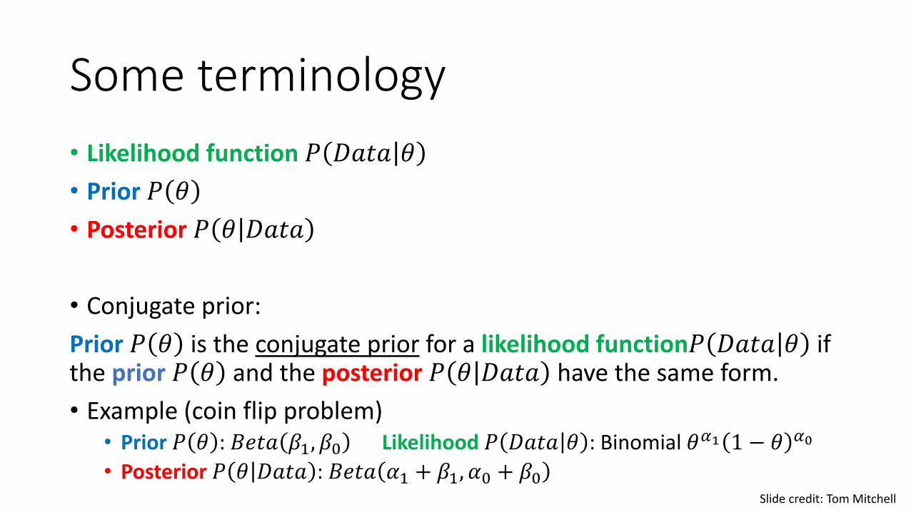
Some terminology

• Likelihood function 𝑃 𝐷𝑎𝑡𝑎 𝜃

• Prior 𝑃 𝜃

• Posterior 𝑃 𝜃 𝐷𝑎𝑡𝑎

• Conjugate prior:

Prior 𝑃 𝜃 is the conjugate prior for a likelihood function𝑃 𝐷𝑎𝑡𝑎 𝜃 if the prior 𝑃 𝜃 and the posterior 𝑃 𝜃 𝐷𝑎𝑡𝑎 have the same form.

• Example (coin flip problem)• Prior 𝑃 𝜃 : 𝐵𝑒𝑡𝑎 𝛽1, 𝛽0 Likelihood 𝑃 𝐷𝑎𝑡𝑎 𝜃 : Binomial 𝜃𝛼1 1 − 𝜃 𝛼0

• Posterior 𝑃 𝜃 𝐷𝑎𝑡𝑎 : 𝐵𝑒𝑡𝑎 𝛼1 + 𝛽1, 𝛼0 + 𝛽0Slide credit: Tom Mitchell

How many parameters?

• Suppose 𝑋 = [𝑋1, ⋯ , 𝑋𝑛], where

𝑋𝑖 and 𝑌 are Boolean random variables

To estimate 𝑃 𝑌 𝑋1, ⋯ , 𝑋𝑛)

When 𝑛 = 2 (Gender, Hours-worked)?

When 𝑛 = 30?


Can we reduce paras using Bayes rule?

𝑃 𝑌|𝑋 =𝑃 𝑋 𝑌 𝑃 𝑌

𝑃(𝑋)

•How many parameters for 𝑃(𝑋1, ⋯ , 𝑋𝑛|𝑌)?2𝑛 − 1 × 2

•How many parameters for 𝑃 𝑌 ?1


Today’s plan




•Naive Bayes

Naïve Bayes

• Assumption:

𝑃 𝑋1, ⋯ , 𝑋𝑛 𝑌 = ෑ

𝑗=1

𝑛

𝑃(𝑋𝑗|𝑌)

• i.e., 𝑋𝑖 and 𝑋𝑗 are conditionally independentgiven 𝑌 for 𝑖 ≠ 𝑗


Conditional independence

• Definition: 𝑋 is conditionally independent of 𝑌 given 𝑍, if the probability distribution governing 𝑋 is independent of the value of 𝑌, given the value of 𝑍

∀𝑖, 𝑗, 𝑘 𝑃 𝑋 = 𝑥𝑖 𝑌 = 𝑦𝑗 , 𝑍 = 𝑧𝑘) = 𝑃(𝑋 = 𝑥𝑖|𝑍𝑘)

𝑃 𝑋 𝑌, 𝑍 = 𝑃(𝑋|𝑍)

Example:𝑃 Thunder Rain, Lightning = 𝑃(Thunder|Lightning)


Applying conditional independence

• Naïve Bayes assumes 𝑋𝑖 are conditionally independent given 𝑌

e.g., 𝑃 𝑋1 𝑋2, 𝑌 = 𝑃(𝑋1|𝑌)

𝑃 𝑋1, 𝑋2 𝑌 = 𝑃 𝑋1 𝑋2, 𝑌 𝑃 𝑋2 𝑌

= 𝑃 𝑋1 𝑌 𝑃(𝑋2|𝑌)

General form: 𝑃 𝑋1, ⋯ , 𝑋𝑛 𝑌 = ς𝑗=1𝑛 𝑃(𝑋𝑗|𝑌)

How many parameters to describe 𝑃 𝑋1, ⋯ , 𝑋𝑛 𝑌 ? 𝑃(Y)?

• Without conditional indep assumption?

• With conditional indep assumption?Slide credit: Tom Mitchell

Naïve Bayes classifier

• Bayes rule:

𝑃 𝑌 = 𝑦𝑘 𝑋1, ⋯ , 𝑋𝑛) =𝑃(𝑌 = 𝑦𝑘)𝑃(𝑋1, ⋯ , 𝑋𝑛 𝑌 = 𝑦𝑘

σ𝑗 𝑃 𝑌 = 𝑦𝑗 𝑃 𝑋1, ⋯ , 𝑋𝑛 𝑌 = 𝑦𝑗

• Assume conditional independence among 𝑋𝑖’s:

𝑃 𝑌 = 𝑦𝑘 𝑋1, ⋯ , 𝑋𝑛) =𝑃 𝑌 = 𝑦𝑘 Π𝑖𝑃 𝑋𝑖 𝑌 = 𝑦𝑘)

σ𝑗 𝑃 𝑌 = 𝑦𝑗 Π𝑖𝑃 𝑋𝑖 𝑌 = 𝑦𝑗)

• Pick the most probable Y𝑌 ← argmax

𝑦𝑘

𝑃 𝑌 = 𝑦𝑘 Π𝑖𝑃 𝑋𝑖 𝑌 = 𝑦𝑘)


Naïve Bayes algorithm – discrete Xi• For each value yk

Estimate 𝜋𝑘 = 𝑃(𝑌 = 𝑦𝑘)

For each value xij of each attribute XiEstimate 𝜃𝑖𝑗𝑘 = 𝑃(𝑋𝑖 = 𝑥𝑖𝑗𝑘|𝑌 = 𝑦𝑘)

• Classify Xtest

𝑌 ← argmax𝑦𝑘

𝑃 𝑌 = 𝑦𝑘 Π𝑖𝑃 𝑋𝑖test 𝑌 = 𝑦𝑘)


𝜋𝑘 Π𝑖𝜃𝑖𝑗𝑘

Estimating parameters: discrete 𝑌, 𝑋𝑖• Maximum likelihood estimates (MLE)

ො𝜋𝑘 = 𝑃 𝑌 = 𝑦𝑘 =#𝐷 𝑌 = 𝑦𝑘

𝐷

መ𝜃𝑖𝑗𝑘 = 𝑃 𝑋𝑖 = 𝑥𝑖𝑗 𝑌 = 𝑦𝑘 =#𝐷 𝑋𝑖 = 𝑥𝑖𝑗 ^ 𝑌 = 𝑦𝑘

#𝐷{𝑌 = 𝑦𝑘}


• F = 1 iff you live in Fox Ridge

• S = 1 iff you watched the superbowl last night

• D = 1 iff you drive to VT

• G = 1 iff you went to gym in the last month

𝑃 𝐹 = 1 =𝑃 𝑆 = 1|𝐹 = 1 =𝑃 𝑆 = 1|𝐹 = 0 =𝑃 𝐷 = 1|𝐹 = 1 =𝑃 𝐷 = 1|𝐹 = 0 =𝑃 𝐺 = 1|𝐹 = 1 =𝑃 𝐺 = 1|𝐹 = 0 =

𝑃 𝐹 = 0 =𝑃 𝑆 = 0|𝐹 = 1 =𝑃 𝑆 = 0|𝐹 = 0 =𝑃 𝐷 = 0|𝐹 = 1 =𝑃 𝐷 = 0|𝐹 = 0 =𝑃 𝐺 = 0|𝐹 = 1 =𝑃 𝐺 = 0|𝐹 = 0 =

𝑃 𝐹|𝑆, 𝐷, 𝐺 = 𝑃 𝐹 P S F P D F P(G|F)

Naïve Bayes: Subtlety #1

• Often the 𝑋𝑖 are not really conditionally independent

• Naïve Bayes often works pretty well anyway• Often the right classification, even when not the right probability [Domingos

& Pazzani, 1996])

• What is the effect on estimated P(Y|X)?• What if we have two copies: 𝑋𝑖 = 𝑋𝑘

𝑃 𝑌 = 𝑦𝑘 𝑋1, ⋯ , 𝑋𝑛) ∝ 𝑃 𝑌 = 𝑦𝑘 Π𝑖𝑃 𝑋𝑖 𝑌 = 𝑦𝑘)


Naïve Bayes: Subtlety #2

MLE estimate for 𝑃 𝑋𝑖 𝑌 = 𝑦𝑘) might be zero.

(for example, 𝑋𝑖 = birthdate. 𝑋𝑖 = Feb_4_1995)

• Why worry about just one parameter out of many?𝑃 𝑌 = 𝑦𝑘 𝑋1, ⋯ , 𝑋𝑛) ∝ 𝑃 𝑌 = 𝑦𝑘 Π𝑖𝑃 𝑋𝑖 𝑌 = 𝑦𝑘)

• What can we do to address this?• MAP estimates (adding “imaginary” examples)


Estimating parameters: discrete 𝑌, 𝑋𝑖• Maximum likelihood estimates (MLE)

ො𝜋𝑘 = 𝑃 𝑌 = 𝑦𝑘 =#𝐷 𝑌 = 𝑦𝑘

𝐷

መ𝜃𝑖𝑗𝑘 = 𝑃 𝑋𝑖 = 𝑥𝑖𝑗 𝑌 = 𝑦𝑘 =#𝐷 𝑋𝑖 = 𝑥𝑖𝑗 , 𝑌 = 𝑦𝑘

#𝐷{𝑌 = 𝑦𝑘}

• MAP estimates (Dirichlet priors):

ො𝜋𝑘 = 𝑃 𝑌 = 𝑦𝑘 =#𝐷 𝑌 = 𝑦𝑘 + (𝛽𝑘−1)

𝐷 + σ𝑚(𝛽𝑚−1)

መ𝜃𝑖𝑗𝑘 = 𝑃 𝑋𝑖 = 𝑥𝑖𝑗 𝑌 = 𝑦𝑘 =#𝐷 𝑋𝑖 = 𝑥𝑖𝑗 , 𝑌 = 𝑦𝑘 + (𝛽𝑘 −1)

#𝐷{𝑌 = 𝑦𝑘} + σ𝑚(𝛽𝑚−1)


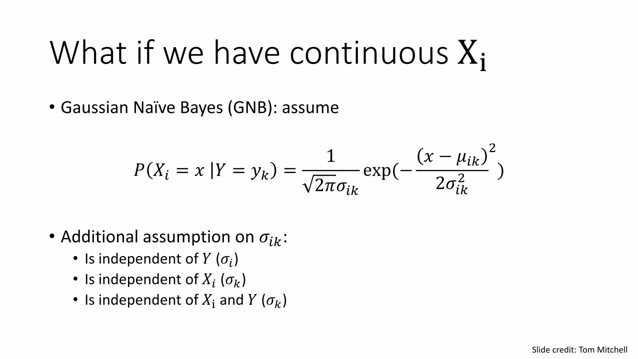
What if we have continuous Xi• Gaussian Naïve Bayes (GNB): assume

𝑃 𝑋𝑖 = 𝑥 𝑌 = 𝑦𝑘 =1

2𝜋𝜎𝑖𝑘exp(−

𝑥 − 𝜇𝑖𝑘

2𝜎𝑖𝑘2

2

)

• Additional assumption on 𝜎𝑖𝑘:• Is independent of 𝑌 (𝜎𝑖)

• Is independent of 𝑋𝑖 (𝜎𝑘)

• Is independent of 𝑋i and 𝑌 (𝜎𝑘)


Naïve Bayes algorithm – continuous Xi

• For each value ykEstimate 𝜋𝑘 = 𝑃(𝑌 = 𝑦𝑘)

For each attribute Xi estimate

Class conditional mean 𝜇𝑖𝑘, variance 𝜎𝑖𝑘

• Classify Xtest


𝑃 𝑌 = 𝑦𝑘 Π𝑖𝑃 𝑋𝑖test 𝑌 = 𝑦𝑘)


𝜋𝑘 Π𝑖 𝑁𝑜𝑟𝑚𝑎𝑙(𝑋𝑖test, 𝜇𝑖𝑘, 𝜎𝑖𝑘)


Things to remember


• Estimating parameters from data• Maximum likelihood (ML) maximize 𝑃(Data|𝜃)

• Maximum a posteriori estimation (MAP) maximize 𝑃(𝜃|Data)

•Naive Bayes𝑃 𝑌 = 𝑦𝑘 𝑋1, ⋯ , 𝑋𝑛) ∝ 𝑃 𝑌 = 𝑦𝑘 Π𝑖𝑃 𝑋𝑖 𝑌 = 𝑦𝑘)

Next class

• Logistic regression

Documents

Naïve Bayes - filebox.ece.vt.edujbhuang/teaching/ECE5424-CS5824/sp19/slides/Lec04.pdf · •Naive Bayes. Random variables •Outcome space S •Space of possible outcomes •Random