Embed Size (px)
Citation preview

Naïve Bayes
Robot Image Credit: Viktoriya Sukhanova © 123RF.com
These slides were assembled by Eric Eaton, with grateful acknowledgement of the many others who made their course materials freely available online. Feel free to reuse or adapt these slides for your own academic purposes, provided that you include proper attribution. Please send comments and corrections to Eric.

Essential Probability Concepts• Marginalization:
• Conditional Probability:
• Bayes’ Rule:
• Independence:
2
P (A | B) =P (A ^B)
P (B)
P (A ^B) = P (A | B)⇥ P (B)
A??B $ P (A ^B) = P (A)⇥ P (B)
$ P (A | B) = P (A)
P (A | B) =P (B | A)⇥ P (A)
P (B)
A??B | C $ P (A ^B | C) = P (A | C)⇥ P (B | C)
P (B) =X
v2values(A)
P (B ^A = v)

Density Estimation
3

Recall the Joint Distribution...
4
alarm ¬alarmearthquake ¬earthquake earthquake ¬earthquake
burglary 0.01 0.08 0.001 0.009¬burglary 0.01 0.09 0.01 0.79

How Can We Obtain a Joint Distribution?Option 1: Elicit it from an expert human
Option 2: Build it up from simpler probabilistic facts• e.g, if we knew
P(a) = 0.7 P(b|a) = 0.2 P(b|¬a) = 0.1then, we could compute P(a Ù b)
Option 3: Learn it from data...
5Based on slide by Andrew Moore

Learning a Joint Distribution
Build a JD table for your attributes in which the probabilities are unspecified
Then, fill in each row with:
records ofnumber totalrow matching records)row(ˆ =P
A B C Prob0 0 0 ?
0 0 1 ?
0 1 0 ?
0 1 1 ?
1 0 0 ?
1 0 1 ?
1 1 0 ?
1 1 1 ?
A B C Prob0 0 0 0.30
0 0 1 0.05
0 1 0 0.10
0 1 1 0.05
1 0 0 0.05
1 0 1 0.10
1 1 0 0.25
1 1 1 0.10
Fraction of all records in whichA and B are true but C is false
Step 1: Step 2:
Slide © Andrew Moore

Example of Learning a Joint PDThis Joint PD was obtained by learning from three attributes in the UCI “Adult” Census Database [Kohavi 1995]
Slide © Andrew Moore

Density Estimation• Our joint distribution learner is an example of something called Density Estimation
• A Density Estimator learns a mapping from a set of attributes to a probability
DensityEstimator
ProbabilityInputAttributes
Slide © Andrew Moore

RegressorPrediction of real-‐valued output
InputAttributes
Density Estimation
Compare it against the two other major kinds of models:
ClassifierPrediction of categorical output
InputAttributes
DensityEstimator
ProbabilityInputAttributes
Slide © Andrew Moore

Evaluating Density Estimation
Test set Accuracy
?
Test set Accuracy
Test-‐set criterion for estimating performance
on future data
RegressorPrediction of real-‐valued output
InputAttributes
ClassifierPrediction of categorical output
InputAttributes
DensityEstimator
ProbabilityInputAttributes
Slide © Andrew Moore

• Given a record x, a density estimator M can tell you how likely the record is:
• The density estimator can also tell you how likely the dataset is:– Under the assumption that all records were independentlygenerated from the Density Estimator’s JD (that is, i.i.d.)
Evaluating a Density Estimator
P̂ (x | M)
P̂ (dataset | M) = P̂ (x1 ^ x2 ^ . . . ^ xn | M) =nY
i=1
P̂ (xi | M)
dataset
Slide by Andrew Moore

Example Small Dataset: Miles Per GallonFrom the UCI repository (thanks to Ross Quinlan)• 192 records in the training set
mpg modelyear maker
good 75to78 asiabad 70to74 americabad 75to78 europebad 70to74 americabad 70to74 americabad 70to74 asiabad 70to74 asiabad 75to78 america: : :: : :: : :bad 70to74 americagood 79to83 americabad 75to78 americagood 79to83 americabad 75to78 americagood 79to83 americagood 79to83 americabad 70to74 americagood 75to78 europebad 75to78 europe
P̂ (dataset | M) =nY
i=1
P̂ (xi | M)
= 3.4⇥ 10�203 (in this case)
Slide by Andrew Moore
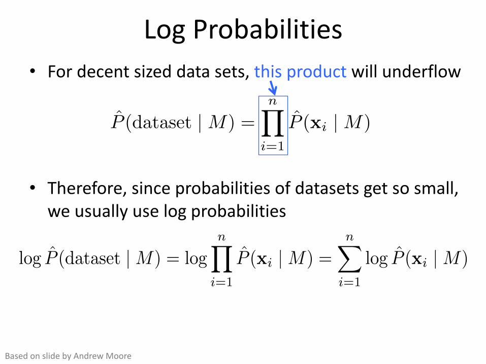
Log Probabilities• For decent sized data sets, this product will underflow
• Therefore, since probabilities of datasets get so small, we usually use log probabilities
log
ˆP (dataset | M) = log
nY
i=1
ˆP (xi | M) =
nX
i=1
log
ˆP (xi | M)
P̂ (dataset | M) =nY
i=1
P̂ (xi | M)
= 3.4⇥ 10�203 (in this case)
Based on slide by Andrew Moore

Example Small Dataset: Miles Per GallonFrom the UCI repository (thanks to Ross Quinlan)• 192 records in the training set
mpg modelyear maker
good 75to78 asiabad 70to74 americabad 75to78 europebad 70to74 americabad 70to74 americabad 70to74 asiabad 70to74 asiabad 75to78 america: : :: : :: : :bad 70to74 americagood 79to83 americabad 75to78 americagood 79to83 americabad 75to78 americagood 79to83 americagood 79to83 americabad 70to74 americagood 75to78 europebad 75to78 europe
Slide by Andrew Moore
log
ˆP (dataset | M) =
nX
i=1
log
ˆP (xi | M)
= �466.19 (in this case)

Pros/Cons of the Joint Density EstimatorThe Good News:• We can learn a Density Estimator from data.• Density estimators can do many good things…– Can sort the records by probability, and thus spot weird records (anomaly detection)
– Can do inference– Ingredient for Bayes Classifiers (coming very soon...)
The Bad News:• Density estimation by directly learning the joint is impractical, may result in adverse behavior
Slide by Andrew Moore

Curse of Dimensionality
Slide by Christopher Bishop

The Joint Density Estimator on a Test Set
• An independent test set with 196 cars has a much worse log-‐likelihood– Actually it’s a billion quintillion quintillion quintillion quintillion times less likely
• Density estimators can overfit......and the full joint density estimator is the overfittiest of them all!
Slide by Andrew Moore

Copyright © Andrew W. Moore
Overfitting Density Estimators
If this ever happens, the joint PDE learns there are certain combinations that are impossible
log
ˆP (dataset | M) =
nX
i=1
log
ˆP (xi | M)
= �1 if for any i, ˆP (xi | M) = 0
Slide by Andrew Moore

The Joint Density Estimator on a Test Set
• The only reason that the test set didn’t score -‐∞ is that the code was hard-‐wired to always predict a probability of at least 1/1020
Slide by Andrew Moore

The Naïve Bayes Classifier
21

Bayes’ Rule• Recall Baye’s Rule:
• Equivalently, we can write:
where X is a random variable representing the evidence and Y is a random variable for the label
• This is actually short for:
where Xj denotes the random variable for the j th feature22
P (hypothesis | evidence) = P (evidence | hypothesis)⇥ P (hypothesis)
P (evidence)
P (Y = yk | X = xi) =P (Y = yk)P (X1 = xi,1 ^ . . . ^Xd = xi,d | Y = yk)
P (X1 = xi,1 ^ . . . ^Xd = xi,d)
P (Y = yk | X = xi) =P (Y = yk)P (X = xi | Y = yk)
P (X = xi)

Naïve Bayes ClassifierIdea: Use the training data to estimate
Then, use Bayes rule to infer for new data
• Estimating the joint probability distribution is not practical
23
P (X | Y ) P (Y )and .P (Y |Xnew)
P (Y = yk | X = xi) =P (Y = yk)P (X1 = xi,1 ^ . . . ^Xd = xi,d | Y = yk)
P (X1 = xi,1 ^ . . . ^Xd = xi,d)
P (X1, X2, . . . , Xd | Y )
Easy to estimate from data
Unnecessary, as it turns out
Impractical, but necessary

Naïve Bayes ClassifierProblem: estimating the joint PD or CPD isn’t practical– Severely overfits, as we saw before
However, if we make the assumption that the attributes are independent given the class label, estimation is easy!
• In other words, we assume all attributes are conditionally independent given Y
• Often this assumption is violated in practice, but more on that later…
24
P (X1, X2, . . . , Xd | Y ) =dY
j=1
P (Xj | Y )

Training Naïve BayesEstimate and directly from the training data by counting!
P(play) = ? P(¬play) = ?P(Sky = sunny | play) = ? P(Sky = sunny | ¬play) = ?P(Humid = high | play) = ? P(Humid = high | ¬play) = ?... ...
25
Sky Temp Humid Wind Water Forecast Play?sunny warm normal strong warm same yessunny warm high strong warm same yesrainy cold high strong warm change nosunny warm high strong cool change yes
P (Xj | Y ) P (Y )

Training Naïve BayesEstimate and directly from the training data by counting!
P(play) = ? P(¬play) = ?P(Sky = sunny | play) = ? P(Sky = sunny | ¬play) = ?P(Humid = high | play) = ? P(Humid = high | ¬play) = ?... ...
26
Sky Temp Humid Wind Water Forecast Play?sunny warm normal strong warm same yessunny warm high strong warm same yesrainy cold high strong warm change nosunny warm high strong cool change yes
P (Xj | Y ) P (Y )

Training Naïve BayesEstimate and directly from the training data by counting!
P(play) = 3/4 P(¬play) = 1/4P(Sky = sunny | play) = ? P(Sky = sunny | ¬play) = ?P(Humid = high | play) = ? P(Humid = high | ¬play) = ?... ...
27
Sky Temp Humid Wind Water Forecast Play?sunny warm normal strong warm same yessunny warm high strong warm same yesrainy cold high strong warm change nosunny warm high strong cool change yes
P (Xj | Y ) P (Y )

Training Naïve BayesEstimate and directly from the training data by counting!
P(play) = 3/4 P(¬play) = 1/4P(Sky = sunny | play) = ? P(Sky = sunny | ¬play) = ?P(Humid = high | play) = ? P(Humid = high | ¬play) = ?... ...
28
Sky Temp Humid Wind Water Forecast Play?sunny warm normal strong warm same yessunny warm high strong warm same yesrainy cold high strong warm change nosunny warm high strong cool change yes
P (Xj | Y ) P (Y )

Training Naïve BayesEstimate and directly from the training data by counting!
P(play) = 3/4 P(¬play) = 1/4P(Sky = sunny | play) = 1 P(Sky = sunny | ¬play) = ?P(Humid = high | play) = ? P(Humid = high | ¬play) = ?... ...
29
Sky Temp Humid Wind Water Forecast Play?sunny warm normal strong warm same yessunny warm high strong warm same yesrainy cold high strong warm change nosunny warm high strong cool change yes
P (Xj | Y ) P (Y )

Training Naïve BayesEstimate and directly from the training data by counting!
P(play) = 3/4 P(¬play) = 1/4P(Sky = sunny | play) = 1 P(Sky = sunny | ¬play) = ?P(Humid = high | play) = ? P(Humid = high | ¬play) = ?... ...
30
Sky Temp Humid Wind Water Forecast Play?sunny warm normal strong warm same yessunny warm high strong warm same yesrainy cold high strong warm change nosunny warm high strong cool change yes
P (Xj | Y ) P (Y )

Training Naïve BayesEstimate and directly from the training data by counting!
P(play) = 3/4 P(¬play) = 1/4P(Sky = sunny | play) = 1 P(Sky = sunny | ¬play) = 0P(Humid = high | play) = ? P(Humid = high | ¬play) = ?... ...
31
Sky Temp Humid Wind Water Forecast Play?sunny warm normal strong warm same yessunny warm high strong warm same yesrainy cold high strong warm change nosunny warm high strong cool change yes
P (Xj | Y ) P (Y )

Training Naïve BayesEstimate and directly from the training data by counting!
P(play) = 3/4 P(¬play) = 1/4P(Sky = sunny | play) = 1 P(Sky = sunny | ¬play) = 0P(Humid = high | play) = ? P(Humid = high | ¬play) = ?... ...
32
Sky Temp Humid Wind Water Forecast Play?sunny warm normal strong warm same yessunny warm high strong warm same yesrainy cold high strong warm change nosunny warm high strong cool change yes
P (Xj | Y ) P (Y )

Training Naïve BayesEstimate and directly from the training data by counting!
P(play) = 3/4 P(¬play) = 1/4P(Sky = sunny | play) = 1 P(Sky = sunny | ¬play) = 0P(Humid = high | play) = 2/3 P(Humid = high | ¬play) = ?... ...
33
Sky Temp Humid Wind Water Forecast Play?sunny warm normal strong warm same yessunny warm high strong warm same yesrainy cold high strong warm change nosunny warm high strong cool change yes
P (Xj | Y ) P (Y )

Training Naïve BayesEstimate and directly from the training data by counting!
P(play) = 3/4 P(¬play) = 1/4P(Sky = sunny | play) = 1 P(Sky = sunny | ¬play) = 0P(Humid = high | play) = 2/3 P(Humid = high | ¬play) = ?... ...
34
Sky Temp Humid Wind Water Forecast Play?sunny warm normal strong warm same yessunny warm high strong warm same yesrainy cold high strong warm change nosunny warm high strong cool change yes
P (Xj | Y ) P (Y )

Training Naïve BayesEstimate and directly from the training data by counting!
P(play) = 3/4 P(¬play) = 1/4P(Sky = sunny | play) = 1 P(Sky = sunny | ¬play) = 0P(Humid = high | play) = 2/3 P(Humid = high | ¬play) = 1... ...
35
Sky Temp Humid Wind Water Forecast Play?sunny warm normal strong warm same yessunny warm high strong warm same yesrainy cold high strong warm change nosunny warm high strong cool change yes
P (Xj | Y ) P (Y )

Training Naïve BayesEstimate and directly from the training data by counting!
P(play) = 3/4 P(¬play) = 1/4P(Sky = sunny | play) = 1 P(Sky = sunny | ¬play) = 0P(Humid = high | play) = 2/3 P(Humid = high | ¬play) = 1... ...
36
Sky Temp Humid Wind Water Forecast Play?sunny warm normal strong warm same yessunny warm high strong warm same yesrainy cold high strong warm change nosunny warm high strong cool change yes
P (Xj | Y ) P (Y )

Laplace Smoothing• Notice that some probabilities estimated by counting might be zero– Possible overfitting!
• Fix by using Laplace smoothing:– Adds 1 to each count
where – cv is the count of training instances with a value of v for
attribute j and class label yk– |values(Xj)| is the number of values Xj can take on
37
P (Xj = v | Y = yk) =cv + 1X
v02values(Xj)
cv0 + |values(Xj)|

Training Naïve Bayes with Laplace SmoothingEstimate and directly from the training data by counting with Laplace smoothing:
P(play) = 3/4 P(¬play) = 1/4P(Sky = sunny | play) = 4/5 P(Sky = sunny | ¬play) = ?P(Humid = high | play) = ? P(Humid = high | ¬play) = ?... ...
38
Sky Temp Humid Wind Water Forecast Play?sunny warm normal strong warm same yessunny warm high strong warm same yesrainy cold high strong warm change nosunny warm high strong cool change yes
P (Xj | Y ) P (Y )

Training Naïve Bayes with Laplace SmoothingEstimate and directly from the training data by counting with Laplace smoothing:
P(play) = 3/4 P(¬play) = 1/4P(Sky = sunny | play) = 4/5 P(Sky = sunny | ¬play) = 1/3P(Humid = high | play) = ? P(Humid = high | ¬play) = ?... ...
39
Sky Temp Humid Wind Water Forecast Play?sunny warm normal strong warm same yessunny warm high strong warm same yesrainy cold high strong warm change nosunny warm high strong cool change yes
P (Xj | Y ) P (Y )

Training Naïve Bayes with Laplace SmoothingEstimate and directly from the training data by counting with Laplace smoothing:
P(play) = 3/4 P(¬play) = 1/4P(Sky = sunny | play) = 4/5 P(Sky = sunny | ¬play) = 1/3P(Humid = high | play) = 3/5 P(Humid = high | ¬play) = ?... ...
40
Sky Temp Humid Wind Water Forecast Play?sunny warm normal strong warm same yessunny warm high strong warm same yesrainy cold high strong warm change nosunny warm high strong cool change yes
P (Xj | Y ) P (Y )
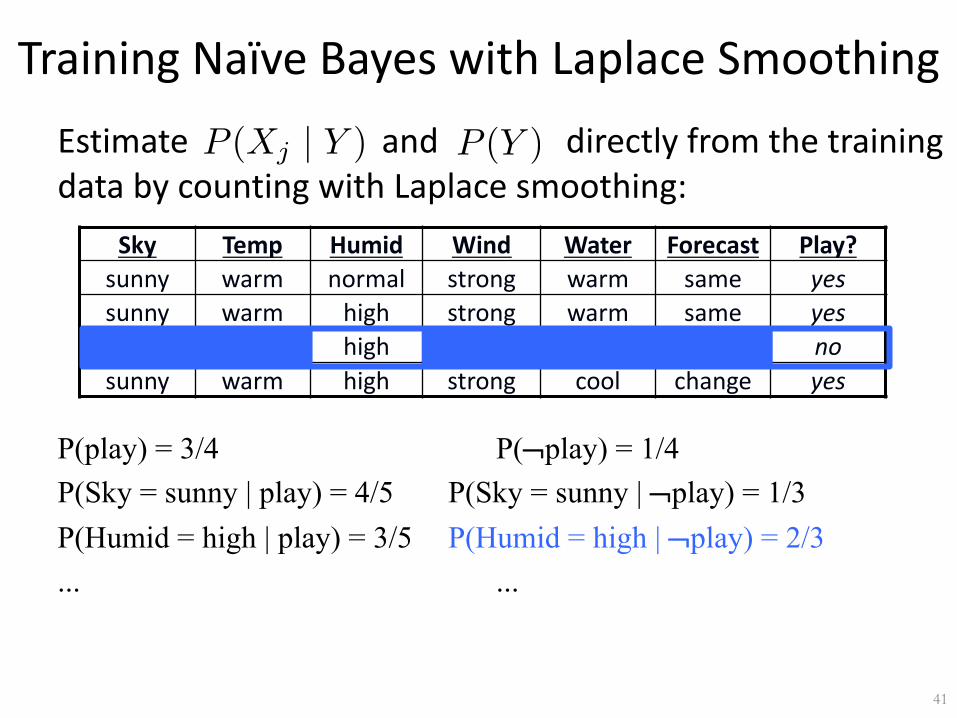
Training Naïve Bayes with Laplace SmoothingEstimate and directly from the training data by counting with Laplace smoothing:
P(play) = 3/4 P(¬play) = 1/4P(Sky = sunny | play) = 4/5 P(Sky = sunny | ¬play) = 1/3P(Humid = high | play) = 3/5 P(Humid = high | ¬play) = 2/3... ...
41
Sky Temp Humid Wind Water Forecast Play?sunny warm normal strong warm same yessunny warm high strong warm same yesrainy cold high strong warm change nosunny warm high strong cool change yes
P (Xj | Y ) P (Y )

Using the Naïve Bayes Classifier• Now, we have
– In practice, we use log-‐probabilities to prevent underflow
• To classify a new point x,
42
P (Y = yk | X = xi) =P (Y = yk)
Qdj=1 P (Xj = xi,j | Y = yk)
P (X = xi)This is constant for a given instance, and so irrelevant to our prediction
h(x) = argmax
yk
P (Y = yk)
dY
j=1
P (Xj = xj | Y = yk)
= argmax
yk
logP (Y = yk) +
dX
j=1
logP (Xj = xj | Y = yk)
j th attribute value of x
h(x) = argmax
yk
P (Y = yk)
dY
j=1
P (Xj = xj | Y = yk)
= argmax
yk
logP (Y = yk) +
dX
j=1
logP (Xj = xj | Y = yk)

43
The Naïve Bayes Classifier Algorithm
• For each class label yk– Estimate P(Y = yk) from the data– For each value xi,j of each attribute Xi
• Estimate P(Xi = xi,j | Y = yk)
• Classify a new point via:
• In practice, the independence assumption doesn’t often hold true, but Naïve Bayes performs very well despite this
h(x) = argmax
yk
logP (Y = yk) +
dX
j=1
logP (Xj = xj | Y = yk)

Computing Probabilities(Not Just Predicting Labels)
• NB classifier gives predictions, not probabilities, because we ignore P(X) (the denominator in Bayes rule)
• Can produce probabilities by:– For each possible class label yk , compute
– α is given by
– Class probability is given by
44
P̃ (Y = yk | X = x) = P (Y = yk)dY
j=1
P (Xj = xj | Y = yk)
This is the numerator of Bayes rule, and is therefore off the true probability by a factor
of α that makes probabilities sum to 1
↵ =1
P#classesk=1 P̃ (Y = yk | X = x)
P (Y = yk | X = x) = ↵P̃ (Y = yk | X = x)

Naïve Bayes Applications• Text classification– Which e-‐mails are spam?– Which e-‐mails are meeting notices?– Which author wrote a document?
• Classifying mental states
People Words Animal Words
Learning P(BrainActivity | WordCategory)
Pairwise ClassificationAccuracy: 85%

The Naïve Bayes Graphical Model
• Nodes denote random variables• Edges denote dependency• Each node has an associated conditional probability table (CPT), conditioned upon its parents
46
Attributes (evidence)
Labels (hypotheses)
…
Y
X1 Xi Xd…
P(Y)
P(X1 | Y) P(Xi | Y) P(Xd | Y)

Example NB Graphical Model
47
…
Play
Sky Temp Humid…
Sky Temp Humid Play?sunny warm normal yessunny warm high yesrainy cold high nosunny warm high yes
Data:

Example NB Graphical Model
48
…
Play
Sky Temp Humid…
Sky Temp Humid Play?sunny warm normal yessunny warm high yesrainy cold high nosunny warm high yes
Play? P(Play)yesno
Data:

Example NB Graphical Model
49
…
Play
Sky Temp Humid…
Sky Temp Humid Play?sunny warm normal yessunny warm high yesrainy cold high nosunny warm high yes
Play? P(Play)yes 3/4no 1/4
Data:

Example NB Graphical Model
50
…
Play
Sky Temp Humid…
Sky Temp Humid Play?sunny warm normal yessunny warm high yesrainy cold high nosunny warm high yes
Play? P(Play)yes 3/4no 1/4
Sky Play? P(Sky | Play)sunny yesrainy yessunny norainy no
Data:
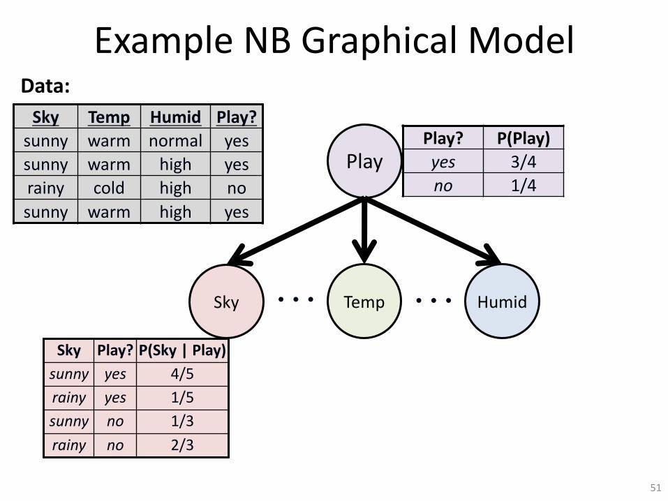
Example NB Graphical Model
51
…
Play
Sky Temp Humid…
Sky Temp Humid Play?sunny warm normal yessunny warm high yesrainy cold high nosunny warm high yes
Play? P(Play)yes 3/4no 1/4
Sky Play? P(Sky | Play)sunny yes 4/5rainy yes 1/5sunny no 1/3rainy no 2/3
Data:

Example NB Graphical Model
52
…
Play
Sky Temp Humid…
Sky Temp Humid Play?sunny warm normal yessunny warm high yesrainy cold high nosunny warm high yes
Play? P(Play)yes 3/4no 1/4
Sky Play? P(Sky | Play)sunny yes 4/5rainy yes 1/5sunny no 1/3rainy no 2/3
Temp Play? P(Temp | Play)warm yescold yeswarm nocold no
Data:

Example NB Graphical Model
53
…
Play
Sky Temp Humid…
Sky Temp Humid Play?sunny warm normal yessunny warm high yesrainy cold high nosunny warm high yes
Play? P(Play)yes 3/4no 1/4
Sky Play? P(Sky | Play)sunny yes 4/5rainy yes 1/5sunny no 1/3rainy no 2/3
Temp Play? P(Temp | Play)warm yes 4/5cold yes 1/5warm no 1/3cold no 2/3
Data:
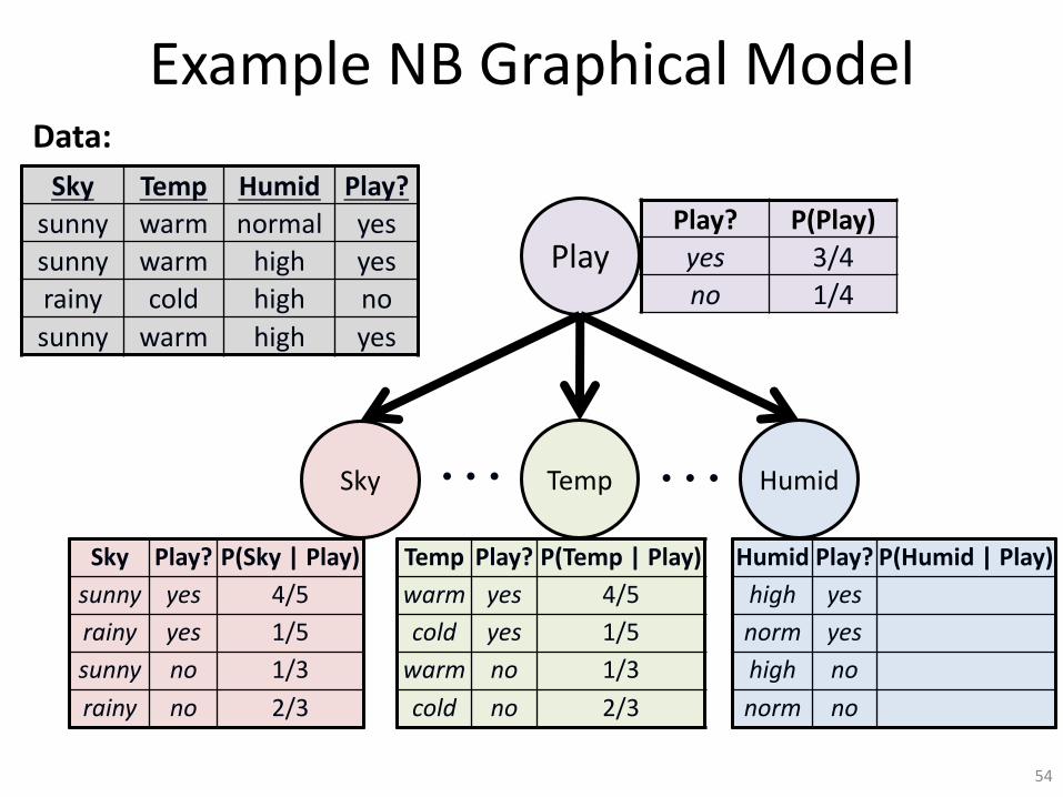
Example NB Graphical Model
54
…
Play
Sky Temp Humid…
Sky Temp Humid Play?sunny warm normal yessunny warm high yesrainy cold high nosunny warm high yes
Play? P(Play)yes 3/4no 1/4
Sky Play? P(Sky | Play)sunny yes 4/5rainy yes 1/5sunny no 1/3rainy no 2/3
Temp Play? P(Temp | Play)warm yes 4/5cold yes 1/5warm no 1/3cold no 2/3
Humid Play? P(Humid | Play)high yesnorm yeshigh nonorm no
Data:

Example NB Graphical Model
55
…
Play
Sky Temp Humid…
Sky Temp Humid Play?sunny warm normal yessunny warm high yesrainy cold high nosunny warm high yes
Play? P(Play)yes 3/4no 1/4
Sky Play? P(Sky | Play)sunny yes 4/5rainy yes 1/5sunny no 1/3rainy no 2/3
Temp Play? P(Temp | Play)warm yes 4/5cold yes 1/5warm no 1/3cold no 2/3
Humid Play? P(Humid | Play)high yes 3/5norm yes 2/5high no 2/3norm no 1/3
Data:

Example Using NB for Classification
Goal: Predict label for x = (rainy, warm, normal)56
…
Play
Sky Temp Humid
…
Play? P(Play)yes 3/4no 1/4
Sky Play? P(Sky | Play)sunny yes 4/5rainy yes 1/5sunny no 1/3rainy no 2/3
Temp Play? P(Temp | Play)warm yes 4/5cold yes 1/5warm no 1/3cold no 2/3
Humid Play? P(Humid | Play)high yes 3/5norm yes 2/5high no 2/3norm no 1/3
h(x) = argmax
yk
logP (Y = yk) +
dX
j=1
logP (Xj = xj | Y = yk)

Example Using NB for Classification
Predict label for: x = (rainy, warm, normal)
57
…
Play
Sky Temp Humid
…
Play? P(Play)yes 3/4no 1/4
Sky Play? P(Sky | Play)sunny yes 4/5rainy yes 1/5sunny no 1/3rainy no 2/3
Temp Play? P(Temp | Play)warm yes 4/5cold yes 1/5warm no 1/3cold no 2/3
Humid Play? P(Humid | Play)high yes 3/5norm yes 2/5high no 2/3norm no 1/3
predict PLAY

Naïve Bayes SummaryAdvantages:• Fast to train (single scan through data)• Fast to classify • Not sensitive to irrelevant features• Handles real and discrete data• Handles streaming data well
Disadvantages:• Assumes independence of features
58Slide by Eamonn Keogh