3DGRAPE/AL:

N95- 28750

THE AMES / LANGLEY TECHNOLOGY UPGRADE

Reese L. Sorenson

National Aeronautics and Space AdministrationAmes Research Center

Moffett Field, CA 94035-1000

Stephen J. AlterLockheed Engineering & Sciences Co.

Langley Research CenterHampton, VA 23666

SUMMARY

This paper describes a new three-dimensional structured multiple-block volume grid generator called3DGRAPE/AL. It is a significantly improved version of the previously-released and widely-distributed program3DGRAPE, with many of the improvements taken from the grid-generator program 3DMAGGS 1. It generatesvolume grids by iteratively solving the Poisson Equations in three-dimensions. The right-hand-side terms aredesigned so that user-specified grid cell heights and user-specified grid cell skewness near boundary surfacesresult automatically, with little user intervention. Versatility was a high priority in this code's development, andas a result it can generate grids in almost any three-dimensional physical domain. Improvements include addedkinds of forcing functions, improved control of cell skewness, improved initial conditions, convergenceacceleration, the ability to take as input the output from GRIDGEN, and a simple but powerful graphical userinterface(GUI).

INTRODUCTION/

/

The original program, 3DGRAPE 2 ,3, of which 3DGRAPE/AL is an updated version, is a batch-typeprogram. It reads in pre-defined input data, generates the grid, and writes it out. For those boundary surfaceswhich are of interest (i.e., the body) it expects to read X,Y,Z coordinates of surface grid points which the user haspre-defined using other software. Other boundary surfaces of less interest (i.e., the outer boundary) can be foundby the program itself using simple analytic shapes. The grid can consist of multiple blocks, and the program iscapable of finding its own intemal block-to-block boundary surfaces. Volume grid points are found bynumerically solving the Poisson equations. The Steger & Sorenson (S&S) Right-Hand-Side (RHS) terms (i.e.,forcing functions) in those equations are of a type which allows the user to choose the desired cell height on aread-in boundary, after which the program automatically finds the actual numerical values for the RHS termswhich yield the desired cell heights. In the process the RHS terms attempt to give local near-orthogonality in theregion of those same read-in surfaces. The cell heights the user requires may be of any magnitude (limited onlyby the precision of the computer), appropriate for both viscous and inviscid aerodynamic flow modeling. Theinput data is ordinary text, with required formatting. The output grid may be any of three formats, including thecommonly used PLOT3D 4 formats.

All the features described above for the original program are preserved in the new program, and asignificant suite of new features is added. Those new features include:

• Grid quality is enhanced by re-formulated Steger & Sorenson (S&S) control terms in the PoissonEquations. The user may specify arbitrary angles with which lines are to intersect boundaries, rather thanthat specification being limited to 90 ° everywhere. The treatment of sharp comers which transverseboundary surfaces (e.g., a grid wrapping around an airplane fuselage which has a strake) is improvedusing this capability.

• Another improvement to grid quality is the addition of Thomas & Middlecoff (T&M) clustering terms forcases where all six faces of a block are read-in, as found in GRIDGEN and 3DMAGGS. The user canchoose either the Steger & Sorenson terms (as in the original code and improved as described above), the

447

https://ntrs.nasa.gov/search.jsp?R=19950022329 2018-06-27T21:45:33+00:00Z

Thomas& Middlecofftypeterms,orablendingbetweenthetwowhichgivesgoodcell-sizeandskewnesscontrolatboththeboundariesandtheinterior.

• Gridqualityisevaluatedbycomputingandprintingmaxima,minima,medians,andaveragesof cellheightsandnon-orthogonality,atboundariesandin theinteriorsof theblocksof thefinishedgrid.

• Initializationis improvedbyTrans-FiniteInterpolation5(forcaseswithsix fixedboundarysurfaces).Insomecasesgridsinitializedthuslycanserveasthefinalgrid,inothersthisimprovedinitializationspeedsconvergence.

• Erlich'sAdHocMethodforcomputinglocallyoptimumrelaxationparametersis availableforthecode'sSORsolver.Thisalsocanaccelerateconvergence

• WheninstalledonCRAYcomputersthecodeisvectorizedin allthreecoordinatedirections,allowingthelongestpossiblevectorlengthineachblock.This,too,acceleratesconvergence.

• Thegridgenerationiterationschedulecanbedividedintopans.Parameterswhicheffectconvergence(suchasrelaxationrates),aswellasthetypeof clusteringtermsusedandtheirassociateddecayrates,areadjustablewitheachpart. Intermediatesolutionsandrestartfilescanbewrittenaftereachpart.Thus,inpracticaloperation,asmuchcansometimesbeaccomplishedinonerunwiththisprogramasinmultipleruns with other grid generators.

• An input filter called PREGRAPE/AL, taken from 3DMAGGS, is supplied as a companion program. It

inputs the output from the GRIDGEN 6 code, which contains blocking strategy and surface grids, andturns that into input for 3DGRAPE/AL.

• Required cell heights and skewness at read-in surfaces can be specified by the user at each point from afile. One possible application of the ability to specify the skewness at each point is in hypersonic flowwhere in the exit plane near the shock the flow is aligned with the shock and so should be the grid, whilein that same face near the body the grid should be aligned with the body surface, and the angles areblended in-between.

• A complete grid generated elsewhere can be read-in, and the elliptic solver can be run a few steps tosmooth the grid.

• A Graphical User Interface, coded in FORTRAN-77 and calling the IRIS Graphics Library, allows theuser to watch selected grid surfaces while the grid solver is iterating. A full suite of transforms and otherfeatures is included.

The code is written in FORTRAN-77. It can be installed as an ordinary batch program, and in that form itshould run on almost any computer. Alternately, on a Silicon Graphics Inc. (SGI) workstation it can be installedalong with its graphical user interface. The GUI is also written in FORTRAN-77, and calls functions in the IRISGraphics Librau,. For compiling on a CRAY supercompuler there is a vectorized batch version.

THEORETICAL DEVELOPMENT OF THE POISSON EQUATIONS IN PHYSICAL SPACE

The original 3DGRAPE program, the 3DMAGGS program, and the new 3DGRAPE/AL program allgenerate grids by iteratively solving the Poisson Equalions in three-dimensions. A mapping is thus found

between the computational coordinates _,rl,_ and the physical coordinates X,Y,Z. The equations are typically

given in the computational space as

_xx -1- _yy "+" _zz- P(g, rl,g)

_xx "}" lqyy + l']zz = Q(_,I*I,_)

_xx "b _yy "1- _'?zz----R(%,rl,g)

(la)

(lb)

(lc)

448

However,it isnaturalto applythemin thephysicalspace.It isnaturaltospecifythegridboundaryconditionsbygivingX,Y,Zatfixedvaluesof _,rl,_ratherthanto givevaluesof _,rl,_atfixedvaluesof X,Y,Z.Thetransformationof Eqs.1tophysicalspaceproceedsasfollows.Clearly,wemusthave

(2a)

(2b)

= _(x,y,z)

To effectthistransformationwe must alsohave

(2c)

x = ) (3a)

y = y(q,rl,, ) (3b)

t'__ __

z = zq q,q,Differentiating Eqs. 2 and applying the chain rule gives

(3c)

d_ _x _y _z

OTI = lqx qy qz

dE _x _y _z

Likewise, differentiating Eqs. 3 and applying the chain rule gives

OX

dydz

(4)

= Y_ Yn Y; drl _s)

z_ zn z; dE

We designate the 3 x 3 matrix in Eq. 5 as M, assume that its inverse exists, and pre-multiply both sides of Eq. 5by M - 1. This gives

M-1 =

.w

IOta,,.

(6)

Substituting from Eq. 6 into Eq. 4 gives

449

M-1

We know that, in general, if

and if B -1 exists then

Therefore it must be true that

Pre-multiplying by B gives

Applying Eqs. 8 to Eq. 7 gives

_x _y _z

Tlx lqy lqz

Cx Cy Cz

(7)

A_ = B _ (8a)

m _._B -1 v = v (8b)

B -1 A = I (8c)

A = B (8d)

lqx qy lqz

Cx Cy Cz

For this to be useful, we must find M -1 . It is known, in general, that

(9)

A_1 Adj(A)-- (lo)Det(A)

Where Adj(A) is the adjoint of A and Det(A) is the determinant of A. The adjoint of A is a matrix having as eachelement the corresponding cofactor of A. Thus, from Eq. 9, we have

(11)

1'_11 'Y12 _13 /

- 1721 '::7:3 J]_31 '/32_331

_x _y _z

qx qy qz

CxCyCzwhere _ij is the ij-th cofactor of M and J is the determinant of M. By inspection of Eq. 11 we see that

_x ---- Tl I/J (12a)

Cy = _12/J (12b)

450

_z = 'Y13/J (12c)

1Ix = _t21/J (12d)

'Fly = 'Y22/J (12e)

rlz = 723/J (120

_x = _t31/J (12g)

_y = 'y3JJ (12h)

_z = _33/J (12i)

Completion of the derivation of the transformed Poisson equations requires further differentiating themetrics in Eqs. 12, substituting them into Eqs. 1, and collecting terms. This process is simple calculus, but verylengthy and beyond the scope of this paper. The result is

+ 2 ( otl2?_n + 13_13r'_; -I- O_2frl0 (13a)

= _j2 (PF_ + Q?n + R;;)where:

and

(13b)

(13c)

THEORETICAL DEVELOPMENT OF IMPROVED S&S RHS TERMS

The distribution of points in the grid results primarily from the influence of the Right-Hand Side (RHS)terms, or forcing functions. We are free to choose them as we please. In both new and old programs they are:

=+

+

Pl(rl, _)e-a_ + P2(rl, _)e-a(_max-_)

P3(_, _) e-arl + P4(_, _) e-a(rlmax-rl)

Ps(_,rl)e -a; + P6(_, rl)e -a(;max-;)

(14a)

451

Q(_,rl,_) = Ql(rl,_)e a_ +

+ Q3(_,_)e arl +

+ Qs(_,TI)e a; +

Q2(TI, _)e-a(_m_x-_)

Q4(_, _)e-a(rlm_x-_l)

Q6(_,q)e-a(;m_-;)

(14b)

R(_, TI, _) = R l(q, _)e a_ + R2(TI, _)e -a(_m_x-_)

+ R3(_, _)e -arl + R4(_, _)e -a(rlm_x-rl) (14e)

+ Rs(_,rl)e-a; + R6(_,q)e-a(_m_x-_)

Clearly, these RHS terms P,Q,R are simply superpositions of other terms Pn,Qn,Rn for 1___6, multipliedby exponentials which are at their maximum value, one, at the boundary surfaces and which decay with distanceinto the interior of the block. The positive constant "a" in Eqs. 14 is set by the user, and determines the rate ofexponential decay in the size and influence of the RHS terms.

At this point we must introduce a nomenclature for the face numbers. It is seen in Table I. By examiningthat nomenclature we see that at each of the boundaries the terms in P,Q,R having their subscripts equal to theface number are non-zero, and the other terms in P,Q,R approach zero due to the behavior of their exponentialfactors. At face 3, for example, Eqs. 14 reduce to:

= P3(_, _) (15a)

Q(_,rl,_) = Q3(_,_) (15b)

R(%,rl,¢) = R3(_,¢) (,5c)

So then we can find the terms Pn,Qn,Rn at face n by considering each face in tum. At each point on each facewe:

• Assume that the Poisson Equations, Eqs. 13, are satisfied.

• Find values for all first and second partial derivatives required by Eqs. 13.

• Eqs. 13 reduce to a 3 x 3 set of linear equations in the three unknowns Pn,Qn,Rn. Solve them.

Having found all the Pn,Qn,Rn, for 1___6, we can calculate P,Q,R at all points in the grid from Eqs. 14.

However, finding values for all first and second partial derivatives at each face is not trivial. To furtherillustrate this we must restrict our attention to a particular face. We choose face 3 to illustrate. On face 3 the

_ -------) .......@ .......)

derivatives r_, r_, rq;, r_, and can be found by differencing known boundary face points. The derivativesr;;_rlq are found by differencing the grid solution at the current time step, as described on page 78 of Ref. 2. If we

could fred derivatives _rl we could then difference them to find derivatives _ and _.

We find derivatives _)1by adding additional equations which embody the users requirements on cellheight and skewness. In the old 3DGRAPE method we added the three equations

r_. rrl -" 0 (16a)

_rl . r_ = 0 (16b)

452

fq. 2 (16c)

As seen in Table 1, _ and _ vary over face 3, and rl varies along lines intersecting the face. Thus Eqs. 16a and16b require orthogonality between the lines intersecting the face and the coordinate lines running over the face.Eq. 16c requires that the cell height on the surface be the positive constant S.

It is at this point that the old 3DGRAPE method and the new 3DGRAPE/AL method differ. In the newmethod we realize that when making grids about real-world configurations, with singularities and slopediscontinuities, it is sometimes necessary to have grid cells which are skewed in a specified way. Lacking thisability, an inconsistency can develop which can either cause the elliptic solver to not converge, or result in an

And so Eqs. 16 are replaced by

r_, _1]-- r_. _'_cos01

= cos0:

unsuitable grid.

(17a)

(17o)

07c)

where 01 is the angle between the coordinate line intersecting face 3 and the line of varying _ on face 3, and 02 is

the angle between the coordinate line intersecting face 3 and the line of varying _ on face 3. For 01 and 02 equalto 90 °, Eqs. 17 reduce to Eqs. 16.

We now proceed to solve Eqs. 17 for _rl. Expanding, we have

x_x_ + y_ya + z_z_ = c 1 (18a)

x;x_ + y;y_ + z;z_ = c2 (_8b)

X_ + y_ + Z_ = S2 (180where

C1 and c2 are constants because 0 1, 02, S, and the points on face 3 are user-defined inputs. Equations 18 are

three equations in the three unknowns x11,yrl,Zri which are the elements of _rl. But because Eq. 18c is quadratic,

solving this set of equations is not straightforward. We will make an assumption about one of the unknowns andsolve, make that assumption about another of the unknowns and solve, and then make that assumption about thelast of the unknowns and solve. We will then select the answer which is "best."

The first assumption we make is that xrl is a constant. Terms involving xrl in Eqs. 18a and 18b arebrought to the right side of the equations, and then the equations are solved, yielding

Yn = xq722/712 + kl (19a)

Zq = Xrl_32/ _12 + k2 (19b)where

453

k 1 =

k 2 =

K 1 and k2 are constants. Then from Eq. 18c

where

ClZ_ - C2Z _

-712

-b _+4b 2 - 4ac

xn = 2a

a = 1 + (h'22/7,2P+ (_32/_12) 2

b = 21---_2k1')¢12 + k2_32)

c = k_ + k_- S2

The second assumption is that Yrl is a constant. Terms involving Yrl in Eqs. 18a and 18b are brought tothe right side of the equations, and then the equations are solved, yielding

xn = yn_h2/"1(22 + kl

where

Then from Eq. 18c

where

Zrl = YrI'Y32/_22 + k2

ClZ _ - C2Z _

_¢22

C2X _ - ClX _

_22

-b + _/b 2 - 4ac

Yn = 2a

a = 1 + (_,,2/_,22)2 + ('),32/722)2

b- 22{k1_12 + k2_32)

and c is the same as above, in Eq. 20.

(20)

(21a)

(21b)

(22)

454

The third assumption is that z_ is a constant. Terms involving z_ in Eqs. 18a and 18b are brought to theright side of the equations, and then the equations are solved, yielding

Xrl = Zrl'Y12 / '_32 + kl (23a)

where

Yn = zq722 / 732 + k2 (23b)

Then from Eq. 17c

k 2 =

Cly;- c2y_

-732

where

-b + qb 2- 4ac

Z1] = 2a (24)

a = I + (T,JT32) z + (_22/'Y32) 2

b- -_2(k1712 + k2]t22 )

and c is the same as above, in Eq. 20.

In general, none of these three assumptions is strictly correct. However, it usually turns out that at leastone of them is close enough to correct for this method to generate suitable grids. It was said that we wouldchoose whichever of these three solutions was "best." However, Eqs. 20, 22, and 24 each include an ambiguoussign from a square-root operation. Therefore, we actually have six solutions to choose from. Using each of thesix solutions we compute the Jacobian. If the coordinates in the block are right-handed (with the "handedness"being a user-defined input) we choose the solution which yields the largest positive Jacobian. If the coordinatesin the block are left-handed we choose the solution which yields the largest negative Jacobian. The logic behindchoosing based upon the Jacobian is that Jacobians, as defined above, having large absolute values seem to bepresent in grids which are more orthogonal, and, conversely, Jacobians having small absolute values seem to be

present in grids which are highly skewed. Thus the elements of _rl are found.

The foregoing is the analysis for face 3. The analysis for face 4 appears identical, differing only in someof the difference formulas. The analyses for faces !, 2, 5, and 6 follow in a straightforward manner from theforegoing example.

This formulation for the S&S RHS terms requires a lot of computation but most of it is done only once, atthe start of the iteration schedule. It was said, above, that having all values for the derivatives at the face, thosederivatives are substituted into Eqs. 13, yielding a 3 x 3 set of linear equations in the three unknowns Pn,Qn,Rn.

Their solution shows Pn,Qn,Rn to be linear functions of the second derivatives _'rlrl which are found bydifferencing at each time step. The coefficients in those linear functions are fixed for all computational time.

Therefore, the only computation necessary to find the RHS terms in each iteration is to re-evaluate _rm , re-evaluate the linear functions to get Pn,Qn,Rn at each face, and then use Eqs. 14 to re-compute the P,Q,R at everypoint in the grid.

455

Theeffectivenessof thismethodisseeninFigure1. Whenwrappingagridaroundasharpedgeit isnecessaryto causethelinesintersectingthesurfaceneartheedgeto bendtowardtheedgeforbestresults.Theultimateexampleof wrappingagridaroundasharpedgeis towrapit aroundtheedgeof aflat plate.Figure1showsawingwithazero-thicknessextensionin thespanwisedirection,andaC-Htypegridaroundit. Thus,it isnecessaryto wrapaC-type grid around the leading-edge of that wing and its fiat-plate extension. This would nothave been possible with the old type RHS terms.

THOMAS AND MIDDLECOFF CLUSTERING TERMS

When making grids in regions where all six faces of the computational cube are fixed it is sometimesadvantageous to use clustering functions where the spacing normal to a face is determined by the spacing on the

side walls. The Thomas and Middlecoff 7 clustering terms are included here for that purpose. However, theThomas and Middlecoff clustering terms

P = (:I)(V_. V_)

Q = _(Vrl. Vrl)

R = _(V¢. V¢)

rt- r_-.j -_

rn. rnn

v-

where

(25a)

(25b)

(25c)

(25d)

(25e)

f2- ?; ?;;

are given in the computational space, and to be useful here they must be converted to physical space. Applying

the definition of the V operator, illustrated by

V_ = _x] + _yk + _z i (26)

where j, k, and ] are the unit normal vectors, and reducing, gives

Q = V(nx2+ fly2 + 1]2)

R= n(;2x+ #y+Substituting the metrics shown in Eqs. 12 into Eqs. 27, and expanding and re-grouping, gives

(27a)

(27b)

(27c)

456

p = 0[(_. _)(_. _)_ (_. _)]/j20 = v_(_. _)(_. _)-(_. _j2

R- _'-'_[(r_.r_)(_rl,rrl)-(r_,rrl)7J2

(28a)

(28b)

(28c)

These RHS terms generate good grids in many applications. An exception is the situation where theopposing side boundaries, from which the T&M terms are calculated, have very different clusteringcharacteristics. In these cases instabilities in the Poisson solver can result.

It was found in the development of 3DMAGGS that S&S clustering terms tend to give the most-nearly-orthogonal grids near boundaries, while T&M clustering terms give the best clustering in the interior of theblocks. And so a blending between the two kinds of RHS terms was developed, and is included in3DGRAPE/AL.

OPTIMUM RELAXATION PARAMETER

3DGRAPE/AL solves the 3-D Poisson equations using Point Successive Over Relaxation (PSOR). InPSOR there is a relaxation parameter, _, which determines the rate of convergence and stability of the method.In the old program the _ was fixed for all computational time. That option is still available in the new code aswell. However, the new code also has an algorithm to compute an optimum relaxation parameter at every point in

the grid using the method of Erlich. 8

That method requires the equations being solved, here Eq. 13a, to be represented as a difference equationof the following form:

aorj,k,1 + alrj+l,kd + a2rj,k+l,l + a3rj,k,l+l

-" a5rj,k-i,l-" 3. jbi,k,l (29)+ anrj-l,k,l + + a6,j,k,l-I =

Applying standard central differences to all first and second partial derivatives in Eq. 13a, and collecting terms,we arrive at the form of Eq. 29, where

2;2+ao =-2 (A_ (krl

O_ll j2pal - --+ -

(_)2 2A_

(X22 j2Q

a2--(Alq )2 + 2Arl

a 3 -fx33 + J2R

{A_)2 2A;

(30a)

(30b)

(30c)

(306)

457

O_11 j2p (3Oe)

an-(6 )213{22 j2Q (30f)

a5 - (Arl)2 2Arl

0_33 J2R (30g)

a6- (A_)2 2A_

The complex eigenvalues of Eq. 29 at each point, ignoring wave numbers above 1, are

l.t = l-tr + bti = 2( af_7_cos rt + _'a2ascos rt• kmax+lJ max+l (31)

+ (g-3a6cos /1; )lmax+ 1

where I.tr and gi are the real and imaginary parts of g, respectively. It is required that II.t_( 1.

Continuing with Erlich's method, as formulated by Steinbrenner, Chawner, and Fouts on pages 6-6 and 6-7 of Ref. 6 (with typographical errors corrected), we let

m

(1)=

Then

A = g2 + It{ (32a)

B = g2_ bt2 (32b)

C = A 2- B 2 (32c)

D = A 2- B (32d)

E = qC + D 2 (32e)

F-- _ (320

(3D + E) F _ - (3D - E) F _ + A 2 + 3B 2 -4 A2B

A2D(33)

and the relaxation parameter m is

{_(__ _/_-2 + 40))/2m = _(_ + _/_-2 + 4m)/2(34)

This method can reduce the number of iterations required to achieve convergence. The m so computedcan sometimes be a little too large, and so cause instabilities. Therefore, in the code, they are multiplied by alimiting factor. The default value of this factor is 0.7, but a value of 0.6 was found to be necessary in one of the

458

samplecases.These 03are dependent on the grid at its current time step, and so they are re-calculated each timestep. As can be inferred from the above, computing them requires a significant amount of computer time, so thecode has an option wherein they are re-calculated every n time steps.

CURRENT AND FUTURE WORK

Extensions and improvements to 3DGRAPE/AL planned for the near future, or currently in progress,include:

• Adding cylindrical topology -- solving in p,0 ,x -- to improve solutions about cylindrical axes, just as useof spherical topology is offered to improve solutions about polar axes.

• Write a translator to translate input for the old program 3DGRAPE into input for the new program3DGRAPE/AL. This will make datasets used in the old program workable in the new program. Also, thelatest release of GRIDGEN, Version 9, can generate input to the earlier 3DGRAPE program, and so thistranslator will provide an alternate pathway between the two codes.

• We will try again to build multigrid into the Poisson solver. We tried once before, but did not succeed.We know that in grids produced by this code the cell size increases in an approximately exponentialfashion with distance from a boundary, but we cannot predict exactly what that rate of increase in cellheight will be. Therefore, although we know the desired distance to the Ist node away from theboundary, we cannot say, exactly, what should be the distances to the 2nd, 4th, 8th, 16th, etc., nodes fromthe boundary. But we need those distances to operate at the various multigrid levels. And so weestimate. But those estimates are not accurate. Thus, there are inconsistencies between the equationsbeing solved at the different multigrid levels, and therefore it does not converge. But we are determinedto build in a multigrid capability if at all possible.

• Optimize the code to run faster on SGI machines, such as ONYX. Portability to other platforms will bepreserved.

• Write a GUI for PREGRAPE/AL.

• Put in a new boundary condition wherein the angles of lines intersecting a fixed intemal boundary ismimicked across that boundary.

• Make a version of the code which uses PVM to run the code in parallel on multiple platforms.

ACKNOWLEDGMENTS.

The authors are grateful to Professor Joe Thompson for his pioneering work in elliptic grid generation,and for his gracious and encouraging example. Dr. Jeffrey Huitquist of NASA Ames Research Center providedinvaluable help with the graphics; were it not for his patience, generosity, and expertise the GUI would not havebeen possible. Mr. Scott Thomas of Sterling Software assisted in vectorizing the code on the CRAY, and Dr. JinChou of Computer Sciences Corporation helped assisted with vector analysis. Dr. Jamshid S. Abolhassani ofComputer Sciences Corporation provided various valuable insights and explanations. Mr. William Kleb ofNASA Langley Research Center assisted in the formulation of LARCS and other interpolation issues. The secondauthor gratefully acknowledges support from contract NAS 1-19000. This work is dedicated to the memory ofJoseph L. Steger: scientist, mentor, teacher, and friend.

459

REFERENCES

1Alter, S. J., Weilmuenster, K. J., "The Three-Dimensional Multi-Block Advanced Grid Generation System (3DMAGGS),"NASA TM 108985, May, 1993.2Sorenson, R. L., "The 3DGRAPE Book: Theory, Users' Manual, Examples," NASA TM 102224, July, 1989.

3Sorenson, R. L., "Three-Dimensional Zonal Grids About Arbitrary Shapes by Poisson's Equation," appearing in Sengupta,S., H_user, J., Eiseman, P.R., and Taylor, C., eds., Numsrical Grid Generation in Computational Fluid Mechanics, Pineridge

Press Ltd., 1988.4Walatka, P. P., Buning, P. G.,and Elson, P. A., "PLOT3D User's Manual," NASA TM 101067, July, 1992.

5Soni, B. K., "Two- and Three-Dimensional Grid Generation for Internal Flow Applications of Computational FluidDynamics," AIAA 85-1526, 1985.6Steinbrenner, J. P., Chawner, J. R., and Fours, C.L., The GRIDGEN 3D Multiple Block Grid Generation System," WrightResearch and Development Center Report WRDC TR90-33022, October, 1989.7Thomas, P. D., Middlecoff, J, F., "Direct Conlrol of the Grid Point Distribution in Meshes Generated by Elliptic Equations,"AIAA Journal, vol 18, pp, 652-656, June, 1979.

8Erlich, L. W., "An Ad Hoc SOR Method, "]Qurnal of Computationall Physics, vol. 44, pp. 31-45, March, 1981.

Table I. Face numbers.

Face no. n : k

1 1 varying varying O. varying varying

2 jmax varying varying _ax varying varying

3 varying 1 varying varying 0. varying

6

varying

varying

varying

kmax

varying

varyingI

varying

lmax

varying

varying

varying

q

"qmax

varying

varying

varying

O.

_max

460

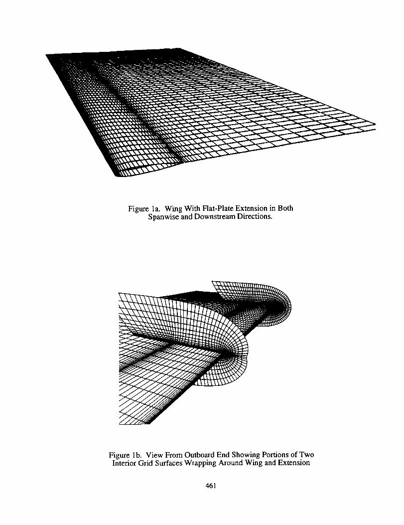
Figure la. Wing With Flat-Plate Extension in BothSpanwise and Downstream Directions.

Figure lb. View From Outboard End Showing Portions of TwoInterior Grid Surfaces Wrapping Around Wing and Extension

461

Figure lc. Close-Upof Grid SurfaceWrappingAroundLeadingEdgeof Flat-PlateExtension

462