N66 3! - NASA · meetings on the subject is the session on "Computers in Network ... W. Mayeda and M. E. Van Valkenberg, "Network Analysis and ... Chapter 26, pp. 280-290

Annual Report on

Computer-Aided Circuit Analysis

Submitted to

;

NATIONAL AERONAUTICS AND SPACE ADMINISTRATION

Office of Grants and Research Contracts

Washington D. C 20546

This work was done under the NASA grantNGR-_-023-0v4, during the period May 15,1965 to May 14, 1966, at the Electrical

Er_neerJng Department, Villanova University,Villanova, Pennsylvania.

GPO pq_(-_

CFST_ p__

$

5

: i :; :: ¸/: ¸¸¸: )': ,:/i̧

N66 3!

{PAGES}

14_l_SA C_ O_ TMX OR AD N_h_ISERI

_ kk _- , .

.... : _.CI C.-•

RE'ARCH-4/qD DEVELOPMENT DI_QSION

XYILLANOVA UNVCERSTi'y

VILLANOVA. pE NNSYLVANn

https://ntrs.nasa.gov/search.jsp?R=19660021934 2018-06-18T03:36:50+00:00Z

Annual Report on

Computer-Aided Circuit Analysis

Submitted to

NATIONAL AERONAUTICS AND SPACE ADMINISTRATION

Office of Grants and Research Contracts

Washington D. C 20546

This work was done under the NASA grantNGR-39-023-004, during the period May 15,1965 to May 14, 1966, at the Electrical

Engineering Department, Villanova University,Villanova, Pennsylvania.

PRINCIPAL INVESTIGATOR

Professor of Elecffrical Engineering

HENRY,. KO_NCEDirector of Re_rch and Development

U

RESEARCH AND DEVELOPMENT DIVISION

VILLANOVA UNIVERSITY

VILLANOVA, PENNSYLVANIA

The contributors to this report are

Tsute Yang

J. J. Hicks

R. M. Jansen

C. P. Rich, Jr.

J. J. Perkowski

Table of Contents

Annual Report of the Research on

Digital Computer-Aided Circuit Analysis

under the NASA Grant NGR-39-023-004

covering period from May 15, 19(_5 to May 14, 1966.

Section

I°

II.

III.

IV.

V.

VI.

VII.

Literature Search

Study of the Available Programs -- ASAP and ECAP

Adaptation of Current Techniques to Moderate Size Computer

On-Line Experience in Time-Sharing Computing Systems

A Note on the Accuracy of Monte Carlo Method

Generation of Random Numbers on IBM 1620 Computer

Future Plans

ERRATA

page

1

28

32

39

41

42

51

55

73

77

78

85

106

107

114

116

line printed as should read

3 catagorie s categories

10 fortet forte

1 Machine Machines

10 j J

2 from bottom C 4 _ C 4

7, 8, 9 L 3 _5 L 3

Fig. 8 L 3 L 3 Q

C4 C 4 Q

1 Caption "Table 1" to be added.

5 Matrix equation to be labelled as (2)

18 10 16

11 1, 2 1, 3 3, 2 3, 3

5, 11 (2) and (4) to be interchanged.

This page is redundant.

19 NPS NBS

11 x x 2

Equation for sigma to be labelled as (2.2).

Section I. Literature Search

One of the initial activities of computer-aided analysis of electric circuits

consisted of a literature search in the subject area. Publications in the professional

and technical journals may be classified into two catagories: those dealing with the

general approach of analyzing circuit performance of any configuration within given

sets of constraints, and those tailored for the design of specific types of networks.

The primary interest of this project has been in the investigation and development

of techniques and programs for the analytic solution of circuit problems in general.

There is evidence of growing interest and activity both in industry and research

institutions in exploiting digital comp_iters as an aid in system design and reliability

evaluation [ 1 ], [ 2 ]. It gradually comes to the realization that progress and

practicality of the concepts involves more than the mathematical model formulation

and digital algorithm applied to circuit solutions. Various other facets such as man-

machine interface, time cost of operation, etc. will influence and contribute signifi-

cantly to the success of the program [ 3 ].

In order to provide the uninitiated with a starting base to get into the area of

computer-aided analysis and design and the specialists in the field with a ready

reference which would reflect the current development in research and industry, a

comprehensive bibliography is attempted and completed with 205 entries as included

in this report. It is expected that the Bibliography will be revised and brought up to

date and distributed when necessary.

One difficulty encountered in the preparation of the Bibliography is to arrive

at a balanced medium between indiscriminative exhaustiveness whichmaytend blurring

the significant contributions, and unintentional or misjudged omissions which would

adversely affect its usefulness as a source of reference. Since the interest of the

research activity weighs heavily on the analysis and design of conventional electronic

circuits, many important titles which may be excellent background literature in the

application of digital computer for circuit analysis are not contained in the Biblio-

graphy. Specific examples include Kron!s method of large system analysis, Monte

Carlo sampling technique in general digital simulation, computer solution of matrix

functions and of nonlinear differential equations, and the design of graphic display as

computer output. Another notable missing segment is concerned with the use of digital

computers in electric power machinery design, power system distribution and trans-

mission. There is a great wealth of literature in that area published in the IEEE

Transactions on Power Apparatus and Systems and during the Power Industry Computer

Application Conferences.

An early effort in analyzing the potentialities of automatic digital computers

to research seems to be the technical paper in six parts by Clippinger, Dimsdale, and

Levin [4] published in the Journal of the Society of Industrial and Applied Mathematics

in 1953-54. Although the possible use of computers in the analysis of electric circuits

has been recognized for some time, the first recorded arrangement in technical

meetings on the subject is the session on "Computers in Network Synthesis" in 1957

WESCON Convention at which time three papers were presented.

T. R. Bashkow and C. A. Desoer, "Digital Computers and Network Theory"

D. T. Bell, "Digital Computers as Tools in Designing Transmission Networks"

W. Mayeda and M. E. Van Valkenberg, "Network Analysis and Synthesis byDigital Computers"

-2-

In 1961 the IRE Transactions on Circuit Theory issued a special number on Network

Design by Computers, including the following papers:

G. M. Cohen and D. Plantnick, "The Design of Transistor IF Usingan IBM 650 Digital Computer"

C. A. Desoer and S. K. Mitra, "Design of Lossy Ladder Filters byDigital Computer"

D. C. Fiedler, "A Combinatorial-Digital Computation of a NetworkParameter"

S. Hellerstein, "Synthesis of All-Pass Delay Equilizers"K. Yamanoto, K. Fujimoto, and H. Watanabe, "Programming

the Minimum Inductance Transformation"

A Computer Program Reviews Department has since been inaugurated to the

Transactions under the editorship of P. R. Geffe, which collects and publishes titles

and reviews of available programs on circuit theory problems. There was a symposium

on the Design of Networks with a Digital Computer at 1962 IRE International Convention

when four papers were presented.

F. H. Branin, Jr., "D-C and Transient Analysis of Networks Usinga Digital Computer"

O. P. Clark, "Design of Transistor Feedback Amplifiers and Automatic

Control Circuits with the Aid of a Digital Computer"C. L. Semmelman, "Experience with a Steepest Decent Computer Program

for Designing Delay Networks"G. C. Temes, "Filter Synthesis Using a Digital Computer"

In 1963 Lockheed Missiles and Space staff prepared an annotated bibliography on

computer-aided analysis and design with 63 entries.

C. M. Pierce, "The Design and Analysis of Electrical and ElectronicSystems by Means of Digital Computers: An AnnotatedBibliography", Lockheed Missiles and Space Co.,September, 1963; SB-63-65; ASTIA Document AD 439 440.

More recently the Third Allerton Conference on Circuit and System Theory, October

20-22, 1965, a special session was devoted to the Network Analysis and Design by

-3-

Digital Computers.

R. M. Golden, "Digital Computer Simulation of CommunicationSystems Using the Block Diagram Computer: BL(_DIB"

J. Katzenelson and L. H. Seitelman, "An Iterative Method forSolution of Nonlinear Resistor Networks"

M. L. Liou, "A Numerical Solution of Linear Time-Invariant

System"

C. Pottle, "On the Partial Fraction Expansion of a RationalFunction with Multiple Poles by Digital Computer"

H. C. So, "Analysis and Design of Linear Networks withVariable Parameters Using On-Line Simulation"

A. D. Waren and L. S. Lasdon, "Practical Filter DesignUsing Mathematical Optimization"

In the following Bibliography the entries are arranged in the alphabetic

order of the last name of the first author of each paper. A subject index and a

chronological index are appended.

Reference s

{1]

[21

[31

[4]

H. S. Scheffler, ed., "Reliability Analysis of Electronic Circuits, "Autonetics Division of North American Aviation Inc., 1964.

University of Michigan Engineering Summer Conference on "Applicationof Computers to Automated Design," 1964 and 1965.

D. T. Ross and J. E. Rodriguez, "Theoretical Foundations for theComputer-Aided Design System, " Proc. Spring JointComputer Conference, AFIPS, vol. 23, pp. 305-322, 1963.

R° F, Clippinger, B. Dimsdale, and J. H. Levin, "Automatic DigitalComputers in Industrial Research," Jour. SIAM,pt. I, vol. 1, pp. 1-15 Sept. 1953pt. H, vol. 1, pp. 91-110 Dec. 1953

pt. HI, vol. 2, pp. 36-56 Mar. 1954pt. IV, vol. 2, pp. 113-131 June 1954pt. V, vol. 2, pp. 184-200 Sept. 1954pt. VI, vol. 3, pp. 80-89 June, 1955

4

A BIBLIOGRAPHY ON DIGITAL COMPUTER-AIDED

CIRCUIT ANALYBIS AND DESIGN

(revised May, 1966)

-5-

(I) M.W. Aarons _nd M.J. Goldberg, "Computer Methods for Integrated

Circuit Design", Electro-Technolo_y, vol. 75, no. 5,pp. 77-81; May, 1965.

(2) M.R. Aaron and J.F. Kaiser, "(_.the Calculation of Transient

_esponse", Proc. IEEE, vol. 53, P. 1269; September,1965.

(3) J._ Abrahmas, "Amplifier Design with a Digital C_mputer",

Electronic _ngrg., vol. 37, pp. 740-745; November, 1965.

(2) G.E. Adams and J.E. Gerngross, "IBM 650 as a Tool for Ana1_sis

of Transmission and Distribution System Problems", Power

Apparatus and Systems, no. 40, (AIEE Trans. vol. 77,

pt. 3) PP. 1236-124L; February, 1959.

(5) _.K. Adams, "Di_ital Computer Analysis of Closed-Loop Systems

Using the humber Series Approach", Applications and

Industry, no. 67, (AIEE Trans. vol. 82, pt. 3) PP. 238-

240; July, 1963.

(6) F.A. Applegate, "Statistical Circuit Analysis Based on Part Test

Data", Electro-Technology, vol. 71, no. 5, p:_. lh0-1_5;May, 1963.

(7) K.G. Ashar, et al. "Transient _nalysis mud Device Characterization

of ACP Circuits", I_ J. _es. and Bey., vol. 7, pp. 207-223; July, 1963.

(6) _.D. Ashcraft and _. F©chwald, "Design by _orst-Case Analysis: a

Systematic _thod to Approach Specified _el_abl/ity

_equirements", IRE Trans. on _eliability and Q-ality

Control, vol. _QC-IO, no. 3, PP. 15-21; November, 1961.

(9) A.G. Atwood and L.C. Drew, "Computer Analysis of au Integrated

Circnit Amplifier", RCA Engineer, vol. lO, no. 3, PP. 27-

29; October/November, 1964.

(lo) W. Austin and K. Angel, "Computer Solutions Aid Rectifier Filter

Design", Electronic Industries, vol. 23, no. 12, pp. 54-57; December, 1964.

H.S. Balaban, "Selected Bibliography on rmliability", L_E Trans.

on Feliability and Quality Control, vol. _QC-11, pp. 86-103; July, 1962.

(12) T.C. Bartee, "Computer Desicn of _Itiple-Output Logical Networks",

IRE Trans. Electronic Computers, vol. EC-IO, pp. 21-30;March, 1961.

-6-

(13) T._. Bashkow snu C.A. Desoer, "Digital Computers and hetwork

Theory", _ESCO_ Co_v. _ecorm, vol. l, pt. 2, pp. 133-

136; 1957.

, , "_<etwork Analysis", Mathematical Methods for DigitalG_ters (book) Chapter 26, pp. 280-290; John a__ley,1960.

(15) W.F. Baur, D.L. Gerlough and J.W. Granholm, "Advanced Computer

Application", IRK Proc. vol. 49, pp. 296-304; January,1961.

(16) J.H. Beaudette and P.A. Honkanen, "PECanS Circuit Analysis ofNonlinear Systems", I_ 7090 Program Writeup, I_

Development Lab., Pougakeepsie, N.Y. 1961.

(IY) F. Hecx, "Harmonic _naiyszs Usxng a Digital Computer", The

Computer J. vol. l, p. /17; October, 1955.

S.D. Bedrosian, "Finding the 1,_rimum Complete Subgraph in

Coding Models for Random Access _ommunications", iE_E

Inuernat'l. Cony. 1_cord, vol. 1h, pp. 250-253; 1966.

D.T. _ell, "Digital Con_u_ers as _ools in _esi_g Transmission

Networks", wE_uN Cony. _e_ora, ,ol i, pt. 2, pp. AAS-

A53: A957.

(20) A.H. Benner and B. _redith, "Designing _eliability into

Electronic Circaits", Proc. Eat'l. Electronics Cor_.,

vDl. i0, pp. 137-ih5; 1954.

(21) C.L. Bertin, "Transmission-Line _esponse Using Frequency

Techniques", IHM J. Res. and Dev. vol. 8, pp. 52-63;

Jm_- m--y, 1964.

(22) H.D. Bic_ley, et al. "Digital Techniques for Voltage Regulation

Studies", Automatic Control, vol. 15, no. 6, pp. 26-30;

December, 1961.

(23) J.A.C. Bingham, "A _ew Method of Solving the Accuracy Problem in

Filter Design", IEEE Trans. on Circuit Theory, vol. CT-11,

pp. 327-341; September, 196h.

_24) G.T. _ird, "On the Basic Concepts o1"Reliability rredlction",

Proc. 7th Nat'l. Syrup. on ._liability and _uality

Control, pp. 51-54; Janmary, 1961.

(25) B. Birtwistle and B.M. Dent, "Digital Computer as an Aid to the

Electrical Design Engineer", The Engineer, vol. 201,

pp. hh0-442; May 4, 1956.

-7-

(26)

C27j

(26)

_29)

t,30)

(31)

(32)

(33)

(35)

(36)

(37)

_. Bongenaar and N.C. de Troye, "_orst-Case Considerations in

Designing Logical Circuits", IEEE Trans. on _._ectronic

_c_zputers, vol. EC-14, pp. 590-599; August, 1965.

A. Brameller _nd J._. Denmead, "Some Improved Methods for uigital

i_etwork Analysis", Proceedings of I._._. vol. 109, Part A,pp. 109-i16; 1962.

r.H. Branin, Jr., "D-C Analysis Portion of PETAP - A Program 1"or

Analyzing Transistor Switching Circuits", IBM fech. Rept.

00.701, I_ Development Lab. Po,,ghkeepsie, t_.Y. 1959.

, "D-C and Transient Analysis of Networks 0slng a

Digital Computer", IRE Cony. Record vol. 10, pt. 2,

pp. 236-256; 19G2.

, "MacrzLne Analysis of hetworks _nd Its Application",IB_I Tech. Rept. TR Ou.855; zarch 30, 1962.

_._. Branin, Jr., "A New Method for Steady-State A-C Analysis of

RLC Networks", IE_E Internat'l. Cony. _ecord vol. 14,

pt. 7, pp. 218-223; 1966.

N.G. Brooks and H.S. Long, "A Program for Computing the Transient

Response of Transistor Switching Circuits-PETAP", IHM Tech.

_ept. 00.700, IHM Development Lab. Pou_Jlkeepsie, N.Y. 1959.

A. Brown, et al, "Mathematical Circuit Analysis and Design",Remington Rand Univac Div. Scientific Rpt. no. 2. AFCRL-

191; March, 1961 ASTIA AD 259786.

H.E. Brown, L.K. Kirchmayer, C.E. Person and G.W. Stagg, "DigitalCalculation of 3-phase Short Circuits by Matrix Method",

Power Apparatus and Systems no. 52, pp. 1277-82 (AIEE

Trans. vol. 79 pt. 3); February, 1961.

_R. Brown, "A Generalized Computer Procedure for the Design of

Optimum Systems", AIEE Trans. Comm. and Electronics vol.78, no. i, pp. 285-293; July, 1959.

J.D. Brule and B.P. Sah, "Time Response Characteristics ofLinear Networks and Transformation Methods in Network

Synthesis", Syracuse Uz_v. l_eport; Aug_ist, 1961;

_9 257 822.

K.J. B_tler and J.N. _arfield, "A Digital Co:mputer Program for

Reducing Logical States to a Minimal Form", Proc. Nat'l.

Electronics Conf. vol. 15, pp. h56-466; 1959.

_8

(39)

(4o)

(20)

._T. Byerly, R._. Long and C._. King, "Logic for Applying

Topological _thods to Electric Networks", Commun. and

E_lectronics, no. 39, (AIEE Trans. vol. 77, pt. l) pp. 657-667; November, 1958.

D.A. Calahan, "I,bdern Network Analysis" (book), vol. i, Chapter 5,Use of the Computer in Appreximaticm. Hayden Book Co.

New York, N.Y. 1964.

, "Computer Generation of Equivalent Networks", IE_EConv. Record, vol. 12, pt. i, pp. 330-337; 196_.

, "Computer Solution of the Network _ealization

Problem", Proc. 2nd Allerton Conf. on Circuit and SystemTheory, pp. 175-195; 1964.

|

, "Cemputer Design of Linear Frequency Selective

Networks", Proc. l_tE vol. 53, PP. 1701-1706;November, 1965.

J.I. C_!eton, N. Ghackan and r._. Martin, "The Use of Automatic

Programming Techniques for Solving _ugineering Problems",Cc_un. and Electronics no. 45, (AIEE Trans. vol. 78,pt. i) pp. 596-601; November 1959.

E.V. Carter, "Thermal Analysis of Integrated Circuits",

Proceedings 2nd Design Aids Symposium, Autc_etics,

Anheim, Calif., Pub. no. 558-A-14, paper no. II;

September, 1963.

L.C. Casady and H.T. Breen, "Transistor and Dioce State Finding

_outine", Proceedings 2nd Design Aids Symposium,

Autonetics, Anheim, Calif., Pub. no. 558-A-14, paper no.V; September, 1963.

P.W. Case, et al. "Solid Logic Design Automation", IBM J. Res.

and Dev. vol. 8, pp. 127-140; April, 1964.

Y.N. Chang and O.M. Georce, "Use of High-Speed Digital Computors

to Study Performance of Complex Switching Networks

Incorporating Time Delays", Ocmmun. and Electronics

no. _6, (AIEE Trans. vol. 78, pt. I), pp. 982-987, 1959.

L-H Shang Cheo, "Arbitrary Delay _qualization Utilizing Digital

Computer IBM 704", Univ. of California Report; July,196L ,PB15o 512.

D.H. Chung and J.A. Palmieri, "Design of ACP Resistor-Coupled

Switching Circuits", IHM J. Hes. and Dev. vol. 7, pp.190-198; July, 1963.

-9-

O.P. Clark, "Desi_nnof Transistor Feedback Amplifiers and

Autcmatic Control Circuits with the _Lia of a DiL__ital

uomp_er", I_ Conventlon Xecord, vol. iO, pt. 2, pp. 22b-235; 1962.

(5.L)C. Clmuies-l_oss and S.S. Husson, "Statistical Techniques ir_

Circuit Optimization", Proc. _iat'l h_ectronics Conf.

vol. 18, pp. 325-334; 1962.

G.H. Cohen and D. Platnick, "The uesign of Transistor IF

Amplifiers Using an I_i 650 Digital Computer", I._ Trans.

Circuit Theory, vol. CT-8 pp. 237-243; September, 1961.

E.U. Cohler, "Statistics Applied to Computer Circuit Design", The

Sylvania Technologist, vol. 12, pp. 134-139; October 1959.

(54) D. Coleman, F. Wstts and _.B. SRipley, "Digital Calculation of

Overhead-T,_ansmission-Line Constants", Power Apparatus and

Systems, no. 40, (ALES Trans. vol. 77, pt. 3), PP. 1266-1268; February, 1959.

(55) D.F. Cooper, "An Integrated Circuit Desi;m for a Hi_ih Speed

Commercial Computer", Solid State Jesign, vol. 6, no. 6,pp. 21-25; October, 1965.

(56) M.S. Corrington, "Simplified Calculation of Transient f_esponse",

Proceedings of IEEE. ,ol. 53, Pp. 2_y-292; March, 1965.

t57) E.L. Cox, "A Compater-_rogra_mned Component Tolerance Analysis",

Diamond Ord. Fuze Labs :report; h_rch 20, 1962, ASTIA AD269 212.

(5@) M.D. Creech, "F_nding the Natural Frequencies of an Undamped

Linear System with a Di_ital Computer", American Society

of _avaA Engineering, pp. 129-132; February, 1962.

(59) D._I. Crosby mud H.d. Kaupp, "Calculated _aveforms for Tunnel

Diode Locked-Pair Circuit", Proc. Eastern Joint Computer

Conf. vol. 18, pp. 233-239; December, 1960.

(60) J.B. Dennis, "_L_themstical Programnin{_ and _lectrical Networks",

(book), John Wiley and Sons 1959.

(61) , _F. Nease and R.M. Saunders, "System Synthesis )_th

Aid of DiStal Computers", Commun. and Electror&cs no. 45,

(AI_ Trans. vol. 78, pt. 1), pp. 512-515; November, 1959.

(62) , "Distributed Solution of _Qetwor_ froramminG Problems",

Proc. First Allerton Conf. on Circuit and System Theory,PP. 367-384; 1963.

- i0 -

(63)

(6n)

(65)

(66)

(67)

(66)

(69)

(70)

tfl)

(72)

(73J

(7h#

C.A. Desoer and S.K. Mitra, "Desi_on ol Lossy _adder Filters by

Digital Computer", I_ Trans. _ircuit Ineory, vol. OT-8,pp. 192-201; September, 1961.

A.J. DeVilbiss, D.j. Spencer and G._. Hogsett, "A Norst-Case

Circuit Design Technique Utilizing a Small Digital

Computer", Jet Propulsion Laboratory, California

Institute of Technology, Pasadena, California; October,±964.

G. Dxaz, "Computer Methods for Analyzing Test Data", Electro-

Technolo_ voA. 71, no. 5, pp. 152-155; M_y, 1963.

R.J. Domenico, "Simnlation of Transistor Switching Circuits on

IBM 704", IRE Trans. on Electronic Computers, vol. EC-6,pp. 242-247; December, 1957.

_4.H. Doxtator and F. Arnold, "PRESS: An IH_ 704 Program for

Performance and ._eliability Evaluation by Synthetic

Sampling", Tech. Rept. ul.Ol.ll2.602, IHM, _dicott,h. Y.; December, 1959.

L.C. Drew and A.G. Atwood, "Using the _omputer for Integrated

Circuit Analysis", Electronic Industries vol. 23, no. 7,Pp. 52-57; July, 1964.

T.E. Duby, "Linear Circuit Analysis Using the SPADE Program",

Proceedings 2nd Design Aids Symposium, Antonetics,

Anaheim, Calif. Pub. no. 558-A-i4, paper no. I:September, 1963.

W.J. Dunnet and X.C. no, "Statistical Analysis of Transistor-

Resistor Logic Networks", I_ Cony. Record, vol. 8, pt. 2,pp. ll-hO; 1960.

A.n. El-Abiad, "Digital Calculation of Line-to-Grc_nC Snort Cir-

cuits by Matrix Method", Power Apparatus and Systems no.48, tAIEE Trans. vol. 79, pt. 3)PP. 323-332; June, 1960.

P_ _idone ant G._. Stagg, "ua_cu±ation of Short

Circuits Using the High-Speed DXgital Computer", Power

App. ana Systems no. 51, (AI_E Trans. vol. bO, pt. 3#,

Pp. 702-708; December, 1961.

, "Digital Computer analysis of Large Linear Systems",

_roe. First Allerton _on__. on Circuit and System Theory,pp. 205-220, 1963.

Electro-Technology Staff Report, "The Computer as a Design Tool -

The M.i.T. Approach", Elec_ro-Technology, vol. 72, no. 5,pp. 112-115, pp. 119; Novenmer, 196_.

- 11 -

(75)

(76)

(77)

(79)

(80)

_81)

(82)

(03)

(85)

(86)

L._i. Fairbrother ,%haH.u. Bassett, "uomputer Program 1"or

Analysing l,,et_orkscontainlng i%ree-terminal _ctive

_evxces characterizeo by their Awo-p_t Par_meters",

The Raa_o anm _lectronlc _gineer, vol. 29, pp. 05-92;FeDruary, A965.

H. Falk, "The Computer as a Design Tool", Electro-Technology,

vol. 72, no. 7, pp. 48-50; July, 1963.

, "Comouter Programs for Circuit Design", Electro-

Technology, vol. 73, no. 3, PP. lOl-104, pp. 162,164;March, 1964.

J.V. Fall, "A Digital Computer _rogram for the Uesign of Phase

Correctors", IRE Trans. Oircuit Theory, vol. OT-8,

pp. 223-236; September, 1961.

, "Digital Computer Analysis of lhree-Terminal Two-Port

Networks", Proc. Inst. Radio Electronics Engrs., Australia;vol. 26, pp. 167-T3; May, 1965.

Ferguson, "Application of Digital C_uputer Techniques to Power

System Analysis", Proc. First P_dwest Syrup. on Circuit

An alysis, pp. IL-1 to 14-9; 1955.

R.W. Ferguson, R.W. Long an_ L.J. i_hudt, "Digital Calculation of

Network Functions Osed in _oss Formula StuCies", Commun.

and _lectronics, no. 39, (alEE Trsns. vol. 77, pt. 1),pp. 64T-652, November, 1958.

D.O. Fiedler, "A Combinatorial-Digital Computation of a Network

Parameter", IRE Trans. Circuit Theory, vol. CT-6,

pp. 202-209; September, 1961.

T. Fleetwood, "Automauic Solution of Network Frequency _esponse",

Electronlc Engrg. vol. 3f, PP. bl2-61_; September, 196b.

D.A. Franks, "A New Automatic Method _or the Desi_a of Low

Voltage Transformers on IB_ 704", I_E Cony. Record,vol. _, pt. b, pp. 193-204; 1960.

W.D. Fryer and W.C. Schultz, "Digital Simulation of Transfer

Functions", Froc. Nat'l Electronics Conf. vol. 17,pp. 419-420; 1901.

T. FuJisawa, "Op_imlzation of Low-Pass Attenuation Characteristics

by a Digital Computer", Proc. 6th Midwest Symp. on CircuitTheory, pp. PI-PI3, 1963.

12 -

(87) P.K. Geffe, "Predistorted Fxlter Design with a Digital _cEputer u,

_ESCON _ecord, vol. 2, pt. 2, pp. 10-22; 1958.

(88) , "Computer Program Reviews", IRE Trans. on CircuitTheory, CT-9 p. 307; September, 1962

CT-±I p. 512; December, 196_

CT-12 p. 3Oli June, 1965.

(89; M. _idberg, =Network Analysis by Ccaputer", Instnments and

Control Systems, re1. 38, pp. 175-I[8; September, 1965.

(90) _a. Golden, "Digital Computer Simulation of Communication Systems

Using the Block Diagram Ccmpater: B_IB", Prec. of 3rd

Allerton Conf. on Circuit System Theory, pp. 690-707;

October, 1965.

_91) G.H. Goldstick and D.G. Hackle, "Design of Computer Circuits

Using Linear Programming Techniqaes", I_ Cony. Record,

vol. 9, pt. 2, pp. 224-240; 1961; also IRE Trans. on

Electronic Computers, vol. EC-11, pp. 518-530; A_gust,1962.

(92)

(93)

_G. Goodman and R.L. Cummins, "Computer Determination of

Iscmorpaisms in Linear Graphs", Proc. 8th _Ldwest Syrup.

on Circuit Theory pp. i2-1 to 12-12; June, 1965.

B.J. Grinnell, "Analysis Testing for Improved Gircuit

Reliability", Proc. 6th _at'l. Syrup. on Reliabilityand Quality Control, pp. 103-108; 19G2.

P.P. Gupta and M.W.H. Davies, "Digital Computers in Power System

Analysis", Proc. fuss. Elec. _ngrs. (London) vol. 108,

part A, pp. 383-404; October, 1961.

(95) T.J.b. Hannom and G. Kaskey, "Digital Uomputer as a Design Tool",

IRE Cony. Record. vol. 13, pt. 6, pp. 27-38; 1965.

(96) J.N. Hatfield, "A Linear Circait Analysis Program for the IHK

1620/131A 2Ok Data Processing System (CIRCS)", Jet

Propulsion Lab. Pasadena, Calif.; F_y, l_Gh.

(97; P_K. Maynes, "Transient Analysis of GryotAon Networks by Computer

Simnlatlc_", Proc. IRE, vol. 49, pp. 2h5-257; January, 1961.

(98) C.L. Hege_s, .TRL Circuit Design Implemented by Gomputer",Electronic Design vol. 12, pp. 40-46; March 16, 196_.

(99; L. Hellerman, "Monte Carlo Analysis and Design Program", I_

Technical Note, TNOO.IIOOO.Sh.

- 13 -

(I00)

(ioi)

(1o2)

(i03)

(lOb)

(io5)

(ioo)

(io7)

tlob)

(lO9)

(iio)

(lllj

ano M.P. xacite, "Reliability Techniques for

h_ectronic Circuit Design", IRE Trans. on Reliability

and Quality Control vol. HQC-I_, pp. 9-16; September,1958.

, "A Computer Application to Reliable Circuit Design",

IRE Trans. Reliability and Quality Control vol. H_G-II,pp. 9-18; May, 1962.

anc E.J. Skiko, "Methods of Analysis of Circuit

Transient Performsnce", IBM J. _es. anO Dev. vol. 5,

PP. 33-_3; January, 1961.

S. Hellerstein, "Synthesis of All-Pass _elay Equilizers", IRE

Trans. on Circuit Theory, vol. CT-8, pp. 215-222; September,1961.

_H. Hindricks, "A Statistical _ethod for Analyzing the Performance

Variation of Electronic Circuits", Convair Report no. ZX-7-

009; October, 1953.

, "A Second Statistical Method for Analyzing the

Performance Variation of Electronic Circuits", Convair

Report No. AZ-7-OIO0; February, 1956.

W. Hochwald and N.D. Ashcraft, "Jesigm by Worst-Case Analysis",

IRE Trans. on Reliability mud Quality Control; November,1961.

J.L. Hogin, "An Active L_-Pass RC Filter Configuration Utilizing

the Voltage Follower", Proc. 7th RiCwest Syrup. on CircuitTheory, pp. 179-191; 1964.

K.H. Hosking, B.M._. havanaugh and M. Sadler, "The Application of

'Deuce, to the Analysis of Linear Passive Networks",

l._oni Rev. vol. 25, no. 2, pp. 139-I_6; 1962.

T. ledoroko, T. Tsacniya and H. Wat_nabe, "A New Calculation

Method for the Design of Filters by Digital Computer with

the Special Consideration ol the Accuracy Problem", I_EE

Cony. Record, vol. ii, pt. 2, pp. 1OO-113; 1963.

International Business _achines Corp., "ib20 Electronic Circuit

Analysis Program (_CAP 1620-_-02A)", IBM, Tech. Publ.

Dept., _nite _lains, N.I.; /805 •

., "ASAP, An Automated Statistical Analysis Program ",

Tech. Rept. prepared for Goddard Space Flight Center,

Greenbelt, _d., Contract no. NAS 5-3373.

- 14 -

(ll2) M.N. John, "A General Method of Digital Network Analysis

Particularly Suitable for Use with Low-Speed Cumputers",

Proc. Inst. Elec. Engrs. (Lencon) vol. 108, part A,

pp. 369-382; October, 1961.

(113) H.J. Joyal, "Power-Supply Circuit Design by DiStal Cumputer

Method", Electrical Mfg. vol. 65, pp. 171-177; May, 1960.

G. Kss_ey, N.S. Prywes and H. Luko_f, "Applications of ComputerstO Circuit Design for UNIVAC LAHC", Proc. wJCC, Los

Angeles, Calif. vol. 19, pp. 185-205; May, 1961.

(115; J. Katzenelscn and L.H. Seitelman, "An Iterative Me_od for

Solution of Nonlinear Resistor Networks", Proc. of 3rd

Allerton Conf. on Circuit and System Theory; pp. 6_7-

658; October, 1965.

(116) T.A. Keenan, u.H. Corm and u. Platnick, "Circuit Study Using

Computer Techniques", Rochester University, Final

Rept. 74 p.; July 15, 1959. ASTIA AD2298_20TS Pm57-593.

(117) J.B. _idc, T.E. edgertc_ and C.F. Ghen, "Transfer FunctionSynthesis in the Time Domain--An Extension of Levy's

Nethod", IEEE Trans. on Education, vol. E-8, pp. 62-

67; June-September, 1965.

(118) W.H. Kin, etal., "On Interative Factorization in NetworkAnalysis by Digital Computer", PToc. EJCC, vol. 18,

pp. 241-253; December, 1960.

(119) E.G. Kimme and F.F. Kuo, "Synthesis of Optimsl Filters for aFeedback Quantization oystem", IEEE Trans. on Circuit

Theory, vol. CT-lO, pp. h05-413; Septenber, 1963.

(120j S. Klapp, "Empirical Parameter Variation Analysis for Electronic

Circuits", IEEE Trans. c_ Reliability and Quality Ccntroi,

vol. RQC-13, pp. 3_-40; March, 1964.

(121) T.B. Knapp, "An Application of Nonlinear Programming to

_muatched Filters", IEEE Trans. on Circuit Theory,

vol. CT-12, pp. 185-193; June, 1965.

(122) F.F. Kuo, _etwork Analysis by Digital Computer", Proc. IEEE,

vol. 55; June, 1966.

(]-23) , "Computer Techniques in Circuit Analysis", A_etworkAnalysis and Synthesis (book), 2nd edition, pp. 438-460;

John Wiley, 1906.

(z2&) and J.F. Kaiser, "System Analysis by Digital Computer",

(book) John Wiley, 1966.

- 15 -

(125)

(126)

(127)

C. hurth, "Analysis of Diode Modulators Having Frequency-Selective

Terminations Using Computers", Electrical C_mmunicatic_,

vol. 39, no. 3, PP. 369-378; 1964.

D.M. Larson and B.J. Grinell, "A Comparison of Methods of Drift

Reliability Determination", Proc. 7th Nat'l. Syrup. cn

Reliability anm Quality Control, pp. 4_8-_5h; 1961.

G.L. Lasher and J.C. Morgan, "A General Method of Predicting the

Transient Response of a Nonlinear Circuit", IHM ResearchRept. RC-7; 1957.

(128) A.P. Lechler, D.C. Mark and H.S. Scheffler, mApp_g Statistical

Techniques to the Analysis of "_lectronic Networks", Proc.

1962 Nat'l Aerospace Electror_cs Conf. pp. A68-172.

(129) G.H. Leichner, "Network Synthesis Using a Digital Computer", Proc.N.y.C. vol. 12, pp. t_30-83o; 1956.

(13o) , "Desi_ing Co_puter circuits w_th a Computer a, J.

Assoc. Computing Much., vol. h, pp. 143-147; April,1957.

(131) B.J. Leon an_ C.A. Bean, "Anal_sis ant Desi_n of Parametric

amplifiers with the Aid of a 709 Computer", IRE Trans.

on Circuit Theory_ vol. CT-O, pp. 210-215; September,1961.

(132) V.S. Levadi, "Simplified Method of Determining Transient Response

from Frequency Response of Linear Networks ant Systems m,

_R_ Gonv. aecoru, vol. 7, pt. 4, PP. 57-68; 1959.

(133)

(134)

(135)

(136)

(137)

J.l. Levin, "Failure Prevention Through Design Optimization

Utilizing Monte Carlo Simnlatic_ Techniques", Solid

State Desi_, vol. 6, no. iO, pp. 26-29; October, 1965.

R.W. Levinge, "A Transfer Function Computer", Electronic Engrg.,

vol. 37, pp. 218-224; April, 1965.

I.C. Liggett, "Examples of Engineering Applications on I_4

Digital Computers", Electrical Engrg., vol. 74, pp. 233-

236; March, 1955.

M.L. Liou, "Numerical Techniques of Fourier Transforms with

Applications", Proc. 2nd Allerton Conf. on Circuit and

System Theory, pp. i14-I_; 1964.

, "A Numerical Solution of Linear Time-Invariant

System u, Proc. of 3rd Allerton Conf. on Circuit and

System Theory, pp. 669-676; October, 1965.

16 -

138) "A Novel Method of Evaluating Transient Response",Proc. IEEB vol. 54, pp. 20-23; January, 1966.

(139) A.J. McElroy and K.M. Porter, "Digital Co_puter Calculation of

Transients in _:lectrical Networks", Power Apparatus and

Systems, no. 59, (AIEE Trans. vol. 82, pt. 3), PP- 88-96;

April, 1963.

(14o) F.J. _cWillisms, "Topological Networa Analysis as a Computer

ATogram"_ I.%E Trans. on Circuit Theory, vol. CT-6,

pp. 135-136; March, 1959.

A.F. D_mberg, F.L. Cornwell and F.N. Hofer, "NET-I Network

Analysis Program, 7090/94 version", Report no. LA-3119,

Los Alamos _cientlfic Laboratory, August, /364.

R.A. Mammano, K.D. Pope _nd E.P. Schneider, "Computer-AssistedCircuit Analysis", E_N vol. lO, no. 14, pp. 132-139;

Nove_ber, 1965.

C 3) J. Marini and _T. Williams, "The _valuation and Prediction of

Circuit PerXormance by Statistical Techniques", Proc.

Joint 14ilitary-lndustry Symp. on Guided Missile

Reliability; 1957.

(144) D.G. Mark and L.H. Stamber, "Variability Analysis", Electro-

Technology, vol. 76, no. I, pp. 37-48; July, 1965.

Q145; W. Mayeaa and M.E. Van Valkanburg, "Network Analysis _nd

Synthesis by Digital G_mputers", WESCON Cony. Record,

vol. I, pt. 2, pp. 137-141_; 1957.

, "Analysis of Nonreciprocal Networks by Digital

Computer", IRE Cony. Record, vol. 6, no. 2, pp. 70-75;195b.

C.S. zeyer, "A Digital Computer Fapresentati_ of the LinearConstant-Parameter Electronic _etwork", _l.I.T.,

Cambridge, Mass., Tech. Mayo 8h36-TM-3, p. II0; August,

1960, ASTIA AD 2J48h37. COTS FB 155h08).

(I 8) _S. Miles, "Transient Response _singMatrizant Procedares",Proceedings 2nd Design Aids _y_posium, Autonetics, Anheim,

Calif., Pub. no. 558-A-14, paper no. IV; September, 1963.

QI49j a.l.T. _es. Lab. Electronics, "Circuit Simulation on a Digital

Computer", Quarterly Progress Report _61; December, 1960 -

February, 19bl.

- 17 -

(150) _.F. Morris and T.E. _ohen, "Autom_tlc Implementation of Computer

Logic", Co_un. ACM, vol. i, no. 5, Pp. 14-30; May, 195b.

(151) F. Moskowitz, "The Analysis of Redundancy Networks", CcmmAn. andElectronics, no. 39, (AIEE Trans. vol. 77, pt. I_, pp.

627-632; November, 1958.

(152) W.F. Niesen, "System Analys_s Using Digital Computers", Electronic

Industries, vol, 19, no. 8, pp. 212-13; August, 1960.

(z53) E. Nussbaum, E.A. Irland and C.E. Young, "Statistical Analysis of

Logic Ulrc_it Performance in Digital Systems", Prec. IRE

vol. 49, pp. 236-244; January, 1961.

(154) E.A. Pacello, "The Use of 'Deuce' _or _etwork Analysis", The

Marconi Review, vol. 2h, no. 142, T_ird Quarter; 1961.

(155) K.C. Patton and U.A. Newey, "Power-System Design - _ew

Techniques", J. Science and Technology, vol. 29, no. I,

pp. 9-19; 1962.

(156) G.M. Pierce, "The Design and Analysis of Electrical, Electronic

Systems by Means of Digital Computers, An AnnotateC

Bibliography", Lockheed Missiles and _pace; September,

1963, p. 3h, An 239

157J S.C. Plumb, "A Program for Statistical Reliability Evaluation

by Synthetic Sampling (STRESS;", Tech. P_bl. no.TR 00.83_, IBM Po-gh_eepsie, N.Y.; January, 1962.

(158; C. Pottle, "On the Partial Fraction _xpansion of a Rational

Function with Multiple Poles by Digital Computer",

IEEE Trans. on uircuit Theory, vol. CT-II, pp. 161-162;

March, 1964.

(159) , "Comprehensive Active Networ_ Analysis by Digital

Computer - A State-Space Approach", Proc. of 3rdAllerton C_nf. on Circuit and System Theory, pp. 659-

676; October, 1965.

(160) M.B. Reed and others, "A Digital Approach to Power-System

Engineering", (in 4 parts;, Power Apparatus and Systems,no. 48 (AIEE Trans. vol. 79, pt. 3)PP- 198-225; June,

1961.

(161; Remington Rana Univac Division, "Mathematical Circuit Analysisand Design", Remington Rand; February 29, 1960, 40 pp.,

OrS PB I_8222.

- 18 -

(162)

(163)

(164)

(165)

(166)

(167)

(16 )

(169)

(17o)

(171J

(z72)

A.L.._iemenschneider and C._. Cox, "DiGital Computer Analysis of

the Tunnel Diode Relaxation Oscillator", _lectronic

Engineering, vol. 36, pp. 382-385; 196h.

D. Rigney, L. _raus and H. Malamnd, "Synthesis of C_rrent

_ave/orms by Type C. Networks", Republic Aviation Report;

August, 1961, PB 155 213.

L.G. Roberts, "Circuit Simalation on a Digital Computer", M.I.T.

Cambridge, _ss., Quarterly Pro_;ress Report, no. bl, pp.

239-251; April, 1961.

L.P.A. J_bichauo, M. Bolsvert and J. Robert, "Signal Flow Graphs

and Applications", (book)_ C_apter 7 "Algebraic Neduction

of Flow Graphs _sing a Digital Computer", pp. 181-195;Prentice-Hall, 1962.

C.W. _osenthal _.nnoH. Simon, "Computers as an Aid in the

Development of T_smission Circuits", Proc. 2nd Allerton

Conf. on Circuit and System lheory, pp. 337-365; 1964.

D.T. Ross and J.E. Hodrigaez, "Theoretical Foundations for the

Computer-Aided Design System", Proc. 1963 Spring JointComputer Gonf. pp. 305-322.

N.A. _outledge, "Logic on Electronic Computers: A PracticalMethod _rReducing Expressions to Conjunctive Normal

Form., Proc. Camb. Phil. Soc., vol. 52, pp. 161-173;

April, 1956.

H. _ston and J. Bordogna, "Electric Networks: Functions,

Filters, Analysis", (book), Section 6-4 "Analysis with

a Digital Computer", pp. 435-445; McGraw-Hill Book Co.,1966.

N. Sato, "Digital Calculation of Network Inverse and Mesh

Transformation Matrices", Power Apparatus and Systems,no. 50 (AIEE Trans. vol. 79, pt. 3), PP. 719-726,°_"October, 1960.

H.S. Scheffler and F.R. Terry, "Description and Comparison of

Five Computer Methods of Circuit Analysis", Prec. 6th

Symposium on Ballistic Missiles and Aerospace Technology,

Los Angeles, 1961, Ed. by C.T. Morrow, L.D. Ely andM.R. Smith, Academic Press, 1961.

, J.J. Duffy and B.C. Spradlin, "MANDE_-A_orst-Case

Circuit Ana_Tsis Computer Program", Proc. 1962 Nat'l

Aerospsce Electronics Conf. pp. 38-53.

- 19 -

173)

(17h)

( 75)

(176)

(z77)

(17o)

(179)

(18o)

( 81)

(i 2)

(183)

J.D. Schoeffler, "The Synthesis of Minimum Sensitivity Networks",

IEEE Trans. on Circuit Theory, vol. CT-II, pp. 271-276;June, 1964.

H. Schorr, "Computer-Aided Digital System Design and Analysis

Using a Register Transfer Language", IEEE Trans. on

Electronic Computers, vol. EC-13, pp. 730-737; December,1964.

L.S. Schwartz, "Statistical Methods in the Design and Development

of Electronic Systems", Proc. I_, vol. 36, pp. 662-670;May, 19h8.

C.L. Se_uelman, "Experience with a Steepest Decent Computer

Program 1or Designing Delay Networks", IHE Cony. Record,vol. 10, pt. 2, pp. 206-210; 1962.

L. Shalla, "Automntic Analysis of £1ectronic Digital Circuits

Using List Processing", Communications ACM, vol. 9,pp. 372-380; May, 1966.

Y. Shiger, T. Takebe, T. Shinozaki, K. Kimara and S. Watanabe,

"Network Design by the Taylor Series Method", Rev. Elect.

Commun. Lab. (Japan) vol. IO, no. 9-10, pp. 483-500;

September- October, 1962.

R.B. Shipley, D. Coleman and C.F. Watts, "Transformer Circuits

for Digital Studies", Power Apparatus and Systems, no. 6_

(AIEE Trans. vol. 81, pt. 3) pp. 1028-1031; February,1963.

J._. Skwirzynski, "The Use of Digital Computers for Network

Analysis", Marconi Rev., vol. 28, no. 158, pp. 195-210;1965.

B.R. Smith and G.C. Tames, "An Iterative Approximation Procedure

for Autcmatic Filter Synthesis", IEEE Trans. on Circuit

Theory, vol. CT-12, pp. 107-112; March, 1965.

H.C. So, "Analysis and DesiL_ of Linear Networks with Variable

Par_eters Using On-Line Simulation", Proc. of 3rd

Allerton Conf. on Circuit anO System Theory; pp. 634-646;

October, 1965.

L.H. Stember, H.S. Scheffler and J.J. Dully, "Circuit Analysis

Techniques Utilizing Digital C_uters", Proc. 7th Nat'l

Syrup. on Reliability and Quality Control, pp. 361-374;1961.

- 20 -

(164)

(187)

(158)

(189)

(Lgo)

(191)

(192)

(193)

(195)

C.W. Stempin, "Application of Matrizant Operators for General

Network Response", Proce_din6s 2nd Design Aids

Symposium, Autonetics, Anheim, Calif., no. 558-A-14,

paper no. Ill; September, 1963.

R.W. Stineman, "Digital Time-Domain Analysis of Systems withWidely Separated Poles", J. of Assoc. C_mputing

Machinery, vol. 12, pp. 286-293; April, 1965.

G. Szeutirmai, "Theoretical Basis of a Digital Compater Prograu

Package for Filter Synthesis", Prec. ist allerton Conf.cm Circuit and System Theory, pp. 37-49; 1963.

N.H. Taylor, "Designing for _eliability", Proc. I_ vol. 25,

pp. 811-822; June, 1957.

G.C. Temes, "Filter Synthesis using a Digital Computer", IRE

Ccnv. Record, vol. I0, pt. 2, pp. 211-227; 1962.

A.O. Thomas, "Calculation of i°rausmission-Line Impedance by

Digital Computer", Power Apparatus and Systems, no. 40

(AIEE Trans. vol. 77, pt_ 3) PP. 1270-1274; February,

1959.

J.B. To_erdahl, A.C. Nelson and K.K. Mazuy, "Mathematical Modelsfor Predicting Pulse Characteristics in Digital Logic

Systems", IEEE Trans. on Electronic Computers, vol. EC-13,

pp. 705-710; December, 1964.

and A.C. Nelson, "Switching Circuit Transient

"_erformance Prediction Using Kmpirical Mathematical

Modeling Techniques", IEEE T_ans. on Reliability and

Quality Control, vol. RQC-I_, pp. 5-14; March, 1965.

J.G. Truxal, "_umericsl Ana_sis for Eetwork Design", IRE Trans.

on Circuit Theory, vol. CT-I, no. 3, PP- 49-60;

September, 1954.

C.G. Veinott, "Electric Machinery Design by Digital Comp_er -

After Nine Years", Elect. Engrg. vol. 82, pp. 275-280;

April, 1963.

S.Y. Wong and M. Kochen, "Automatic _etwork Analysis with a

Digital Computation System", Comm. and Electronics,no. 24 (AIEE Trans. vol. 75, pt. I), pp. 172-175;

May, 1956.

A.D. Waren an_ L.S. Lasdon, "Practicsl Filter Design Using

Mathematical Optimization", Prcc. of 3rd Allerton Conf.

on Circuit and System Theory; pp. 677-689; October, 1965.

- 21 -

(196)

(197)

(198)

(200)

(2u1)

(202)

(2o3)

(2o4)

(2o )

11. gatanabej "A Computational Method for Network Topolo_y",

Trans. cm Circuit T_eory, vol. CT-7, pp. 296-302;

September, 1960.

_.J. gest and H.S. Scheffler, "Design CcmsiCerations for _eliable

Electronic Equipment", Pub. no. 558-A-2, Autonetics;

October, 1962.

D. Wildfeuer, "The Use of Automatic Digital Computation Machine

in Design of Miniature Pulse Transformers and Power

Transformers", Prec. Nat'l Electronics Conf. vol. 16,

pp. 631-651; 1960.

S.B. _illi_ms, P.A. Abetti and E.F. Magnusson, "How Digital

Computers Aid Transformer Designers", General Electric

_ev., vol. 58, pp. 24-25; May, 1955.

and H.J. Mason, "Complete Deslgn of Power Transformers

with a Large Size Digital Computer", Power Apparatus and

Systems, no. 34, (AIF_ Trans. vol. 77, pt. 3), PP. 1282-

1291; February, 1958.

H.M. _all, "Using a Computer for Circuit Analysis", Electronics,

vol. 2, PP. 56-61; November 2, 1964.

B.A.M. Willcox and R.C.V. Macario, "Iterative Procedure for

Analyzing Certain Network by Digital Computer", Proc.Inst. Elect. _grs. (London) vol. 112, pp. 2243-53;

December, 1965.

J.L. __rth, "The Design and Analysis of Electronic Circuits by

Digital C_ters", _eport no. SC-H_64-1355, Sandia Corp.,

October, 1964.

K. Yamanoto, K. FuJimoto and H: _atanabe, "Programming theMinimum Inductance Transformation", IRE Trans. Circuit

Theory, vol. CT-3 pp. 184-191; September, 1961.

G._. Zorbist and G.V. Lago, "Digital Computer Analysis of Passive

Networks Using Topological Formulas", Proc. 2nd Aller_

Conf. on Circuit and System Theory, pp. 573-595; 1964.

22 -

SUBJECT INO_

Amplifiers

Analysis

Bibliography

Books

Computer Programs

Design and

Synthesis

Filters

IntegratedCircuits

3

5

22

7_

112

159

182

2o3

ll

16

1].O

2

33

49

87

117

163

i_2

I0

1

9

6

27

57

79

zi5

z_2

161

183

204

156

39

2_

3

35

55

Pl

119

166

23

186

P

5o

7

-28

_8

81

116

162

164

60

32

I0

36

61

9_

129

167

188

63

188

m_

52

8

29

59

82

_6

169

165

_3

67

157

12

3P

63

io3

130

173

192

87

195

55

--23 -

131

in

30

62

83

120

in7

17o

19o

124

6_

19

40

6_

io6

131

176

195

io7

68

16

33

65

89

122

151

174

19n

_65

77

2O

nl

74

Io9

133

176

lop

17

3n

6p

102

123

152

177

201

169

68

23

_2

?B

113

n6

178

119

21

4o

73

108

:].2_

180

202

86

181

12"I

Ladder Network

Logical l_etwork

Nonlinear Net_ork

14_rical Method

Power Network

aezi_illty

Simulation

Statistical

Technique

Survey

TopologicalMethod

Transfer Function

Transformer

Transients

transistor

Worst-Case

63

12

16

5

4

].69

ii

126

66

6

128

13

].8

ZS_

26

39

54

2O

z_

85

5].

].33

z5

113.

38

37

127

136

71

24

90

_3

z43

25

193

82

_6

137

72

67

97

70

43

92

]32

80

93

197

99

z53

76

z_o

85 zz? _34 ZS_

84 179 198 199 20o

2 7 29 32 36

_27 z32 z38 :39 z_8

28 45 49 52 59 98

8 26 64 i06 i72

70

9_

I00

z6b

zob

95

2oh

56

191

162

15o

z55

i01

182

io5

122

196

9?

168

150

120

ILl

135

2o5

142

102

- 24 -

__ 175

20 192

___ 80 _35 ].99

25 105 129 168 194

13 19 66 127 130 143 I/6 187

17 38 81 e7 lO0 156 150 151

2OO

___ _ 28 32 35 37 h3 _? 53

5_ 6o 6]. 67 116 132 _ 189

_ 59 7o 71 84 _3 _ _7

152 161 170 196 198

1961 8 12 15 16 22 2!_ 33 .3_

36 _.8 52 63 72 78 82 85

94 97 lO2 lO3 lO6 112 114 126

131 _ 153 154 160 163 164 171

183 204

196..../2 11 27 29 30 _;o 5z 57 58

88 91 93 101 108 128 155 157

165 172 176 178 188 197

1963 5 6 7 44 45 49 62 65

69 73 74 76 86 109 iii 119

139 lh8 156 167 179 184 186 193

- 25 -

9

iz5

190

I

79

115

159

18

i0

68

136

201

2

83

117

18o

31

21

77

inz

203

3

88

121

181

122

23

8_

158

so5

26

89

133

182

123

39

96

Z62

_m

90

134

185

zs&

no

98

166

55

92

137

191

138

zo7

173

56

95

142

195

z69

46

120

17h

75

ii0

z_

202

177

- 9.6 -

Section II. Study of the Available Programs -- ASAP and ECAP

Three existing digital computer programs written expressly for circuit

analysis and evaluation were reviewed and examined, namely, the Automated

Statistical Analysis Program (ASAP) [1], the Circuit Analysis System (CIRCS}

[2 ], and the Electronic Circuit Analysis Program ( ECAP ) [ 3 ] ; the first and the

third being developed by the International Business Machines GorpQ_atio_,:a_l_

second at the Jet Propulsion Laboratory. They may be regarded as the offspring

of the same lineage, because they share the same philosophy of attacking the problem

and they possess strong similarities in modeling and formating. All three programs

have the capability of accepting a topological description of the circuit in simple

language, writing the circuit equations according to Kirchhoff's current law, and

carrying out" the analysis requested.

The ASAP is primarily designed to perform a Monte Carlo statistical

analysis on the d-c currents and voltages of circuits containing transistors and

diodes. It computes two types of sensitivities. The first type is a qualitative

analysis where the measure of the spread of each parameter about the mean value

is taken into consideration. The second type is based on a one per cent deviation of

each component parameter from its nominal value. The CIRCS program provides

options of d-c, a-c, and transient analysis, and also the Mandex worst case and

sensitivity calculations. The ECAP, which has recently been released to general

public, has the additional feature of including mutual inductance as a circuit element

without finding its equivalent tee or pi. The ASAP works on the IBM-7090/94

computer while the other two operate on IBM-1620 with a 1311 disk file system.

- 27 -

CIRCS requires a 20k core storage unit while ECAP requires a 40k core storage.

Because ECAP is inclusive of the features of CIRCS, discussions and observations

will be made in the this section of the report with regard to ASAP and ECAP only.

One of the justifications in using the digital computer for circuit analysis

and design is to obtain information concerning the circuit operation and performance

which would otherwise be unobtainable by other means, either for physical reasons

or for time considerations. For instance, in the reliability study of a circuit com-

prising many component parts, it is practically impossible to find out systematically

all the effects on the output of varying each component to a different extent on a lab

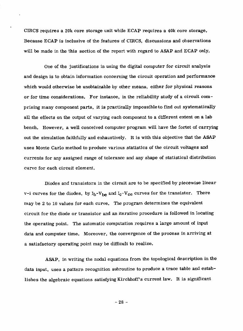
bench. However, a well conceived computer program will have the fortet of carrying

out the simulation faithfully and exhaustively. It is with this objective that the ASAP

uses Monte Carlo method to produce various statistics of the circuit voltages and

currents for any assigned range of tolerance and any shape of statistical distribution

curve for each circuit element.

Diodes and transistors in the circuit are to be specified by piecewise linear

v-i curves for the diodes, by Ib-Vbe and Ic-Vce curves for the transistor. There

may be 2 to 10 values for each curve. The program determines the equivalent

circuit for the diode or transistor and an iterative procedure is followed in locating

the operating point. The automatic computation requires a large amount of input

data and computer time. Moreover, the convergence of the process in arriving at

a satisfactory operating point may be difficult to realize.

ASAP, in writing the nodal equations from the topological description in the

data input, uses a pattern recognition subroutine to produce a trace table and estab-

lishes the algebraic equations satisfying Kirchhoff's current law. It is significant

- 28 -

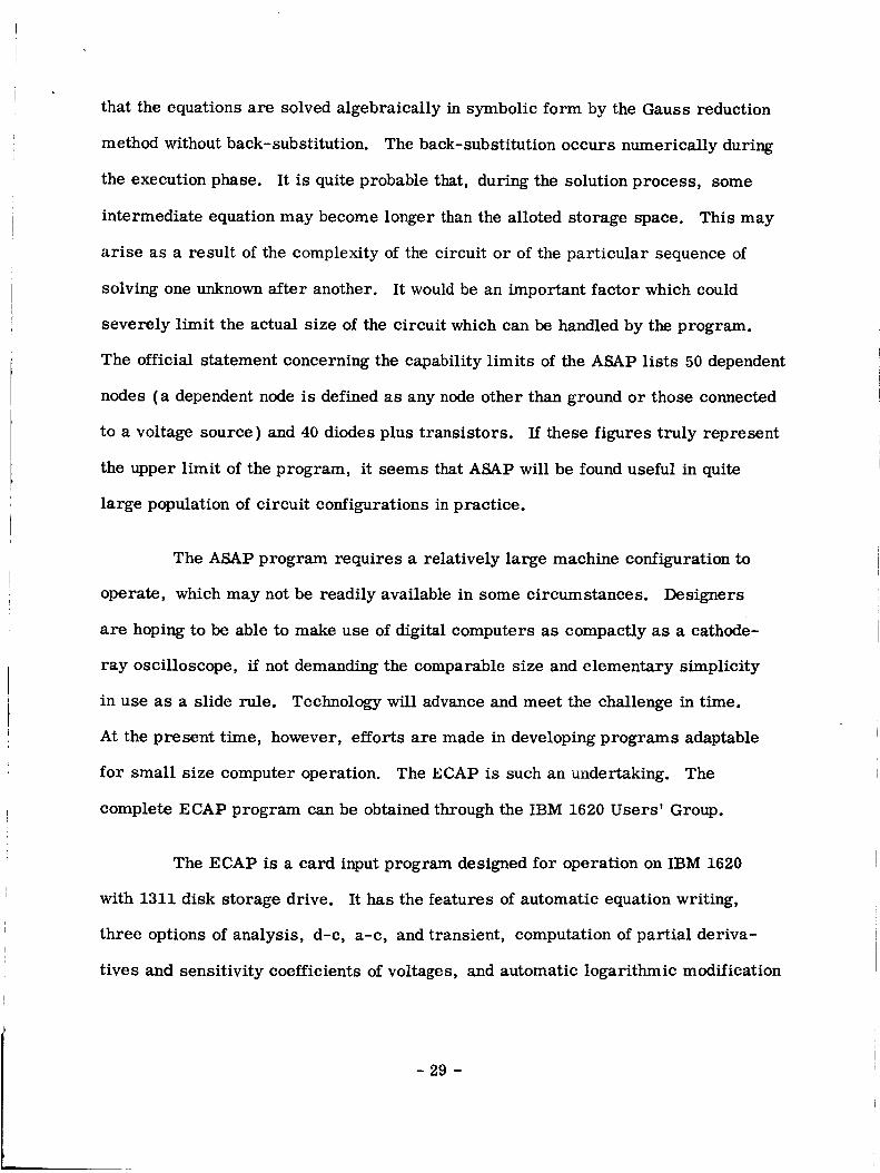
that the equations are solved algebraically in symbolic form by the Gauss reduction

method without back-substitution. The back-substitution occurs numerically during

the execution phase. It is quite probable that, during the solution process, some

intermediate equation may become longer than the alloted storage space. This may

arise as a result of the complexity of the circuit or of the particular sequenceof

solving one unknownafter another. It would be an important factor which could

severely limit the actual size of the circuit which can be handled by the program.

The official statement concerning the capability limits of the ASAP lists 50 dependent

nodes (a dependent node is defined as any node other than ground or those connected

to a voltage source) and 40 diodes plus transistors. If these figures truly represent

the upper limit of the program, it seems that ASAP will be found useful in quite

large population of circuit configurations in practice.

The ASAP program requires a relatively large machine configuration to

operate, which may not be readily available in some circumstances. Designers

are hoping to be able to make use of digital computers as compactly as a cathode-

ray oscilloscope, if not demanding the comparable size and elementary simplicity

in use as a slide rule. Technology will advance and meet the challenge in time.

At the present time, however, efforts are made in developing programs adaptable

for small size computer operation. The ECAP is such an undertaking. The

complete ECAP program can be obtained through the IBM 1620 Users' Group.

The ECAP is a card input program designed for operation on IBM 1620

with 1311 disk storage drive. It has the features of automatic equation writing,

three options of analysis, d-c, a-c, and transient, computation of partial deriva-

tives and sensitivity coefficients of voltages, and automatic logarithmic modification

- 29 -

of frequency in the a-c analysis portion.

Transistors and diodes are represented by their equivalent circuits in the

analysis. In the transient calculations the parameter values of the diode and tran-

sistor can be made to vary as a function of circuit voltages and currents. To

accomplish this, the complement of the circuit elements which are recognized by

ECAP contains a "switch" element, which presents the pertinent equivalent circuit

for a particular operating region. Thus the three commonly referred to regions

of operation of a transistor, cutoff, active, and saturation, can be handled adequately;

in a similar manner the diodes can be conductingwith different forward resistance

or nonconducting.

In the ECAP program the sensitivity coefficients are defined and calculated

only for node voltages as their change for a 1% change in the branch parameter.

In the worst case analysis both worst-case maximum and worst-case minimum are

computed. In the former calculation, positive partial derivatives are multiplied

by positive tolerances and negative partial derivatives by negative tolerances. In

the latter, positive partial derivatives are multiplied by negative tolerances, etc.

The basic assumption is that the circuit output variables are linearly related to the

parameter values. This approximation is valid when the parameter tolerances are

small. When the tolerance exceeds 10% of the nominal value, the manual recommends

the parameter substitution method. First, the partial derivatives of the node voltages

are calculated. Then the nominal value of each parameter in the circuit is replaced

with its maximum or minimum value, in accordance with the sign of the corresponding

partial derivative, and the result is treated as a new ECAP job.

- 30 -

In the d-c analysis program, the d-c parameter modification solutions for

a given circuit are obtained by correcting the nodal impedance matrix or the equiva-

lent current vector associated with the circuit. This imposes the condition that the

tolerance has to be limited in range in the automatic determination of worst cases.

However, the a-c modification solutions, on the other hand, are completely new.

Consequently it allows any extent of parameter change in the calculation.

A maximum of five coupled inductances can be included in the circuit that

is to be analyzed. This is a feature not often found in other programs.

The transient response of node voltages and element currents are produced

by ECAP at the start of a transient solution and at uniform intervals of time there-

after, until the end of the solution is reached. In addition, these output variables

are also produced immediately before and immediately after each switch actuation,

if any. The time of the switch actuation is also given.

The system of integro-differential equations which arises in the transient

analysis is solved in ECAP by an implicit numerical integration technique. It

involves two main tasks: the replacement of the system of integro-differential

equations by an equivalent set of algebraic difference equations, and the repetitive

numerical solution of the algebraic equations. In solving the equations at the end of

each series of discrete intervals of time, each new solution is dependent upon the

results of the previous solution. That is, the values of certain of the terms in the

set of algebraic equations are always computed from the results of the previous

solution. For the first solution (at the end of the first time step} these terms are

evaluated from the circuit initial conditions. Therefore, the results of each solution

become the initial conditions of the succeeding solutions.

- 31 -

References

[1]

[21

[31

International Business Machine Corp., "ASAP, An AutomatedStatistical Analysis Program, " Tech. Rept. prepared

for NASA Goddard Space Flight Center, Greenbelt, Md.,Contract No. NAS 5-3373.

J. N. Hatfield, "A Linear Circuit Analysis Program for the IBM1620/1311 20k Data Processing System: CIRCS, "

Jet Propulsion Lab., Pasadena, Calif., May, 1964.

International Business Machines Corp., "1620 Electronic CircuitAnalysis Program: ECAP 1620-EE-02X," IBM Tech.Publ. Dept., White Plains, N.Y., 1965.

- 32 -

SectionHI Adaption of Current Techniquesof Computer-Aided

Circuit Analysis to Moderate Size Computer

Oneof the areas of interest to the project for investigation is the

possible use of the moderate size computer for circuit analysis. Since the

IBM 1620 digital computer is a relatively small machine and is available on

campus, it was decided to study programming methods that could be performed

using this computer. One method that seemed particularly suitable for pro-

gramming by the IBM 1620 is the scheme used on the British general purpose

computer called Deuce [ 1 ]. This method will give the solution of driving

point and transfer functions of cascaded networks as a function of sinusoidal

frequencies.

The Deuce method of programming was selected for the following

reasons: (1) many practical circuits consist of cascaded stages with simple

network geometry, although the circuits are composed of many components;

(2) it permits and encourages the circuit designer to analyze his design with

a minimum of programming experience in a span of time commensurate with

bread-boarding a circuit; (3) the program can easily be modified to cope with

configurations of various complexities and (4) the program can be run by the

designer on a small computer.

- 33 -

i. The Analysis Procedure

The Deucetype program consists essentially of determining the

steady state behavior of linear networks consisting of a number of three or

four-terminal networks connectedin cascade. The technique is designed

primarily for identical sections in series. The sections may be one of the

following structures: shuntand series branch (ladder network), bridged-T,

or lattice. If the structure varies from one section to another, the most

complicated segment is taken as the parent structure of the configuration.

Other sections are then regarded as special cases of the parent structure by

assigning proper values (either short circuit or opencircuit) at proper places.

In the simple case of an ordinary ladder network, each section is an

L with two branches (Fig. la), one shuntand one series. A program written

to handle the ladder network is included in this report and will be discussed in

detail later. Other programs may bewritten to handle cascadednetworks having

bridged-T or lattice sections as the parent structure (Fig. lb, c, d ).

As an illustration of determining the basic structure of a given network,

consider the network of Fig. 2. Since one section of the network is the bridged-T,

the network is considered a cascade connection of three bridged-T sections,

two of which have branches missing. Once the basic structure is decided, the

equation for driving point and transfer functions are derived. A table of these

functions for all common network configurations can be made and used as

needed in the programs.

- 34 -

The program analysis proceeds step by step beginning with the out-

put terminals of the networks and working toward the input terminals as shown

in Fig. 3. (It could also be developed by proceeding from the input terminals

to the output terminals ).

Each section is analyzed knowing the output voltage and output admittance.

As a starting point, the output voltage V o is assigned the reference value of 1.0

volt at an angle of 0 °, and the output admittance Yo is assigned the value of

zero mhos at an angle of 0°. The input voltage V 1 and input admittance Y1 of

the section are calculated using appropriate equations which have been prepared

by the designer and stored in the program. Thus, in general, with V i and Yi

known, V i + 1 and Yi + 1 of the next section are calculated. This procedure

is continued until the input voltage V n and the input admittance Yn are determined.

Note that although V o is assumed equal to one volt, the actual value of

Vn will ultimately determine the true value of Vo. Similarly, Yo may be other

than zero but this is simply specified at the start of the program, before

Y1, Y2, ..., Yn are computed.

2. Transforming a Network Diagram to Computer Input

In transforming a given circuit diagram to computer input, the basic

component is taken as the series combination of one resistor, one inductor,

and on__eecapacitor. Let this RLC series combination be called a "twig". In

Fig. 4a is shown several possible forms of a twig. Note that two elements of

- 35 -

the same kind, e.g. two resistors, in series, form two twigs. The parallel

connection of two or more twigs is a "nest". A "branch" may be formed by

a twig_ a nest, or a combination of the two. See Fig. 4b and 4c. In the

particular case of a ladder network, the twigs, nests, and branches may

appear either in the series arm or in the shunt arm. As shown in Fig. 5, the

series arm is specified in terms of its impedance and the shunt arm in terms

of its admittance.

The key idea of writing the circuit into the computer input is to assign

a proper code to each and every twig. The code is interpreted by the machine

and thus determines the location of the twig with respect to others in the

basic configuration of the network. A twig may be found in several locations

in the ladder network. For example it may (a) stand alone in series or shunt

arm, (b) be in parallel with other twigs forming a nest, or, (c) be part of a

branch composed of a twig and a nest. This is illustrated in Fig. 6.

It often happens that the network structure requires "dummy" twigs

be introduced. The program is written in such a way that each series branch

and shunt branch must end in a single twig. This twig serves the program control

that causes the total impedance or admittance to be calculated. When the given

structure does not contain the twig, the dummy twig is inserted. The dummy

twig has zero values of inductance, susceptance and resistance and does not

affect calculations other than its use as a program control. The use of the

dummy twig will be included in the ladder example to be worked out in the

following paragraph.

- 36 -

Input data for the circuit to be analyzed are punched on standard 80

column IBM cards. Each twig of the circuit is represented on one IBM card.

In general, each IBM card is divided into a number of fields as illustrated

in Fig. 7. Two fields F (I) and G(I) are used to designate the position of the

twigs in the structure of the cascaded section. Three other fields are used to

indicate the value of the L, C and R components. Note that the type of compon-

ent is designated by giving its value in a specific position of the fields. In the

program, the symbol S (where S = 1/C) is used instead of C, since values of

infinite C cannot be processed by the computer. The symbol H instead of L

was used since L represents a number without a decimal in Fortran program-

ming. If H, S or R are short circuits, the value of zero is entered into the

respective fields.

3. Analysis of a Ladder Network

Consider the ladder network shown in Fig. 5 where it is desired to find

V n and Yn, the input voltage and input admittance respectively, from some

assumed V o and Yo at the output end.

First the equation for the solution of the voltage transfer function

V r + 1/V r and the driving-point admittance Yr per section of the ladder network

are derived by the circuit designer.

Vr+l - l+z 2 (Yr+Yl)Vr

Yr + 1 = mVr (Yr + Yl )Vr+l

- 37 -

where z and y denotebranch impedance (series) and admittance (shunt) respectively,

of each ladder section, and Yr is the input admittance to the section.

Next, it is necessary to decide on a coding scheme in the first two fields,

F (I) and G (I), on the data cards for entering the detailed structure of series and

shunt branches. In the following example of coding, nine different combinations are

possible in stating the location of one twig with respect to others.

F(1) G(1)

1 0

1 1

1 2

-i -I

-i -I

-i -2

0 0

0 -I

0 1

Indicates a twig that is part of a nest.

Indicates a current source G, of value H (I) and angle S (I).

Indicates a voltage source E, of value H (I) and angle S(I).

Indicates a twig that is in series with a nest, both of whichare in the impedance part of the structure.

Indicates a twig that is in series with a nest, both of whichare in the admittance part of the structure.

Indicates only one twig exists in an admittance part of thestructure.

Indicates only one twig exists in an impedancc part of thestructure.

not presently used.

not presently used.

Let us take the specific ladder network of Fig. 8 into consideration. Note

that two branches are made up of single nests. At locations designated by (A) and

(B) dummy twigs must be inserted. Note that these dummy twigs are located at the

high potential ends of the Z and Y branches. The dummy twigs will be the last

elements of the branches examined and will, therefore, terminate the branches.

- 38 -

In order to use the ladder network program, there are three types of input

cards that must be inserted with the program deck. These cards are:

(1) The input control card. This card sets the limits of the four program loops.

Only three of the loops are actually satisfied when solving a problem. In

particular, the control card specifies J, L, M and N where

a) J = the number of twigs in the circuit. The network of Fig. 8 shows

twelve twigs identified by circled numbers. The twigs numbered 4 and

7 are dummy twigs. This loop must be satisfied since J is equal to the

number of input data cards. In the example of Fig. 8, the value of

j is 12.

b ) L = the number of frequencies at which analysis is desired. The

attached program is written to read in five values of frequency-in

radians/sec but could easily be extended. The program calls for 5

values of frequency on the read Statement and, hence, at least 5 values

must be available on the frequency input card. The value of L determines

how many of the 5 frequencies will be used in making analysis computa-

tions. Therefore, L must be 1, 2, 3, 4, or 5. This loop must be satisfied.

c ) M = the number of sections in the complete network. This number tells

the machine when the input terminals have been reached. In the example

of Fig. 8, there are 3 sections. This loop must be satisfied.

d } N = the number of twigs per section. This number varies from one

section to the next. The value of N may be greater than or equal to the

maximum number of twigs per section. This loop need not be satisfied.

In the example of Fig. 8, there are 6 twigs in one section, hence, the

value of N is set to 6 or more.

- 39 -

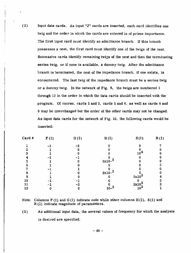
(2) Input data cards. As input "J" cards are inserted, each card identifies one

twig and the order in which the cards are entered is of prime importance.

The first input card must identify an admittance branch. If this branch

possesses a nest, the first card must identify one of the twigs of the nest.

Successive cards identify remaining twigs of the nest and then the terminating

series twig, or if none is available, a dummy twig. After the admittance

branch is terminated, the nest of the impedance branch, if one exists, is

encountered. The last twig of the impedance branch must be a series twig

or a dummy twig. In the network of Fig. 8,. the twigs are numbered 1

through 12 in the order in which the data cards should be inserted with the

program. Of course, cards 2 and 3, cards 5 and 6, as well as cards 8 and

9 may be interchanged but the order of the other cards may not be changed.

As input data cards for the network of Fig. 10, the following cards would be

inserted:

Card # F(I) G(I) H(I) S(I) R(I)

1 -1 -2 0 0 72 1 0 0 0 63 1 0 0 104 0

4 -1 -1 0 0 05 1 0 3x10-3 0 0

6 1 0 0 0 5

7 -1 1 0 0 08 1 0 2x10 -3 0 09 1 0 0 5x103 4

i0 -i -i 0 0 3ii -i -2 0 2x103 212 0 0 10 -3 103 1

Note:

(3)

Columns F (I) and G(I) indicate code while other columns H(1), S(I) and

R (I) indicate magnitude of paramehters.

As additional input data, the several values of frequency for which the analysis

is desired are specified.

- 40 -

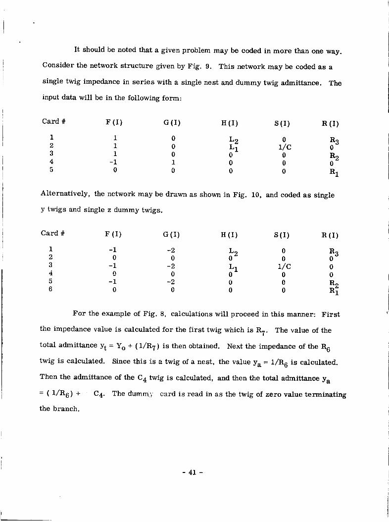
It shouldbe notedthat a given problem may be codedin more than one way.

Consider the network structure given by Fig. 9. This network may be codedas a

single twig impedancein series with a single nest and dummy twig admittance. The

input data will be in the following form:

Card # F (I} G(I} H(I) S(I) R (I}

1 1 0 L2 0 R32 i 0 L I I/C 03 1 0 0 0 R 24 -1 1 0 0 0

5 0 0 0 0 R 1

Alternatively, the network may be drawn as shown in Fig. 10, and coded as single

y twigs and single z dummy twigs.

Card # F (I) O(I) H(1) S(I) R(I)

1 -1 -2 L 0 R 32 0 0 0 2 0 0

3 -i -2 L 1 I/C 04 0 0 0 0 05 -I -2 0 0 R,,

6 0 0 0 0 R_

For the example of Fig. 8, calculations will proceed in this manner: First

the impedance value is calculated for the first twig which is R 7. The value of the

total admittance Yt = Yo + ( l/R7 ) is then obtained. Next the impedance of the R 6

twig is calculated. Since this is a twig of a nest, the value Ya = 1/R6 is calculated.

Then the admittance of the C 4 twig is calculated, and then the total admittance Ya

= (l/R6) + : C 4. The dummy card is read in as the twig of zero value terminating

the branch.

- 41 -

In a similar fashion the total impedance is obtained for the series branch.

As a consequence, we have

V 1 = V o [ 1 + (total admittance ) (total impedance)]

Y1 = (total admittance)_ (Vo/V 1 )

The program then moves on to the section 2.

In section 2, the twig containing L 3 is encountered. The impedance is

calculated as L 3 and the admittance becomes 1/ L 3. Next the twig R 5 is read.

The impedance is calculated and the admittance becomes (1/R 5 ) + (1/ L 3 ).

Finally the dummy card is read and the total admittance Yt = (1/RS) + ( 1/ L 3 )

+ Y1 is obtained.

The process is repeated until the input terminals are reached.

The complete write-up of the computer program for analyzing the ladder

structure of Fig. 5 is contained in AppendLx B of this report. It follows the flow

chart Fig. 11 and involves four iterative loops of operation. They can be explained

as follows.

Block 1

The parameters read here refer to: the number of twigs in the network;

the number of frequencies at which analysis is desired; the number of sections in

the total network; the maximum number of twigs in a section.

Block 2

The code and value of each twig is read and stored in the memory.

- 42 -

Block 3

The number of values of frequency at which analysis is desired are read

and stored in the memory.

Blocks 4, 5 and 6

Initial values of output voltage and output admittance are specified. Note

that some of these conditions are within loops and, hence, are executed more or less

times than others.

Block 7

The impedance of a twig is calculated by separating the real and imaginary

parts and then obtaining the magnitude of the impedance and the associated phase

angle.

Block 8

The code of the twig being operated upon is identified.

is chosen.

One of six subroutines

Blocks 9, 10, 11, 12, 13, 14

Each twig is identified as having a form which must be handled by one of

these subroutines. Only one of these subroutines is used for any one twig.

Block 15

At this point, a decision is made. If the loop has been repeated N times,

then there are no more twigs in the section and the program precedes to Block 16.

If not, the program begins operating on the next twig.

- 43 -

Block 16

The input voltage to the section just operated upon is calculated along with

the appropriate phase angle.

Block 17

The input admittance to the section just operated upon is calculated along

with the appropriate phase angle. This completes the calculations for this section.

Block 18

The calculated values of input voltage and input admittance of the section

are assigned as the output voltages and output admittance for calculations of the

next section.

Block 19

At this point, a decision is made. If the section just handled was the final

section, then the values of input voltage and associated angle as well as input

admittance and angle are punched as output data. If the _ection was not the final

section, loop M is followed which then causes calculations of the next section to

begin.

Block 20

It is at this point that output data is punched. The program is written to

punch output data at the end of each section and at the end of the last stage. If only

the input voltage and admittance are needed, the extra punch statement may be

deleted. (Extra punch statement not shown in flow diagram. The statement would

occur between Blocks 18 and 19.)

- 44 -

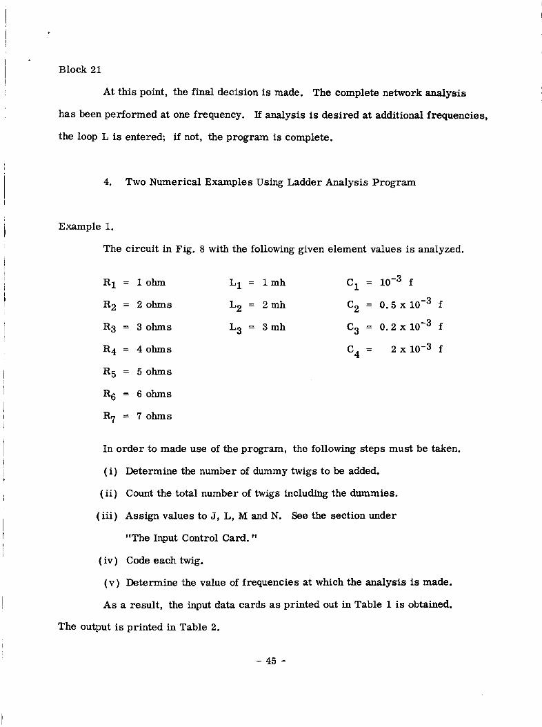
Block 21

At this point, the final decision is made. The complete network analysis

has been performed at one frequency. If analysis is desired at additional frequencies,

the loop L is entered; if not, the program is complete.

4. Two Numerical Examples Using Ladder Analysis Program

Example 1.

The circuit in Fig. 8 with the following given element values is analyzed.

R 1 = lohm

R 2 = 2 ohms

R 3 = 3 ohms

R 4 = 4 ohms

R 5 = 5 ohms

R 6 = 6 ohms

R 7 = 7 ohms

L 1 = lmh C 1 = 10 -3 f

L 2 = 2mh C 2 = 0.5x10 -3 f

L 3 = 3mh C 3 = 0.2x10 -3 f

C 4 = 2 x 10 -3 f

(i)

(ii)

( iii )

In order to made use of the program, the following steps must be taken.

Determine the number of dummy twigs to be added.

Count the total number of twigs including the dummies.

Assign values to J, L, M and N. See the section under

"The Input Control Card."

(iv) Code each twig.

(v) Determine the value of frequencies at which the analysis is made.

As a result, the input data cards as printed out in Table 1 is obtained.

The output is printed in Table 2.

- 45 -

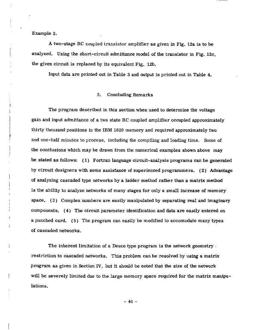
Example 2.

A two-stage RC coupledtransistor amplifier as given in Fig. 12a is to be

analyzed. Using the short-circuit admittance model of the transistor in Fig. 12e,

the given circuit is replaced by its equivalent Fig. 12b.

Input data are printed out in Table 3 andoutput is printed out in Table 4.

5. Concluding Remarks

The program described in this section when used to determine the voltage

gain and input admittance of a two state RC coupled amplifier occupied approximately

thirty thousand positions in the IBM 1620 memory and required approximately two

and one-half minutes to process, including the compiling and loading time. Some of

the conclusions which may be drawn from the numerical examples shown above may

be stated as follows: { 1) Fortran language circuit-analysis programs can be generated

by circuit designers with some assistance of experienced programmers. (2) Advantage

of analyzing cascaded type networks by a ladder method rather than a matrix method

is the ability to analyze networks of many stages for only a small increase of memory

space. (3) Complex numbers are easily manipulated by separating real and imaginary

components. (4) The circuit parameter identification and data are easily entered on

a punched card. (5) The program can easily be modified to accomodate many types

of cascaded networks.

The inherent limitation of a Deuce type program is the network geometry :

restriction to cascaded networks. This problem can be resolved by using a matrix

program as given in Section IV, but it should be noted that the size of the network

will be severely limited due to the large memory space required for the matrix manipu-

lations.

- 46 -

References

[i] E. A. Pacello, "The Use of Deuce for Network Analysis." Marconi Review,vol. 24, pp. 101-114; 1961.

- 47 -

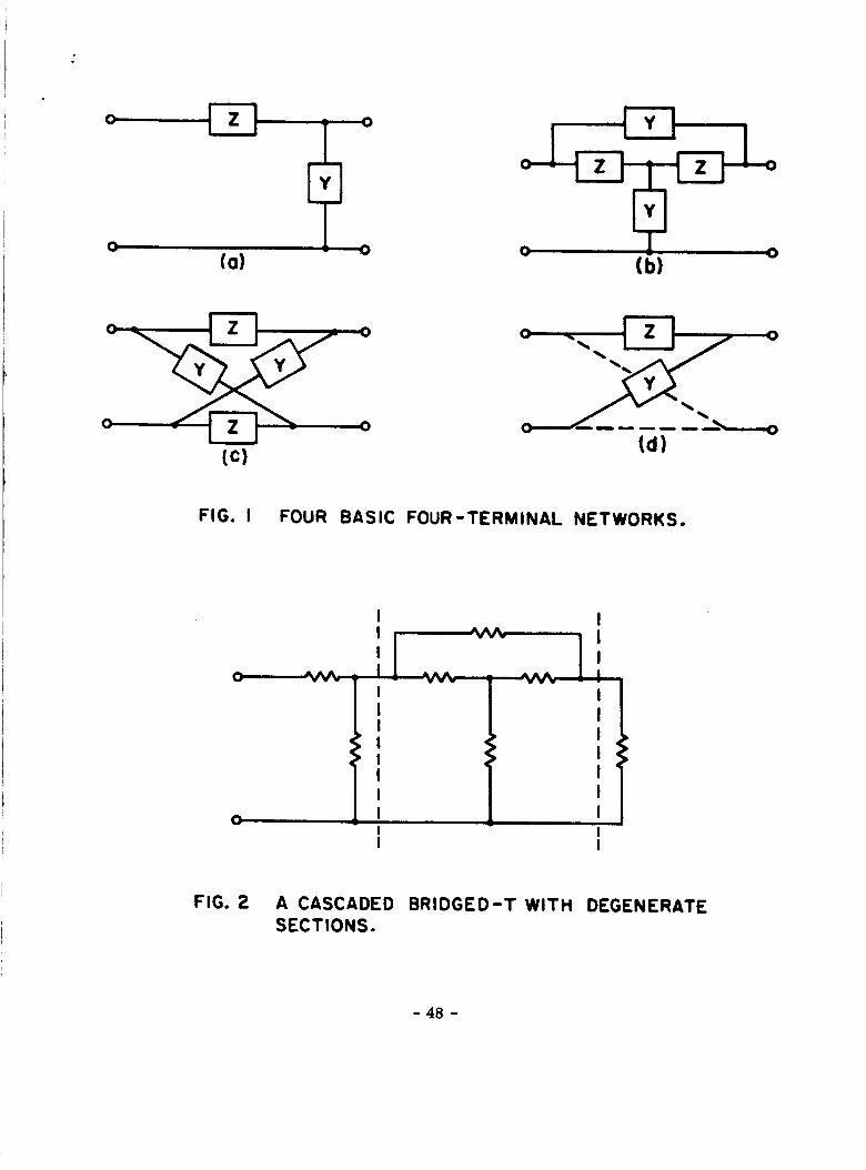
O i

Eo

(o) (b)

(c)o---.,,'_--- --",----,o

td)

FIG. I FOUR BASIC FOUR-TERMINAL NETWORKS.

II

1c _ I _

III

:iIIIII

I

o

I

I'I_ I

IIII

'IIIII

FIG. 2 A CASCADED BRIDGED-T WITH DEGENERATESECTIONS.

- 4:8 -

Yn

o----.--

Vn-I vz vl Vo

Yn- I-"" Y2 -'_ YI

-.------0

0

FIG. 3 CASCADED NETWORK CONFIGURATION.

(a) (b)

];

(c)

FIG. 4 SEVERAL VARIATIONS OF A TWIG (0),

A NEST (b), AND A BRANCH (C).

- 49 -

0

Vn-i II Vl

I II I

yn__ I yl---_ !I

I. I

I II

I I

II

EEFl- Ovo

FIG. 5 A LADDER NETWORK.

o c

b

0

0

C

b bi_b

' 0

FIG. 6 (o) TWIGS STANDING ALONE; (b) TWIGS IN

A NEST; (c) TWIGS IN BRANCHES COMPOSED

OF OTHER NESTS.

- 50 -

COLUMN

r(x)G(i)iIi

!

I

9-23 24-38 39-53 54-80

H(I! S(l! FIIII UNUSED

FIG. 7 FIELDS OF AN IBM CARD

v i

0

® ®

®I._ _.,C-_., o_.., vo

FIG. 8 AN RLC LADDER

- 51 -

C

0

DUMMY

/R 2

LI IL2

: i C R3

(CARD d! 4)

o

o

FIG. 9 AN INVERTED L SECTION.

C

0

DUMMY (CARD -11k4}

DUMMY (CARD :ilk2)., /'

] °iI

R 2 ,

0

FIG. I0 AN ALTERNATE FORM OF

INVERTED L SECTION.

- 52 -

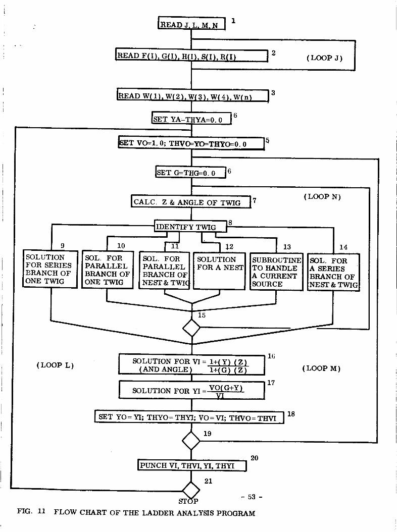
IREAD J.L. M. N 1

]READ F(I), G(I) I Ht

, ,, ,,,

[READ W( 1 ), W( 2 ),

), S(I), R(I) ] 2

i,,,

_ r{3), W(4), W{n } ]3

ii

_ET VO=I. 0; THVO=YO=THYO=0.0 15

. i i_ i i HH ill

l[SET G=THG=O.O ]6

]CALC. Z & ANGLE OF TWIG [7

'IIDENTIFY TWIG

(LOOP J)

i

(LOOP N)

9

SOLUTION

FOR SERIES

BRANCH OF

ONE TWIG

10 11 12 13

SOL. FOR SOL. FOR SOLUTION SUBROUTINE

PARALLEL PARALLEL FOR A TO HANDLEBRANCH OF BRANCH OF A CURRENTONE TWIG SOURCE

14

SOL. FOR

A SERIES

BRANCH OF

NEST &

15

(LOOP L) I16

SOLUTION FOR VI : 1+(Y) (Z)

(AND ANGLE _ I+(GI {Z)

[ SOLUTION FORIyI = VO(G+Y) i 17VI

|

I[ SET YO: YI; THYO: THYI; VO= VI; THVO= TI-IVI

i

19 20

IPUNCH VI, THVl, YII THYI

- 53 -

18

(LOOP M)

FIG. 11 FLOW CHART OF THE LADDER ANALYSIS PROGRAM

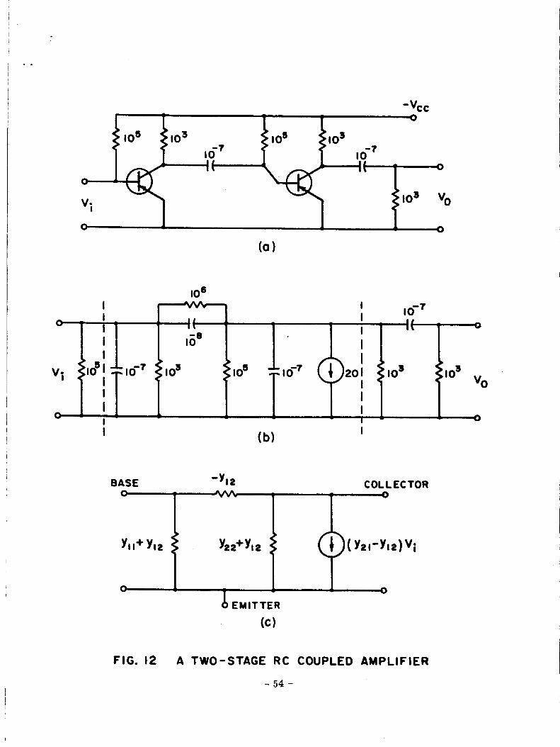
-Vcc

(o)

i0 s

Ii _ il I°-7

°l i ' • '! 'Vi ! iTiO51 IO-7 llo3 llo5 IO-7 20 IOs

C I , * 0

I (b) I

BASEC

Y,i+ Y,,

C

-Ylz COLLECTORo

Yz_+Yl_ (Yzl-Yl2)V I

i 0

_) EMITTER

(c)

FIG. 12 A TWO-STAGE RC COUPLED AMPLIFIER

- 54 -

12" 3

-1t -_o

10 Oo

10 O,

-lo -1,

lo O,

lo O,

-lo Le

lo Oo

lo O,

-!o -le

-lo -20

O, 60

500E02

I

0,0600

O,OEO0

O,OEO0

O,OEO0

300E-3

O,OiO0

O,OEO0

2,0d-3

O,OEO0

O,OEO0

O,OEO0

1,OE-3

I.OE03 2,0E03

O,OEOO

O-OEO0

I-OE04

O,OEO0

O,OEOO

O.OEO0

O,OEOO

O-OEO0

5-0E03

O,OEO0

2,0E03

1-OE03

O,OEO0

7,0EO0

600EO0

O,OEO0

O,OEO0

O,OEOO

500EO0

O,OEO0

O,OEO0

4-OEO0

3-OEO0

2,0EO0

I,OEO0

O*OEO0

- 55 -

TABLE 2

C° -C

Ib,6OE-O2 .00E-99

17.40E-02 29.14E-02

18.01E-OI-13*I3E-02 79,28E-03 13,13E-02 50 • OOE+O I

66,66E-02 15,70E-01

69.60E-02 12,79E-01

IO.OOE-OI 15.70E-01

I0.86E-01 15,39E-01

54.96E-01 49.76_-02 24.00E-02 55,14E-02 50.OOE+Ol

98.81E-01 42.48E-02 24.79E-02 89,20E-02 50,00E+01

9.88168f19E+O0 4,2481755E-01

16.66E-02 .00E-99

19,43E-02 54,04E-02

Ib,73E-OI-22,79E-02 85,36E-03

2.4799813E-01 8.9207560E-01

22,79E-02 lO.OOE+02

33,33E-02 15.70E-01

38.87E-02 I0-30E-01

50,00E-02 15.70E-01

62.95E-02 14.15E-01

43.00E-01 4B,OBE-03

61.80E-01 29.55E-02

17,59E-02

36.73E-02

61,82E-02 IO,OOE+02

48.24E-02" lO.OOE+02

6.1dO7711E+O0 2,9552675E-01

16.66E-02 .00E-99

26,03E-02 87,60E-02

14,15E-OI-30,23E-02 I0,09E-02

3,6731263E-01 4,8245680E-01

30,23E-02 20,00E+02

16.66E-02 15,70E-01

26,03E-02 69.47E-02

25.00E-02 15,70E-01

40.45E-02 i I,IOE-OI

37.57E-OI-24,58E-02 13,39E-02 52,94E-02 20.00E+02

57.29E-01 50-57E-02 38*10E-O2-27,27E-02 aO,OOE+02

5,0000000E+02

I,O000000E+03

- 56 -

TABLE 3

27 5

-1 • -2.

Oo O.

lo Oo

lo lo

lo O.

1. C_o

I. O.I. Oo

-I. -I.

Io O.

I. Oo

I. Oo

-I. IoOo Oo

Io Oo

I. Io

I. O.

I. O.

-I. I.

10 O,

I. Oo

-I. -I.

Io O.I. O.

-IoO 1.0O. O.

I •OEO0

8

O.OEO0

O.OEO0

O.OEO0

2.0E01

O.OEO0

O.OEO0

O.OEO0

O.OEO0

O.OEO0

O.OEO0

O.OEO0

O.OEO0

OoOEO0

OoOEO0

OoOEO0

OoOEO0

2.0EO1

O.OEO0

OoOEO0

O.OEO0

O.OEO0

O.OEO0

O.OEO0

O.OEO0

O.OEO0

OoOEO0

OoOEO0

1,0E03 I.OE04

OoOEO0

I.OE07

OoOEO0

OoOEO0

O.OEO0

I.OE07

OoOEO0

OoOEO0

I,OE08

O.OEO0

O.OEO0

I.OE07

O.OEO0

O.OEO0

I.OE07

O-OEO0

O.OEO0

O.OEO0

IoOE07

O.OEO0

OoOEO0

1.0E08O.OEO0

IoOE07

OoOEO0

O.OEO0

O.OEO0

I.OE05

1.0E03

O.OEO0

loOE03

O.OEO0

I.OE05

O.OEO0

O.OEO0

1.OE06

OoOEO0

OoOEOO

1.0E03

O.OEO0

I-OE03

O.OEO0

OoOEO0

I.OE03

O.OEO0

I.OE05

O.OEO0

O.EO0

I.OE06

OoOEO0

OoOEO0

OoOEO0

I,OE03

OoOEO0

OoOEO0

IoOE06

- 57 -

TABLE

IO,OOE+O3-15,70E-01 IO,OOE-O8 15,70E-01 IO*OOE-OI

IO.OOE-04 eOOE-99

IO.IOE-04 eOOE-99

IO.IOE-04 99eOOE-06

I0.00E-07 eOOE-99

IO.OOE-07 99o99E-04

50.55E-O2,47oI2E-OI 19.78E-03 98o54E-04 lOoOOE-Ol

lOoOOE-04 o00E-99

IO.OOE-04 99*99E-06

20.00E-04 49e99E-06

II°OIE+O4-62.73E-OI IO.OOE-08 15o70E-01 lOoOOE-01

IO.OOE-04 .00E-99

IO.IOE-04 o00E-99

IO.IOE-04 99.00E-06

IO.OOE-07 o00E-99

IO.OOE-07 99.99E-04

55.6oE-OI-9_elSE-01 19.78E-03 98.54E-04 IO.OOE-OI

10.00E-08 15.70E-01

IO.OOE-04 99.99E-06

55.66E-OI-94.15E-01 20.78E-03 93.84E-04. lO.OOE-Ol

5.5666943E+00 -ge4153038E+O0 2eO784913E-02 9e3848923E-03

lO.04E+OO-14oTIE-O1 99.50E-06 14.71E-01 IO.OOE+02

leOOOOOOOE+O0

I0.00E-04 .00E-99

IO.IOE-04 .00E-99

I0.14E-04 98.6BE-03

IO.OOE-07 .00E-99

I0.04E-06 14.71E-01

52.3bE-OS-44.10E-OI 19.28E-02 12.69E-01 IO.OOE+02

IO.OOE-04 .00E-99

I0.04E-04 99o66E-03

20.02E-04 49.95E-03

IO.14E-OI-47.21E-OI 99.95E-06 15o70E-01 IO.OOE+02

I0.00E-04 .00E-99

IO.IOE-04 .00E-99

10.14E-04 98.68E-03

I0-00E-07 .00E-99

I0.04E-06 14.71E-01

52*3bE-O6-Tb. SOE-OI 19.40E-02 12.6bE-01 IO.OOE÷02

IO.OOE-05 15eTOE-01

I0.04E-04 99o66E-03

52.36E-O6-76.58E-01 19.50E-02 12.61E-01 IO.OOE+02

5o2363348E-05 -7.65876Z6E+O0 1.9506404E-01 1.2616574E+00

14*14E-OI-TBe53E-02 70.71E-05 7B.53E-02 IO.OOE+03

I.O000000E+03

lOeOOE-04 eOOE-99 -58-

"IO,IOE-04 ,00E-99

14o21E-04 78eO4E-02

lOeOOE-O7 eOOE-99

lO,OOE-05 15,60E-01

15,SbE-OS-31o12E-Ol 90,89E-02 74,6dE-02 IO,OOE+03

IOoOOE-04 o00E-99

14o14E-04 78o53E-02

22e3bE-04 46,36E-02

14,18E-O2-39,36E-OI 99,92E-05 15,69E-01 IO,OOE+03

IOoOOE-04 o00E-99

10, IOE-04 eOOE-99

14,21E-04 78eO4E-02

IO,OOE-07 eOOE-99

10oOOE-05 15,60E-01

16,53E-O6-59o56E-01 85,83E-02 43,92E-02 10oOOE+03

IO,OOE-04 15,70E-01

l_o14E-O_ 7B,53E-02

Ib,53E-O6-59,SbE-01 85o96E-02 43o97F--02 lO.OOE+03

Io6531502E-05 -5,9567135E+00 8o_965164E-01 4e3979027E-Ol

lOo04E-OI-99,66E-03 99o50E-05 99,6bE-03 IO,OOE+04

IOoOOE-04 ,00E-99

IOolOE-04 o00E-99

I0o05E-03 14o70E-01

IOoOOE-07 ,00E-99

I0,00E-04 15ebgE-Ol

56e67E-OS-IBe48E-OI 17,73E-01 17o 78E-02 10 o OOE÷04

I0.00E-04 .00E-99

I0.04E-03 14.71E-01

i0.19E-03 13o73E-01

lO.08E-O2-32o30E-OI 99.B9E-04 15.65E-01 IO,OOE+04

IOoOOE-04 o00E-99

lOelOE-04 ,00E-99

I0.05E-03 14eTOE-O1

I0,00E-07 eOOE-99

IO.OOE-04 15e69E-Ol

foe5 E-O5-4Bo52E-OI 95,16E-02 50o75E-03 IO,OOE+04

IOQOOE-03 15eTOE-Ol

I0,04E-03 14e71E-01

lOo59E-OS-4B,52E-Ol 95o32E-02 61,17E-03 IOoOOE+04

1,0595160E-04 -4,8523403E+00 9o5324231E-01 6,1179165E-02

lOeOOE-Oi-99o99E-04 99,99E-05 99,99E-04 lO,OOE+05

lOIOOE-04

lOolOE-04

10eOOE-02

IO,OOE-07

_00E-99

eOOE-99

15o60E-Ol

eOOE-99- 59 -

I*O000000E÷04

1,0000000E+05

10,OOE-03 15,70E-01

55,0 1 E-04- 15,98E-0 1 IB,17E-OI

lO,OOE-04 ,00E-99

IO,OUE-02 15,60E-O1

lO,OOE-02 15,50E-01

lO,09E-O2-30,37E-OI 99,42E-03

I0.00E-04 ,00E-99

lO,IOE-04 ,00E-99

IO,OOE-O2 15,60E-0|

lO*OOE-07 ,00E-99

IO*OOE-03 15.70E-01

lO,57E-O4-46,37E-O1 95.55E-02

IO,OOE-02 15*70E-01

IO,OOE-02 15,60E-01

IO,57E-O4-46*37E-OI 96.57E-02

I*0571774E-03 -4*b37989bE+O0

23,17E-03 IO,OOE÷05

15.16E-01 IO.OOE÷05

40,48E-03 IO,OOE+05

14.40E-02 IO,OOE+05

9,6578132E-01 1,4408966E-01 I,O000000E+06

- 60 -

Appendix A

The Ladder Network Program was written in such a way

that nine possible codes could be used. To identify twigs,

current sources and voltage sources only seven codes were

used. Nine codes were, therefore, more than enough to

enter appropriate subroutines in the case of the simple

ladder network program. When writing programs to handle

more complex network structures, it is obvious that a

greater number of subroutines will be used and, hence, a

greater number of code combinations will be needed. The

following sequence of IF statements can be used to enter

any one of seventeen subroutines:

IF (F(I)) i, 2, 3

1 IF (G(1)) 4, I0, 5

2 IF (G(I)) ii, 12, 13

3 IF (GCI)) 6, 14, 7

4 IF (F(I) -G(I)) 15, 16, 17

5 IF (F(I) + G(I)) 18, 19, 20

6 IF (F(1) + G(1)) 21, 22, 23

7 IF (F(_) -G(1)) 24, 25, 26

- 61 -

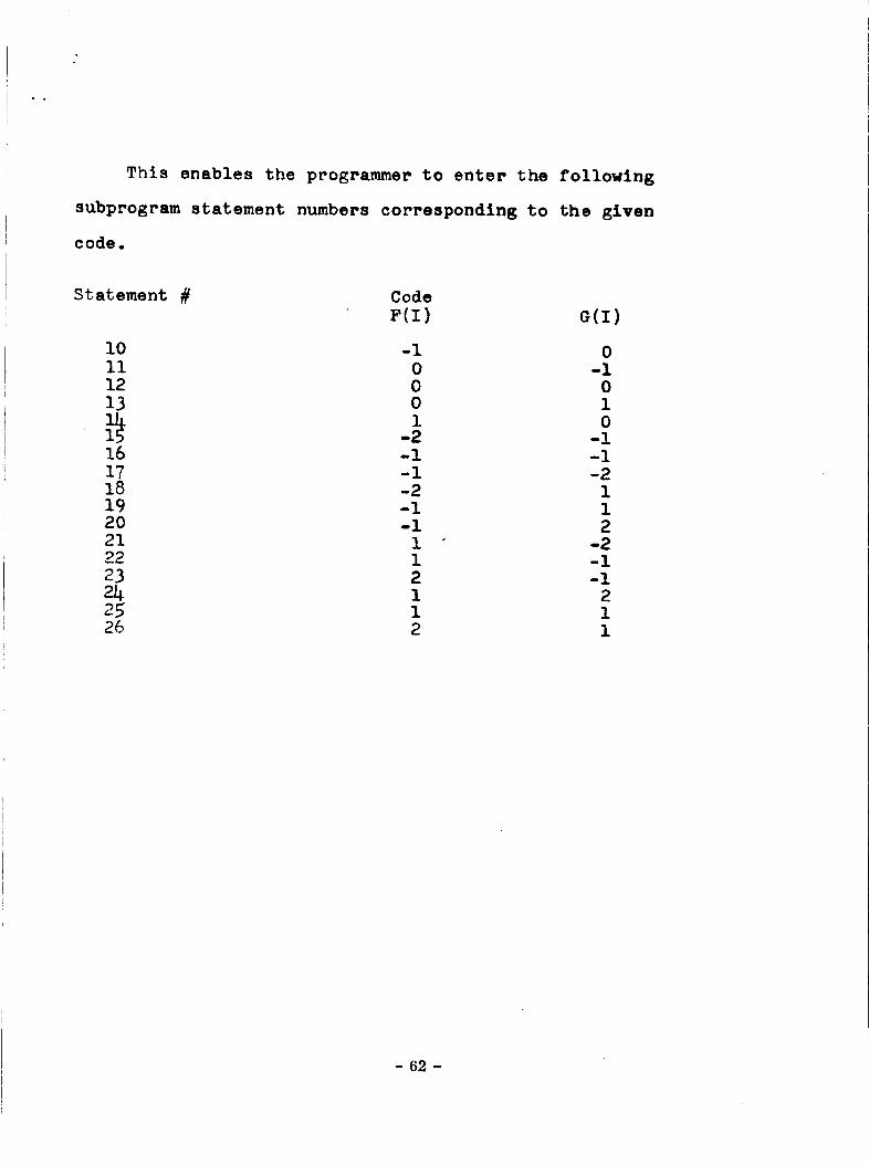
This enables the programmer to enter the following

subprogram statement numbers corresponding to the given

Code.

Statement # Code

F(1) G(1)

I0 -I 0

II 0 -i12 0 0

13 0 li 0

I_ -2 -I

16 -1 -I17 -I -2

18 -2 I19 -I 12O -i 2

21 1 -2

22 1 -i

23 2 -i24 I 225 z l26 2 1

- 62 -

-_ IF(a(1))I

-I,0

+

J

"[IF(F{I))_

. IF(G(I) )I0,-I 0,0

÷

i IF( (I

l1,0

-2,1

P(O(I)+H{I

fI,-2 I,-i 2,-i

-I,i -i,2 i_2 i,i 2,i

- 63 -

APPENDIX B

- 64-

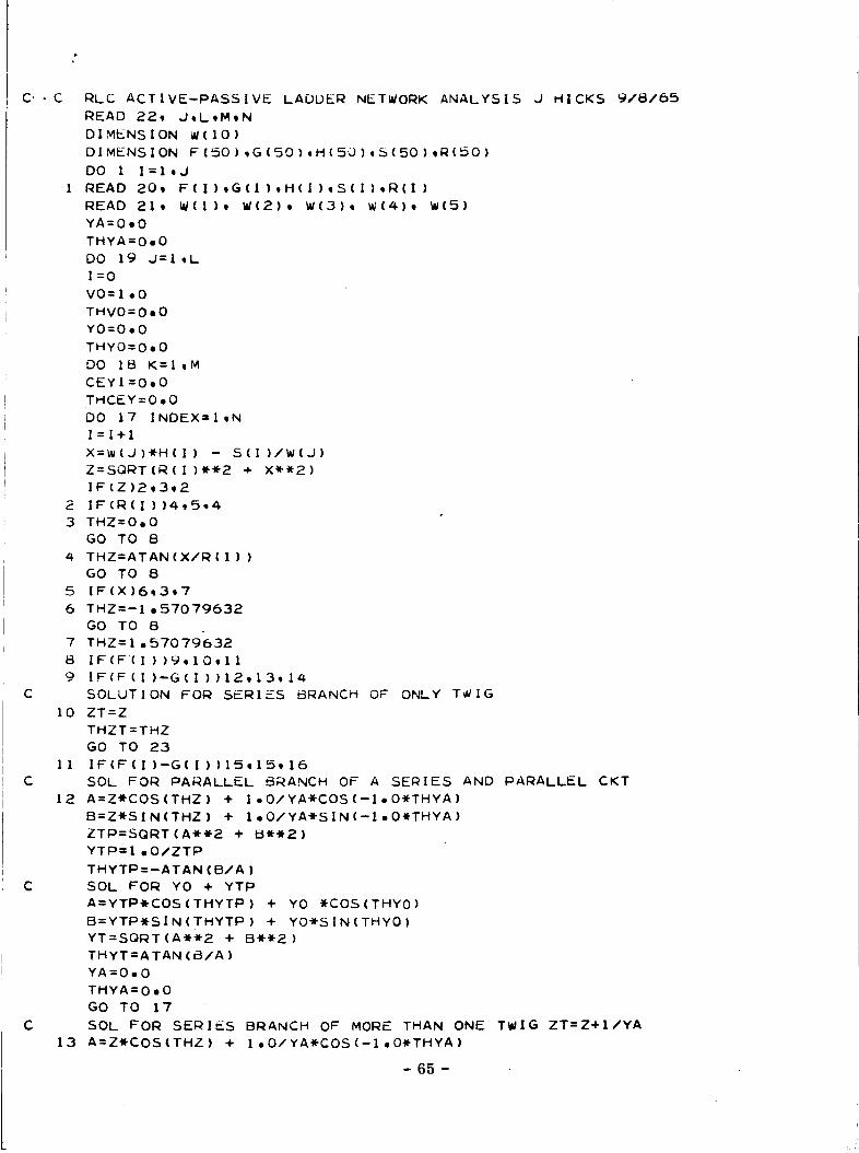
C" • C RLC ACTIVE-PASSIVE LADDER NETWORK ANALYSIS J HICKS 9/8/65

READ 22, J,L,M_N

DIMENSION W(IO)

DIMENSION F(50),G(50),H(5Q)qS(50),R(50)

DO I I:l,J

! READ 20, F(1),G(1),H(I ),S(L),R(1)

READ 21, W(I I, W(2), W(3), W(4), W(5)

YA=OeO

THYA=0.0

DO 19 J=l,L

I=O

VO=l,O

THV0=0.0

YO=0=0

THY0=0=0

DO 18 K=IiM

CEYI=OoO

THCEY=OoO

DO 17 INDEXmI,N

I=l+l

X=W(J)*H(I ) - S(I )/W(J)

Z=SQRT(R(1)**2 + X**2)

IF(Z)2,3,2

2 IF{R(1))4,5,4

3 THZ=OeO

GO TO 8

THZ=ATAN(X/R(I) )

GO TO 8

5 IF(X)6.3,7

6 THZ=--l.57079632

GO TO 8

7 THZ=lo57079632

8 IF(F'(I ) )9,10.11

9 IF(F(I )-G(I ))12,13.14

C SOLUTION FOR SERIES _RANCH OF ONLY TWIG

I0 ZT=Z

THZT=THZ

GO TO 23

II IF(F(I)--G(I))lS,15,16

C SOL FOR PARALLEL 8RANCH OF A SERIES AND PARALLEL CKT

12 A=Z*COS(THZ) + loO/YA*COS(-IoO*THYA)

B=Z_SIN(THZ) + IoO/YA*SIN(--loO*THYA)

ZTP:SQRT(A**2 + B**2)

YTP=I.O/ZTP

THYTP=--ATAN(B/A)

C SOL FOR YO + YTP

A=YTPtCOS(THYTP) + YO tCOS(THYO)

B=YTP_SIN(THYTP) + YO_SIN(THYO)

YT=SQRT(A**2 + B**2)

THYT=ATAN(B/A)

YA=OoO

THYA=OeO

GO TO 17

C SOL FOR SERIES BRANCH OF MORE THAN ONE

13 A=Z*COS(THZ) + loO/YA*COS(-loO*THYA)

TWIG ZT=Z+I/YA

- 65 -

C

C

C

I4

15

16

B=Z*SIN(THZ) + IoO/YA*SIN(-IoO*THYA)

ZT=SQRT(A**2 + B**2)

THZT=ATAN(B/A)

YA=OoO

THYA=OeO

GO TO 23

SOLUTION FOR PARALLEL

A:IoO/Z*COS(-I,O*THZ)

B:IoO/Z*SIN{-IoO*THZ)

YT=SQRT(A**2 + B'w2)

THYT=ATAN(B/A)

GO TO 17

CEYI=H(1)

THCEY:S(1)

GO TO 17

SOLUTION FOR NEST YA=I/Z+YA

A=IoO/Z*COS(-leO*THZ) +

B:IoO/Z*SIN(-IoO*THZ) +

YA:SQRT(A**2 + B_*2)

THYA:ATAN(B/A)

PUNCH 24o YAt THYA

CONTINUE

_RANCH WITH ONLY

+ YO*COS(THYO)

+ YO*SINITHYO)

VA*COS(THYA)

YA*SIN(THYA)

ONE

SOLUTION FOR VI:VO(IoO+YT*ZT)/IIoO-CEYI*ZT)

W(J)

W(J)

- 66 -

TWIG

I?

23 YTZ:YT*ZT

THYTZ=THYT + THZT

C SOLVE FOR C=lo0 + YTZ

A=le0 + YTZ_COS(THYTZ}

B=YTZ_SIN(THYTZ)

C=SQRT(A_2+B_*2)

THC=ATAN(B/A)

CZT=CEYI_ZT

THCZT=THCEY+THZT

A=IeO-CZT_COS(THCZT)

B=-CZT*SIN(THCZT)

E=SQRT(A**2 + B_*2)

IF(A)3Oi31q3!

30 THE=ATAN(B/A) + 3o14159264

GO TO 32

31 THE=ATAN(B/A)

32 VI=VO*C/E

THVI=THVO+THC-THE

C YI=CEYI + YTeVO/Vl

D=YT*VO/Vl

THD=THYT+THVO-THVl

A=CEYI*COS(THCEY)+D*COS(THD)

B=CEYI*SIN(THCEY) + D*SIN(THD}

YI=SQRT(A**2+B**2)

THYI=ATAN(B/A)

PUNCH 24, Vl q THVI, YI, THYI i

YO=YI

THYO=THYI

VO:Vl

18 THV0=THVI

PUNCH 21, Vlt THVI, YI, THYI,

19 CONTINUE,

YP=I/Z+YO

,20 FORMAT(2F4,0_ 3Elb,8)

21 FO-MATI5EI5,?)

22 FORMAT{414)

24 FORMAT (5EI0,2/}

STOP

END

- 67 -

Section IV On-Line Experience in the Time-

Sharing Computing System

In celebration of M.I.T.'s Centennial Year, the School

of Industrial Management of bhe Massachusetts Institute of

Technology sponsored a series of evening lectures on the

theme, "Management and the Computer of the Future" in

March 1961. During one of the sessions Professor John

McCarthy discussed the time-sharlng computer systems Ill

and introduced the notion of a community utility capable of

supplying computer power to each "customer" where, when and

in the amount needed. Such a utility would in some way be

similar to an electrical power distribution system. There

is a large, very large computer complex in some place.

Computing services may be obtained at different locations

by "inserting a plug into the wall". The time-sharlng

computer system interacts with many simultaneous users

through a number of remote consoles. Such a system will

look to each user like a large private computer. This idea

goes quite a while back 12], 131, but only recently has it

caught wide attention and keen interest in the computing

profession. Its experimentation at M.I.T. bears the name

of the research project MAC [41. Other large tlme-sharing

computer systems known in operation include those at System

Development Corporation and Carnegie Institute of Technology.

- 68 -

QUIKTHAN i5_, developed by the International ousiness

Machines Corporation and Desk Side Computer System [6],

developed by the General Electric Company are offered on

a commercial basis.

The present computation facilities for academic

activities at Villanova University consist of the IBM 1620

Data Processing System. On a first-come-first-served basis,

the Comput'ng Center has seen so many instances of over-

crowding of many jobs to be processed in the rush hour, and

of the inconvenience and frustration of the waiting period

before one can get on the computer again in order to fix a

misplaced comma in the program. In taking advantage of the

time-sharing computing serivce of the General Electric

Company, a direct tie line has been established between

Villanova University and the General Electric Computer

Center at Valley Forge, Pennsylvania, since September 1965.

Villanova University is one of the 85 users that time

share the General Electric Computer Complex at Valley Forge.

The main frame is the GE 235 Computer with a 20-bit word

len_th and 6 microsecond core memory. The terminal

teletypewriter at the user's _n,d does not reach the central

processing unit directly; it is first connected to an

intermediate computer called Datanet 30 which is analogous

to a telephone operator between the main switchboard and the

telephone subscribers. Presently there are fifteen lines

- 69 -

associated with the CPU through Datanet 30.

The teletype console accepts keyboard input and/or

paper tape input. The tie line is rented from the local

Bell Telephone Compsny. The user is allowed to store 32

programs in the computer, each of which is limited to

6,000 characters. He can exercise the option of either

using a stored program or submitting a new program in

operation. Associated with the Datanet 30 is a mass

storage system disk of 20 million bits in BCD form. The

computer spends l0 seconds with the user at each round.

The Datanet 30, however, is asynchronous in serving the

users. There are four Datanet 30 system units for the

pool of 15 lines. The computer records the elapsed time

in hundredths of a second and prints it out at the end of

the task if requested.

The response of the Villanova engineering students to

this facility can be Judged by the average monthly use in

excess of one hundred hours of on-line time. The reason

for the immediate and enthusiastic use of this computer

facility is the conversational mode of operation where the

diagonastic language incorporated for debugging the programs

is the main attraction. Also worthy of note is the degree

of freedom in using G.E. Fortran as well as a library of

mathematical subroutines useful in the solution of

engineering problems.

- 70 -

One of the problems which had been worked out on the

G.E. facilities is the a-c solution of electric networks

using an approach different from that described in Section

III. A method for the solution of network responses due to

sinusoidal driving forces developed by T. Fleetwood [7] was

studied. This approach to nodal circuit analysis is unique

in that it does not require the analyst to develop

Kirchoff's current equations for the network under study.

The method requires only the information of the number of

nodes of the network and the elements between the nodes.

Between any two nodes,, only one element may appear, but

this restriction is simplified by reducing series and

parallel circuits before the calculation of the responses.

Complex Numbers

One of the difficult problems of using the digital

computer for circuit analysis is the processing of complex

numbers. This difficulty can be bypassed by replacing each

complex quantity by a group of real numbers as shown by the

following example:

Given the equations:

YIIVI + YI2V2 = 0

Y21VI +Y22V 2 = 0

If equation (la) is separated into real and imaginary

(la)

(Ib)

-71 -

parts, one obtains:

(all+Jbll)(VlR + JVII ) , (ala+Jblz)(V2R+JV21) = 0

Then multiplying and simplifying:

allViR.bllVll+al2V2R.bl2V21+ j(allVii+bllVlR+al2V21+bl2V2E) = 0

For the above equation to be true both the real and the

imaginary parts must be equal to zero giving the following

equations :

allVll+bllVlR+al2V21+bl2V2R = 0

_blIVII+alIVIR.bI2V21+aI2V2R = 0

equation (Ib) could be broken up s_milarly, giving:

a21VlI+b21VIR+a22V21+b22V2R = 0

_b21Vll+a21VIR.b22V21+a22V2R = 0

All four equations now contain only real numbers and

can be solved by conventional methods. Writing these in

matrix notation, the equations would be:

all bll a12 b12

-bll all -bl 2 a12

a21 b21 a22 b22

-b21 a21 -b22 a22

VII

xv21!

V2R

0

0

0

0

From this one can see that each admittance, Yi_, is

replaced by the real group I aiJ biJland if this is extended

l-bi J ai JI

to the general case, the system of equations becomes:

- 72 -

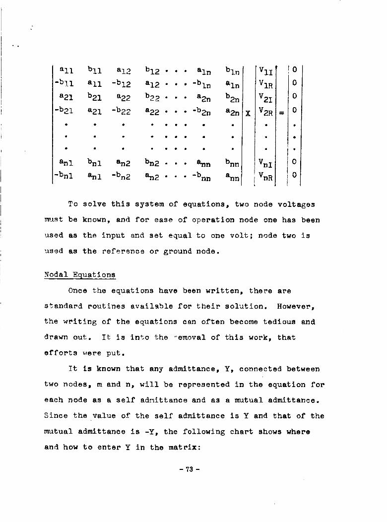
all bll a!2 b12 • . . aln bin

-bll all -b12 a12...-bin aln

a21 b21 a22 b22 • • • a2n b2n

-b21 a21 -b22 a22 • . . -b2n a2n

• • • • • • • • •

anl bnl an2 bn2 • . . ann bnn

-bnl anl -bn2 an2 • . . -bnn ann

VlI

!VIR

V2 I

X V2R

JVnii

IvnR

!0

0

IoI

=I0

I

I"I"

i04io

To solve this system of equations, two node voltages

_l_t be known, and for ease of operation node one has been

used as the input and set equal to one volt; node two is

used as the reference or ground node.

Nodal E_uations

Once the equations have been written, there are

standard routines available for their solution• However,

the writing of the e_lations can often become tedious and

drawn out. It is into the _emoval of this work, that

efforts were put.

It is known that any admittance, Y, connected between

two nodes, m and n, will be represented in the equation for

each node as a self admittance and as a mutual admittance.

Since the value of the self admittance is Y and that of the

mutual admittance is -Y, the following chart shows where

and how to enter Y in the matrix:

- 73 -

_01.ROW_ m

m Y

n -Y

-y

Y

Referring to the real number group, the real and

imaginary parts will be entered in matrix (4) in the

sixteen positions given below:

Col.

Row

2m-I

2m

2n-I

2n

2m-I 2m

a b

-b a

a b

-b a

2n-I 2n

a b

-b a

a b

-b a

(3)

(4)

Voltage Controlled Current Sources

The effect of a voltage controlled current source

upon the matrix can be shown by the following example,

see Fig. 1 •

In writing the equations for the five nodes, the

effect of the source upon the equations can be observed.

- 74-

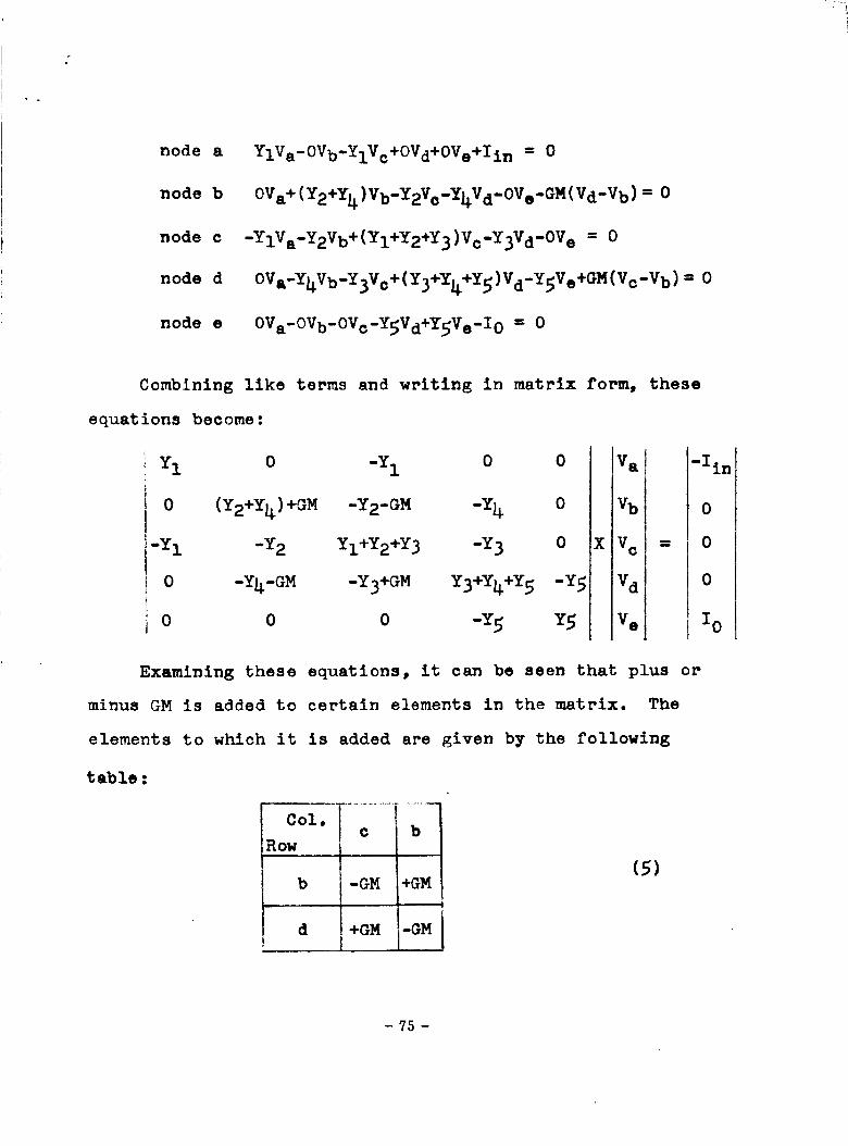
_' i_̧ i_

node a

node b

node c

node d

node e

YlVa-OVb-YlVc+OVd+OVe+lin = 0

0Va+(Y2+Y 4)Vb-Y2Vc-Y4Vd-0Ve-GM(Vd-vb) = 0

-YlVa-Y2Vb + (YI+Y2+Y 3 )Vc-Y3Vd-0V e = 0

OVa-Y4Vb-Y3Vc+(Y3+Y4+Y5)Vd-Y5Ve+GM(Vc-Vb) = 0

OVa-0Vb-OVc-Y5Vd+Y5Ve-I 0 = 0

Combining like terms and writing in matrix form, these

equations become :

fiYI 0 -YI 0 0

i 0 (Y2+Y 4) +GM -Y2-GM "Y4 0

i -Y2 YI+Y2+Y3 0i"YI "Y3

I 0 -Y_-GM "Y3 +GM Y3+Y_+Y5 "Y5

i 0 0 0 "Y5 Y5

X

iVa

Vb

V c

V d

V e

'loin

I °0I Io

Examining these equations, it can be seen that plus or

minus GM is added to certain elements in the matrix. The

elements to which it is added are given by the following

table :

Col.

Row

b

d

-GM

I+GM

I+GM

-GM

(5)

- 75 -

where this means that to Ybb, +GM is added and to Ybc, -GM

is added, etc.

If the notation GMm_pq is adopted to indicate that a

voltage from node m to node n causes a current to flow from

node p to node q, the above source would be given by GMcbbd"

From this and the preceding table, the table can be

written in a general form.

Col.m n

Row

p -GM +GM

q +GM -GM

(6)

Since GM is a real number, when the change is made to

the real number form (see eq. 4), only the real parts are

affected. The additions to the matrix then become:

Col.2m-I 2m 2n-I 2n

Row

2p-I -GM 0 GM 0

2p 0 -GM 0 GM

2q-I GM 0 -GM 0

2q 0 GM 0 -GM

Using these methods, the nodal equations can be

-76 -

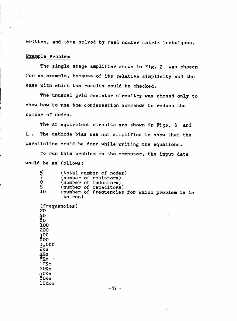
written, and then solved by real number matrix techniques.

Example Problem

The single stage amplifier shown in Fig. 2 was chosen

for an example, because of its relative simplicity and the

ease with which the results could be checked.

The unusual grid resistor circuitry was chosed only to

show how to use the condensation commands to reduce the

number of nodes.

•

The AC equivalent circuits are shown in Figs• 3 and

The cathode bias was not simplified to show that the

paralleling could be done while writing the equations.

To run this problem on the computer, the input data

would be as follows:

570

5I0

(total number of nodes)

(number of resistors)

(number of inductors)(number of capacitors)

(number of frequencies for which problem is tobe run )

(frequencies)2O

100200

I, 0002Kc

10Kc

20Kc

0Kc

100Kc

- 77 -

2I0

1

(number o_ condensations)

(number of passive elements after condensations

are made )

(number of active sources)

(inductances)

(c apacit anc es )IE-06

3.8F-122.8E- 12

IE-12

IF-06

(If there were any inductors, theorder in which the values were read

would indicate the position in

storage, i.e. the first value is

stored as 2,1; the second as 2,2, etc.)

(The first value is stored as 3,1;

the second as 1,2; the third as 1,3,etc. )

(resistances)IE06IE06

5E05IE04

IE03

6.6E03

IE04

(The first value is stored as I,I;

the second as 1,2; the third as 1,3,etc. )

(condensations) (The first number signifies the

operation; i for series combination,2 for parallel combination. The

next four numbers are the locations

in storage of the two elements tobe combined. After the combination

they will be stored in the same place

as the first element, i.e., the first

condensation says to parallel the

elements I,I and 1,2 and put theresults in I,i)

(passive topology)(The first two numbers are the nodes1331

2311

34323533

241_24I2416

34

25i8

between which the element is connected,and the remaining two are the location

of the element in storage, i.e., thefirst group says to put element 3,1

between nodes 1 and 3.)

-78 -

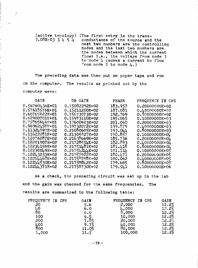
(active topology) (The first entry is the trans-

3.08E-03 3 h 5 4 conductance of the source and thenext two numbers are the controlling

nodes and the last two numbers arethe nodes between which the current

flows i.e., the voltage from node 3

to node 4 causes a current to flowfrom node 5 to node 4.)

The preceding data was then put on paper tape and run

on the computer. The results as printed out by the

computer were:

GAIN

0.56769436E+01

0.576185765+01

0.607650225+010.629007015+01n vC_g<&h6F+01

0.96962458_+01

0.I1324_97E+020.I1622281E+02

0.12076287E+02

0.12201907E+02

0.1223h15_E+02

0.1223_049E+020.12243233E+02

0.]22444685+02

0.122h/_5305+02

0.122h/_371E+02

DB GAIN

0.150822925+02

0.152112505+02

0.15673073E+02

0.159731105+02

0.17600903E+02

0.197320725+02

0.210806655+02

0.21305827E+02

0.21638669E+02

0.21728_54E+020.21751481E+02

0.217542/_E+020.21757922E+02

0.21758798E+02

0.217588h25+02

0.217587305+02

PHASE

183.957

187.o81192.769

195.065201.060

_77._Is

193.044190.857

185.736

182.893

181.418

1 1.1 4180.471i_0.062

179.6_5

179.541

FREQUENCY IN CPS

0.20000000E+02

0._00000005+020.800000005+02

0.I0000000E+03

0.20000000E+03

0 hOO00000E+03O: 60ooo0oE+030.10000000E+0_

0.20000000E+04

o.boooooooE+o40.80000000E+040.I0000000E+05

0.20000000E+05

0._000U000E+050.80000000E+050.I0000000E+06

As a check, the preceding circuit was set up in the lab

and the gain was checked for the same frequencies. The

results are summarized in the following table:

FREQUENCY IN CPS GAIN FREQUES_CY IN CPS GAIN20 5.6 2,000 12.25

6.0 ,ooo 2.256.0 _,000 12.25

100 6.5 I0,000 12.25

200 7.85 20,000 12.25

_ 9.75 _0,000 12.2511.05 _0,000 12.25

1,000 11.5 I00,000 12.25

- ?9 -

From the curves plotted, it can be seen that the

response as calculated by the computer is in agreement with

the experimental data.

The input and computing time for this problem was

fifteen minutes, while it took close to an hour to set up

the circuit and make the required measurements. The savir_g

in time is even greater than it seems because the computer

also calculated phase response while the laboratory

procedure did not.

- 80 -

_ ..i̧_

F,!

i I0f-!

o3

r_

r_0

]

C)

0

Appendix

Actual Program

Implementing the preceding principles a program has been

written for the G.E. Desk Side Computer System (DSCS). The

program can be applied to any network made up of admittances

and voltage controlled current sources with up to seven

nodes. The size limitation is onl_ a factor of memory

space and with a larger memory available could easily be

extended to twenty or more nodes. Two limitations that

have been imposed on the system is that node one be con-

nected only to node three and that the output node have the

highest number.

The first thirty-three statements in the program deal

with putting in the required data. Statement thirty-four

repeats everything that is to follow for each value of

frequency in question.

The next sixteen statements calculate the impedance and

the admittance for all inductors and capacitors for the

frequency in question. If any condensations must be made,

the next twenty-two statements will do the required

calculations. Statements fifty-seven to sixty-three will

combine two elements in series and statements sixty-four to

seventy will combine two elements in parallel.

The next twenty-five statements put the admittances into

- 82 -

their proper place in the Y matrix, following equation (4).

Also included in these statements is the ability to parallel

elements by adding the new admittance to any value that was

previously entered in the same position.

Then following equation (7), the next eighteen statements

add the controlled sources, if any, to the proper places in

the matrix.

Since VII and V2 were defined as zero, all elements from

the first, third and fourth columns and rows disappear.

Also s_nce VIR was defined as one volt, all elements of

column two are constants and can be moved to the other

s_de of th_ equal sign. The remaining matrix must then be

inverted and to do this it was necessary to define a new

matrix YM which does not contain the values from the first

four rows and columns.

The next sixty-three statements write the YM matrix and

then invert it using the Gauss-Jordan Method. [8] After

the matrix has been inverted, it is multiplied by the

constant vector to obtain the output. This is simplified

since it was stipulated that node one must be connected

only to node three and by doing this the constant vector

has only one non-zero member and this has the value of the

admittance between nodes one and two.

After obtaining the magnitude and phase of the output

voltage, the process is repeated for each frequency and

then the entire frequency response is printed out.

- 83 -

Start

IL

data

,l _'

Find Y' s Ifor F l

Ieondens at ions

iPut Y's in

matrix

rI _uto_,__oI[ matrix I

Define YM ]matrix

r

[ Invert YM 1mat fix

i

Calculate !

output

voltages t

..... •

Print response Itable I

Repeat for, each F

- 84 -

References

(i)

(2)

(3)

(4)

(5)

(6)

(7)

(8)

J• McCarthy, "Time-Sharing Computer Systems",

collected in Management and the Computer of

the Future, ed. M. Greenberger, pp. 219-248,M.I.T. Press, 1962.

R• Fano, "The MAC System: the Computer Utility

Approach", IEEE Spectrum, vol. 2, pp. 56-64,January, 1965.

C Strachey, "Time Sharing in Large, Fast Computers"Proc. International Conf. on Information

Processing, UNESCO, Paris• 1960, pp. 336-341.

J.C.R. Licklider, "Man-Machlne Symbiosis" IRE Trans

on Human Factors in Electronics, vol. HE-I,pp. 4-11, March, 1960.

International Business Machines Corp., "IBM 7040/70_QUIKTRAN System Programmer's Guide", File No.7070-25, September _o__. Jvj.

General _lectric Co., "Desk Side Computer SystemReference Manual", April, 1966.

T. Fleetwood, "Automatic Solution of Network FrequencyResponse"• Electronic Engineering, September,1965.

J.M. McCormick and M.G. Salvadori, "Numerical Methods

in Fortran", New Jersey: Prentice-Hall, 1965.

- 85 -

e_ c d e

Zin-'_ .... __ o _ l o

b

FIG. 1

C

O

I Ff _N7IM IM

IOK>

---- 318 V"

500 K I0 K I,u.f

0

:)

FIG. 2

- 86 -

2

FIG. 3

I 5

{,,T ITI o_.._,,k. -, t 1 1Ip.f

3.8 pf _3.08 x I0 6.6 K .L. I pf

Rg IOK

0 _ _ _ 02

FIG. 4

- 87 -

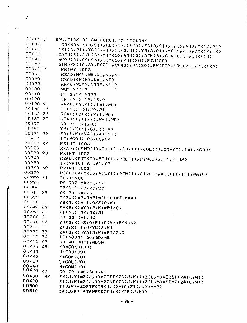
(% t't ?"_( ) f "_

ono;_o

o003o

ooo,ao

nopsn

ono_o

onN7o

ooor_n

finn o,'3

_hql 1i3

r,C_l 30

q Q ] 40

NOI 5{3

O016O

O0 1 70

O01F:O

00100

OnA,Tn

N(72 I _7

0 r,,':_2n

,.3CJ23r3

_0240

OOR50

00A60

00270

00_0

Oq,o_O

nOlO0

0,7._ ! 7

00320

OO3_O

00350

00360

0c,370

• O03FC

0 p, A-_,-',

O_3X.'l 7

Ol_/ |0

00Z430

• 00440OOZ:50

0046000470

00480

00490

00500

00510

47

48

C SqI.UTI.3N elf AN EI.F.CT_-.'IC X!_'Tb;ORR

C q.vj:'40 N Z(3,21 ), A1.(20),C(20), ZA(3, 21 ), Zi_('3, 21 ),Y( 1 4,P 1 )

tZI(3,PI),YA(3,21)sYI(3,21),YR(3,fil),YB(3,_I),YM(I_, 14)

3AG"I(5), A]L( 5),AT4( 5),ATN( 5),ATK(5),CONT( !0) ,CO_<(10)

4C,q..l( 5), COl.( 5),COM( 5),PTI (20),PTJ(20)

5I NDEX( 10, 3) ,F(_O) , V(20), C--A(20)sPH(20) sPTI. (20) ,PTM(?O)

7 PRINT 1003

REAl]: NAM, NR, NL, NC, NF

READ: (F(N) ,N=I ,NF)

_EAO: NCON, NTOP,,N_ | q

NUVI=NAH*2

PI=3,1 4159.0-7

IF (NI.) I 5, 15,9

9 READ: (AI.( T ), I =1 , IX'l. )

15 IF(_C) 20,20,21

21 READ: (CC_) ,I<= 1, NO)

20 E:EAD:(Z(I,K),K=i,X'F<)

Dq ,05 '<=I,NR

Y_( I,:<)=I 00/Z( 1 ,_<)

25 ZA( I•_()=YA( 1, _()=0. Q

I F(._CON) 23,23,24

24 PRINT 1003

READ: (CON'9(I),GO.J(I),CONCI),COLfI)sC'.'3ffCI), I=I,NCON)

23 PRINT 1003

READ:(PTI(I)sPTI(1),PTL(I)sPTM(1),I=I,v]3P)

I FfNATO) 61,61,62.

62 PRINT 1003

READ: (AGM(I)• ATL( I)sATM( I ),ATN( I ),ATK( I ), I =1 ,NATO)

61 CONTINUE

DO 792 MAK=I,NF

I FCNL) 28,28,29

29 Of) 27 !<=IsNI..Z (2, K) =2 °O*PI*AL('.C)*F(MAR)

YBC2, K) =- I -O/Zfe, K)

27 ZA(2sK) =YA(2, K)-PI t2.

q2: IFCNC) 34,34,31

31 Or) 33 _(=I,NC

32 YB( 3, K) =2 .O*P I*C(K) '_F(_4AK)

Z(3,K)-I .O/YB(3,K)

33 ZP (3, g) =YA(3, K)-PI t2.0

34 I F(NC_N) 60,60,42

42 !30 40 .JO=1sNCON

45 NO=CONO (30)

l=COJ(JO)

K=COK(.JO)

L=C_I., (.10)

M=Cf)M(JO)

GO TO (4R,SS),NO

ZR(J, K) =Z (.J,g)*COSF(ZA(.J, K) )+Z (t, M) w,COSF(ZA (L, M) )

ZI (.J, K) =Z (.Jsg) *SI NF( ZA( J, K) )+Z(L, M)eSINF(ZA(L,M) )

Z (.is g) =SQRTF( ZR(J, g )**_.+Z I (J, g)**2)

ZA(.JsK)-ATANF(ZI (J, K)/ZR(J, K) ))

- 88 -

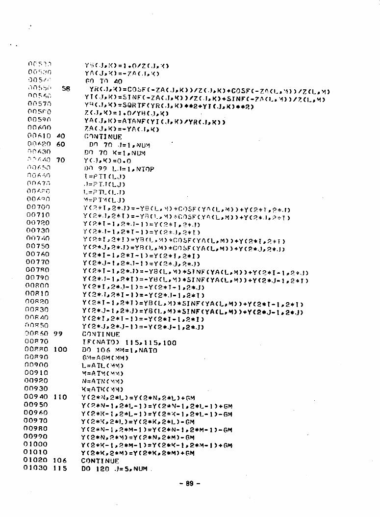
NC'5:2.'_O0 53Q

<]05z<:

O0. 57-_

OC)5rO

OOSq_

006,q0

00610

00 _20

n0_,30

,'3,0 _ 4q

00 f,"_ tq

O0 70_]

00710

007_0

00730

O0740

00750

00760

00770

O0720

00790

OOSO0

00_I0

O0220

00_30

6)OR 4r)

r.r)R50

00R_O

00270

OOP_O

OOR�O

O0900

00910

00920

00930

00940

009 50

00960

00970

00920

00990

01000

01010

01020

01030

58

aO

60

7O

99

I00

II0

I06

115

Y;:+(.J, I'C) = I -O/Z ('.I, "<)

y .fx.(J, _<) =- 7./_ (. h, _)

G+3 Tt3 Z_O

YRC.J,;()=C05F(-ZA(J,K) )/Z(.}JR)+C03F(-Z_ eL,'1) )/Z(L_ M)

YI (.],K)=SI NF(-ZA(J,K) )/Z(.I, K)÷SINF(-Z/_(L, M) )/ZfL,M)

Yq(3, K) =S(_RTF(YR(.I, l<) _*2+YI (3, K)e_)

Z (.+J,K)= I .0/Y13 (.J, I()

YA(.J,K)=ATANF(YI (.!, R)IYR(.I,R) )

ZA (,J, K) =-YPt(.Y, _()

CqNTINUE

Dr_ 70 .J=I,NUM

Dr) 70 K:I,NUM

Y( ],K)=O.O

Dq 99 L.I=I,NTOP

l =PTI (L J)

.I=?T.I(LJ)

I.=? TL (I,.I)

"q=P 1""4( L.] )

Y (2" I, 2*.J) =-YB (L, '.I)*COSF (Y,'_(L, _) ) +Y (2. I, _*.I)

Y (2..l, 2. I ) :-Y_ (i.,"_)*6")_%F (Yh (L, M) ) ÷Y(2*.}, _:._¢I)

Y(R*I- I • 2".I- ! ):Y(2*I, 2..I)

Y(2*.I- 1,2"I- ! ):Y(2*.J, 2.[ )

Y,'_*I,2*! )--YB(L:,'4) *COSF(YA(L,M) )*Y(2*I,2*I )

Y (2*J, 2..9) =YB (L,.M) *COSF(YA (L, M) )+Y (2..], 2*J)

Y (2.I- I, 2.I- 1 ) =Y (2. I, 2.I )

Y (2*J- 1 • 2*J- 1 )=Y (2* J, 2..])

Y (2.I- I, 2*J) =-YB (L, '4)*LI NF(YA (t, M) ) ÷Y (2"I- I,2*.9)

Y(2*.I- I,P_*I )--YB(L,M)*SINF(YA(L,M) )÷Y(2*J-1,2.I )

Y(2*I,2*J-1 ):-Y(2*I- I,2*J)

Y(2..I,2.I-! )=-y(2.-wJ-1 ,R*I )

Y(2*I- 1,2*I)=YB(L,_)*SINF(YA(L,M) )÷Y(_*I- 1,2.I)

Y (2*J- 1,2*.])=YB (L, M).5I NF(YA(L, M) )+Y(_eJ-1 ,.2*J)

Y(2*I,2*I-! )=-Y(2*I- 1,2.I )

Y (2*.J, 2*.J- 1 )=-Y (2*.J- 1,2*.J)CC)NTI NUE

I FfNAT0) 115,115,100

D0 106 =_M=I,NATO

Gg:AGM(MM)

L=ATL(MM)

Y(2*_,2*I,)=Y(

Y(2*N-I,2*L-I

Y(2*IK-I,2*L-I

Y(2*!(,2*L)=Y(

Y(2*N-I,2*M-|

Y(2*N,2*M):Y(

Y(2*K-I,2*M-I

Y(2*K,2*M)=Y(

CONTINUE

DO |_0 ,I:5, NUM

2*N,2eL)+GH

)=Y(2*N-I,2*L-I)+GM

)=Y(2*X-I,2*L-I)-GM

2*K,2*I.)-GM

)=Y(2*N-I,2*M-|)-GM

2*N,2*M)-GM

)=Y(2*K-I,_*_-I)÷GM

2*K,2*M)÷GM

- 89 -

01040

01050 120

D.") 120 K=5, NU:'!

¥'d(J- A, K- 4)=Y(.I, K)

Onooo c

ooo 17,

00020 125

0003_ 135

oooL(-) 145

00050 155

0(_060 165

00070 1 75

0,'_ 09,n l,g5

001 O0

OG110 195

OOtqO .?.15

0¢11.3r_ .925

OC, 1 z,q

OG 1 50 205

QC, 16,0 180

00170

O0iqO 260

00190 2.70

os.'__-.no 130

0)') "_1 ('_1400099.0 150

7:q.'7".30 160

0C, 2/C, 170

00250 200

00260 310

00270

002_0 330

00290 340

00300 350

00310 3_0

003.':_.7 390

O02.'_0 40000340 420

00350 430

00360 450

00370 550

O03RO 600

00390 610

00400 620

00410 630

00420 640

00430 650

00_40 660

00450 670

00460 700

SOLUTION OF AN ELECTRIC NETWORK(PART TVO)

N=NUH- 4

13FITEF'M= I *0

I3G 145 .J=laN

INDEX (..h.3) =0-0

DO 550 I=I,N

AMAX=O*O

DO 180 J=I,N

IF(INDEX(,;, 3)-1 ) I._35,IIXO, 71 5

DO _05 ,"(=I,N

IF(INDEX(K, 3)-I )195,205, 715

IF(#_d.aX-ABSF(Y<'(.J,V,))) P_15, 20 5. 20 5

I v.'Ot','=,l

I COL UM='(

A_4AX=ABSF (Y"4( .1, '<) )CONTINUE

CONTINUE

INDEX (IOOLU:4, 3) =I NDEX (ICOLUH, 3)+I

INDFLK (I, I ) =I F:O_:2

INDEX(I,2) =ICOLUM

I F(I ROk'- I COLUM) 140,310,140

DETERM=-DETERM

DO 200 L=I,N

S k:AP=YM ( IRO W, L )

Y'4 ( I}'_0W, L )=YM( I COLUM, L)

Yi'1(ICOLUM, L )=SWAP

£ I VO T=Y-"I( ICOL U.'4,ICOLUM)

DETERH=DETERH*P I VOT

YH(ICOLU_, ICOLUH}=I -0

DO 350 L=I,N

YH(ICOLUH,L)=YM(ICOLUM, L)/PI VOT

DO 550 LI=I,N

I F(LI -ICOLUM) 400, 550,400

T=YM(LI, ICOLUM)

YMCLI, ICOLUM)=O*O

DO 450 L=I*N

YMtL I,L )=YMCL I,L)-YM(ICOL UM,L)*T

CONTINUE

DO 710 I=I*N

L=N+I -I

IF(INDEX(L, 1)-INDEX(L,2))

JROW: INDEX(L, I )

JCOL U;'I=I N D F..X( L, 2 )

DO 705 K=I,NS WAP=YM (K. JRO W)

YM (1(, JRO W) = YM ( K, JCOL UM )

YM( K, JCOL UM) -SWAP

630,710) 630

- 90 -

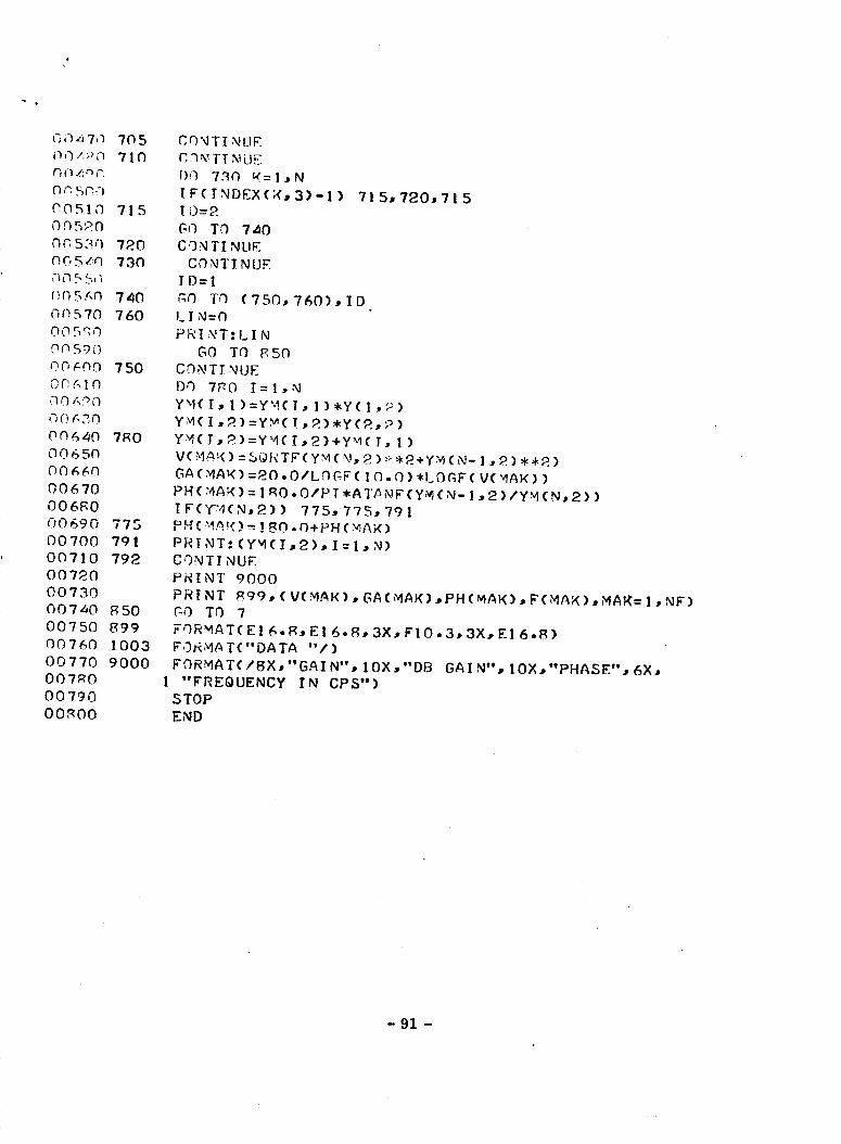
(]()n 7,]

0,3 A:c'O

nn 5c..h

O0510

ON 5_0

OC_ 530

OOSz_n

f'.,(]5 ,_,_

00. 570

O05qO

Oo 590

OC, _OQ

OO.AIO

qq Ag,q

0 C'_SO

00640

00650

O06;&0

00670

OOSgO

00690

00700

00710

00720

00730

007_0

0O75O

00760

00770

007_0

00790

O0SO0

705

710

715

72.0

730

740

760

75O

780

775

791

792

S50

899

1003

900O

CONTINUE

I)O 730 W=I,N

TFC INDEX(;(, 3)-I) 71 5,720,71 5

[0=2

GO TD 7_0

C.gN TI NLIK

CONTINUE

II)=l

GO T_ (750,760),ID

LIN=Q

PRI_T:LIN

GO TO _50

CONTINUE

DO 7_0 I=I,N

Y"I(I, I)=YM(I, I)*Y(I,,2)

Y_( I, 2 ) =YY( I, 2)*Y (2, P)

Y_(I,2)=Y_'4(I,2)+Y_(I, 1)

V( MA!( ) = SO;<TF (YM ( _l,"_2.)_ :_2 +Y:.i(N- I• 2 ) • _-2)

GA(MA_() =20.O/LOGF( 10. 0) %I_OGF(V(MAK) )

PH('4AK)= 1R0.O/PIeATANF(YM(N- 1.2)/YM(N,2) )

I FCY?4(N,2)) 775,775, 79l

bue ,,,Iale'_.=_IRn Q+PH (MAK)

PRINT: (YMCI _2) _ I=I, N)

CONTINUE

PR! NT 9000

PRINT R99, (VCMAK), GACMAK),PH('MAK), F(MAX),MA_(= l ,NF)

GO TO 7

FORMAT(El _.R, E! 6. g, 3X, FI O. 3.. 3X, El 6-8)

FORMATC"DATA "/)

FORMAT(/BX,"GAIN",IOX,"DB GAIN",IOX,"PHASE"*6X*

I "FREQUENCY IN CPS")

STOP

END

- 91 -

Section V. On the Accuracy of Monte Carlo Method

It is generally recognized that in order to get

meaningful answers from Monte Carlo simulation it is

necessary to run the " experiment" a great number of times,

varying from run to run only the particular random numbers in

generating the combination of parameter values, to provide a

large sample typical of the system.

The Automated Statistical Analysis Program [I_ developed

by IBM for circuit analysis, for example, uses I0,000 as the

standard setting for the number of cases to be tested. In

asce_talnir_ the adequacy of this number of runs there are

two extremes to be kept in mind. Cursory computation on one

hand imparts little significance to the results to be useful

in assessing the true performance of the circuit under

investigation. On the other hand, exhaustive testing, even

if it would not exceed the capability of the computer

facilities available, defeats the purpose of random sampling

which attempts at conclusive results from random selection of

sample points. It is to be noted, however, that the accuracy

of the statistical method actually bears a nonlinear relation-

ship with the number of runs in the test. The intuitive idea

that the more times the computation is carried through, the

more meaningful the result will be, is often a vague and

sometimes misleading notion.

- 92 -

The accuracy of the Monte Carlo method mainly depends

upon two factors: the number of runs and the randomness of

the random numbers to be used in the tests. Take the

instance of finding the area of an irregular geometric figure

by the Monte Carlo method. First, draw the figure on a piece

of paper of known dimension and therefore known area, put

your finger down at random. Possible outcomes will be (a)

the finger will land inside the irregular f_gure, a "success";

(b) it will be outside the figure, a "failure"; (c) it will

come down on the boundary of the area or it may miss the paper

entirely. After a large number of trials and ignoring the

outcome of (c), the unknown area can be estimated by mul-

tiplying the total area of the paper divided by the sum of

the number of successes and failures. The accuracy of the

answer depends upon two factors. First, the number of

trials must be large; second, the finger must be put down

in a random manner each time.

Pursued by hand, the Monte Carlo method will only lead

to bruised thumbs and poor estimates of the area. Mechanical

means can be used to provide random numbers which tell the

machine how to "put its finger down". But the wear of

mechanical parts will develop a bias in favor of a particular

number. With the advent of electronic digital computers,

this situation is relieved; and we shall be able to approach

randomness as nearly as allowed by the scheme we can devise.

- 93 -

In this section, the accuracy of the Monte Carlo method

and some of its main characteristics will be discussed. An

exposition on the generation of random numbers will be

presented in Section VI.

Bernoulli' s Theorem

In the theory of probability one of the most important

and beautiful theorems was discovered by Bernoulli (165J,-

1705) and published with a proof remarkably rigorous in his

admirable posthumous book " Ars ConJectandi" (1713). If, in

n trials, an event E occurs m times, the number m is called

the " frequency" of E in n trials, and the ratio m/n receives

the name of " relative frequency" . Bernoulli's Theorem

reveals an important porbability relation between the

relative frequency of E and its probability p. It may be

stated as follows: with the probability approaching I or

certainty as near as we olease, we may expect that the

relative frequency (m/n) of an event E in a series of

independent trials with constant probability p will differ

from that probability by less than any given number 8 • O,

provided the number of trials is taken sufficiently large.

In other words, given two positive numbers 6 and a, the

probability P of the Inequality

m Pl >8 (1)

- 94-

w__ll be greater than 1 - a if the number of trials is above

a certain limit depending upon 6 and a.

To illustrate Bernoull_'s Theorem, Uspensky [21 has

given the example that, if p = 1/2, 6 = .O1, a = .001, the

formula

n >_ 1 + 6 In 1 + 1 = 69,86962 a 8

(2)

shows that in 69,869 tr_sls or more there are at least 999

chances against 1 that the relative frequency will differ

from 1/2 by less than 1/lO0. The number 69,869 found as a

lower limit of the number of trials is much too large. A

much smaller number of trials would suffice to fulfill all

the requirements. From a practical standpoint, it is

important to f_nd as low a limit as possible for the necessary

number of trials (given 6 and a).

Since p is the required quantity while m/n is the ap-

proximate value obtained by the Monte Carlo method, it

mfollows that the difference _ - p is the error of the Monte

Carlo method. It is clear from the above that this error may

be estimated probabilistically with a degree of reliability

I - a.

The Limit Theorem in the Bernoulli' s Case

The concept of Bernoulli trials, which deals with

- 95 -

experiments having only two possible outcomes, is extremely

useful because we are often interested only whether a certain

result occurs among many possible outcomes or not. For

example, although the output voltage of an electric circuit

may assume a range of possible values, we are concerned only

with whether it exceeds a specified value or not. By

Bernoulli's Theorem it is Justified to use the ratio of the

number of successes m to the total number of trials n, m/n,

as an estimate of the binomial probability of success, p.

The number of successes chsnges from one binomial experiment

of size n to another. It is thus a random variable, wblcb

will be designated as M, with possible values m = O, I, 2 . . .

n. Since M is a random variable, so is _ = m, with possible

values O, l/n, 2/n, . . . (n-l)/n, I.

The statistical averages of the random variables M and

A

p are:

E(M) = np

Vat(M) = npq _M =

E(_) = E(_-) = In E(M) = p

M 1 PAVar(_) = Var (_) = _z Var(M) = n

P

(3)

(5)

(6)

where q = l-p. A comparison of equations (l!) and (6) reveals

the interesting fact that _M imcreases as n increases for

fixed p, while _ decreases as n increases. If the variance

is small, then the value of the random variable tends to be

- 96 -

close to its mean, which in this case (so called " unbiased

estimate" ) means close to the true value of the parameter

_n question.

There are two approsches to f_nd more precisely the

relationship between the size of the sample, n, and the

error of _ in the estimation of p, 16 - P_.

I. Conservatlve Chebyshev Approach

The well-known inequality bearing the name of the

Russian mathematician Chebyshev (1821-189_) gives the upper

(or lower) bound of such probabilities P [IX- E(X)I< C ]when

E(X) = _ and Vat(X) = _2 are given. It may be stated as

follows: for any positive number C,

(7)

This means that the probability assigned to values of X

outside the interval _ - h_ to _ + h_ is at most I/h a . In

other words, at least the fraction I - (I/h a ) of the total

probability of a random variable lies within h standard

deviation of the mean.

In applying the Chebyshev inequality with _ = p and

= _ in the case at hand, we find the probability that

p is within h _ of p is at least I - (I/h a ). One

difficulty is that _ is dependent upon the exact value of p

A

which is to be estimated by p. However, we can find the

- 97 -

value of p that ,mximizes _z = pq/n. Since the graph of

pq = p(1 - p) is a parabola that is symmetrical about the

llne of p = 1/2, the maximum value of pq is attained when

p = q = 1/2. Therefore, the maximum value of pq is

I/2" 112= II_,and

Therefore we can say conservatively that the probability

is at least I - (I/h s) with the distance

l_.pl < h__(B)

For example, if n = 1,O00 and if we choose h = 2, the

probability is at least 0.75 that

l_'- pl '_ 2 = .032- _v_,ooo

or, in words, at least 75% of the probability distribution

of p is within .032 of p. For n = 1,O00 and h = 5, at least

96% of the probability distribution of the error is less than

5/,V_ _ .065.

It is clear from equation (8) that the error in the

approximate solution of a problem by the Monte Carlo method

can be reduced by increasing the number of trials n, i.e. by

increasing the commutational time. For example, the time

necessary to complete the solution must be _ncreased by a

- 9B -

factor of lO0 if the accuracy is to be improved by one order

of magnitude.

2. Conservative Normal Arproach

From DeMolore-Laplace Theorem [ 3 ] in the theory of

probability, it is known that when the mean value _ is " far"

from 0 and n, the extreme values of the binomial random

variable X, (at least 3_ from both 0 and n), it is justified

to use the stronger normal distribution theory instead of the

Chebyshev Theorem. In our case then, If np is at least n3V_

from both 0 and n, we know that the new random variable

Z = (X - np)/v_-q is approximately normally distributed.

Recalling that _ = _, we have

X A

z =x- nP = H "p = P__Z_P__

Now, since Z is approximately distributed according to the

standard normal distribution, we can say that the probability

is approximately 0.95 that

A

-2 < Z < 2 or -2 _ P - P _ 2. (9)

where the Z's represent 2 standard deviations, to approximate

the more precise value 1.96 from the normal table _1.

We now multiply all terms of the right-hand expression

- 99 -

of the inequslity (9) by ,_q-/_, and _e_

Max_mlzin_ pq as before at pq = !_, we find from the normal

distribution that the probability is approximately 0.95 snd

1 _pl < 2 _ i__-

If we choose h standard deviations instead of 2, the

appropriate probability should be obteined from the normal

table.

In general, the number of runs (n) required in the

Monte Carlo method can thus be determined on the basis of

normal distrib_tion approach by the simple relation

Cn -

4E*

where E is the tolerable error range in per cent and

C is the square of probability value for a given confidence

limit.

For example, for 90 per cent confidence limit, C has

the value of (1.64) = 2.69; for 95 confidence limit,

C = (1.96) = 3.84; for 99 per cent confidence limit,

- i00 -

C = (2.57) =6.61. If we want the simulation result to

be within + .05 error range, the number of runs correspond-

ing to the three confidence limits would be 269, 384 and

661 respectively. Returning to the figure given in the ASAP

operating manual, a lO,000-run computation w_ll guarantee

the result to be within + .013 error range with 99 per cent

confidence limit, or, alternatively, + .02 error range with

c9.99 per cent confidence limit.

- i01 -

References

(i)

(2)

(3)

International Business Machines Corp., "ASAP, An

Automated Statistical Analysis Program", Tech.

Rept. prepared for NASA Goddard Space Flight

Center, Greenbelt, Md., Contract No. NAS 5-3373.

J.V. Uspensky, "Introduction to Mathematical

Probability", McGraw-Hill Book Co., 1937, p. I01.

F. Parzen, "Modern Probability Theory and Its

Applications", p. 239; Wiley and Sons, 1960.

M. Abramowitz and I.A. Stegun, "Handbook of MathematicalFunctions", Bational Bureau of Standards, Applied

Mathematics Series AMS-55; U.S. Government

Printing Office, Washington, D.C., p. 968.

- 102 -

Section VI. Generation of Ran4om Numbers on

IBM 1620 Computer*

*This is part of a thesis submitted by J.J. Perkowski inpartial fulfillment of the requirements for the M.S.

Degree to the Electrical Engineering Faculty of VillanovaUniversity, June, 1966.

- i03 -

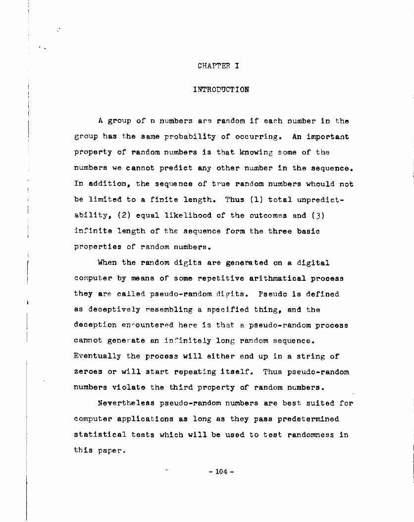
CHAPTE_ I

INTRODUCTION

A group of n numbers are random if each number in the

group has the same probability of occurring. An important

property of random numbers is that knowing some of the

numbers we cannot predict any other number in the sequence.

In addition, the sequence of true random numbers whould not

be limited to a finite length. Thus (1) total unpredict-

ability, (2) equal likelihood of the outcomes and (3)

infinite length of the sequence form the three basic

properties of random numbers.

When the random digits are generated on a digital

computer by means of some repetitive arithmatical process

they are called pseudo-random digits. Pseudo is defined

as deceptively resembling a specified thing, and the

deception encountered here is that a pseudo-random process

cannot gene_ate an infinitely long random sequence.

Eventually the process will either end up in a string of

zeroes or will start repeating itself. Thus pseudo-random

numbers violate the third property of random numbers.

Nevertheless pseudo-random numbers are best suited for

computer applications as long as they pass predetermined

statistical tests which will be used to test randomness in

this paper.

- 104 -

°

Let us consider some of the methods availabl_ for generating

pseudo-random numbers:

A. Von Neumann's Center Squaring Method 6, ]2

Running through the actual procedure of this method _ives a

hint of what can be expected in these random processes.

Proceed as follows :

I) Start with some large number ao containing 2k digits;

azy nuH?uer will do.

2) Square ao to get ao containing 4k digits.

3) Take the middle 2k digits of ao add call this al, the

next random number.

h) a! is then squared and the process continues.

The ass_mpt_on in this method is that any digit is as

likely to occur as any other so the numbers will be random.

Let us see if this is true with some examples.

Example 1

I) Let ao = 1234, number of digits = 2k = 4

2) ao = 01522756, 4k = 8

3) The middle 4 digits are 5227 so aI = 5227

This seems perfectly legitimate but certain numbers do not

work so well.

Example 2

Let ao = 64 then ao = 4096 aI = 09 aI = 0081

a 2 = 09 aI - 0081

a 3 = 06 a3 = 0036

a 5 = O0 -105-

a2 = 08 a2 = 006h

a4 = 03 a4 = ooo9

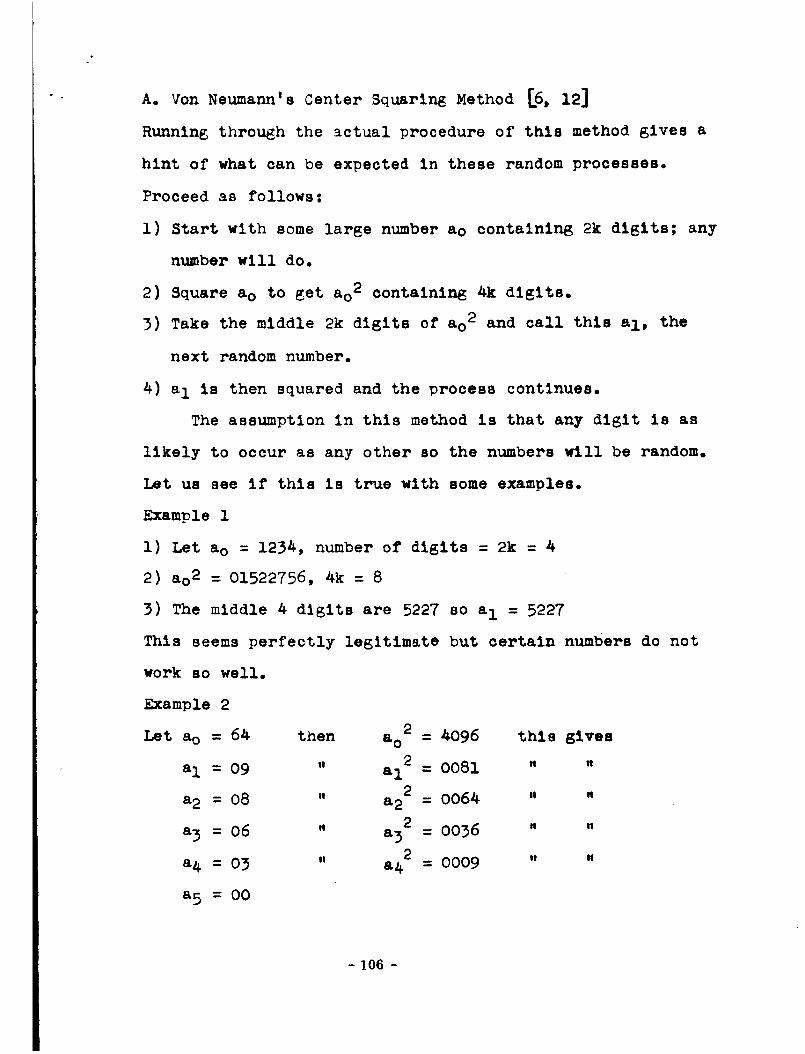
A. Von Neumann's Center Squaring Method [6, 12]

Runnin 6 through the actual procedure of this method gives a

hint of what can be expected in these random processes.

Proceed as follows:

i) Start with some large number ao contalnin6 2k digits; any

number will do.

2) Square ao to get ao 2 containing 4k digits.

3) Take the middle 2k digits of ao 2 and call this al, the

next random number.

4) aI is then squared and the Drocess continues.

The assumption in this method is that any digit is as

likely to occur as any other so the numbers will be random.

Let us see if this is true with some examples.

Example 1

i) Let ao = 1234, number of digits = 2k = 4

2) ao 2 = O1522756, 4k = 8

3) The middle 4 digits are 5227 so aI = 5227

This seems perfectly legitimate but certain numbers do not

work so well.

Example 2

2Let ao = 6A then a o

aI = 09 " al 2

2a2 = 08 " a 2

a3 = 06 " a32

a4 = 03 " a42

a 5 = OO

= 4096 this given

= O081 " "

= 0064 " "

= 0036 " "

= 0009 " "

- 106 -

o

This process degenerates into a string of zeroes for

ao = 64 and for many other values. In addition this method

often degenerates into short cycles of two or three numoers.

Obviously this is not a good method and experience has

shown unsatisfactory results if ao has less than eight

digits. The National Bureau of Standards tried this method

[6] and produced sixteen programs ranging in length from

II to IOA numbers of four digits each with an average length

of 52. This is not very ideal for oractical applications.

B. 16odlfied Yon Neumann Method [6]

Considerable better results are obtained by a modified

version of Von Neumann's method, in which a pair of numbers,

a o and al, are multiplied together and the central digits

of the Droduct are used for the number a 2. The process

is repeated for a I and a2 to give a3. So if a o x aI =

(1234) x (5678) = 07006652 then a 2 = 0066. This type of

process gives _seudo-random numbers that are more random

and with a larger _eriod than the mid-square method. In

the tests run by N?S, ten sequences were comouted, all of

which degenerated into a string of _eroes. The lengths of

the sequences ran_ed from 19 to 1253 with an average length

of 591.

This method will be used later in the com_uter to gen-

erate data.

To summarize:

- 107 -

1) Select a o and al; any 2k digit number will do.

2) Take the product of a o and al; 4k digits.

5) Take the middle 2k digits of this product and call this a 2

4) Take the product of a I and a2 to 6et a3 etc.

C. IBM Method

Thls method was taken from the IBM reference manual [i] and

wlll be used later on the oom_uter. The basic formula for

this Drocess is:

Un+ 1 = last d dlglts of xu n (1.1)

This will produce 5t10 d-2 terms before repeating (for d

greater than 3). An outline of this method as dictated in

the IBM reference manual follows:

I) Choose for a startln6 value any integer u o not dlvlslble

by 2 or 5; Uo ls d digits long.

2) Choose t for equation 1.2 as any integer

3) Choose r for equation 1.2 as any of the values 3, ii, 13, 19,

21, 27, 29, 37, 53, 59, 61, 67, 69, 77, 83, and 91.

_) Take the values from 2) and 3) and choose as a constant

multiplier an integer x of the forth:

x = ROOt __ r (1.2)

(The plus-mlnus slgn is used because x must be odd and odd

numbers have the foz_ 2n + i, 2n _ 3, etc. ; the plus-mlnus

si_ simplifies selectln6 a value close to i0 d/2 as a

choice for x. )

5) Compute XUo, a product 2d digits long

- 108 -

6) Discard the hish order d dlglts leaving u I conslstln6 of

the last d digit of the product.

7) The process is reDeatedo

As an example let d = 4 and uO = 2357. Since IO d/2 = 100

a good choice for x is 109. So xu o = (O109) (2357) =

00256913. Then uI = 6913, xu I = (O109) (6913) = 0O753517

so u 2 = 3517o This method w111 be studied in much further

detail in later discussions.

D. Lehmer Method

D. H. Lehmer is an important name in random numbers and a

very simple method [7] which he developed calls for successive

multiplications b_ a constant number (he chooses 23):

l) Choose an elgght digit number Uo; any number will do.

2) Multiply uo by 23 to 6et a nine or ten digit Uo'.

3) The first and second digits on the left are removed and

subtracted from what remains of uo' 61vlng u1

4) Continue the process with 23u 1

Example

l) uo = 12345678

2) 23u o = 0283950594

3) u I = 83950594-02 = 83950592

4) 23u I = etc.

This method supposedly does not repeat until 5,882,352

sequences have been computed which contains about 47 million

random digits. And so this paper will contain a method similar

109 -

to this that _roduces sequences of six digits each. The

method was modified slightly to better fit the Fortran

comouter lar_uage.

E. Residue Method

In these four methods discussed so far, instructions state

to choose any initial value for u 0 or ao etc. But when

lookln_ at the results of these methods, it will be seen that

only certain initial values give good long programs; the others

_Ive short deteriorating programs. Just what the proper initial

value is, though, can only be determined by trying many dif-

ferent values and selectlnE the best by observing the results.

This, of course, entails a lot of guess work and a good bit

of comDuter hours. And so a method is needed in which one

does not have to _ick a special initial value in order to get

long sequences of usuable numbers. Such a method is the power

residue method [8] which is extensively used today by anyone

wishing to Eenerate random numbers. The IBM manual spells out

the procedure for this method. The method is based on the

equation:

Un+ I = xu n (mod IOa) _1.3)

The procedure i8:

l) 1od represents the word size of the machine and this will

produce 5-10 d-2 terms before repeating. So in order to

have at least 5,000 terms let d = 5.

2) The value of x is arrived at from the congruence

- 110 -

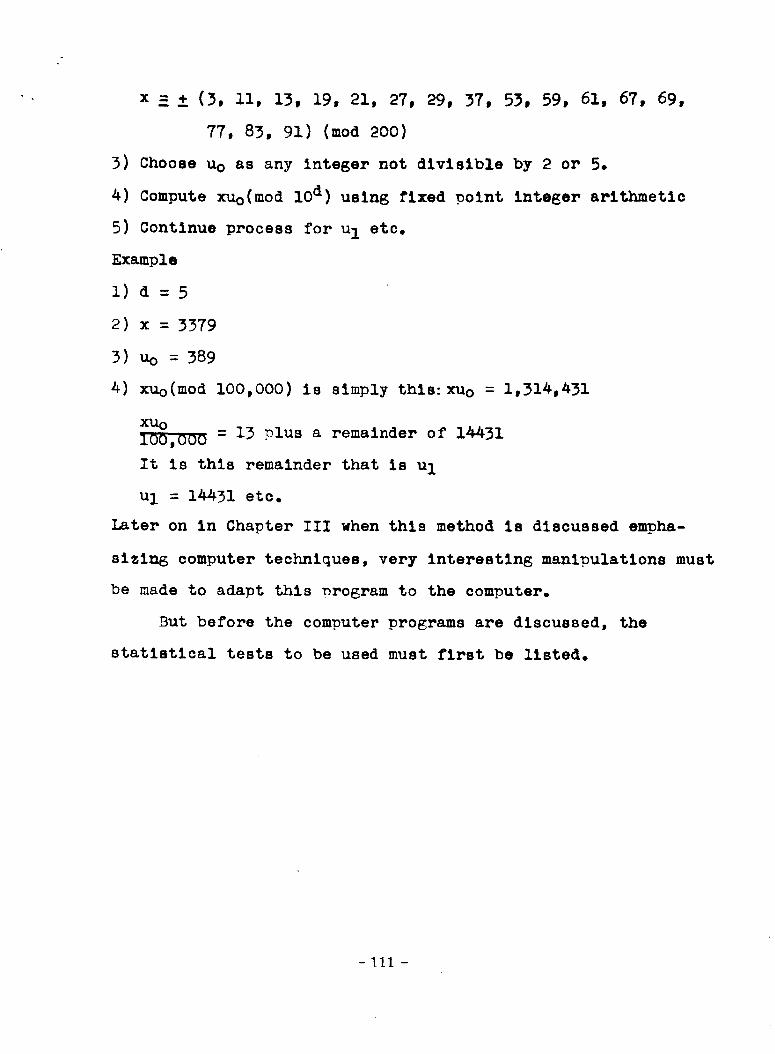
X H _ (3, ii, 13, 19, 21, 27, 29, 37, 53, 59, 61, 67, 69,

77, 83, 91) (mod 200)

3) Choose u0 as any integer not divisible by 2 or 5.

4) Compute XUo(mod I0 d) uslns fixed point Integer arithmetic

5) Continue process for u I etc.

Example

I) d = 5

2) x = 3379

3) Uo = 389

4) xuo(mod lO0,O00) is simply thls:XUo = 1,314,431

XU o

= 13 plus a remainder of 14431

It is this remainder that is u1

uI = 14431 etc.

Later on in Chapter III when this method is discussed empha-

sizing computer techniques, very interesting manipulations must

be made to adapt this _rogram to the computer.

But before the computer programs are discussed, the

statistical tests to be used must first be listed.

- 111 -

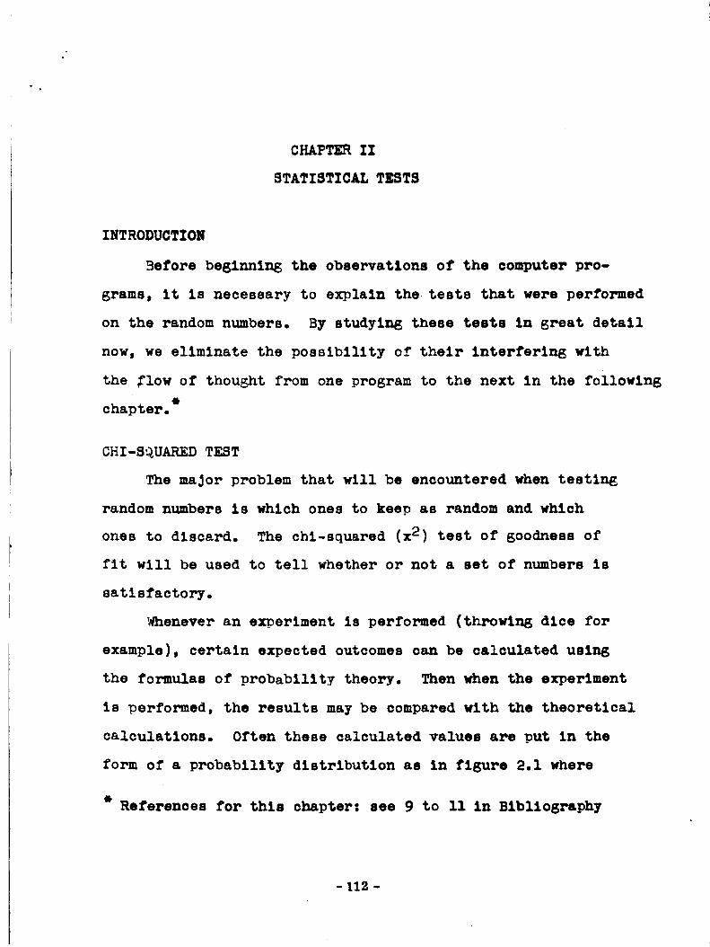
CHAPTER IX

STATISTICAL TESTS

INTRODUCTION

Before be61nnln6 the observations of the computer pro-

grams, it is necessary to explain the tests that were performed

on the random numbers. By studyln6 these tests In great detail

now, we eliminate the possibility of their interfering with

the _low of thou_t from one program to the next in the following

echapter.

CHI-S_UARED TEST

The major problem that will be encountered when testln6

random numbers is which ones to keep as random and which

ones to discard. The chi-squared (x 2) test of goodness of

fit will be used to tell whether or not a set of numbers is

satisfactory.

'Xhenever an experiment is performed (throwing dlce for

example), certain expected outcomes can be calculated usln5

the formulas of probability theory. Then when the experiment

is performed, the results may be compared with the theoretical

calculations. Often these calculated values are put in the

form of a probability distribution as In figure 2.1 where

References for thls chapter: see 9 to II In Blbllography

- 112 -

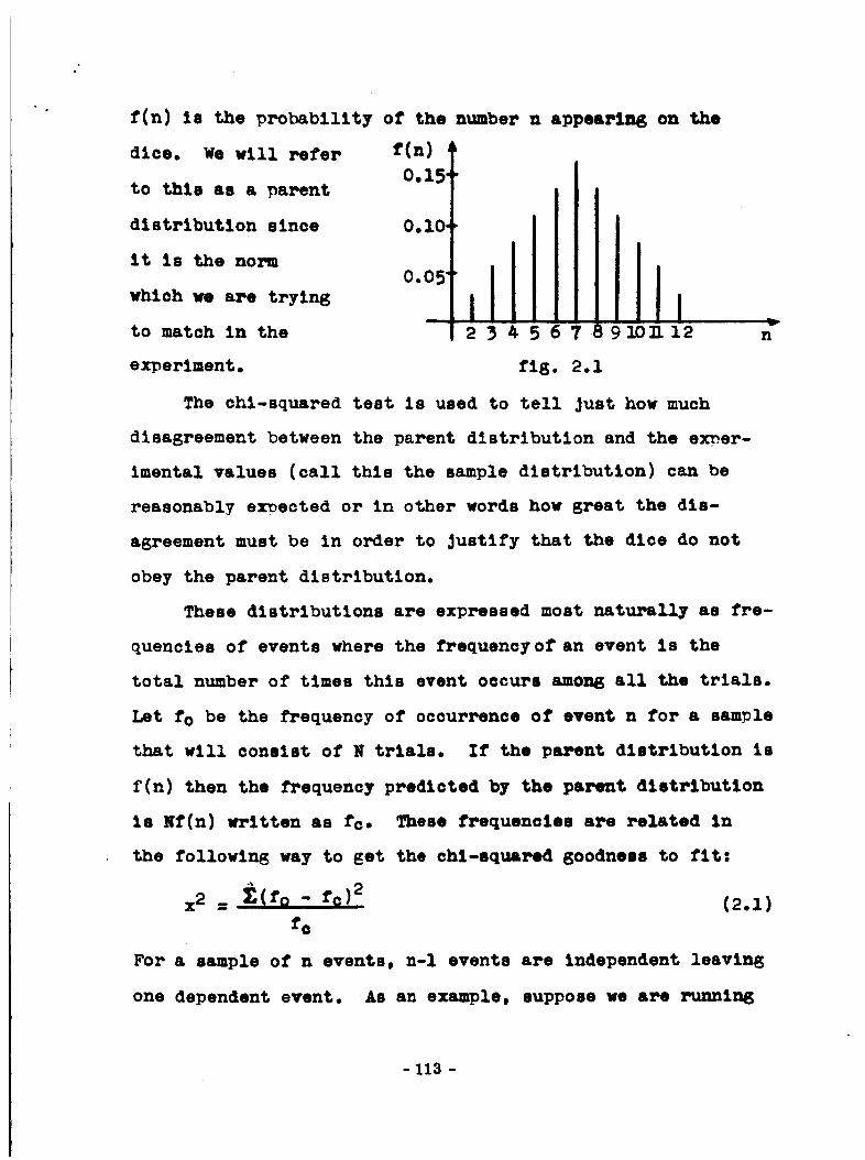
f(n) ls the probability of the number n appeaz_JJ_ on the

dice. We wlll refer

to this as a parent

distribution since

it Is the nor_

which we are trying

to match In the

experiment o

f(n)

°'15I

!!n

fls. 2.1

The chl-squared test ls used to tell Just how much

dlsasreement between the parent distribution and the exper-

Imental values (call this the sample distribution) can be

reasonably expected or In other words how great the dis-

agreement must be in order to Justify that the dice do not

obey the parent distribution.

These distributions are expressed most naturally as fre-

quencies of events where the frequency of an event is the

total number of times thls event occurs amon6 all the trials°

Let fo be the f_equenoy of occurrence of event n for a sample

that will consist of N trials. If the parent distribution is

f(n) then the frequency predicted by the parent distribution

Is Nf(n) written as ft. These frequencies are related in

the followlns way to get the chl-squared goodness to fit:

x2= (fo- re)2 (2.1)fa

For a sample of n events, n-I events are independent leaving

one dependent event. As an example, suppose we ate z.u0mnl_

- 113 -

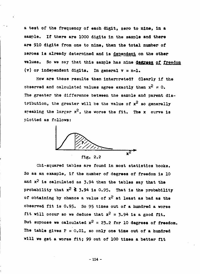
a test of the frequency of each digit, zero to nSne, in a

sample. If there are I000 di61ta in the sample and there

are 910 digits from one to nine, then the total number of

zeroes is already determined and is d__pende_on the other

values. So we say that this sample has nine _ o__f freedom

(v) or independent digits. In general v = n-1.

How are these results then interpreted? Clearly if the

observed and calculated values agree exactly then x2 = O.

The greater the difference between the samnle and parent dis-

tribution, the greater will be the value of x 2 so generally

sneaking the larger x2, the worse the fit. The x curve Is

plotted as follows:

fig. 2.2

Chi-aquared tables are found in most statistics books.

So as an example, if the number of degrees of freedom ms io

and x2 is calculated as 3.94 then the tables say that the

probability that x 2 _ 3.94 Is 0.95. That is the probability

of obtainin_ by chance a value of x 2 at least as bad as the

observed fit is 0.95. So 95 times out of a hundred a worse

fit will occur so we deduce that x2 = 3.94 ms a good fit.

But supoose we calculated x2 = 23.2 for lO de6rees of freedom.

The table gives P = 0.01, so only one time out of a hundred

will we get a worse fit; 99 out of lO0 times a better fit

- 114 -

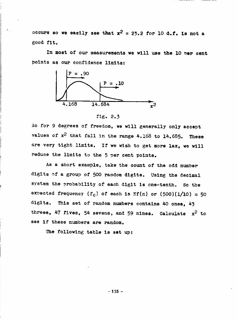
occurs so we easily see that x 2 = 23.2 for I0 d.f. Is not a

8ood fit.

In most of our measurements we will use the I0 _er cent

points as our confidence limits:

I

4.168 14.684 x2

fig. 2.3

So for 9 degrees of freedom, we will generally only accept

values of x2 that fall in the range 4.168 to 14.685. These

are very tight limits. If we wish to get more lax, we will

reduce the limits to the 5 per cent points.

As a short example, take the count of the odd number

digits of a group of 500 random digits. Using the declmal

system the probability of each digit is one-tenth. So the

eroected frequency (fc) of each is Nf(n) or (500)(1/10) = 50

digits. This set of random numbers contains 40 ones, 43

threes, 47 fives, 54 sevens, and 59 nines. Calculate x2 to

see if these numbers are random.

The following table is set up:

- 115 -

Table 2

n fo fc fo " fc (fo " fc)2

1 5O 4O i0 i00

3 50 43 7 49

5 5O 47 3 9

7 50 54 - 4 16

9 50 59 --9 81

255

x2 = _ (fo - %)2 = __255 -- 5.1

fo 50

x = 5.1 for 4 d.f. P _0.27

from equation 2.1

This is within the I0 per cent confidence limits so thls is

a _ood set of random numbers.

_TA:[DARD DEVIATION

The standard deviation wlll be used in conjunction with

the mean or average to gain certain knowledge about the random

digits.

It is defined as follows:

where: 0-= standard deviation

n = number of trials, etc.

In 6eneral the probability for a measurement to occur

in an interval within T_ of the median Is

e d.f. = desrees of freedom

- 116 -

PCT 24_J

-T

The _robabillty (see fig. 2.4)

is"

?(l) = 0.683

_(2) = 0.954

for a few values of T

l-P(l) : o.317

l-P(2) : 0.046

"(3) = 0._97 | 1-PC3) : 0.003

fis. 2.4

This means that the probability for a measurement to fall

within one standard deviation of the mean is about 68 per

cent, the probability of beln_ farther away than 2_ is _.6

per cent and farther away than 3_ is 0.3 per cent. So nor-

mally we should exDect about 30 per cent of the data to fall

outside the first standard deviation.

As an example, let us asaln take the odd numbered di61ts.

term inThe last column of Table lI is also the (re - fc) 2

the formula for standard deviation (equation 2.2). So then.

_" = 7.14

- 117 -

This gives the following results:

<r

2_

3_

Range

_2.86 to 57.1@

35.72 to 64.28

28.58 to 71.42

These results are very favorable.

# Readings Within Range

3

5

5

Three-flfths or 6Oper

cent fall within one _ compared with 68 per cent theoretically,

and none fall further than 2_away.

FREQUENCY TEST

This test is basically the comparison of the frequency

of occurrence of each digit O to 9 with the expected value

of the digit, i.e. one-tenth the number of digits in the

group. Chi-squared test and standard deviation are used to

see how close the digits are to the exoected.

Remember where this expected or parent distribution

comes from. We have mentioned that one of the properties of

random numbers is that each digit is equally probable and

even though we are generating pseudo-random numbers, this

property still holds true. So we are Justified in saying that

the expected value for the frequency of occurrence of a digit

is i/I0 the number of digits in a decimal system.

Variations of the frequency test would be running tests

on every other digit, every third digit,......., every tenth

digit, and also the frequency of odd digits to even digits

is often comoared as well as frequency of numbers below the

- 118 -

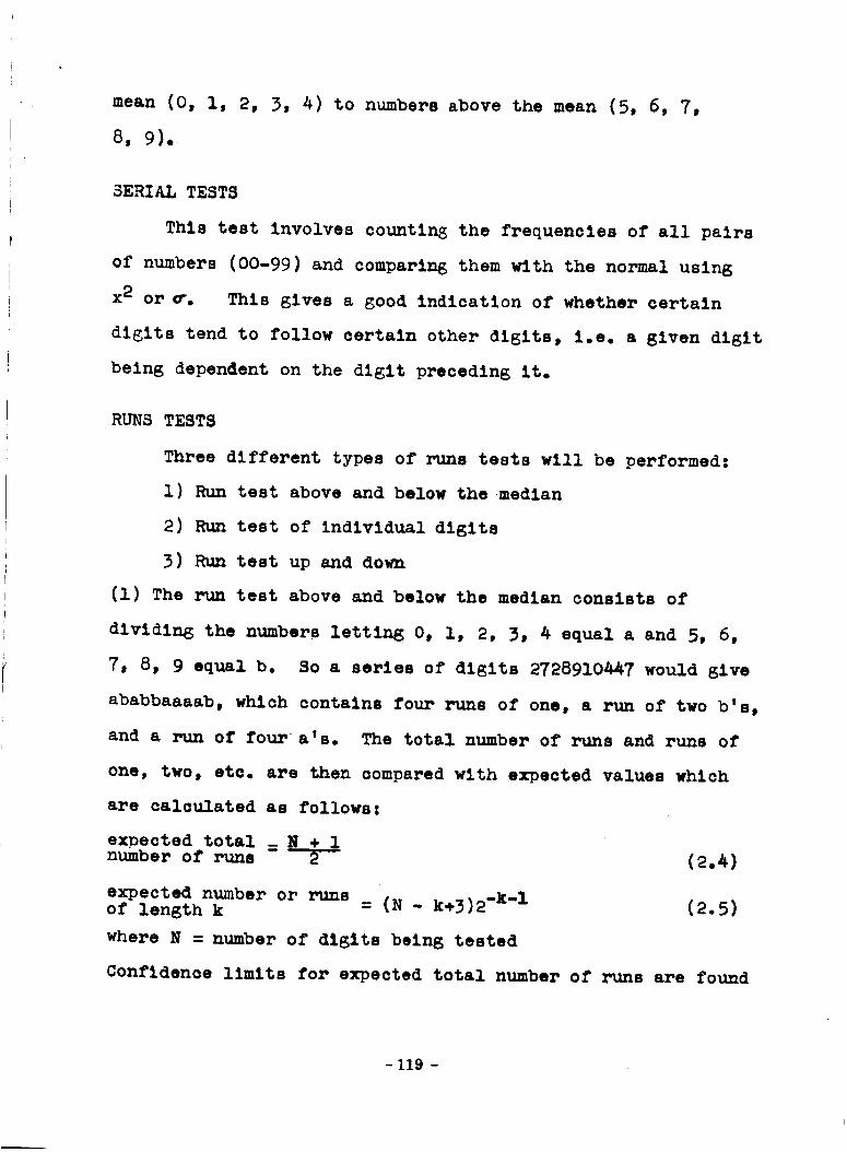
mean (0, I, 2, 3, 4) to numbers above the mean (5, 6, 7,

8, 9).

SERIAL TESTS

This test involves counting the frequencies of all pairs

of numbers (00-99) and comparlm6 them with the normal using

x2 or _. This gives a good indication of whether certain

digits tend to follow certain other digits, i.e. a given digit

being dependent on the digit preceding it.

RUNS TESTS

Three different types of runs tests will be performed:

i) Run test above and below themedian

2) Run test of individual digits

3) Run test up and down

(1) The run test above and below the median consists of

dividing the numbers lettin6 0, i, 2, 3, 4 equal a and 5, 6,

7, 8, 9 equal b. So a series of digits 2728910447 would give

ababbaaaab, which contains four runs of one, a run of two b's,

and a run of four a's. The total number of runs and runs of

one, two, etc. are then compared with ex_oected values which

are calculated as follows:

expected total _ N ÷ 1number of runs --"_ (2.4)

expected number or runsof length k = (N - k÷3)2 -k'l (2.5)

where N = number of digits being tested

Confidence limits for expected total number of runs are found

- 119 -

from abXe 47, else 20: [9].

A small mulls of this table fo:L_owss

Table 3

90 per cent l_itj

lowe_ limits u_pe_ linersn_beF of l_dnsexceeded (a)

200

200

300

4OO

50O

N.Bo

88 114

178 224

268 334

358 4_

448 554

For m>10, the numbe_ of r,ms is approxinately

normally distributed with mean m,l and variance (u 2) equal

to m(m-l)/(lm-l).

(2) The man test up and down conslmts in detezsalnln$ if the

differ,ences between successive dlslts Im positive or± nesatlve.

So for, N _olnts (uI, ul,......, u_) we write a blnar,y sequence

whose nth term Is "u" if _<Un+ l and is "d" If UnSUn+l.

So asaln for the sequence 2728910447 we set uduuddu-u, Lettlns

the dash be a "U" this contains two runs of one, two runs of

two, and one z_Au of three. The _osults are, of sou:so, then

compared by x 2 with expected values that ar_ calculated am

follows |

expected total = (IN-I)number' of runs 3

expected number, of mms _Sg+lof lensth i

(2.6)

[2.7)

- 120 -

expected number of runs

of length 2 = (2.8)

expected number of runs = 2k"+K+.LI_-_._+3_ -K'4 (2.9)of length k

where N = number of digits being tested.

As noted in the example above, often a dash will occur

in the case where Un = un+l. A 6cod way to overcome this

is to take the u's and d's from the start of the sequence

and use them in the place of each dash that turnm up.

- 121 -

CHAPTER III

ANALYSIS OF PROGRAMS

GE,._'RATED ON THE COMPUTER

INTRODUCTION

The background of random numbers noted and the tests

to be used understood, the discussion of the random numbers

that I have 6enerated on the computer can begin.

These programs will begin at the simplest level and

proceed toward the complex, but useful, methods. Each method

will generally be an improvement over the one precedlng It,

and these improvements will be emphasized a good Seal.

Consideration will also be given to variation of inputs and

the effects on the results. Chanter I discussed these methods

mutely from the mathematical viewpoint, the theoretical

side, but this chapter considers the problems of gettlng the

programs to work on a computer. _o cosrputer techniques will

be emphasized but will be tied in closely with the discus-

sions of Chapter I.

As an aid to understanding this chapter, the actual

Fortran lan6uage computer programs can be found Sn Apnendix

A while most of the actual numbers generated will be found

in Appendix B.

- 122 -

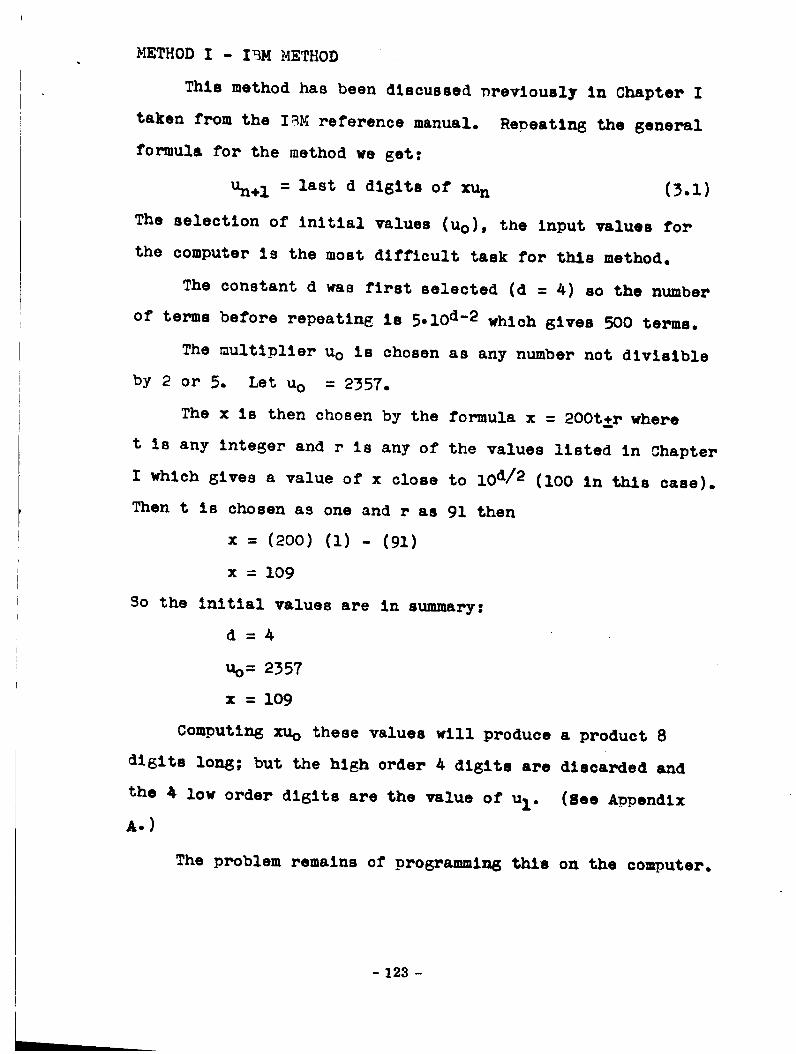
_THOD I - IBM METHOD

This method has been discussed nrevlously in Chapter I

taken from the I_M reference manual.

formula for the method we get:

Un+ 1 = last d digits of xu n

ReDeatin6 the general

(3.1)

The selection of initial values (Us) , the input values for

the computer is the most difficult task for this method.

The constant d was first selected (d = 4) as the number

of terms before repeating is 5.10 d-2 which gives 500 terms.

The multiplier u o is chosen as any number not divisible

by 2 or 5. Let uo = 2357.

The x Is then chosen by the formula x = 200t+r where

t is any integer and r is any of the values listed in Chapter

I which gives a value of x close to lod/2 (I00 in this case).

Then t is chosen as one and r as 91 then

x = (200) (1) - (91)

x = 109

SO the initial values are in summary:

d = A

us= 2357

x = 109

Computin 6 xu o these values will produce a product 8

dIsits lon6| but the high order A digits are discarded and

the A low order di61ts are the value of u 1. (See ADpendlx

A.)

The problem remains of pro_rammi_ thll on the computer.

- 123 -

The program was written entirely in fixed-point mode. To

show the effect of fixed point, suppose a certain product

is 767215.72. O_eratlon in this mode will discard the under-

lined digits leaving only +7215. So fixed-point mode rejects

all decimals and digits to the left of the four low order

digits. When the 8 digit product xu o is calculated, only

the four low order digits are _rinted. This is exactly the

u 1 that is required. This program consisted of numbers of

four digits in length and contained 500 terms before re-

peatln6 (see Appendix B). But looking at columns of numbers,

it is noticed that the period of each column is not 500.

The period for each column is

units column

tens column

hundreds column

thousands column

T=2

T =i0

T =50

T = 500

So the low order digits of the numbers are far from random.

The periodicity of the digits increases as the order of the

digit position increases.

The units column consists simply of the alternating

digits 3 and 7. This column can be discarded as not random.

The tens column is composed of the I0 digit series

1157933975. Each digit appears twice, but they are only odd

numbered digits. No even digits occur in this column so it

certainly is not random.

The hundreds column contains 50 digits before repeating.

- 124 -

Twenty are even and thirty are odd. The orobablltty is only

16 per cent that there could be 10 more odd digits than

even digits at these values,

(x 2 = _2+52 = 2 P = 0.16 for I d.f.)25

so the hundreds column Is rejected.

The thousands column consists of 500 digits distributed

as follows:

51 zeroes

50 ones

50 twos

50 threes

50 fours

49 fives

Calculating x2 61yes:

50 sixes

50 sevens

50 eights

50 nines

x2 = i + 8(0) ÷ 1 = 0.04 for IO degrees of freedom.5o

From the x 2 table a x2= 0.04 gives a probability P =

0.999999.... for 9 d.f. This means that only one chance

in iO,O00...., will give a better fit. So it seems logical

that this is a good set of random numbers. But statisticians

caution about numbers that are too close to the norm. When

numbers get too close to what is expected, they cease to be

random. Hence we have mentioned before that limits of x 2

for acceptable results are the ran6e 4,168 to 14.684. This

lower limit is chosen to avoid these numbers that follow

the norm too closely and are as a result not random. For

this reason the numbers in the thousands column must be

rejected.

- 125 -

The entire method I is rejected then for the various

reasons cited.

I/_ETHOD II - IS_ROVED IBM METHOD

It was the our_ose of this method to attempt to make

improvements on Method I so that every column in Method II

would be random instead of just one column.

In Method I it was the last digit which was least random

so in this method the last digit is eliminated. After the

oroduct xu o has been com_uted and the first four di6its are

drop oed, the remaining digits (formerly u I) are now divided

b;T the constant I0. So if u I was equal to 4A87, dividing

b:_ i0 6ives 448.7. But in the computer lanEuaEe (Fortran

language) this number is in flxed-polnt mode so only the

digits 448 are retained as the new u 1.

Two statements are taken from Appendix A to show the

difference in com_uter language

7 I(J) = N*K ..... .......Method I

7 I(J) = N*K/N .... ......Method IX

where

7 = statement number

I(J) = u(n.l)

N=X

K =u n

Let us now see if this improvement has helped _enerate

numbers that are more random. Ninety-seven numbers of three

- 126 -

digits each were generated before they started reoeatin_.

(See Aprendix B.) Already an improvement can be seen. The

hundreds column of Method I had a period of 50 while in this

pro6ram this column has a period of 97. The other columns

also have the same period, and hence it is increased many

times over Method I.

a) Frequency Tests: There are 291 di6its so there should

be statistically speakln_ 29.1 of each digit. The frequency

test on these digits gave the following table which is

similar to table 2 in Chapter II:

Table 4

n fc fo fo - fc (fo - fc )2

0 29.1 29 0.I 0.01

i 29.1 27 2.1 4.40

2 29.1 31 1.9 3.60

3 29.1 23 6.1 37.30

4 29.1 29 0.I 0.01

5 29.1 32 2.9 8.40

6 29.1 3A A.9 2A.O0

7 29.1 27 2.1 4.40

8 29.1 30 0.9 0.81

9 291 29 0.I 0.01

291.0 291 82.94

x 2 = 82.94 = 2.84 for 9 d.f.29.1

P = .965

- 127 -

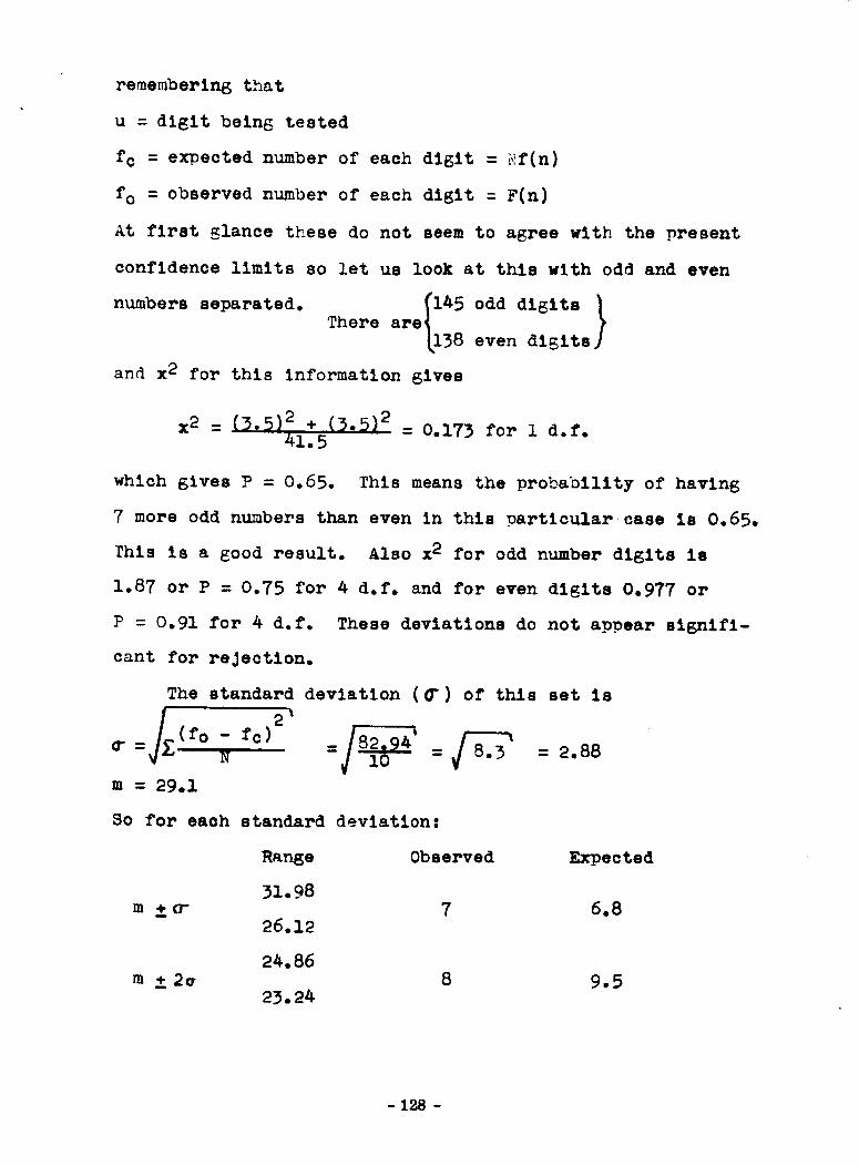
rememberln6 that

u = dight beins tested

fc = expected number of each digit = _f(n)

fo = observed number of each digit = F(n)

At first glance these do not seem to agree with the present

confidence limits so let us look at this with odd and even

numbers separated. There I_I145°dd diglts }arek_38 even digits

and x 2 for this information gives

x2 = (3"5)2 ÷ (3"5)2 = 0.173 for I d.f.41.5

which gives P = 0.65. This means the probability of having

7 more odd numbers than even in this oarticular case is 0.65.

This is a good result. Also x2 for odd number digits is

1.87 or P = 0.75 for 4 d.f. and for even digits 0.977 or

P = 0.91 for 4 d.f. These deviations do not appear signifi-

cant for rejection.

The standard deviation (_) of this set is

= N _ I0 =

m = 29.1

So for each standard deviation:

Range Observed

31.98

m _o- 726.12

24.86

= 2.88

Expected

6.8

m _2e 8 9.523.24

- 128 -

m_3o-

Range Observed Exoec ted

37.74

lO 9.92o.36

There are only two readings Dast 3_. All the others fall

within range.

b) Runs Tests: A run test above and below the mean was

performed with the followin6 results:

number of runs counted .................. 155

number of runs expected ................. 146

rar4_e nermitted as 90rer cent limits ......................... 134 - 160

These results were good.

A run test uD and down was also Derformed. There

were 194 runs exoected and 206 observed. For 90 per cent

limits the range allowed is from 173 to 217. The observed

value falls within this limit.

According to these tests there is little evidence

of any divergence from the normal exTectations. Only in

the frequency test of these numbers is the result ques-

tionable. So we can conclude that these numbers are random,

but there is one glaring fault with these random numbers.

There is not enough of them. There are only 97 terms in

the series; far from enough to apply this method to a Monte

Carlo method.

- 129 -

_ETHOD III- CENTER SQUARING METHOD

So far the methods that have been investigated have

consisted of multiplying various numbers with a definite

constant over and over. A better way for generation would

be to have two new multipliers for each number generated.

This method (Yon _eumann's Center Squarln6 Method)

has been discussed in 6teat detail in Chapter I. Short

cycles have been obtained by some people that have used this

method.

Three sets of random numbers were senerated on an adding

machine usln_ three different initial values of ao_

a o = iiii 6ave 54 terms

a 0 = 1234 " 82 "

a O = 6043 " 66 "

These give an averase period of 67 numbers of four digite

each. (See Appendix B).

For a o = 1234 (82 terms) the frequency test _ives:

0-9 3-10 6-6

1-13 4-9 7-5

2-13 5-8 8-8

9-3

This has x 2 = 11.75 for 9 d.f. or a P = 0.23 which is

good. But notice the digits divided in this manner:

(i, 2, 3, 4, 5) = 53 digits_

i(6, 7, 8, 9, o) = 31 "av. = 42

- 130 -

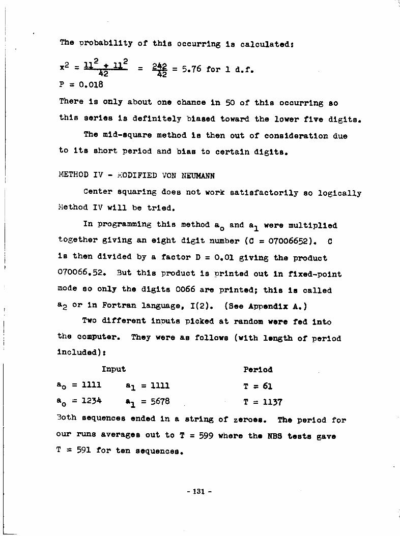
The orobabillty of this occurring is calculated:

=P = 0.018

There is only about one chance in 50 of this occurrln6 so

this series is definitely biased toward the lower five dislts.

The mid-square method is then out of consideration due

to its short period and bias to certain digits.

METHOD IV - _ODIFIED VON NEUMANN

Center squaring does not work satisfactorily so loglcally

Method IV will be tried.

In programming this method a o and a I were multiplied

tosether giving an eight digit number (C = 07006652). C

is then divided by a factor D = 0.01 giving the product

070066.52. But this product is printed out in flxed-polnt

mode so only the digits 0066 are printed; this is called

a2 or in Fortran lar_uage, I(2). (See Ap_endlx A.)

Two different inputs picked at random were fed into

They were as follows (with length of periodthe computer.

included):

Input

a O = Iiii aI = iiii

a o = 123A a I = 5678

Period

T = 61

T = 1137

Both sequences ended in a strin_ of zeroes. The period for

our runs averages out to T : 599 where the NB8 tests gave

T = 591 for ten sequences.

- 131 -

It was virtually impossible to run any tests on the

_rogram resulting from the first inDut. However, some

indication is given that thls might be a good method by

looking at the frequencies of the digits:

16 zeroes 23 threes 18 Sixes

20 ones 21 fours 14 sevens

16 twos 17 fives 16 eights

18 nines

Thls gives an x2 = 3.72 for 9 d.f. or ? = 0.92. So nine

times out of ten a worse fit will occur.

The frequency of digits for the second input were as

follows:

212 zeroes

216 ones

203 twos

174 threes

192 fours

205 fives

213 sixes

191 sevens

206 eights

188 nlnes

These were from a test of the first 250 numbers of four

digits each. So for two thousand digits we eroect two hun-

dred of each number. Table 5 contains the frequency test.

These two tests show very good results concerning the

randomness of these numbers. The probabilities for the fre-

quency and odd versus even test were well within the confidence

limits which we set. _See Table 5,)

- 132 -

Table 5

n fc fo

0 200 212

i 200 216

2 200 203

3 200 174

4 200 192

5 2O0 205

6 200 213

7 200 191

8 200 206

9 200 188

x2 = 1604 = 8.022OO

P = 0.52 for 9 d.f.

For odd versus even we get

n fo fc

odd 974 i000

even 1026 i000

x 2 = 1352 = 1.352 for I d.f.I000

P --=0.25

fo " fc (fo - fc )2

12 144

16 256

3 9

-26 676

- 8 64

5 25

13 169

- 9 81

6 36

12

1604

fo - fc (fo - fc) 2

-26 676

+26 676

A runs test above and below the median was taken with

the followln_ results :

- 133 -

Table 6

Length of Run Observed Expected

1 479 5OO. 5

2 268 250.1

3 135 125.0

4 59 62.4

5 31 31.3

6 13 15.7

7 i0 7.8

8 4 3.9

9 __11 2,o

Total iOOO 998.7

The results of thls runs test are very good; and along

with the frequency test, these 5ire very good indication

that the numbers generated in this method are random.

_THOD V - LEHMER'S METHOD

This Is the method devised by D. H. Lehmer as was dis-

cussed In Chapter I, Section D.

Lehmer's formula is summarized:

Un = 8_Do _23Un-i- 2_DO (23_-i)_ (3.2)

where RHDO = right hand disits of

LHDO = left hand digits of

In terms of congruences this is written (accoPdin 6 to Lehmer)

as

Un = Uo23n(mod 108 + i) (3.3)

- 134 -

which gives 5,882, 352 eight digit numbers.

The IBM 1620 was better adapted to _roduce a six digit

number as m result. So the initial value Un Is an el@ht

dlglt number, but this formula is used:

= 6 Do [23u _1 - 23 _l)] (3.4)as opposed to equation (3.3)

In the actual generation of the numbers(see Appendix

A and B) certain problems arose with exponents exceeding

the computers E_99 limit. So three IF statements were used

in the program to limit these exronents. This particular

program prints out 801 six digit numbers; 4806 random digits

total for each input apolied. The program can be continued

by using its last number as the input to the continued

program.

Testing will now begin to determine whether these

numbers are acceptable for use.

FREQUENCY TESTS

With 4806 random digits we expect 480.6 of each digit.

results of countin_ were:

470 threes

505 fours

450 fives

511 zeroes

490 ones

475 twos

To calculate x 2, a

459 sixes

473 sevens

483 ei@hts

490 nines

chi-squared table is set up.

The

- 135 -

Table 7

n fo £c (fo " fc) (fo - fc)2

0 511 480.6 30.4 924.16

1 490 480.6 9 •4 88.36

2 475 480.6 - 5.6 31.36

3 470 z_80.6 - 10.6 112.36

4 505 480.6 24.4 595.36

5 450 480.6 - 30.6 936.36

6 459 480.6 - 21.6 466.56

7 473 480.6 - 7 •6 57.76

8 483 480.6 2.4 5.76

9 490 480.6 9.4 88.36

33o6.40

x2 = Z (fo - fc) 2fc

= 3306.4 = 6.879 for 9 d.f.a80.6

This 5ives P = 0.65

For odd digits

x 2 = _ = 2.67 for 4 d.f. (P = 0.60)

For evem digits

x2 = _ = 4.20 for 4 d.f. (P = 0.38)

So the x2 value for 9 degrees of freedom is 6.879 and the

probability of exceeding this value is approximately 0.65.

The total number of even digits is 2433 as against 2373

odd digits. Assumln6 that an even digit is as likely to

- 136 -

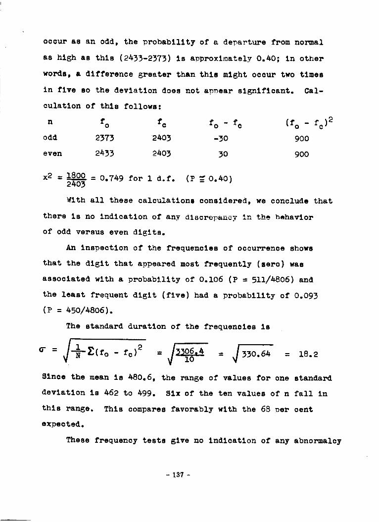
occur as an odd, the Drobabillty of a derarture from normal

as high as thls (2433-2373) Is aoproxlmately 0.40; In other

words, a difference greater than thls might occur two times

in five so the deviation does not apoear significant. Cal-

culatlon of thls follows:

n fo fc fo - fc (fo - fc )2

odd 2373 2403 -30 900

even 2433 2403 30 900

x2 = 1800 _ 0.749 for I d.f. (P _ 0.40)2403

With all these calculations considered, we conclude that

there Is no indication of any discrepancy in the bohavlor

of odd versus even digits.

An inspection of the frequencies of occurrence shows

that the digit that appeared most frequently (zero) was

associated with a probability of 0.106 (P = 511/4806) and

the least frequent digit (five) had a probability of 0.093

(P = 450/4806).

The standard duration of the frequencies is

o-= J ° _ fc)2 = #33o.64 = 18.2

Since the mean is 480.6, the range of values for one standard

deviation is 462 to 499. Six of the ten values of n fall in

this range. This compares favorably with the 68 per cent

expected.

These frequency tests glve no indication of any abnormalcy

- 137 -

compared with normal distribution.

SERIAL TEST

The frequency of the occurrence of all noesible pairs

of dl_its is 61yen in Table 8. It was formed by entering

the pair of digits iJ Into the ith row and the Jth column.

Table 8

Serial Test

Frequency of Ist Digit

Frequency of 2nd Digit

2 5 _ 5

0 52

1 55

2 56

3 51

4 5O

5 51

6 43

7 46

8 63

9 44

I U*O I 6 7 8 9 TotalI

51 55 51 47 51 51 47 511

47 60 52 44 52 39 48 39 54 490

49 37 43 53 37 51 51 60 37 474

51 41 41 60 41 41 44 41 58 469

54 44 56 41 55 41 54 53 51 505

49 44 47 46 38 38 43 52 41 448

49 46 47 44 46 54 47 40 45 458

54 53 55 49 41 43 47 36 48 472

41 46 45 49 49 48 50 46 46 483

45 48 32 55 48 51 57 65 63 490

4800Tot 511 490 474 469 505 _8 458 472 483 490

Only 4800 of the 4806 digits were used in this test; the

last 6 waits were ignored.

Thls test is performed %o show that the table is a

random sample from a sequence in which one _air of disits

- 138 -

is as likely to occur as another.

The chl-squared test compares the frequency (fo) in

each position of the table with the expected frequency

(fc = 48). The number of degrees of freedom, v, is 90 due

to the constraint that totals of corresponding rows and

columns are the same.

We find:

x2 = 4161 = 86.69 for 90 d.f.48

P= 0.40

This is within our confidence limits so by the serial test

thls sequence of numbers seems to be random.

RUNS TESTS

This will be the most severe test performed on the

numbers. Havin_ passed the frequency and serial tests, these

digits will certainly be random if they can get by the runs

tests. A set of non-pseudo random numbers may get past one

or two tests but will certainly not get past all three tests.

Three runs tests were performed: runs test above and

below the median, runs test up and down, and runs test of

individual numbers as are explained in Chapter If.

(1) Above and below the median:- All the generated numbers

were used in this test and 5, 6, 7, 8, and 9 were considered

above the median while O, I, 2, 3, and 4 were below the

median. Table 9 shows the results of this test.

- 139 -

Table 9

Length of Runs Expected Observed % Error

1 1202.00 1143 - 4.9%

2 600.90 600 - .1%

3 300.40 267 - II. 1%

4 150.20 158 + 5.2%

5 75.06 72 - 4.1%

6 37.50 32 - 14.7%

7 18.76 19 + 1.3%

8 9.39 7 - 25.5%

9 4.68 6 + 28.2%

io 2.34 5 + 28.6%

ll 1.17 2 + 71.0%

12 O. 59 .._ +230.0%

2401.82 2311 - 3.8%

Range for the Total (90% limits) : 2258-2534

The exoected values were calculated using the formulas

given In Chapter IX. Per cent error was calculated for

each length of run. For 4806 digits, 2402 runs are expected

but with a 90% leeway allow, the expected range is 2258 to

2534. The Lehmer method produced 2311 runs which is within

the 90 Der cent confidence limits.

The observed number of runs for the smaller lengths

(i to 6) fall below the expected amount on the average while

lensths seven to twelve fall above the expected amount. But

the excess of higher order runs does not effect the total

- 140 -

Dicture too much since there are only thirteen runs from

lengths nine to twelve anyway. The difference between ob-

served and exnected runs of lengths one and three (59 and

33 digits resnectively or 92 digits as compared with the 91

digit differential of the total) actually cause the deficiency,

for the most Dart, in the total number of runs observed with

respect to the number exnected; but as was shown, this total

is well within the 90% limits. This test then gives no indi-

cation of these numbers not being pseudo-random.

(2) Up and down:- This test was performed on 914 of the 4806

digits. Again exoected values were calculated for Chapter

II expressions, and the results given in Table i0.

Table I0

Length of Rune Expected Observed

1 382.40 365

2 168.10 158

3 48.20 45

4 i0.50 13

5 1,87

Totals 611.07 585

Note that 611 runs are expected and 583 are observed.

The observed total is 4.6% in error of the =alculated

value which is a rather good result. The counts for indi-

vidual lengths of runs also give no indication of the level

of these numbers varying too slowly or too quickly.

(3) Individual numbers:- This test was performed on all

- 141 -

the numbers. The exnected values were estimated from a

test of similar nature by the Rand Cor_oratlon [ll]. The

results follow: Table II

LenEth of Run E_ected _served

1 3898.0 3958

2 389.8 369

3 38.9 39

4 3.9 3

5 0.4 O

Totals 4331.O 4369

The total number of runs counted are off from the

exnected value by only 0.884. This is an excellent result

and more or less confirms the decision that these numbers

are pseudo-random.

CONCLUSION.

Ample evidence for the pseudo-randomness has thus been

given. The first Oroperty of total unwredictability has

been upheld by the serial test and runs testa. The serial

test showed that no two digits depended on each other overall

while the runs tests Oroved that the digits were not dependent

on their preceding or following digit. They were, in fact,

unpredictable. Secondly, it was shown that the digits were

equally orobable by the results of the frequency test on the

ten different digits involved.

We thus conclude that none of these tests contradict

- 142 -

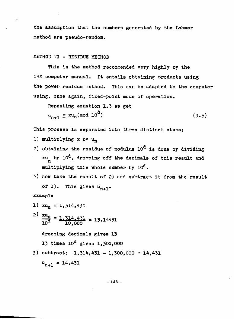
the assumption that the numbers generated by the Lehmer

method are pseudo-random.

)_THOD VI - RESIDUE I_ETHOD

This is the method recommended very highly by the

IBM computer manual. It entails obtaining products usln_

the power residue method. This can be adapted to the computer

using, once again, fixed-polnt mode of operation.

Repeating equation 1.3 we get

Un+ 1 - xu n(mod i0 d) (3.5)

This process is separated into th__ee distinct steps:

I) multiDlying x by un

2) obtaining the residue of modulus I0 d is done by dividing

xu by lO d, droDping off the decimals of this result andn

multiplying this whole number by lO d.

3) now take the result of 2) and subtract it from the result

of 1). This gives Un+ 1.

Example

l) xu n = 1,314,431

2) xu n _ 1.314.431 = 13.14431- iO, 000

dronDing decimals gives 13

13 times I0 d gives 1,300,000

3) subtract: 1,314,431 - 1,300,000 = 14,431

Un+ I = 14,431

- 143 -

Let us now put these series of events into a simple equation

which requires only the basic arithmetic operations (addition,

subtraction, multiplication, and division).

_÷I :_- XUnI0_ lod(3.6)

2

where operation 2 is that sneclal division which ignores

remainders (drops off decimals).

This equation can now be anplied very nicely to the

computer as follows:

i) let Y = X-U(N) (same as operation i in equation 3.6)

2) let J = Y/P where P = IO d and J is _ fiA_d pc 4_+

variable. Fixed point is ideal for operation 2 because

it drops off decimals and retains only whole numbers.

3) let Z = J thus puttln_ this whole number into floati_-

point mode so it matches up with other variables in the

(3.7)

equation.

_) the final computer equation is

U(N+I) = Y-Z*P

(See A_endix A.)

Equation 1.3, 3.6, and 3.7 then are all the same, but the

last two grew from the need of the simple operations that

are required on the computer.

The numbers generated by this method (see Apoendix B)

were tested for randomness by the usual statistical tests.

The list consisted of five diEit numbers with only _eroes

- 144 -

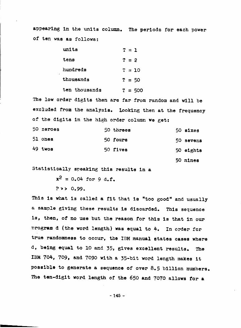
appearing in the units column.

of ten was as follows:

units

tens

hundreds

thousands

ten thousands

The periods for each power

T=I

T=2

T =i0

T =50

T = 500

The low order digits then are far from random and will be

excluded from the analysis. Looking then at the frequency

of the digits in the high order column we get:

50 zeroes

51 ones

49 twos

50 threes

50 fours

50 fives

50 sixes

50 sevens

50 eights

50 nines

Statistically speaking this results in a

x2 = 0.04 for 9 d.f.

P'> 0.99.

This is what is called a fit that is "too good" and usually

a sample giving these results Is discarded. This sequence

is, then, of no use but the reason for this is that in our

Drogram d (the word length) was equal to 4. In order for

true randomness to occur, the IBM manual states cases where

d, being equal to IO and 35, gives excellent results. The

IBM 704, 709, and 7090 with a 35-bit word length makes it

possible to generate a sequence of over 8.5 billion numbers.

The ten-dlglt word length of the 650 and 7070 allows for a

- 145 -

sequence of 500 million terms.

So using these other com_uters, this becomes probably

the best method available today for generating random numbers.

But the numbers nroduced by the 1620 must be discarded.

CONCLUSION

As a result of these tests then, it is rather apparent

that this sample distribution of numbers generated by the

residue method is inadequate. The most evident failing Is

that the length of the period of these numbers ms too short

(T = 500) for use In any large scale Monte Carlo nroblems.

The reason for this Is that the IBM 1620 limits us to a five

digit output using fixed-polnt arithmetic on thls computer.

This can be overcome on the other computers recommended that

have a longer word length. Uslr_E a d = 8 or higher on another

machine will give a much longer cycle.........T = 5-I0 d-2

so the period will be flve million terms or higher; surely

enough for anyone's desires.

Taking these things into consideration along with the

results of all six methods and the type of com_uter that was

available, it has been decided that method five (D. H. Lehmer'a

method that was modified to fit the IBM 1620) is the one

which best flts the properties of a pseudo-random number.

Observe the following: The Improved IBM method passed all

the statistical tests (but so dld the Lehmer method), the

Modified Von Neumann method had a long cycle (but so dld

- 146 -

the Lehmer method) and Lehmer's is a quick source of

numbers obtainable directly from a computer.

From this statement, it is clear that only the Lehmer

method is i) truely pseudo-random, 2) is of Ion6 cycle, and

3) is easily obtainable from the computer that was made

available to us.

This method then will be used in Chapter IV in the

Monte Carlo application. Good apnroxlmations from the Monte

Carlo _roblem will be further evidence that the Lehmer method

is a good source for pseudo-random numbers.

This next method is considered merely from a curiosity

point of view to see Just how 6ood or bad the numbers from

a roulette wheel really are with respect to randomness.

METHOD VII - ROULETTE METHOD

Leaving now the arithmetic processes behind, we turn

to a physical process which is manually controlled; that

is, the spinning of a roulette wheel. Thou6h this process

cannot be seriously considered as a prime source of random

di6its (the method is much too slow); nevertheless, it will

be Interestln6 to see how this physical process comDares

with the fast arithmetic processes for randomness.

A small roulette wheel was used for this experiment

and the followin8 procedure was usedl

- 147 -

IF THESE NUMB_S THESE DIGITS

CAME _ ON THE _ USED AS

ROULETTE WHEEL .......... _N_M NUMBE_

10 to 19 .......... used so 17 bec_e 7 and

ii to 29 30 became 0 etc.

30 to 36 _ _ these numbers were not used since they

foooeetoo

double ze_ would have _balanced the system

Usi_ this method 2,200 disits were oroduced. The results

of the tests follow.

FREQU_CY TEST:

The frequency test _roduced the following data:

Table 12

n fo fc fo - fc (fo - fc )2

0 205 220 -- 15 225

1 184 220 --36 1296

2 212 220 - 8 64

3 208 220 -- 12 144

4 225 220 5 25

5 194 220 --26 676

6 265 220 45 2025

7 187 220 - 33 1089

8 262 220 42 1764

9 2.58 220 38 14_.__

2200 2200 8752

x2 = _ = 39.8 for 9 d.f. (P_(<O.OI)22u

- 148 -

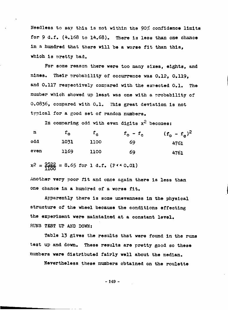
Needless to say thls is not within the 90% confidence limits

for 9 d.f. (4.168 to 14.68). There Is less than one chance

In a hundred that there will be a worse fit than this,

which Is nretty bad.

For some reason there were too many sixes, eig_hts, and

nines. Their probability of occurrence was 0.12, 0.119,

and 0.117 respectively comoared wlth the exoected 0.i. The

number which showed up least was one with a orobability of

0.0836, compared wlth 0.I. Thls great deviation is not

typical for a good set of random numbers.

In com_arln8 odd wlth even digits x 2 becomes:

n fo fc fo - fc (fo - fo )2

odd 1031 II00 69 4761

even 1169 Ii00 69 4761

x2 = 9522 = 8.65 for I d.f. (P,-O.OI)ii00

Another very poor fit and once again there is less than

one chance in a hundred of a worse fit.

Apparently there Is some unevenness In the physical

structure of the wheel because the conditions effectln_

the experiment were maintained at a constant level.

RUNS TEST UP AND DOWN:

Table 13 gives the results that were found in the runs

test up and down. These results are pretty good so these

numbers were distributed fairly well about the median.

Nevertheless these numbers obtained on the roulette

- 149 -

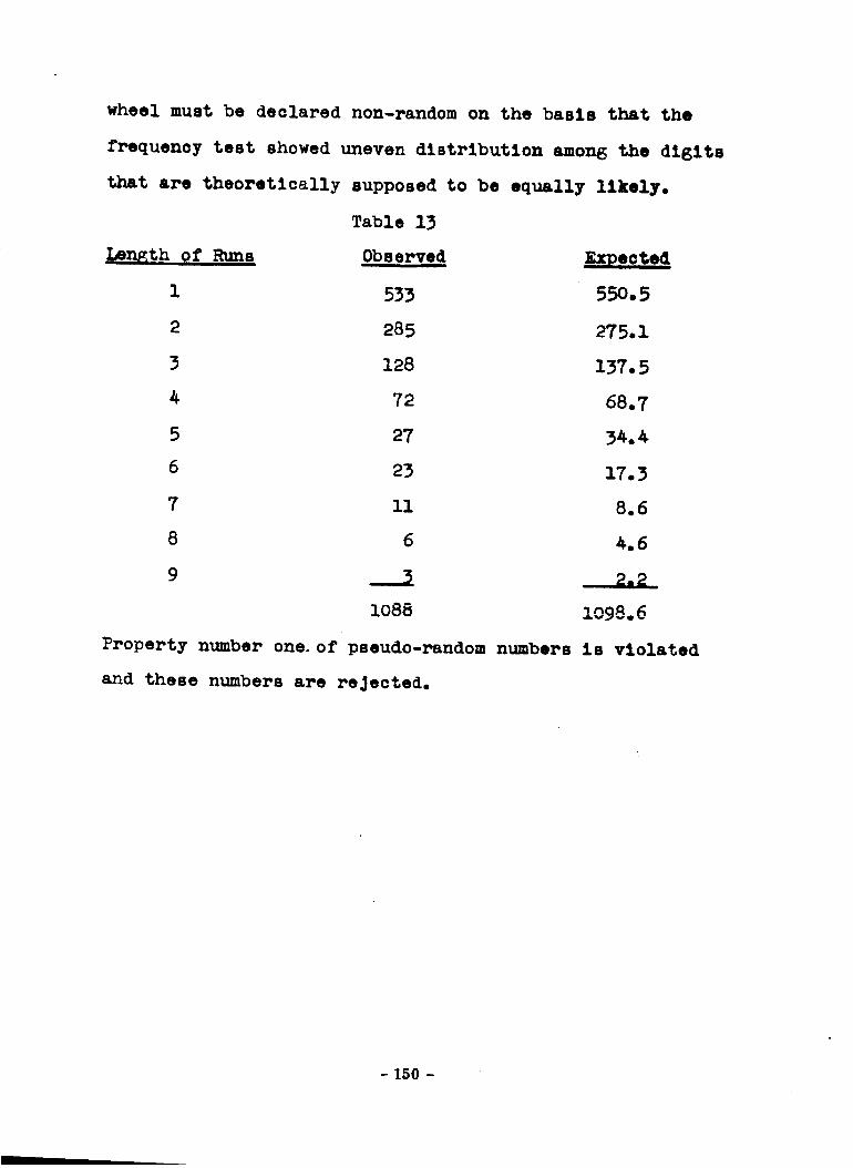
wheel must be declared non-random on the basis that the

frequency test showed uneven distribution amon_ the digits

that are theoretically supposed to be equally likely.

Table 13

Len_jth of Runs Observed Ex_ecte4

1 533 55o.5

2 zB5 275.1

3 128 137.5

4 72 68.7

5 27 34.A

6 23 17.3

7 II 8.6

8 6 4.6

9 ...._/ _.....L.L.

1088 _no_

Property number one. of pseudo-random numbers is violated

and these numbers are rejected.

- 150 -

APPENDIX A

FORTRAN LANGUAGE PROGRAMS

This is a comnlete list of the Fortran lan6ua6e programs

used to generate the random numbers in this paper.

METHOD I

Initial quantities: x = N = 109, uo = K = 2357

DIMENSIONI(I000)PRINT 2

_RINT 4

J--I

N--I09

READ I,K ....input card: 23577 I(_)_*K

TYPE ),I(J)

IF (J-lO00)5, 5, 6

J--_+l

GOT076 STOP

i FORMAT (I4)2 FORMAT (}6RHANDOM NU_ERS GENERATED BY IBM 1620//)

3 FORMAT (I6)

4 FORMAT (13HM=I09 K=2357//)END

METHOD II

Initial quantities:

DIMENSION I (I000)PRINT 2

PRINT 4

J=l

K=2357L=IO

x = N = 91, u O = K = 2357, L = 10

(program continued on next pa6e)

- 151 -

READ I,N

7 I(J)=.*K/N•...input card: 0091

TYPE 3,I(J)

J-lO00 )5,5,65 INFI IJ)

J--J+l

GOT076 STOP

1 FORMAT I14)2 FORMAT 36HRANDOM NUMBERS GENERATED BY IBM 1520//)

3 FORMAT II6)4 FORMAT 12HN--91 K=2357//)

END

METHOD III

The random numbers for this method were not generated on the

IBM computer; an addinsmachine was used•

METHOD IV

Initial quantities: i) aO = A = IIIi, a I = B = Iiii, D = 0.01

2) aO = A = 1234, a I = B = 5678 D = O•01

DIMENSION I (1300)

J=3PRINT 2

READ I,A,B,D7 C--A*B

I (J)=C*DF=I(J)

•... input card:

PUNCH 3, FIF (J-1300) 5, 5, 6

5 A=BB=F

J--J+l

GO TO 76 STOP

1 FORMAT 12F6.0,FIO.6!2 FORMAT 131-_=1nl B,nn,//)

3 _m_T (_.O)

iiii. IIii. 0.O11234, 5578• 0.01

152 -

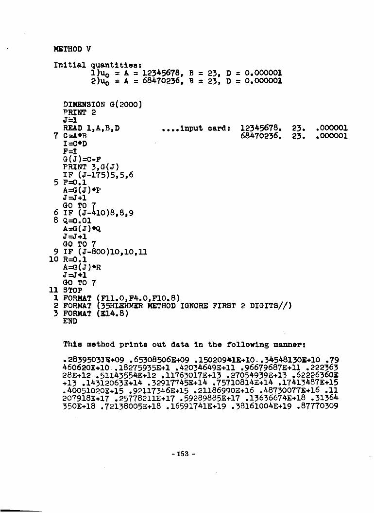
METHOD V

Initial quantltles.

l)u o = A = 12345678, B = 23, D = 0.000001

2)U O A = 68470236, B = 23, D = 0.000001

DIMENSION G(2000)_RINT 2

J=l

READ 1,A,B,D ....input card: 12345678.7 C=A*B 68470236.

I--CeDF=I

G(J)=C-FPRINT 3,G(J)

IF (J-175)5, 5,65 P=O.I

A=G(J)ePJ--J+l

GO TO 7

6 IF (J-410)8,8,98 Q=O. Ol

A=G(J)4,qJ--J+l

GO TO 7

9 IF (J-8OO)lO,iO,lliO R--O. i

A--G(J)eR

J--J_l

GO TO 7Ii STOP

I FORMAT (FII.O,F4.0,FIO.8)2 FORMAT (35HLEHMER METHOD IGNORE FIRST 2 DIGITS//)

3 FORMAT (EIA. 8 )END

23. •0OO00123. •00OO01

This method prints out data in the following manner:

.2839503]E+09 .65308506E+09 .15020941E+IO..34548130E+lO .79

460620E+I0.18275935E+I .42034649E+11 .96679687E+11 .222363

28E+12 .51143554E+12 .I1763017E+13 .27054939E+13 .62226360E

+13 .14312063E+14 .32917745E+14 .75710814E+14 .17413487E+15

.40051020E+15 .921173_6E+15 .21186990E+16 .48730077E+16 .ii

207918E+17 .25778211E+17 .59289885E+17 .13636674E+18 .31364

350E+18 .72138005E÷18 .16591741E+19 .38161004E+19 .877703O9

- 153 -

METHOD VI

Initial quantities: x = 3379, uo = u(o) = 389, P = 100000

DIMENSION U(2000)PRINT 2

N=O

READ I,X,U(N),P

7 Y--X*U(N)J=Y/P

....input card: 3379. 389.

Z--JU (N+I )=Y-Z*P

PUNCH 3,U(N+I)

IF (N-2000)5,5,65 N=N÷I

GO TO 76 STOP

1 FORMAT (FS.0,F6.0,FS.0)

2 FORMAT (33HRESIDUE METHOD IGNORE LAST 2 NOS.//)3 FORMAT (F9.0)

END

I00000.

154 -

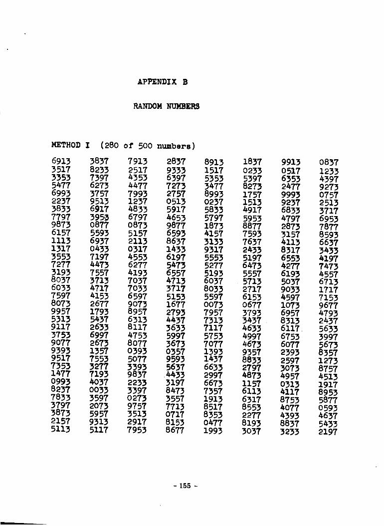
APPENDIX B

RANDOM NUMBERS

METHOD I (280 of 500 numbers)

6913 3837 7913 2837 8913 1837 9913 0837

3517 8233 2517 9333 1517 0233 0517 12333353 7397 4353 6397 5353 5397 6353 4397

5477 6273 4477 7273 3477 8273 2477 9273

6993 3757 7993 2757 8993 1757 9993 0757

2237 9513 1237 0513 0237 1513 9237 2513

3833 6917 4833 5917 5833 4917 6833 3717

7797 3959 6797 4653 5797 5953 4797 69539873 0877 0873 9877 1873 8877 2873 7877

6157 5593 5157 6593 4157 7593 3157 8593

1113 6937 2113 8637 3133 7637 4113 6637

1317 0433 0317 1433 9317 2433 8317 3433

3553 7197 4553 6197 5553 5197 6553 4197

7277 4473 6277 5473 5277 6473 4277 7473

3193 7557 4193 6557 5193 5557 6193 45578o37 3713 7037 4713 6037 5713 5037 6713

6033 4717 7033 3717 8033 2717 9033 1717

7597 4153 6597 5153 5597 6153 4597 7153

8073 2677 9073 1677 0073 o677 lO73 9677

9957 1793 8957 2793 7957 3793 6957 4793

5313 5437 6313 4437 7313 3437 8313 24379117 2633 8117 3633 7117 4633 6117. 5633

3753 6997 4753 5997 5753 4997 6753 3997

9077 2673 8077 3673 7077 4673 6077 5673

9393 1357 0393 0357 1393 9357 2393 8357

9517 7553 5077 9593 1437 8833 2597 1273

7353 3277 3393 5637 6633 2797 3073 8757

1477 7193 9837 .4433 2997 4873 4957 4513

0993 4037 2233 3197 6673 1157 0313 1917

8237 0033 3397 8473 7357 6113 4117 89537833 3597 0273 3557 1913 6317 8753 5877

3797 2073 9757 7713 8517 8553 4077 0593

3873 5957 3513 0717 8353 2277 4393 4637

2157 9313 2917 8153 0477 8193 8837 5433

5113 5117 7953 8677 1993 3037 3233 2197

- 155 -

METHOD Ill (All numbers included)

998 285 744 753 033 587 463 035 910 204

228 174 360 482 778 355 129 249 487 082

739 011 852 607 374 673 408 689 785 327

182 592 816 069 151 626 458 397 024 073897 534 331 263 590 548 950 572 656 206

422 863 016 989 063 163 915 820 619 554

465 409 771 107 849 419 665 274 898 577

600 401 724 219 109 758 740 581 658

420 515 646 618 691 660 418 941 090994 385 262 662 868 562 552 793 213

METHOD llI (three Inwuts)

I) ao = Iiii

iiii 0228 6756 9606 0342 7758 5980 4996

2343 0519 6435 2752 1169 1865 7604 9600

4896 2693 4092 5735 3665 4782 8208 16009708 2522 7444 8902 4322 8675 3712 5600

2452 3604 4131 2456 6796 2556 7789 36000123 9888 0651 0319 1856 5331 6685 9600

0151 7725 4238 1017 4447 4195 6892 1600

2) a o = 1234

1234 1684 8579 7491 1406 6915 6863

5227 8358 5992 1150 9768 8172 1007

3215 8561 9040 3225 4138 7815 01403362 2907 7216 4006 1230 0742 0196

3030 4506 0706 0480 5129 5505 0384

1809 3040 4984 2304 6306 3050 1474

2724 2416 8402 3084 7656 3025 1726

4201 8370 5936 5110 6143 1506 9790

6484 0569 2360 1121 7394 2680 8441

0422 3237 5696 2566 2281 1824 25041780 4781 4444 5843 2166 3269 2700

3) ao = 6043

6043 9163 3558 8601 7156 3025 0384

5178 9605 6593 9772 2083 1506 14748116 2560 4676 4919 2488 2680 1726

8694 5536 8649 1965 4785 1824 9790

5856 6472 8052 1812 8962 3269 8441

2927 8867 8347 1665 3174 6863 25045673 6236 6724 7722 0742 1007 2700

1829 8876 2121 6292 5505 0140 2900

3452 2833 4986 5892 3050 0196 4100

2900

41008100

6100

2100

4100

8100

8100

6100

21004100

8100

- 156 -

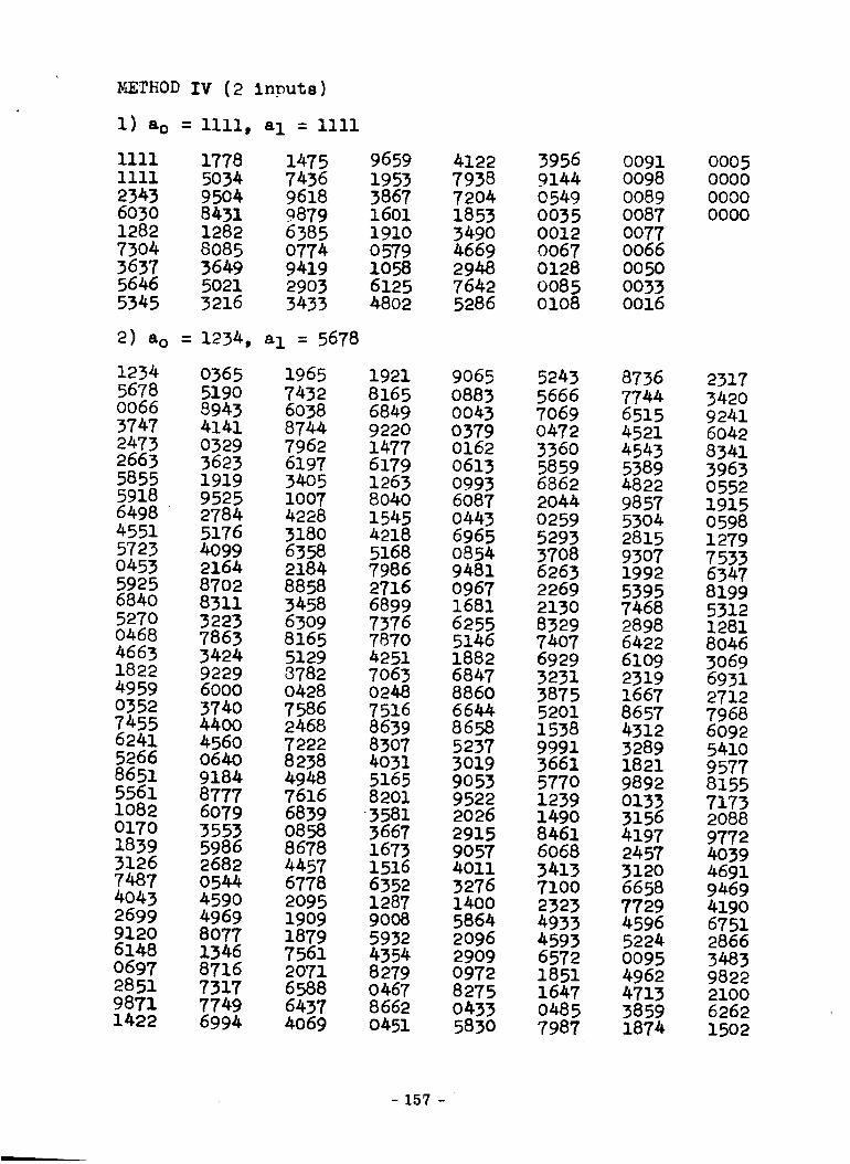
)_THOD IV (2 inputs)

i) ao = iiii, a I = iiii

iiii 1778 1475 9659 4122 3956 0091

IIii 5034 7436 1953 7938 9144 0098

2343 9504 9618 3867 7204 0549 0089

6030 8431 9879 1601 1853 0035 0087

1282 1282 6385 1910 3490 0012 0077

7304 8085 0774 0579 4669 0067 0066

3637 3649 9419 1058 2948 0128 0050

5646 5021 2903 6125 7642 0085 0033

5345 3216 3433 4802 5286 0108 0016

2) ao = 1234, a I = 5678

0005ooo0

0000

0000

1234 0365 1965 1921 9065 5243 8736 2317

5678 5190 7432 8165 0883 5666 7744 3420

0066 8943 6038 6849 0043 7069 6515 9241

3747 4141 8744 9220 0379 0472 4521 6042

2473 0329 7962 1477 0162 3360 4543 83412663 3623 6197 6179 0613 5859 5389 3963

5855 1919 3405 1263 0993 6862 4822 0552

5918 9525 1007 8040 6087 2044 9857 1915

6498 2784 4228 1545 0443 0259 5304 0598

4551 5176 3180 4218 6965 5293 2815 1279

5723 4099 6358 5168 0854 3708 9307 75330453 2164 2184 7986 9481 6263 1992 6347

5925 8702 8858 2716 0967 2269 5395 8199

6840 8311 3458 6899 1681 2130 7468 53125270 3223 6309 7376 6255 8329 2898 1281

0468 7863 8165 7870 5146 7407 6422 8046

4663 3424 5129 4251 1882 6929 6109 30691822 9229 8782 7063 6847 3231 2319 6931

4959 6000 0428 0248 8860 3875 1667 2712

0352 3740 7586 7516 6644 5201 8657 7968

7455 4400 2468 8639 8658 1538 4312 6092

6241 4560 7222 8307 5237 9991 3289 5410

5266 0640 8238 4031 3019 3661 1821 9577

8651 9184 4948 5165 9053 5770 9892 8155

5561 8777 7616 8201 9522 1239 0133 71731082 6079 6839 "3581 2026 1490 3156 2088

0170 3553 0858 3667 2915 8461 4197 9772

1839 5986 8678 1673 9057 6068 2457 4039

3126 2682 4457 1516 4011 3413 3120 46917487 0544 6778 6352 3276 7100 6658 9469

4043 4590 2095 1287 1400 2323 7729 4190

2699 4969 1909 9008 5864 4933 4596 6751

9120 8077 1879 5932 2096 4593 5224 2866

6148 1346 7561 4354 2909 6572 0095 3483

0697 8716 2071 8279 0972 1851 4962 9822

2851 7317 6588 0467 8275 1647 4713 2100

9871 7749 6437 8662 0433 0485 3859 6262

1422 6994 4069 0451 5830 7987 1874 1502

- 157 -

METHODZV (cont.)

4055 6909 5192 3767 6959 1209 5812 6086

0906 7367 5125 0141 3023 7264 9774 3681

6738 8986 6090 5311 0370 7812 6321 40251046 1998 2112 7488 1185 8117 5918 8160

0479 9540 8620 7687 4384 4830 4076 84/_0

5010 0609 2054 5602 1950 2051 1217 8704

3997 8098 7054 0625 5488 9063 9605 4617

0249 9316 4889 5012 7016 5882 6880 1863

9952 4409 4870 1325 5038 3085 0755 601447801 0742 8094 6409 3466 1459 1944 2040

5705 2714 4177 4919 4617 5010 4677 2685

2699 0137 8086 5258 0025 3095 0920 47743787 3718 7752 8641 1154 5059 3028 8181

7339 5093 6826 4242 0288 6576 7857 0560

1872 8357 9151 5278 3323 2679 7909 5813

7387 6552 4647 9223 9570 6171 1410 2552

8265 3070 5246 6789 8011 5321 1516 8347

0452 1146 3781 6149 6652 8358 1575 30157357 5182 8351 7455 2891 4729 0845 1662

3253 9385 5751 8407 2309 5249 1618 0109

9232 6330 0226 6741 6753 8225 3672 1811

3277 4070 5297 6175 5926 1730 9412 1973

5514 7631 4090 2658 0182 2292 5608 57310693 0581 6647 8484 0785 9651 7824

8212 4336 1862 5504 1428 1200 8769

- 158 -

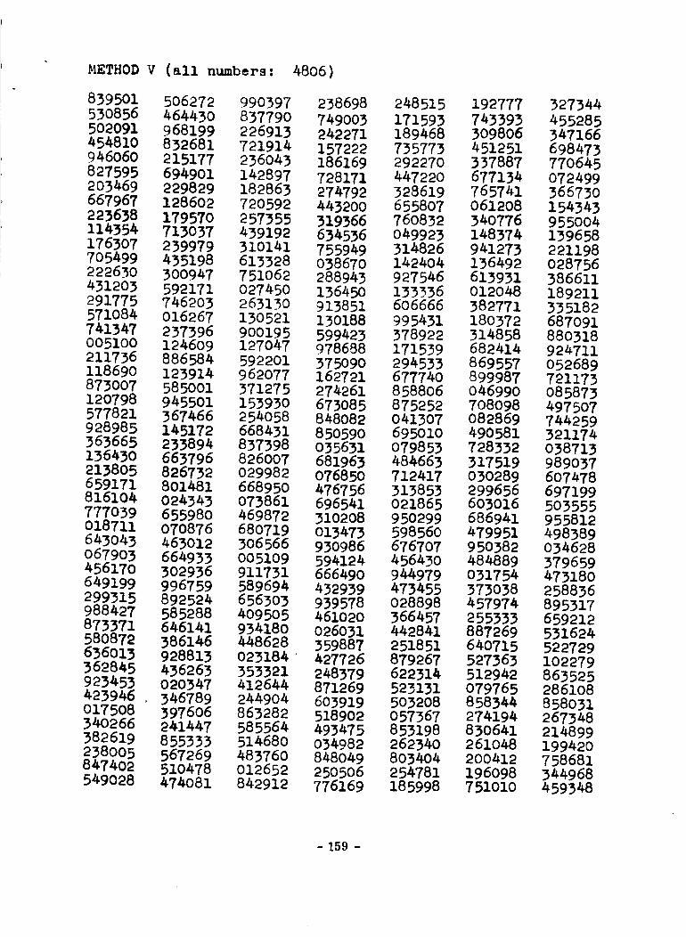
METHODV (all numbers: 4806)

839501

530856

502091

454810946060

827595

203469

667967

223638

114354

176307

705499

222630431203

291775571084

741347

OO51OO

211736118690

873007120798

577821

928985

365665

136430

213805

659171816104

777059018711

643043

067903456170

649199

299315988427

875371

580872636013

362845

923453423946

O17508

340266

582619

238005847402549028

506272 990397 238698 248515 192777 327344

464430 837790 749003 171593 743593 455285968199 226913 242271 189468 309806 347166

832681 721914 157222 735773 451251 698473

215177 236043 186169 292270 337887 770645

694901 142897 728171 447220 677134 072499

229829 182863 274792 328619 765741 366730128602 720592 443200 655807 061208 154343

179570 257355 319366 760832 340776 955004713037 439192 634536 049923 148374 139658

239979 310141 755949 314826 941273 221198

435198 613328 038670 142404 136492 028756

300947 751062 288943 927546 613931 386611

592171 027450 136450 133336 012048 189211

746203 263130 913851 606666 382771 335182

016267 130521 130188 995431 180372 687091

237396 900195 599423 378922 314858 880318

124609 127047 978688 171539 682414 924711

886584 592201 375090 294535 869557 052689

123914 962077 162721 677740 899987 721173

585001 371275 274261 858806 046990 085873

945501 153930 673085 875252 708098 497507

567466 254058 848082 041307 082859 744259145172 668431 850590 695010 490581 321174

233894 837398 035631 079853 728332 038715

663796 826007 681963 484663 317519 989037

826732 029982 076850 712417 030289 607478

801481 668950 476756 313853 299656 697199

024343 073861 696541 021865 603016 503555

655980 469872 310208 950299 686941 955812

070876 680719 013473 598560 479951 498389

463012 306566 930986 676707 950382 034628

664933 005109 594124 456430 484889 379659

302936 911731 666490 944979 031754 473180

996759 589694 432939 473455 573058 258836

892524 656303 939578 028898 457974 895517

585288 409505 461020 366457 255333 659212

646141 934180 026031 442841 887269 531624386146 448628 359887 251851 640715 522729

928813 023184" 427726 879267 527363 102279

436263 353321 248379 622314 512942 863525020347 412644 871269 523131 079765 286108

546789 244904 603919 503208 858344 858031

397606 863282 518902 057367 274194 267348241447 585564 493475 853198 830641 214899

855333 514680 034982 262340 261048 199420

567269 483760 848049 803404 200412 758681

510478 012652 250506 254781 196098 344968474081 842912 776169 185998 751010 459348

- 159 -

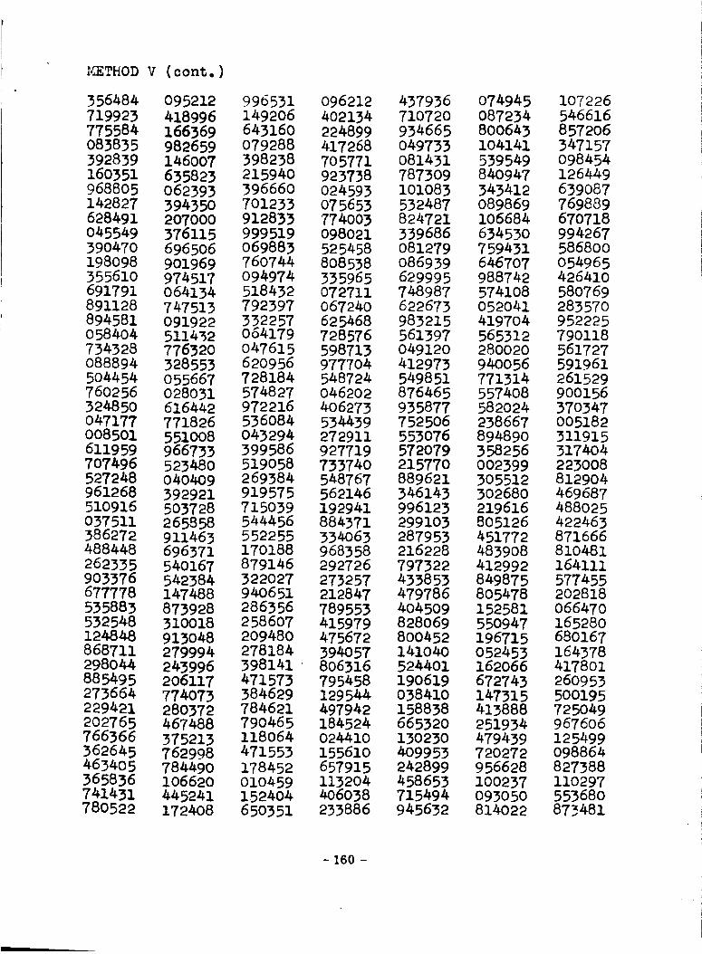
tI_THOD V (cont.)

356484

719923

775584

083835

392839

160351

968805

142827

628491

045549

390470

198098

35561O

691791

891128

894581

058404

734328

088894

504454

760256

324850

047177

008501

611959

7O7496

527248961268510916037511

386272488448262335903376

677778

555883

532548124848

868711298044

885495273664

229421

202765766366

362645

463405365836

741431

780522

095212

418996

166369

982659

146007

635823

062393

394350

207000

376115

696506901969

974517064134

747513

091922

5114_2776320

328553

055667

028031616442

771826

5510o8

966733

523480

040409

392921

503728

265858

911463

696371

540167

542384147488

873928

310018

913o48279994

243996206117

774073

280372467488

375213762998

784490

106620

445241

172408

996531

149206

643160

079288

398238

215940

396660

701233

912833

999519

o69883

760744

094974

518432

792397

332257064179

o47615

620956

728184

574827

972216

536084

043294

399586

519058

269384

919575

715039

544456

552255170188

879146

322027

940651

286356

258607

209480

278184

398141

471573

384629

784621

790465118064

471553

178452

010459

152404

650351

096212

402134

224899

417268

7O5771

923738

024593

075653

774003

098021

525458

8O8538

335965072711

067240

625468

728576

598713

977704

548724

046202

406273

534439

272911

927719

733740

548767

562146

192941

884371

334063968358

292726

273257212847

789553415979

475672

394057

• 8O6316

795458

129544

497942

184524024410

155610

657915

113204406038

233886

437936

71072O

934665

049733

081431

787309

101083

532487

824721

339686

081279

086939

629995

748987

622673

983215

561397

049120

412973

549851

876465

935877

752506

553076572079

215770

889621

346143

996123

299103

287953216228

797322

433853

479786

4O45O9

828069

800452141040

524401

190619

038410

158838

665320

130230

409953242899458653715494

945632

074945

O87234

800643

I04141

539549

84O947

343412

089869

106684

634530

759431

646707

988742

574108

052041

419704

56531228002094O056

771314

557408

582024

238667

894890

358256002399305512

302680219616

805126

451772

483908412992

849875

8O5478

152581

550947

196715

052453162066

672743

147315413888

251934

479439

720272

956628

10O237O93050814022

1O7226

546616

857206347157

098454126449

639O87769889

670718

994267

586800

054965426410

580769

283570

952225

790118

561727

591961

261529

900156

370347

005182

311915

3174O4

223008812904

469687

488025

422463871666

810481

164111

577455202818

066470

165280

680167

164378

4178O1

260953

500195

725049

9676O6

125499098864

827388

110297

553680873481

- 160 -

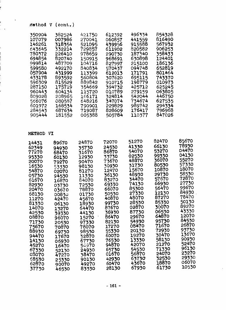
Method V (cont.)

350904107079146261643645780372694854999814599580057904433178596309287150960443809028566076601972284543905444

3825240079863183543322142264108207404877094921704319998935928155291757196o41342o8965

080587

168534

687634

181552

42175O

270041

521O95

729857

978659

150915104716

840834

113399

560804

889842354669

115720166171648216

790901

719087

005388

612392

060857

439956

611902

290730

968691

827997

570437

612013

30762O

910715

394732

010789

324814

347074

229829828609505784

496534

441559

915588

820582

187340

630898

215100094748

171791

695115

198779

425712

279159

542044

734674989742

176417

i10377

854328

816490

567952

906253

358433124401

186136

652819801464

743370

010973

625245063805

446750627535

294334796968

847026

METHOD VI

14431

6234977270

9533O2O07O

16530

54870

0573061670

82930204706813011270

81330

14070

42530

08870

71730

7567O

88930

94470

14130

45270

6733O

OS070

685306287O

37730

8967O

94930

68470

60130

7927O

53330

0207094530

16870

03730

03670

0083o42470

06130

13270

3933096070

2053070870

6973O

17670

0693O

1647O

5213047270

25330

9OO7O46530

24870

357303167012930

90470

981308127O

11330

84070

72530

78870

01730

4567O

1893O

64470

44130

152709733078o7098530

3287O67730

5697O

2493O

38470

90130

4927O8333O

72070

2453O8687O

3373073670

30930

1247O

36130

832706933066070

50530

40870

99?3O

87670

369308647O

82130

17270

55330

60070

76530

94870

6573001670

4293060470

28130

51270

41330

54070

025304887O

3173Oi5670

48930

34470

74130

85300

2733048O7O

2853002870

877302967O5493008470

20130

19270

133304207054530

56870

6373(_

436706793O

8247O

6613O

53270993303607080530lO870

2973O

57670

6693O

5647o

1213087270

85330

30070065306487O

95730

71670

7293o

3047058130

21270

71330

240703253018870

61730

8567O

78930

04470

04130

5527O

5733O

18070

585307287O

27730

996?0

84930.

7847o

501308927O433301207084530

2687093730

13670

90930

5247096130

23270

29330

06070

10530

- 161 -

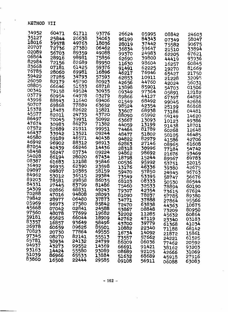
PIETHOD VII

34952

35127

18016

20707

02O8906864

82984

83668

76785

59422

26050

08805

00341

03779

43996

50707

15378

45577

86497

47674

07572

4643746580

46992

87054

58458

54028

08387

36492

09897

84962

892o3

84331

5430970288

79842

O5969

45668

97560

59181

83357

26978

70823

9734565781

94937

93163

5103983860

60471

25844

39578

72736

56703

28916

72156

071812806027285

8217966646

79158

60954

88943698681848382011

70045

30983

52689

33942

59189

96902

42439

5624766194

61683

9693509807

5301278581

2744502866

47016

28977

96973

07042

48078656251685760659

2073008270

38934

4327314424

86966

16508

61711

26638

49763

27380

8935998981

82689

6142569981

3479345790

5153349524

6497811640

7788982622

24735

3993186279

21911

13521

46571

8831266246

0373428020

12188

62390

10385

36515

2985883799

68831

9480806480

2758002841

7769966044

9364909626

77864

82141

24132

99552555806553322444

93776

34063

18036

06462

49088

75856

8995O

59376

16896

57593

80923

68718

30935

0327969406

63652

1582143720

5099271382

9995109244

40438

98913

14436

09224

67434

95846

23598

58159

29384

8603581486

49243

28093

37873858422458819682189095849685501

49555

55513

24799

14569

93O8913884

29585

26624

96199

28019

36834

99370

62690

11630

91491

46217

62853

42656

13898

09349

89866

01549

98524

3360788O9O

63667

4405974464

4847794822628632831894862

18798

00536

13176

59470

73549

68103

75460

79307

81090

34771

7247o

53867

3220242762

43700

10882

16734

73557

86oo9

66691

o8689

5163209108

05995

84343

37442

59647

24983

39800

98604

6222576946

io911

44760

85901

97364

44127

68492

42354

68938

65992

130931319981789

51802

8297927146

3099698692

15244

9599246336

57850

5339508333

3253342354

78O37

37888

63838O8848

11285

47119

39779

2234014092

57662

O6O36

91421

9210568689

56911

08842

07349

75582

21510

62205

44419

16257

19270

6542721228

42024

547O3

05891

67397

99045

25199

73186

5q149

10123

9143860268

50105

41586

0896577184

21676

89967

537513938O

24945

58747

5053078894

73615

57785

27864

44363

73209

45632

2334061368

71188

2187224221

77462

3816242666

4591806O88

24603

58047

90675

33894

67621

93936

6O845

81669

217503209_

56031

o15o612182

64898

42686

86868

04481

14620

49386

1870112648

46485

4270661608

54742

93469

6978352015

42675

96763

56676

86544

6019O67624

89580

95566

10675

8095060864

03183

41034

68142

15861

61525

20592

9320331069

27916

63083

- 162 -

BIBLI OG.WAPHY

i. IBM Reference Manual, Random Number Generation and

Testing, International Business Machine Corporation,

1959.

2. The RAND Corporation, A Million Random Digits with

lO0,O00 Norma I Deviates, The Free Press, Glencoe,

Illinois, 1955.

3. _4. G. KENDALL and B. Babin6ton SMITH, Randomness and

Random Samplln6 Numbers, Journal of the Royal Statistical

Society, Vol. lOl, Part 1 (1938) pp.147 - 166.

4. F. MOSTELLER, R. ROURKE, and G. THOMAS, Jr., Probability

with Statistical Applications, Addison Wesley Publishing

Co., 1961.

5. S. H. HOLLINGDALE, High Speed Computing, The Mac Millan

Co., New York, 1959,

6. Georse E. FORSYTHE, Generation and Testin5 of Random

Di6its at the National Bureau of Standards, The Monte

Carlo Method, The National Bureau of Standards Applied

Mathematics Series, Los Anseles, No. 4, 1951, Pp. 34 - 35.

7. D. H. LE_MER, Mathematical Meth@_ in Lar_e-Scale

Computing Unite, Proceedinss of the 2rid Symposium on

Large Scale Digital Calculatln_ Machinery, Harvard

University Press, 1951, pp. i_I - 146.

8. H. GRIFFIN, Elementary Theory of Numbers, Mc Graw-Hill

Book Co. Inc., New York, 1954, pp. 53 - 65.

- 163 -

9. J. F. KENNEY and E. S. KEEPING, Mathematlcs 9f Statistics

Part I, D. Van Nostrand Company Inc., Princeton, New

Jersey, 1957.

i0. Hugh D. YOUNG, Statlati_l Treatment of Zxperimental

Data, Mc Graw-Hill Book Company, Inc., New York, 1962.

Ii. Bernice BROWN, Some Tes%s of the Randomness of a Million

Random Digits. RAOP-44, The RAND Corporation, Santa

Monica, California, 1948.

These sources also were used:

12. Bernard A. GALLER, The Language of Computers, The Mc

Graw-Hill Book Co. Inc., 1959.

13. G. R. STIBITZ and J. A. LARRIVEE, ;_athematics and

Cgmputers, Mc Graw-Hill Book Company Inc., 1957.

14. Howard W. ALEXANDER, Elements 0fMathemat_cal Statistics,

John Wiley and Sons Inc., 1961.

15. J. M. CAMERON, Results on Some Tests of Randomness on

Pseudo-Random Numbers, Annals of Mathematical Statistics

23, 1952, pp. 138.

16. _. J. COCHRAN, Th_ x2 Test of _oodneas of Fit, Annals

of Mathematical Statistics 23, 1952, pp. 315 - 345.

17. B. LXNDGREN and G. MC ELRATH, Introductlon to Probabillty

and Stati@tlcs, The Mac Mlllan Company, 1959.

18. Herbert A. MEYER (Ed), SymDoslum on Monte Carlo Methods,

John Wiley and Sons, Inc., 1956, Bibliography.

19. D. D. MC CRACKEN, The Monte Carlo Method, Scientific

America, Vol. 192, May 1955, pp. 90 - 96.

- 164 -

SectionVII Future Plans

1. Judging from the number of requests for reprints of the Bibliography

on Computer-Aided Circuit Analysis and Design compiled earlier this year, it seems

there is an existing demand for such a reference in various quarters. Continuous atten-

tion will be given to newly published literature so that the Bibliography may be updated

by bringing in additibnal entries from time to time.

2. The time-sharing computer service provided by General Electric Company

on the Villanova University campus has been used by graduate and undergraduate

students to solve various types of problems ranging from the relatively short ones

connected with simple laboratory experiments through more complicated and lengthy

thesis problems. This research project is particularly interested in the use of a

circuit analysis program developed by the General Electric staff called STANPAK

(_Statistical Tolerance An__.alysis Package ). It is basically a reliability prediction and

tolerance analysis and adjustment program using the statistical approach. It handles

the steady states only and has not been extended to transient computations. Because

of incomplete knowledge about the program and the peculiar limitations of the Desk

Size Computer at the input terminal, the program has not been managed to smooth

operation yet. Further effort will be made in the study and evaluation of the STANPAK

in the coming months.

3. In the process of circuit design there is a stage of parameter optimization

after the circuit geometry has been chosen. Instead of numerical values available for

analysis, the circuit components and other parameters such as frequency may be

represented by symbols. Nonnumerical manipulation by the digital computer is a vast

- 165 -

area to be explored. The practical programs written for symbolic manipulation are

far sparse than theoretical dissertation published on the subject. Techniques will be

attempted for efficient manipulation of mathematical symbols. Again the interest will

be centered around the computer size of the same order as IBM 1620 with a disk file.

4. In the manual solution of the transient response of electric circuits, the

frequency domain approach by Laplace transform is always a favorable one. Several

recent research papers were published in the new methods of finding: the inverse

of the Lapalce transforms. An attempt will be made, using the digital computer as

an aid, to evaluate and compare various approaches for accuracy, time and storage

requirements for computation, and the ease with which these methods may be applied

to various types of electronic circuits.

- 166 -

Documents

N66 3! - NASA · meetings on the subject is the session on "Computers in Network ... W. Mayeda and M. E. Van Valkenberg, "Network Analysis and ... Chapter 26, pp. 280-290