N5615_1

StatisticalSignal

ProcessingECE 5615 Lecture Notes

Spring 2013

© 2007–2013Mark A. Wickert

Equalizer+1

-1

DistortedInput

EqualizedInput

EstimatedData

x[n]

e[n]

y[n]

-+

d[n]

.

Chapter 1Course Introduction/Overview

Contents

1.1 Introduction . . . . . . . . . . . . . . . . . . . . . . . 1-31.2 Where are we in the Comm/DSP Curriculum? . . . . 1-41.3 Instructor Policies . . . . . . . . . . . . . . . . . . . . 1-51.4 The Role of Computer Analysis/Simulation Tools . . . 1-61.5 Required Background . . . . . . . . . . . . . . . . . . 1-71.6 Statistical Signal Processing? . . . . . . . . . . . . . . 1-81.7 Course Syllabus . . . . . . . . . . . . . . . . . . . . . 1-91.8 Mathematical Models . . . . . . . . . . . . . . . . . . 1-101.9 Engineering Applications . . . . . . . . . . . . . . . . 1-121.10 Random Signals and Statistical Signal Processing in

Practice . . . . . . . . . . . . . . . . . . . . . . . . . . 1-13

1-1

CHAPTER 1. COURSE INTRODUCTION/OVERVIEW

.

1-2 ECE 5615/4615 Statistical Signal Processing

1.1. INTRODUCTION

1.1 Introduction

✏ Course perspective

✏ Course syllabus

✏ Instructor policies

✏ Software tools for this course

✏ Required background

✏ Statistical signal processing overview

ECE 5615/4615 Statistical Signal Processing 1-3


1.2 Where are we in the Comm/DSPCurriculum?

ECE 3205 Signals & Systems II

ECE 2205 Signals & Systems I

ECE 2610 Signals & Systems

ECE 3610 Eng. Prob.

& Stats.

ECE 4670 Comm.

Lab

ECE 4680 DSP Lab

ECE 5625 Comm.

Systems I

ECE 5630 Comm.

Systems II

ECE 5675 PLL & Applic.

ECE 5610 Random Signals

ECE 6640 Spread

Spectrum

ECE 5720 Optical Comm.

Coding Thy, Image Proc, Sat. Comm, Radar Sys

ECE 5635 Wireless Comm.

ECE 6620 Detect. &

Estim. Thy.

ECE 6650 Estim. &

Adapt. Fil.

ECE 5650 Modern

DSP

ECE 5655 Real-Time

DSP

ECE 5615 Statistical

Signal Proc

Courses Offered According to Demand

You are Here!

ECE 5685Wireless

Networking


1.3. INSTRUCTOR POLICIES

1.3 Instructor Policies

✏ Working homework problems will be a very important aspectof this course

✏ Each student is to his/her own work and be diligent in keepingup with problems assignments

✏ Homework papers are due at the start of class

✏ If work travel keeps you from attending class on some evening,please inform me ahead of time so I can plan accordingly, andyou can make arrangements for turning in papers

✏ The course web site

http://www.eas.uccs.edu/wickert/ece5615/

will serve as an information source between weekly class meet-ings

✏ Please check the web site updated course notes, assignments,hints pages, and other important course news; particularly ondays when weather may result in a late afternoon closing of thecampus

✏ Grading is done on a straight 90, 80, 70, ... scale with curvingbelow these thresholds if needed

✏ Homework solutions will be placed on the course Web site inPDF format with security password required; hints pages mayalso be provided



1.4 The Role of Computer Analysis/Simulation Tools

✏ In working homework problems pencil and paper type solu-tions are mostly all that is needed

– It may be that problems will be worked at the board bystudents

– In any case pencil and paper solutions are still required tobe turned in later

✏ Occasionally an analytical expression may need to be plotted,here a visualization tool such as MATLAB or Mathematicawill be very helpful

✏ Simple simulations can be useful in enhancing your under-standing of mathematical concepts

✏ The use of MATLAB for computer work is encouraged sinceit is fast and efficient at evaluating mathematical models andrunning Monte-Carlo system simulations

✏ There will be one or more MATLAB based simulation projects,and the Hayes text supports this with MATLAB based exer-cises at the end of each chapter


1.5. REQUIRED BACKGROUND

1.5 Required Background

✏ Undergraduate probability and random variables (ECE 3610 orsimilar)

✏ Linear systems theory

– A course in discrete-time linear systems such as, ECE5650 Modern DSP, is highly recommend (a review is pro-vided in Chapter 2)

✏ Familiarity with linear algebra and matrix theory, as matrix no-tation will be used throughout the course (a review is providedin Chapter 2)

✏ A familiarity with MATLAB as homework problems will re-quire its use, and a reasonable degree of proficiency will allowyour work to proceed quickly

✏ A desire to dig in!



1.6 Statistical Signal Processing?

✏ The author points out that the text title is not unique, in factA Second Course in Discrete-Time Signal Processing is alsoappropriate

✏ The Hayes text covers:

– Review of discrete-time signal processing and matrix the-ory for statistical signal processing

– Discrete-time random processes– Signal modeling– The Levinson and Related Recursions– Lattice Filters– Wiener and Kalman filtering– Spectrum estimation– Adaptive filters

✏ The intent of this course is not entirely aligned with the texttopics, as this course is also attempting to fill the void leftby Random Signals, Detection and Extraction of Signals from

Noise, and Estimation Theory and Adaptive Filtering

✏ During the Spring 2011 offering of this course, a reasonabletopic coverage was arrived at and serves as the guidelines forthe Spring 2013 offering

✏ Two Steven Kay books on detection and estimation are nowoptional texts, and may take the place of the Hayes book in thefuture


1.7. COURSE SYLLABUS

1.7 Course Syllabus

ECE 5615/4615Statistical Signal Processing

Spring Semester 2013

Instructor: Dr. Mark Wickert Office: EN292 Phone: [email protected] Fax: 255-3589http://www.eas.uccs.edu/wickert/ece5615/

Office Hrs: Monday 3:30–4:30 PM, 7:20–8:00 PM, other times by appointment.

Required Texts:

Monson H. Hayes, Statistical Digital Signal Processing and Modeling, JohnWiley, 1996.

Optional Texts:

Steven Kay, Fundamentals of Statistical Signal Processing, Vol I: EstimationTheory, Vol II: Detection Theory, Prentice Hall, 1993/1998. ISBN-978-0133457117/978-0135041352 Harry L. Van Trees, Detection, Estimation, andModulation Theory, Part I, Wiley-Interscience, 2001 (reprint of 1968 edition).

Optional Software:

MATLAB Student Version with Simulink with MATLAB 7.x, Simulink 5.x,and Symbolic Math Toolbox. An interactive numerical analysis, data analysis,and graphics package for Windows/Linux/Mac OSX $99.95. Order fromwww.mathworks.com/student. Note: The ECE PC Lab has the full ver-sion of MATLAB and Simulink for windows (ver. 7.x) with many toolboxes.

Grading: 1.) Graded homework assignments and computer projects worth 55%.2.) Midterm exam worth 20%.3.) Final exam worth 25%.

Topics Text Sections

1. Introduction and course overview Notes ch 1

2. Background: discrete-time signal processing, linear algebra 2.1–2.4 (N ch2)

3. Random variables & discrete-time random processes 3.1–3.7 (N ch3)

4. Classical detection and estimation theory N ch4(optional texts)

5. Signal modeling 4.1–4.8 (N ch5)

6. The Levinson recursion 5.1–5.5 (N ch6)

7. Optimal filters including the Kalman filter 7.1–7.5 (N ch8)

8. Spectrum estimation 8.1–8.8 (N ch9)

9. Adaptive filtering 9.1–9.4(N ch10)



1.8 Mathematical Models

✏ Mathematical models serve as tools in the analysis and designof complex systems

✏ A mathematical model is used to represent, in an approximateway, a physical process or system where measurable quantitiesare involved

✏ Typically a computer program is written to evaluate the math-ematical model of the system and plot performance curves

– The model can more rapidly answer questions about sys-tem performance than building expensive hardware pro-totypes

✏ Mathematical models may be developed with differing degreesof fidelity

✏ A system prototype is ultimately needed, but a computer sim-ulation model may be the first step in this process

✏ A computer simulation model tries to accurately represent allrelevant aspects of the system under study

✏ Digital signal processing (DSP) often plays an important rolein the implementation of the simulation model

✏ If the system being simulated is to be DSP based itself, the sim-ulation model may share code with the actual hardware proto-type


1.8. MATHEMATICAL MODELS

✏ The mathematical model may employ both deterministic andrandom signal models

FormulateHypothesis

Define Experiment toTest Hypothesis

Physicalor Simulation ofProcess/System

Model

SufficientAgreement?

All Aspectsof Interest

Investigated?

Stop

No

No

Observations Predictions

Modify

The Mathematical Modeling Process1

1Alberto Leon-Garcia, Probability and Random Processes for Electrical Engineering,



1.9 Engineering Applications

Communications, Computer networks, Decision theory and decisionmaking, Estimation and filtering, Information processing, Power en-gineering, Quality control, Reliability, Signal detection, Signal anddata processing, Stochastic systems, and others.

Relation to Other Subjects2

!andom Signalsand Systems

Pro2a2ility

Estimationand Filtering

SignalProcessing

!elia2ility

DecisionTheory

9ameTheory

:inearSystems

;ommunication= >ireless

InformationTheory

!andomAaria2les

Bthers

Mathematics

Statistics

Addison-Wesley, Reading, MA, 19892X. Rong Li, Probability, Random Signals, and Statistics, CRC Press, Boca Raton, FL, 1999


1.10. RANDOM SIGNALS AND STATISTICAL SIGNAL PROCESSING IN PRACTICE

1.10 Random Signals and Statistical Sig-nal Processing in Practice

✏ A typical application of random signals concepts involves oneor more of the following:

– Probability

– Random variables

– Random (stochastic) processes

Example 1.1: Modeling with Probability

✏ Consider a digital communication system with a binary sym-

metric channel and a coder and decoder

!

"

!

"

Input (utput" !–

" !–

!

!

CoderBinaryChannel Decoder

BinaryChannelModel

Communication!System!with!Error!Control

BinaryInformation

ReceivedInformation

! Error!Pro-a-ility=

A data link with error correction



✏ The channel introduces bit errors with probability Pe.bit/ D ✏

✏ A simple code scheme to combat channel errors is to repetition

code the input bits by say sending each bit three times

✏ The decoder then decides which bit was sent by using a major-

ity vote decision rule

✏ The system can tolerate one channel bit error without the de-coder making an error

✏ The probability of a symbol error is given by

Pe.symbol/ D P.2 bit errors/ C P.3 bit errors/

✏ Assuming bit errors are statistically independent we can write

P.2 bit errors/ D ✏ � ✏ � .1 � ✏/ C ✏ � .1 � ✏/ � ✏

C .1 � ✏/ � ✏ � ✏ D 3✏2.1 � ✏/

P.3 errors/ D ✏ � ✏ � ✏ D ✏3

✏ The symbol error probability is thus

Pe.symbol/ D 3✏2� 2✏3

✏ Suppose Pe.bit/ D ✏ D 10�3, then Pe.symbol/ D 2:998 ⇥

10�6

✏ The error probability is reduced by three orders of magnitude,but the coding reduces the throughput by a factor of three



Example 1.2: Separate Queues vs A Common Queue

A well known queuing theory result3 is that multiple servers, witha common queue for all servers, gives better performance than mul-tiple servers each having their own queue. It is interesting to seeprobability theory in action modeling a scenario we all deal with inour lives.

!

"

m

...

Servers

(ne*ueue

,-aiting line4

Departing7ustomers

:ate

!

Ts

= Average ServiceTime

!

"

m

...

ServersSeparate*ueues

Departing7ustomers

:ate

! m!Ts

= Average ServiceTime

:andomArrivals atper unit time,exponentiallydistriAuted4

!

:andomArrivals atper unit time,exponentiallydistriAuted4

!

7ustomers

7ustomers

(ne long serviceBtime customer forces those Aehind into a long -ait

Assume customersrandomly picE Fueues

Common queue versus separate queues3Mike Tanner, Practical Queuing Analysis, The IBM-McGraw-Hill Series, New York, 1995.



Common Queue Analysis

✏ The number of servers is defined to be m, the mean customerarrival rate is � per unit of time, and the mean customer servicetime is Ts units of time

✏ In the single queue case we let u D �Ts D traffic intensity

✏ Let ⇢ D u=m D server utilization

✏ For stability we must have u < m and ⇢ < 1

✏ As a customer we are usually interested in the average time inthe queue, which is defined as the waiting time plus the servicetime (Tanner)

TCQQ D Tw C Ts D

Ec.m; u/Ts

m.1 � ⇢/C Ts

D

⇥Ec.m; u/ C m.1 � ⇢/

⇤Ts

m.1 � ⇢/

where

Ec.m; u/ D

um=mä

um=mä C .1 � ⇢/Pm�1

kD0 uk=kä

is known as the Erlang-C formula

✏ To keep this problem in terms of normalized time units, wewill plot TQ=Ts versus the traffic intensity u D �Ts

✏ The normalized queuing time is

TCQQ

Ts

D

Ec.m; u/ C .m � u/

m � uD

Ec.m; u/

m � uC 1



Separate Queue Analysis

✏ Since the customers randomly choose a queue, arrival rate intoeach queue is just �=m

✏ The server utilization is ⇢ D .�=m/ � Ts which is the same asthe single queue case

✏ The average queuing time is (Tanner)

TSQQ D

Ts

1 � ⇢D

Ts

1 ��Ts

m

D

mTs

m � �Ts

✏ The normalized queuing time is

TSQQ

Ts

D

m

m � �Ts

D

m

m � u

✏ Create the Erlang-C function in MATLAB:

function Ec = erlang_c(m,u);

% Ec = erlangc(m,u)

%

% The Erlang-C formula

%

% Mark Wickert 2001

s = zeros(size(u));

for k=0,

s = s + u.^k/factorial(k);

end

Ec = (u.^m)/factorial(m)./(u.^m/factorial(m) + (1 - u/m).*s);

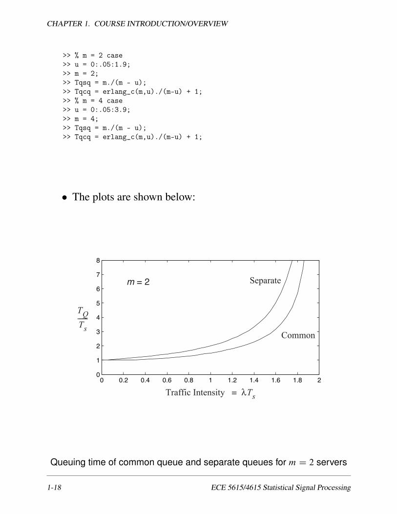
✏ We will plot TQ=Ts versus u D �Ts for m D 2 and 4



>> % m = 2 case

>> u = 0:.05:1.9;

>> m = 2;

>> Tqsq = m./(m - u);

>> Tqcq = erlang_c(m,u)./(m-u) + 1;

>> % m = 4 case

>> u = 0:.05:3.9;

>> m = 4;

>> Tqsq = m./(m - u);

>> Tqcq = erlang_c(m,u)./(m-u) + 1;

✏ The plots are shown below:

! !"# !"$ !"% !"& ' '"# '"$ '"% '"& #!

'

#

(

$

)

%

*

&

TQ

Ts

!!!!!!!

Traffic Intensity !Ts

=

Separate

Common

m , #

Queuing time of common queue and separate queues for m D 2 servers



! !"# $ $"# % %"# & &"# '!

$

%

&

'

#

(

)

*

TQ

Ts

!!!!!!!

Traffic Intensity !Ts

=

Separate

Common

m , '

Queuing time of common queue and separate queues for m D 4 servers

Example 1.3: Power Spectrum Estimation

✏ The second generation wireless system Global System for Mo-

bile Communications (GSM), uses the Gaussian minimum shift-keying (GMSK) modulation scheme

xc.t/ D

p2Pc cos

2⇡f0t C 2⇡fd

1X

nD�1

ang.t � nTb/

�

where

g.t/ D

1

2

⇢erf

�

r2

ln 2⇡BTb

✓t

Tb

�

1

2

◆ �

C erfr

2

ln 2⇡BTb

✓t

Tb

C

1

2

◆ ��



✏ The GMSK shaping factor is BTb D 0:3 and the bit rate isRb D 1=Tb D 270:833 kbps

✏ We can model the baseband GSM signal as a complex randomprocess

✏ Suppose we would like to obtain the fraction of GSM signalpower contained in an RF bandwidth of B Hz centered aboutthe carrier frequency

✏ There is no closed form expression for the power spectrum of aGMSK signal, but a simulation, constructed in MATLAB, canbe used to produce a complex baseband version of the GSMsignal

>> [x,data] = gmsk(0.3, 10000, 6, 16, 1);

>> [Px,F] = psd(x,1024,16);

>> [Pbb,Fbb] = bb_spec(Px,F,16);

>> plot(Fbb,10*log10(Pbb)); axis([-400 400 -60 20]);

Fre$uency in +H-

Spectr

al D

ensity 5

d7

8

GSM Baseband Power Spectrum

B

Pfraction

9:;; 9<;; 9=;; 9>;; ; >;; =;; <;; :;;9?;

9@;

9:;

9<;

9=;

9>;

;

>;

=;



✏ Using averaged periodogram spectral estimation we can esti-mate SGMSK.f / and then find the fractional power in any RFbandwidth, B , centered on the carrier

Pfraction D

R B=2

�B=2SGMSK.f / df

R1

�1SGMSK.f / df

– The integrals become finite sums in the MATLAB calcu-lation

! "! #!! #"! $!! $"! %!!!

!&$

!&'

!&(

!&)

#

B 200 kHz= 95.6%!

B 100 kHz= 67.8%!

B 50 kHz= 38.0%!

*F -and1idth in 5H7

Fra

ctional P

o1

er

GSM Power Containment vs. RF Bandwidth

Fractional GSM signal power in a centered B Hz RF bandwidth

✏ An expected result is that most of the signal power (95%) iscontained in a 200 kHz bandwidth, since the GSM channelspacing is 200 kHz



Example 1.4: A Simple Binary Detection Problem

✏ Signal x is measured as noise alone, or noise plus signal

x D

(n; only noise for hypothesis H0

V C n; noise + signal for hypothesis H1

✏ We model x as a random variable with a probability density

function dependent upon which hypothesis is present

0 VV 1– 1 V 1+1–

X

pxX H

0( ) p

xX H

1( )

VT

A!Two!HypothesisScenario

✏ We decide that the hypothesis H1 is present if x > VT , whereVT is the so-called decision threshold

✏ The probability of detection is given by

PD D Pr.x > VT jH1/ D

Z1

VT

px.X jH1/ dX

0 VV 1! 1 V 1"1!

X

pxX H

1! "

VT

PD

Pr x vTH1

#! "#

Area corresponding to PD



✏ We may choose VT such that the probability of false alarm,defined as

PF D Pr.x < VT jH0/ D

Z1

VT

px.X jH0/ dX

is some desired value (typically small)

0 VV 1! 1 V 1"1!

X

pxX H

0! "

VT

PF

Pr x vTH0

#! "#

Area corresponding to PF

Example 1.5: A Waveform Estimation Theory Problem

✏ Consider a received phase modulated signal of the form

r.t/ D s.t/ C n.t/ D Ac cos.2⇡fct C ✓.t// C n.t/

where ✓.t/ D kpm.t/, kp is the modulator phase deviationconstant, m.t/ the modulation, and n.t/ is additive white Gaus-sian noise

✏ The signal we wish to estimate is m.t/, information phasemodulated onto the carrier



✏ We may choose to develop an estimation procedure that ob-tains Om.t/, the estimate of m.t/ such that the mean square erroris minimized, i.e.,

MSE D Efjm.t/ � Om.t/j2g

✏ Another approach is maximum likelihood estimation

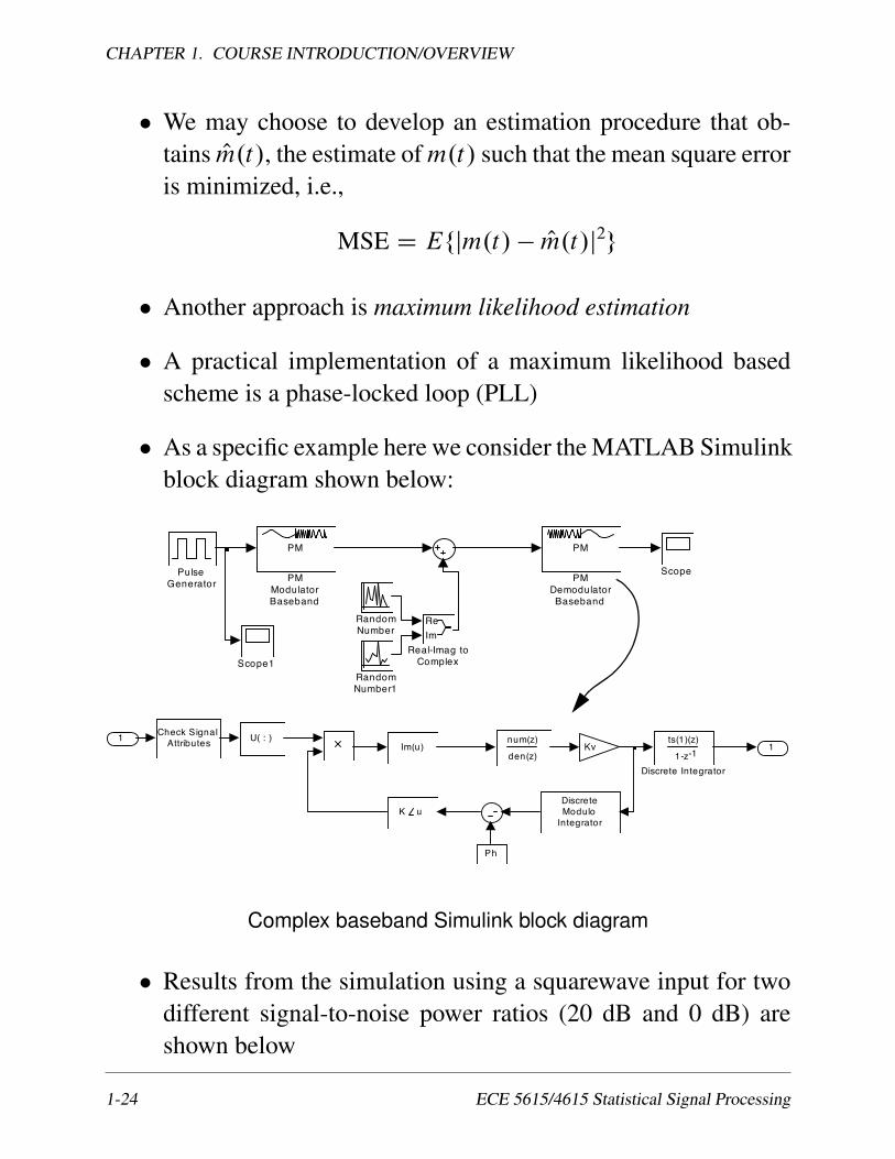
✏ A practical implementation of a maximum likelihood basedscheme is a phase-locked loop (PLL)

✏ As a specific example here we consider the MATLAB Simulinkblock diagram shown below:

Scope1

Scope

ReIm

Real-Imag toComplex

RandomNumber1

RandomNumber

PulseGenerator

PM

PMModulatorBaseband

PM

PMDemodulatorBaseband

1Kv

K u

num(z)

den(z)

DiscreteModulo

Integrator

1-z -1ts(1)(z)

Discrete Integrator

U( : )

Ph

Im(u)Check Signal

Attributes1

Complex baseband Simulink block diagram

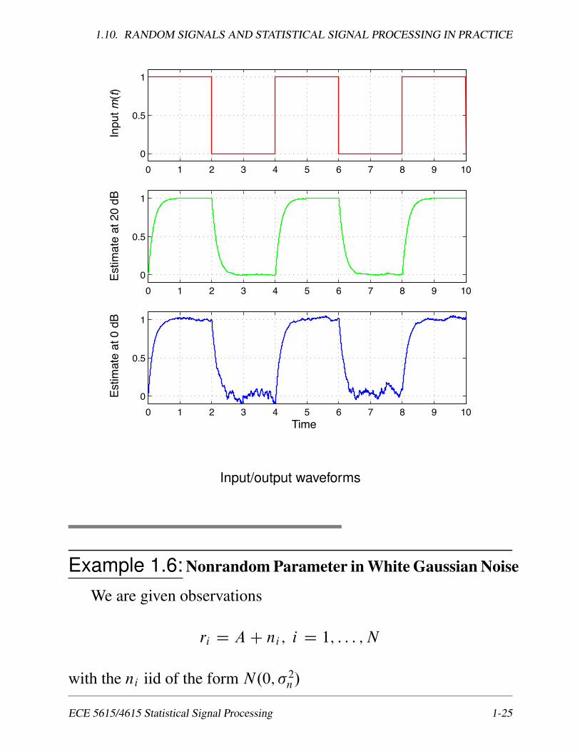
✏ Results from the simulation using a squarewave input for twodifferent signal-to-noise power ratios (20 dB and 0 dB) areshown below



0 1 2 3 4 5 6 7 8 9 100

0.5

1

0 1 2 3 4 5 6 7 8 9 100

0.5

1

0 1 2 3 4 5 6 7 8 9 100

0.5

1

Time

Inpu

t m(t)

Estim

ate

at 2

0 dB

Estim

ate

at 0

dB

Input/output waveforms

Example 1.6: Nonrandom Parameter in White Gaussian Noise

We are given observations

ri D A C ni; i D 1; : : : ; N

with the ni iid of the form N.0; �2n/



✏ The joint pdf is

prja.RjA/ D

NY

iD1

1p

2⇡�2n

exp�

.Ri � A/2

2�2n

�

✏ The log likelihood function is

ln prja.RjA/ç D

N

2ln

✓1

2⇡�2n

◆�

1

2�2n

NX

iD1

.Ri � A/2

✏ Solve the likelihood equation

@ lnŒprja.RjA/ç

@A

ˇ̌ˇ̌ADOaml

D

1

�2n

NX

iD1

.Ri � A/

ˇ̌ˇ̌ADOaml

D 0

H) Oaml D

1

N

NX

iD1

Ri

✏ Check the bias:

Ef Oaml.r/ � Ag D E

⇢1

N

NX

iD1

ri � A

�

D

1

N

NX

iD1

Efrig„ƒ‚…A

�A D 0

No Bias!



Example 1.7: Sat-Com Adaptive Equalizer

✏ Wideband satellite communication channels are subject to bothlinear and non-linear distortion

UplinkChannel

Transmitter

Transponder

Receiver

PSKMod

HPA(TWTA)

HPA(TWTA)

ModulationImpairments

BandpassFiltering

BandpassFiltering

BandpassFiltering

PSK Demod (bit true withfull synch)

AdaptiveEqualizer

OtherSignals

Mod

.

Mod

.

WGNNoise(off)

DataSource

RecoveredData

DownlinkChannel

WGNNoise(on)

OtherSignals

Mod

.

OtherSignals

! Spurious PM! Incidental AM! Clock jitter

! IQ amplitude imbalance! IQ phase imbalance! Waveform asymmetry

and rise/fall time

! Phase noise! Spurious PM! Incidental AM! Spurious outputs

! Phase noise! Spurious PM! Incidental AM! Spurious outputs

! BPSK! QPSK! OQPSK

Wideband Sat-Comm simulation model

✏ An adaptive filter can be used to estimate the channel dis-tortion, for example a technique known as decision feedback

equalization



M1 TapComplex

FIRRe

z-1M1 Tap

ComplexFIR

Im 2

2

M2 TapRealFIR

M2 TapRealFIR

CM Error/LMS Update

DD Error/LMS Update

CM Error/LMS Update

DD Error/LMS Update

TapWeightUpdateSoft I/Q outputs

from demod at sample rate = 2Rs

RecoveredI Data

RecoveredQ Data

Stagger forOQPSK, omitfor QPSK

+

+

-

-

-

-

+

+AdaptMode

DecisionFeedback

DecisionFeedback

µCM, µDDµDF, !

An adaptive baseband equalizer4

✏ Since the distortion is both linear (bandlimiting) and nonlin-ear (amplifiers and other interference), the distortion cannot becompletely eliminated

✏ The following two figures show first the modulation 4-phasesignal points with and with out the equalizer, and then the biterror probability (BEP) versus received energy per bit to noisepower spectral density ratio (Eb=N0)

4Mark Wickert, Shaheen Samad, and Bryan Butler. “An Adaptive Baseband Equalizer for HighData Rate Bandlimited Channels,Ó Proceedings 2006 International Telemetry Conference, Session5, paper 06–5-03.



!1.5 !1 !0.5 0 0.5 1 1.5!1.5

!1

!0.5

0

0.5

1

1.5

In!phase

Quadrature

!1.5 !1 !0.5 0 0.5 1 1.5!1.5

!1

!0.5

0

0.5

1

1.5

In!phase

Quadrature

Before Equalization: Rb = 300 Mbps After Equalization: Rb = 300 Mbps

OQPSK scatter plots with and without the equalizer

6 8 10 12 14 16 18 20 22 2410!7

10!6

10!5

10!4

10!3

10!2

Eb/N0 (dB)

Prob

abilit

y of B

it Erro

r

Theory EQ NO EQ

4.0 dB 8.1 dB

Semi-Analytic Simulation

300 MBPS BER Performance with a 40/0 Equalizer

BEP versus Eb=N0 in dB


Documents

N5615_1