Mutant knots

H. R. Morton

March 16, 2014

Abstract

Mutants provide pairs of knots with many common properties.

The study of invariants which can distinguish them has stimulated an

interest in their use as a test-bed for dependence among knot invari-

ants. This article is a survey of the behaviour of a range of invariants,

both recent and classical, which have been used in studying mutants

and some of their restrictions and generalisations.

1 History

Remarkably little of John Conway’s published work is on knot theory, con-sidering his substantial influence on it. He had a really good feel for thegeometry, particularly the diagrammatic representations, and a knack forextracting and codifying significant information. He was responsible for theterms tangle, skein and mutant, which have been widely used since his knottheory work dating from around 1960. Many of his ideas at that time weretreated almost as a hobby and communicated to others either over coffeeor in talks or seminars, only coming to be written in published form on asporadic basis.

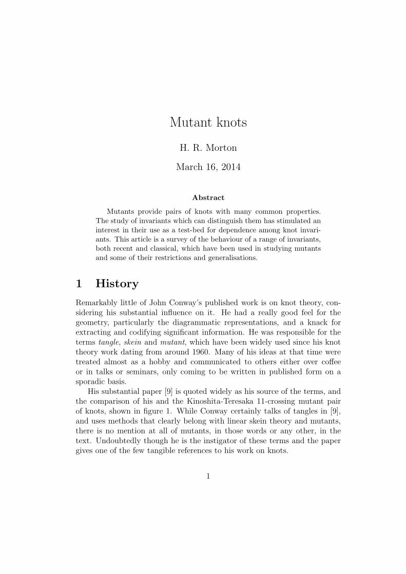
His substantial paper [9] is quoted widely as his source of the terms, andthe comparison of his and the Kinoshita-Teresaka 11-crossing mutant pairof knots, shown in figure 1. While Conway certainly talks of tangles in [9],and uses methods that clearly belong with linear skein theory and mutants,there is no mention at all of mutants, in those words or any other, in thetext. Undoubtedly though he is the instigator of these terms and the papergives one of the few tangible references to his work on knots.

1

In [9] Conway gives a table of 11 crossing knots, where he reckons to beconfident of differences among them, although without explicit invariants inall cases to be certain of this.

The two 11-crossing knots, C and KT , found by Conway and Kinoshita-Teresaka are probably the best-known example of inequivalent mutant knots.Conway’s knot is given in his table of 11-crossing knots [9], while KT appearsin [19] as one of a family of knots with trivial Alexander polynomial. Thesetwo knots are shown in figure 1.

C = KT =

Figure 1: The Conway and Kinoshita-Teresaka mutant pair

The first proof that the two knots in figure 1 are inequivalent was, Ibelieve, given by Riley [39].

Perko [37] tidied up the tables up to 11 crossings, and used double covertechniques in places to distinguish pairs of knots. These methods, however,would not be enough to distinguish a mutant pair, by theorem 3.

Gabai [15] used foliations in showing that C has genus 3 while KT hasgenus 2. The genus of a knot had until then been a difficult invariant todetermine exactly. Gabai’s work gave a much wider range of certainty, whilein principle the extension of the Alexander polynomial via Heegaard Floerhomology gives an exact calculation of the genus.

A recent systematic attempt to document mutant pairs among knots up to18 crossings has been undertaken by Stoimenow [42]. He also gives commentson the history and techniques available for distinguishing mutants, and thepractical limitations for calculations.

Disclaimer

While I have tried to find and credit historical work on mutants I have comeacross considerable difficulties in even identifying the initial sources of some

2

of the terms, such as Conway sphere. I have realised that much of the workhas been either in the realm of ‘folk-lore’, or implicit in places where theauthors have not felt it necessary to point up results arising from the generalmethods being discussed. Certainly one of the benefits of having to read olderpapers is the realisation of what can be deduced from an understanding ofthe ideas that underlie the work in question.

I would not want this article to be taken as providing a reliable historicalaccount, and I apologise for any omissions, both in material and in attribu-tion, that I suspect will be found in it.

2 Definitions

The most commonly used description of mutation is combinatorial, arisingdirectly from Conway’s definition of a tangle.

In his setting a tangle is a part of a knot diagram consisting of twoarcs contained in a circular region which meet the boundary circle in fourdiagonally placed points.

In line with current terminology I shall refer to this as a 2-tangle. Ingeneral a 2-tangle may contain closed curves as well as the two arcs, butsince in this article we will only be considering knots there will not be anyoccasion to look at 2-tangles with additional curves.

I shall also adjust the diagrams so that the containing region is a rectanglerather than a circle, with two boundary points of the arcs at the top and twoat the bottom.

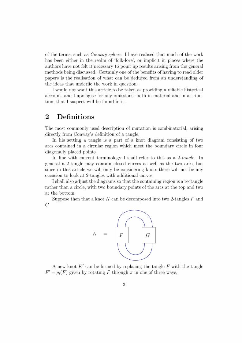
Suppose then that a knot K can be decomposed into two 2-tangles F andG

K = F G

A new knot K ′ can be formed by replacing the tangle F with the tangleF ′ = ρi(F ) given by rotating F through π in one of three ways,

3

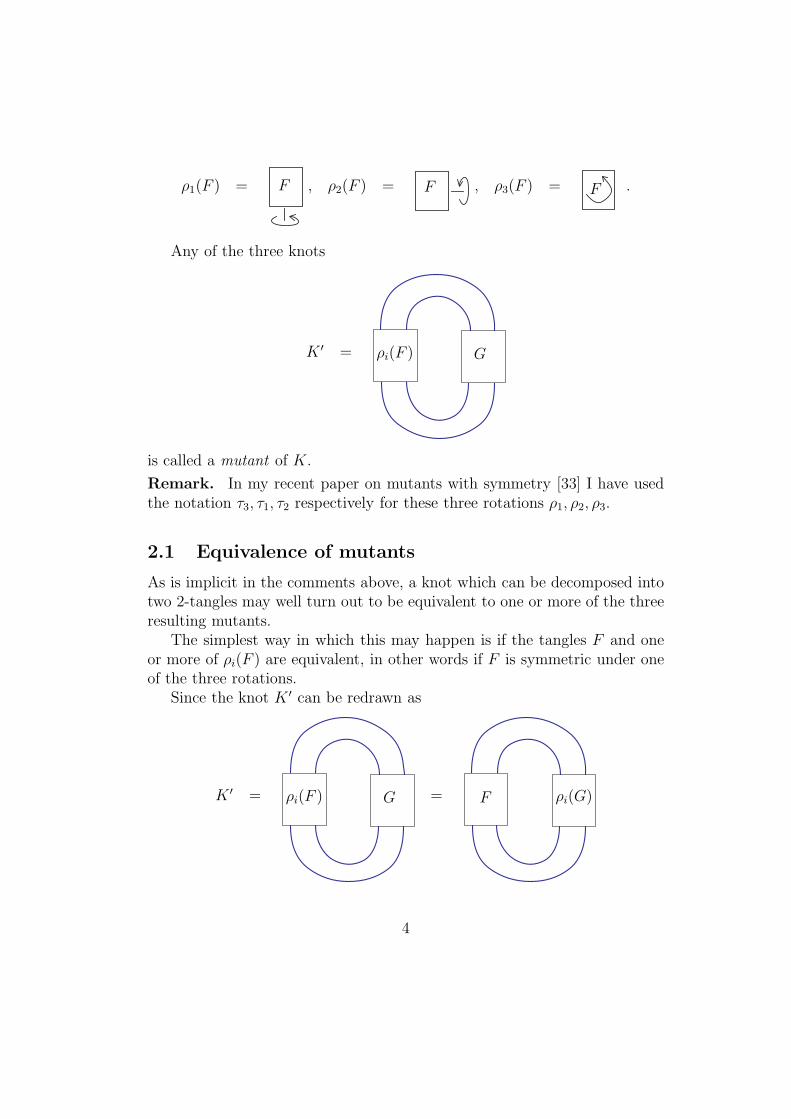
ρ1(F ) = F , ρ2(F ) = F , ρ3(F ) = F .

Any of the three knots

K ′ = ρi(F ) G

is called a mutant of K.

Remark. In my recent paper on mutants with symmetry [33] I have usedthe notation τ3, τ1, τ2 respectively for these three rotations ρ1, ρ2, ρ3.

2.1 Equivalence of mutants

As is implicit in the comments above, a knot which can be decomposed intotwo 2-tangles may well turn out to be equivalent to one or more of the threeresulting mutants.

The simplest way in which this may happen is if the tangles F and oneor more of ρi(F ) are equivalent, in other words if F is symmetric under oneof the three rotations.

Since the knot K ′ can be redrawn as

K ′ = ρi(F ) G = F ρi(G)

4

we will equally find that mutants are equivalent if the other tangle G hasrotational symmetry. Indeed, if F is symmetric under one of the rotationsand G is symmetric under a different rotation then all three mutants will beequivalent.

If one of the tangles has all three rotational symmetries then again allthe resulting mutants will be equivalent. This is of course the case when thetangle F consists simply of two non-crossing arcs. It is also true where F isa rational tangle, in Conway’s sense.

Rational tangles arise in Conway’s description from nicely arranged con-sequences of his notation where certain tangles appear in 1-1 correspondencewith rational numbers using a continued fraction decomposition.

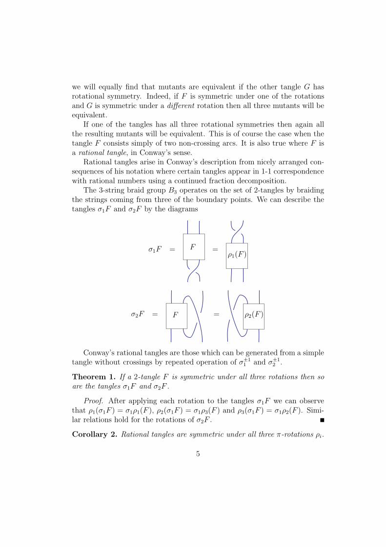
The 3-string braid group B3 operates on the set of 2-tangles by braidingthe strings coming from three of the boundary points. We can describe thetangles σ1F and σ2F by the diagrams

σ1F = F =ρ1(F )

σ2F = F = ρ2(F )

Conway’s rational tangles are those which can be generated from a simpletangle without crossings by repeated operation of σ±1

1 and σ±12 .

Theorem 1. If a 2-tangle F is symmetric under all three rotations then soare the tangles σ1F and σ2F .

Proof. After applying each rotation to the tangles σ1F we can observethat ρ1(σ1F ) = σ1ρ1(F ), ρ2(σ1F ) = σ1ρ3(F ) and ρ3(σ1F ) = σ1ρ2(F ). Simi-lar relations hold for the rotations of σ2F .

Corollary 2. Rational tangles are symmetric under all three π-rotations ρi.

5

Remark. Stoimenow makes use of this fact in his searches for mutant pairsamong knots up to 18 crossings [42], as he is able to exclude decompositionsin which one of the tangles is rational. By corollary 2 any mutation of sucha decomposition does not produce a different knot.

2.2 A three-dimensional view

There is a natural way of looking at mutants in a three-dimensional con-text, involving embedded 2-spheres in S3 meeting a knot transversely in fourpoints. Ruberman [41] adopted the current term Conway sphere for such anembedded sphere.

The two 3-balls which lie on either side of a Conway sphere then corre-spond to a decomposition of the knot into two 2-tangles, although there willbe a choice involved in representing each of these by a diagram. In effect thediagram will be determined up to the action of the braid group B3 on thepunctures on the sphere.

If the knot in S3 is regarded as an orbifold with cone angle π along theknot then the Conway spheres play a natural role in the theory of orbifolddecompositions, which is mirrored by their torus covers in the 2-fold cycliccover of S3 branched over the knot. Bonahon and Siebenmann [6] provea uniqueness result for orbifold decompositions in a general setting, Theirresults apply in this case with suitable Conway spheres providing the coun-terpart to the tori in the Jaco-Shalen decomposition of the covering manifold.

The following result is noted by Viro [44], who uses the term twin ratherthan mutant.

Theorem 3. The double covers of S3 branched over mutant knots are home-omorphic.

Proof. The double cover of a knot and its mutant by ρi are constructedfrom the double covers of the two constituent tangles by gluing along thetorus covering the Conway sphere. The two double covers then differ by thehomeomorphism of the torus which covers ρi. For each i this homeomorphismis isotopic to the identity.

In his paper analysing the behaviour of Conway spheres in knots Lickorish[23] uses the term untangled to denote a tangle which is homeomorphic to thetrivial tangle, that is, where there is a homeomorphism of the 3-ball carryingthe two arcs inside the Conway sphere to a pair of parallel unknotted arcs.

6

Such tangles are exactly the rational tangles of Conway. (Viro notes that anyπ-rotated untangled tangle is isotopic to the original tangle by an isotopywhich fixes the boundary sphere.)

It is then easy to give a quick proof of the following result (see also theproof of Rolfsen [40]).

Theorem 4. The only mutant of the unknot is the unknot.

Proof. Suppose that we have a Conway sphere meeting the unknot infour points. The fundamental group of the four-punctured sphere is free on3 generators. This cannot inject into both fundamental groups of the tangleson the two sides, otherwise it would inject into the fundamental group ofthe knot complement. Hence, by Dehn’s lemma, there is a non-trivial closedcurve on the Conway sphere which bounds a disc disjoint from the arcs inone of the tangles. This disc must separate the two arcs in the ball. Eacharc must be unknotted, as it is then a connected summand of the unknot.Hence this tangle is untangled in the sense of Lickorish. It is then a rationaltangle and is symmetric under all three rotations, and so the mutants are allequivalent.

We have seen here that certain tangle decompositions will only give riseto equivalent mutants. When analysing a tangle decomposition a first checkshould then be made on the possible symmetries of the constituent tangles.On the other hand, when we suspect that two mutants may not be equivalent,there remains the question of showing that they are indeed different.

In the next section I shall give a selection of classical methods, bothgeometric and algebraic, which have been been used to distinguish betweenmutant pairs, and some early limitations which were noted. In the followingsections I shall give some of the known invariants which all mutants mustshare, and further conditions under which a greater range of invariants areshared. In this way the use of mutants contributes a means of looking atpossible relations between new and existing invariants, in terms of the extentto which they may agree on various classes of mutants.

3 Classical ways to distinguish mutants

Here the term ‘classical’ refers to techniques that were in use up to thediscovery of the Jones polynomial in 1984. I have loosely separated themethods used under the general headings of algebraic and geometric.

7

3.1 Algebraic

The simplest method of distinguishing knots is by means of the Alexanderpolynomial, which can be calculated readily from a Seifert matrix for theknot.

Viro [44] uses comparable Seifert matrices for mutant knots to observethat their Alexander polynomials are the same, along with the homologygroups and forms of linking coefficients in branched covers, Minkowski unitsand signatures, all of which can be found from a Seifert matrix. The Seifertmatrices constructed by Viro are either identical or have the form

S =

A C 0CT a DT

0 D B

, S ′ =

A C 0CT a DT

0 D BT

,

where A and B are square matrices, C and D are column matrices.Viro proves that the Whitehead doubles of the connected sums K#K

and K#Kr are inequivalent mutants when K is a knot which is inequivalentto its reverse Kr. This follows since equivalence of the Whitehead doublesimplies equivalence of the connected sums, and decomposition of connectedsums is unique.

He notes also that the whole series of knots with trivial Alexander poly-nomial described by Kinoshita and Teresaka in [19] all have obvious mutantsalthough he does not give a systematic way of ensuring that all of these pairsare inequivalent.

In the absence of information from the Alexander polynomial, the mostbasic algebraic way to show that two knots are inequivalent is to comparemore directly their groups, in other words the fundamental groups of theircomplements.

Apart from questions of mirror images and orientation, two inequivalentmutants will have non-isomorphic groups, by the general results of Gordonand Luecke. There is then a good chance of detecting a difference by com-paring homomorphisms of their groups into suitable finite groups.

Early distinctions among knots were made by this method by Riley [39],who separated the Conway and Kinoshita-Teresaka 11-crossing knots bymeans of homomorphisms from the knot group to PSL(2, 7). Riley treatsthis group as a subgroup of the symmetric group S7, and considers repre-sentations in which meridians are mapped to 7-cycles. Calculation of thehomology groups of the resulting 7-fold coverings branched over the knotdemonstrates a difference between the two knots.

8

The use of homomorphisms of knot groups to finite groups is knowngenerally as knot colouring. These methods include the classical 3-colouringand n-colouring, where the finite group used is the dihedral group Dn. Thesetechniques were much used in their original form by Fox, who extended themethods in [14]. The techniques are essentially those developed, notably byFenn and Rourke [13], under the current term of quandle. It is immediatethat n-colouring will not distinguish mutant pairs, since the existence of an n-colouring depends on the Alexander polynomial, and Alexander polynomialsare shared by mutants.

3.2 Geometric

Geometric methods available for distinguishing knots include comparison ofrelated 3-dimensional manifolds covering S3 and branched over the knot indifferent ways.

3.2.1 Covers

The simplest of such constructions is the double cover. Viro gives a nicesummary of the behaviour of mutants, referred to as twins in [44]. He provesin Theorem 3 that the double covers of S3 branched over two mutant knotsare homeomorphic. So something more elaborate is needed to distinguishmutants by this type of argument.

More complicated covers can be related to homomorphisms from the knotgroup to a finite group, as in Riley’s arguments in [39], which proved to beeffective in distinguishing between the 11-crossing knots C and KT .

3.2.2 Genus

An early geometric invariant of a knot is its genus, which is the least genusamong orientable surfaces spanning the knot in S3. The simplicity of itsdefinition has made it a popular invariant, but it is not easy to calculatein general. It can be bounded below in terms of the Alexander polynomial,but in many cases this bound is not exact. Since the Alexander polynomialagrees on mutants this bound will not be helpful in distinguishing mutants.

It is a surprise that the genus of mutants can differ. Gabai developedtechniques for calculating the genus, based on the use of foliations, which

9

gave an early distinction between C and KT . He showed in [15] that C hasgenus 3 while KT has genus 2.

It is only much more recently that the Heegaard-Floer homology of a knothas provided an exact calculation of the genus in all cases.

3.2.3 Diagrammatic invariants

Although the genus can be different for mutants, it is not known whetherinvariants such as the crossing number, the braid index or the arc index, canever differ on mutants.

The best hope for settling any of these questions would be to give adirect argument that mutants must have the same braid index (defined asthe least number n of strings needed to present the knot as a closed n-braid).Attempts to show that two mutants have different braid index run up againstthe difficulty that one of the best ways to find a lower bound for the braidindex relies on the use of knot polynomials and many of these are shared bymutants.

3.2.4 Hyperbolic geometry

Bonahon and Siebenmann, along with others from Orsay, analysed the struc-ture of classes of knots with the goal of extending and systematising Conway’sconstructions. Their original work was contained in an influential series ofnotes, which never itself formed a complete publication, although much isavailable in their ongoing draft monograph [7]. In the course of their workthey made much use of Conway sphere-based decompositions. This culmi-nated in an extensive analysis of knots from the point of view of orbifolds,where the knot formed a subset with cone angle π. These early geometricobservations for knots were used in [6] to formulate an orbifold decompositiontheorem which is a counterpart to the Jaco-Shalen-Johannson decompositionfor 3-manifolds.

Recent work on this, and related bibliographies can be found in work ofBoileau et al [5] and Paoluzzi [36], for example.

With the advent of Thurston’s work on hyperbolic and other geomet-ric structures on 3-manfolds there followed a more systematic view of knotcomplements from a geometric point of view.

In particular the default position for a knot complement in the absenceof certain special features turns out to be that there is a complete hyperbolic

10

structure of finite volume on the complement. The volume is an invariant ofthe knot. However Ruberman [41] shows that if a knot K is hyperbolic, thenany mutant is also hyperbolic, and they have the same hyperbolic volume.

Weeks [45] developed the amazingly powerful program SnapPea to calcu-late details of hyperbolic manifolds, including the volume and other detailsmaking up an invariant ‘canonical structure’. While the volume on its ownis not enough, it is possible to use the canonical structures to distinguishinequivalent mutants.

3.2.5 Symmetry

In the same paper [41] Ruberman remarks that the work of Bonahon andSiebenmann [6, 7] ensures that if two mutant knots are equivalent then theremust be some rotational symmetries in the constituent 2-tangles. In princi-ple then mutants can be distinguished by showing that the tangles have nosuitable symmetry. Subsequently Ruberman and Cochran [8] were able tofind a means of ruling out symmetry in some tangles, and apply it to giveexamples of inequivalent mutants.

4 Polynomials and quantum invariants

The enormous range of invariants which followed the discovery of the Jonespolynomial and its generalisations from 1984 onwards has made availablemany further theoretical and practical ways of comparing knots. Besidesusing the new invariants to compare mutants it has also proved fruitful toregard mutants and their refinements as a tool for analysing possible depen-dence among invariants.

Very shortly after the discovery of the new invariants Lickorish proved,using simple skein theoretic arguments, that mutants must also have identicalHomfly and Kauffman polynomials, and hence the same Jones polynomial.A good account of this can be found in his survey article [24].

Calculations of Morton and Short for a number of examples led to theconjecture [31] that two equally twisted 2-cables of a mutant pair would alsoshare the same Homfly polynomial. This was proved by Lickorish and Lipson[25], also using skein theory. They showed further that the same result holdsfor reverse-string 2-cables (that is, for 2-cables of two components whoseorientations run in opposite directions, giving a ‘reverse parallel’ satellite).

11

This holds equivalently for equally twisted Whitehead doubles. These resultswere also derived independently by Przytycki [38].

Although the Homfly polynomials of doubles or 2-cables were found not todistinguish mutants it was already clear that invariants of more complicatedsatellites of knots could provide extra information in general.

4.1 Homfly invariants

In 1984 V.F.R.Jones constructed a new invariant of oriented links VL(t) ∈Z[t±

1

2 ], which turned out to have the property that

t−1VL+− tVL−

= (√

t − 1/√

t)VL0(1)

for links L± and L0 related as in the Conway polynomial relation. This wasquickly extended to a 2-variable invariant PL(v, z) ∈ Z[v±1, z±1], with theproperty that

v−1PL+− vPL−

= zPL0. (2)

The name ‘Homfly polynomial’ has come to be attached to P , beingthe initial letters of six of the eight people involved in this further devel-opment. The name is sometimes extended to the more unwieldy ‘HOM-FLYPT’, to make reference to all eight. The polynomial P contains both theConway/Alexander polynomial, and Jones’ invariant, and can be shown tocontain more information in general than both of these taken together. Itsatisfies the equations

P (1, z) = ∇(z)

P (1, s − s−1) = ∆(s2)

P (s2, s − s−1) = V (s2)

P (s, s − s−1) = ±1

The skein relation (2) can readily be shown to determine P and V once itsvalue on the trivial knot is given. It has been usual to take P = 1 on thetrivial knot, although in some recent applications a different normalisationcan be more appropriate.

Given the existence of V and P we can then make some calculations. Forexample, the unlink with two components has

P =v−1 − v

z,

V (s2) = −(s + s−1),

12

while the Hopf link with linking number +1 has

P = vz + (v−1 − v)v2z−1,

V (s2) = s3 − s − (s + s−1)s4 = −s(1 + s4).

The Hopf link with linking number −1 has

P = −v−1z + (v−1 − v)v−2z−1,

V (s2) = −s−1(1 + s−4).

This illustrates the general feature that for the mirror image L of a link L,(where the signs of all crossings are changed), we have PL(v, z) = PL(v−1,−z)and so VL(s2) = VL(s−2). It is thus quite possible to use V in many cases todistinguish a knot from its mirror-image, while there will be no difference intheir Conway polynomials. It is worth noting that although there are stillknots which cannot be distinguished from each other by P in spite of beinginequivalent, no non-trivial knot has so far been found for which P = 1, oreven V = 1.

4.1.1 Framed versions

The original Homfly polynomial is invariant under all Reidemeister moves,but there is a convenient version which is an invariant of a framed orientedlink. A more extended discussion of the exact choice of framing normalisa-tions can be found elsewhere, [2, 27, 26].

In its most adaptable form, PL(v, s), the framed invariant lies in the ring

Λ = Z[v±1, s±1, (sr − s−r)−1], r > 0.

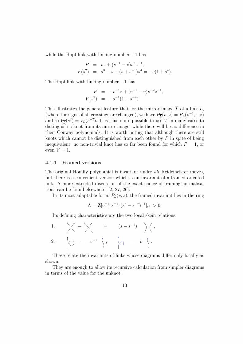
Its defining characteristics are the two local skein relations.

1. − = (s − s−1) ,

2. = v−1 , = v .

These relate the invariants of links whose diagrams differ only locally asshown.

They are enough to allow its recursive calculation from simpler diagramsin terms of the value for the unknot.

13

4.2 Satellite invariants

Invariants such as the Homfly polynomial P of any choice of satellite of aknot K may be regarded as invariants of K itself. These provide a wholerange of satellite invariants, which can be compared for mutants K and K ′.

4.2.1 Framed links

Framed links are made from pieces of ribbon rather than rope, so that eachcomponent has a preferred annulus neighbourhood.

Combinatorially they can be modelled by diagrams in S2 up to the Reide-meister moves RII and RIII , excluding RI , by use of the ‘blackboard framing’convention. The ribbons are determined by taking parallel curves on the di-agram. Reidemeister moves RII and RIII on a diagram give rise to isotopicribbons. Any apparent twists in a ribbon can be flattened out using RI .

Oriented link diagrams D have a writhe w(D) which is the sum of thesigns of all crossings. This is unchanged by moves RII and RIII .

The unframed version of the Homfly polynomial for an oriented link L,invariant under all Reidemeister moves, is given from this framed version byvw(D)PL(v, s) where D is a diagram for the framed link.

Remark. For a framed knot the writhe is sometimes called its ‘self-linkingnumber’, which is independent of the orientation of the diagram. Generallya framing of a link is determined by a choice of writhe for each component.

4.2.2 Satellites

A satellite of a framed knot K is determined by choosing a diagram Q in thestandard annulus, and then drawing Q on the annular neighbourhood of Kdetermined by the framing, to give the satellite knot K ∗Q. We refer to thisconstruction as decorating K with the pattern Q (see figure 2).

Morton and Traczyk [32] showed that the Jones polynomial V cannot beused in combination with any choice of satellite to distinguish a mutant pair,K and K ′. Thus VK∗Q = VK ′∗Q for any choice of pattern Q, provided thatthe same framing of K and K ′ is used.

4.2.3 A parameter space for Homfly satellite invariants

The local nature of the Homfly skein relations allows us to make a usefulsimplification in studying Homfly satellite invariants PK∗Q as the pattern Q

14

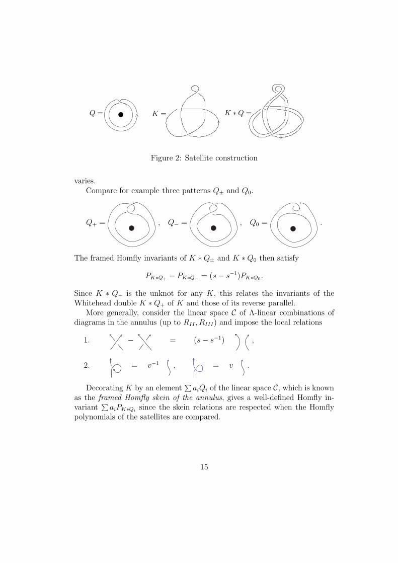
Q = K = K ∗ Q =

Figure 2: Satellite construction

varies.Compare for example three patterns Q± and Q0.

Q+ = , Q− = , Q0 = .

The framed Homfly invariants of K ∗ Q± and K ∗ Q0 then satisfy

PK∗Q+− PK∗Q−

= (s − s−1)PK∗Q0.

Since K ∗ Q− is the unknot for any K, this relates the invariants of theWhitehead double K ∗ Q+ of K and those of its reverse parallel.

More generally, consider the linear space C of Λ-linear combinations ofdiagrams in the annulus (up to RII , RIII) and impose the local relations

1. − = (s − s−1) ,

2. = v−1 , = v .

Decorating K by an element∑

aiQi of the linear space C, which is knownas the framed Homfly skein of the annulus, gives a well-defined Homfly in-variant

∑

aiPK∗Qisince the skein relations are respected when the Homfly

polynomials of the satellites are compared.

15

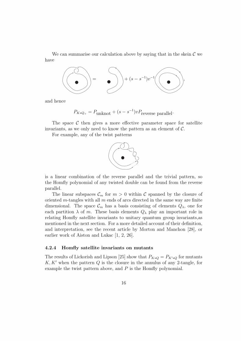
We can summarise our calculation above by saying that in the skein C wehave

= + (s − s−1)v−1 ,

and hence

PK∗Q+= Punknot + (s − s−1)vPreverse parallel.

The space C then gives a more effective parameter space for satelliteinvariants, as we only need to know the pattern as an element of C.

For example, any of the twist patterns

is a linear combination of the reverse parallel and the trivial pattern, sothe Homfly polynomial of any twisted double can be found from the reverseparallel.

The linear subspaces Cm for m > 0 within C spanned by the closure oforiented m-tangles with all m ends of arcs directed in the same way are finitedimensional. The space Cm has a basis consisting of elements Qλ, one foreach partition λ of m. These basis elements Qλ play an important role inrelating Homfly satellite invariants to unitary quantum group invariants,asmentioned in the next section. For a more detailed account of their definition,and interpretation, see the recent article by Morton and Manchon [28], orearlier work of Aiston and Lukac [1, 2, 26].

4.2.4 Homfly satellite invariants on mutants

The results of Lickorish and Lipson [25] show that PK∗Q = PK ′∗Q for mutantsK, K ′ when the pattern Q is the closure in the annulus of any 2-tangle, forexample the twist pattern above, and P is the Homfly polynomial.

16

A contrasting result occurs when the pattern Q is a closed 3-tangle. Hom-fly invariants of 3-parallels were realised at an early stage to give possibilitiesfor distinguishing mutants.

Calculations made in 1986 by Morton and Traczyk showed that the Hom-fly polynomials PC∗Q and PKT∗Q are different for the 3-parallel pattern Q.Since the computing facilities available were limited they fixed the value ofone variable and reduced the integer coefficients mod p for some small fixedvalue of p. Although they were able to establish that the two polynomialswere different it was not easy to appreciate the extent and nature of thedifference from their calculations. Jun Murakami [34] also made calculationsbased on 3-parallels of other mutant pairs, and gave necessary conditionsfor Homfly-based satellite invariants to distinguish mutants. These involveidentification of dimension 1 subspaces in representation theory.

Subsequent more sophisticated calculations by Cromwell and Morton [27]give much more detail. Their method of calculation involves a truncationwhich amounts to retaining only Vassiliev invariants up to a certain type,in this case type 12 is enough. Such a truncation at a fixed type is veryeasily implemented in terms of the calculations based on the Morton-Shortalgorithm for finding Homfly polynomials [31], and it gives a very satisfactoryoutcome when the difference of the invariants for two mutants is studied.

4.2.5 Kauffman polynomial

The 2-variable Kauffman polynomial, discovered shortly after the appearanceof the Homfly polynomial, also has the property that it does not distinguishmutants. Nor does it distinguish the 2-parallels of mutants.

Rather less work has been done on establishing which Kauffman satelliteinvariants can distinguish mutants. Like the Homfly polynomial its satelliteinvariants are closely related to quantum group invariants [46]. More recentcalculations have been made by Stoimenow [42] who has shown that theKauffman polynomial of the 3-parallel can distinguish some mutants withsymmetry, in contrast to the corresponding Homfly polynomial.

5 Unitary quantum group invariants

Following closely after the discovery of the Homfly and Kauffman polynomialinvariants came the work of Reshetikhin and Turaev on the development of

17

knot invariants based on quantum groups.Quantum groups give rise to 1-parameter invariants J(K; W ) of an ori-

ented framed knot K depending on a choice of finite dimensional moduleW over the quantum group, following constructions of Turaev and others[43, 46]. This choice is referred to as colouring K by W , and can be ex-tended for a link to allow a choice of colour for each component.

5.1 Basic constructions of quantum invariants

A quantum group G is an algebra over a formal power series ring Q[[h]],typically a deformed version of a classical Lie algebra. A finite dimensionalmodule over G is a linear space on which G acts.

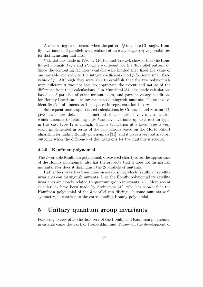
Crucially, G has a coproduct ∆ which ensures that the tensor productV ⊗ W of two modules is also a module. It also has a universal R-matrix (ina completion of G⊗G) which determines a well-behaved module isomorphism

RV W : V ⊗ W → W ⊗ V.

This has a diagrammatic view indicating its use in converting colouredtangles to module homomorphisms.

W ⊗ V

V ⊗ W

RV W

A braid β on m strings with permutation π ∈ Sm and a colouring of thestrings by modules V1, . . . , Vm leads to a module homomorphism

Jβ : V1 ⊗ · · · ⊗ Vm → Vπ(1) ⊗ · · · ⊗ Vπ(m)

using R±1Vi,Vj

at each elementary braid crossing. The homomorphism Jβ de-pends only on the braid β itself, not its decomposition into crossings, by theYang-Baxter relation for the universal R-matrix.

When Vi = V for all i we get a module homomorphism Jβ : W →W , where W = V ⊗m. Now any module W decomposes as a direct sum⊕

(Wµ ⊗ V (N)µ ), where Wµ ⊂ W is a linear subspace consisting of the highest

weight vectors of type µ associated to the module V (N)µ . Highest weight

subspaces of each type are preserved by module homomorphisms, and so Jβ

determines (and is determined by) the restrictions Jβ(µ) : Wµ → Wµ for eachµ, where µ runs over partitions with at most N parts.

18

If a knot (or one component of a link) K is decorated by a pattern T whichis the closure of an m-braid β, then its quantum invariant J(K ∗ T ; V ) canbe found from the endomorphism Jβ of W = V ⊗m in terms of the quantuminvariants of K and the restriction maps Jβ(µ) : Wµ → Wµ by the formula

J(K ∗ T ; V ) =∑

cµJ(K; V (N)µ ) (3)

with cµ = trJβ(µ). This formula follows from lemma II.4.4 in [43]. We setcµ = 0 when W has no highest weight vectors of type µ.

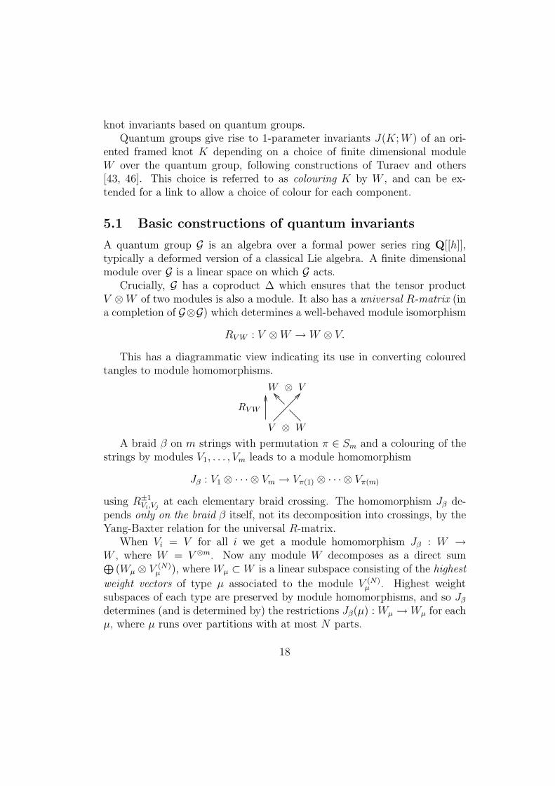
More generally the methods of Reshetikhin and Turaev allow the quantumgroups G = sl(N)q to be used to represent oriented tangles whose componentsare coloured by G-modules as G-module homomorphisms. One additionalfeature is needed, namely the use of the dual module V ∗ defined by means ofthe antipode in G, (an antiautomorphism of G which is part of its structureas a Hopf algebra). When the components of the tangle are coloured bymodules the tangle itself is represented by a homomorphism from the tensorproduct of the modules which colour the strings at the bottom to the tensorproduct of the modules which colour the strings at the top, provided thatthe string orientations are inwards at the bottom and outwards at the top.The dual module V ∗ comes into play in place of V when an arc of the tanglecoloured by V has an output at the bottom or an input at the top.

For example, the (4, 2)-tangle below, when coloured as shown, is repre-sented by a homomorphism U ⊗ W ∗ → U ⊗ X∗ ⊗ X ⊗ W ∗.

U

V W

X

U X* X W*

U W*

It is possible to build up the definition so that consistently coloured tanglesare represented by the appropriate composite homomorphisms, starting froma definition of the homomorphisms for the elementary oriented tangles. Twocases, depending on the orientation, must be considered for both the local

19

maximum and the local minimum, and a little care is needed here to ensureconsistency. The final result is a definition of a homomorphism which isinvariant when the coloured tangle is altered by RII and RIII . When appliedto an oriented k-component link diagram L regarded as an oriented (0, 0)-tangle it gives an element J(L; V1, . . . , Vk) ∈ Λ = Q[[h]] for each colouringof the components of L by G-modules, which is an invariant of the framedoriented link L.

The construction is simplified in the case of sl(2)q by the fact that allmodules are isomorphic to their dual, and so orientation of the strings playsno role.

5.2 Quantum invariants of mutant knots

We turn to the question of distinguishing mutants such as C and KT bymeans of quantum group invariants, especially those which use the unitaryquantum groups sl(N)q. These are closely related to the Homfly satelliteinvariants of a knot, and can provide complementary insights into their be-haviour.

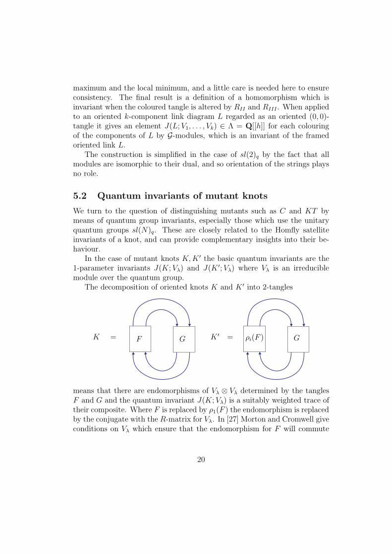
In the case of mutant knots K, K ′ the basic quantum invariants are the1-parameter invariants J(K; Vλ) and J(K ′; Vλ) where Vλ is an irreduciblemodule over the quantum group.

The decomposition of oriented knots K and K ′ into 2-tangles

K = F G K ′ = ρi(F ) G

means that there are endomorphisms of Vλ ⊗ Vλ determined by the tanglesF and G and the quantum invariant J(K; Vλ) is a suitably weighted trace oftheir composite. Where F is replaced by ρ1(F ) the endomorphism is replacedby the conjugate with the R-matrix for Vλ. In [27] Morton and Cromwell giveconditions on Vλ which ensure that the endomorphism for F will commute

20

with the R-matrix, so that J(K; Vλ) = J(K ′; Vλ), when K ′ is the mutantconstructed using the rotation ρ1.

Remark. This is the case known as the positive mutant in 8.2.1. They alsogive conditions which ensure equality for quantum invariants of the othermutants.

5.3 Unitary quantum invariants and Homfly invariants

When dealing with sl(N)q for any fixed natural number N it is usual to writeq = eh. Where the framed knot K is coloured by a finite dimensional moduleW over the unitary quantum group sl(N)q its invariant J(K; W ) depends onthe variable h as a Laurent polynomial in one variable s = eh/2 =

√q, up to

an overall fractional power of q.The invariant J is linear under direct sums of modules and all the modules

over sl(N)q are semi-simple, so we can restrict our attention to the irreducible

modules V(N)λ . For sl(N)q these are indexed by partitions λ with at most

N parts, without distinguishing two partitions which differ in some initialcolumns with N cells each.

There is a close relation between Homfly satellite invariants and unitaryquantum invariants of K. To help in our comparison of these invariants wewrite P (K; Q) for PK∗Q and more generally

P (L; Q1, Q2, . . . , Qk)

for the Homfly polynomial of a link L when its components are decorated byQ1, . . . , Qk respectively.

Theorem 5 (Comparison theorem).

1. The sl(N)q invariant for the irreducible module V(N)λ is the Homfly in-

variant for the knot decorated by Qλ with v = s−N , suitably normalisedas in [26]. Explicitly,

P (K; Qλ)|v=s−N = xk|λ|2J(K; V(N)λ )

where k is the writhe of K, and x = s1/N .

2. Each invariant P (K; Q)|v=s−N is a linear combination of quantum in-variants

∑

cαJ(K; Wα).

21

3. Each J(K; W ) is a linear combination of Homfly invariants

∑

djP (K; Qj)|v=s−N .

Remark.

• In the special case when N = 2 we can interpret quantum invariantsof K in terms of Kauffman bracket satellite invariants, using the skeinof the annulus based on the Kauffman bracket relations. This sim-pler skein is a quotient of the algebra C. More generally the sl(N)q

invariants depend only on a quotient of the algebra C for each N .

• The quantum group invariants based on sl(3)q also admit a combina-torial simplification due to Kuperberg to allow an easier diagrammaticcalculation of them. At the same time the quantum group itself isstraightforward enough to make it possible to work directly with someof the smaller dimensional modules, [29, 33].

• The 2-variable invariant P (K; Q) can be recovered from the specialisa-tions P (K; Q)|v=s−N for sufficiently many N .

• If the pattern Q is a closed braid on m strings then we only need usepartitions λ ⊢ m, since Cm is spanned by {Qλ}λ⊢m. Conversely, to

realise J(K; V(N)λ ) with λ ⊢ m we can use closed m-braid patterns.

The basic condition on the quantum group module Vλ in [27] is that whenthe module Vλ ⊗ Vλ is decomposed as a direct sum of irreducible modulesthere should be no repeated summands, up to isomorphism. In this case anytwo endomorphisms of Vλ ⊗ Vλ will commute.

Since this is the case for all irreducible sl(2)q modules Vλ, it gives an al-ternative proof of the results of Morton-Traczyk about the Jones polynomialof satellites of mutants.

It is also the case for the fundamental irreducible sl(N)q module withYoung diagram , which, taken together for all N , determine the Homflypolynomial, and for the irreducible sl(N)q modules with Young diagramsand , which determine the Homfly polynomial of the directed 2-cables.

It is interesting that this condition does not establish Lickorish and Lip-son’s result that the Homfly polynomial of reverse 2-parallels must agree for

22

mutants; their result then yields a non-trivial consequence for quantum in-variants. The simplest example of this is that the sl(3)q invariant of a knotwhen coloured by the irreducible module with Young diagram will agree

on a mutant pair. I suspect that this invariant is at the heart of Stoimenow’suse of the Whitehead double in showing that a pair of knots are not mutants[42]. He gives a pair of knots whose Homfly polynomials of their 2-parallels,and of the knots themselves, agree, and proves that the knots are not mutantsbecause the Homfly polynomials of their Whitehead doubles are different.

The calculations of Cromwell and Morton [27] about the Homfly polyno-mials of 3-parallels show, on the other hand, that the sl(4)q invariant for themodule with Young diagram does distinguish some mutant pair, namely

C and KT , as does the sl(N)q invariant with Young diagram , for every

N ≥ 4.

6 Vassiliev invariants

The invariants, known variously as finite type invariants or Vassiliev invari-ants, developed by Vassiliev and Gusarov in the late 80s, can be relatedreadily to polynomial and quantum group invariants, originally by Birmanand Lin [3]. They provide a rather transverse view of a whole collectionof these invariants, and their behaviour on mutants has been a matter ofcontinuing interest.

Chmutov, Duzhin and Lando [12] prove that all Vassiliev invariants ofdegree at most 8 agree on any mutant pair of knots.

This is extended to Vassiliev invariants up to degree 10 by Jun Murakami[35], where he also confirms the degree 11 invariant used by Morton andCromwell in [27] which can be used to distinguish the knots C and KT .

Morton and Cromwell expand the difference between the Homfly polyno-mials of the 3-parallels of the knots C and KT to isolate a framed Vassilievinvariant of type 11 which distinguishes these two mutants, and go on to ex-plain some features of the difference PK∗Q − PK ′∗Q for general K, K ′, wherethe pattern Q is the closure of a 3-braid.

Further results about Vassiliev invariants on extended and restrictedclasses of mutants are noted in section 8.

23

7 Further invariants

Among the homology invariants which have been developed in the past 10years the Heegaard-Floer homology can certainly distinguish some mutants,since it is able to calculate the genus of the knot.

On the other hand Bloom [4] shows that odd Khovanov homology forknots is unchanged by mutation. As a corollary he notes that Khovanovhomology over Z2 is also mutation invariant. Homfly Khovanov homology isshown by Jaeger [17] to be invariant under positive mutation, as defined in8.2.1.

Kim and Livingston [20] show that the 4-ball genus of a knot can bechanged by mutation, but the algebraic concordance class is invariant undermutation.

7.1 Behaviour on mutants

I have gathered together here a summary of the results noted about the be-haviour of a selection of invariants on mutants. Where the invariants areknown to be the same on mutant knots (shared) I give a reference to a proof,not necessarily the original one. Where there are mutants on which the in-variant is known to differ I give a reference to an example.

24

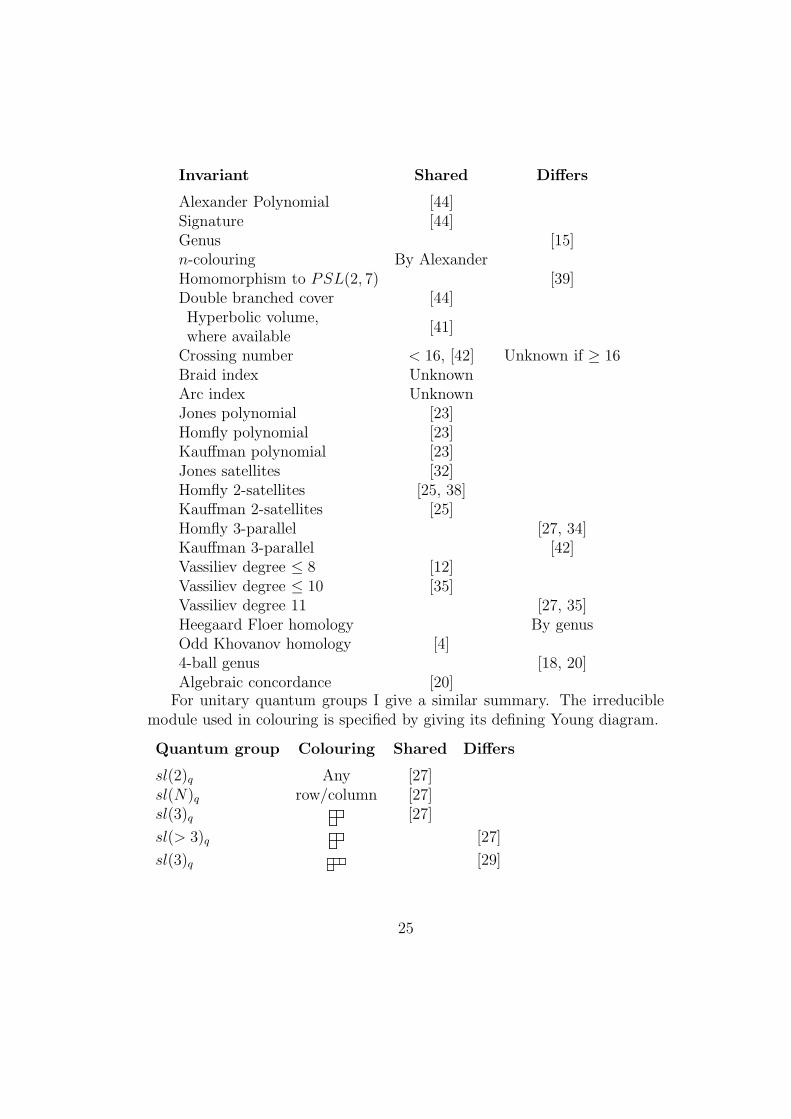
Invariant Shared Differs

Alexander Polynomial [44]Signature [44]Genus [15]n-colouring By AlexanderHomomorphism to PSL(2, 7) [39]Double branched cover [44]Hyperbolic volume,where available

[41]

Crossing number < 16, [42] Unknown if ≥ 16Braid index UnknownArc index UnknownJones polynomial [23]Homfly polynomial [23]Kauffman polynomial [23]Jones satellites [32]Homfly 2-satellites [25, 38]Kauffman 2-satellites [25]Homfly 3-parallel [27, 34]Kauffman 3-parallel [42]Vassiliev degree ≤ 8 [12]Vassiliev degree ≤ 10 [35]Vassiliev degree 11 [27, 35]Heegaard Floer homology By genusOdd Khovanov homology [4]4-ball genus [18, 20]Algebraic concordance [20]

For unitary quantum groups I give a similar summary. The irreduciblemodule used in colouring is specified by giving its defining Young diagram.

Quantum group Colouring Shared Differs

sl(2)q Any [27]sl(N)q row/column [27]sl(3)q [27]

sl(> 3)q [27]

sl(3)q [29]

25

8 Generalisations and restrictions

8.1 Generalisations

Various generalisations of the original ideas of mutants have been made.

8.1.1 Rotors

An obvious possibility is to decompose a knot by a sphere meeting the knotin 2n points with n > 2, and then replace one side of the sphere after sometransformation. In many cases the resulting knot does not have enoughproperties in common with the original for this to be worthwhile. HoweverRolfsen [40] has used the idea of a rotor, based on 2n intersection pointsaround the equator of a sphere with a rotation of order 2n on one side asthe transformation. For unoriented knot diagrams this operation preservesthe Jones polynomial, although Rolfsen has so far not been able to use themethod in his searches for a non-trivial knot with Jones polynomial V = 1.

8.1.2 Genus 2 mutants

A more fruitful class of generalised mutants are constructed by finding anembedded genus 2 surface in the knot complement, and regluing the twosides after a suitable degree 2 transformation (a hyperelliptic involution).This construction was used by Ruberman [41] for general 3-manifolds, andby Cooper and Lickorish [10] in the context of knots in S3.

The construction has a close relation to Conway mutation for knots, whichcan be realised by applying a sequence of one or two genus 2 mutations. Anextensive discussion of genus 2 mutation, and properties which are known tobe preserved, is given by Dunfield et al [11]. Further calculations related togenus 2 mutants by Morton and Nathan Ryder appear in [30].

Here are some of the known coincidences and differences.

26

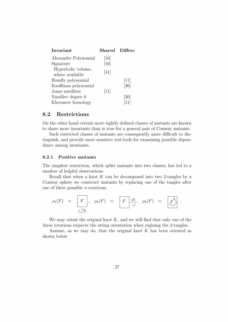
Invariant Shared Differs

Alexander Polynomial [10]Signature [10]Hyperbolic volume,where available

[41]

Homfly polynomial [11]Kauffman polynomial [30]Jones satellites [11]Vassiliev degree 8 [30]Khovanov homology [11]

8.2 Restrictions

On the other hand certain more tightly defined classes of mutants are knownto share more invariants than is true for a general pair of Conway mutants.

Such restricted classes of mutants are consequently more difficult to dis-tinguish, and provide more sensitive test-beds for examining possible depen-dence among invariants.

8.2.1 Positive mutants

The simplest restriction, which splits mutants into two classes, has led to anumber of helpful observations.

Recall that when a knot K can be decomposed into two 2-tangles by aConway sphere we construct mutants by replacing one of the tangles afterone of three possible π-rotations.

ρ1(F ) = F , ρ2(F ) = F , ρ3(F ) = F .

We may orient the original knot K, and we will find that only one of thethree rotations respects the string orientation when regluing the 2-tangles.

Assume, as we may do, that the original knot K has been oriented asshown below

27

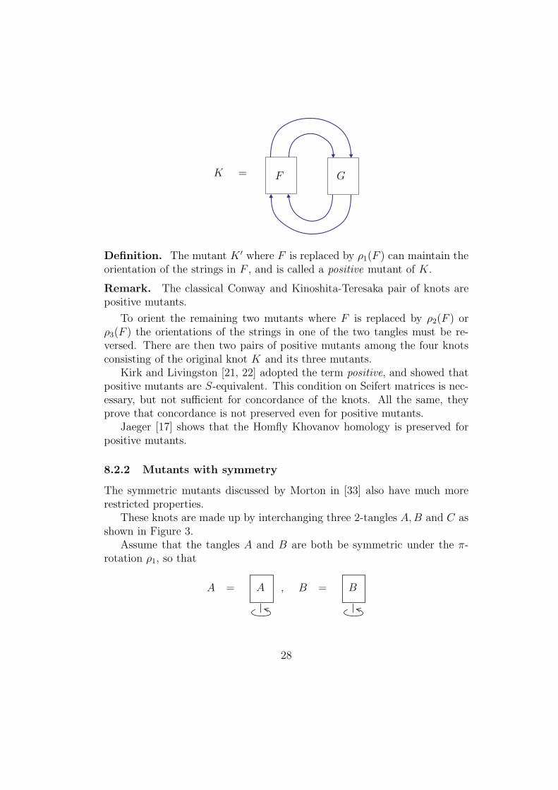
K = F G

Definition. The mutant K ′ where F is replaced by ρ1(F ) can maintain theorientation of the strings in F , and is called a positive mutant of K.

Remark. The classical Conway and Kinoshita-Teresaka pair of knots arepositive mutants.

To orient the remaining two mutants where F is replaced by ρ2(F ) orρ3(F ) the orientations of the strings in one of the two tangles must be re-versed. There are then two pairs of positive mutants among the four knotsconsisting of the original knot K and its three mutants.

Kirk and Livingston [21, 22] adopted the term positive, and showed thatpositive mutants are S-equivalent. This condition on Seifert matrices is nec-essary, but not sufficient for concordance of the knots. All the same, theyprove that concordance is not preserved even for positive mutants.

Jaeger [17] shows that the Homfly Khovanov homology is preserved forpositive mutants.

8.2.2 Mutants with symmetry

The symmetric mutants discussed by Morton in [33] also have much morerestricted properties.

These knots are made up by interchanging three 2-tangles A, B and C asshown in Figure 3.

Assume that the tangles A and B are both be symmetric under the π-rotation ρ1, so that

A = A , B = B

28

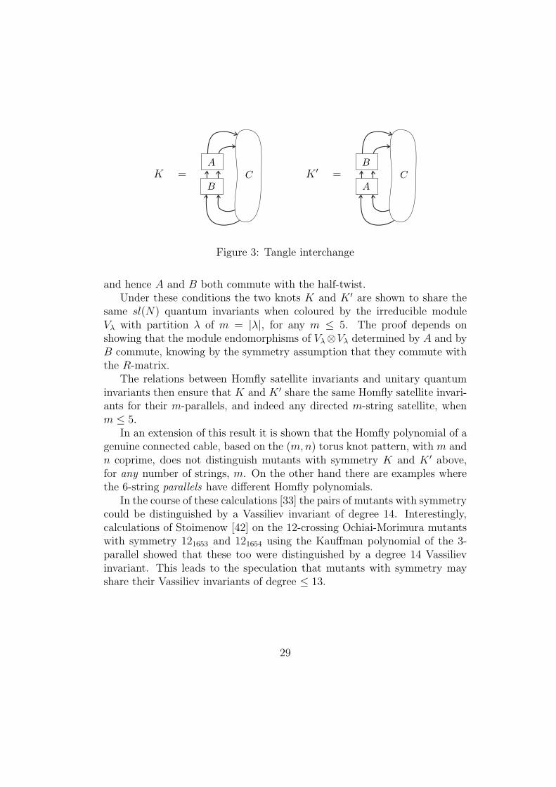
K =A

B

C K ′ =B

A

C

Figure 3: Tangle interchange

and hence A and B both commute with the half-twist.Under these conditions the two knots K and K ′ are shown to share the

same sl(N) quantum invariants when coloured by the irreducible moduleVλ with partition λ of m = |λ|, for any m ≤ 5. The proof depends onshowing that the module endomorphisms of Vλ⊗Vλ determined by A and byB commute, knowing by the symmetry assumption that they commute withthe R-matrix.

The relations between Homfly satellite invariants and unitary quantuminvariants then ensure that K and K ′ share the same Homfly satellite invari-ants for their m-parallels, and indeed any directed m-string satellite, whenm ≤ 5.

In an extension of this result it is shown that the Homfly polynomial of agenuine connected cable, based on the (m, n) torus knot pattern, with m andn coprime, does not distinguish mutants with symmetry K and K ′ above,for any number of strings, m. On the other hand there are examples wherethe 6-string parallels have different Homfly polynomials.

In the course of these calculations [33] the pairs of mutants with symmetrycould be distinguished by a Vassiliev invariant of degree 14. Interestingly,calculations of Stoimenow [42] on the 12-crossing Ochiai-Morimura mutantswith symmetry 121653 and 121654 using the Kauffman polynomial of the 3-parallel showed that these too were distinguished by a degree 14 Vassilievinvariant. This leads to the speculation that mutants with symmetry mayshare their Vassiliev invariants of degree ≤ 13.

29

References

[1] AK Aiston. Skein theoretic idempotents of Hecke algebras and quantumgroup invariants. PhD. thesis, University of Liverpool, 1996.

[2] AK Aiston and HR Morton. Idempotents of Hecke algebras of type A,J. Knot Theory Ramifications 7 (1998), 463–487.

[3] JS Birman and X-S Lin. Knot polynomials and Vassiliev’s invariants.Inventiones mathematicae 111 (1993), 225–270.

[4] JM Bloom. Odd Khovanov homology is mutation invariant. Math ResLett 17 (2010), 1–10.

[5] M Boileau, B Leeb and J Porti. Geometrization of 3-dimensional orb-ifolds. Ann. Math. 162 (2005), 195–290.

[6] F Bonahon and LC Siebenmann. The characteristic toric splitting ofirreducible compact 3-orbifolds. Math. Ann. 278 (1987), no. 1-4, 441–479.

[7] F Bonahon and LC Siebenmann. New geometric splittings of classi-cal knots and the classification and symmetries of arborescent knots.preprint 2010, Geometry and Topology Monographs, to appear.

[8] T Cochran and D Ruberman. Invariants of tangles. Math. Proc. Camb.Philos. Soc. 105 (1989), 299-306.

[9] JH Conway. On enumerations of knots and links, in Computational prob-lems in abstract algebra, ed. J Leech (Pergamon Press 1969), 329–358.

[10] D Cooper and WBR Lickorish. Mutations of links in genus 2 handle-bodies. Proc. Amer. Math. Soc. 127 (1999), 309–314.

[11] NM Dunfield, S Garoufalidis, A Shumakovitch and M Thistleth-waite. Behavior of knot invariants under genus 2 mutation.ArXiv:math/0607258 [math.GT].

[12] SV Chmutov, SV Duzhin and SK Lando. Vassiliev knot invariants. I.Introduction. Singularities and bifurcations, 117–126, Adv. Soviet Math.,21, Amer. Math. Soc., Providence, RI, 1994.

30

[13] R Fenn and C Rourke. Racks and links in codimension two. J. KnotTheory Ramifications 1 (1992) 343–406.

[14] RH Fox. A quick trip through knot theory, in Topology of 3-manifoldsand related topics, ed. MK Fort, Prentice-Hall, NJ, (1961), 120–167.

[15] D Gabai. Genera of the arborescent links. Memoirs Amer. Math. Soc.vol 59, number 339 (1986), 1–98.

[16] D Gabai. Foliations and genera of links. Topology 23 (1984), 381–394.

[17] TC Jaeger. Khovanov-Rozansky homology and Conway mutation.ArXiv:1101.3302.

[18] C Kearton. Mutation of knots. Proc. Amer. Math. Soc. 105 (1989), 206–208.

[19] S Kinoshita and H Terasaka. On unions of knots, Osaka Math. J., 9(1957), 131–153.

[20] S-G Kim and C Livingston. Knot mutation: 4-genus and algebraic con-cordance. Pacific J. Math. 220 (2005), 87–105

[21] P Kirk and C Livingston. Twisted knot polynomials: inversion, muta-tion and concordance. Topology 38 (1999), 663–671.

[22] P Kirk and C Livingston. Concordance and mutation. Geom. Topol. 5(2001), 831–883.

[23] WBR Lickorish. Prime knots and tangles. Trans. Amer. Math. Soc. 267(1981), 321–332.

[24] WBR Lickorish. Polynomials for links. Bull. London Math. Soc. 20(1988), 558–588.

[25] WBR Lickorish and AS Lipson. Polynomials of 2-cable-like links. Proc.Amer. Math. Soc. 100 (1987), 355–361.

[26] SG Lukac. Homfly skeins and the Hopf link. PhD thesis, University ofLiverpool 2001.

[27] HR Morton and PR Cromwell. Distinguishing mutants by knot polyno-mials. J. Knot Theory Ramifications 5 (1996), 225–238.

31

[28] HR Morton and PMG Manchon. Geometrical relations and plethysmsin the Homfly skein of the annulus. J. London Math. Soc. (2) 78 (2008)305–328.

[29] HR Morton and HJ Ryder. Mutants and SU(3)q invariants. In ‘Geom-etry and Topology Monographs’, Vol.1: The Epstein Birthday Schrift.(1998), 365–381.

[30] HR Morton and N Ryder. Invariants of genus 2 mutants. J.Knot TheoryRamifications 18 (2009) 1423–1438.

[31] HR Morton and HB Short. The 2-variable polynomial of cable knots.Math. Proc. Camb. Phil. Soc. 101 (1987), 267–278.

[32] HR Morton and P Traczyk. The Jones polynomial of satellite linksaround mutants. In ‘Braids’, ed. Joan S. Birman and Anatoly Libgober,Contemporary Mathematics 78, Amer. Math. Soc. (1988), 587–592.

[33] HR Morton. Mutant knots with symmetry. Math. Proc. Camb. Philos.Soc. 146 (2009), 95–107.

[34] Jun Murakami.The parallel version of polynomial invariants of links.Osaka J. Math. 26 (1989), 1–55.

[35] Jun Murakami. Finite type invariants detecting the mutant knots. In‘Knot Theory’. A volume dedicated to Professor Kunio Murasugi for his70th birthday. Ed. M. Sakuma et al., Osaka University, (2000), 258-267.

[36] L Paoluzzi. Hyperbolic knots and cyclic branched covers. Publ. Mat. 49(2005), 257–284.

[37] KA Perko. Invariants of 11-crossing knots. Prepublications Math.d’Orsay 80, Universite de Paris-Sud (1980).

[38] J Przytycki. Equivalence of cables of mutants of knots. Can. J. Math.XLI (1989), 250–273.

[39] R Riley. Homomorphisms of knot groups on finite groups. Math. Com-put. 25 (1971), 603-617.

32

[40] D Rolfsen. The quest for a knot with trivial Jones polynomial: diagramsurgery and the Temperley-Lieb algebra, in Topics in Knot Theory, M.E. Bozhuyuk, Kluwer Academic Publ., Dordrecht, 1993, 195-210.

[41] D Ruberman. Mutation and volume of knots in S3. Invent. Math. 90(1987), 189–215.

[42] A Stoimenow. Tabulating and distinguishing mutants. Int. J. Algebraand Computation 20 (2010), 525-559.

[43] VG Turaev. Quantum invariants of knots and 3-manifolds. De GruyterStudies in Mathematics, 18. Walter de Gruyter and Co., Berlin, 1994.

[44] OYa Viro. Non-projecting isotopies and knots with homeomorphic cov-ers. J. Soviet Math. 12 (1979) 86–96.This is a translation of his article LOMI Zapiski Nauchnykh Sem. 66(1976), 133-147.

[45] JR Weeks. SnapPea: a computer program for creating and studyinghyperbolic 3-manifolds, available fromhttp://thames.northnet.org/weeks/index/SnapPea.html

[46] H Wenzl. Quantum groups and subfactors of type B, C and D. Comm.Math. Phys. 133 (1990), 383–432.

33