MUON STOPPING POWER AND RANGE TABLES 10 …pdg.lbl.gov/2017/AtomicNuclearProperties/adndt.pdf · MUON STOPPING POWER AND RANGE TABLES 10 MeV|100 TeV DONALD E. GROOM ... Density e

D. E. GROOM, N. V. MOKHOV, and S. STRIGANOV Muon Stopping Power and Range

MUON STOPPING POWER AND RANGE TABLES

10 MeV—100 TeV

DONALD E. GROOM

Ernest Orlando Lawrence Berkeley National Laboratory1 Cyclotron Road, Berkeley, CA 94556, USA

[email protected]

and

NIKOLAI V. MOKHOV

Fermi National Accelerator LaboratoryBatavia, IL [email protected]

and

SERGEI I. STRIGANOV

Fermi National Accelerator LaboratoryBatavia, IL 60510

[email protected]

andIHEP, Protvino, [email protected]

The mean stopping power for high-energy muons in matter can be described by 〈−dE/dx〉 =a(E) + b(E)E, where a(E) is the electronic stopping power and b(E) is the energy-scaled con-tribution from radiative processes—bremsstrahlung, pair production, and photonuclear interac-tions. a(E) and b(E) are both slowly-varying functions of the muon energy E where radiativeeffects are important. Tables of these stopping power contributions and continuous-slowing-down-approximation (CSDA) ranges (which neglect multiple scattering and range straggling) are givenfor a selection of elements, compounds, mixtures, and biological materials for incident kinetic en-ergies in the range 10 MeV to 100 TeV. Tables of the contributions to b(E) are given for the samematerials.

LBNL-44742 1 Atomic Data and Nuclear Data Tables, Vol. 76, No. 2, July 2001


Contents

1. Introduction . . . . . . . . . . . . . . . . . . . . . . . . . . . . . . . . . . 3

2. Overview . . . . . . . . . . . . . . . . . . . . . . . . . . . . . . . . . . . . 5

3. Electronic energy losses of high-energy heavy particles . . . . . . . . . . . . . . 7

3.1. Major contributions . . . . . . . . . . . . . . . . . . . . . . . . . . . . 7

3.2. Mean excitation energy . . . . . . . . . . . . . . . . . . . . . . . . . . 9

3.3. Low-energy corrections . . . . . . . . . . . . . . . . . . . . . . . . . . 9

3.4. Density effect . . . . . . . . . . . . . . . . . . . . . . . . . . . . . . . 11

3.5. Other high-energy corrections . . . . . . . . . . . . . . . . . . . . . . . 12

3.6. Bethe-Bloch equation . . . . . . . . . . . . . . . . . . . . . . . . . . . 13

3.7. Comparison with other ionizing energy loss calculations . . . . . . . . . . . 13

4. Radiative losses . . . . . . . . . . . . . . . . . . . . . . . . . . . . . . . . . 14

4.1. Bremsstrahlung . . . . . . . . . . . . . . . . . . . . . . . . . . . . . . 15

4.2. Direct e+e− pair production . . . . . . . . . . . . . . . . . . . . . . . . 16

4.3. Photonuclear interactions . . . . . . . . . . . . . . . . . . . . . . . . . 17

4.4. Comparison with other works on muon radiative losses . . . . . . . . . . . 19

4.5. Muon critical energy . . . . . . . . . . . . . . . . . . . . . . . . . . . 22

4.6. Fluctuations in radiative energy loss . . . . . . . . . . . . . . . . . . . . 22

5. Tabulated data . . . . . . . . . . . . . . . . . . . . . . . . . . . . . . . . . 23

Appendix A. Stopping power and density-effect parameters for compoundsand mixtures . . . . . . . . . . . . . . . . . . . . . . . . . . . . . . . . 30

Appendix B. Direct pair production from screened nuclei . . . . . . . . . . . . . . 32

Explanation of Tables . . . . . . . . . . . . . . . . . . . . . . . . . . . . . . . 37



1. Introduction

The mean stopping power for high-energy muons (or other heavy charged particles1) in a materialcan be described by [1]

〈−dE/dx〉 = a (E) + b (E)E , (1)

where E is the total energy, a(E) is the electronic stopping power, and b(E) is due to radiativeprocesses—bremsstrahlung, pair production, and photonuclear interactions:

b ≡ bbrems + bpair + bnucl (2)

The notation is convenient because a(E) and b(E) are slowly varying functions of E at the highenergies where radiative contributions are important. b(E)E is less than 1% of a(E) for E <∼100 GeV for most materials.

The “continuous-slowing-down-approximation” (CSDA) range is obtained from the integral

R (E) =

∫ E

E0

[a (E′) + b (E′)E′]−1

dE′ (3)

where E0 is sufficiently small that the result is insensitive to its exact value. At very high energies,where a and b are (essentially) constant,

R (E) ≈ (1/b) ln (1 + E/Eµc) , (4)

where Eµc = a/b is the muon critical energy. The muon critical energy can be defined more preciselyas the energy at which electronic losses and radiative losses are equal, in analogy to one of the waysof defining the critical energy for electrons. It is obtained by finding Eµc such that

a (Eµc) = Eµcb (Eµc) . (5)

The CSDA range is of limited usefulness, particularly at higher energies, because of the effect offluctuations. (Fluctuations in radiative losses are discussed briefly in Section 4.6.) For example, thecosmic ray muon intensity falls very rapidly with energy, so that the flux observed deep undergroundis quite different from that to be expected from Eq. (3). We nonetheless calculate the CSDA rangegiven by Eq. (3) as an indicator of actual muon range.

The important and well-studied subjects of stopping power fluctuations and range straggling inelectronic energy loss [2,3] are not treated, even though they are much more serious for muons thanfor heavier particles: The fractional range straggling (

√

variance(range)/range) scales as√

1/Mfor particles with the same velocity, and hence is three times larger for a 100 MeV muon thanfor a 900 MeV proton. In copper the fractional straggling varies from 4% at 10 MeV, through aminimum of 2.8% at 300 MeV, then rising through 5.7% at 10 GeV. Above ∼ 100 GeV stragglingdue to fluctuations in bremsstrahlung losses begins to dominate.

Multiple scattering is also neglected, but with more justification. One measure of multiplescattering is provided by the “detour factor” [3], the ratio of the average penetration depth to theaverage path length for a stopping particle. The detour factor is 0.98 in the worst case (uraniumat our lowest energy). This ratio increases rapidly toward unity as the energy is increased or if theatomic weight of the absorber is decreased.

1 The radiative loss formulae given in this paper apply only to a spin-1/2 pointlike heavy particles, where“heavy” means “much more massive than an electron.” Insofar as we know, the solution for spin-0 particleshas never been published.



Table 1: Definitions of most of the variables used in this report. The electroniccharge e and the kinematic variables β = v/c and γ = 1/

√1 − β2 have their usual

definitions. Constants are from CODATA Recommended Values of the Fundamen-

tal Physical Constants: 1998 [7]. Parenthetical numbers after the values givethe 1-standard deviation uncertainties in the last digits. In Sect. 4 the conventionc = 1 is used.

Symbol Definition Units or Value

α Fine structure constant e2/4πε0hc 1/137.035 999 76(50)M Incident particle mass MeV/c2

Mµ Muon mass 105.658 356 8(52) MeV/c2

E Incident particle energy γMc2 MeVT Kinetic energy (γ − 1)Mc2 MeVp Momentum γβMc MeV/c

mec2 Electron mass × c2 0.510 998 902(21) MeV

re Classical electron radius e2/4πε0mec2 2.817 940 285(31) fm

NA Avogadro’s number 6.022 141 99(47) × 1023 mol−1

ze Charge of incident particleZ Atomic number of mediumA Atomic mass of medium g mol−1

(Occasionally: atomic mass number) dimensionlessK/A 4πNAr2

emec2/A 0.307 075 MeV g−1 cm2 for A = 1 g mol−1

I Mean excitation energy eV (Nota bene! )δ Density effect correction to electronic energy loss

hωp Plasma energy√

4πNer3e mec

2/α 28.816√

ρ 〈Z/A〉 eV for ρ in g cm−3

Ne Electron densitywj Fraction by weight of the jth element in a compound or mixture (

∑

wi = 1)nj number of the jth kind of atoms in a compound or mixtureEµc Muon critical energy GeVν Fractional energy transfer in an incident particle interactionε νE, the energy transfer in a single interaction

Tables of muon energy loss from a 1985 CERN internal report by Lohmann, Kopp, and Voss [4]have become the de facto world standard. This careful work serves as the benchmark for thepresent effort. Later theoretical work enables us to improve the calculations for low-Z elements(2 ≤ Z ≤ 10) and to make minor improvements elsewhere.

It is our intention to make this report sufficiently self-contained that the interested user canreplicate our calculations, even though this results in our giving often-tedious detail. The necessaryconstants for electronic loss calculations and tables of b(E) for elements, for the mean radiative losscalculations, are also available as ASCII files at http://pdg.lbl.gov/AtomicNuclearProperties.These tables are more extensive than the subset of data actually presented in this paper.

There is one serious dilemma: We believe that the density effect corrections via the carefulparameterizations of Sternheimer et al. [5] are more dependable than those calculated via theirgeneral algorithm [6]. But, as will be discussed in Section 3.2, better values for mean excitationenergies are now available for a variety of materials. The changes are sometimes as great as 10%.Over much of our energy region of interest (for βγ >∼ 1000) however, the density effect has “replaced”the mean excitation energy by the plasma energy, so that improvements in the mean excitationenergy have no effect on the stopping power. We therefore continue to use sometimes-obsolete



excitation values. How this affects our results will be discussed in Section 3.2. On the other hand,corrections to the densities used by Sternheimer et al. [5] are easily accommodated if the changesare small; this is done in several cases.

We present tables of stopping power and mean range for muons from kinetic energy T = 10 MeVto 100 TeV for most elements and a variety compounds and mixtures. Tables of b(E) are given forthe same materials. In the case of elemental gases, tables are also given for the liquid state.

The symbols and constants used in this report are explained in Table 1.

2. Overview

The behavior of stopping power (= 〈−dE/dx〉) in copper over twelve decades of muon kinetic energyis shown by the solid curves in Fig. 1. Data below the breaks in the curves are from ICRU 49 [3],while data above the breaks are from our present calculations. Approximate boundaries betweenregions described by different theories or phenomenologies are indicated by the shaded verticalbands. While our main interest is at higher energies, some understanding of the behavior at lowerenergies is useful, in particular for starting range integrals.

For β < α, below the first grey band in Fig. 1, the muon velocity is small compared with thatof the valence electrons in the absorber. Following the work of Fermi and Teller [9], Lindhardand collaborators have constructed a successful semi-phenomenological model to describe ionizingenergy losses in this regime, approximating the electronic structure of solids by a Fermi electrongas distribution [10]. The stopping power is found to be proportional to the projectile velocity.This region is marked by the dashed curve with the dotted extension in Fig. 1. However, belowβ ≈ 0.001–0.01 nonionizing energy losses via nuclear recoil become increasingly significant [3],finally dominating energy loss at very low energies.

Above β ≈ 0.05 or 0.1 (the second grey band in Fig. 1) one may make the opposite approxima-tion, neglecting electronic motion within atoms. There is no satisfactory theory for the intermediateregion, α < β < 0.1 (but see Ref. 11). There is, however, a rich experimental literature, whichAndersen and Ziegler have used to construct phenomenological fits bridging the regions in whichthere is adequate theoretical understanding [12]. This is the interval between the grey bandsshown in Fig. 1.

Electronic (ionization + excitation) losses in the high-velocity region are well described byBethe’s theory based on a first-order Born approximation [13], to which are added a number ofcorrections for the low-energy region and to account for the polarization of the medium at highenergies. The curve falls to a broad minimum whose position for solid absorbers decreases fromβγ = 3.5 to 3.0 as Z goes from 7 to 100. The mean electronic loss at the minimum value as afunction of Z is shown in Fig. 2. The rise in Fig. 1 with further increases of the projectile energy(labeled “without δ” in Fig. 1) is less marked when the polarization effects are taken into account(dash-dotted curve).

Electronic losses at very high energies are somewhat modified by bremsstrahlung from theatomic electrons [14] (see Section 3.5) and other effects, such as form factor corrections [15].These are of decreased importance because radiative energy losses begin to be significant above afew hundreds of GeV for even intermediate-Z absorbers. For example, radiative losses in copperdominate above Eµc = 315 GeV. The radiative contribution, and hence the entire energy loss rate,increases nearly linearly with energy above 1 TeV or so.



0.1 1 10 100 1 10 100 1 10 100 1 10 100

Muon kinetic energy T

Muon momentum p

1

10

100

Stop

ping

pow

er [M

eV c

m2 /

g]

1

10

100

Stop

ping

pow

er [M

eV c

m2 /

g]

Lin

dhar

d-

Scha

rff

Lin

dhar

d-

Scha

rff

Andersen- Ziegler

Bethe-Bloch Radiative

Bethe-Bloch Radiative

Radiative effects

reach 1%

Radiative effects

reach 1%

µ+ on Cu

Without δ

Radiative losses

Without δ

Radiative losses

βγ0.001 0.01 0.1 1 10 100

1001010.1

1000 104 105 106

[MeV/c]100101

[GeV/c]100101

[TeV/c]

Andersen- Ziegler

Minimum ionization

Minimum ionization

Eµc

Eµc

Nuclear losses

[TeV][GeV][MeV][keV]

µ−

µ−

Nuclear losses

Figure 1: Stopping power (= 〈−dE/dx〉) for positive muons in copper as a func-tion of kinetic energy T (top figure, 12 orders of magnitude range) and as a functionof momentum p = Mβcγ (bottom figure, 9 orders of magnitude). Solid curves indi-cate the total stopping power. Data below the break at T ≈ 0.5 MeV are scaled bythe appropriate mass ratios from the π− and p tables in ICRU 49 [3], and data athigher energies are from the present calculations. Vertical bands indicate bound-aries between different theoretical approximations or dominant physical processes.The short dotted lines labeled “µ− ” illustrate the “Barkas effect” [8]. “Nuclearlosses” indicates non-ionizing nuclear recoil energy losses, which are negligible here.



0.5

1.0

1.5

2.0

2.5

⟨–dE

/dx⟩

min

(MeV

g–1

cm2 )

1 2 5 10 20 50 100Z

H He Li Be B CNO Ne SnFe

SolidsGases

H2 gas: 4.10 H2 liquid: 3.97

2.35 – 0.64 log10(Z)

Figure 2: Minimum ionization as a function of Z. The straight line is fitted forZ ≥ 6.

3. Electronic energy losses of high-energy heavy particles

The physics formulae needed to describe the average electronic energy losses of a high-energy(β � αZ) massive (6= electron) charged particle as it passes through matter have been reviewedelsewhere [3, 16–24]. ICRU 49 is particularly useful, although it is limited to protons and alphaparticles (except for a short π− table) and to proton energies less than 10 GeV, corresponding toE < 1.1 GeV for muons. In this energy region nuclear recoil contributes negligibly to energy loss,and radiative losses, which typically become important above tens of GeV, and radiative losses canbe added as an independent contribution.

For the moment, we leave open the possibilities that the charge is ze and that the particlemight be something other than a muon. We briefly review the subject here in order to emphasizehigh-energy behavior.

3.1. Major contributions

The electronic stopping power2 is calculated by summing the contributions of all possible inelasticscatterings. These are normally from lower to higher (bound or unbound) electronic energy states,so the particle loses a small amount of energy in each scattering. The kinetic energy of the scatteredelectron is Q.

In his derivation of the stopping power, Bethe [25] introduced the concept of “generalizedoscillator strength” which is closely related to the inelastic-scattering form-factor [20]. Thefollowing summarizes the detailed discussions by Rossi [17], Fano [19], and Bichsel [24].

1. Low-Q region. Here the reciprocal of the 3-momentum transfer (roughly an impact parameter)is large compared with atomic dimensions. The scattered electrons have kinetic energies up tosome cutoff Q1, typically 0.01–0.1 eV [17]. For this region, Bethe approximated the generalizedoscillator strength by the dipole oscillator strength f(ε) which is the generalized oscillator

2 Variously called S, a(E), or the electronic part of the total mean energy loss rate 〈−dE/dx〉.



strength f(ε, q) for zero momentum transfer q (ε is the energy loss in a single collision). f(ε)is closely related to the optical absorption coefficient. He derived the following contribution toS:

Slow =K

2z2 Z

A

1

β2

[

lnQ1

I2/2meβ2c2+ ln γ2 − β2

]

(6)

Here ln I =∫

f(ε) ln ε dε. The denominator I2/2meβ2c2 in the first (logarithmic) term is the ef-

fective lower cutoff on the integral over dQ/Q. This term comes from “longitudinal excitations”(the ordinary Coulomb potential), and the next two terms from transverse excitations.

The low-Q region is associated with large impact parameters and hence with long distances.Polarization of the medium can seriously reduce this contribution, particularly at high energieswhere the transverse extension of the incident particle’s electric field becomes substantial. Thecorrection is usually made by subtracting a density-effect term δ, inside the square brackets ofEq. (6). This important correction is discussed in Sect. 3.4.

2. Intermediate- and high-Q regions. In an intermediate region atomic excitation energies are notnecessarily small compared with Q, but transverse excitations can be neglected. At higherenergies Q can be equated to the energy given to the electron, neglecting its binding energy.When the integration of the energy-weighted cross sections is carried out from Q1 to someupper limit Qupper, one obtains

Shigh =K

2z2 Z

A

1

β2

[

lnQupper

Q1

− β2 Qupper

Qmax

]

. (7)

Here Qmax is the kinematic maximum possible electron recoil kinetic energy, given by

Qmax =2mec

2β2γ2

1 + 2γme/M + (me/M)2 . (8)

Qupper is normally equal to Qmax (as will be the case after the conclusion of this section), andcannot exceed Qmax. The more general form given in Eq. (7) is useful in considering restrictedenergy loss, which is of relevance in considering the energy actually deposited in a thin absorber.At high energies (such that Qupper/Qmax � 1) the first term in the square brackets dominates.If Qupper is restricted to some maximum value, e.g. 0.5 MeV, then Shigh is essentially constantfor Qmax > Qupper. If Qupper = Qmax the high-Q region stopping power rises with energy aslnQmax. In other words, the increase of Shigh with energy is associated with the production ofhigh-energy recoil electrons, or δ-rays.

A very small projectile mass dependence of the electronic stopping power is introduced byQmax, which otherwise depends only on projectile velocity.

In Fano’s discussion the low-energy approximation Qmax ≈ 2mec2β2γ2 = 2mep

2/M 2 is implicit.Accordingly, Eq. (7) is more closely related to Rossi’s form (see his Eqns. 2.3.6 and 2.5.4). Thislow-energy approximation is made in many papers of the Bevatron era, but is in error by afactor of two for a muon with T = 10.8 GeV. Note that Qmax → E at very high energies.



3.2. Mean excitation energy

“The determination of the mean excitation energy is the principal non-trivial task in the evaluationof the Bethe stopping-power formula” [26]. Recommended values have varied substantially withtime. Estimates based on experimental stopping-power measurements for protons, deuterons, andalpha particles and on oscillator-strength distributions and dielectric-response functions were givenin ICRU 37 [27]. These were retained in ICRU 49 [3], where a useful comparison with otherresults is given, and they are used in the EGS4 [28] electron/photon transport code. These values(scaled by 1/Z) are shown in Fig. 3. The error estimates are from Table 2 in Ref. 26. As can beseen, I/Z ' 10 ± 1 eV for elements heavier than sulphur.

The figure also shows Bichsel’s more recent determination of I for selected heavy elements [29].He estimates uncertainties from 1.5% to 5%; the 5% errors are shown. The change from the ICRU 37values is less than 7% in all of the 19 cases except for samarium (7.5%), tungsten (7.5%), bismuth(9.3%) and thorium (9.5%). In addition, the mean excitation energy for liquid water has beenmore recently determined to be 79.7 ± 0.05 eV [31], significantly higher than the ICRU 37 value,75.0 eV. This reference also gives mean excitation energies for a variety of biological materials ofinterest here. In addition, Leung has described further corrections to stopping power theory due torelativistic effects of the target electrons [32]. Such effects could increase the stopping power byas much as 2% for high-Z targets. Bichsel has observed that this would be equivalent to loweringthe mean excitation energy values for high-Z materials by as much as 10%.

We are strongly motivated to use the ICRU 37 mean excitation energies because of the avail-ability of density effect parameters based on these values [5], yet in many cases the more recentvalues are superior and should be used. To investigate the consequences of errors or changes in themean excitation energies, we ran a version of our code in which I was increased by 10% and no otherchanges were made. In the Tµ = 10–100 MeV region, the stopping power increased by somewhatover 1% for carbon and iron. For lead it decreased by 2.6%–1.4% over this energy range. Since wedid not modify the density-effect parameters, in particular C (see Eq. (12)), there was a residual≈ 0.4% at high energies. The density-effect correction essentially replaces I by the plasma fre-quency hωp for p/M >∼ 1000, so the stopping power is completely insensitive to I for T >∼ 100 GeV,or for the lower half of our stopping power tables. The range integral always has contributionsfrom lower-energy parts, but these also become increasingly insignificant as the energy increases.We therefore feel justified in using the older data, for which dependable density-effect parametersare available.

3.3. Low-energy corrections

The distant-collision contribution to the stopping power given by Eq. (6) was obtained by Bethe [25]with the approximation that the velocities of atomic electrons are small compared with that of theprojectile. More precisely, Bethe’s approximation was to replace the generalized oscillator strengthby the dipole oscillator strength f(ε) in obtaining this result. This leads to correction terms [16]which are different for each atomic shell. The “shell correction” for the jth shell is represented by−2Cj/Z, so that an additional term −C/Z = −∑Cj/Z appears in the square brackets of Eq. (6).Other ways to calculate the shell correction are discussed in Ref. 3. Unfortunately, the algorithmsare not easy for the non-expert to implement.

The shell correction is not important at the energies of interest in this report. For example,the stopping power correction is 0.3% for a 10 MeV muon in iron, and 3% in uranium. It fallsrapidly with increasing energy. But even at intermediate energies it plays a role in “starting” therange integral. To investigate its importance, and to compare our results with the proton stoppingpower and range-energy tables in ICRU 49 [3], we have used the simple but long-obsolete analytic



0 10 20 30 40 50 60 70 80 90 100 8

10

12

14

16

18

20

22

I adj

/Z (e

V)

Z

Barkas & Berger 1964

Bichsel 1992

ICRU 37 (1984) (interpolated values are not marked with points)

Figure 3: Mean excitation energies (divided by Z) as adopted in ICRU 37 [27](filled points). Those based on experimental measurements are shown by symbolswith error flags; the interpolated values are simply joined. The grey point is forliquid H2; the black point at 19.2 is for H2 gas. The open circles show more moderndeterminations by Bichsel [29]. The dotted curve is from the approximate formulaof Barkas [30].

approximation for the shell correction introduced by Barkas [30]: 3 The accuracy of our results isaddressed in Section 3.7.

In early Bevatron experiments Barkas et al. [8] found that negative pions had a somewhatgreater range than positive pions with the same (small) initial energy. This was attributed to adeparture from first-order Born theory [33], and is normally included by adding a term zL1(β)to the stopping-power formula. The effect has been measured for a number of negative/positiveparticle pairs, most recently for antiprotons/protons at the CERN LEAR facility [34]. It isillustrated by the µ− stopping-power segment shown in Fig. 1.

Bethe’s stopping power theory is based on a first-order Born approximation. To obtain Bloch’sresult, a term z2L2(β) is added if results accurate at low energies are desired.

These corrections are discussed in detail in ICRU 49, and are mentioned here for completeness.They are not significant at the energies of concern in this report.

3 Explicitly,C =

(

0.422377η−2 + 0.0304043η−4 − 0.00038106η−6)

× 10−6I2

+(

3.858019η−2 − 0.1667989η−4 + 0.00157955η−6)

× 10−9I3 ,(9)

where η = βγ and I is in eV. This form is reasonably good only for η > 0.13 (T = 7.9 MeV for a proton,0.89 MeV for a muon).



3.4. Density effect

As the particle energy increases its electric field flattens and extends, so that the distant-collisionpart of dE/dx (Eq. (6)) increases as lnβγ. However, real media become polarized, limiting thisextension and effectively truncating part of this logarithmic rise. This “density effect” has beenextensively treated over the years; see Refs. 5, and 6, and 28, and references therein. The approachis to subtract a density-effect correction, δ, from the distant-collision contribution, resulting in theδ/2 term in Eq. (15). At very high energies,

δ/2 → ln (hωp/I) + lnβγ − 1/2 , (10)

where hωp is the plasma energy defined in Table 1. As can be seen from Eq. (15), the effect ofEq. (10) is to replace I with hωp and to eliminate the explicit β2γ2 dependence in the first (log)term in the square brackets. The remaining rise of the electronic stopping power comes from Qmax,given by Eq. (8). The effect of the density correction is shown in Fig. 1.

At some low energy (related to x0 below) the density effect is insignificant, and above some highenergy (see x1 below) it is well described by the asymptotic form given in Eq. (10). Conductorsrequire special treatment at the low-energy end. Sternheimer has proposed the parameterization [35]

δ =

2 (ln 10) x − C if x ≥ x1;

2 (ln 10) x − C + a (x1 − x)k

if x0 ≤ x < x1;0 if x < x0 (nonconductors);δ010

2(x−x0) if x < x0 (conductors) ,

(11)

where x = log10(p/M) = log10 βγ. C is obtained by equating the high-energy case of Eq. (11) withthe limit of Eq. (10), so that

C = 2 ln (I/hωp) + 1 . (12)

The other parameters (a, k, x0, x1, and δ0) are adjusted to give a best fit to the results of detailednumerical calculations for a logarithmically spaced grid of energy values. Note that C is the negativeof the C used in earlier publications. A variety of different parameter sets are available. In somecases these result from a different fitting procedure having been used with the same model, andalthough the parameters look different the resulting δ is not sensibly different. For elements, thePEGS4 data [28] use the values from Ref. 36.

In a series of papers by Sternheimer, Seltzer, and Berger, the density-effect parameter tablesare extended to nearly 300 elements, compounds, and mixtures. The chemical composition of thematerials is given in Ref. 26.4 The agreement with more detailed calculations or results obtainedwith other parameter sets is usually at the 0.5% level [37]; however, see Table IV in Ref. 38. Weuse the tables given in Ref. 5 for most of the present calculations.5

The densities used in these tables are occasionally in error, or, in the case of some polymerswith variable density, out of the usual range. In this and other cases we use Eq. (A.8) [6] to adjustthe parameters; these are marked by footnotes in the tables in Section 5.

4 Slightly incorrect compositions (and therefore density effect parameters) are given for lanthanum oxy-sulfide (corrected in a footnote in Ref. 37), cellulose acetate, cellulose nitrate, polypropylene, and perhapsother materials. These will be corrected, and an approximately equal number of new materials added, in aforthcoming publication [39].

5 Given the power of modern computers, experts now calculate the density effect from first principlesrather than use these formulae [39]. One problem along the way is knowing the mean excitation energy,which can be different for condensed and gas states of the same substance and even depends upon density. Inour case radiative effects dominate over most of the relevant energy range, and no great error is engenderedby employing the user-friendly parameterized forms.



There remains the problem of obtaining the density-effect parameters if they have not beentabulated for the material of interest. This issue is of particular importance here in the case ofcryogenic liquids such as N2, but is also of interest when dealing with a compound or mixture nottabulated by Sternheimer, Berger, and Seltzer [5]. The algorithm proposed by Sternheimer andPeierls [6] is discussed in Appendix A.

To some degree, both the adjustment of the parameters for a different density and the Stern-heimer–Peierls algorithm can be checked by using those cases in the tables where parameters aregiven for different densities of the same material. When the “compact carbon” parameters areadjusted to the two other tabulated carbon densities, the difference in stopping power and rangewith those obtained directly is less than 0.2%. Calculation of parameters for a cryogenic liquidusing the Sternheimer-Peierls algorithm can be checked for hydrogen and water. This method wasused to calculate parameters for liquid hydrogen at bubble chamber density (0.060 g/cm3), usingthe excitation energy for the liquid; at worst, at minimum ionization, 〈−dE/dx〉 was low by 2.5%,while the range was high by 1.1%. Deviations were smaller elsewhere. When the algorithm wasused to calculate parameters for water using the excitation energy for steam, the result was 1%higher at minimum ionization than that obtained directly with the water parameters. Only a slightimprovement was obtained by using the excitation energy given for water.

Hydrogen is always a worst case. Sternheimer, Berger, and Seltzer [5] tabulate parametersfor both hydrogen gas and liquid hydrogen under bubble chamber conditions, so we have madecalculations in both directions via the Sternheimer-Peierls algorithm and by scaling densities viaEq. (A.8). We conclude that the stopping power results in this report obtained with parametersscaled to different densities are accurate to within the overall 0.5% agreement level estimated bySeltzer and Berger [37], and that the parameters calculated for cryogenic liquids (except hydrogen)using the Sternheimer-Peierls algorithm could produce stopping power errors of slightly over 1% atminimum ionization, and less elsewhere.

3.5. Other high-energy corrections

Bremsstrahlung from atomic electrons in the case of incident muons was considered in a 1997 paperby Kelner, Kokoulin, and Petrukhin [14]. There are four lowest-order diagrams: Photon emissionby the muon before and after photon exchange with the electron, and emission by the electronbefore and after photon exchange. The former diagrams result in losses nearly proportional to E,and are described by Eq. (19). The latter are properly part of electronic losses, and produce anadditional term in the stopping power. To leading powers in logarithms, this loss is given by:

∆

∣

∣

∣

∣

dE

dx

∣

∣

∣

∣

=K

4π

Z

Aα

[

ln2E

Mµc2− 1

3ln

2Qmax

mec2

]

ln2 2Qmax

mec2(13)

As Kelner et al. observe, this addition is important at high energies, amounting to 2% of theelectronic loss at 100 GeV and 4% at 1 TeV. It is included in our calculations.

An additional spin-correction term, (1/4)(Qmax/E)2, is included in the square brackets Eq. (7)if the incident particle is a muon (point-like and spin 1/2) [17]. Its contribution to the stoppingpower asymptotically approaches 0.038 (Z/A) MeV g−1cm2, reaching 90% of that value at 200 GeVin most materials. In iron its fractional contribution reaches a maximum of 0.75% at 670 GeV.Although this contribution is well within uncertainties in the total stopping power, its inclusionavoids a systematic bias.

At energies above a few hundred GeV, the maximum 4-momentum transfer to the electron canexceed 1 GeV/c, so that, in the case of incident pions, protons, and other hadrons, cross sectionsare modified by the extended charge distributions of the projectiles. One might expect this “soft”



cutoff to Qmax to reduce the electronic stopping power. This problem has been investigated byJ. D. Jackson [15], who concluded that corrections to dE/dx become important only at energieswhere radiative losses dominate. At lower energies the stopping power is almost unchanged, sinceits average, dominated by losses due to many soft collisions, is insensitive to the rare hard collisions.For muons the spin correction replaces this form-factor correction.

Jackson and McCarthy [40] have pointed out that the Barkas correction calculated by Fermi(but see their Ref. 20) persists at high energies; hence, a term should be added to the close-collisionpart of Eq. (15):

Kz3 Z

A

πα

2β(14)

This correction, which is ±0.00176 MeV g−1 cm2 for z = ±1, Z/A = 1/2 and β = 1, producesrange differences of a few parts per thousand between positive and negative muons near minimumionization. At higher energies sign-indifferent radiative effects dominate. We neglect this correction.

3.6. Bethe-Bloch equation

We summarize this discussion with the Bethe-Bloch equation for muons in the form used in thispaper:

⟨

−dE

dx

⟩

electronic

= KZ

A

1

β2

[

1

2ln

2mec2β2γ2Qmax

I2− β2 − δ

2+

1

8

Q2max

(γMc2)2

]

+ ∆

∣

∣

∣

∣

dE

dx

∣

∣

∣

∣

(15)

The final term, for bremsstrahlung from atomic electrons, is given by Eq. (13).

Except for the very small projectile mass dependence introduced by Qmax, this expressiondepends only on the projectile velocity. This means that a value of the stopping power for aparticle with mass M1 and kinetic energy T1 is the same as the stopping power for a particle withmass M2 at T2 = (M2/M1)T1. Similarly, R/M is a function of T/M (or E/M , or p/M).

3.7. Comparison with other ionizing energy loss calculations

Comparisons with the ICRU 49 proton tables have been made by running our code with the protonmass. A summary of the stopping power comparisons is given in Table 2, and of the CSDA rangecomparisons in Table 3. In general the agreement is regarded as adequate, but is worse at highatomic number and low energy. The simple shell correction given by Eq. (9) has been used, andunder these conditions somewhat overcorrects.

ICRU 49 concludes that the “differences between tabulated and experimental stopping powersare mostly smaller than 1% and hardly ever greater than 2%,” and in the case of compounds andmixtures “the uncertainties are approximately three times as large as in the case of elements” [3].

Our muon tables start at T = 10 MeV, corresponding to a proton energy of about 100 MeV,so that only 100 MeV and above is relevant in the proton comparisons. For uranium the stoppingpower at 100 MeV is low by 0.8% and the range high by 1.9%. Without the shell correction thestopping power for this case is high by 1.7% and the range low by 2.5%. We make the shell correctiononly for elements. We conclude that in a worst-case scenario, PuCl4 (which we do not tabulate)at 10 MeV, our results could be in error by nearly 3%. For lower-Z materials the agreement isconsistent with ICRU 49. In any case the agreement improves rapidly with increasing energy.

Lohmann et al. [4] list muon electronic losses separately for hydrogen, iron, and uranium. Sincethey do not consider the contributions of bremsstrahlung from atomic electrons (Eq. (13)), we havemade comparisons with this correction “turned off.” Under these conditions, our results disagree



Table 2: Comparison of stopping power calculations for protons (in MeV g−1 cm2)with those of ICRU 49 [3] and Bichsel 1992 [29].

10 MeV 100 MeV 1 GeV 10 GeV

Hydrogen gas (Z = 1)This calculation 101.7 15.29 4.496 4.539ICRU 49 101.9 15.30 4.497 4.539

Graphite (Z = 6, ρ = 1.7 g/cm3)

This calculation 40.72 6.514 1.942 1.883ICRU 49 40.84 6.520 1.946 1.881

Iron (Z = 26)This calculation 28.54 5.045 1.575 1.603ICRU 49 28.56 5.043 1.574 1.601

Tin (Z = 50)This calculation 22.26 4.177 1.351 1.426ICRU 49 22.02 4.165 1.349 1.423

Lead (Z = 82)This calculation 17.52 3.532 1.189 1.291ICRU 49 17.79 3.552 1.186 1.288Bichsel 1992 17.79 3.592

Uranium (Z = 92)This calculation 16.68 3.388 1.144 1.243ICRU 49 16.90 3.411 1.140 1.242Bichsel 1992 16.86 3.450

Liquid waterThis calculation 45.94 7.290 2.210 2.132ICRU 49 45.67 7.289 2.211 2.126

by at most 2 in the 4th decimal place, presumably from different rounding of the density-effectparameters.

4. Radiative losses

The radiative contribution to muon stopping power is conveniently written as b(E)E [1], whereb(E) is a slowly-varying function of energy which is asymptotically constant. As indicated earlier,it is usually written as a sum of contributions from bremsstrahlung, direct pair production, andphotonuclear interactions:

b ≡ bbrems + bpair + bnucl (2)

Here we describe the calculation of these contributions. Note that the convention c = 1 is used inall the formulae in this section.

In this section we specialize to M = Mµ, although the results apply to any massive spin-1/2pointlike particle. To a very rough approximation, the bremsstrahlung contribution scales as 1/M 2,and the pair-production part as 1/M . The results below probably apply fairly well to charged pionradiative energy losses, although to the best of our knowledge radiative losses by spin-0 particleshas not been treated.



Table 3: Comparison of CSDA range calculations for protons (in g cm−2) withthose of ICRU 49.

10 MeV 100 MeV 1 GeV 10 GeV

Hydrogen gasThis calculation 0.0534 3.636 158.7 2254.ICRU 49 0.0535 3.633 158.7 2254.

Graphite (Z = 6, ρ = 1.7 g/cm3)

This calculation 0.1361 8.634 367.4 5333.ICRU 49 0.1377 8.627 367.0 5337.

Iron (Z = 26)This calculation 0.2013 11.36 459.2 6383.ICRU 49 0.2064 11.37 459.6 6389.

Tin (Z = 50)This calculation 0.2623 13.90 540.9 7272.ICRU 49 0.2764 13.95 541.9 7291.

LeadThis calculation 0.3315 16.79 620.7 8120.ICRU 49 0.3528 16.52 621.7 8143.

UraniumThis calculation 0.3462 17.56 645.2 8432.ICRU 49 0.3718 17.24 646.8 8456.

Liquid waterThis calculation 0.1201 7.710 325.4 4703.ICRU 49 0.1230 7.718 325.4 4700.

4.1. Bremsstrahlung

The cross section for electron bremsstrahlung was obtained by Bethe and Heitler [41]. In the caseof muons, it is necessary to take into account nuclear screening, which was first done consistentlyby Petrukhin and Shestakov [42]. A simple approximation for medium and heavy nuclei (Z > 10)was derived. Lohmann, Kopp, and Voss [4] also used this approximation, but for Z < 10 they setthe nuclear screening correction equal to zero. As a result, their bremsstrahlung contribution forlow-Z nuclei is overestimated by about 10%.

The CCFR collaboration [43] revised the Petrukhin and Shestakov [42] results, pointing outthat Ref. 42 overestimates the nuclear screening correction by about 10%. Kelner et al. [44] laterobserved that the CCFR conclusion probably resulted from an incorrect treatment of the Bethe-Heitler formula. Their new calculations were in good agreement with the old ones by Petrukhinand Shestakov for medium and heavy nuclei, but in addition they proposed an approximation forlight nuclei. An independent analysis was performed by the Bugaev group (see, e.g., Ref. 45). Theresults of Petrukhin and Shestakov and the Bugaev group for bremsstrahlung on screened nucleiagree to within a few percent.

All of the results mentioned above were derived in the Born approximation. It was recentlyshown [45] that the non-Born corrections in the region of low and high momentum transfers havethe same order of magnitude but opposite signs. As a consequence, they nearly compensate eachother.



The differential cross section for muon bremsstrahlung from a (screened) nucleus as given inRef. 44 is used for the present paper:

dσ

dν

∣

∣

∣

∣

brems, nucl

= α

(

2Zme

Mµ

re

)2 (4

3− 4

3ν + ν2

)

Φ(δ)

ν(16)

Here ν is the fraction of the muon’s energy transferred to the photon, and

Φ (δ) = ln

(

BMµZ−1/3/me

1 + δ√

e BZ−1/3/me

)

− ∆n (δ) , (17)

where Dn = 1.54A0.27, B = 182.7 (B = 202.4 for hydrogen), e = 2.7181 . . ., δ = M 2µν/2E(1 − ν),

and the nuclear screening correction ∆n is given by

∆n = ln

(

Dn

1 + δ (Dn

√e − 2) /Mµ

)

. (18)

The Thomas-Fermi potential for atomic electrons is assumed. A more precise calculation of theradiation logarithm using the Hartree-Fock model is described in Ref. 46, and the results agreewith the Thomas-Fermi results within about 1% at high energies (total screening); the agreementis better at low energies. Since there is not yet a Hartree-Fock result for screening in the case ofbremsstrahlung from atomic electrons, we prefer to use the form factors based on the Thomas-Fermipotential throughout.

To account for bremsstrahlung losses on atomic electrons, Z 2 in Eq. (16) is usually replacedwith Z(Z + 1) (e.g., see Ref. 4). A much better approximation for the contribution from electrons,taking into account electronic binding and recoil, is given by [14]:

dσ

dν

∣

∣

∣

∣

brems, elec

= αZ

(

2me

Mµ

re

)2 (4

3− 4

3ν + ν2

)

Φin (δ)

ν(19)

In this case

Φin (δ) = ln

(

Mµ/δ

Mµδ/m2e +

√e

)

− ln

(

1 +me

δ BZ−2/3√

e

)

, (20)

where B = 1429 for all elements but hydrogen, where B = 446, and δ = M 2ν/2E(1− ν), as above.

The cross section for bremsstrahlung as a function of fractional energy transfer ν is shown inFig. 4. Although pair production dominates the radiative contributions to the stopping power,bremsstrahlung dominates at high ν.

The average energy loss 〈−dE/dx〉 due to bremsstrahlung is calculated by integrating the sumof these cross sections, as in Eq. (21) below.

4.2. Direct e+e− pair production

The cross section for direct e+e− pair production in a Coulomb field was first calculated byRacah [47]. Atomic screening was later taken into account by Kelner and Kotov [48]. With theirapproach, the average energy loss is obtained through a three-fold numerical integration. Withthe simple parameterization of the screening functions proposed by Kokoulin and Petrukhin [49],one obtains a double differential cross section for e+e− production. This formula is widely used inmuon transport calculations (for example, see Ref. 4). Based on this work, a (rather complicated)analytic form for the energy spectrum of pairs created in screened muon-nucleus collisions was



derived by Nikishov [50]. The explicit formula is given in Appendix B. The average energy lossfor pair production is calculated by numerical integration:

bpair, nucl = − 1

E

dE

dx

∣

∣

∣

∣

pair, nucl

=NA

A

∫ 1

0

νdσ

dνdν (21)

The same expression as for the nucleus is usually used to calculate the pair production con-tribution from atomic electrons, with Z 2 replaced with Z (e.g., Ref. 4). A more precise approachhas recently been developed by Kelner [51], who proposed a simple parameterization of the energyloss based on a rigorous QED calculation. This formula for the electronic contribution to pairproduction energy loss by muons is valid to within 5% of the more laborious numerical result forE > 5 GeV, and is used for the present calculations:

bpair, elec = − 1

E

dE

dx

∣

∣

∣

∣

pair, elec

=Z

A

(

0.073 ln

(

2E/Mµ

1 + g Z2/3E/Mµ

)

− 0.31

)

× 10−6cm2/g (22)

Here g = 4.4 × 10−5 for hydrogen and g = 1.95 × 10−5 for other materials.

The cross section for direct pair production as a function of fractional energy transfer ν isshown in Fig. 4.

4.3. Photonuclear interactions

Several approaches have been developed to calculate the muon photonuclear cross section. Themost widely used is that of Bezrukov and Bugaev [52]:

dσ

dν

∣

∣

∣

∣

nucl

=α

2πAσγN (ε) ν

{

0.75G (x)

[

κ ln

(

1 +m2

1

t

)

− κm21

m21 + t

− 2M 2µ

t

]

+ 0.25

[

κ ln

(

1 +m2

2

t

)

−2M 2

µ

t

]

+M 2

µ

2t

[

0.75G (x)m2

1

m21 + t

+ 0.25m2

2

tln

(

1 +t

m22

)]}

(23)

Here ε is the energy loss of the muon and σγN(ε) is the photoabsorption cross section defined below.Other values are given by

ν =ε

E, t =

M 2µν2

1 − ν, κ = 1 − 2

ν+

2

ν2, and G (x) =

3

x3

(

x2

2− 1 + e−x (1 + x)

)

, (24)

x = 0.00282A1/3σγN(ε), m21 = 0.54 GeV2, and m2

2 = 1.8 GeV2. This cross section gives resultsconsistent with other calculations to within 30% [4]. Recent measurements of photonuclearinteraction of muon in rock performed by the MACRO collaboration [53] agree quite well withMonte Carlo simulations based on the Bezrukov and Bugaev cross section.

The total cross section σγN(ε) for the photon-nucleon interaction appears as a normalizationparameter in Ref. 52, which proposes a simple parameterization:

σγN (ε) (in µb) = 114.3 + 1.647 ln2 (0.0213 ε) (25)

This approximation is good enough only for muon energy loss ε > 5 GeV. For smaller ε, we usethe experimental data given by Armstrong et al. [54]. The energy loss contribution is calculatedby numerical integration of the differential cross section given by Eq. (23). The use here of a moreprecise photo-absorption cross section for ε < 5 than was used in the original model [52] does notchange the photonuclear part of 〈−dE/dx〉 appreciably.

The cross section for photonuclear interactions as a function of fractional energy transfer ν isshown in Fig. 4.



Total (including ionization)



10 GeV/c µ– on iron

100 GeV/c µ– on iron

1 TeV/c µ– on iron

10 TeV/c µ– on iron

Fractional energy transfer ν Fractional energy transfer ν

dσ/d

ν (

cm2 /

g)dσ

/dν

(cm

2 /g)

10–5 10–4 10–3 0.01 0.1 10–4 10–3 0.01 0.1 1.0

Pair

PairPair

BremsBrems

Brems

Brems


Photonuclear

Photonuclear

Photonuclear

Photo- nuclear

10–5

10–6

10–7

10–4

10–3

0.01

0.1

1.0

10.0

100.0

10–7

10–6

10–5

10–4

10–3

0.01

0.1

1.0

10.0

100.0

103

104

Pair

Figure 4: Differential cross section for total and radiative processes as a functionof the fractional energy transfer for muons on iron.



Table 4: Comparison of btot calculations with those deduced from Lohmann etal. [4] and, in the case of standard rock, with Gaisser and Stanev [55]. btot islisted in units of 10−6 g−1 cm2.

Total energy = 10 GeV 100 GeV 1 TeV 10 TeV 100 TeV

HydrogenThis calculation 0.941 1.345 1.773 2.079 2.284Lohmann et al. 1.081 1.463 1.814 2.046 —

CarbonThis calculation 1.278 1.972 2.548 2.859 3.030*Lohmann et al. 1.3 2.14 2.679 2.958 —

IronThis calculation 3.290 5.701 7.392 8.110 8.371Lohmann et al. 3.312 5.795 7.444 8.128 —

UraniumThis calculation 8.234 14.614 18.747 20.308 20.760Lohmann et al. 8.046 14.790 18.870 20.360 —

WaterThis calculation 1.439 2.279 2.959 3.313 3.497*Lohmann et al. 1.5 2.49 3.125 3.459 —

Standard rockThis calculation 1.840 3.028 3.934 4.365 4.563*Lohmann et al. 1.8 3.10 3.960 4.361 —Gaisser & Stanev 1.91 3.12 4.01 4.40 —

OxygenThis calculation 1.502 2.397 3.108 3.468 3.650*Lohmann et al. 1.6 2.62 3.290 3.620 —

* Obtained from the Lohmann et al. energy loss tables assuming our values forelectronic losses (without the bremsstrahlung correction given by Eq. (13)).The subtraction loses significance at 10 GeV, where the radiative contributionis small.

4.4. Comparison with other works on muon radiative losses

Selected b values from our present calculations and according to Lohmann et al. [4] are listed inTable 4 and plotted in Fig. 5 as a function of muon energy. Since Lohmann et al. did not give thedecomposition of the stopping powers except for H, Fe, and U, values of btot for the materials givenin the right half of the figure were obtained by assuming our values of the ionizing losses (withoutthe bremsstrahlung correction given by Eq. (13), which was omitted in Ref. 4). This is justifiedbecause for the fiducial cases H, Fe, and U our results agree with their values to within roundingerrors in the 4th place.

For Z > 10 the results are nearly identical. For smaller atomic number, and at low energies,two effects are responsible for the differences:

1. In the nuclear part of bremsstrahlung, nuclear screening has only a weak energy dependence,and produces about a 4% reduction for hydrogen and a 10% reduction for carbon. This isapparent in our lower values of btot for carbon and water as compared with Lohmann et al.

2. The cross sections for bremsstrahlung and pair production from atomic electrons decrease atlow energies because of electron recoil. In our calculations Lohmann et al.’s Z(Z + 1) factor is



0.0

0.5

1.0

1.5

2.0

2.5

Hydrogen Z = 1

Iron Z = 26

0.0

0.5

1.0

1.5

2.0

2.5

3.0

3.5

Carbon Z = 6

0

2

4

6

8Water

0

5

10

15

20

Uranium Z = 92

0

1

2

3

4

Muon energy (GeV)

106

b(E

) (g

−1cm

2 )

106

b(E

) (g

−1cm

2 )

106

b(E

) (g

−1cm

2 )

106

b(E

) (g

−1cm

2 )

106

b(E

) (g

−1cm

2 )

106

b(E

) (g

−1cm

2 )

btot

bpair

bnuc

btot

bpair

bbrems

bnuc

btot

bpair

bbrems

bnuc

100102 1000 104 105

Muon energy (GeV)100102 1000 104 105

btot

bpair

bbrems

bnuc

btot

bpair

bbrems

bnuc

btot

bpair

bbrems

bnuc

Standard rock

0

1

2

3

bbrems

Figure 5: b-values for a sampling of materials. Solid lines represent our results,while the dashed/dotted lines are from Lohmann et al. [4]. The circles forstandard rock are from Gaisser and Stanev [55].



replaced by Z(Z+0) in the low-energy limit, so that for hydrogen our contributions to these pro-cesses for 1–10 GeV are smaller by nearly a factor of two. Similarly, in the low-energy limit ourbremsstrahlung and pair production contributions for carbon are 6/7 of Lohmann et al.’s values.

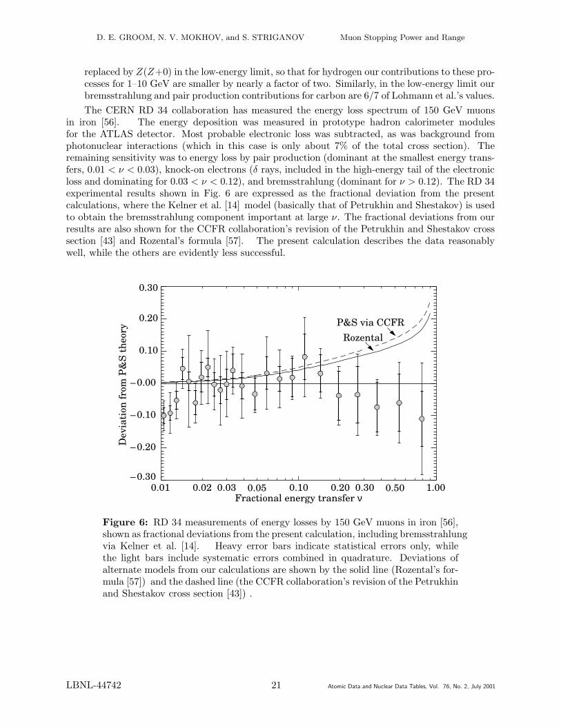
The CERN RD 34 collaboration has measured the energy loss spectrum of 150 GeV muonsin iron [56]. The energy deposition was measured in prototype hadron calorimeter modulesfor the ATLAS detector. Most probable electronic loss was subtracted, as was background fromphotonuclear interactions (which in this case is only about 7% of the total cross section). Theremaining sensitivity was to energy loss by pair production (dominant at the smallest energy trans-fers, 0.01 < ν < 0.03), knock-on electrons (δ rays, included in the high-energy tail of the electronicloss and dominating for 0.03 < ν < 0.12), and bremsstrahlung (dominant for ν > 0.12). The RD 34experimental results shown in Fig. 6 are expressed as the fractional deviation from the presentcalculations, where the Kelner et al. [14] model (basically that of Petrukhin and Shestakov) is usedto obtain the bremsstrahlung component important at large ν. The fractional deviations from ourresults are also shown for the CCFR collaboration’s revision of the Petrukhin and Shestakov crosssection [43] and Rozental’s formula [57]. The present calculation describes the data reasonablywell, while the others are evidently less successful.

0.01 0.02 0.03 0.05 0.20 0.30 0.500.10 1.00Fractional energy transfer ν

–0.30

–0.20

–0.10

–0.00

0.10

0.20

0.30

Dev

iati

on fr

om P

&S

theo

ry

RozentalP&S via CCFR

Figure 6: RD 34 measurements of energy losses by 150 GeV muons in iron [56],shown as fractional deviations from the present calculation, including bremsstrahlungvia Kelner et al. [14]. Heavy error bars indicate statistical errors only, whilethe light bars include systematic errors combined in quadrature. Deviations ofalternate models from our calculations are shown by the solid line (Rozental’s for-mula [57]) and the dashed line (the CCFR collaboration’s revision of the Petrukhinand Shestakov cross section [43]) .



4.5. Muon critical energy

Equation (5) defines the muon critical energy Eµc as the energy for which electronic and radiativelosses are equal. Eµc for the chemical elements is shown in Fig. 7. The equality of electronicand radiative losses comes at a higher energy for gases than for solids and liquids because of thesmaller density-effect correction for gases. Empirical functions have been fitted to these data forgases and for solids/liquids, in both cases excluding hydrogen from the fits. Since Eµc dependsupon ionization potentials and density-effect parameters as well as Z, the fits cannot be exact.Potassium, rubidium, and cesium are 3.6%, 3.2% and 3.4% high, respectively, while beryllium is3.8% low. Most of the other solids and liquids fall within 2.5% of the fitted function. Among gasesthe worst fit is for neon (1.9% high).

100

200

400

700

1000

2000

4000

Eµc

(GeV

)

1 2 5 10 20 50 100Z

7980 GeV_____________ (Z + 1.94)0.885

6590 GeV_____________ (Z + 1.92)0.880

H He Li Be B CNO Ne SnFe

SolidsGases

Figure 7: Muon critical energy for the chemical elements. As discussed in thetext, the fitted functions shown in the figure cannot be exact, and are for guidanceonly.

4.6. Fluctuations in radiative energy loss

The radiative cross sections at several energies are shown in Fig. 4. The bremsstrahlung crosssection varies roughly as 1/ν over most of the range (where ν is the fraction of the muon’s energytransferred in a collision), while for pair production the distribution varies as ν−3 to ν−2 (see alsoRef. 58). “Hard” losses are therefore more probable in bremsstrahlung, and in fact energy lossesdue to pair production may very nearly be treated as continuous. The photonuclear cross sectionhas almost the same shape as the bremsstrahlung cross section at high ν, but it is about an orderof magnitude lower.

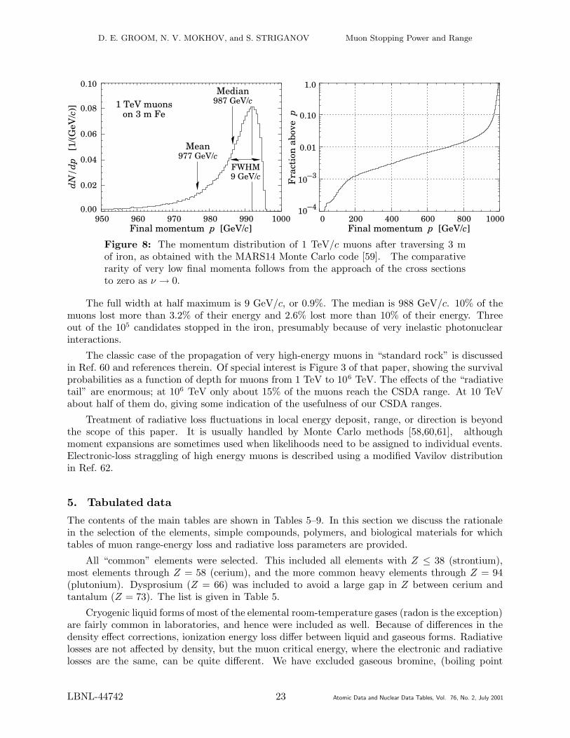
An example illustrating the fluctuations is shown in Fig. 8. The distribution of final muonmomenta was obtained by following 105 1 TeV/c muons through 3 m (2360 g/cm2) of iron, usingthe MARS14 Monte Carlo code [59]. Our result is in nearly exact agreement with results obtainedearlier with TRAMU [58]. The most probable loss is 8 GeV, or 3.4 MeV g−1cm2. Our tables lista stopping power in iron as 9.82 MeV g−1cm2 for a 1 TeV muon, so that the mean loss should be23 GeV, for a final energy (≈ momentum × c) of 977 GeV, far below the peak. This is also themean calculated from the simulated output.



950 960 970 980 990 1000Final momentum p [GeV/c]Final momentum p [GeV/c]

0.00

0.02

0.04

0.06

0.08

0.10

1 TeV muons on 3 m Fe

Mean 977 GeV/c

Median 987 GeV/c

0 200 400 600 800 1000

10–3

10–4

0.01

0.10

1.0dN

/dp

[1/

(GeV

/c)]

Fra

ctio

n ab

ove

p

FWHM 9 GeV/c

Figure 8: The momentum distribution of 1 TeV/c muons after traversing 3 mof iron, as obtained with the MARS14 Monte Carlo code [59]. The comparativerarity of very low final momenta follows from the approach of the cross sectionsto zero as ν → 0.

The full width at half maximum is 9 GeV/c, or 0.9%. The median is 988 GeV/c. 10% of themuons lost more than 3.2% of their energy and 2.6% lost more than 10% of their energy. Threeout of the 105 candidates stopped in the iron, presumably because of very inelastic photonuclearinteractions.

The classic case of the propagation of very high-energy muons in “standard rock” is discussedin Ref. 60 and references therein. Of special interest is Figure 3 of that paper, showing the survivalprobabilities as a function of depth for muons from 1 TeV to 106 TeV. The effects of the “radiativetail” are enormous; at 106 TeV only about 15% of the muons reach the CSDA range. At 10 TeVabout half of them do, giving some indication of the usefulness of our CSDA ranges.

Treatment of radiative loss fluctuations in local energy deposit, range, or direction is beyondthe scope of this paper. It is usually handled by Monte Carlo methods [58,60,61], althoughmoment expansions are sometimes used when likelihoods need to be assigned to individual events.Electronic-loss straggling of high energy muons is described using a modified Vavilov distributionin Ref. 62.

5. Tabulated data

The contents of the main tables are shown in Tables 5–9. In this section we discuss the rationalein the selection of the elements, simple compounds, polymers, and biological materials for whichtables of muon range-energy loss and radiative loss parameters are provided.

All “common” elements were selected. This included all elements with Z ≤ 38 (strontium),most elements through Z = 58 (cerium), and the more common heavy elements through Z = 94(plutonium). Dysprosium (Z = 66) was included to avoid a large gap in Z between cerium andtantalum (Z = 73). The list is given in Table 5.

Cryogenic liquid forms of most of the elemental room-temperature gases (radon is the exception)are fairly common in laboratories, and hence were included as well. Because of differences in thedensity effect corrections, ionization energy loss differ between liquid and gaseous forms. Radiativelosses are not affected by density, but the muon critical energy, where the electronic and radiativelosses are the same, can be quite different. We have excluded gaseous bromine, (boiling point



58.8◦ C, although it is tabulated by Sternheimer et al. [5]. For carbon, two forms with differentdensities appear. In all, 74 range/energy-loss tables are given for 63 elements

We should not overemphasize these differences: Related materials have similar stopping-powerproperties when these are listed in MeV cm2/g (as we do) rather than in MeV/cm. Liquid andgaseous xenon are not dissimilar in spite of a density ratio of 540. Plutonium is more than twice asdense as bismuth, but their stopping powers differ by only 5% at minimum ionization. The stoppingpowers of hydrocarbons are quite similar, as are those of many polymers and biological materials.

Atomic weights are given to the available significance. This varies with element, since theisotopic composition of samples from different sources varies. In general the atomic weights ofelements with only one isotope are known to great precision [63].

The same “commonness” criterion was applied to the selection of the simple compounds listedin Table 6, with some qualifications: We limited ourselves to the compounds listed by Sternheimeret al. [5], which meant that certain common compounds such as NaCl were not available. Commoninorganic scintillators (BaF2, BGO, CsI, LiF, LiI, NaI) are present. Materials such as trichloroethy-lene are included because of their role in important physics experiments. The list contains perhapsmore hydrocarbons than necessary, in part to show the change of stopping power behavior as theH/C ratio changes (note the difference between acetylene and ethane). Liquid water and steam areboth listed. Dry ice was included with some difficulty.

Polymers are listed in Table 7. Their energy loss behavior is quite similar except in the case ofTeflon, which contains no hydrogen. “Thin film” polymers (Mylar, Kapton) were omitted. Polymersused for plastic scintillators (acrylic, polystyrene, polyvinyltolulene) are included. In some casesthe name, like acrylic or polycarbonate, describes a family of polymers. The chemistry given istypical, and no great variation is to be expected except perhaps for “Bakelite,” which is not verywell characterized. Where space permits, the formula is given in such a way as to convey as muchstructural information as possible.

Mixtures of interest are given in Table 8. Muon energy loss in air is of great current interest,given atmospheric neutrino observations. Photographic emulsion is of more historic interest. Exceptfor dry air (and, by definition, standard rock) none of the materials is particularly well characterized.The somewhat arbitrary concrete recipe is taken from The Reactor Handbook [64], and may befound, along with the other compositions, in Ref. 26.

For at least two generations, the depth of underground muon experiments has been reducedto depth in “standard rock.” This is by definition the overburden of the Cayuga Rock Salt Minenear Ithaca, New York, where K. Greisen and collaborators made seminal observations of muons atsubstantial depths [1]. Ref. 1 says only “Most of the ground consists of shales of various types, withaverage density 2.65 g/cm2 and average atomic number 11.” Menon and Murthy later extended thedefinition: 〈Z2/A〉 = 5.5, 〈Z/A〉 = 0.5, and and ρ = 2.65 g/cm2 [65]. It was thus not-quite-sodium.Lohmann et al. [4] further assumed the mean excitation energy and density effect parameters werethose of calcium carbonate, with no adjustments for the slight density difference. We use theirdefinition for this most important material.

Sternheimer et al. [5] list 14 biological materials and “phantoms,” mixtures which have nearlyidentical responses to radiation as the biological materials they replace. Omitted materials can beapproximated by those on the list: Brain (ICRP), lung (ICRP), skin (ICRP), testes (ICRP), softtissue (ICRU 4-component), and striated muscle (ICRU) are quite similar to soft tissue (ICRP), asare several included materials such as eye lens (ICRP) and skeletal muscle (ICRP). Compact bone(ICRU) is similar to cortical bone (ICRP).



Table 5: Index of tables for selected chemical elements. Physical states are indicated by“G” for gas, “D” for diatomic gas, “L” for liquid, and “S” for solid. Gases are evaluatedat one atmosphere and 20◦ C. The corresponding cryogenic liquids are evaluated at theirboiling points at one atmosphere, and carbon is evaluated at several typical densities.Atomic weights are given to their experimental significance. Except where noted, densitiesare as given by Sternheimer, Berger, and Seltzer [5].

Element Symbol Z A State ρ 〈−dE/dx〉min Eµc 〈−dE/dx〉 b Notes[g/cm3] [MeV cm2/g] [GeV] & Range

Hydrogen gas H 1 1.00794 D 8.375× 10−5 4.103 3611. I– 1 VI– 1Liquid hydrogen H 1 1.00794 L 7.080× 10−2 4.034 3102. I– 2 VI– 1 1Helium gas He 2 4.002602 G 1.663× 10−4 1.937 2351. I– 3 VI– 2Liquid helium He 2 4.002602 L 0.125 1.936 2020. I– 4 VI– 2 2Lithium Li 3 6.941 S 0.534 1.639 1578. I– 5 VI– 3Beryllium Be 4 9.012182 S 1.848 1.595 1328. I– 6 VI– 4Boron B 5 10.811 S 2.370 1.623 1169. I– 7 VI– 5Carbon (compact) C 6 12.0107 S 2.265 1.745 1056. I– 8 VI– 6Carbon (graphite) C 6 12.0107 S 1.700 1.753 1065. I– 9 VI– 6Nitrogen gas N 7 14.00674 D 1.165× 10−3 1.825 1153. I–10 VI– 7Liquid nitrogen N 7 14.00674 L 0.807 1.813 982. I–11 VI– 7 2Oxygen gas O 8 15.9994 D 1.332× 10−3 1.801 1050. I–12 VI– 8Liquid oxygen O 8 15.9994 L 1.141 1.788 890. I–13 VI– 8 2Fluorine gas F 9 18.9984032 D 1.580× 10−3 1.676 959. I–14 VI– 9Liquid fluorine F 9 18.9984032 L 1.507 1.634 810. I–15 VI– 9 2Neon gas Ne 10 20.1797 G 8.385× 10−4 1.724 906. I–16 VI–10Liquid neon Ne 10 20.1797 L 1.204 1.695 759. I–17 VI–10 2Sodium Na 11 22.989770 S 0.971 1.639 711. I–18 VI–11Magnesium Mg 12 24.3050 S 1.740 1.674 658. I–19 VI–12Aluminum Al 13 26.981538 S 2.699 1.615 612. I–20 VI–13Silicon Si 14 28.0855 S 2.329 1.664 581. I–21 VI–14 1Phosphorus P 15 30.973761 S 2.200 1.613 551. I–22 VI–15Sulfur S 16 32.066 S 2.000 1.652 526. I–23 VI–16Chlorine gas Cl 17 35.4527 D 2.995× 10−3 1.630 591. I–24 VI–17Liquid chlorine Cl 17 35.4527 L 1.574 1.608 504. I–25 VI–17 2Argon gas Ar 18 39.948 G 1.662× 10−3 1.519 571. I–26 VI–18Liquid argon Ar 18 39.948 L 1.396 1.508 483. I–27 VI–18 2Potassium K 19 39.0983 S 0.862 1.623 470. I–28 VI–19Calcium Ca 20 40.078 S 1.550 1.655 445. I–29 VI–20Scandium Sc 21 44.955910 S 2.989 1.522 420. I–30 VI–21Titanium Ti 22 47.867 S 4.540 1.477 401. I–31 VI–22Vanadium V 23 50.9415 S 6.110 1.436 383. I–32 VI–23Chromium Cr 24 51.9961 S 7.180 1.456 369. I–33 VI–24Manganese Mn 25 54.938049 S 7.440 1.428 357. I–34 VI–25Iron Fe 26 55.845 S 7.874 1.451 345. I–35 VI–26Cobalt Co 27 58.933200 S 8.900 1.419 334. I–36 VI–27Nickel Ni 28 58.6934 S 8.902 1.468 324. I–37 VI–28Copper Cu 29 63.546 S 8.960 1.403 315. I–38 VI–29Zinc Zn 30 65.39 S 7.133 1.411 308. I–39 VI–30Gallium Ga 31 69.723 S 5.904 1.379 302. I–40 VI–31Germanium Ge 32 72.61 S 5.323 1.370 295. I–41 VI–32



Table 5: continued

Element Symbol Z A State ρ 〈−dE/dx〉min Eµc 〈−dE/dx〉 b Notes[g/cm3] [MeV cm2/g] [GeV] & Range

Arsenic As 33 74.92160 S 5.730 1.370 287. I–42 VI–33Selenium Se 34 78.96 S 4.500 1.343 282. I–43 VI–34Bromine Br 35 79.904 L 3.103 1.385 278. I–44 VI–35 2Krypton gas Kr 36 83.80 G 3.478× 10−3 1.357 321. I–45 VI–36Liquid krypton Kr 36 83.80 L 2.418 1.357 274. I–46 VI–36 2Rubidium Rb 37 85.4678 S 1.532 1.356 271. I–47 VI–37Strontium Sr 38 87.62 S 2.540 1.353 262. I–48 VI–38Zirconium Zr 40 91.224 S 6.506 1.349 244. I–49 VI–39Niobium Nb 41 92.90638 S 8.570 1.343 237. I–50 VI–40Molybdenum Mo 42 95.94 S 10.220 1.330 232. I–51 VI–41Palladium Pd 46 106.42 S 12.020 1.289 214. I–52 VI–42Silver Ag 47 107.8682 S 10.500 1.299 211. I–53 VI–43Cadmium Cd 48 112.411 S 8.650 1.277 208. I–54 VI–44Indium In 49 114.818 S 7.310 1.278 206. I–55 VI–45Tin Sn 50 118.710 S 7.310 1.263 202. I–56 VI–46Antimony Sb 51 121.760 S 6.691 1.259 200. I–57 VI–47Iodine I 53 126.90447 S 4.930 1.263 195. I–58 VI–48Xenon gas Xe 54 131.29 G 5.485× 10−3 1.255 226. I–59 VI–49Liquid xenon Xe 54 131.29 L 2.953 1.255 195. I–60 VI–49 2Cesium Cs 55 132.90545 S 1.873 1.254 195. I–61 VI–50Barium Ba 56 137.327 S 3.500 1.231 189. I–62 VI–51Cerium Ce 58 140.116 S 6.657 1.234 180. I–63 VI–52Dysprosium Dy 66 162.50 S 8.550 1.175 161. I–64 VI–53Tantalum Ta 73 180.9479 S 16.654 1.149 145. I–65 VI–54Tungsten W 74 183.84 S 19.300 1.145 143. I–66 VI–55Platinum Pt 78 195.078 S 21.450 1.128 137. I–67 VI–56Gold Au 79 196.96655 S 19.320 1.134 136. I–68 VI–57Mercury Hg 80 200.59 L 13.546 1.130 136. I–69 VI–58Lead Pb 82 207.2 S 11.350 1.122 134. I–70 VI–59Bismuth Bi 83 208.98038 S 9.747 1.128 133. I–71 VI–60Thorium Th 90 232.0381 S 11.720 1.098 124. I–72 VI–61Uranium U 92 238.0289 S 18.950 1.081 120. I–73 VI–62Plutonium Pu 94 244.064197 S 19.840 1.071 117. I–74 VI–63

Notes:

1. Density effect parameters adjusted to this density using Eq. (A.8).

2. Density effect parameters calculated via the Sternheimer-Peierls algorithm discussed in Appendix A.



Table 6: Index of tables for selected simple compounds. Physical states are indicated by“G” for gas, “D” for diatomic gas, “L” for liquid, and “S” for solid. Gases are evaluatedat one atmosphere and 20◦ C. Except where noted, densities are those given by Stern-heimer, Berger, and Seltzer [5]. Composition not explained may be found in Seltzer andBerger [26] or in the file properties.datat http://pdg.lbl.gov/AtomicNuclearProperties.

Compound or mixture 〈Z/A〉 State ρ 〈−dE/dx〉min Eµc 〈−dE/dx〉 b Notes[g/cm3] [MeV cm2/g] [GeV] & Range

Acetone (CH3CHCH3) 0.55097 L 0.790 2.003 1160. II– 1 VII– 1Acetylene (C2H2) 0.53768 G 1.097× 10−3 2.025 1400. II– 2 VII– 2Aluminum oxide (Al2O3) 0.49038 S 3.970 1.647 705. II– 3 VII– 3Barium fluoride (BaF2) 0.42207 S 4.890 1.303 227. II– 4 VII– 4Beryllium oxide (BeO) 0.47979 S 3.010 1.665 975. II– 5 VII– 5Bismuth germanate (BGO, Bi4(GeO4)3) 0.42065 S 7.130 1.251 176. II– 6 VII– 6Butane (C4H10) 0.59497 G 2.493× 10−3 2.278 1557. II– 7 VII– 7Calcium carbonate (CaCO3) 0.49955 S 2.800 1.686 630. II– 8 VII– 8Calcium fluoride CaF2 0.49670 S 3.180 1.655 564. II– 9 VII– 9Calcium oxide (CaO) 0.49929 S 3.300 1.650 506. II–10 VII–10Carbon dioxide (CO2) 0.49989 G 1.842× 10−3 1.819 1094. II–11 VII–11Solid carbon dioxide (dry ice) 0.49989 S 1.563 1.787 927. II–12 VII–11 2Cesium iodide (CsI) 0.41569 S 4.510 1.243 193. II–13 VII–12Diethyl ether ((CH3CH2)2O) 0.56663 L 0.714 2.072 1220. II–14 VII–13Ethane (C2H6) 0.59861 G 1.253× 10−3 2.304 1603. II–15 VII–14Ethanol (C2H5OH) 0.56437 L 0.789 2.054 1178. II–16 VII–15Lithium fluoride (LiF) 0.46262 S 2.635 1.614 903. II–17 VII–16Lithium iodide (LiI) 0.41939 S 3.494 1.272 207. II–18 VII–17Methane (CH4) 0.62334 G 6.672× 10−4 2.417 1715. II–19 VII–18Octane (C8H18) 0.57778 L 0.703 2.123 1312. II–20 VII–19Paraffin (CH3(CH2)n≈23CH3) 0.57275 S 0.930 2.088 1287. II–21 VII–20Plutonium dioxide (PuO2) 0.40583 S 11.460 1.158 136. II–22 VII–21Liquid propane (C3H8) 0.58962 L 0.493 2.198 1365. II–23 VII–22 1Silicon dioxide (fused quartz, SiO2) 0.49930 S 2.200 1.699 708. II–24 VII–23 1Sodium iodide (NaI) 0.42697 S 3.667 1.305 223. II–25 VII–24Toluene (C6H5CH3) 0.54265 L 0.867 1.972 1203. II–26 VII–25Trichloroethylene (C2HCl3) 0.48710 L 1.460 1.656 568. II–27 VII–26Water (liquid) (H2O) 0.55509 L 1.000 1.992 1032. II–28 VII–27Water (vapor) (H2O) 0.55509 G 7.562× 10−4 2.052 1231. II–29 VII–27

Notes:

1. Density effect parameters adjusted to this density using Eq. (A.8). Ref. 5 lists 2.32 g/cm3 for SiO2,which may be the density of cristobalite. The density of crystalline quartz is about 2.65 g/cm3, and thedensity of fused quartz is typically 2.20 g/cm3.

2. Density effect parameters calculated via the Sternheimer-Peierls algorithm discussed in Appendix A.



Table 7: Index of tables for selected high polymers. Except where noted, densities arethose given by Sternheimer, Berger, and Seltzer [5]; actual densities of polymers willvary. Composition not explained may be found in Seltzer and Berger [26] or in the fileproperties.dat at http://pdg.lbl.gov/AtomicNuclearProperties.

Compound or mixture 〈Z/A〉 ρ 〈−dE/dx〉min Eµc 〈−dE/dx〉 b Notes[g/cm3] [MeV cm2/g] [GeV] & Range

Bakelite [C43H38O7]n 0.52792 1.250 1.889 1110. III– 1 VIII– 1Nylon (type 6, 6/6) [C12H22O2N2]n 0.54790 1.180 1.973 1156. III– 2 VIII– 2 1Polycarbonate [OC6H4C(CH3)2C6H4OCO]n 0.52697 1.200 1.886 1104. III– 3 VIII– 3Polyethylene [C2H4]n 0.57034 0.890 2.079 1282. III– 4 VIII– 4 1Polymethylmethacrylate (acrylic) 0.53937 1.190 1.929 1107. III– 5 VIII– 5Polystyrene [C6H5CHCH2]n 0.53768 1.060 1.936 1183. III– 6 VIII– 6Polytetrafluoroethylene (Teflon) [C2F4]n 0.47992 2.200 1.671 853. III– 7 VIII– 7Polyvinylchloride (PVC) [CH2CHCl]n 0.51201 1.300 1.779 696. III– 8 VIII– 8Polyvinyltoluene [2-CH3C6H4CHCH2]n 0.54141 1.032 1.956 1194. III– 9 VIII– 9

Notes:

1. Density effect parameters adjusted to this density using Eq. (A.8).

Table 8: Index of tables for selected mixtures. Physical states are indicated by “G” forgas and “S” for solid. Gases are evaluated at one atmosphere and 20◦ C. Densities arethose given by Sternheimer, Berger, and Seltzer [5]. Composition may be found in Seltzerand Berger [26] or in the file properties.dat athttp://pdg.lbl.gov/AtomicNuclearProperties.

Compound or mixture 〈Z/A〉 State ρ 〈−dE/dx〉min Eµc 〈−dE/dx〉 b[g/cm3] [MeV cm2/g] [GeV] & Range

Air (dry, 1 atm) 0.49919 G 1.205× 10−3 1.815 1114. IV– 1 IX– 1Concrete 0.50274 S 2.300 1.711 700. IV– 2 IX– 2Lead glass 0.42101 S 6.220 1.255 175. IV– 3 IX– 3Photographic emulsion 0.43663 S 6.470 1.313 235. IV– 4 IX– 4Plate glass 0.49731 S 2.400 1.684 670. IV– 5 IX– 5Standard rock 0.50000 S 2.650 1.688 693. IV– 6 IX– 6



Table 9: Index of tables for selected biological materials. Physical states are indicatedby “L” for liquid and “S” for solid. Densities are those given by Sternheimer, Berger,and Seltzer [5]. Composition may be found in Seltzer and Berger [26] or in the fileproperties.dat at http://pdg.lbl.gov/AtomicNuclearProperties.

Biological material 〈Z/A〉 State ρ 〈−dE/dx〉min Eµc 〈−dE/dx〉 bor phantom [g/cm3] [MeV cm2/g] [GeV] & Range

A-150 tissue-equivalent plastic 0.54903 S 1.127 1.978 1158. V– 1 X– 1Adipose tissue (ICRP) 0.55947 S 0.920 2.029 1183. V– 2 X– 2Blood (ICRP) 0.54995 L 1.060 1.971 1032. V– 3 X– 3Cortical bone (ICRP) 0.52130 S 1.850 1.803 748. V– 4 X– 4C-552 air-equivalent plastic 0.49969 S 1.760 1.760 953. V– 5 X– 5Eye lens (ICRP) 0.54977 S 1.100 1.971 1057. V– 6 X– 6MS20 tissue substitute 0.53886 S 1.000 1.934 1056. V– 7 X– 7Skeletal muscle (ICRP) 0.54938 S 1.040 1.970 1032. V– 8 X– 8Soft tissue (ICRP) 0.55121 S 1.000 1.982 1063. V– 9 X– 9

Acknowledgments

We wish to thank Felix Boehm (Caltech) for the invitation to write this report, and for his(and the editor’s) gentle reminders and infinite patience while the work was in progress. AlbertoFasso (SLAC) was kind enough to make available his ASCII files of the density-effect coefficientsand composition, vastly aiding verification of our parameters. Steve Seltzer (NIST) answered ourquestions and made available code which produced computer-readable files of the main tables ofICRU 49, making comparisons with our results much easier. Hans Bichsel, our “ghost author,”first provided us with an exhaustive and supportive referee’s report. This led to many changesand additions, including two new figures. Then, via conversations and email, further changes weremade, and his suggested wording was used in parts of Sections 3.1 and 3.3. Finally, Bob Naumann(Dartmouth) carefully checked and corrected our structures for polymers. This work was supportedby the U.S. Department of Energy under contract No. DE-AC03-76SF00098.



Appendix A. Stopping power and density-effect parameters for compounds

and mixtures

For most of the materials for which tables are given in this report, the relevant effective excitationenergy and density-effect parameters have already been tabulated, and should be used. This sectionconcerns how to deal with an untabulated compound or mixture.

It is usual to think of a compound or mixture as made up of thin layers of the pure elements(or, better, constituent compounds for which tabulated data are available) in the right proportion(Bragg additivity [66]) . Let nj be the number of the jth kind of atom in a compound (it need notbe an integer for a mixture), and wj its weight fraction:

wj = njAj

/

∑

k

nkAk A.1

Then⟨

dE

dx

⟩

=∑

j

wj

dE

dx

∣

∣

∣

∣

j

A.2

When the Bethe-Bloch equation is inserted and the radiative terms added, the Z-dependent termscan be sorted out to find that the mixture or compound is equivalent to a single material with

⟨

Z

A

⟩

=∑

j

wj

Zj

Aj

=∑

j

njZj

/

∑

j

njAj

ln 〈I〉 =∑

j

wj (Zj/Aj) ln Ij

/

∑

j

wj (Zj/Aj) =∑

j

njZj ln Ij

/

∑

j

njZj

〈b (E)〉 =∑

j

wjbj (E)

A.3

There are pitfalls in actually using Eq. (A.3) to calculate 〈I〉. Since the electrons in a compoundare more tightly bound than in the constituent elements, the effective Ij are in general higher thanthose of the constituent elements. Exceptions are provided by diatomic gases and by metals inmetallic alloys or compounds. Berger and Seltzer discuss ways to extend the Bragg additivity rulein lieu of a detailed calculation [26]:

(a) For a select list of materials (carbon and some common gases), they propose alternate meanexcitation energies in their Table 5.1 (or Table 6 in Ref. 26).

(b) For other elements, the excitation energies are multiplied by 1.13 before calculation of the mean(the “13% rule”). Although it is is not said, it would seem sensible to apply this rule in the caseof a tightly-bound material such as CsI, and not apply it in the case of a metallic compoundlike Nb3Sn.

(c) Both are superseded by experimental numbers when available, as in the case of SiO2.

Bragg additivity has little meaning in calculating the density-effect correction. If the materialof interest is not available in the tables of Ref. 5, then the algorithm given by Sternheimer andPeierls [6] should be used. Their recipe is given more succinctly in the EGS4 manual [28], and thefollowing algorithm is adopted from that version for the parameterization of Section 3.4.

(a) I is obtained as described above

(b) k is always taken as 3.00

(c) C = 2 ln(I/hωp) + 1, with the plasma energy hωp obtained using the expression from Table 1.



(d) For solids and liquids,

x1 =

2.0 if I < 100 eV, and x0 =

{

0.2 if C < 3.6810.326C − 1.0 otherwise

3.0 if I ≥ 100 eV, and x0 =

{

0.2 if C < 5.2150.326C − 1.5 otherwise

A.4

(e) In the case of gases,

x0 =

1.6 and x1 = 4.0 if C < 10.01.7 and x1 = 4.0 if 10.0 ≤ C < 10.51.8 and x1 = 4.0 if 10.5 ≤ C < 11.01.9 and x1 = 4.0 if 11.0 ≤ C < 11.52.0 and x1 = 4.0 if 11.5 ≤ C < 12.252.0 and x1 = 5.0 if 12.25 ≤ C < 13.8040.326C − 1.5

and x1 = 5.0 if C ≥ 13.804

A.5

(f)

a =C − 2 (ln 10) x0

(x1 − x0)3 . A.6

We have used this algorithm to calculate the density-effect coefficients for cryogenic liquids,which are not tabulated by Sternheimer, Berger, and Seltzer [5]. In this case, I for the gas was used.

One problem remains: Given the density-effect parameters, either from the literature [5] orfrom the algorithm given above, how does one modify them for the same material at a differentdensity? This problem occurs for gases at different pressures, or for solid and liquids at differentdensities than those tabulated. In an early paper [6], Sternheimer noted that under quite generalconditions

δr (p) = δ(

p√

r)

, A.7

where r = ρ/ρ0, the ratio of desired to tabulated densities, and the subscript r indicates the quantityevaluated at the desired density. This implies [6] that

Cr = C − ln r

x0r = x0 − 12log10 r

x1r = x1 − 12log10 r .

A.8

It is easily shown by matching different regions in Eq. (11) that the parameters a and k areunchanged by the transformation.

This method was used to correct the parameters for several materials for which we preferdifferent densities, for example the density of fused silica. Liquid hydrogen is tabulated for the“bubble chamber density,” for which we scaled the parameters to the density of liquid hydrogen atits boiling point at a pressure of one atmosphere.

Both algorithms were checked by calculating 〈−dE/dx〉 several ways, taking advantage of thefact that Ref. 5 lists both gaseous and liquid helium, three densities of carbon, and both steam andliquid water. The comparisons are discussed at the end of Sect. 3.4.



Appendix B. Direct pair production from screened nuclei

Nikishov’s analytic form for the cross section is given by [50]

dσ

dν

∣

∣

∣

∣

pair, nucl

=(2αreZ)

2

π

(1 − ν)

ν

[

(f1 + θf3) ln

(

2ε

me

)

+ φ2 + θφ4 + I

]

, B.1

where ε = νE is the energy transferred to the e+e− pair, and θ = m2e/M

2. The functions in thesquare brackets are given by

f1 + θf3 =44

45z− 16

45− 4

9θ −

(

7

9+

8

45z +

7

18zθ

)

ln z

+

[

16

45z +

38

45− 44

45z+

4

3 (z + 4)+

(

7

9z − 2

9+

8

3 (z + 4)

)

θ

]

B (z) lnz2

z1

,B.2

φ2 + θφ4 =

(

7

36+

2

45z +

7

72zθ

)(

ln2 z2

z1

+ π2 + 2 ln2 z

)

+

(

7

18+

3

20z +

7

36zθ

)

ln z +653

270− 28

9z+

2

3θ

+

[

− 3

10z − 92

45+

52

45z−(

2

9− 7

18z

)

θ

]

B (z) lnz2

z1

+ B (z)

[

− 8

45z − 19

45− 8

45z−(

2

9+

7

18z

)

θ

] [

Li2 (y) + 2Li2

(

1

z2

)

+3

2ln2 z2

z1

]

+

(

8

z+ zθ

)

B (z)

3 (z + 4)×[

6Li2

(

1

z2

)

− Li2 (y) +1

2ln2 z2

z1

]

,

B.3

where

z =ν2

θ (1 − ν), z1,2 = B (z) ∓ 1

2, B (z) =

√

1

4+

1

z, y =

z1 + z2

z22

,

Li2 is the dilogarithm function (Spence’s integral evaluated for n = 2) [67], and

I =

(

7

9+

8

45z +

7

18zθ

)

H −[

16

45z +

38

45+

16

45z+

(

7

9z +

4

9

)

θ

]

B (z) J+

+

[

−16

45z − 14

9− 8

9w+

2

45

z

w− 4

5

z

w2+

2z

3 (w + 4)−(

7

9z +

4

9

z

w

)

θ

]

B (w) I+

+

[

32

45

u

w− 88

45z− 16

45w+

8

5

z

w2+

8

9

u

wθ

]

B (u) lnu2

u1

+

[

68

45− 16

45z+

8

3w− 2

3

z

w− 8

9θ

]

B (z) lnz2

z1

+104

45z

− 8

15w− 62

27−(

8

9w+

1

45

z

w+

4

5

z

w2+

4

9

z

wθ

)

ln z

+

(

1 +1

2zθ

)

1

3w

(

ln2 u2

u1

− ln2 z2

z1

)

+

(

8

z+ zθ

)

B (z)

3 (z + 4)−[

2J(2)+ + ln2 z2 − ln2 z1

]

,

B.4

where

w = s√

z, s =2√

γγ′Z1/3

183√

e≈

√γγ′Z1/3

151,

u = w + z, γ = P0/M, γ′ = P ′

0/M

B.5



(u1,2, B(u) and w1,2, B(w) are the analogs of z1,2, B(z), i. e., u1,2 = B(u) ∓ 12, etc.),

H = Li2

(

z

u + 4

)

− Li2

(

z + 4

u + 4

)

+ Li2

(

z

z + 4

)

− 2Li2

(

u

u + 4

)

+ Li2

(

4w

u (z + 4)

)

+ Li2

(

4z

u (w + 4)

)

− Li2

(

4

w + 4

)

+π2

6

+ 2 ln (z1) ln (z2) − 4 ln (u1) ln (u2) − ln2 z + ln2 (z + 4) − ln

(

1 +4

w

)

ln (u + 4)

− ln (4w) ln (z + 4) + ln (16) ln (u + 4) − ln2 (u + 4) + 2 ln2 u

+ ln (u) ln

(

z + 4

4

w + 4

4w

)

− ln (z) ln

(

z + 4

4

u

w

)

, J+ = J(1)+ + J

(2)+ ,

B.6

J (1)+ = 2Li2

(

1

z2

)

− Li2 (y) + ln (z1) lnz2

z1

, y =z1 + z2

z22

, B.7

J(2)+ = Li2

(

u1

z1

)

− Li2

(

u2

z2

)

+ Li2

(

z1

z1 + u2

)

− Li2

(

z2

z2 + u1

)

+ ln

(

u1

z1

)

ln

(

1 − u1

z1

)

− ln

(

u2

z2

)

ln

(

1 − u2

z2

)

+ ln

(

z2

zi

)

ln [u (z1 + u2)] ,

B.8

and, finally,

I+ = Li2

(

u1

w1

)

− Li2

(

u2

w2

)

− 2Li2

(

w1

w2

)

+ Li2

(

w1

w1 + u2

)

− Li2

(

w2

w2 + u1

)

+π2

3+ ln

(

w2

w1

)

ln

(

w1 + u2

w2

u

z

)

+ ln

(

u1

w1

)

ln

(

1 − u1

w1

)

− ln

(

u2

w2

)

ln

(

1 − u2

w2

)

.

B.9



References

1. P. H. Barrett, L. M. Bollinger, G. Cocconi, Y. Eisenberg, and K. Greisen, Rev. Mod. Phys.24, 133 (1952).

2. R. M. Sternheimer, Phys. Rev. 117, 485 (1960) 983–991 (1994).

3. “Stopping Powers and Ranges for Protons and Alpha Particles,” ICRU Report No. 49 (1993);

Tables and graphs of these data are available at http://physics.nist.gov/PhysRefData/.

4. W. Lohmann, R. Kopp, and R. Voss, “Energy Loss of Muons in the Energy Range 1–10000 GeV,”CERN Report 85–03 (1985).

5. R. M. Sternheimer, M. J. Berger, and S. M. Seltzer, Atomic Data and Nuclear Data Tables30, 261–271 (1984).

6. R. M. Sternheimer and R. F. Peierls, Phys. Rev. B3, 3681–3692 (1971).

7. P. J. Mohr and B. N. Taylor, “CODATA Recommended Values of the Fundamental PhysicalConstants: 1998,” J. Phys. Chem. Ref. Data 28, 1713–1852 (1999).

8. W. H. Barkas, W. Birnbaum, and F. M. Smith, Phys. Rev. 101, 778 (1956);

H. Bichsel, Phys. Rev. A41, 3642–3647 (1990).

9. E. Fermi and E. Teller, Phys. Rev. 72, 399–408 (1947).

10. J. Lindhard, Kgl. Danske Videnskab. Selskab, Mat.-Fys. Medd. 28, No. 8 (1954);

J. Lindhard, M. Scharff, and H. E. Schiøtt, Kgl. Danske Videnskab. Selskab, Mat.-Fys.Medd. 33, No. 14 (1963).

11. T. Kaneko, Atomic Data and Nuclear Data Tables 53, 271–283 (1993).

12. H. H. Andersen and J. F. Ziegler, Hydrogen: Stopping Powers and Ranges in All Elements.

Vol. 3 of The Stopping and Ranges of Ions in Matter (Pergamon Press, 1977).

13. H. A. Bethe, “Quantenmechanic der Ein- und Zwei-Elektronen Probleme,’ Handbuch der

Physik, Vol. 24/1 (Springer-Berlin, 1933), p. 273.

14. S. R. Kelner, R. P. Kokoulin and A. A. Petrukhin, Phys. Atomic Nuclei 60, 576–583 (1997)(Yad. Fiz. 60, 657 (1997)).

15. J. D. Jackson, Phys. Rev. D59, 017301 (1999).

16. M. S. Livingston and H. A. Bethe, Rev. Mod. Phys. 9 245–390 (1937); see especially pp. 261–276.

17. B. Rossi, High Energy Particles, (Prentice-Hall, Inc., Englewood Cliffs, NJ, 1952).

18. E. A. Uehling, Ann. Rev. Nucl. Sci. 4, 315 (1954).

19. U. Fano, Ann. Rev. Nucl. Sci. 13, 1 (1963).

20. M. Inokuti, Rev. Mod. Phys. 43, 297 (1971).

21. H. Bichsel, in American Institute of Phyics Handbook, 3rd ed., edited by E. D. Gray (McGraw-Hill, New York, 1972), section 8d.

22. J. D. Jackson, Classical Electrodynamics, 2nd ed. (John Wiley & Sons, New York, 1975).

23. S. P Ahlen, Rev. Mod. Phys. 52, 121 (1980).



24. H. Bichsel, in Atomic, Molecular, and Optical Physics Handbook, edited by G. Drake, (Am.Inst. Phys., 1996), Chap. 87.

25. H. Bethe, Ann. Phys. 5, 325 (1930).

26. S. M. Seltzer and M. J. Berger, Int. J. Appl. Radiat. 33, 1189–1218 (1982).

27. ICRU Report 37, “Stopping Powers for Electrons and Positrons,” International Commissionon Radiation Units and Measurements, Washington, DC (1984);

Tables and graphs of these data are available at http://physics.nist.gov/PhysRefData/.

28. W.R. Nelson, H. Hirayama, and D. W. O. Rogers, “The EGS4 Code System,” SLAC-265,Stanford Linear Accelerator Center (Dec. 1985).

29. H. Bichsel, Phys. Rev. A46, 5761 (1992).

30. W. H. Barkas and M. J. Berger, “Tables of Energy Losses and Ranges of Heavy ChargedParticles,” in Studies in Penetration of Charged Particles in Matter, National Academy ofSciences–National Research Council, Publication 1133 (1964), p. 103.

31. T. Hiraoka et al., Phys. Med. Biol. 39, 983–991 (1994).

32. P. T. Leung, Phys. Rev. A40, 5417 (1989) 983–991 (1994).

33. W. H. Barkas, N. J. Dyer, and H. H. Heckmann, Phys. Rev. Lett. 11, 26 (1963).

34. M. Agnello et al., Phys. Rev. Lett. 74, 371 (1995).

35. R. M. Sternheimer, Phys. Rev. 88, 851 (1952).

36. R. M. Sternheimer, S. M. Seltzer, and M. J. Berger, Phys. Rev. B26, 6067–6076 (1982).

37. S. M. Seltzer and M. J. Berger, Int. J. Appl. Radiat. 35, 665–676 (1984). This paper correctsand extends the results of [26].

38. H. Bichsel, Rev. Mod. Phys. 60, 663 (1960).

39. S. M. Seltzer, private communication.

40. J. D. Jackson and R. L. McCarthy, Phys. Rev. B6, 4131 (1972).

41. H. A. Bethe and W. Heitler, Proc. Roy. Soc. A146, 83 (1934);

R. M. Sternheimer, S. M. Seltzer, and M. J. Berger, Phys. Rev. B27, 6971 (1983) (erratum).

42. A. V. Petrukhin and V. V. Shestakov, Can. J. Phys. 46, S337 (1968).

43. W. K. Sakumoto et al., Phys. Rev. D45, 3042 (1992).

44. S. R. Kelner, R. P. Kokoulin and A. A. Petrukhin, preprint MSEPI 024-95, Moscow (1995),available as CERN Preprint Server SCAN-9510048.

45. Y. M. Andreev and E. V. Bugaev, Phys. Rev. D55, 1233 (1997).

46. S. R. Kelner, R. P. Kokoulin and A. A. Petrukhin, Phys. Atomic Nuclei 62, 1894–1898 (1999).

47. G. Racah, Nuovo Cim. 16, 93 (1937).

48. S. R. Kelner and Yu. D. Kotov, Sov. Jour. Nucl. Phys. 7, 237 (1968) (Yad. Phys. 7, 360(1968)).

49. R. P. Kokoulin and A. A. Petrukhin, Acta Physica Acad. Sci. Hung. 29 Suppl. 4, 277 (1970).

50. A. I. Nikishov, Sov. J. Nucl. Phys. 27, 677–691 (1978) ((Yad. Phys. 27, 1281–1289 (1978)).



51. S. R. Kelner, Phys. Atomic Nuclei 61, 448 (1998) (Yad. Phys. 61, 511 (1998)).

52. L. B. Bezrukov and E. V. Bugaev, Sov. J. Nucl. Phys. 33 635–643 (1981) (Yad. Phys. 33,1195–1207 (1981)).

53. E. Scapparone et al., Nucl. Phys. B, Proc. Suppl. 75A, 397–400 (1999).

54. T. A. Armstrong et al., Phys. Rev. D5, 1640 (1972);

T. A. Armstrong et al., Nucl. Phys. B41, 445 (1972).

55. C. Caso et al., “Review of Particle Physics,” Eur. Phys. J. C3, 1 (1998);

The values calculated in this paper are used in the 2000 revision of the Gaisser and Stanevreview in D. E. Groom et al., “Review of Particle Physics,” Eur. Phys. J. C15, 1 (2000);

See also http://pdg.lbl.gov.

56. E. Berger et al., Z. Phys. C73, 455–463(1997).

57. I. L. Rozental Sov. Phys. Uspekhi 11, 49 (1968) (Usp. Phys. Nauk. 94, 91 (1968)).

58. A. Van Ginneken, Nucl. Instrum. Methods A251, 21–39 (1986).

59. N.V. Mokhov, “The MARS Code System User’s Guide,” Fermilab-FN-628 (1995);

N. V. Mokhov, S. I. Striganov, A. Van Ginneken, S. G. Mashnik, A. J. Sierk, J.Ranft, inProc. of the Fourth Workshop on Simulating Accelerator Radiation Environments (SARE-4), Knoxville, TN, September 14-16, 1998, pp. 87–99, Fermilab-Conf-98/379 (1998), nucl-th/9812038-v2-16-Dec-1998;

N. V. Mokhov, in Proc. of ICRS-9 International Conference on Radiation Shielding, (Tsukuba,Ibaraki, Japan, 1999), J. Nucl. Sci. Tech., 1 (2000), pp. 167–171, Fermilab-Conf-00/066 (2000);

http://www-ap.fnal.gov/MARS/.

60. P. Lipari and T. Stanev, Phys. Rev. D44, 3543 (1991).

61. S. I. Striganov, Nucl. Phys. B (Proc. Suppl.) 51A, 172 (1996).

62. S. I. Striganov, Nucl. Instrum. Methods A322, 225–230 (1992).

63. Commission on Atomic Weights and Isotopic Abundances, Pure and Appl. Chem. 68, 2339(1996);

G. Audi and A. H. Wapstra, Nucl. Phys. A565, 1 (1993).

64. The Reactor Handbook, 2nd ed. edited by R. C. Weast, (Interscience, New York, 1960), Vol. 1.

65. M. G. K. Menon and P. V. Ramana Murthy, in Progress In Elementary Particle and Cosmic

Ray Physics, (North Holland, Amsterdam, 1967), Vol. 9, 161–243.

66. W. H. Bragg and R. Kleeman, Philos. Mag. 10, 318 (1905).

67. M. Abramowitz and I. A. Stegun, Handbook of Mathematical Functions, National Bureauof Standards Applied Mathematics Series, No. 55, (U. S. Gov. Printing Office, 1964). Thedilogarithm (Spence’s integral for n = 2) is given by Eq. 27.7.1. CERNLIB routine DDILOGis used to calculate the function.



Explanation of Tables4

TABLE I: Muon energy loss rate and CSDA range for selected chemical elements.

The contents of Table I and other information are given in Table 5.

The header defines the element and state, and gives the parameters used to calculatethe electronic stopping power:

Z: Atomic number.

A: Atomic weight.

ρ: Density. Gas density is evaluated at 20◦ C.

I: Mean excitation energy.

a—δ0: Sternheimer et al. density effect parameters, as introduced in Sect. 3.4 and Eq. (11).

The body of the table presents ionizing energy loss (Eq. (15)) and the componentsof radiative loss rate (see Eqs. (1) and (2), as well as CSDA range obtained byintegrating the total (Eq. (3)), as a function of the muon’s initial kinetic energy T .The spacing of the independent variable is fairly uniform on a logarithmic scale.The corresponding momentum p is also given. The table is interrupted to show thepoints at which minimum ionization and muon critical energy (Eq. (5)) occur.

A radiative loss field is left blank if the stopping power contribution is less than 0.0001.

TABLE II: Muon energy loss rate and CSDA range for simple compounds.

The contents of TABLE II and other information are given in Table 6. The formatis identical with TABLE I, except that 〈Z/A〉 (Eq. (A.3)) replaces Z and A.

TABLE III: Muon energy loss rate and CSDA range for high polymers.

The contents of TABLE III and other information are given in Table 7. The formatis identical with TABLE II.

TABLE IV: Muon energy loss rate and CSDA range for mixtures.

The contents of TABLE IV and other information are given in Table 8. The formatis identical with TABLE II.

TABLE V: Muon energy loss rate and CSDA range for biological compounds.

The contents of TABLE V and other information are given in Table 9. The formatis identical with TABLE I, except that 〈Z/A〉 (Eq. (A.3))) replaces Z and A.

TABLE VI: b values for the elements listed in Table I.

Interpolation in log E is used to generate the b values shown in TABLE I and forthe ionizing loss calculations. The contents are listed in Table 5.

TABLE VII: b values for the compounds listed in TABLE II.

TABLE VII has the same format as TABLE III except that 〈Z/A〉 replaces Z and A.The contents are listed in Table 6.

TABLE VIII: b values for the high polymers listed in TABLE III.

TABLE VII has the same format as TABLE VII. The contents are listed in Table 7.

TABLE IX: b values for the mixtures listed in TABLE IV.


TABLE X: b values for the biological compounds listed in TABLE V.


4 Computer-readable versions of these tables can be found at http://pdg.lbl.gov/AtomicNuclearProperties


Documents

MUON STOPPING POWER AND RANGE TABLES 10 …pdg.lbl.gov/2017/AtomicNuclearProperties/adndt.pdf · MUON STOPPING POWER AND RANGE TABLES 10 MeV|100 TeV DONALD E. GROOM ... Density e