MPRAMunich Personal RePEc Archive

Oil price shocks, poverty, and gender: asocial accouting matrix analysis forKenya

Jean-Pascal Nganou and Juan Carlos Parra and Quentin

Wodon

World Bank

2009

Online at https://mpra.ub.uni-muenchen.de/28471/MPRA Paper No. 28471, posted 31. January 2011 00:12 UTC

Oil Price Shocks, Poverty, and Gender: A Social Accounting Matrix Analysis for Kenya

Jean-Pascal Nganou, Juan Carlos Parra, and Quentin Wodon†

Following pioneering work by Stone (1985), among others, social accounting matrices (SAMs) have been used as consistent accounting frameworks reconciling national income and product accounts with input-output analysis and in many cases household survey data. A SAM is primarily a data framework, but it can also be used as a model. As a database, a SAM is a double-entry square matrix recording in columns payments (or expenditures) and in rows receipts (or incomes) of transactions made by various activities, commodities, and agents in the economy. SAMs are constructed according to the same accounting principles underlying input-output tables (that is, each operation is recorded twice, so that any inflow into one account must be balanced by an outflow from a counterpart account). When SAMs are used as models—to assess the impact of trade shocks, for example—they are typically static models with fixed technical coefficients (that is, Leontief technology) and prices (as explained below). The key advantage of SAMs over input-output tables for distributional analysis is that the data from household surveys on the incomes and consumption patterns of various types of households can be directly integrated into the modeling exercise in order to conduct distributional analysis.

Most of the applications of the SAM technique have focused on the impact of exogenous quantity or demand shocks (a brief review of the literature is provided later in this paper). The objective here is instead to use a recent SAM for Kenya to assess the potential impact of the increase in oil prices on the cost of the consumption basket of various types of households.1 Indeed, virtually everything that can be done for quantity shocks using SAMs can also be done for price shocks, as discussed in the next section. The key advantage of the Kenya SAM is that it defines the categories of households by poverty status (ultrapoor, poor, and nonpoor); gender (male or female household head); and location (urban versus rural). This makes it feasible to take into account both poverty and gender dimensions simultaneously in assessing who will suffer most from an increase in oil prices.

The increase in oil prices is important, because many developing countries have had difficulties paying higher oil prices. This has manifested itself most visibly through higher deficits by electric utilities in countries in which a substantial part of power generation is thermal. In some countries taxes on oil products have been reduced in order to limit the impact of rising prices on consumers. But in a majority of countries, pass-throughs are in place, which means that consumers lose purchasing power, both through the higher prices paid for oil-related products and through the more general increase in producer and consumer prices that higher oil prices generate through multiplier effects. It is precisely to be able to take these multiplier effects into account that the use of a SAM model is appropriate.

† Quentin Wodon is the corresponding author; his email address is qwodon@worldbank.org. 1. See Roland-Holst and Sancho (1995) for an application of the SAM price model to the U.S. economy.

2

Work by Semboja (1994) and Karingi and Siriwardana (2003) suggests that the Kenyan economy was already highly vulnerable to oil price shocks in the 1970s (see also Mitra 1994 and Dick and others 1984). Together with Burundi, Rwanda, Tanzania, and Uganda, Kenya belongs to Africa’s Great Lakes region, which borders Lake Kivu, Lake Tanganyika, and Lake Victoria. According to the U.S. Department of Energy’s (2004), Kenya accounted for almost 60 percent of the region’s commercial energy consumption in 2001, despite the fact that its population, at 37 million people, represented only about a third of the 107 million residents of the region. Kenya’s large share in the energy consumption of the region is caused by the fact that the country is richer and more urbanized than its neighbors.

Macroeconomic statistics suggest the potential for a relatively large impact of the increase in oil prices on households and the economy (Kumar 2005). In 2003, for example, net oil imports accounted for 5.6 percent of GDP; this figure rose to 6.9 percent in 2004 and an estimated 8.9 percent in 2005. The incremental cost of oil imports in 2004 over 2003 caused by the increase in prices was about $200 million (1.2 percent of GDP). Inflation was kept in check, but fuel and power prices rose at more than twice the rate of the consumer price index (CPI) between December 2004 and October 2005 (9.2 percent versus 4.4 percent for the CPI). More generally, the substantial impact of the increase in oil prices on the economy is caused by the fact that oil represents an important share of the intermediate inputs of a wide range of sectors, from electricity to transportation. In the case of electricity, while hydroelectric plants account for three-fourths of production, the rest is based in large part on oil. In 2005 the low-cost electricity that had been granted to the Kenya Power and Lighting Company (KPLC) by the Kenya Electricity Generating Company was terminated. According to news stories, the change was motivated by the need to make KPLC more attractive to foreign investors for privatization, but increasing oil prices may have added pressure to increase prices.

This paper is organized as follows. The next section provides a general background on SAMs as a modeling tool (two annexes provide mathematical derivations for the key concepts used). The following section presents the results for Kenya. The last section summarizes the paper’s main conclusions.

Social Accounting Matrices: A Brief Review

For any economic analysis that supposes the existence of general equilibrium feedback effects, a multisectoral approach is typically preferable to a partial equilibrium framework, because interlinkages among different parts of the economy are too complex to be considered in partial equilibrium models.2 In principle, applied general equilibrium analysis can be performed using econometric methods (Jorgenson 1984, 1998) on a system of simultaneous linear or nonlinear equations describing technology and consumption behavior of various sectors and institutions considered. But such an approach requires a considerable amount of data, not readily available for many countries, including industrial economies. To circumvent these data requirements, researchers have used static input-output and SAM–based general equilibrium models in much of the empirical work on developing economies. These models require only a single year of data (the base year). Input-output or SAM databases are transformed into models to evaluate the

2. This review draws on Nganou (2005).

3

impact of exogenous shocks on endogenous accounts (outputs, factor payments, and institutional incomes), yielding comparative static analysis with respect to base-year values.

The use of input-output models can be traced back to seminal work by Leontief (1951, 1953), who gave impetus to the development of applied general equilibrium models. Since then a very extensive body of literature on both input-outputs and SAMs has been produced; only a few contributions, focusing on SAM–based work, can be cited here.

Early work on developing countries includes that by Adelman and Taylor (1990), who use a SAM of Mexico to explore the intersectoral impacts of alternative adjustment strategies, and Dorosh (1994), who develops a semi-input-output model based on a 1987 SAM to analyze how changes in economic policies and external shocks affected poor households in Lesotho. Taylor and Adelman (1996) develop the concept of village SAMs, which they apply to India, Indonesia, Kenya, Mexico, and Senegal. Thorbecke and Jung (1996) develop a decomposition method of the fixed multiplier matrix to analyze poverty alleviation. They study the impact of sectoral growth on poverty alleviation in Indonesia, concluding that agriculture and service sectoral growth could contribute more to overall poverty reduction than industrial growth.

In a study of South Africa, Khan (1999) attempts to explore the link between sectoral growth and poverty alleviation along the same lines as Thorbecke and Jung (1996). Other lines of research by the International Food Policy Research Institute (IFPRI) include Arndt, Jenson, and Tarp (2000), who adopt the SAM multiplier approach to argue the relative importance of sectors of activity in Mozambique, and Bautista, Robinson, and El-Said (2001), who uses SAM and computable general equilibrium(CGE) frameworks to analyze alternative industrial development paths for Indonesia. Although Bautista, Robinson, and El-Said (2001) recognize the limitations of the SAM multiplier analysis (which is linear and in some cases ignores supply constraints), they conduct simulations under the two frameworks and obtain the same result: agricultural demand-led industrialization yields higher increases in real GDP than two other industrial-led development paths (food processing-based and light manufacturing-based industry).

Along the lines of Defourny and Thorbecke (1984), Thorbecke (2000) provides a thorough and comprehensive presentation of the SAM as both database and model. Starting with a very descriptive presentation of the SAM, followed by arguments on the transformation of a SAM into a model through the separation between endogenous and exogenous accounts, he presents an alternative to the multiplier decomposition based on structural path analysis. He argues that although multipliers capture the global effects of injections from exogenous variables on endogenous variables, they do not clarify the structural and behavioral mechanism (or “black box”) responsible for these global effects. From a policy standpoint, it is therefore important to complement knowledge of the magnitude of multipliers with structural path analysis that identifies the various paths along which a given injection travels or breaks down the “channels of influence” (Thorbecke 2000). Some critics argue that structural path analysis is a more micro-oriented approach, which does not reveal much about the whole system linkage (Round 1989).

Input-output, SAM, and CGE models all belong to the same family of economywide or general equilibrium models. There is a key difference between input-output and SAM models on the one hand and CGE models on the other, however. This difference can be explained

4

intuitively through a simple algebraic representation following Taylor and others (2002). We start with the impact of a quantity shock, because input-output models and SAMs are typically used to analyze the impact of this type of shock. Let us consider the effect of a change in an exogenous variable QZ (the quantity of oil imported in a country, with Z denoting oil and Q denoting the quantity of oil imported) on an endogenous variable (or vector) Y (the income of a household group). Let P denote a vector of local input and output prices. Assuming for simplicity that Y = Y(QZ, P), the impact of a change in QZ on Y is given by

d d

d dZ Z ZQ Q Q

∂ ∂= +∂ ∂

Y Y Y P

P. (1)

The first term on the right-hand side of equation (1) represents direct income effects. The second term represents the indirect (general equilibrium) effects of the exogenous shock through endogenous local prices. Taylor and others (2002) argue that the second term could be ignored if all prices are given to the local economy by outside markets (that is, if the tradability of all goods and factors is assumed) or if perfect elasticity of supply of all goods and services is assumed. It is common practice to use input-output and SAM multiplier models to estimate the effects of policy change when the tradability of all goods and inputs and perfect elasticity of supply are assumed. Indeed, input-output and SAM–based models are Keynesian demand-based systems based on the assumption of unconstrained resources (that is, excess capacity in all sectors) and perfectly elastic supplies (for example, unemployment/underemployment of factors of production).

An implicit assumption underlying many input-output and SAM multiplier models is that the economy is assumed to be operating below its production possibilities frontier. Put differently, one assumes the existence of excess capacity and unused resources under the SAM–based demand-driven Keynesian framework, so that any exogenous increase in demand can be satisfied by a corresponding increase in supply (Thorbecke 2000). Exogenous changes in demand are also assumed not to influence local prices.

The excess capacity assumption was relaxed in the literature in two steps. First, Lewis and Thorbecke (1992) allowed sectors with zero excess capacity in their analysis of economic linkages in the town of Kutus, Kenya. Later, Parikh and Thorbecke (1996) relaxed the assumption a bit farther by including sectors with small excess capacity while studying the impact of decentralization of industries on rural development. Other assumptions in input-output and SAM models include the linearity of so-called technological coefficients, as well as linearity on the consumption side caused by assuming unitary income elastic demand (that is, the activities in SAM models assume Leontief production functions and there is no substitution between imports and domestic production in the commodity columns [Arndt and others 2000; Thorbecke and Jung 1996]). Another important limitation of the “traditional” SAM model is the assumption that the average expenditure propensities (technical coefficients) hold for exogenous demand shocks, implying income elasticities equal to one. A more realistic alternative, noted in Lewis and Thorbecke (1992), is to use marginal expenditure propensities, if available (this applies to a traditional quantity-based SAM model, not to the price-based model used here).

5

Input-output and SAM models are generally used to simulate the impact of a change in the demand block (exports, government spending) on output, factor allocation, and income distribution. However, if some goods or inputs (output, labor services) are nontradable or supplies are not perfectly elastic, the second term in equation (1) may not be zero. The CGE model is the appropriate tool in this case, because it adds more realism to the input-output and SAM–multiplier approach. In fact, although static, like input-output and SAM models, CGE models can address issues such as resource constraints, nonlinearities, and price effects within an economywide modeling framework.

Input-output and SAM models have traditionally been used to analyze the impact of quantity shocks. They can also be used to assess the economywide and distributional implications of price shocks. How this is done is explained below. Intuitively, if one considers the effect of a change in the price of oil, denoted by PZ, on the same endogenous variable (or vector) Y as before and assumes that Y = Y(PZ, Q), where Q is a vector of local input and output quantities, the impact of the change in PZ on Y is

d d

d dZ Z ZP P P

∂ ∂= +∂ ∂

Y Y Y Q

Q. (2)

The implication of equation (2) is that when using input-output and SAM models to analyze the impact of price shocks on the economy and households, it is the second term of the equation that is ignored, because all quantities are considered as given. In the case of price as well as quantity shocks, the use of SAM as an analytical tool rests less on its forecasting ability than in the study of the underlying economic structure through an analysis of its inverse multipliers and their multiplier matrix. Annex1 shows in more detail how to transform the SAM (that is, the database) into a model (that is, a set of simultaneous equations).

Beyond the estimation of the impact of a shock, additional insights can be gained by looking at the main factors behind specific impacts. We use a decomposition analysis of the multiplier model along the lines of Pyatt and Round (1979) and Thorbecke (2000). (The derivation of the decomposition is provided in annex 2.) Essentially, three separate effects are distinguished under this approach: transfer effects, spillover effects, and feedback effects. Transfer (or within-account) effects capture the interindustry (input-output) interactions among production activities or any interdependencies emanating from the patterns of transfers of income between households. Spillover (or open-loop/cross) effects show the impacts transmitted to other categories of endogenous accounts (for example, factor payments and household accounts) when a set of accounts (say, activities) is affected by an exogenous shock, with no reverse effects. Feedback (also called between-account or closed-loop) effects capture the full impact of a shock caused by the full circular flow (Round 1985). They capture how a shock to a sector travels outward to other sectors or endogenous accounts and then back to the point of original shock. Closed-loop effects ensure that the circular flow is completed among endogenous accounts by capturing injections that enter through one subgroup but do not return after a tour through the other subgroups (see, for example, Pyatt and Round 1979).

6

Oil Price Shocks in Kenya All of the computations in this paper were performed using SimSIP SAM, a powerful and easy to use Microsoft Excel®–based application with MATLAB® running in the background that can be used to conduct policy analysis under a SAM framework. SimSIP SAM was developed by Parra and Wodon (2010); it is distributed free of charge, together with the necessary MATLAB components. The accompanying user’s manual describes how to use the software and explains the theory behind the computations. The application can be used to perform various types of analysis and decompositions and to obtain detailed and graphical results for experiments.

Basic Structure of the Kenya SAM

The 2001 SAM for Kenya was provided by IFPRI (for a discussion of how the SAM was constructed, see Wobst and Schraven 2004). It includes 33 activities and commodities; agricultural and nonagricultural labor and capital; 12 categories of households; and 4 accounts for government (recurrent, indirect taxes, tariffs, and direct taxes). Of the 33 activities, 15 are agricultural: maize, other cereals, roots and tubers, pulses, sugar cane, fruits, vegetables, cut flowers, tea, coffee (green), beef and veal, milk and dairy, other livestock, fishing, and forestry and logging. Another 7 are manufacturing activities: food, textiles, leather and footwear, wood and paper, petroleum, metal products, and nonmetallic products and other chemicals. There are three industrial activities: mining; construction; and electricity, gas, and water. Eight activities belong to the service sector: trade, transport and communication; owned housing; other private services (including hotels, restaurants, and financial services); public administration; education; health; and agricultural services.

The technical coefficients of the macro SAM provide an overall macroeconomic profile of Kenya (table 1). Some 56 percent of the costs of production for activities are accounted for by intermediate inputs, 17.7 percent by labor payments, and 26.2 percent by payments to capital (the fact that the capital payments’ shares exceeds labor’s is a result of the way the SAM was constructed, with all nonwage factor payments being assigned to capital). The supply of commodities is satisfied at 72.5 percent by marketed domestic output, 8.9 percent by marketing margins, 4.8 percent by indirect taxes, and 13.8 percent by imports. Households spend 68.7 percent of their total income on final consumption, 16.8 percent on auto-consumption,3 and 12.7 percent on taxes, saving 1.8 percent. The government spends 35.8 percent of its income on purchases of goods and services and 8.7 percent on transfers to households, saving 5.5 percent. Exports represent 75.3 percent of the rest of the world account. 3. Auto-consumption is the nonmarketed production of goods and services consumed by the household.

7

Table 1. Technical Coefficients for the 2001 Kenya SAM (percent) Coefficient Activities Commodities Labor Capital Households Government Capital

accountRest of

world Activities 72.5 16.8 Commodities 56.0 8.9 68.7 35.8 100.0 75.3Labor 17.7 Capital 26.2 Households 100.0 100.0 8.7 Government 4.8 12.7 50.0 Capital account

1.8 5.5 24.7

Rest of world

13.8

Source: Authors’ estimates using SimSIP SAM. Note: All empty cells are equal to zero.

Data on the sources of income and expenditures of six groups of households are disaggregated according to poverty status and the gender of the household head (table 2). The poorer a household group is, the larger the share of income it receives as payments to labor and the smaller its income share from payments to capital. Government transfers account for a small share of total income, except among urban female-headed households that are poor or nonpoor. Auto consumption accounts for a quarter of rural households’ expenditures and is negligible for urban households. Ultrapoor households spend almost all of their resources on consumption (auto consumption plus final consumption), while poor households—and especially nonpoor households—pay taxes and manage to save a very small proportion of their resources. Taxes are thus progressive, as shares of expenditures increase with the level of income, as does the share of expenditures for savings.

8

Table 2. Sources of Income and Expenditure, by Location, Level of Poverty, and Gender, Kenya SAM 2001 (percent) Source of income Expenditure category Type of household Labor Capital Government Auto-

consumptionFinal

consumption Taxes Savings

Rural Female ultrapoor 58.7 41.3 0.0 25.4 73.3 1.2 0.2Female poor 49.7 40.1 10.2 25.4 71.7 2.6 0.4Female nonpoor 28.2 56.4 15.4 34.3 57.2 7.5 1.1Male ultrapoor 60.7 39.3 0.0 25.4 71.3 2.9 0.4Male poor 51.3 45.5 3.2 27.5 66.4 5.4 0.8Male nonpoor 33.0 63.8 3.2 22.2 59.5 16.0 2.3Urban Female ultrapoor 89.6 10.4 0.0 1.3 96.6 1.9 0.3Female poor 82.4 13.7 3.9 0.7 95.7 3.1 0.5Female nonpoor 34.2 65.1 0.6 1.2 76.4 19.6 2.8Male ultrapoor 74.5 25.5 0.0 3.5 92.2 3.7 0.5Male poor 67.2 32.8 0.0 1.3 89.8 7.8 1.1Male nonpoor 30.3 65.1 4.6 0.8 79.1 17.6 2.5Source: Authors’ estimates using SimSIP SAM.

Impact of Increase in Oil Price This section simulates the impact of a 25 percent increase in oil prices on the cost of living for different types of households (exogenous accounts are government, the capital account, and the rest of the world; see annex 1 for the methodology).4 The activities most affected by the increase in the price of oil are electricity, gas and water, mining, nonmetallic products, and agricultural services (table 3). As expected, these activities are those with the largest direct effects. Overall however, indirect effects account for a larger share of the total effect than direct effects. While this may lead to an overestimation of the total effects (because of the assumption that no behavioral adjustments in the economy are made), it does suggest that at least in theory, the total effects may be large. The total potential effect is indeed large, with the producer price index potentially increasing 9.5 percent following the oil price shock. This means that for every 1 percent increase in the price of oil, the producer price index rises 0.38 percent (this is thus the elasticity of the producer price index to the oil price).

4. The choice of the level of the increase in prices (25 percent) corresponds to the actual oil price increase at the time this paper was first drafted. The figure is irrelevant, however, because the model is linear (meaning that the effects of a shock of 50 percent would simply be twice as large as the effect for a 25 percent shock).

9

Table 3. Impact of Exogenous Increase of 25 Percent in the Price of Oil on Prices, by Sector, 2001 Kenya SAM (percent) Sector Price change

(1) Direct effect

(2) Direct effect as

share of total effect (2)/(1)

Share of aggregate value added

Electricity, gas, and water 15.1 10.3 68.5 0.9

Mining 13.3 7.7 57.5 0.2

Nonmetallic products 12.6 6.1 48.5 1.6

Oil 12.4 7.3 59.2 1.1 Agricultural services 12.1 5.1 42.4 1.1Construction 11.2 4.4 38.9 1.8Education 10.8 3.9 36.3 1.0Public administration 10.5 3.5 33.2 2.9Fishing 10.1 1.8 18.3 1.2Forestry and logging 10.0 1.6 16.4 0.5Wood and paper 9.7 2.6 27.2 1.1Health 9.7 1.8 18.4 1.8Trade 9.6 1.6 16.3 11.3Transport 9.6 1.7 17.3 11.7Owned housing 9.4 0.0 0.0 3.5Vegetables 9.3 1.3 13.6 3.1Pulses 9.2 1.2 12.5 2.8Milk and dairy 9.2 1.0 11.2 2.3Other livestock 9.2 1.0 11.1 2.3Textiles 9.2 1.9 20.2 0.4Other private services 9.2 0.8 9.0 13.0Maize 9.1 1.4 14.9 3.4Roots and tubers 9.1 1.0 10.5 1.9Fruits 9.1 1.0 11.0 2.1Tea 9.1 1.0 10.9 2.2Coffee (green) 9.1 0.9 9.4 1.4Beef and veal 9.1 1.0 10.6 1.9Sugar cane 9.0 0.7 8.0 0.5Cut flowers 9.0 0.7 7.8 0.4Other cereals 8.9 0.1 1.6 3.0Food 8.9 0.6 7.2 16.5Other chemicals 8.8 1.7 19.3 0.7Metal products 6.8 1.8 26.3 0.5Total (producer price index)

9.5 1.5 16.0 100.0

Source: Authors’ estimates using SimSIP SAM.

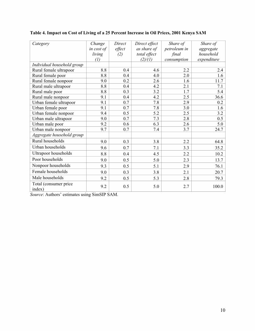
The overall increase in the cost of living to households is estimated at 9.2 percent (table 4 and figure 1). The aggregate increase in the cost of living is lower than the increases for most of the household categories because of the large share of rural male nonpoor households in aggregate households expenditure (36.6 percent) together with the lower cost of living increase for this group (9.1 percent).

10

Table 4. Impact on Cost of Living of a 25 Percent Increase in Oil Prices, 2001 Kenya SAM Category Change

in cost of living

(1)

Direct effect

(2)

Direct effect as share of total effect

(2)/(1)

Share of petroleum in

final consumption

Share of aggregate household

expenditure Individual household group Rural female ultrapoor 8.8 0.4 4.6 2.2 2.4 Rural female poor 8.8 0.4 4.0 2.0 1.6 Rural female nonpoor 9.0 0.2 2.6 1.6 11.7 Rural male ultrapoor 8.8 0.4 4.2 2.1 7.1 Rural male poor 8.8 0.3 3.2 1.7 5.4 Rural male nonpoor 9.1 0.4 4.2 2.5 36.6 Urban female ultrapoor 9.1 0.7 7.8 2.9 0.2 Urban female poor 9.1 0.7 7.8 3.0 1.6 Urban female nonpoor 9.4 0.5 5.2 2.5 3.2 Urban male ultrapoor 9.0 0.7 7.3 2.8 0.5 Urban male poor 9.2 0.6 6.3 2.6 5.0 Urban male nonpoor 9.7 0.7 7.4 3.7 24.7 Aggregate household group Rural households 9.0 0.3 3.8 2.2 64.8 Urban households 9.6 0.7 7.1 3.3 35.2 Ultrapoor households 8.8 0.4 4.5 2.2 10.2 Poor households 9.0 0.5 5.0 2.3 13.7 Nonpoor households 9.3 0.5 5.1 2.9 76.1 Female households 9.0 0.3 3.8 2.1 20.7 Male households 9.2 0.5 5.3 2.8 79.3 Total (consumer price index)

9.2 0.5 5.0 2.7 100.0

Source: Authors’ estimates using SimSIP SAM.

11

Figure 1. Change in Cost of Living as a Result of 25 Percent Increase in Oil Price, by Gender and Poverty Status, 2001 Kenya SAM

Source: Authors’ estimates using SimSIP SAM.

The results suggest that the impact of an oil price increase on household expenditure could be large. This result is not surprising given that petroleum imports represented 2.5 percent of GDP and 7.2 percent of total imports in 2001. Households spent only 2.7 percent of their total consumption on oil, but oil is used in many sectors of the economy, which means that the multiplier or indirect effects are large. Indeed, oil represented 15.9 percent of all intermediate consumption,5 and the sector exhibits strong forward linkages, meaning that it affected by other sectors’ growth more strongly than the average sector in the economy is. Oil exhibits strong backward linkages in the price model, which means that it can affect prices in other sectors more than the average sector does (by construction, strong forward linkages in the quantity-based SAM model translate into strong backward linkages in the price-based SAM model).

Two findings stand out. First, for both rural and urban households, the richer a household is, the greater the impact an increase in oil prices is likely to have (figure 2). Second, urban

5. The comparable figures were 5.6 percent in Lesotho in 2000, 1.1 percent in Tanzania in 2001, 4.1 percent in South Africa in 2000, and 11.1 percent in Uganda in 1999, according to SAMs for these countries.

8.2

8.4

8.6

8.8

9.0

9.2

9.4

9.6

9.8

10.0

Perc

enta

ge c

hang

e

Rural female Rural male Urban female Urban maleUltra poor Ultra Ultra Ultra Poor Poor Poor PoorNon poor Non poor Non poor Non poor

12

households tend to be affected by increases in oil prices more than rural households. The greater impact on richer households can be explained mainly by their larger consumption shares for oil; electricity, gas, and water; and education. The larger consumption share devoted to oil-related products makes the impact of the shock greater for these households, despite the fact that very poor households tend to devote a higher proportion of their total income to consumption. Put differently, these sectors are among the most severely affected by oil price increases, and richer households tend to consume larger shares than poorer households of the goods and services these sectors produce.

Two conclusions can be drawn from analysis of the price changes in various sectors resulting from a 25 percent increase in the price of oil. First, an increase in the price of oil affects nonpoor households more than it affects ultrapoor households (a 25 percent increase in the price of oil generates a 9.3 percent increase in the cost of living among the nonpoor and an 8.8 percent among the ultrapoor) (figure 2). Second, the increase in the price of oil affects male-headed households slightly more than it affects female-headed households (a 25 percent increase in the price of oil generates a 9.2 percent increase in the cost living for households headed by males and a 9.0 percent increase for households headed by females) (figure 3). The consumption shares for oil and utilities (electricity, gas, and water) following the oil price shock (the relative prices of which rise) determine the types of households in which the shock increases the cost of living more (both ultrapoor and male-headed households consume higher shares of oil and utilities).

Figure 2. Price Changes and Contribution to Change in Cost of Living for Nonpoor and Ultrapoor Households as a Result of 25 Percent Increase in Oil Price, 2001 Kenya SAM

Source: Authors’ estimates using SimSIP SAM. Note: A point above the dotted horizontal line (which represents equal contributions for both types of households) indicates that an increase in the price of oil has a greater impact on the cost of living of nonpoor households than ultrapoor households.

0

5

10

15

20

25

30

Oil

Ele

ctric

ity, g

as, a

nd w

ater

Edu

catio

n

Non

met

allic

prod

ucts

Fis

hin

g

Hea

lth

Ow

ned

hou

sing

Veg

etab

les

Oth

er li

vest

ock

Pul

ses

Tea

Milk

and

dai

ry

Roo

ts a

nd tub

ers

Bee

f and

Vea

l

Coffe

e (g

reen

)

Suga

r ca

ne

Fru

its

For

est

ry a

nd

logg

ing

Text

iles

Food

Tra

nspo

rt

Wood

and

pap

er

Oth

er p

riva

te s

ervi

ces

Oth

er c

erea

ls

Mai

ze

Met

al p

rodu

cts

Oth

er ch

emic

als

Tot

al

Perc

enta

ge p

rice

chan

ge

-0.6

-0.4

-0.2

0.0

0.2

0.4

0.6

Impa

ct o

n co

st o

f liv

ing

of n

onpo

or h

ouse

hold

–

impa

ct o

n co

st o

f liv

ing

of u

ltrap

oor h

ouse

hold

Price change Non poor - Ultra poor

13

Figure 3. Price Change and Contribution to Change in Cost of Living for Male- and Female-Headed Households as a Result of 25 Percent Increase in Oil Prices, 2001 Kenya SAM

Source: Authors’ estimates using SimSIP SAM.

Note: A point above the dotted horizontal line (which represents equal contributions for both types of households) indicates that an increase in the price of oil has a greater impact on the cost of living of households headed by men than on the cost of living of households headed by women.

Decomposition of the multiplier effects indicates that 65–75 percent of the final effect of an increase in the price oil on households is explained by closed-loop (feedback) effects and 20–27 percent by open-loop (inter-accounts) effects (table 5).6 Transfer effects are zero (households belong to the institutions group of accounts and oil belongs to the activities group), so the portion of the price change that is not explained by open- and closed-loop effects is explained by the initial shock.

6. See annex 2 for the decomposition formulas with flexible- and fixed-priced sectors (following Parra and Wodon 2010).

0

5

10

15

20

25

30

Oil

Ele

ctric

ity,

gas,

and

wat

er

Edu

catio

n

Non

met

allic

pro

duct

s

Fis

hing

Hea

lth

Ow

ned

hous

ing

Veg

etab

les

Oth

er li

vest

ock

Pul

ses

Tea

Milk

and

dai

ry

Roo

ts a

nd t

uber

s

Bee

f an

d V

eal

Cof

fee

(gre

en)

Sug

ar c

ane

Fru

its

For

estr

y an

d lo

ggin

g

Tex

tiles

Foo

d

Tra

nspo

rt

Woo

d an

d pa

per

Oth

er p

rivat

e se

rvic

es

Oth

er c

erea

ls

Mai

ze

Met

al p

rodu

cts

Oth

er c

hem

ical

s

Tot

al

Perc

enta

ge p

rice

chan

ge

-0.2

-0.1

-0.1

0.0

0.1

0.1

0.2

0.2

0.3

0.3

Impa

ct o

n co

st o

f liv

ing

of m

ale-

head

ed h

ouse

hold

–

impa

ct o

n co

st o

f liv

ing

of fe

mal

e-he

aded

hou

seho

ld

Price change Male-Female

14

Table 5. Price Multiplier Decomposition (millions of K Sh, except where otherwise indicated) Household group

Multiplier

Open-loop Closed-loop

Closed-loop/ multiplier (percent)

Rural female ultrapoor 35.3 7.6 26.1 73.9Rural female poor 35.2 7.7 26.1 74.2Rural female nonpoor 35.8 8.2 26.7 74.6Rural male ultrapoor 35.2 7.7 26.1 73.9Rural male poor 35.3 8.0 26.2 74.2Rural male nonpoor 36.3 8.7 26.1 71.9Urban female ultrapoor 36.3 7.2 26.3 72.4Urban female poor 36.5 7.4 26.2 71.7Urban female nonpoor 37.5 9.2 26.4 70.4Urban male ultrapoor 35.8 7.4 25.8 72.1Urban male poor 36.6 7.7 26.6 72.7Urban male nonpoor 39.0 10.5 25.6 65.8Source: Authors’ estimates using SimSIP SAM. Note: Figures show response to shock of K Sh 100 million.

Conclusion

This paper uses a SAM–multiplier approach to examine the impact of oil price shocks on various categories of households in Kenya. It identifies which sectors of the economy would be most affected and analyzes the distributional implications of these shocks on households given the patterns of consumption observed for different categories of households.

Two findings stand out. First, the potential impact of an oil price shock is high in Kenya. For a 25 percent increase in oil price, the overall increase in the cost of living to households estimated with the SAM is 9.2 percent. This does not necessarily mean that observed inflation would increase as dramatically. Indeed, households and other economic agents tend to adjust to price changes by modifying their behavior, which tends to reduce the impacts predicted using standard SAM multipliers. Nevertheless, the results suggest that the impact of higher oil prices on household living standards and thereby on poverty could be large. Second, there are differences in impacts according to household groups. As a result of differences in consumption patterns, in both rural and urban areas richer households are likely to be more severely affected by oil price hikes than poorer households, and male-headed households are likely to be more severely affected than female-headed households.

15

Annex 1: SAM Model for Impact of Price Shocks

Algebraically, a SAM is a schematic representation of the flow transactions between different sectors or institutions in an economy. The convention that is used defines the cell ijT of the SAM

as the value of payments from sector/institution j to sector/institution i (see table 1).

Some accounts in the SAM model have to be considered exogenous (that is, expenditures can be set independently of income). The choice usually depends on the nature of the simulation experiment, but government, capital account, and the rest of the world are often candidates.

Let n be the number of endogenous accounts and r n− the number of exogenous accounts. Summing down the jth column of the SAM yields

n r

j ij mji=1 m=n+1

Y T + W= (3)

where jY denotes total expenditures of sector j, and mjW denotes total payments to the mth

exogenous account made by sector j. Let jP denote the price of the good produced by sector j;

jQ the total output (in physical units) of sector j; and ijs the amount of sector i’s good (in

physical units) used by sector j. Equation (3) can then be rewritten as

n r

j j i ij m mji=1 m=n+1

P Q Ps + P s= . (4)

Dividing both sides by jQ yields

n r

i ij m mjj

i=1 m=n+1j j

Ps P sP = +

Q Q . (5)

Denote the physical technical coefficients for the endogenous accounts as ijij

j

sc =

Q for

1,...i n= , and define r

m mjj

m=n+1 j

P sb =

Q as the value of total payments to exogenous accounts per

physical unit of sector j’s output. Equation (5) can then be rewritten as

n

j i ij ji=1

P = Pc +b (6)

which implies that the price of output of sector j is a weighted average of the prices of goods sector j buys, with weights given by the physical technical coefficients plus exogenous payments per unit of sector j’s output. Using matrix notation, the resulting system of price equations can be written as

16

=C +′P P B (7)

where C′ is the transpose of ijC= c . The system defined in equation (7) can be solved (under

mild conditions [see ten Raa 2005, theorem 2.1]) as

( ) 1= I C

−′−P B (8)

which is known as the Leontief price formation model.

At first sight, this price model does not seem to be very useful, because the physical technical coefficients are very rarely available. Instead, value technical coefficients ija can be

computed by dividing each cell in T by the respective column sum. The matrix ijA= a is

usually referred to as the technical coefficients matrix, where ijij r

kjk=1

Ta =

T. According to Blair and

Miller (1985), these value-based technical coefficients can also be given a physical interpretation using “dollars worth of output” as a measure of physical quantity. Under this interpretation, because the physical measure is equivalent to the monetary measure, all prices are equal to one. In physical terms the technical coefficient ija represents the dollar’s worth of output of sector i

per each dollar worth of output of sector j. Equations (7) and (8) then become

= A +′P P B (9)

and

( ) 1= I A =M

−′ ′−P B B . (10)

One of the key features of the SAM model is the constancy of the technical coefficients implied by the excess capacity assumption for all sector/institutions. This implies not only the constancy of the physical technical coefficients but also the constancy of the price ratio (for details see Miller and Blair 1985 or Moses 1974):

( ) 1Δ = I A Δ

−′−P B (11)

which means that the effect on prices of a change in the exogenous payments per unit of output (or simply a change in exogenous per unit costs) is given by the inverse (multiplier) matrix

( ) 1M = I A

−′ ′− . Because all prices are equal to one, the absolute change in prices/costs is exactly

equal to the percentage change.

The economic interpretation of most of the prices in the model is straightforward. The prices of activities can be understood as producer prices, the prices of commodities as consumer prices, and the prices of production factors as rental payments for their use. The price of households can be understood as a cost of living index, because it is computed as a weighted

17

average of all the goods the households buy (in and outside the household) plus tax payments. In this paper we consider government, capital account, and the rest of the world accounts to be exogenous. Because the shock studied is an increase in the price of oil, which is usually either controlled by the government or a function of international oil prices, we also set the oil commodity account as exogenous, which means that we actually model the commodity oil as a supply-constrained commodity.

18

Annex 2: Block Decomposition of the Multiplier Matrix

Cell jim of the multiplier matrix M′ in equation (10) quantifies the effect of a unitary change in

sector i’s cost in the price of sector j.7 To decompose the matrix M′ , for any n x n matrix, the nonsingular matrix A equation (9) can be rewritten as

( )= A A +A +′ −P P P B (12)

( ) 1*=A + I A−

−P P B (13)

where

( ) ( )1*A = I A A A

−′− − .8 (14)

Multiplying through by *A yields

( )2 1* * *A =A +A I A−

−P P B . (15)

From equation (13), we have an expression for *A P ; replacing it on the left-hand side yields

( )( )2 1* *=A + I+A I A−

−P P B . (16)

Multiplying equation (16) through by 2*A and replacing the expression for

2*A P from (15) yields

( ) ( )( )3 21 1* * *= I A I+A +A I A− −

− −P B . (17)

Notice that we just decomposed multiplicatively the multiplier matrix M′ from (10) into three different matrices. Define

( ) 1

1M = I A−

− , ( )2* *2M = I+A +A , and ( )3 1

*3M = I A

−− . (18)

Then 3 2 1M=M M M . It is also possible to present the decomposition in an additive way, as

follows:

7. This section is adapted from Parra and Wodon (2008a), who provide expressions for the block decomposition of the multiplier matrix under price constraints. 8. For details on computation, see Pyatt and Round (1979).

19

( ) ( ) ( )1 2 1 3 2 1M=I+ M I + M I M + M I M M

TR OL CL

− − − (19)

where the first term (the identity matrix) is the initial unitary injection. The matrix M1 captures the net effect of a group of accounts on itself through direct transfers, the matrix M2 captures all net effects between partitions, and the matrix M3 captures the net effect of circular income multipliers among endogenous accounts. The terms in the additive decomposition labeled TR (for transfer effects), OL for (open-loop effects), and CL (for closed-loop effects) have broadly the same interpretation as the corresponding multiplicative effects (the matrices Mi).

The n x n matrix A (partition of A′ ) was chosen as follows:

11

33

A 0 0

A= 0 0 0

0 0 A

′ ′

where the first row and column correspond to the activities/commodities group, the second to the production factors, and the third to enterprises/households:

Using the definition of *A from (14),

( ) ( )( )

( )

1

11 211

*32

11333

I A 0 0 0 A 0

A = I A A A = 0 I 0 0 0 A

A 0 00 0 I A

−

−

−

′ ′− ′ ′− − ′ ′ −

( )

( )

1* *12 12 11 21

* *23 23 32

* 1*31 31 33 13

0 A 0 A = I A A

= 0 0 A , A =A

A 0 0 A = I A A

−

−

′ ′ − ′ ′ ′−

. (20)

Using the expression for *A and the definitions in (18) yields

( )

( )

1

11

1

1

33

I A 0 0

M = 0 I 0

0 0 I A

−

−

′− ′−

(21)

* * *12 12 23

* * *2 23 31 23

* * *31 31 12

I A A A

M = A A I A

A A A I

(22)

20

( )( )

( )

1* * *12 23 31

1* * *3 23 31 12

1* * *31 12 23

I A A A 0 0

M = 0 I A A A 0

0 0 I A A A

−

−

−

− −

−

. (23)

We now provide expressions for the matrices TR, OL, and CL defined in equation (19):

( )

( )

1

11

1

33

I A I 0 0

TR= 0 0 0

0 0 I A I

−

−

′− − ′− −

(24)

( )

( ) ( )

( )

1* * *12 12 23 33

1 1* * *23 31 11 23 33

1* * *31 11 31 12

0 A A A I A I

OL= A A I A I 0 A I A I

A I A I A A 0

−

− −

−

′− − ′ ′− − − −

′ − −

(25)

( ) ( )( ) ( )

( ) ( )

1 1* * * * * *3,11 11 3,11 12 3,11 12 23 33

1 1* * * * * *3,22 23 31 11 3,22 3,22 23 33

1 1* * * * * *3,33 31 11 3,33 31 12 3,33 33

M I A M A M A A I A

CL= M A A I A M M A I A

M A I A M A A M I A

− −

− −

− −

′ ′− − ′ ′− −

′ ′− −

(26)

where

( )( )( )

1* * * *3,11 12 23 31

1* * * *3,22 23 31 12

1* * * *3,33 31 12 23

M = I A A A I

M = I A A A I

M = I A A A I

−

−

−

− − − − − −

.

We now interpret and describe some features of the matrices TR, OL, and CL defined in equation (19). TR, which quantifies the net effect (with respect to the initial unitary shock) of groups of accounts into themselves (intra), is a block diagonal matrix with an identity matrix in the second block on the diagonal, a consequence of the absence of transfers among production factors. OL, which captures the net direct effect (with respect to the matrix 1M ) between (inter)

accounts, has zeros along the diagonal. The matrix that captures the net closed-loop effects (with respect to the product 2 1M M ), CL, has no special structure.

Because the price of oil is assumed to be given by the international market, oil is modeled as a fixed-price sector (the equivalent of a supply-constrained sector in the value model). This

21

means that the price of the sector can be increased from its current level only exogenously. Following the notation used by Lewis and Thorbecke (1992) after adapting it to the price model, we show that the final effects on prices, given an exogenous price shock, are given by

( )

( )

1

ncnc nc ncm

c c c c

I C 0 I Qd = d =M d

R I 0 I C

− ′− ′ ′ ′ ′− − − −

p b b

b p p (27)

where ncp is a vector of prices of unconstrained sectors; cb is a vector of endogenous costs for

fixed-price sectors; ncC is a matrix of expenditure propensities among unconstrained sectors

(using average expenditure propensities [technical coefficients]; R is a matrix of expenditure propensities of unconstrained sectors on fixed-price sectors; Q is a matrix of expenditure

propensities of fixed-price sectors on unconstrained sectors; cC is a matrix of expenditure

propensities among fixed-price sectors; ncb is a vector of exogenous costs for unconstrained

sectors; cp is a vector of exogenous prices of fixed-price sectors; I is the conformable identity

matrix; 0 is the null matrix; mM is the mixed multiplier matrix; and the prime symbol (')

denotes the transpose of a matrix.

Using the formula for the inverse of partitioned matrices, we can rewrite the effect of the shock on the unconstrained sectors as

( )

( )( )

( ) ( )

1 1

nc ncnc nc ncm

c nc nc nc c c

I C I C Qd = d =M d

R I C R I C Q + I C

− − ′ ′ ′− − ′ ′ ′ ′ ′ ′ ′− − − − −

p b b

b p p. (28)

In the case in which only a single sector is shocked, the shock vector becomes c

dp

0, where

cdp is the size of the shock. From equation (28), we know that

( ) 1

nc ncd =0.25 I C−′ ′−p Q (29)

where ( ) 1

ncI C−′− is an inverse matrix computed using the matrix of expenditure propensities

after deleting the column and row corresponding to the fixed-price sector (oil in this case) and Q is a vector of oil expenditure propensities for unconstrained sectors. Under mild conditions (see ten Raa 2005, theorem 2.1), the inverse of equation (29) exists and can be decomposed as explained in equation (19). In this case the open-loop effect of the ith term of ncdp is the dot

product of the ith row of the open-loop matrix derived from the inverse matrix ( ) 1

ncI C−′− and

the vector of expenditure propensities Q . The same is true for the transfer and closed-loop effects.

22

References Adelman, I., and J. Edward Taylor. 1990. “A Structural Adjustment with a Human Face Possible? The

Case of Mexico.” Journal of Development Studies 26 (3): 387–407.

Arndt, C., H. Jensen, and F. Tarp. 2000. “Structural Characteristics of the Economy of Mozambique: A SAM–Based Analysis.” Review of Development Economics 4 (3): 292–306.

Bautista, R., S. Robinson, and Moataz El-Said. 2001. “Alternative Industrial Development Paths for Indonesia: SAM and CGE Analyses.” In Restructuring Asian Economics for the New Millennium, vol. 9B, ed. J. Behrman, M. Dutta, S.L. Husted, P. Sumalee, C. Suthiphand and P. Wiboonchutikula, 773–90. Amsterdam: Elsevier Science/North Holland.

Defourny, J., and E. Thorbecke. 1984. “Structural Path Analysis and Multiplier Decomposition within a Social Accounting Matrix Framework.” Economic Journal 94 (373): 111–36.

Dorosh, Paul A. 1994. “Adjustment, External Shocks, and Poverty in Lesotho: A Multiplier Analysis.” Working Paper 71, Cornell Food and Nutrition Program, Ithaca, NY.

Dick, H., S. Gupta, D. Vincent, and H. Voigt. 1984. “The Effect of Oil Price Increases on Four Oil-Poor Developing Countries: A Comparative Analysis.” Energy Economics 6 (1): 59–70.

Jorgenson, Dale. 1984. “Econometric Methods for Applied General Equilibrium Analysis.” In Applied General Equilibrium Analysis, ed. H. E. Scarf and J. B. Shoven, 139–203. New York: Cambridge University Press.

———, ed. 1998. Growth Volume 2: Energy, the Environment, and Economic Growth. Cambridge, MA: MIT Press.

Karingi, S. N., and M. Siriwardana. 2003. “A CGE Model Analysis of Effects of Adjustment to Terms of Trade Shocks on Agriculture and Income Distribution in Kenya.” Journal of Developing Areas 37 (1): 87–108.

Khan, H. A. 1999. “Sectoral Growth and Poverty: A Multiplier Decomposition Analysis for South Africa.” World Development 27 (3): 521–30.

Kumar, P. 2005. Oil Price Increase and the Kenyan Economy. World Bank, AFTP2, Washington, DC.

Leontief, Wassily. 1951. The Structure of the American Economy 1919–1939, 2nd ed. New York: Oxford University Press.

———. 1953. Studies in the Structure of the American Economy. New York: Oxford University Press.

Lewis, B., and E. Thorbecke. 1992. “District-Level Economic Linkages in Kenya: Evidence Based on a Small Regional Social Accounting Matrix.” World Development 20 (6): 881–97.

Miller, R., and P. Blair. 1985. Input-Output Analysis: Foundations and Extensions. Upper Saddle River, NJ: Prentice Hall.

Mitra, P. K. 1994. Adjustment in Oil-Importing Developing Countries: A Comparative Economic Analysis. Cambridge: Cambridge University Press.

Moses, L. 1974. “Output and Prices in Interindustry Models.” Papers of the Regional Science Association 32 (1): 7–18.

Nganou, Jean-Pascal Nguessa. 2005. A Multisectoral Analysis of Growth Prospects for Lesotho: SAM-Multiplier Decomposition and Computable General Equilibrium Perspectives. Ph.D. thesis, Department of Economics, American University, Washington, DC.

Parikh, A., and E. Thorbecke. 1996. “Impact of Rural Industrialization on Village Life and Economy: A Social Accounting Matrix Approach.” Economic Development and Cultural Change 44 (2): 351–77.

23

Parra, J. C., and Q. Wodon. 2008a. “Decomposition of SAM Multipliers under Supply Constraints: Derivation and Application to Oil Price Shocks in Senegal.” World Bank, Development Dialogue on Values and Ethics, Washington, DC.

———. 2010. “SimSIP SAM: Policy Analysis under a SAM Framework.” World Bank, Development Dialogue on Values and Ethics, Washington, DC.

Pyatt, G., and J. Round. 1979. “Accounting and Fixed Price Multipliers in a Social Accounting Matrix Framework.” Economic Journal 89 (356): 850–73.

Roland-Holst, D., and F. Sancho. 1995. “Modeling Prices in a SAM Structure.” Review of Economics and Statistics 77 (2): 361–71.

Round, Jeffery I. 1985. “Decomposing Multipliers for Economic Systems Involving Regional and World Trade.” Economic Journal 95 (378): 383–99.

———. 1989. “Decomposition of Input-Output and Economy-Wide Multipliers in a Regional Setting.” In Frontiers of Input-Output Analysis, ed. Ronald E. Miller, Karen R. Polenske, and Adam Z. Rose, 103–118. Oxford: Oxford University Press.

Semboja, H. 1994. “The Effects of Energy Taxes on the Kenyan Economy: A CGE Analysis.” Energy Economics16 (3): 205–15.

Stone, J. R. N. 1985. “The Disaggregation of the Household Sector in the National Accounts.” In Social Accounting Matrices: A Basis for Planning, ed. G. Pyatt and J. I. Round, 145–85. Washington, DC: World Bank.

Taylor, J. Edward, and I. Adelman. 1996. Village Economies. New York: Cambridge University Press.

Taylor, J. Edward, Antonio Yunez-Naude, George A. Dyer, Micki Stewart, and Sergio Ardila. 2002. “The Economics of ‘Eco-Tourism’: A Galapagos Island Economywide Perspective.” Economic Development and Cultural Change 51 (4): 977–97.

Ten Raa, Thijs. 2005. The Economics of Input-Output Analysis. Cambridge: Cambridge University Press. Thorbecke, Erik. 2000. “The Use of Social Accounting Matrices in Modeling.” Paper prepared for the 26th General Conference of the International Association for Research in Income and Wealth, Cracow, Poland, August 27–September 2.

Thorbecke, Erik, and Hong-Sang Jung. 1996. “A Multiplier Decomposition Method to Analyze Poverty Alleviation.” Journal of Development Economics 48 (2): 279–300.

U.S. Department of Energy. 2004. Country Analysis Brief: Great Lakes Region. Energy Information Administration, Washington, DC.

Wobst, P., and B. Schraven. 2004. “The 2001 Social Accounting Matrix (SAM) for Kenya.” International Food Policy Research Institute, Washington, DC.