Embed Size (px)
Citation preview

MPRAMunich Personal RePEc Archive
Decomposing the Marginal ExcessBurden of Australia’s Goods andServices Tax
George Verikios and Jodie Patron and Reza Gharibnavaz
KPMG Economics, Department of Accounting, Finance andEconomics, Griffith University
1 March 2017
Online at https://mpra.ub.uni-muenchen.de/77850/MPRA Paper No. 77850, posted 23 March 2017 14:52 UTC
DECOMPOSING THE MARGINAL EXCESS
BURDEN OF AUSTRALIA’S GOODS AND
SERVICES TAX
George Verikios
KPMG Economics
and
Department of Accounting, Finance and Economics, Griffith University
Jodie Patron, Reza Gharibnavaz
KPMG Economics
Abstract
We estimate the marginal excess burden of the GST and its components. Our results show that the GST is highly distortionary in its treatment of intermediate inputs and investment, but is efficient as applied to household consumption. We also estimate the general equilibrium effects of changes to the GST base and rate, and its removal from investment. The general equilibrium estimates support the marginal excess burden estimates. Our results suggest that the efficiency of the GST could be improved by broadening the consumption base or removing it from investment. Simply increasing the GST rate would be welfare decreasing.
JEL codes: C68, D58, D61, H21, H22.
Keywords: computable general equilibrium, differential incidence, goods and services tax, marginal excess burden, tax reform, value-added tax.
Acknowledgements
The views expressed here are the authors’ and do not necessarily reflect those of their affiliates. We thank Michael Kouparitsas for suggesting the research topic.
2
1. Introduction
The Goods and Services Tax (GST) is a broad-based expenditure tax introduced in
Australia in July 2000 and modelled on the value-added tax (VAT) system popular in many
European countries. It deviated from most European VATs by having a flat and relatively low
rate of 10%. The GST was introduced as part of larger tax package that included: personal
income tax cuts; lump sum compensation for the inflationary effects of the GST for retirees;
abolition of the wholesale sales tax; changes to excise taxes on beer, petrol and tobacco; and the
repeal of a number of State taxes given that GST revenue would form part of Commonwealth
grants to the States (Warren et al., 2005).
The announcement and introduction of the GST led to intense debate about its efficacy and
the move towards greater reliance on indirect taxation and reduced reliance on direct taxation
(McAllister and Bean, 2000). Fifteen years after its introduction, debate over the GST again
intensified in response to the announcement in early 2015 by the Commonwealth government of
a tax review that included the GST (Australian Government, 2015; Bennet, 2015). In contrast,
previous tax reviews had specifically ruled out any changes to the GST, e.g., the Henry Tax
Review (Commonwealth of Australia, 2009). The government’s announcement of a tax review
led to three significant studies evaluating changes to the GST, either in isolation or as part of
broader package of reforms: see Daley and Wood (2015), KPMG (2016a) and Parliamentary
Budget Office (2015).
Australia has one of the lowest GST rates and one of the highest dependencies on income
taxes in the OECD; further, a significant proportion of goods and services in Australia are GST-
free or zero-rated (e.g., basic food, health, education and housing). This suggests that there is the
capacity to broaden the GST base and raise the GST rate, and use the additional revenue to
reduce other taxes, e.g., personal income tax. This view was reflected in the public discussion
following the announcement of the tax review in 2015, and in Daley and Wood (2015), KPMG
(2016a), and Parliamentary Budget Office (2015). All three of these studies analysed increases in
the GST rate and broadening of the GST base, as well as other tax changes. In this paper we
focus on the efficiency of changes to the GST rate, the GST base as well as its application to non-
consumption bases. Although there exist recent estimates of the overall marginal excess burden
(MEB) of the GST (Cao et al., 2015; Independent Economics, 2014), no MEB estimates exist of
3
the non-consumption bases of the GST. As such, our purpose is to inform the debate around the
GST and its components.
To analyse the efficiency of the GST, we apply a dynamic general equilibrium framework
with a high degree of sectoral detail, intersectoral linkages, and a comprehensive representation
of the Australian tax system. The model we apply has been specifically designed for tax policy
analysis. A general equilibrium framework is the preferred approach to analysing major tax
changes. Partial equilibrium analysis of major tax changes can only capture first-round effects
whereas a general equilibrium framework also captures second-round effects and also
interactions across different taxes (Cao et al., 2015). Goulder and Williams (2003) show that
ignoring general equilibrium effects can underestimate the MEB of commodity taxes by a factor
of 10.
Although the GST is often described as a broad-based consumption tax, (e.g., Freebairn,
2013), it is more than this. Australian data show the GST also applies to intermediate inputs,
exports and investment (capital expenditure) (ABS, 2013). Thus, the GST is more accurately
described as a broad-based expenditure tax. We disentangle the efficiency of the GST by
estimating the overall MEB of the GST and the MEB for each expenditure component. Our
results show that the GST has an MEB of 19 cents in its current form and 16 cents with a broader
base that includes basic food, health and education. These results are consistent with recent
estimates in Cao et al. (2015). We estimate the MEB for intermediate inputs and investment to
be 27 and 26 cents; these very high MEBs are offset by much lower MEBs of 22 and 17 cents for
exports and consumption.
We check our MEB estimates against general equilibrium estimates of four scenarios that
modify different aspects of the GST. The scenarios involve a mixture of GST rate increases, base
broadening, and the exemption of capital expenditure. In each case, we ensure the changes are
revenue neutral by holding constant the government budget as a share of GDP via an endogenous
personal income tax rate. The general equilibrium estimates support the MEB estimates by
showing that broadening the consumption base and removing the GST from investment would
increase economic activity and economic welfare. In contrast, raising the GST rate would reduce
economic activity and welfare. Our results suggest that common discussion suggesting that
raising the GST rate would be a low cost source of higher revenue is misplaced and to be
avoided.
4
2. Tax reform and tax revenue in Australia
Tax reform has been at the forefront of Australian government policy over the last two
decades. In 1998 the Commonwealth government released its comprehensive A New Tax System
(ANTS) plan that was the first step towards the introduction of the GST, the removal of
wholesale sales tax, personal tax cuts and the abolition of a raft of other taxes, along with changes
to Australia’s welfare payments system and pensions in 2000 (Warren et al., 2005). The
announcement and introduction of the GST led to intense debate about its efficacy and the move
towards greater reliance on indirect taxation and reduced reliance on direct taxation (McAllister
and Bean, 2000). Around the same time, the Commonwealth government instigated a Review of
Business Taxation (Ralph, 1999). This inquiry resulted in a number of recommendations around
business taxation reform, including the reduction in the headline company tax rate and changes to
depreciation, capital gains, and fringe benefits taxation.
In May 2010, the Australian Treasury released the Henry Tax Review: a comprehensive
study into Australia’s tax and transfer system (Commonwealth of Australia, 2009). This review
provided numerous recommendations for further tax reform, including the recommendation that
efforts to raise government revenue should be focused on four efficient tax bases - personal
income, business income, private consumption expenditure and economic rents from natural
resources and land. Despite the inclusion of consumption expenditure in this list, the GST was
specifically excluded from assessment under the Henry Tax Review and the subsequent 2011
government-hosted Tax Forum.
More recently, the Commonwealth government announced a tax review in early 2015
(Australian Government, 2015; Bennet, 2015). This review differed from previous tax reviews as
it included the GST: previous tax reviews had specifically ruled out any changes to the GST.
Political events overtook the review with no review recommendations released. The
Commonwealth government did propose a cut from 30% to 25% in company income tax in the
2016-17 budget (Australian Government, 2016).
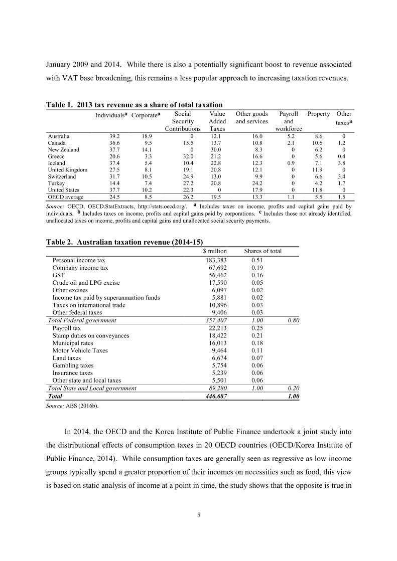
A recent OECD study shows that tax revenues in many OECD countries are now above
their pre-global financial crisis levels (OECD 2014b). Personal and company income taxes are
still the main contributors to government revenues across most of these countries: see Table 1.
OECD (2014a) also finds that there is a general trend towards consumption taxes amongst
member countries. Many countries, particularly European countries, have recently increased
their standard VAT with an increase of 1.5% in the average standard VAT observed between
5
January 2009 and 2014. While there is also a potentially significant boost to revenue associated
with VAT base broadening, this remains a less popular approach to increasing taxation revenues.
Table 1. 2013 tax revenue as a share of total taxation Individualsa Corporatea Social
Security Contributions
Value Added Taxes
Other goods and services
Payroll and
workforce
Property Other
taxesa
Australia 39.2 18.9 0 12.1 16.0 5.2 8.6 0 Canada 36.6 9.5 15.5 13.7 10.8 2.1 10.6 1.2 New Zealand 37.7 14.1 0 30.0 8.3 0 6.2 0 Greece 20.6 3.3 32.0 21.2 16.6 0 5.6 0.4 Iceland 37.4 5.4 10.4 22.8 12.3 0.9 7.1 3.8 United Kingdom 27.5 8.1 19.1 20.8 12.1 0 11.9 0 Switzerland 31.7 10.5 24.9 13.0 9.9 0 6.6 3.4 Turkey 14.4 7.4 27.2 20.8 24.2 0 4.2 1.7 United States 37.7 10.2 22.3 0 17.9 0 11.8 0
OECD average 24.5 8.5 26.2 19.5 13.3 1.1 5.5 1.5
Source: OECD, OECD.StatExtracts, http://stats.oecd.org/. a Includes taxes on income, profits and capital gains paid by
individuals. b Includes taxes on income, profits and capital gains paid by corporations. c Includes those not already identified,
unallocated taxes on income, profits and capital gains and unallocated social security payments.
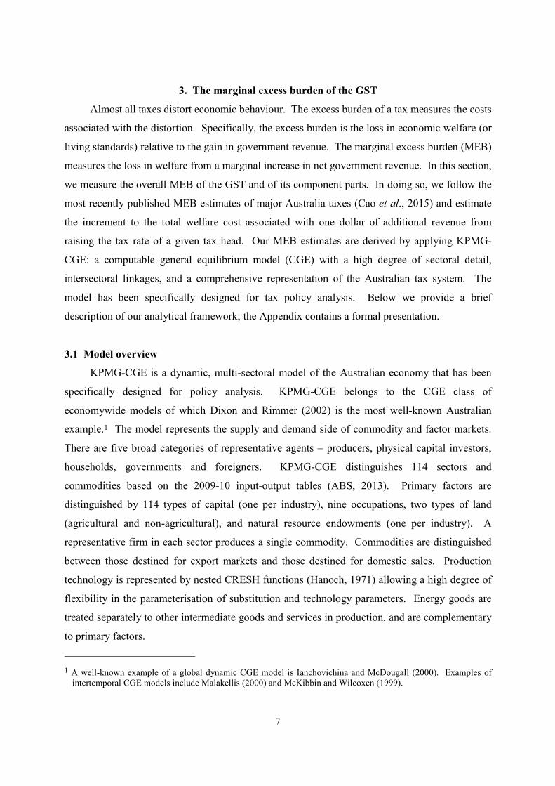
Table 2. Australian taxation revenue (2014-15)
$ million Shares of total
Personal income tax 183,383 0.51 Company income tax 67,692 0.19 GST 56,462 0.16 Crude oil and LPG excise 17,590 0.05 Other excises 6,097 0.02 Income tax paid by superannuation funds 5,881 0.02 Taxes on international trade 10,896 0.03 Other federal taxes 9,406 0.03
Total Federal government 357,407 1.00 0.80
Payroll tax 22,213 0.25 Stamp duties on conveyances 18,422 0.21 Municipal rates 16,013 0.18 Motor Vehicle Taxes 9,464 0.11 Land taxes 6,674 0.07 Gambling taxes 5,754 0.06 Insurance taxes 5,239 0.06 Other state and local taxes 5,501 0.06
Total State and Local government 89,280 1.00 0.20
Total 446,687 1.00
Source: ABS (2016b).
In 2014, the OECD and the Korea Institute of Public Finance undertook a joint study into
the distributional effects of consumption taxes in 20 OECD countries (OECD/Korea Institute of
Public Finance, 2014). While consumption taxes are generally seen as regressive as low income
groups typically spend a greater proportion of their incomes on necessities such as food, this view
is based on static analysis of income at a point in time, the study shows that the opposite is true in

6
most cases when measured as a percentage of expenditure from a lifetime perspective. The study
also suggests that reduced VAT rates with the aim of benefiting lower income groups and
promoting social welfare may not always work as expected in practice. In some cases, higher
income groups benefit more from reduced rates on items such as hotel accommodation and
restaurant food.
Like many other OECD countries, personal income tax (PIT), company income tax (CIT)
and the GST are the three major sources of tax revenue for the Commonwealth government;
Table 2 shows that these three taxes raise 86% of Commonwealth government tax revenue and
69% of revenue for all Australian governments. The table also reflects the huge vertical fiscal
imbalance that is a feature of the distribution of tax powers across levels of government in
Australia. But, it should be noted that all GST revenue is distributed to state governments via the
Commonwealth Grants Commission in the form of untied grants.
Australia’s GST rate of 10% is low compared to the unweighted average GST rate of
19.2% amongst all OECD countries (Table 3). Many observers see this fact as a reason to
consider raising more revenue from the GST than is currently (Daley and Wood, 2015).
Consistent with this, OECD data on tax revenue composition shows that Australia’s total taxation
mix is skewed towards direct taxes, i.e., PIT and CIT (Table 1). According to the OECD, these
taxes contributed almost 60% of total Australian tax revenue in 2013 compared to an OECD
average of just over 30%.
Table 3. GST rates in OECD member countries in 2014 Australia 10.0 Japan 8.0 Austria 20.0 Korea 10.0 Belgium 21.0 Luxembourg 15.0 Canada 5.0 Mexico 16.0 Chile 19.0 Netherlands 21.0 Czech Republic 21.0 New Zealand 15.0 Denmark 25.0 Norway 25.0 Estonia 20.0 Poland 23.0 Finland 24.0 Portugal 23.0 France 20.0 Slovak Republic 20.0 Germany 19.0 Slovenia 22.0 Greece 23.0 Spain 21.0 Hungary 27.0 Sweden 25.0 Iceland 25.5 Switzerland 8.0 Ireland 23.0 Turkey 18.0 Israel 18.0 United Kingdom 20.0 Italy 22.0 USA (Combined State & Local Sales Tax) 1.69 to 9.45
Unweighted average (excluding US) 19.2
Source: Tax Foundation, www.VATlive.com.
7
3. The marginal excess burden of the GST
Almost all taxes distort economic behaviour. The excess burden of a tax measures the costs
associated with the distortion. Specifically, the excess burden is the loss in economic welfare (or
living standards) relative to the gain in government revenue. The marginal excess burden (MEB)
measures the loss in welfare from a marginal increase in net government revenue. In this section,
we measure the overall MEB of the GST and of its component parts. In doing so, we follow the
most recently published MEB estimates of major Australia taxes (Cao et al., 2015) and estimate
the increment to the total welfare cost associated with one dollar of additional revenue from
raising the tax rate of a given tax head. Our MEB estimates are derived by applying KPMG-
CGE: a computable general equilibrium model (CGE) with a high degree of sectoral detail,
intersectoral linkages, and a comprehensive representation of the Australian tax system. The
model has been specifically designed for tax policy analysis. Below we provide a brief
description of our analytical framework; the Appendix contains a formal presentation.
3.1 Model overview
KPMG-CGE is a dynamic, multi-sectoral model of the Australian economy that has been
specifically designed for policy analysis. KPMG-CGE belongs to the CGE class of
economywide models of which Dixon and Rimmer (2002) is the most well-known Australian
example.1 The model represents the supply and demand side of commodity and factor markets.
There are five broad categories of representative agents – producers, physical capital investors,
households, governments and foreigners. KPMG-CGE distinguishes 114 sectors and
commodities based on the 2009-10 input-output tables (ABS, 2013). Primary factors are
distinguished by 114 types of capital (one per industry), nine occupations, two types of land
(agricultural and non-agricultural), and natural resource endowments (one per industry). A
representative firm in each sector produces a single commodity. Commodities are distinguished
between those destined for export markets and those destined for domestic sales. Production
technology is represented by nested CRESH functions (Hanoch, 1971) allowing a high degree of
flexibility in the parameterisation of substitution and technology parameters. Energy goods are
treated separately to other intermediate goods and services in production, and are complementary
to primary factors.
1 A well-known example of a global dynamic CGE model is Ianchovichina and McDougall (2000). Examples of intertemporal CGE models include Malakellis (2000) and McKibbin and Wilcoxen (1999).

8
There is a infinitely-lived representative household agent that owns the major share of
factors of production with foreigners owning the remainder; the representative household can
either spend or save its income. There is a single government sector representing all levels of
government in Australia. The model includes detailed government fiscal accounts including the
accumulation of public assets and liabilities based on ABS (2015). On the revenue side, detailed
modelling of over 20 direct and indirect taxes and income from government enterprises is
included. On the expenditure side, government consumption, investment and payments of
various types of transfers are modelled.
Foreigners supply imports at fixed c.i.f. prices and demand commodities (exports) at
variable f.o.b. prices. The nominal exchange rate is the numeraire. Nevertheless, the real
exchange rate (i.e., the ratio of domestic prices to foreign prices in a common currency) is
endogenous as export prices are an endogenous function of export volumes. Investment
behaviour is industry specific and is positively related to the expected rate of return on capital.
This rate takes into account company taxation, a variety of capital allowances and the structure of
the imputation system. Foreign asset and liability accumulation is explicitly modelled, as are the
cross-border income flows they generate and that contribute to the evolution of the current
account.
The contains three of dynamic mechanisms: capital accumulation; liability accumulation;
and lagged adjustment processes. Capital accumulation is specified separately for each industry.
An industry’s capital stock in year t+1 is its capital in year t plus its investment during year t
minus depreciation. Liability accumulation is specified for the public sector and foreign
accounts. Public sector liability in year t+1 is public sector liability in year t plus the public
sector deficit incurred during year t. Net foreign liabilities in year t+1 are net foreign liabilities in
year t plus the current account deficit in year t plus the effects of revaluations of assets and
liabilities caused by changes in prices. Lagged adjustment processes are specified for the
response of wage rates to gaps between the demand for and the supply of labour by occupation.
A simulation of the effects of a tax policy change involves running the model twice to
create the baseline (or business-as-usual) scenario and the policy scenario. The baseline is
designed to be a plausible forecast of how the economy will evolve in the shortrun in the absence
of the policy shock of interest. Thus, the paths of most macroeconomic variables are exogenous
in the shortrun and set in accordance with forecasts made by a macroeconomic model (KPMG,
2016b). In the longrun, the economy converges to a balanced growth path where all prices and
9
quantities grow by 2.5%. In the policy scenario, all macroeconomic variables are endogenous.
With the exception of the policy variables of interest (e.g., tax rates), all exogenous variables in
the policy scenario are assigned the values they have in the baseline scenario. The differences in
the values of variables in the policy and baseline scenarios quantifies the effects of moving the
variables of interest away from their baseline values.
Total household consumption is assumed to be a function of household disposable income
and the average propensity to consume. In the baseline scenario, the average propensity to
consume is endogenous in the shortrun to allow the model to accommodate exogenous forecasts
for real household consumption; in the longrun consumption converges to balanced growth and
trade is almost balanced. In the policy scenario, real household consumption is endogenous and
the ratio of the trade balance to GDP returns to baseline level in the longrun; this mimics time-
consistent behaviour by households.2 This imposes a budget constraint on household behaviour
in the long run.
Total real investment is the sum of industry demands for investment. Exogenous forecasts
for total investment are imposed in the shortrun in the baseline scenario; in the longrun industry
investment converges to balanced growth. In the policy closure, industry after-tax rates of return
respond to changes in the demand for capital relative to supply in the shortrun but eventually
move to baseline values in the longrun. This ties after-tax rates of return to the global rate of
return. Total real government consumption moves with exogenous forecasts in the baseline
closure; in the policy closure total real government consumption is held at baseline levels.
Expectations by households and investors are assumed to be myopic. It would be
computationally challenging to specify forward-looking expectations for agents in a model of this
size. In recognition of the limitations of this approach, we impose longrun constraints on agents’
behaviour that mimic an equilibrium that would be observed if forward-looking behaviour was
imposed. These constraints are: household consumption adjusts so that the ratio of the trade
balance to GDP returns to baseline level in the longrun, and this ratio is one of balanced trade in
2 Ensuring the ratio of the trade balance to GDP returns to baseline is equivalent to constraining the growth of net foreign liabilities relative to the baseline. Malakellis (2000), Appendix A3.2, shows how constraining the growth of net foreign liabilities is equivalent to enforcing an intertemporal budget constraint on households.
10
the terminal year of the baseline; and industry after-tax rates of return to baseline values in the
longrun.3
3.2 Estimating marginal excess burden
We follow the CGE tax analysis literature and define the MEB as the negative of the
increment to the total welfare cost of the tax system. The increment to the welfare cost is
measured by the equivalent variation (EV), i.e., the amount the household would be willing to
pay to avoid the tax change. Following Cao et al. (2015), the MEB can be expressed in
consumption units as
( ) ( )( )
( )0 0
0 0
0 0
1
1
n
c c
WMEB C C L L
P
τ
τ
−= − + −
+; (1)
where 0C and 0L represent consumption and leisure in the initial (pre-shock) equilibrium, and C
and L represent consumption and leisure after the tax change (i.e., in the post-shock
equilibrium). Thus, ( )0C C− and ( )0L L− are minus the change in consumption and leisure;
this means the MEB is a positive number. The change in leisure is valued at
( ) ( )0 0 0 01 1n c cW Pτ τ− − ; where 0W is the initial wage rate and 0nτ is the initial labour income tax
rate. 0cP is the initial price of household consumption and 0cτ is the tax rate on household
consumption. Hence, leisure is valued at the initial after-tax real wage rate. We hold
( )0 01c cP τ+ constant in equation (1), i.e., ( )0 01c cP τ+ = 1, so that the MEB is valued in dollars.
0C is calibrated using consumption data from the model valued at ( )0 01c cP τ+ . 0L . To
define a value for 0L we assume a leisure share of total waking hours of 0.64, i.e., leisure is
around twice as large as employment.4 This is broadly in line with the macroeconomics literature
that suggests leisure is four times as large as employment (King and Rebelo, 1999). Using this
3 Malakellis (2000) compares myopic expectations with model-consistent expectations for households and investors in an intertemporal CGE model. The results show that the shortrun response to model shocks is very different under each set of expectations. Nevertheless, the longrun results are almost identical.
4 The approach we follow is to assume that the representative household has 168 (=24x7) hours available per week, of which 56 (=8x7) are sleeping hours. This gives 112 (=168-56) waking hours per week. Then, assume the household works 40 hours per week giving 72 (=112-40) leisure hours available per week. Applying this approach gives a leisure share of total waking hours of 0.64 (=72/112).

11
calibration, we normalise the time endowment at 1, and set 0L = 0.64 and employment (E) at
0.36 (= 1 – 0.64). Thus, with a fixed time endowment ( )0L L− , or L∆ , will equal E−∆ .
Our MEB calculations assume the government maintains its initial budget balance via a
lump-sum transfer ( )LST to households when a marginal tax change is imposed. This is what
Musgrave and Musgrave (1973) call ‘differential incidence’.5 For the purposes of comparison
with Cao et al. (2015), we normalise all MEB results on the lump-sum transfer, i.e., MEB LST .
Given this normalisation and that the MEB = –EV, the MEB tells us the welfare impact from
raising net revenue by one dollar. For example, an MEB of 10 cents indicates that there is a net
loss in welfare of 10 cents if an additional dollar is raised in net tax revenue.
3.3 The marginal excess burden of the GST
Economic theory tells us that a necessary condition for optimality is that relative prices
reflect relative marginal rates of transformation and substitution across commodities. Another
way to express this condition is that the marginal social value and marginal social cost of a
commodity should be equal. The existence of zero-rated and nonzero-rated commodities under
the GST violates this condition. Thus, the GST will skew consumption away from nonzero-rated
commodities towards zero-rated commodities. This raises the excess burden of the GST.
Therefore, the excess burden of the GST would be minimised if there were no exemptions; in this
case, the GST would be a generic tax on consumption.
The main effect of the GST is to reduce the after-tax real wage: ( ) ( )1 1W C CW Pτ τ− + ,
where W is the pre-tax wage, CP is the pre-tax consumer price index (CPI), and
Wτ and Cτ are
the tax rates on wages and consumption. A GST raises the after-tax CPI and lowers the after-tax
real wage. Note that a tax on labour income and the GST have identical effects on the after-tax
real wage. A lower after-tax real wage creates a disincentive to supply labour. We calculate the
MEB of the GST, its components and the labour income component of the personal income tax
system: Table 4 presents the results.
We estimate the overall MEB of the GST at 19 cents, i.e., every dollar of GST revenue
causes welfare to fall by 19 cents. This estimate is consistent with Cao et al. (2015).
5 “Differential incidence...measures the difference in the distributional effects of financing a given expenditure by one or another tax” (Musgrave and Musgrave, 1973, p. 358).
12
Nevertheless, these estimates are higher than those calculated in earlier work by KPMG (2010) at
8 cents, KPMG (2011b) at 12 cents and Independent Economics (2014) at 13 cents. We note the
trend of rising MEB estimates for the GST over time. To extent that estimates differ across these
studies, this is likely to differences in (i) the modelling framework applied, (ii) the welfare
measure applied, and in (iii) the assumed uncompensated labour supply elasticity.
Table 4. Marginal excess burden of the GST and personal income tax
GST: Current base
GST: Broader base
Personal income
tax
Total Intermediate inputs
Investment Household consumption
Exports Total
Marginal excess burden ($) 0.19 0.27 0.26 0.17 0.22 0.16 0.18
Revenue ($m)a 54,253 3,785 8,833 40,461 1,175 - 170,313
a GST revenue is calculated from the 2013-14 input-output tables (ABS, 2016a). Personal income tax revenue is for
2013-14 and is taken from ABS (2016b)
We also estimate the MEB of a broader-based GST that applies to consumption of basic
food, health and education. This lowers the overall MEB to 16 cents. Cao et al. (2015) estimate
the MEB of a broader-based GST at 17 cents. We go beyond previous studies and estimate the
MEB of each expenditure base upon which the GST applies. For household consumption, the
MEB is low at 16 cents. For exports, the MEB is higher at 22 cents. For intermediate inputs and
investment, the MEB rises sharply to 27 and 26 cents. The overall MEB of the GST is the
revenue-weighted average of the individual components. The results illuminate an oft ignored
aspect of the GST: it is an expenditure tax rather than a consumption tax.6 This distinction is
important as 25% of GST revenue is raised from non-consumption bases. For exports, GST
revenue is raised on expenditure by tourists mainly on accommodation, food and beverage
services and transport.7 These taxes apply despite the GST being ‘destination-based’ and thus
exempting exports (Freebairn, 2013). However, only 2% of GST revenue is raised from exports.
The next largest expenditure base is intermediate inputs at 7%. Given this is a tax on
production, the base is rather elastic and this gives a relatively high MEB of 27 cents. Here the
GST applies to goods and services used by firms in three sectors: finance, insurance and
superannuation funds, and dwellings, with each contributing about one-third of GST on
6 We thank Michael Kouparitsas for making us aware this point. 7 Other expenditure categories include telecommunications, internet services, rental and hiring services, sport,
performing arts, and gambling.
13
intermediate inputs. This base represents the input-tax nature of the GST as it applies to financial
services and construction of dwellings. As Freebairn (2013) notes, “The complicated GST
provisions relating to financial services mean that households are under-taxed via the non-
taxation of value-added financial services, whereas businesses are over-taxed through being
unable to claim GST offsets on financial services they purchase.” (p. 39).
The largest non-consumption GST base is investment at 16% with an MEB similar to
intermediate inputs at 26 cents. This base mainly applies to dwellings, machinery and equipment,
and other capital expenditure used as inputs to investment. Taxing inputs to investment will
lower the after-tax rate of return on capital: ( ) ( )1 1K I IR Pτ τ− + , where R is the pre-tax rental
rate, IP is the pre-tax price of investment, and
Kτ and Iτ are the tax rates on capital and
investment. For a capital importer such as Australia, the after-tax rate of return on capital is set
on global capital markets. A fall in the after-tax return on capital reduces capital inflows (and
capital usage) until the after-tax rate of return increases to again equal the global rate. Thus,
investment and capital are very elastic tax bases.8 Further, there are indirect effects from the fall
in capital usage caused by an investment tax. Lower capital usage will reduce the marginal
product of labour and discourage the use of labour by firms until the real wage rate falls to match
the marginal product of labour. Lucas (1990) shows that the effects on the labour market of
capital taxes can be significant, a result supported by many studies cited therein.
The decomposed MEB results suggest that economic welfare could be improved by
reallocating the GST base away from investment expenditure and towards consumption
expenditure; this would be substituting a low MEB base (consumption) for a high MEB base
(investment). We focus on investment as this aspect of the GST raises 16% of total GST
revenue. This, combined with a high MEB, suggests there could be major economic benefits
from substituting consumption expenditure for investment expenditure in the GST base. We
explore these benefits in the next section.
4. General equilibrium estimates of GST changes
Taking the MEB estimates from Section 3 as a guide, we estimate the general equilibrium
effects of four tax reform scenarios.
Scenario 1: a 10% GST on a broader base, i.e., including basic food, health and education.
8 See Cao et al (2015), pp. 14-17 for further discussion of these effects.

14
Scenario 2: a 12.25% GST on the current base.
Scenario 3: a 15.2% GST on non-investment expenditure, i.e., removal of the GST from
investment expenditure and an increase in the rate to 15.2% on non-investment expenditure on
the current base.
Scenario 4: an 11.9% GST on non-investment expenditure and a broader base, i.e., removal of
the GST from investment expenditure, an increase in the rate to 11.9% on other expenditure and a
broadening of the base to include basic food, health and education.
We impose all scenarios in 2018-19. Scenario 1 is estimated to raise an additional $14.1
billion in GST revenue. The tax rates in scenarios 2-4 have been calibrated to raise the identical
amount of extra GST revenue as Scenario 1. In this way, the scenarios are equivalent in terms of
the first-order effects on government revenue. The additional GST revenue is returned to
households through personal income tax (PIT) cuts in order to maintain the government budget
balance as a share of GDP at its initial level; this ensures the scenarios are equivalent in terms of
the first-order effects on household income. Table 4 shows that the MEB for PIT is
approximately equal to that for the overall GST (18 cents). As the extra GST revenue is returned
to households as lower personal income taxes, the scenarios are also equivalent in terms of their
MEB and their first-order effect on post-tax wage rates. This equivalence across scenarios means
that the real output and welfare effects across scenarios will largely reflect the marginal excess
burden of each tax change. This provides a guide on which tax scenarios are to be preferred on
an efficiency basis; the results should be consistent with the MEB results in Table 4.
4.1 Shortrun results
Figure 1 presents the effects on real GDP for each scenario: all scenarios show a
contraction in economic activity in 2018-19. In the initial year, capital stocks cannot respond due
to gestation lags. Thus, GDP can only change from a change in employment. The initial effect
on employment is similar in all scenarios. So, for simplicity, we explain this mechanism using
Scenario 1. The effect on employment is driven by the effect of the GST on the consumption
price index (CPI); the CPI rises due to the broadening of the GST base (Figure 2). As wage rates
in the current period are determined by (i) wage rates in the previous period indexed by current
inflation, and (ii) labour market conditions, wage rates are sticky in the shortrun and flexible in
the longrun. As wages rates rise due to the increase in the CPI and the output price received by
firms falls, the cost of labour for firms rises and they reduce their labour usage.

15
-1.0
-0.8
-0.6
-0.4
-0.2
0.0
0.2
0.4
2017
2018
2019
2020
2021
2022
2023
2024
2025
2026
2027
2028
2029
2030
2031
2032
2033
2034
2035
2036
2037
2038
2039
2040
2041
2042
2043
2044
2045
2046
2047
scenario 1 scenario 2 scenario 3 scenario 4
Figure 1. GDP effects – all scenarios (percentage change)
-1.5
-1.3
-1.1
-0.9
-0.7
-0.5
-0.3
-0.1
0.1
0.3
0.5
0.7
2017
2018
2019
2020
2021
2022
2023
2024
2025
2026
2027
2028
2029
2030
2031
2032
2033
2034
2035
2036
2037
2038
2039
2040
2041
2042
2043
2044
2045
2046
2047
CPI wage rate output price employment
Figure 2. Prices and employment – scenario 1 (percentage change)
-0.3
-0.2
-0.1
0.0
0.1
0.2
0.3
20172018
2019
20202021202220232024202520262027
20282029
2030
20312032203320342035203620372038
2039
20402041204220432044204520462047
scenario 1 scenario 2 scenario 3 scenario 4
Figure 3. Capital stock – all scenarios (percentage change)
-2.5
-2.0
-1.5
-1.0
-0.5
0.0
0.5
1.0
1.5
20172018201920202021202220232024202520262027202820292030
20312032203320342035203620372038203920402041204220432044204520462047
scenario 1 scenario 2 scenario 3 scenario 4
Figure 4. Investment – all scenarios (percentage change)
16
-2.5
-2.2-1.9
-1.6
-1.3
-1.0-0.7
-0.4
-0.1
0.20.5
0.8
1.1
2017
2018
2019
2020
2021
2022
2023
2024
2025
2026
2027
2028
2029
2030
2031
2032
2033
2034
2035
2036
2037
2038
2039
2040
2041
2042
2043
2044
2045
2046
2047
scenario 1 scenario 2 scenario 3 scenario 4
Figure 5. Price of investment – all scenarios (percentage change)
-1.5
-1.3
-1.0
-0.8
-0.5
-0.3
0.0
0.3
0.5
2017
2018
2019
2020
2021
2022
2023
2024
2025
2026
2027
2028
2029
2030
2031
2032
2033
2034
2035
2036
2037
2038
2039
2040
2041
2042
2043
2044
2045
2046
2047
scenario 1 scenario 2 scenario 3 scenario 4
Figure 6. Employment – all scenarios (percentage change)
-2.2
-1.9
-1.6
-1.3
-1.0
-0.7
-0.4
-0.1
0.2
0.5
2017
2018
2019
2020
2021
2022
2023
2024
2025
2026
2027
2028
2029
2030
2031
2032
2033
2034
2035
2036
2037
2038
2039
2040
2041
2042
2043
2044
2045
2046
2047
scenario 1 scenario 2 scenario 3 scenario 4
Figure 7. Consumption – all scenarios (percentage change)
-1.5
-1.3
-1.1
-0.9
-0.7
-0.5
-0.3
-0.1
0.1
0.3
0.5
0.7
2017
2018
2019
2020
2021
2022
2023
2024
2025
2026
2027
2028
2029
2030
2031
2032
2033
2034
2035
2036
2037
2038
2039
2040
2041
2042
2043
2044
2045
2046
2047
scenario 1 scenario 2 scenario 3 scenario 4
Figure 8. Imports - all scenarios (percentage change)
17
-1.0
-0.7
-0.4
-0.1
0.2
0.5
2017
2018
2019
2020
2021
2022
2023
2024
2025
2026
2027
2028
2029
2030
2031
2032
2033
2034
2035
2036
2037
2038
2039
2040
2041
2042
2043
2044
2045
2046
2047
scenario 1 scenario 2 scenario 3 scenario 4
Figure 9. Output price – all scenarios (percentage change)
-0.7
-0.5
-0.3
-0.1
0.1
0.3
0.5
0.7
0.9
2017
2018
2019
2020
2021
2022
2023
2024
2025
2026
2027
2028
2029
2030
2031
2032
2033
2034
2035
2036
2037
2038
2039
2040
2041
2042
2043
2044
2045
2046
2047
scenario 1 scenario 2 scenario 3 scenario 4
Figure 10. Exports – all scenarios (percentage change)
From 2019-20, real GDP shows positive deviations from baseline in all scenarios reflecting
the response in capital stocks to the changes in investment in 2018-19 (Figures 3 and 4). With
investment higher in 2018-19 in Scenarios 3 and 4, capital stocks are larger in 2019-20; the
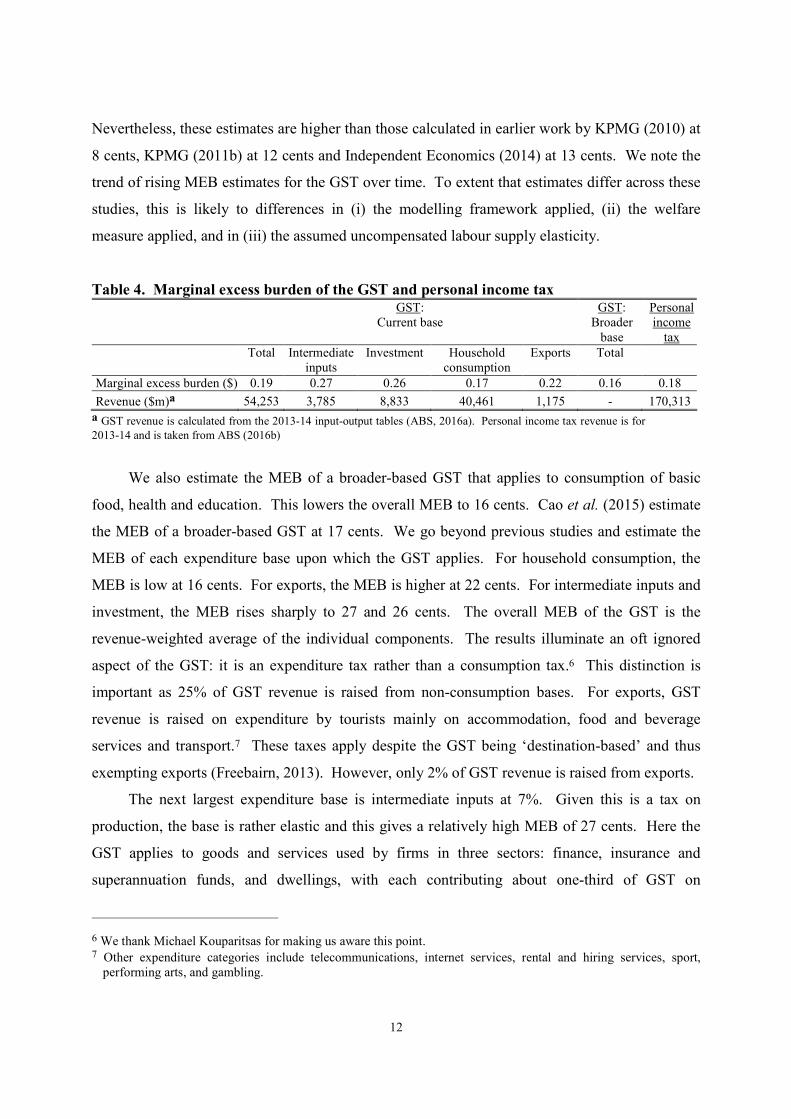
opposite is true for Scenarios 1 and 2. With investment a function of the rate of return (the ratio
of the rental price to the price of investment), the large fall in the price of investment in Scenarios
3 and 4 drives the large positive response in investment in the initial year (Figure 5). The price of
investment falls by much less in Scenarios 1 and 2 in 2018-19, thus the rate of return falls and
this drives investment below baseline. The relative differences in the price of investment across
scenarios reflects the removal of the GST from investment in Scenarios 3 and 4 whereas the GST
on investment is maintained in Scenario 1 and increased in Scenario 2.
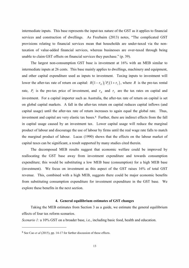
From 2019-20, the excess supply of labour created in 2018-19 is slowly reduced as wage
rates mainly respond to labour market conditions and there are no further shocks to the CPI from
changes in the GST (Figure 6). Thus, employment is above baseline in all scenarios until 2024-
25. This combined with the positive capital deviations causes GDP to be above baseline in all
scenarios over this period. By 2024-25, the labour market has largely returned to baseline
18
conditions in scenarios 1 and 2 with the unemployment rate unchanged from its initial level.
Capital stocks have also largely settled down by 2024-25 in Scenarios 1 and 2.
For Scenarios 3 and 4 the story is different. The strong investment response in the initial
year causes a strong capital stock response in the following years. By 2023-24 this causes rates
of return to overshoot and show negative deviations. This drives investment below baseline in
2024-25, which drives employment below baseline in 2024-25 and 2025-26 before returning to
baseline in 2026-27. The overshooting in rates of return reflects the assumption of myopic
expectations by investors.
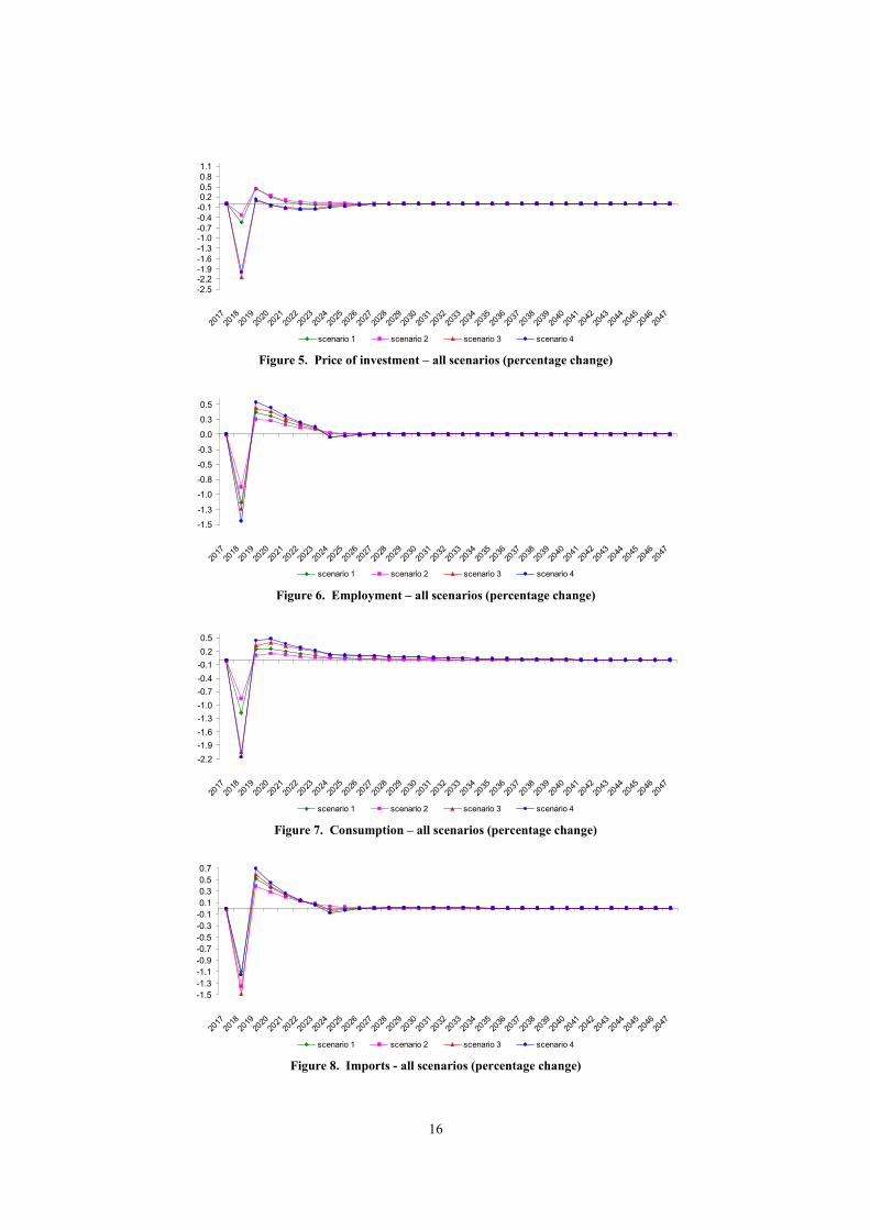
In the shortrun, household consumption moves with household disposable income as the
saving rate is fixed. As already observed, the tax change reduces employment and wage rates in
the initial year; thus, wage income falls. Capital income also falls as the fall in employment
reduces demand for capital and the rental price of capital. Lower disposable household income
means lower consumption at a fixed saving rate (Figure 7). From 2018-19 onwards, household
consumption is above baseline as household income recovers from higher wage and capital
income. Imports closely follow the movements in household consumption (Figure 8).
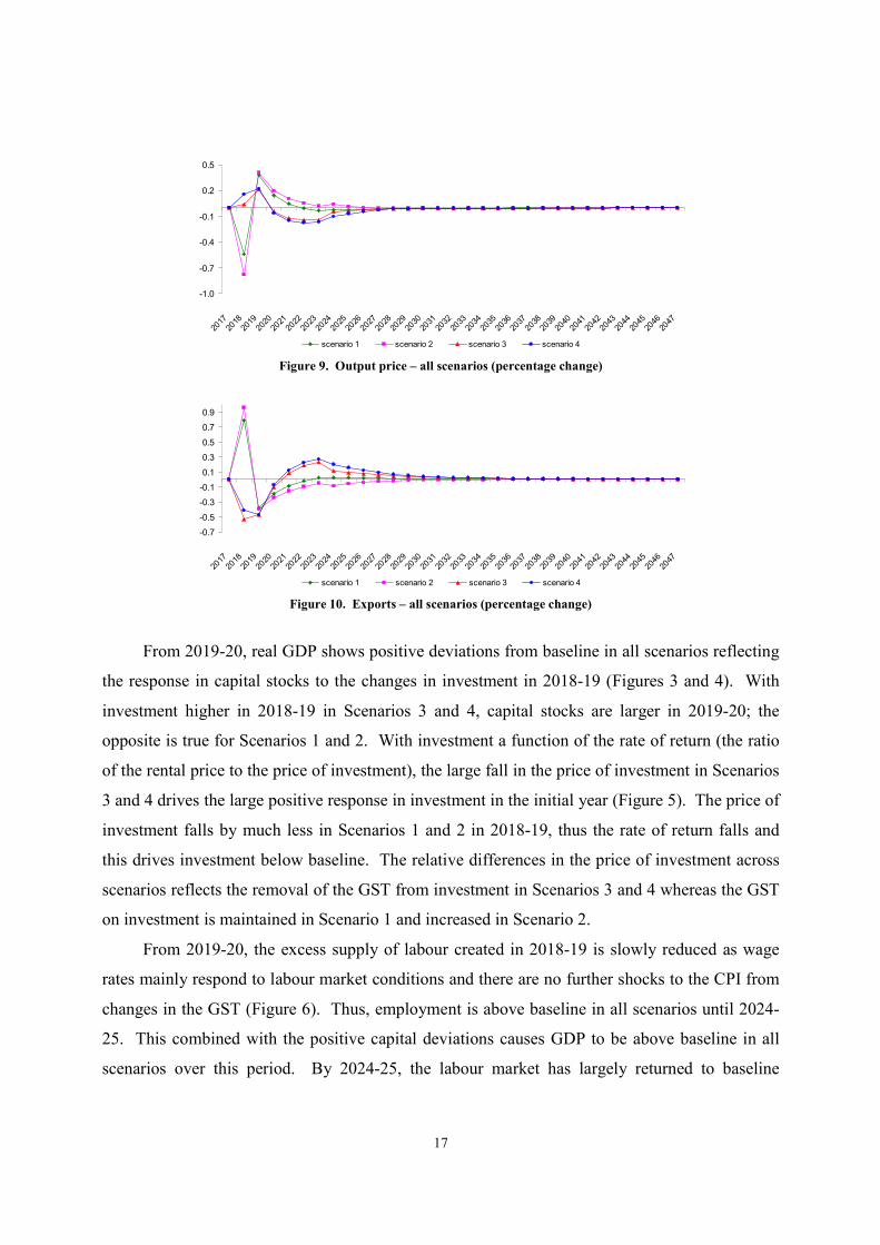
The export response depends on the investment response. In Scenarios 1 and 2, investment
is lower in the initial year. This lowers domestic absorption and production costs (Figure 9).
Lower production costs make exports cheaper to foreigners and sales increase (Figure 10). The
opposite occurs in Scenarios 3 and 4. Investment is higher in the initial year, which leads to
higher production costs, higher export prices and lower export sales. From 2019-20, the export
responses are similar across scenarios; exports are below baseline. This reflects output prices
moving above baseline in all scenarios, which is driven by the beginning of clearing the labour
market of excess supply. As output prices are above baseline, export prices are higher and sales
are lower.
In the longrun, the saving rate is endogenous and adjusts so as to ensure the trade balance to
GDP ratio returns to baseline. Thus, we observe that exports slowly move towards baseline in
Scenarios 1 and 2 as the trade balance to GDP ratio initially improves from the tax change. In
Scenarios 3 and 4, the trade balance to GDP ratio initially worsened from the tax change; thus,
exports must move above baseline.
19
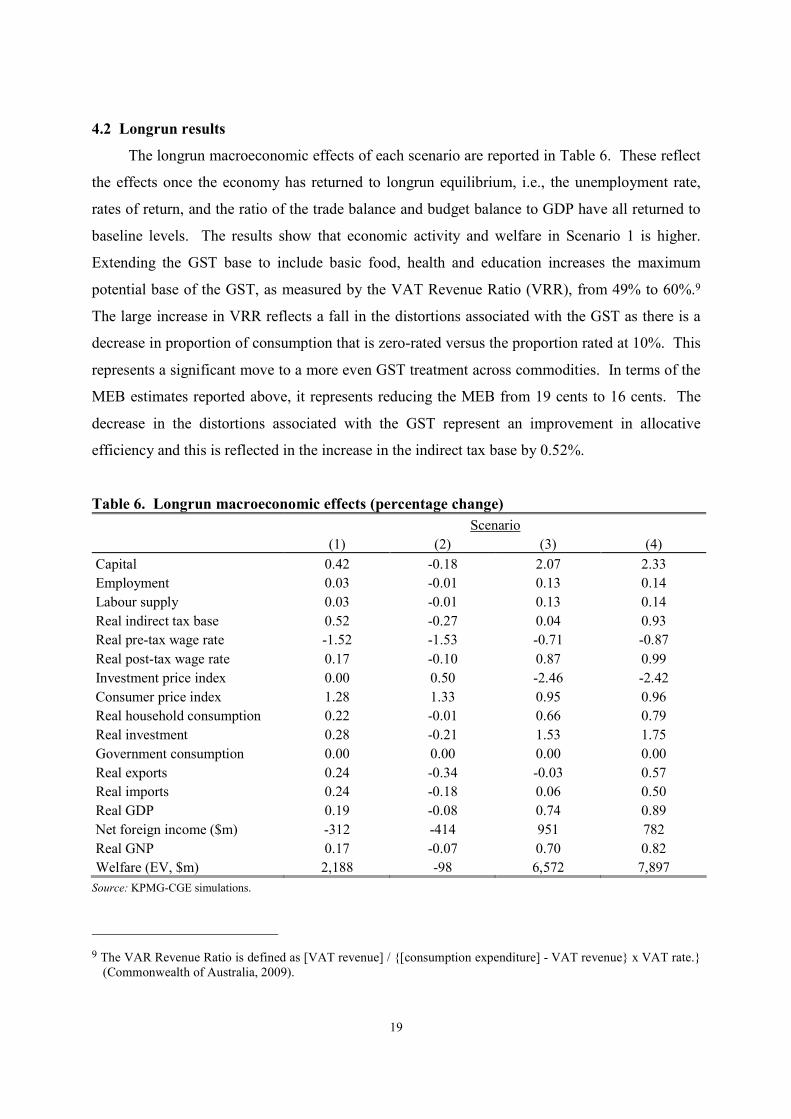
4.2 Longrun results
The longrun macroeconomic effects of each scenario are reported in Table 6. These reflect
the effects once the economy has returned to longrun equilibrium, i.e., the unemployment rate,
rates of return, and the ratio of the trade balance and budget balance to GDP have all returned to
baseline levels. The results show that economic activity and welfare in Scenario 1 is higher.
Extending the GST base to include basic food, health and education increases the maximum
potential base of the GST, as measured by the VAT Revenue Ratio (VRR), from 49% to 60%.9
The large increase in VRR reflects a fall in the distortions associated with the GST as there is a
decrease in proportion of consumption that is zero-rated versus the proportion rated at 10%. This
represents a significant move to a more even GST treatment across commodities. In terms of the
MEB estimates reported above, it represents reducing the MEB from 19 cents to 16 cents. The
decrease in the distortions associated with the GST represent an improvement in allocative
efficiency and this is reflected in the increase in the indirect tax base by 0.52%.
Table 6. Longrun macroeconomic effects (percentage change)
Scenario
(1) (2) (3) (4)
Capital 0.42 -0.18 2.07 2.33
Employment 0.03 -0.01 0.13 0.14
Labour supply 0.03 -0.01 0.13 0.14
Real indirect tax base 0.52 -0.27 0.04 0.93
Real pre-tax wage rate -1.52 -1.53 -0.71 -0.87
Real post-tax wage rate 0.17 -0.10 0.87 0.99
Investment price index 0.00 0.50 -2.46 -2.42
Consumer price index 1.28 1.33 0.95 0.96
Real household consumption 0.22 -0.01 0.66 0.79
Real investment 0.28 -0.21 1.53 1.75
Government consumption 0.00 0.00 0.00 0.00
Real exports 0.24 -0.34 -0.03 0.57
Real imports 0.24 -0.18 0.06 0.50
Real GDP 0.19 -0.08 0.74 0.89
Net foreign income ($m) -312 -414 951 782
Real GNP 0.17 -0.07 0.70 0.82
Welfare (EV, $m) 2,188 -98 6,572 7,897
Source: KPMG-CGE simulations.
9 The VAR Revenue Ratio is defined as [VAT revenue] / {[consumption expenditure] - VAT revenue} x VAT rate.} (Commonwealth of Australia, 2009).
20
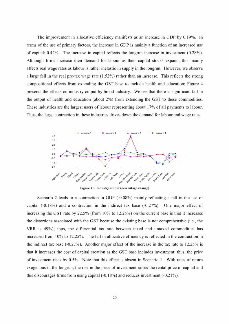
The improvement in allocative efficiency manifests as an increase in GDP by 0.19%. In
terms of the use of primary factors, the increase in GDP is mainly a function of an increased use
of capital: 0.42%. The increase in capital reflects the longrun increase in investment (0.28%).
Although firms increase their demand for labour as their capital stocks expand, this mainly
affects real wage rates as labour is rather inelastic in supply in the longrun. However, we observe
a large fall in the real pre-tax wage rate (1.52%) rather than an increase. This reflects the strong
compositional effects from extending the GST base to include health and education; Figure 4
presents the effects on industry output by broad industry. We see that there is significant fall in
the output of health and education (about 2%) from extending the GST to these commodities.
These industries are the largest users of labour representing about 17% of all payments to labour.
Thus, the large contraction in these industries drives down the demand for labour and wage rates.
-2.5
-1.5
-0.5
0.5
1.5
2.5
3.5
4.5
Agriculture
Mining
Manuf
Utilities
Construction
Whole Trade
Retail Trade
Accom Food
Transport
Info Telec
Fin Ins
Rent Hire Dwell
Prof Sci Tech
Admin Supp
Public Admin
Educ Train
Health Care
Arts Rec
Other Serv
scenario 1 scenario 2 scenario 3 scenario 4
Figure 11. Industry output (percentage change)
Scenario 2 leads to a contraction in GDP (-0.08%) mainly reflecting a fall in the use of
capital (-0.18%) and a contraction in the indirect tax base (-0.27%). One major effect of
increasing the GST rate by 22.5% (from 10% to 12.25%) on the current base is that it increases
the distortions associated with the GST because the existing base is not comprehensive (i.e., the
VRR is 49%); thus, the differential tax rate between taxed and untaxed commodities has
increased from 10% to 12.25%. The fall in allocative efficiency is reflected in the contraction in
the indirect tax base (-0.27%). Another major effect of the increase in the tax rate to 12.25% is
that it increases the cost of capital creation as the GST base includes investment: thus, the price
of investment rises by 0.5%. Note that this effect is absent in Scenario 1. With rates of return
exogenous in the longrun, the rise in the price of investment raises the rental price of capital and
this discourages firms from using capital (-0.18%) and reduces investment (-0.21%).
21
The importance of the distorting effect of the GST on investment is reflected in the strength
of the increase in GDP in Scenario 3, where the GST is removed from investment but increased
to 15.2% on the current base. Real GDP expands by 0.74% driven mainly by a large increase in
the use of capital (2.07%) and a small increase in the use of labour (0.13%). The strong increase
in the use of capital is driven by a fall in the rental price of capital that accompanies the 2.46%
fall in the price of investment. With rates of return exogenous in the longrun, the fall in the price
of investment decreases the rental price of capital, which encourages firms to use more capital
and increase investment by 1.53%.
Scenario 4 combines elements of Scenario 1 and 3 by extending the GST to include basic
food, health and education, and removing the GST from investment. Nevertheless, the GST rate
must only rise to 11.9% (cf. 15.2% in Scenario 3) in order to raise the same amount of GST
revenue as in the other scenarios. Thus, the GDP response in Scenario 4 is close to the sum of
the GDP responses in Scenarios 1 and 3: 0.89% versus 0.93% (= 0.19% + 0.74%). Scenario 4
leads to the largest increase in GDP driven by the effects already described in Scenarios 1 and 3:
a strong increase in the use of capital (2.33%) and the indirect tax base (0.93%). This is
consistent with the results observed for Scenarios 1 and 3.
In all scenarios the employment response small as it is limited by the longrun increase in
the labour supply: as the unemployment rate returns to baseline levels in the longrun, the increase
in employment matches the increase in labour supply. Labour supply is weakly responsive to
real after-tax wage rates. Real after-tax wage rates respond more favourably than pre-tax wage
rates, as the PIT rate falls in all scenarios due to the increase in GST revenue.
The industry effects are presented in Figure 11 aggregated from 114 sectors to the 19
industry divisions used in the national accounts . The results are largely as expected. Extending
the GST base to basic food, health and education reduces the size of these sectors (Scenarios 1
and 4). Removal of investment from the GST base increases demand for construction, which is
the main input to investment and dwellings (Scenarios 3 and 4). Highly capital intensive sectors,
such as mining and finance, also benefit from the removal of the GST from investment.
Accommodation and food services also contract noticeably in scenarios where the GST increases
the most (Scenarios 2 and 3); this is mainly driven by lower export sales. Arts and recreation
services also contract noticeably in Scenarios 2 and 3, mainly driven by lower sales to
households.
22
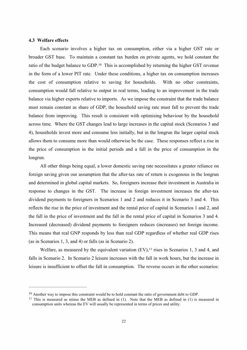
4.3 Welfare effects
Each scenario involves a higher tax on consumption, either via a higher GST rate or
broader GST base. To maintain a constant tax burden on private agents, we hold constant the
ratio of the budget balance to GDP.10 This is accomplished by returning the higher GST revenue
in the form of a lower PIT rate. Under these conditions, a higher tax on consumption increases
the cost of consumption relative to saving for households. With no other constraints,
consumption would fall relative to output in real terms, leading to an improvement in the trade
balance via higher exports relative to imports. As we impose the constraint that the trade balance
must remain constant as share of GDP, the household saving rate must fall to prevent the trade
balance from improving. This result is consistent with optimising behaviour by the household
across time. Where the GST changes lead to large increases in the capital stock (Scenarios 3 and
4), households invest more and consume less initially, but in the longrun the larger capital stock
allows them to consume more than would otherwise be the case. These responses reflect a rise in
the price of consumption in the initial periods and a fall in the price of consumption in the
longrun.
All other things being equal, a lower domestic saving rate necessitates a greater reliance on
foreign saving given our assumption that the after-tax rate of return is exogenous in the longrun
and determined in global capital markets. So, foreigners increase their investment in Australia in
response to changes in the GST. The increase in foreign investment increases the after-tax
dividend payments to foreigners in Scenarios 1 and 2 and reduces it in Scenario 3 and 4. This
reflects the rise in the price of investment and the rental price of capital in Scenarios 1 and 2, and
the fall in the price of investment and the fall in the rental price of capital in Scenarios 3 and 4.
Increased (decreased) dividend payments to foreigners reduces (increases) net foreign income.
This means that real GNP responds by less than real GDP regardless of whether real GDP rises
(as in Scenarios 1, 3, and 4) or falls (as in Scenario 2).
Welfare, as measured by the equivalent variation (EV),11 rises in Scenarios 1, 3 and 4, and
falls in Scenario 2. In Scenario 2 leisure increases with the fall in work hours, but the increase in
leisure is insufficient to offset the fall in consumption. The reverse occurs in the other scenarios:
10 Another way to impose this constraint would be to hold constant the ratio of government debt to GDP. 11 This is measured as minus the MEB as defined in (1). Note that the MEB as defined in (1) is measured in
consumption units whereas the EV will usually be represented in terms of prices and utility.
23
leisure decreases as work hours rise, but the increase in consumption more than offsets the
decrease in leisure.
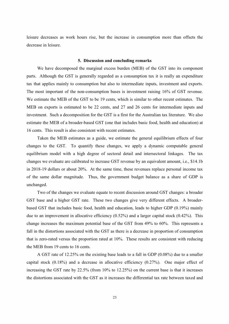
5. Discussion and concluding remarks
We have decomposed the marginal excess burden (MEB) of the GST into its component
parts. Although the GST is generally regarded as a consumption tax it is really an expenditure
tax that applies mainly to consumption but also to intermediate inputs, investment and exports.
The most important of the non-consumption bases is investment raising 16% of GST revenue.
We estimate the MEB of the GST to be 19 cents, which is similar to other recent estimates. The
MEB on exports is estimated to be 22 cents, and 27 and 26 cents for intermediate inputs and
investment. Such a decomposition for the GST is a first for the Australian tax literature. We also
estimate the MEB of a broader-based GST (one that includes basic food, health and education) at
16 cents. This result is also consistent with recent estimates.
Taken the MEB estimates as a guide, we estimate the general equilibrium effects of four
changes to the GST. To quantify these changes, we apply a dynamic computable general
equilibrium model with a high degree of sectoral detail and intersectoral linkages. The tax
changes we evaluate are calibrated to increase GST revenue by an equivalent amount, i.e., $14.1b
in 2018-19 dollars or about 20%. At the same time, these revenues replace personal income tax
of the same dollar magnitude. Thus, the government budget balance as a share of GDP is
unchanged.
Two of the changes we evaluate equate to recent discussion around GST changes: a broader
GST base and a higher GST rate. These two changes give very different effects. A broader-
based GST that includes basic food, health and education, leads to higher GDP (0.19%) mainly
due to an improvement in allocative efficiency (0.52%) and a larger capital stock (0.42%). This
change increases the maximum potential base of the GST from 49% to 60%. This represents a
fall in the distortions associated with the GST as there is a decrease in proportion of consumption
that is zero-rated versus the proportion rated at 10%. These results are consistent with reducing
the MEB from 19 cents to 16 cents.
A GST rate of 12.25% on the existing base leads to a fall in GDP (0.08%) due to a smaller
capital stock (0.18%) and a decrease in allocative efficiency (0.27%). One major effect of
increasing the GST rate by 22.5% (from 10% to 12.25%) on the current base is that it increases
the distortions associated with the GST as it increases the differential tax rate between taxed and
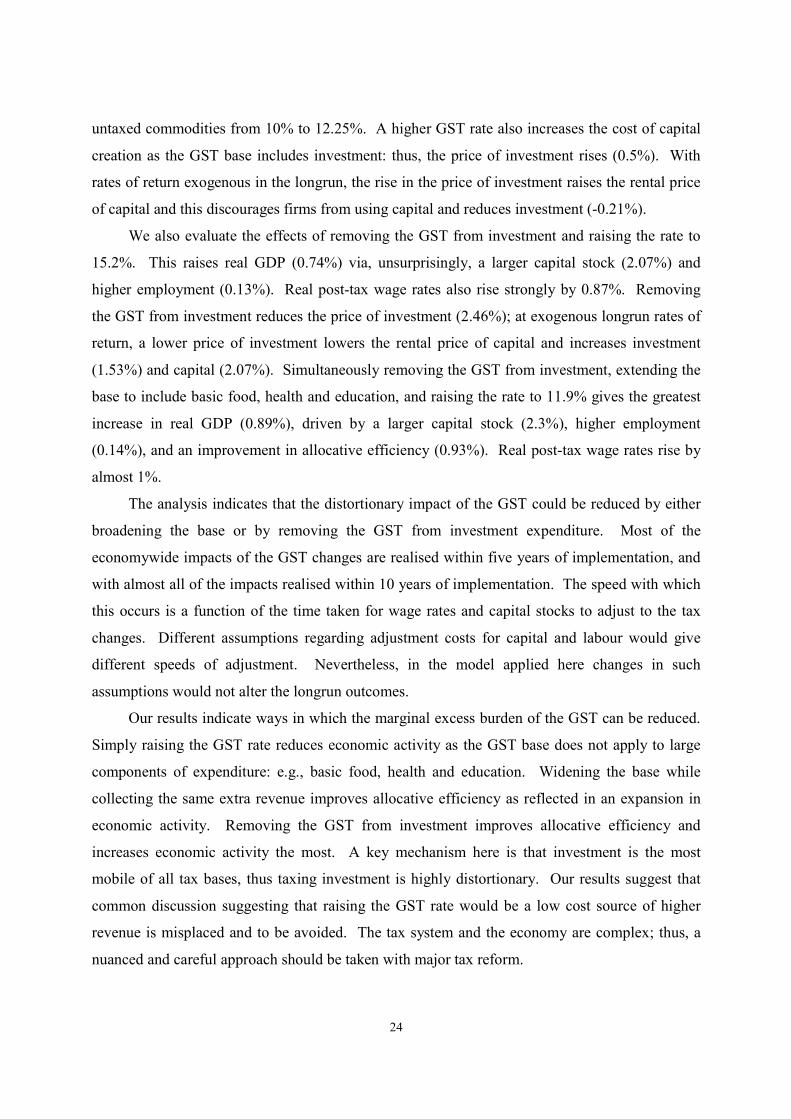
24
untaxed commodities from 10% to 12.25%. A higher GST rate also increases the cost of capital
creation as the GST base includes investment: thus, the price of investment rises (0.5%). With
rates of return exogenous in the longrun, the rise in the price of investment raises the rental price
of capital and this discourages firms from using capital and reduces investment (-0.21%).
We also evaluate the effects of removing the GST from investment and raising the rate to
15.2%. This raises real GDP (0.74%) via, unsurprisingly, a larger capital stock (2.07%) and
higher employment (0.13%). Real post-tax wage rates also rise strongly by 0.87%. Removing
the GST from investment reduces the price of investment (2.46%); at exogenous longrun rates of
return, a lower price of investment lowers the rental price of capital and increases investment
(1.53%) and capital (2.07%). Simultaneously removing the GST from investment, extending the
base to include basic food, health and education, and raising the rate to 11.9% gives the greatest
increase in real GDP (0.89%), driven by a larger capital stock (2.3%), higher employment
(0.14%), and an improvement in allocative efficiency (0.93%). Real post-tax wage rates rise by
almost 1%.
The analysis indicates that the distortionary impact of the GST could be reduced by either
broadening the base or by removing the GST from investment expenditure. Most of the
economywide impacts of the GST changes are realised within five years of implementation, and
with almost all of the impacts realised within 10 years of implementation. The speed with which
this occurs is a function of the time taken for wage rates and capital stocks to adjust to the tax
changes. Different assumptions regarding adjustment costs for capital and labour would give
different speeds of adjustment. Nevertheless, in the model applied here changes in such
assumptions would not alter the longrun outcomes.
Our results indicate ways in which the marginal excess burden of the GST can be reduced.
Simply raising the GST rate reduces economic activity as the GST base does not apply to large
components of expenditure: e.g., basic food, health and education. Widening the base while
collecting the same extra revenue improves allocative efficiency as reflected in an expansion in
economic activity. Removing the GST from investment improves allocative efficiency and
increases economic activity the most. A key mechanism here is that investment is the most
mobile of all tax bases, thus taxing investment is highly distortionary. Our results suggest that
common discussion suggesting that raising the GST rate would be a low cost source of higher
revenue is misplaced and to be avoided. The tax system and the economy are complex; thus, a
nuanced and careful approach should be taken with major tax reform.

25
There are two aspects of GST reform that are beyond the scope of this analysis but are
nevertheless important. It is expected that there would be changes in compliance costs associated
with changes to the GST of the form analysed here. While these costs are likely to be one-off
and relatively small, they should be considered as part of any policy design process. Further,
given the regressivity of the GST, some of the changes to the GST of the type suggested here
would be expected to impart negative real income effects on lower income groups. These effects
need to be countered by an adequate and well-designed compensation package.

26
References
ABS (Australian Bureau of Statistics) (2013), Australian National Accounts: Input-Output Tables, 2009-
10, Cat. no. 5209.0.55.001, ABS, Canberra, September.
—— (2016a), Australian National Accounts: Input-Output Tables, 2013-14, Cat. no. 5209.0.55.001, ABS, Canberra, June.
—— (2015). Government Finance Statistics, Australia, 2013-14, Cat. no. 5512.0, Australian Bureau of Statistics, Canberra, May.
—— (2016b), Taxation Revenue, Australia, 2014-15, Cat. no. 5506.0, ABS, Canberra, April.
Adams, P.D., Horridge, J.M. and Parmenter, B.R. (2000), MMRF-GREEN: A Dynamic, Multi-Sectoral,
Multi-Regional Model of Australia, Centre of Policy Studies/IMPACT Centre, Working Paper OP-94, Monash University, October.
ATO (Australian Taxation Office) (2015), Taxation Statistics, 2012-13, www.ato.gov.au/About-ATO/Research-and-statistics/In-detail/Taxation-statistics/Taxation-statistics-2012-13, April.
Australian Government (2015), Re:think, Tax Discussion Paper, Australian Government, Canberra, March.
Australian Government (2016), Economy-wide modelling for the 2016-17 Budget, Commonwealth of Australia, Canberra, May.
Commonwealth of Australia (2009), Australia's Future Tax System, Report to the Treasurer, Part One,
Overview, Canberra, December.
Bennet, J. (2015), ‘Tax system up for review after Re:Think discussion paper suggests more reliance on GST: Treasurer’, Australian Broadcasting Corporation, March, http://www.abc.net.au/news/2015-03-30/government-paper-questions-gst-rates,-exemptions/6357110.
Cao, L., Hosking, A., Kouparitsas, M., Mullaly, D., Rimmer, X., Shi, Q., Stark, W. and Wende. S. (2015), Understanding the economy-wide efficiency and incidence of major Australian taxes, Treasury Working Paper 2015-01, April.
Daley, J. and Wood, D. (2015), A GST Reform Package, Grattan Institute Report No. 2015-12, December.
Dandie, S. and Mercante, J. (2007), Australian Labour Supply Elasticities: Comparison and Critical
Review, Treasury Working Paper 2007-04, Australian Government, Canberra.
Dixon, P.B., Parmenter, B.R., Sutton, J. and Vincent, D.P. (1982), ORANI: A Multisectoral Model of the
Australian Economy, Contributions to Economic Analysis 256, North-Holland, Amsterdam.
Dixon, P.B. and Rimmer, M.T. (2002), Dynamic General Equilibrium Modelling for Forecasting and
Policy: A Practical Guide and Documentation of MONASH, Contributions to Economic Analysis 256, North-Holland Publishing, Amsterdam.
——, —— and Wittwer, G. (2011), ‘Saving the Southern Murray-Darling Basin: the economic effects of a buyback of irrigation water’, Economic Record, vol. 87, no. 276, pp. 153–68.
Freebairn, J. (2013), ‘A larger GST in a tax-mix change’, Insights: Melbourne Business and Economics, vol. 13, April, pp 39–43.
Goulder, L. and Williams, R. (2003), ‘The substantial bias from ignoring general equilibrium effects in estimating excess burden, and a practical solution’, Journal of Political Economy, vol. 111, no. 4, pp. 898–927.
Hanoch, G. (1971), ‘CRESH production functions’, Econometrica, vol. 39, September, pp. 695–712.
Harrison, W.J. and Pearson, K.R. (1996), ‘Computing solutions for large general equilibrium models using GEMPACK’, Computational Economics, vol. 9, no. 2, pp. 83–127.
Horridge, M., Madden, J. and Wittwer, G. (2005), ‘The impact of the 2002-2003 drought on Australia’, Journal of Policy Modeling, vol. 27, no. 3, pp. 285–308.
27
Independent Economics (2014), Economic Impacts of Negative Gearing of Residential Property, Report prepared for the Housing Industry Association, July.
Johansen, L. (1960), A Multisectoral Study of Economic Growth, North-Holland, Amsterdam.
King, R.G. and Rebelo, S.T. (1999), ‘Resuscitating real business cycles’, Chapter 14, pp. 927–1007 in Taylor, J.B. and Woodford, M. (eds.), Handbook of Macroeconomics, Elsevier Science, Amsterdam.
KPMG (2010), CGE Analysis of the Current Australian Tax System, Canberra.
—— (2011b), Economic Analysis of the Impacts of Using GST to Reform Taxes, Report Prepared for CPA Australia, September, Canberra.
—— (2016a), The Economic Impact of GST-funded Company Tax Cut, January.
—— (2016b), Quarterly Economic Outlook, August.
Lucas, R.E. (1990), ‘Supply-side economics: An analytical review’, Oxford Economic Papers: New
Series, vol. 42, no. 2, pp. 293–316.
McAllister, I and Bean, C. (2000), ‘The electoral politics of economic reform in Australia: The 1998 election’, Australian Journal of Political Science, vol. 35, no. 3, pp. 383–99.
McKibbin, W.J. and Wilcoxen, P.J. (1999), ‘The theoretical and empirical structure of the G-Cubed model’, Economic Modelling, vol. 16, issue 1, pp. 123–48.
Musgrave, R.A. and Musgrave, P.B. (1973), Public Finance in Theory and Practice, McGraw-Hill, New York.
Organisation of Economic Cooperation and Development (OECD) (2014a), Consumption Tax Trends 2014: VAT/GST and excise rates, trends and policy issues, OECD Publishing.
—— (2014b), Revenue Statistics 2014, OECD Publishing.
—— and Korea Institute of Public Finance (2014), The Distributional Effects of Consumption Taxes in OECD Countries, OECD Tax Policy Studies, No. 22, OECD Publishing.
Parliamentary Budget Office (2015), Goods and Services Tax, Distributional Analysis and Indicative
Reform Scenarios, Report no. 05/2015, Parliament of Australia, Canberra, December.
Ralph, J. (1999), Review of Business Taxation: A Tax System Redesigned, Report of the Ralph Committee, Australian Government Publishing Service, Canberra, July.
Romer, D. (2001), Advanced Macroeconomics, 2nd ed., McGraw-Hill, Boston.
Shoven, J.B. and Whalley, J. (1984), ‘Applied general-equilibrium models of taxation and international trade: An introduction and survey’, Journal of Economic Literature, vol. 22, no. 3, pp. 1007–51.
Stone, R. (1954), ‘Linear expenditure systems and demand analysis: an application to the pattern of British demand’, The Economic Journal, vol. LXIV, pp. 511–27.
Theil, H. 1980, The System-Wide Approach to Microeconomics, The University of Chicago Press, Chicago.
Vincent, D.P., Dixon, P.B., & Powell, A.A. (1980), ‘The estimation of supply response in Australian agriculture: The CRESH/CRETH production system’, International Economic Review, vol. 21, no. 1, pp. 221–242.
Warren, N., Harding, A. and Lloyd, R. (2005), ‘GST and the changing incidence of Australian taxes: 1994-95 to 2001-02’, eJournal of Tax Research, vol. 3, no. 1, pp. 114–45.
Wittwer, G., McKirdy, S. and Wilson, R. (2005), ‘Regional economic impacts of a plant disease incursion using a general equilibrium approach’, Australian Journal of Agricultural and Resource Economics, vol. 49, no. 1, pp. 75–89.
Ye, Q. (2008), ‘Commodity booms and their impacts on the Western Australian economy: the iron ore case’, Resources Policy, vol. 33, no. 2, pp. 83–101.
28
Appendix
KPMG-CGE is represented by equations specifying behavioural and definitional
relationships. There are m such relationships incorporating a total of p variables and these can be
compactly written in matrix form as
A 0=v , (2)
where A is an m× p matrix of coefficients, v is a p× 1 vector of percentage changes in model
variables and 0 is the m× 1 null vector. Of the p variables, e are exogenous (e.g., input-output
coefficients). The e variables can be used to shock the model to simulate changes in the ( )p e−
endogenous variables. Many of the functions underlying (2) are highly nonlinear. Writing the
equation system like (2) allows us to avoid finding the explicit forms for the nonlinear functions
and we can therefore write percentage changes in the ( )p e− variables as linear functions of the
percentage changes in the e variables: this significantly reduces the computational burden.
Computing solutions to an economic model using (2) and assuming the coefficients of the A
matrices are constant is the method pioneered by Johansen (1960). Although (2) is linear,
accurate solutions are computed by allowing the coefficients of the A matrices to be nonconstant
through a simulation. This is accomplished by using a multistep solution procedure.12 Below we
present the behavioural equations that are important for the analysis undertaken above.
A.1 Production technology
The representative firm in each sector produces a single commodity. The model recognises
two broad categories of production inputs: intermediate inputs and primary factors.
Representative firms choose inputs of primary factors and intermediate inputs to minimise costs
subject to given production technology and given factor and commodity prices. Primary factors
include two types of land, natural resources, 10 types of labour, and physical capital.
Intermediate inputs consist of 114 domestically-produced commodities and 114 foreign
substitutes. In addition, commodities destined for export are distinguished from those for local
use. Demands for primary factors and intermediate inputs are modelled using nested production
functions with four tiers.
12 The model is implemented and solved using the multistep algorithms available in the GEMPACK economic modelling software (Harrison and Pearson, 1996).

29
At the top level, the j (=1,…,114) firms decide on the (percentage change in) demand for
the non-energy composite (NE) and the primary factor-energy composite (PF-E) 1P
ijq applying
CRESH (constant ratios of elasticities of substitution, homothetic) production technology:
( )1 1 1 1 1 1P P P P P P
ij j ij ij ij ij jq q a p a paσ= + − + − , i = NE, PF-E. (3)
The non-energy composite is an aggregate of non-energy intermediate inputs and the primary
factor-energy composite is an aggregate of primary factors and energy intermediate inputs. In (3)
, jq is (the percentage change in) the j-th industry’s activity level, 1P
ija is technical change
specific to the i-th composite, 1P
ijp is the price of the i-th composite, 1P
jpa is the average price of
composite i (= NE, PF-E), and 1P
ijσ is the elasticity of substitution for composite i.
Unlike CES (constant elasticity of substitution) functions, CRESH functions allow the
elasticity of substitution to vary across pairs of inputs. This allows a high degree of flexibility in
parameterisation. 1P
ijσ is set to 0.1 for all industries; this assumes that firms’ use of the non-
energy composite and the primary factor-energy composite is close to a fixed share of output.
This reflects the idea that the output share of these two composites is nearly invariant to changes
in relative prices and reflects characteristics intrinsic to the production of each good. Note that
these shares will vary if there is a change in production technology ( )1P
ija , e.g., innovation that
allows less use of non-energy intermediate inputs per unit of output. Equation (3) consists of a
scale term ( )F F
jr ijrq a+ and a substitution term ( )F F F
ijr ijr jrp a p+ − . Thus, with no change in relative
prices, changes in output will lead to changes in factor demands. With output fixed, changes in
relative prices will lead to changes in factor demands; this effect will be larger the greater the
value of σ .
At the second level of the production nest, j (=1,…,114) firms choose the optimal mix of
the primary factor ( )PF and energy ( )E composites. The primary factor composite is an
aggregation of all primary factors and the energy composite is an aggregation of energy
intermediate inputs. These composites are also combined using CRESH production technology.
In percentage-change form, the demand equations are:
( )2 2 2 2 2 2P P P P P P
ij j ij ij ij ij jq q a p a paσ= + − + − , i = PF, E. (4)

30
Equation (4) has the same form as (3) and the same parameterisation ( 2P
ijσ = 0.1); it thus
represents the same behaviour by firms.
At the third level of the production nest, firms choose cost-minimising combinations of
constituents in each of the non-energy intermediate inputs composite ( )NE , energy intermediate
inputs composite ( )E and primary factor composite ( )PF . The optimal mix of non-energy
intermediate inputs is determined subject to CRESH production technology where the elasticity
of substitution across all pairs of non-energy intermediate inputs is 0.1 for all industries.
Analogously, the optimal mix of energy intermediate inputs is determined subject to CRESH
production technology with an elasticity of substitution across all pairs of energy intermediate
inputs of 0.25 for all industries. This choice of parameter values reflects the idea that firms have
some flexibility with respect to energy technology and will alter the pattern of energy usage in
production if relative prices change.
At level three, firms also determine the optimal mix of primary factors (capital, natural
resources and owner-operator labour) and the land and labour composites. We assume firms are
more responsive to relative price changes at this level of the production nest and thus apply an
elasticity of 0.4.13 The exception is owner-operator labour where we apply an elasticity of 0.15,
consistent with the uncompensated labour supply elasticity applied elsewhere in the model (see
Section A.2.2).
At the lowest level of the production nest, firms decide on the optimal mix of domestic and
imported intermediate inputs subject to CRESH technology. We assume firms are responsive to
relative price changes between domestic and foreign goods and therefore apply an elasticity of
substitution of 5. At this level, firms also choose the optimal mix of the nine labour types (i.e.,
occupations) subject to CRESH technology with an elasticity of substitution of 0.25. They also
decide on their use of two land types (agricultural and non-agricultural) using CRESH
technology. Because each industry uses only one type of land, the elasticity of substitution is set
to zero for all industries; thus, individual land usage moves with demand for the land composite.
All firms are assumed to operate in perfectly competitive markets, and so, we impose a
zero-pure-profits condition that is expressed as equating revenues with costs; this condition
13 Elasticities of primary factor substitution in this range have been extensively applied in applications of the MONASH, MMRF and TERM models; see, for example, Adams et al. (2000), Dixon and Rimmer (2002), Dixon et. al. (2011), Horridge et al. (2005), Wittwer et al. (2005), and Ye (2008).
31
determines each industry’s activity level ( )jq . Output prices are then determined by a market-
clearing condition for each commodity.
A.2 Supply of primary factors
A.2.1 Land
The model distinguishes two types of land: agricultural and non-agricultural. Agricultural
land is used only by agricultural industries. Non-agricultural land consists of commercial land
and residential land. Non-agricultural land used by the dwellings sector represents residential
land; non-agricultural land used by all other sectors represents commercial land. For a given
supply of each land type, inter-sectoral movements are governed by a CRETH (constant ratio of
elasticities of transformation, homothetic) function (Vincent et al., 1980). The CRETH land
supply response functions solve for revenue maximisation by allocating the supply of the n land
types across the j industries ( )F
njx according to the industry-specific relative after-tax rental price
of land ( )F F
nj np pa− :
( )F F F F F
nj n nj nj nx x p paσ= − − . (5)
In (5), the elasticity of transformation ( )F
njσ is set to -0.1 for agricultural land – making it
relatively immobile across agricultural industries – and to -0.2 for non-agricultural land used by
the non-dwellings sectors, and to -0.1 for non-agricultural land used by the dwellings sector.
This means that non-agricultural land is more mobile across the non-dwellings sectors than it is
between the dwellings and non-dwellings sectors. The underlying assumption is that non-
agricultural land cannot be easily transferred between commercial and residential uses. F
njp is
determined by a market-clearing condition. Note that the overall supply of each land type ( )Fnx
is usually fixed except in the baseline of a dynamic simulation where the supply of all factors of
production grow at a predetermined rate (2.5%).
A.2.2 Labour
The model distinguishes o (=9) labour types (occupations) the supply of which are
determined by a labour-leisure trade-off that allows workers in each occupation to respond to

32
changes in after-tax wage rates, thus determining the hours of work they offer to the labour
market:
*F
o opop prwx ϕ= + (6)
Thus, the supply of each occupation ( )F
ox is a function of population ( )pop and the real after-
tax wage rate ( )oprw , adjusted by the uncompensated labour supply elasticity ( )ϕ . The
elasticity of labour supply is set at 0.15 reflecting econometric evidence on labour supply in
Australia (Dandie and Mercante, 2007).
For each occupation there is an occupation-specific wage rate that is determined by a partial
adjustment mechanism that reflects (i) non-market clearing wage-setting behaviour in the short
run, (ii) market clearing in the long run at a non-accelerating inflation rate of unemployment
(NAIRU), which is set at 6%:14
{ } { }1 1 1t t t t t t tW W INF E LS E LSβ γ− − −= + − + − , t∀ . (7)
In (7), tW ( )1tW − is the wage rate in year t (t-1), tINF is the inflation rate in year t, tE ( )1tE −
and tLS ( )1tLS − are employment and labour supply in year t (t-1), and β and γ are positive
parameters. The relationship between wage rates and employment is mainly controlled by β . If
β = 0, real wage rates are fixed regardless of labour market conditions in the current period; if
β = 1, real wage rates respond strongly to non-zero excess demand for labour in the current
period. We set β = 0.5 if the unemployment rate is below the NAIRU and β = 1 if
unemployment rate is above the NAIRU. This reflects asymmetric wage responses depending on
whether the economy is expanding and contracting.15 The third term on the right-hand side of (7)
ensures that wage rates set in period t also partly reflect deviations away from the NAIRU in
previous periods, i.e., momentum in labour market conditions that affect current wage-setting
behaviour; γ = 0.125.
A.2.3 Capital
Each industry uses capital specific to its own production process. Thus, the supply of
capital is specified separately for the j (= 114) industries as
14 We have suppressed the index for occupations in (6). 15 This phenomenon is referred to as hysteresis and is discussed in Romer (2001), pp. 440–4.

33
( )1 11t t t
j j j jK K Iδ− −= − + , t∀ . (8)
Thus, capital stocks in year t ( )t
jK equal depreciated capital stocks from year t-1 , ( )1 1t
j jK δ− − ,
plus investment in year t ( )t
jI . t
jI is a function of the expected rate of return on capital as
applied in Dixon and Rimmer (2002). For each type of capital, there is an industry-specific rental
rate that is determined by a market-clearing condition.
A.3 Household demand
Household behaviour for consumption spending is determined by an infinitely-lived
representative agent that maximises utility subject to a budget constraint. The utility function is
of a two-level nested form. At the first level, consumer preferences by commodity composites
are modelled by maximisation of a Stone-Geary utility function subject to a budget constraint that
is consistent with the linear expenditure system (LES) (Stone, 1954). An advantage of the LES
over other popular utility functions used to represent consumer preferences, e.g., Cobb-Douglas
and CES, is that it allows non-unitary expenditure elasticities (Shoven and Whalley, 1992). The
Stone-Geary utility function takes the form, in levels:
( ) iH H H
i i
i
U Q QSUBα
= −∏ , 1
0 1 , 1 n
i iiα α
=< < =∑ . (9)
where HU , is household utility, and H
iQ and H
iQSUB are household demand for the i-th
commodity composite and subsistence consumption of the i-th commodity. The subsistence
quantities are purchased regardless of price. The consumer first allocates an amount of income
for the subsistence bundle; the iα parameters give the shares of this remnant allocated to each
good (the marginal expenditure shares). Maximisation of the Stone-Geary utility function subject
to the budget constraint yields the LES Marshallian demand function, which in percentage-
change form is
[ ]1 [ ]H H H
i i i iq hou qlux pα α= − + − , (10)
where hou is the number of households and Hqlux is total luxury (or supernumerary)
expenditure. Thus, demand for the i-th good is a positive function of hou and Hqlux and a
negative function of H
ip , the after-tax price for commodity i. The sum of these two effects on
household demand is controlled by iα , which represents the marginal expenditure shares (i.e., the

34
increase in expenditure on good i from an increase in income or total expenditure). Note that
i iα ε φ= − ; the ratio of the expenditure elasticities to minus the ‘income flexibility’.16
At the second level, consumer preferences for domestic and imported commodities are
represented by a CES utility function. Thus, domestically-produced and imported versions of the
i-th good are treated as imperfect substitutes.
16 This is the reciprocal of the income elasticity of the marginal utility of income (Theil, 1980).