Embed Size (px)
Citation preview

MPRAMunich Personal RePEc Archive
Price Level vs. Nominal IncomeTargeting: Aggregate Demand Shocksand the Cost Channel of MonetaryPolicy Transmission
Hamza Malik
March 2005
Online at http://mpra.ub.uni-muenchen.de/456/MPRA Paper No. 456, posted 14. October 2006

Price Level vs. Nominal Income Targeting: Aggregate Demand Shocks and the Cost Channel of Monetary
Policy Transmission
Hamza Ali Malik Department of Economics
955 Oliver Road Lakehead University
Thunder Bay, Ontario, P7B 5E1 Canada
[email protected] Phone: (807) 343-8638

Price Level vs. Nominal Income Targeting: Aggregate Demand Shocks and the Cost Channel of Monetary Policy Transmission
Abstract
This paper incorporates both the traditional aggregate demand-interest rate channel and the cost channel
of monetary policy in a baseline ‘new Keynesian’ model and study two targeting regimes --- price-level
targeting and nominal income targeting. In light of empirical considerations, alternative specifications for
the aggregate demand and aggregate supply side of the economy also considered. The main result is that
the cost channel matters: in case of a moderate policy response and with the cost channel operating the
volatility of real output decreases under both price-level and nominal income targeting, while it increases
in case of an aggressive policy response. The paper also finds that nominal income targeting performs
better than price level targeting in bringing down the volatility of real output in almost all the
specifications of the macro models used in the analysis.
JEL Classification: E30, E32, E52
Keywords: the cost channel, price level targeting, nominal income targeting
2
1- Introduction
While there is broad understanding regarding the overall monetary policy strategy that central
banks should primarily focus on policies that promote price stability in the economy and that a rule-based
monetary policy is superior to discretion-based monetary policy actions, the channels through which
monetary policy affects the real economy are not completely understood. The traditional interest rate
channel operates by affecting the spending decisions of households and firms and thus works through the
aggregate demand side of the model. An alternative view, often termed as the bank lending channel (or
the cost channel), operates by affecting the cost of production of firms and thus the aggregate supply.
Most of the literature has, so far, concentrated mainly on the traditional channel of monetary policy while
assessing alternative targeting regimes. However, several researchers such as Christiano and Eichenbaum
(1992), Christiano, Eichenbaum and Evans (1997) and Barth and Ramey (2001) have emphasized the cost
channel as a powerful collaborator in the transmission of short run effects of monetary policy. By
analyzing both the traditional and the cost channel of monetary policy in one unified framework, this
paper is an attempt to bridge the gap between these two strands of literature.
Distinguishing the relative importance of the traditional and the cost channel is useful for various
reasons.1 First, it improves our understanding of the link between the financial and real sectors of the
economy. Second, it provides alternative indicators to help gauge the stance of monetary policy and thus
increases its ability to offset particular types of adverse shocks. Third, a clear understanding of the
transmission mechanism has the potential to give more information regarding the choice of intermediate
targets. Informed by these observations, especially the last one, the objective of this paper is to assess the
robustness of policy recommendations for a closed economy in the presence of the cost channel of
monetary policy. In particular, I study two interest rate based monetary policy rules --- price-level
targeting and nominal income targeting in a ‘new Keynesian model’ that incorporate both the traditional
interest rate channel and the cost channel of monetary policy transmission mechanism.
1 For a detailed discussion see Kashyap and Stein (1994)
3
The highlighting features of the model(s) used in this paper are as follows. First, a continuous-
time modeling approach is used instead of the more conventional discrete-time approach. Apart from the
advantage in terms of analytical simplicity, continuous-time models avoid the unappealing problems
regarding the model properties being dependent on small changes in assumptions concerning information
availability. I explain this point further while explaining the structure of the model below. Second, rather
than deriving the optimal policy this paper makes use of the Taylor-type interest rate based monetary
policy rules which have become quite popular in policy circles in recent years. More specifically, two
such rules, price-level targeting and nominal income targeting are used in a continuous-time version of
the ‘new Keynesian model’ that incorporate both the traditional interest rate channel and the cost channel
of monetary policy transmission mechanism. Third, the paper also studies alternative specifications for
the aggregate demand side of the economy --- the IS-type relationship, and for the aggregate supply side
of the economy --- a Phillips curve type relationship that have been proposed recently in the literature in
light of empirical considerations. Since the results in favour of or against a price level and nominal
income target are very model specific, especially regarding the specification of the Phillips curve,
therefore, this consideration adds robustness in assessing the role of the cost channel. Fourth, instead of
just incorporating the nominal interest rate, the real interest rate is also considered in the Phillips curve
relationship to represent the cost channel.2 Fifth, it is assumed that the two targeting regimes generate the
same outcome regarding long-term inflation. Thus, the criterion for evaluating the performance of a
monetary regime is its ability to minimize the volatility in real output in response to aggregate demand
shocks.3
The main result of the paper is that the cost channel matters in the sense that the volatility of real
output decreases under both price-level and nominal income targeting when the cost channel is included
2 In a recent paper Walsh and Ravenna (2006) assumed that firms needed to pay the hired workers before the receipt of
the sales revenues. For this purpose, they borrowed from banks at the nominal interest rate i . Thus, there was a payment lag involved and the relevant ‘cost of borrowing’ was represented by the nominal interest rate. On the other hand, following Mitchell (1984) and Myatt (1985), in this paper I also incorporate the assumption that firms borrow from banks to pay for the wage-bill before the production process begins. Thus, there is a production lag involved here and the relevant ‘cost of borrowing’ is represented by the real interest rate.
3 This point is discussed below while explaining the structure of the model.
4
in the model(s). However, this result holds only for moderate policy responses. With aggressive approach
to policy, the volatility in output increases. Moreover, the inclusion of the cost channel does not say much
on the choice between the two regimes. It appears that nominal income targeting performs better than
price-level targeting in bringing down the volatility of real output in almost all the specifications of the
macro models used in the analysis regardless of the cost channel.
1.1- Comparison of Price-level Targeting and Nominal Income Targeting
Although price-level targeting is quite similar to inflation targeting and it shares many of its
benefits, the two regimes have a fundamental difference. If there is an unexpected increase in prices then
according to price level targeting the monetary authority will attempt to tighten monetary policy so as to
restore the price level back to the target in order to prevent the base drift in the price level. Under inflation
targeting no action will be taken and the new level of prices would be maintained. Thus, price-level
targeting offers the potential benefit of delivering greater certainty of the level of prices through time and
may provide greater prospects for maintaining price stability in the longer run than under an inflation
targeting regime. However, short-term price volatility (and thus output volatility) may be higher under
price-level targeting because unexpected rises in the price level will be followed by attempted reductions
in the price level.
The conventional literature (e.g., Fischer (1994) and Haldane and Salmon (1995)) focus on this
alleged increased output-gap volatility under price-level targeting to argue against it. Kiley (1998) has
also reached a similar conclusion using a new Keynesian Phillips curve. However, Dittmar, Gavin and
Kydland (1999) and Svensson (1999a) have challenged this conventional wisdom and, employing a neo-
classical Phillips curve, shown the price-level targeting to be preferred over inflation targeting. Svensson
(1999a) finds that price-level targeting results not only in lower variability in the price-level but also
delivers lower inflation variability in the presence of output persistence. More recently, Dittmar and
Gavin (2000) and Vestin (2003) have confirmed this result using the new Keynesian Phillips curve by
demonstrating that price-level targeting provides a better inflation-output-gap variability trade-off
5
compared to inflation targeting with discretionary policy making regardless of the degree of importance
of past levels of output for current output. Thus, the debate over the relative benefits of price-level
targeting is far from being settled.4 As Mishkin (2000) has correctly pointed out, the results in favour of
or against a price level target are very model specific, especially regarding the specification of the Phillips
curve. In particular, the assumptions about private sector’s inflation expectations entering the Phillips
curve, amount of persistence in the output gap and whether policy is conducted under a commitment rule
or in a discretionary fashion play important roles in determining the desirability of price level targeting. In
this paper, I add one more consideration; namely, the cost channel of monetary transmission.
Nominal income targeting is another desirable strategy for monetary policy as it shares many
positive features of inflation targeting. But, the most attractive feature of nominal income targeting is that
it is closely related to both real output and prices --- the two variables that central bank seem to care about
most. In addition, nominal income targeting allows the monetary policy to adjust to offset disturbances to
both aggregate demand and aggregate supply. For example, in case of an adverse demand shock (that
would cause both real output and prices to go below target), policymakers would ease monetary policy
that would return nominal income (the product of real income and prices) to target. Similarly, an adverse
supply shock results in falling real output and rising price levels. This could pose a dilemma if central
bank is pursuing price level targeting. Stabilizing the price level would mean further decline in real
output. Nominal income targeting would help policy makers resolve the dilemma as it places equal
emphasis on stability of both real output and price level.5
Recently, several contributions in the literature have been made that study the stability properties
of the nominal income-targeting regime. Two key papers in this regard are Ball6 (1999) and McCallum
(1997). Using a backward looking macro model, Ball (1999) has forcefully argued that nominal income
targets are not merely inefficient, but also disastrous: they imply that output and inflation have infinite
4 For an in-depth analysis of the conditions under which price level targeting would be preferred over inflation targeting
see Barnett and Engineer (2000). 5 The case in favour of nominal income targeting has been well documented in Hall and Mankiw (1994). 6 The paper first came out in 1997 as a working paper of Reserve Bank of New Zealand, G-97/3.

6
variances. Svensson (1999b) replicates Ball’s instability result and suggest that it is the stylized fact that
policy affects real output before inflation which Ball builds into his model that lies at the heart of the
instability result. Challenging the negative assessment of nominal income targeting, McCallum (1997)
has shown that Ball’s instability result is not robust; it critically depends on the specification of the
Phillips curve relationship.7 Using a forward-looking model McCallum demonstrates that nominal income
targeting does not generate instability. Using a Phillips curve with mixed expectations, Dennis (2001) has
shown that nominal income targeting will not generate instability as long as inflation expectations contain
some forward-looking component. More recently Rudebusch (2002), however, has shown that nominal
income targeting performs poorly after taking into account of the range of model and data uncertainty that
policy makers face.
It is evident from the above discussion that the case for or against price level targeting and
nominal income targeting relies critically on how inflation expectations are formed in the Phillips curve
or more generally on the specification of the model. For this reason, I evaluate the performance of price-
level targeting and nominal income targeting in a series of macroeconomic models with different
specifications for the IS and Phillips curve relationship. In addition, I also explore the implications of
adding the supply side effects --- the cost channel --- of interest rates to each specification. It has been
argued in the literature that such effects can be significant in evaluating the performance of monetary
policy (e.g., Myatt and Scarth (2003)). These considerations provide an additional and comprehensive
contribution to the ongoing debate between choosing an appropriate targeting regime. Thus, the analysis
not only allows for a direct comparison between price-level and nominal income targeting in a range of
macroeconomic models, but also highlights the importance of the transmission mechanism of monetary
policy.
7 The issue of the importance of Phillips curve or the supply side of the economy for the performance of nominal
income targeting is not new; it has been previously highlighted by Bean (1983) and West (1986).

7
2 - The Baseline Continuous-time ‘new Keynesian’ Model
The model is defined by equations (1) through (5). These equations define (respectively) the
“new” IS relationship (aggregate demand), the “new” Phillips curve (aggregate supply), monetary policy,
relationship between nominal and real interest rate, and the exogenous cycle in autonomous spending.
The definition of variables and a more detailed description of the structure are given following the
equations.
arry && βα +−= )( (1)
)()()( rraayyp −−−+−−= κγψλ&& (2)
( )ypii µ+Ω+= (3)
π−= ir (4)
)sin(taa δ+= (5)
All variables except the interest rates (r) and ( i ) and the time index (t) are the natural logarithms
of the associated variable. Dots and bars above a variable denote (respectively) the time derivative, and
the full-equilibrium value of that variable. All coefficients (the Greek letters) are positive. The variables
are: a – autonomous spending, p – the general price level, r – the real interest rate, i - the nominal interest
rate, and y – the level of real output.
Before discussing each equation in turn, I discuss the continuous-time specification. Discrete-
time specifications are more common, but following this practice can involve model properties being
dramatically dependent on small changes in assumptions concerning information availability. For
example, consider the original “policy relevance” paper by Sargent and Wallace (1976). The central
conclusion in this study does not emerge if it is assumed that the information available to agents when
deciding how much to spend is the same as what is now usually assumed (that is, when the assumption
involved in McCallum and Nelson (1999) is invoked). Also, if the McCallum and Nelson analysis (p.
309) is reworked with the information-availability assumption used by Sargent and Wallace, the entire
undetermined coefficients solution procedure breaks down (with restrictions on structural, not reduced

8
form, coefficients being called for).8 A continuous-time specification precludes such unappealing
problems from developing.
Equation (1) is the “new” IS relationship which states that the rate of change of real output
depends positively on the real interest rate and on the rate of change of autonomous spending. The
motivation for such a relationship can be appreciated by referring to a dynamic general equilibrium macro
model with optimizing economic agents. I start with a log-linear approximation of the economy’s
resource constraint: ,acy βα += where ‘c’ is the log of consumption expenditure, ‘a’ is the log of the
autonomous spending. The parameters ‘α ’ and ‘ β ’ are the steady-state ratios of household spending and
autonomous spending to total real output respectively. The Ramsey model is used to model forward-
looking domestic households. If the instantaneous utility function involves separable terms, log
consumption and the square of labour supply, the first-order conditions are ,rrc −=& and (ignoring
constants) .cpwn −−= ‘n’ and ‘w’ denote the log of employment and the nominal wage. Equation (1)
follows by taking the time derivative of the resource constraint and substituting in the Euler equation for
consumption.9 The labour supply function is used below.
Equation (2) is the “new” Phillips curve that relates the rate of change of inflation to the output
gap, autonomous-spending gap and the real rate of interest gap. This relationship essentially captures the
supply side of the economy and can be derived by incorporating nominal price rigidities using Calvo’s
(1983) model of sluggish price adjustment and imperfect competition a la Dixit and Stiglitz (1977) in a
dynamic general equilibrium macro model. Many authors have shown that if we assume that firms
minimize the undiscounted present value of the squared deviations between the log of marginal cost (mc)
and price (p), optimal behaviour at the individual firm level leads to )](/)1[( 2 pmcp −−−= ττ&& at the
aggregate level. ( τ−1 ) is the fraction of firms that can change prices at each point in time. To represent
this price-adjustment process in a format that resembles the traditional Phillips curve, I follow King
8 See, Lam and Scarth (2002). 9 For detailed derivation and discussion, see Clarida, Gali and Gertler (1999), McCallum and Nelson (1999), and Walsh
(2003a)
9
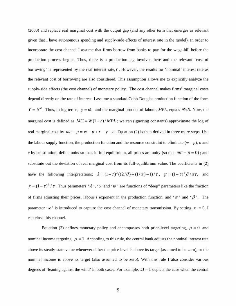
(2000) and replace real marginal cost with the output gap (and any other term that emerges as relevant
given that I have autonomous spending and supply-side effects of interest rate in the model). In order to
incorporate the cost channel I assume that firms borrow from banks to pay for the wage-bill before the
production process begins. Thus, there is a production lag involved here and the relevant ‘cost of
borrowing’ is represented by the real interest rate, r . However, the results for ‘nominal’ interest rate as
the relevant cost of borrowing are also considered. This assumption allows me to explicitly analyze the
supply-side effects (the cost channel) of monetary policy. The cost channel makes firms’ marginal costs
depend directly on the rate of interest. I assume a standard Cobb-Douglas production function of the form
.θNY = Thus, in log terms, ny θ= and the marginal product of labour, MPL, equals θY/N. Now, the
marginal cost is defined as MPLrWMC /)1( += ; we can (ignoring constants) approximate the log of
real marginal cost by .nyrpwpmc +−+−=− Equation (2) is then derived in three more steps. Use
the labour supply function, the production function and the resource constraint to eliminate (w – p), n and
c by substitution; define units so that, in full equilibrium, all prices are unity (so that )0=− pcm ; and
substitute out the deviation of real marginal cost from its full-equilibrium value. The coefficients in (2)
have the following interpretations: ταθτλ /)1)/1()/2(()1( 2 −+−= , ,/)1( 2 ατβτψ −= and
ττγ /)1( 2−= . Thus parameters ‘λ ’, ‘γ ’and ‘ψ ’ are functions of “deep” parameters like the fraction
of firms adjusting their prices, labour’s exponent in the production function, and ‘α ’ and ‘ β ’. The
parameter ‘κ ’ is introduced to capture the cost channel of monetary transmission. By setting κ = 0, I
can close this channel.
Equation (3) defines monetary policy and encompasses both price-level targeting, 0=µ and
nominal income targeting, 1=µ . According to this rule, the central bank adjusts the nominal interest rate
above its steady-state value whenever either the price level is above its target (assumed to be zero), or the
nominal income is above its target (also assumed to be zero). With this rule I also consider various
degrees of ‘leaning against the wind’ in both cases. For example, 1=Ω depicts the case when the central

10
bank conducts monetary policy in a ‘modest’ manner. On the other hand, Ω approaching infinity would
imply that the central bank responds in an ‘aggressive’ manner.
Equation (4) simply captures the relationship between nominal and real interest rate, while
equation (5) depicts the anticipated ongoing cycles in exogenous spending defined by the sine curve.
Since the focus of the paper is on the role of the cost channel in affecting the volatility of output under
alternative monetary policy regimes, the simplest way to introduce fluctuations in output is to assume that
these are caused by exogenous variations in the autonomous spending.
To understand the assumption that the criterion for evaluating the performance of a monetary
regime is its ability to minimize the volatility in real output only and that the two targeting regimes
generate the same outcome regarding long-term inflation, substitute equation (1) in (2) and take the time
derivative. The resulting expression is: ayayp &&&&&&&&& ⎟⎠⎞
⎜⎝⎛+⎟
⎠⎞
⎜⎝⎛−−−=
αβκγ
ακγψλ . Clearly, the policy
parameter µ does not affect the behavior of inflation ( p& ) over time.
Before analyzing the model and discussing the results I briefly talk about the parameter values
that are used in calibrating the model(s) below. Consumption is 60% of the total output, that is, 6.0=α .
This implies that 4.0=β . The other summary coefficients for the baseline Phillips curve relationship can
be calculated by referring to the corresponding values of the ‘deep’ parameters. For example, if labour’s
exponent in the Cobb-Douglas production function is two-thirds ( 67.0=θ ) and the fraction of firms that
are able to adjust their prices once a quarter is one-fourth (Gali and Gertler (1999)), then the
corresponding annual values are: 21.1)75.0/)1)6.0/1()67.0/2(()25.0((*4 2 =−+=λ ,
,22.0)75.0)(6.0/()4.0()25.0((*4 2 ==ψ and 33.0)75.0/)25.0((*4 2 ==γ .10 The parameter δ in
equation (4) is taken as 1.
10 In order to ensure that my results are not dependent on particular values of these parameters, I have considered a
range of other parameter values as well. For example, if we assume that the fraction of firms with sticky prices is 0.85 rather than 0.75 than the values of all summary parameters change accordingly. In particular, they are: 40.0=λ , 07.0=ψ and
11.0=γ . The results, reported in table 2, are not sensitive to these alternative values for various parameters.
11
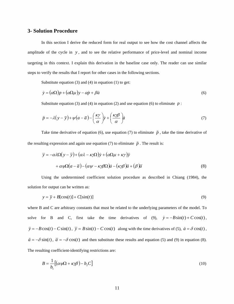
3- Solution Procedure
In this section I derive the reduced form for real output to see how the cost channel affects the
amplitude of the cycle in y , and to see the relative performance of price-level and nominal income
targeting in this context. I explain this derivation in the baseline case only. The reader can use similar
steps to verify the results that I report for other cases in the following sections.
Substitute equation (3) and (4) in equation (1) to get:
( ) ( ) apypy &&& βαµαα +−Ω+Ω= (6)
Substitute equation (3) and (4) in equation (2) and use equation (6) to eliminate p :
( ) ( ) ayaayyp &&&& ⎟⎠⎞
⎜⎝⎛+⎟
⎠⎞
⎜⎝⎛−−+−−=
ακγβ
ακγψλ (7)
Take time derivative of equation (6), use equation (7) to eliminate p&& , take the time derivative of
the resulting expression and again use equation (7) to eliminate p&& . The result is:
( ) ( ) ( )yyyyy &&&&&& κγµακγαλαλ +Ω+Ω−+−Ω−=
( ) ( ) ( ) ( )aaaaa &&&&&& βκγβκγβαψαψ +−Ω−−−Ω+ (8)
Using the undetermined coefficient solution procedure as described in Chiang (1984), the
solution for output can be written as:
)][sin()][cos( tCtByy ++= (9)
where B and C are arbitrary constants that must be related to the underlying parameters of the model. To
solve for B and C, first take the time derivatives of (9), )cos()sin( tCtBy +−=& ,
)sin()cos( tCtBy −−=&& , )cos()sin( tCtBy −=&&& along with the time derivatives of (5), )cos(ta δ=& ,
)sin(ta δ−=&& , )cos(ta δ−=&&& and then substitute these results and equation (5) and (9) in equation (8).
The resulting coefficient-identifying restrictions are:
( )[ ]Cbb
B 21
1−+Ω= κγβαψ (10)
12
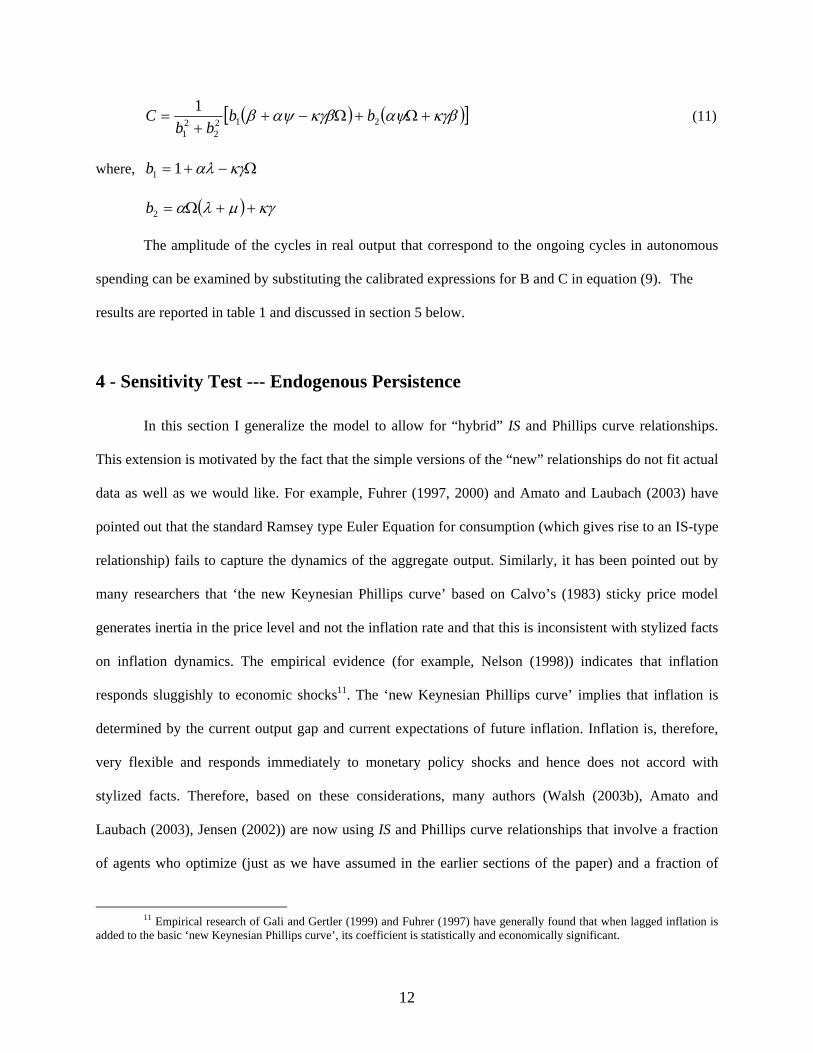
( ) ( )[ ]κγβαψκγβαψβ +Ω+Ω−++
= 2122
21
1 bbbb
C (11)
where, Ω−+= κγαλ11b
( ) κγµλα ++Ω=2b
The amplitude of the cycles in real output that correspond to the ongoing cycles in autonomous
spending can be examined by substituting the calibrated expressions for B and C in equation (9). The
results are reported in table 1 and discussed in section 5 below.
4 - Sensitivity Test --- Endogenous Persistence
In this section I generalize the model to allow for “hybrid” IS and Phillips curve relationships.
This extension is motivated by the fact that the simple versions of the “new” relationships do not fit actual
data as well as we would like. For example, Fuhrer (1997, 2000) and Amato and Laubach (2003) have
pointed out that the standard Ramsey type Euler Equation for consumption (which gives rise to an IS-type
relationship) fails to capture the dynamics of the aggregate output. Similarly, it has been pointed out by
many researchers that ‘the new Keynesian Phillips curve’ based on Calvo’s (1983) sticky price model
generates inertia in the price level and not the inflation rate and that this is inconsistent with stylized facts
on inflation dynamics. The empirical evidence (for example, Nelson (1998)) indicates that inflation
responds sluggishly to economic shocks11. The ‘new Keynesian Phillips curve’ implies that inflation is
determined by the current output gap and current expectations of future inflation. Inflation is, therefore,
very flexible and responds immediately to monetary policy shocks and hence does not accord with
stylized facts. Therefore, based on these considerations, many authors (Walsh (2003b), Amato and
Laubach (2003), Jensen (2002)) are now using IS and Phillips curve relationships that involve a fraction
of agents who optimize (just as we have assumed in the earlier sections of the paper) and a fraction of
11 Empirical research of Gali and Gertler (1999) and Fuhrer (1997) have generally found that when lagged inflation is
added to the basic ‘new Keynesian Phillips curve’, its coefficient is statistically and economically significant.
13
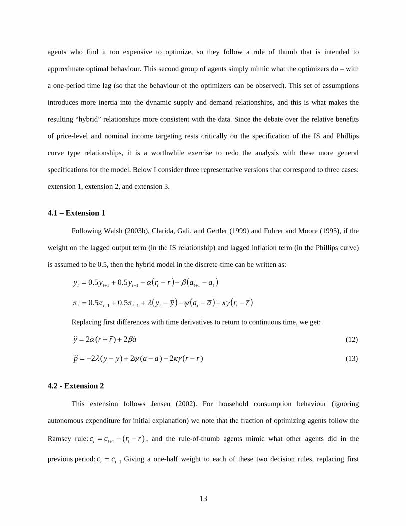
agents who find it too expensive to optimize, so they follow a rule of thumb that is intended to
approximate optimal behaviour. This second group of agents simply mimic what the optimizers do – with
a one-period time lag (so that the behaviour of the optimizers can be observed). This set of assumptions
introduces more inertia into the dynamic supply and demand relationships, and this is what makes the
resulting “hybrid” relationships more consistent with the data. Since the debate over the relative benefits
of price-level and nominal income targeting rests critically on the specification of the IS and Phillips
curve type relationships, it is a worthwhile exercise to redo the analysis with these more general
specifications for the model. Below I consider three representative versions that correspond to three cases:
extension 1, extension 2, and extension 3.
4.1 – Extension 1
Following Walsh (2003b), Clarida, Gali, and Gertler (1999) and Fuhrer and Moore (1995), if the
weight on the lagged output term (in the IS relationship) and lagged inflation term (in the Phillips curve)
is assumed to be 0.5, then the hybrid model in the discrete-time can be written as:
( ) ( )tttttt aarryyy −−−−+= +−+ 111 5.05.0 βα
( ) ( ) ( )rraayy tttttt −+−−−++= −+ κγψλπππ 11 5.05.0
Replacing first differences with time derivatives to return to continuous time, we get:
arry &&& βα 2)(2 +−= (12)
)(2)(2)(2 rraayyp −−−+−−= κγψλ&&& (13)
4.2 - Extension 2
This extension follows Jensen (2002). For household consumption behaviour (ignoring
autonomous expenditure for initial explanation) we note that the fraction of optimizing agents follow the
Ramsey rule: )(1 rrcc ttt −−= + , and the rule-of-thumb agents mimic what other agents did in the
previous period: 1−= tt cc .Giving a one-half weight to each of these two decision rules, replacing first
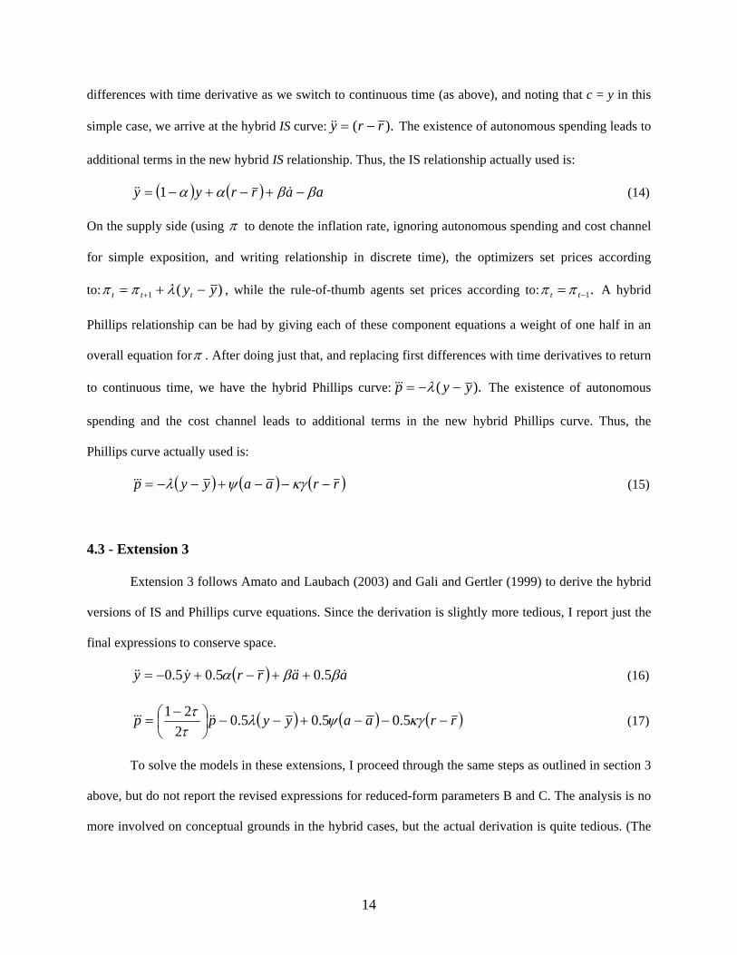
14
differences with time derivative as we switch to continuous time (as above), and noting that c = y in this
simple case, we arrive at the hybrid IS curve: ).( rry −=&& The existence of autonomous spending leads to
additional terms in the new hybrid IS relationship. Thus, the IS relationship actually used is:
( ) ( ) aarryy ββαα −+−+−= &&& 1 (14)
On the supply side (using π to denote the inflation rate, ignoring autonomous spending and cost channel
for simple exposition, and writing relationship in discrete time), the optimizers set prices according
to: )(1 yyttt −+= + λππ , while the rule-of-thumb agents set prices according to: .1−= tt ππ A hybrid
Phillips relationship can be had by giving each of these component equations a weight of one half in an
overall equation forπ . After doing just that, and replacing first differences with time derivatives to return
to continuous time, we have the hybrid Phillips curve: ).( yyp −−= λ&&& The existence of autonomous
spending and the cost channel leads to additional terms in the new hybrid Phillips curve. Thus, the
Phillips curve actually used is:
( ) ( ) ( )rraayyp −−−+−−= κγψλ&&& (15)
4.3 - Extension 3
Extension 3 follows Amato and Laubach (2003) and Gali and Gertler (1999) to derive the hybrid
versions of IS and Phillips curve equations. Since the derivation is slightly more tedious, I report just the
final expressions to conserve space.
( ) aarryy &&&&&& ββα 5.05.05.0 ++−+−= (16)
( ) ( ) ( )rraayypp −−−+−−⎟⎠⎞
⎜⎝⎛ −
= κγψλττ 5.05.05.0
221
&&&&& (17)
To solve the models in these extensions, I proceed through the same steps as outlined in section 3
above, but do not report the revised expressions for reduced-form parameters B and C. The analysis is no
more involved on conceptual grounds in the hybrid cases, but the actual derivation is quite tedious. (The

15
analogue of equation (8) is a fifth-order differential equation in these cases, so many time derivatives of
the trial solution need to be substituted in.)
5 - Results
The results corresponding to baseline parameter values for all four models (the baseline model
and three extensions) with and without the cost channel for both policies (price-level targeting and
nominal income targeting) are reported in table 1. The table also reports both ‘modest’ and ‘aggressive’
policy reactions. In all cases the peaks and troughs in the cycle for output are almost exactly in phase with
those for the cycle in autonomous spending.
The first main result is that in a baseline ‘new Keynesian’ model, nominal income targeting
performs better as compared to price-level targeting in terms of reducing the volatility of real output in
the face of ongoing demand shocks whether cost channel is operating or not or policy response is
moderate or aggressive. Nominal income targeting allows the monetary policy to adjust to offset direct
disturbances to aggregate demand and indirect disturbance to aggregate supply via the cost channel. For
example, in case of an adverse demand shock (corresponding to the trough in the cycle for real output due
to the downward cycle in autonomous spending) that would cause both real output and prices to go below
target, policymakers would ease monetary policy that would push nominal income (the product of real
income and prices) towards target and keep the volatility of nominal income to a minimum. In the
presence of the cost channel, this ease in the monetary policy would lead to favorable supply side
movements as well that would result in rising real output and falling price levels. This could pose a
dilemma if central bank is pursuing price level targeting. The central bank would have to manipulate the
aggregate demand by a large magnitude that would ensure the achievement of the original level of prices
at the cost of an increased volatility in output. On the other hand, with nominal income targeting it would
adjust aggregate demand just enough to reach a targeted level of nominal income with slightly lower level
of prices and slightly higher level of output. The volatility in real output would definitely be lower
16
compared to the price-level targeting case. Since the metric used to evaluate the performance of a
targeting regime is the minimization of real output volatility, nominal income targeting is preferred to
price-level targeting.
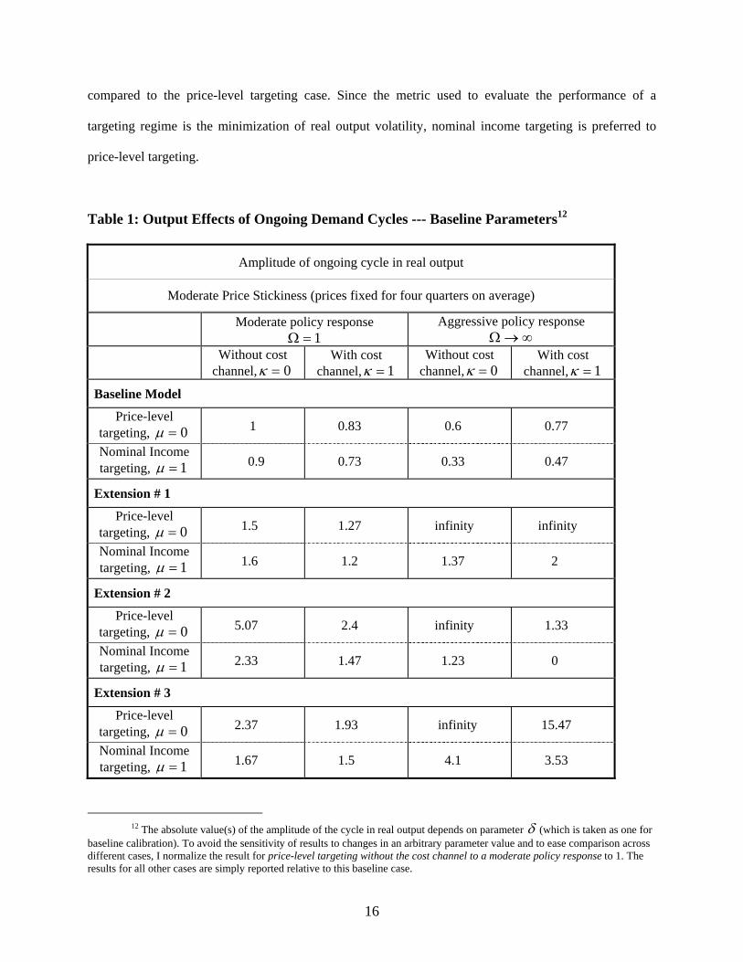
Table 1: Output Effects of Ongoing Demand Cycles --- Baseline Parameters12
Amplitude of ongoing cycle in real output
Moderate Price Stickiness (prices fixed for four quarters on average)
Moderate policy response 1=Ω
Aggressive policy response ∞→Ω
Without cost channel, 0=κ
With cost channel, 1=κ
Without cost channel, 0=κ
With cost channel, 1=κ
Baseline Model
Price-level targeting, 0=µ 1 0.83 0.6 0.77
Nominal Income targeting, 1=µ 0.9 0.73 0.33 0.47
Extension # 1
Price-level targeting, 0=µ 1.5 1.27 infinity infinity
Nominal Income targeting, 1=µ 1.6 1.2 1.37 2
Extension # 2
Price-level targeting, 0=µ 5.07 2.4 infinity 1.33
Nominal Income targeting, 1=µ 2.33 1.47 1.23 0
Extension # 3
Price-level targeting, 0=µ 2.37 1.93 infinity 15.47
Nominal Income targeting, 1=µ 1.67 1.5 4.1 3.53
12 The absolute value(s) of the amplitude of the cycle in real output depends on parameter δ (which is taken as one for
baseline calibration). To avoid the sensitivity of results to changes in an arbitrary parameter value and to ease comparison across different cases, I normalize the result for price-level targeting without the cost channel to a moderate policy response to 1. The results for all other cases are simply reported relative to this baseline case.

17
The result regarding the effects of the cost channel in the baseline case is quite interesting and
somewhat surprising. In the case of ‘moderate policy response’ the volatility of real output goes down in
the presence of the cost channel (in both targeting regimes), while it increases in the case of ‘aggressive
policy response’. Conceptually, this result is quite similar to the one reported by Clarida, Gali and Gertler
(1999) (Result 2, page 1673) for optimal inflation targeting. They call for a gradual convergence of
inflation to its target over time and report that extreme inflation targeting --- adjusting policy to
immediately reach an inflation target --- is optimal only if cost push inflation is absent and there is no
concern for output deviations. Since in the model presented the cost channel is a policy-induced cost push
factor affecting inflation and output volatility is the primary criterion to evaluate the effects of alternative
targeting regimes, a parallel can be drawn between the observation made by Clarida, Gali and Gertler
(1999) and the result reported above. More specifically, a moderate policy response would lead to an
‘optimal’ outcome if the cost channel is operating. Similar conflicting views, also noted by Clarida, Gali
and Gertler (1999), regarding the optimal transition path to the target have emerged in the literature.
Goodfriend and King (1997) favour aggressive policy response because cost push considerations are
absent in their paradigm, while Ball (1999) and Svensson (1999b) consider moderate policy responses as
optimal because cost push inflation considerations play an important role in their frameworks.
How robust are these results? Extension 1, 2 and 3 introduce endogenous inflation and output
persistence by following various approaches employed in the literature. For extension 1 with a moderate
policy response, price-level targeting performs slightly better than nominal income targeting in the
absence of cost channel. However, this difference is rather small. In the presence of cost channel, nominal
income targeting leads to slightly better outcome. Further, the volatility of output goes down in either
targeting regime in the presence of cost channel. With an aggressive approach to policy, price-level
targeting is rather dangerous as the volatility in real output approaches infinity whether the cost channel is
operating or not. This result seems consistent with the observation made by Barnett and Engineer (2000):
“….. price-level targeting is desirable only for a purely forward looking specification of the Phillips
18
curve”. Nominal income targeting, on the other hand, results in finite and small (compared to moderate
policy response) volatility in real output and, as before, the cost channel increases this volatility.
For extension 2, although the amplitude in real output is rather large but the baseline model
results carry over to this general case with one notable exception: with an aggressive policy response,
price-level targeting implies infinite volatility in real output in the absence of cost channel and not when it
is operating. Thus, introducing backward-looking features does not necessarily imply disastrous results
for price-level targeting; the observation noted above by Barnett and Engineer (2000) cannot be
generalized. The cost channel seems to provide stable solutions. This is an important result and needs to
be researched further. Another somewhat interesting result to note is that the volatility in real output
virtually goes to zero with nominal income targeting with the cost channel and an aggressive policy
response. Moreover, the difference between price-level targeting and nominal income targeting is more
pronounced. Extension 3 confirms the results for extension 2 and thus provides more support for them. As
noted by Clarida, Gali and Gertler (1999), in the presence of endogenous persistence in addition to
affecting the gap between the target variable and its target along the convergence path, policy also affects
the rate of convergence and leads to less favorable trade-off between stabilizing inflation and output.
Thus, a more aggressive response to deviation from the target is required because any gap not eliminated
today will persist into the future. This means that we should expect increases in the volatility in real
output, and indeed this is what we observe in all the extensions considered: the volatility in real output is
larger for models with endogenous persistence compared to the baseline forward-looking models. Lastly,
if we introduce endogenous persistence for only output, that is, re-specify the IS relationship and use the
baseline forward-looking inflation dynamics ---the Phillips curve --- (results not reported), even then
nominal income targeting results in smaller and stable outcomes compared to price-level targeting. This
contradicts the claim made by McCallum (1997) that it is only the specification of the Phillips curve that
is important: “…replacement of the Ball-Svensson Phillips curve with the mentioned alternative (new
Keynesian Phillips curve) results in a model in which both output and inflation are dynamically stable
under nominal income targeting whether or not the IS relationship is re-specified”.
19
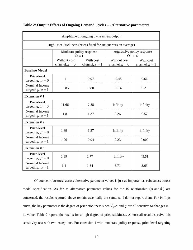
Table 2: Output Effects of Ongoing Demand Cycles --- Alternative parameters
Amplitude of ongoing cycle in real output
High Price Stickiness (prices fixed for six quarters on average)
Moderate policy response 1=Ω
Aggressive policy response ∞→Ω
Without cost channel, 0=κ
With cost channel, 1=κ
Without cost channel, 0=κ
With cost channel, 1=κ
Baseline Model
Price-level targeting, 0=µ 1 0.97 0.48 0.66
Nominal Income targeting, 1=µ 0.85 0.80 0.14 0.2
Extension # 1
Price-level targeting, 0=µ 11.66 2.88 infinity infinity
Nominal Income targeting, 1=µ 1.8 1.37 0.26 0.57
Extension # 2
Price-level targeting, 0=µ 1.69 1.37 infinity infinity
Nominal Income targeting, 1=µ 1.06 0.94 0.23 0.009
Extension # 3
Price-level targeting, 0=µ 1.89 1.77 infinity 45.51
Nominal Income targeting, 1=µ 1.4 1.34 3.71 3.63
Of course, robustness across alternative parameter values is just as important as robustness across
model specification. As far as alternative parameter values for the IS relationship (α and β ) are
concerned, the results reported above remain essentially the same, so I do not report them. For Phillips
curve, the key parameter is the degree of price stickiness since ψλ, and γ are all sensitive to changes in
its value. Table 2 reports the results for a high degree of price stickiness. Almost all results survive this
sensitivity test with two exceptions. For extension 1 with moderate policy response, price-level targeting

20
performs significantly worse than nominal income targeting without the cost channel. For extension 2
with aggressive policy response, price-level targeting implies infinite volatility in output even in the
presence of cost channel. Another sensitivity test considered is the inclusion of nominal interest rate
(rather than real interest rate) in the Phillips curve to capture the cost channel. Since virtually all general
conclusions survive this sensitivity testing, I do not include additional tables here.
What broad conclusions can we draw from the above discussion? First, nominal income targeting
is superior to price-level targeting in all most all cases regardless of the cost channel and alternative
degrees of policy responses. Second, output volatility goes down due to the cost channel in case of a
moderate policy response, while it increases for aggressive policy. Third, in case of an aggressive
response to policy for models with endogenous persistence, price-level targeting leads to infinite volatility
in output without the cost channel. With cost channel it results in stable outcomes.
6- Concluding Remarks
This paper studied the main developments in the macroeconomic theory regarding the
specifications for the aggregate demand and aggregate supply side of the model and the transmission
mechanism of monetary policy in the context of two rule-based monetary policy regimes: price-level
targeting and nominal income targeting. Comparing the results presented in the series of macroeconomic
models indicate that analysing both the traditional and the cost channel of monetary policy in one unified
framework has been worthwhile. They confirm the results of earlier theoretical and empirical research on
the potency of supply side effects of monetary policy (the cost channel) in effecting the real economy.
Moreover, the paper also finds strong support for a case in favour of nominal income targeting when
compared with price-level targeting as it keeps the volatility of real output low. There is a growing
literature that studies and compares the performance of these targeting regimes and a consensus has not
been reached yet. Thus, the results of this paper can be considered as an addition to this debate. An
important point in this regard is that the specification of both the demand side and the supply side of the
model are crucial while analysing various monetary policy targeting regimes.
21
However, I agree with McCallum (1997) when he concluded while comparing the performance of
inflation targeting and nominal income targeting: “This demonstration does not establish that nominal
income targeting is preferable to inflation targeting or to other rules for monetary policy. To reach such a
conclusion would require an extensive combination of theoretical and empirical analyses, conducted in a
manner that gives due emphasis to the principle of robustness to model specification, plus attention to
concerns involving policy transparency and communication with the public”. The point of this paper was
not to attempt any such ambitious undertaking. However, the results can be considered as a small step in
that direction.
References
Amato, J., and T. Laubach (2003), “Rule-of-Thumb Behavior and Monetary Policy”, European Economic Review 47, pp. 791-831. Ball, L. (1999), “Efficient Rules for Monetary Policy”, International Finance, Vol. 2, No. 1, pp. 63-83. Barnett, R., and M. Engineer (2000), “When is Price-Level Targeting a Good Idea?”, in “Price Stability and the Long-Run Target for Monetary Policy”, Proceedings of a seminar held by the Bank of Canada, June. Barth, M., and V. Ramey (2001), “The Cost Channel of Monetary Transmission”, NBER Working Paper No. 7675. Bean, C., (1983), “Targeting Nominal Income: An Appraisal”, The Economic Journal 93, pp. 806 – 819. Calvo, G., (1983), “Staggered Prices in a Utility Maximizing Framework”, Journal of Monetary Economics, pp. 383-398. Chiang, A., (1984), “Fundamental Methods of Mathematical Economics”, McGraw-Hill Book Company, Third Edition. Christiano, L., and M. Eichenbaum, (1992), “Liquidity Effects and the Monetary Transmission Mechanism”, American Economic Review 82, pp. 346 – 353. Christiano, L., M. Eichenbaum and C. Evans (1997), “Sticky Price and Limited Participation Models of Money: A Comparison”, European Economic Review 41, pp – 1201-1249. Clarida, R., Gali, J., and M. Gertler (1999), “The Science of Monetary Policy: A New Keynesian Perspective”, Journal of Economic Literature, pp. 1661-1707. Dennis, R., (2001), “Inflation Expectations and the Stability Properties of Nominal GDP Targeting”, The Economic Journal 111, pp. 103 – 113.
22
Dittmar, R., and W. Gavin (2000), “What Do New Phillips Curve Imply for Price Level Targeting?”, Federal Reserve Bank of St. Louis Review, March/April Issue. Dittmar, R., Gavin, W., and F. Kydland, (1999), “The Inflation-Output Variability Trade-off and Price-level Targets”, Federal Reserve Bank of St. Louis Review, January/February Issue. Dixit, A., and J. Siglitz, (1977), “Monopolistic Competition and Optimum Product Diversity”, American Economic Review 67, pp. 297 – 308. Fischer, S., (1994), “Modern Central Banking”, in Capie, F., Goodhart, C., Fischer, S., and N. Schnadt (eds.), “The Future of Central Banking”, Cambridge University Press. Fuhrer, J.C., (1997), “Towards a Compact, Empirically Verified Rational Expectations Model for Monetary Policy Analysis”, Carnegie-Rochester Conference Series on Public Policy 47, pp. 197 – 230. Fuhrer, J. (2000), “Habit Formation in Consumption and its Implications for Monetary Policy Models”, American Economic Review 90, pp. 367-390. Fuhrer, J. and G. Moore (1995), “Inflation Persistence”, Quarterly Journal of Economics, 110, No. 1, pp. 127-159. Gali, J., and M. Gertler, (1999), “Inflation Dynamics: A Structural Econometric Analysis”, Journal of Monetary Economics 44, pp. 195 – 222. Goodfriend, M. and R. G. King (1997), “The New Noeclassical Synthesis and the Role of Monetary Policy”, NBER Macroeconomics Annual, pp. 231 – 283. Haldane, A., and C. Salmon, (1995), “Three Issues on Inflation Targets”, in Haldane, A., (ed.), “Targeting Inflation”, A conference of the central banks on the use of inflation targets, Bank of England. Hall, R., and G. Mankiw, (1994), “Nominal Income Targeting”, in Mankiw, G., (ed.), “Monetary Policy”, NBER Studies in Business Cycles, Vol. 29. Jensen, H., (2002), “Targeting Nominal Income Growth or Inflation”, American Economic Review, Vol. 94, No. 4, pp. 928 – 956. Kashyap, A., and J. Stein, (1994), “Monetary Policy and Bank Lending”, in Mankiw, G., (ed.), “Monetary Policy”, NBER Studies in Business Cycles, Vol. 29. Kiley, M., (1998), “Monetary Policy under Neoclassical and New-Keynesian Phillips Curves, with an Application to Price Level and Inflation Targeting”, Finance and Economics discussion paper, 98-27, Federal Reserve Board. King, R.G. (2000), “The New IS-LM Model: Language, Logic, and Limits”, Economic Quarterly, Federal Reserve Bank of Richmond, Vol. 86, No.3, pp. 45 – 103. Lam, J-P, and W. Scarth (2002), “Monetary Policy and Built-in Stability”, Review of International Economics, Vol. 10, No. 3, pp. 469-482.
23
McCallum, B., (1997), “The Alleged Instability of Nominal Income Targeting”, Reserve Bank of New Zealand, G-97/6. McCallum, B, and E. Nelson (1999), “An Optimizing IS-LM Specification for Monetary Policy and Business Cycle Analysis”, Journal of Money, Credit and Banking, pp. 296-315. Mishkin, F. (2000), “Issues in Inflation Targeting”, in “Price Stability and the Long-Run Target for Monetary Policy”, Proceedings of a seminar held by the Bank of Canada, June. Mitchell, D.W, (1984), “Macro Effects of Interest Sensitive Aggregate Supply”, Journal of Macroeconomics 6, pp. 43-56. Myatt, A., (1985), “The Adverse Supply-side Effects of High Interest Rates and Procyclical Real Wage Movements”, Journal of Macroeconomics 7, pp. 237-246. Myatt, A. and William Scarth (2003), “Is Policy Perversity Consistent With Keynesian Business Cycles?”, Journal of Macroeconomics 25, pp. 351-365. Nelson, E., (1998), “Sluggish Inflation and Optimizing Models of the Business Cycle”, Journal of Monetary Economics, Vol. 42, No. 2, pp. 303-322. Rudebusch, G., (2002), “Assessing Nominal Income Rules for Monetary Policy with Model and Data Uncertainty”, The Economic Journal, pp. 402-432. Sargent, T.J., and N. Wallace, (1976), “Rational Expectations and the Theory of Economic Policy”, Journal of Monetary Economics 2, pp. 169 – 183. Svensson, L., (1999a), “Price Level Targeting vs. Inflation Targeting: A Free Lunch?”, Journal of Money, Credit and Banking, pp. 277-295. Svensson, Lars (1999b), “Inflation Targeting: Some Extensions”, Scandinavian Journal of Economics, Vol. 101, Issue 3, pp. 607 – 654. Vestin, D., (2003), “Price-level Targeting versus Inflation Targeting”, forthcoming in the Journal of Monetary Economics, February. Walsh, C., (2003a), “Monetary Theory and Policy”, Second Edition, The MIT Press. Walsh, Carl (2003b), “Speed Limit Policies: The Output Gap and Optimal Monetary Policy”, American Economic Review 93(1), March, pp. 265 – 278. Walsh, C., and F. Ravenna, (2006), “Optimal Monetary Policy with the Cost Channel”, Journal of Monetary Economics, Vol. 53. West, K., (1986), “Targeting Nominal Income: A Note”, The Economic Journal 96, pp. 1077–1083.