Embed Size (px)
Citation preview
MPRAMunich Personal RePEc Archive
Is Rentier Capitalism That Bad? Rent,Efficiency and Inequality Dynamics
Mohamed Mabrouk
Ecole Superieure de Statistique et d’Analyse de l’Information deTunis
24 September 2017
Online at https://mpra.ub.uni-muenchen.de/81748/MPRA Paper No. 81748, posted 2 October 2017 21:05 UTC

Is Rentier Capitalism That Bad?Rent, Efficiency and Inequality Dynamics
Version September 24, 2017
Mohamed Mabrouk1
Abstract
The current economic context shows a tendency to inequality and rather
weak growth. Rent-seeking behavior is often blamed for that. The purpose of
this paper is to analyze the consequences, on the accumulation trajectory, of
the existence of a rent levied by the rich on the poor. The model is inspired
by the articles [Stiglitz 1969], [Schilcht 1975] and [Bourguignon 1981]. In par-
ticular, convex saving is used. We seek to see to what extent the introduction
of a rent may call into question the Pareto-superiority of inequality proved by
[Bourguignon 1981] or alter the risk of decline highlighted in [Mabrouk 2016].
Within the limits of the assumptions of the model and of the numerical simula-
tions carried out, we arrive at interesting and rather unexpected observations.
Namely, a moderate rent levied by the rich on the poor may not only allow a
Pareto-improvement of the economy and prevent the risk of decline, but also,
it may unlock the economy from under-accumulation trap even if initial capital
endowment is insufficient. The disadvantages of such a rent for the poor are
felt only if the economy approaches or exceeds the golden rule where the net
marginal productivity of capital is zero.
1 Introduction
The current economic context shows a tendency to an increase in the income
of the rich to the detriment of the poor2. [Jacobs 2016] and [Stiglitz 2015 b]
suggest that this increase in high incomes stems from rents with no clear coun-
terpart in terms of output, such as rents due to market power, cronyism, or
position rents due to the possession of irreplaceable assets such as well-situated
buildings3.
This situation is not in line with the neoclassical theory of income distribu-
tion according to marginal productivities that predicts that every factor earns
a competitive income according to what it adds to domestic production. Would
deviation from that theory have a negative impact on growth and economic
efficiency? Although in the public debate the answer to this question tends to
be positive, it is useful to look at it in more detail at the theoretical level4 .
1Ecole Supérieure de Statistique et d’Analyse de l’Information (Tunis), 6 rue des métiers,
Charguia 2, Tunis, Tunisia; tel: 21655368471; email: [email protected] See for example: [Oxfam report “Even It Up” 2014].3For more precision on the meaning of the word "rent" in this context, see [Stiglitz 2015 b]
page 7.4 [Murphy-Shleifer-Vishny 1993] analyzed the effect of "rent-seeking" behavior in terms of
efficiency and economic growth. However, their approach differs from ours because, on the
one hand, it considers rent-seeking as a productive activity in its own right, and on the other
it does not place the question of rent in a dynamic perspective of capital accumulation.
1

The purpose of this paper is to analyze, within the framework of a simple
neoclassical model, the consequences of the existence of a rent levied by the
rich class on the competitive income of the poor class as set by the neoclassical
theory of income distribution according to marginal productivities. This is
done in a demonetized context, without uncertainty nor technical change, and
taking into account the difference in saving behavior according to the level of
income. The model is inspired by the articles [Stiglitz 1969], [Schilcht 1975]
and [Bourguignon 1981]. The economy has two production factors: capital and
labor, a production function with constant returns to scale, and an individual
marginal propensity to save increasing with income. Individuals are assumed
to be similar in all respects except for their membership in a given social class.
This differentiates them only by their initial capital endowments and the rent
received or paid.
Ignoring differences between individuals in terms of skills, saving behaviors
and random events that could differentiate them, aims to focus on the im-
personal aspect of inequalities dynamics. In this context, it appears that the
assumption of a marginal propensity to save increasing with income (i.e. a con-
vex saving function) is crucial for the emergence of distinct and stable social
classes. Indeed, [Stiglitz 1969] showed that a linear saving function leads to the
convergence of classes. Even when considering a pseudo-convex saving func-
tion, where the marginal propensity to save passes discontinuously from 0 to a
constant positive value when income increases, [Stiglitz 2015 a] shows that the
only stable configuration remains a single social class. By extending the work
of [Stiglitz 1969] to the case of convex savings, [Schilcht 1975] showed that one
can get two stable classes. [Bourguignon 1981] then showed that the equilibrium
with two classes Pareto-dominates the egalitarian equilibrium.
Unlike [Stiglitz 2015 a] which focuses on inequality in itself and its causes,
it should be noted that the present work is in the spirit of [Bourguignon 1981],
where the main concern is efficiency rather than inequality, and where egalitar-
ian equilibrium is a poverty-trap from which one must escape. In this context,
one seeks to see to what extent the introduction of a rent levied by the rich class
on the income of the poor class may call into question the Pareto-superiority of
the unequal configuration proved by [Bourguignon 1981]. We also want to see to
what extent the introduction of such a rent alters the risk of decline highlighted
in [Mabrouk 2016].
After introducing the model and the assumptions in section 2, sections 3, 4
and 5 attempt to prepare the mathematical groundwork of the general model in
order to show how rent modifies the curves that govern equilibrium under the
conditions imposed in section 2. From section 6 on, since general calculations
lack exploitable explicit formulas, we take a numerical example to follow the
evolution of equilibria according to rent levels. This makes it possible to arrive at
interesting, rather unexpected observations on the way in which rent influences
the economic trajectory and the type of equilibrium. It should be noted that,
although the parameters of the simulations are chosen at reasonable levels, these
simulations do not pretend to have an empirical value.
Sections 7 and 8 study the equilibrium response to the variation of two
2

essential parameters: the proportion of rich and the social propensity to save.
Charts are often used to base arguments. Charts without numerical values
represent only the shapes of the curves and are drawn by hand. Those with
numerical values are computed and plotted by computer.
2 Model and assumptions
The same assumption and notations as [Mabrouk 2016] are used, except some
specified below.
Individual savings are assumed to depend on income according to the func-
tion () where is the income of the individual concerned. is convex,
increasing, twice differentiable on ]0+∞[ and checks (0) = 0 0(0) 0 and
lim→∞
0() = 1. Denote the inverse function of . We have 0 1 00 0 and
lim 0() =→∞
1 The per capita production function is () where is the average
capital per capita. is increasing, concave, twice differentiable on ]0+∞[ andchecks (0) = 0 The capital undergoes depreciation at a rate per unit of time
and capital. ∗ is the per capita capital of the golden-rule defined by 0(∗) = .
The society is composed of two classes: the poor, in proportion 1 and the
rich in proportion 2 = 1− 1. We assume 2 1.
The following two conditions guarantee that we do not deviate too much
from the case where the saving function is linear and where there exists a unique
stable egalitarian equilibrium with non-zero production:
Condition 1 0(0) 0(0)
Condition 2 There is a unique b such that 0 ³b´− 0³b´ = 0
These conditions reduce the generality of this paper, but they allow to lighten
the analysis while giving an idea of what can happen when the saving function
is convex.
Proposition 3 shows that conditions 1 and 2 imply that the equation ()− () = 0 has a unique solution 0 0. This value is in fact the capital of the
egalitarian equilibrium of the economy under consideration.
Like in [Bourguignon 1981], assume that:
0 ∗ (1)
The economic interpretation of assumption (1) is that the poor class does
not generate enough savings to achieve maximum efficiency of the economy.
Instead of the usual neoclassical assumption that labor and capital are paid
according to their respective marginal productivities, it is assumed that the
wealthy class gains a rent in addition to its competitive income. The rent
is levied by the rich class on the competitive income of the poor class.
3

By normalizing the size of the population to 1, per capita income in the rich
class is:
()− 0() + 20() +
2
Per capita income in the poor class is:
()− 0() + 10()−
1
where 1 2 are respectively per capita capital in the poor class and per capita
capital in the rich class.
The dynamics of the economy are then characterized by the following differ-
ential system:
·1 =
∙() + (1 − ) 0()−
1
¸− 1
·2 =
∙() + (2 − ) 0() +
2
¸− 2
= 11 + 22
By using the inverse function of , the equilibrium must satisfy the fol-
lowing system:
() + (1 − ) 0()−
1= (1) (2)
() + (2 − ) 0() +
2= (2)
= 11 + 22
Denote (1) and (2) the locus of the points in the space ( ) defined
respectively by the first and second equations of the system (2).
In the following, the curves (1) and (2) are constructed with the help of
graphic arguments.
3 The relationship between 1and 2 at equi-
librium
3.1 Plotting the curve (2) :
By deriving the two equations of (1) and (2) with respect to , we obtain an
expression which gives the derivative of with respect to on (1) or (2):
[ 0()− 0()] = ”()( − ) (3)
Denote () the locus of the points in the plane ( ) checking:
0()− 0() = 0
4
As explained in [Bourguignon 1981], () is increasing, lies in the half-plane
( ∗) and admits the straight line ( = ∗) as a vertical asymptote.
Proposition 3 There is a unique 0 0 such that () − () = 0 and we
have b 0 and 0 (0)− 0 (0) 0
Proof: Define the function () = () − () We have (0) = 0 and
0 () = 0 ()− 0 () By condition 1, 0 (0) 0. Moreover, since 0(∗) =
there is 0 such that for sufficiently large, we have 0() 0 Thus, when tends towards +∞ we have 0() 0− 0()→ 0− 0Taking accountof conditions 1 and 2 and since 0 is continuous, we deduce that 0 is positiveonh0bh, zero at b and negative on ib+∞h Thus is increasing on h0bh and
decreasing onib+∞h The properties concerning 0 arise therefrom QED
As stated above, 0 is the equilibrium reached with a single social class, i.e.
the egalitarian equilibrium. By virtue of the inequality 0 (0)− 0 (0) 0,the egalitarian equilibrium 0 is stable.
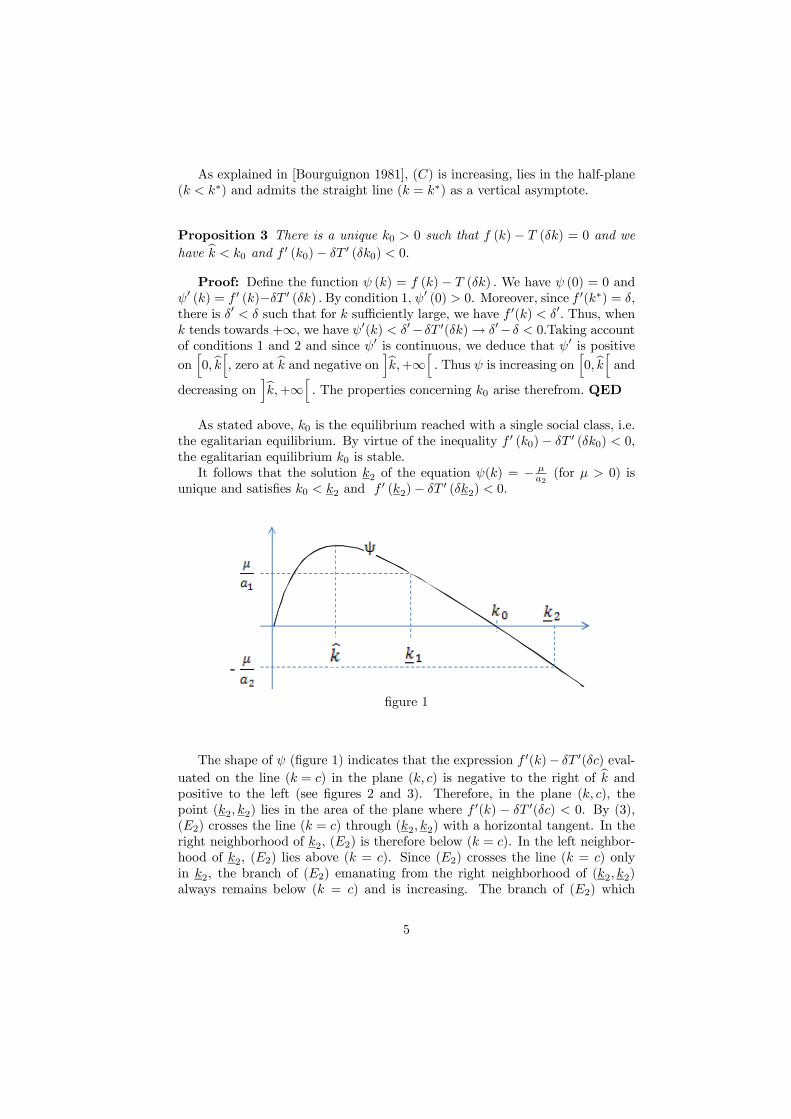
It follows that the solution 2 of the equation () = − 2(for 0) is
unique and satisfies 0 2 and 0 (2)− 0 (2) 0
‐
figure 1
The shape of (figure 1) indicates that the expression 0()− 0() eval-uated on the line ( = ) in the plane ( ) is negative to the right of b andpositive to the left (see figures 2 and 3). Therefore, in the plane ( ), the
point (2 2) lies in the area of the plane where 0() − 0() 0. By (3),
(2) crosses the line ( = ) through (2 2) with a horizontal tangent. In the
right neighborhood of 2 (2) is therefore below ( = ). In the left neighbor-
hood of 2, (2) lies above ( = ). Since (2) crosses the line ( = ) only
in 2, the branch of (2) emanating from the right neighborhood of (2 2)
always remains below ( = ) and is increasing. The branch of (2) which
5
emanates from the left neighborhood of (2 2) always remains above ( = )
and decreases until it encounters () as the case may be.
Proposition 4 In contrast to the curve () in [Mabrouk 2016], the introduc-
tion of causes two cases to occur: (2) intersects the vertical ( = ∗) or doesnot intersect it.
Proof: Consider the expression = () − −h(∗)− ∗ +
2
i
The value of at = 0 is negative. The derivative of with respect to
is: ( 0() − 1) 0. is then increasing as a function of . Its max-
imum is max = lim→∞ [ ()− ] −h(∗)− ∗ +
2
i Denote 0 =
2 (lim→∞ [ ()− ]− [(∗)− ∗]). Assumption (1) implies (∗) 0
i.e. (∗)− (∗) 0 By evaluating the expression ()−−[(∗)− ∗]in = ∗, we get (∗) − (∗). We thus have 0
2= max [ ()− ] −
[(∗)− ∗] ≥ (∗)− (∗) 0 Thus 0 0
It follows that if 0, then the expression ()−−h(∗)− ∗ +
2
itakes the value 0 for some ∗ in ]0+∞[ Thus the curve (2) intersects thevertical ( = ∗) at (∗ ∗) If ≥ 0, then there is no
∗ such that (∗ ∗) ∈(2) QED
Case 1: ≥ 0
Proposition 5 (2) is entirely to the right of the vertical ( = ∗) and thisvertical is an asymptote to (2)
Proof: For a given , assume there exists ≥ 0 such that () + ( −) 0()+
2= (). We thus have
2= ()− ()− (−) 0() ≥ 0
2=
lim→∞ [ ()− ]−[(∗)− ∗]. Hence, ()− 0() ≥ max [ ()− ]−[((∗)− ∗ 0(∗))− (()− 0())]. If → ∗+, this inequality can be writ-ten ()− ≥ max [ ()− ]− , where is as small as one wants. This
shows that tends to +∞ since the maximum of () − is reached for
→ +∞. Therefore the vertical ( = ∗) is an asymptote to (2).If → ∗−, for all ≥ 0 we have
()− 0() ≥ [ ()− ]− [((∗)− ∗ 0(∗))− (()− 0())]
Take 0 = − positive and close to 0. Then take as close as necessary
to ∗− so that the quantity [((∗)− ∗ 0(∗))− (()− 0())] be negligible
in comparison with () − (). This gives the inequality − 0() ≥ () − () ≥ 0. For 0 sufficiently close to 0+, the latter inequality gives − 0() ≥ 0, which is impossible for ∗. We deduce that the curve (2)does not pass in the left neighborhood of ∗. Therefore, the curve (2) does notpass in the area [0 ∗] because, assuming the opposite and using (3), we wouldget step by step to the left neighborhood of ∗ QED
6

Remark 6 It is useful for the following to observe that since (2) does not
intersect the area [0 ∗] when ≥ 0, for capital to equal ∗ at equilibrium it
is necessary to have 0
figure 2
Case 2: 0This case is similar to the case addressed in [Bourguignon 1981]. The branch
of (2) which emanates from the left neighborhood of 2 intersects () at a point
denoted (2 2). According to (3), the tangent to (2) at point (2 2) is
vertical. (2) becomes increasing as soon as it passes above () at (2 2).
When increases from 2, this branch can not intersect again () because it
should do so with a vertical slope, which is not possible since () does not have
any vertical tangent. Therefore it remains above (). Note that 0(2) = 0(2) implies 0(2) . So 2 ∗ When tends to ∗ from the left, the
branch of (2) above ( = ) admits a vertical asymptote like ()
figure 3
7

We now give some properties that help to see the changes that take place
when varies.
We have the following inequalities b 2 2 2 and 2 ∗
Proposition 7 lim→0− 2 = ∗
Proof: Since 2 = −1( 2), 2 varies continuously with respect to . We
know that for = 0, we have 2 ∗. Therefore, when → 0−, we havelim→0− 2 ∗.Therefore, when → 0− (2) is decreasing between 2 and ∗, so
2 ∗. It is now sufficient to see that lim→0− ∗ = +∞ to deduce that
lim→0− 2 = +∞, and, being on the curve (), to deduce that lim→0− 2 →∗. Indeed, → 0− can be written as:2 = [ (
∗)− ∗]−[(∗)− ∗]→ 20 = lim→∞
[ ()− ]−[(∗)− ∗]
which entails lim→0− ∗ = +∞ QED
Proposition 8 2 is increasing as a function of
Proof: Differentiate (2)+(2−2) 0(2)+ 2= (2) with respect
to along the curve (). We get: 02 =1
2(2−2) 00(2) 0QED
Proposition 9 2 is increasing as a function of and lim→+∞ 2 = +∞
Proof: The function () has an asymptotic direction with a slope strictly
less than and the function () has an asymptotic direction with slope .
Therefore lim→+∞ () = () − () = −∞. Equation (2) = − 2
implies lim→+∞ 2 = +∞. By differentiating the expression (2) = − 2
with respect to , we get: 0(2)02 = − 1
2. But 0(2) 0. So 02 0
QED
It is useful for the following to see the solutions of the second equation of
(2) in another way. Denote by 2() the expression () + ( − ) 0() +2, considering as a parameter and as a variable; and denote by () the
expression (). The function is concave and its derivative satisfies 0 1.Therefore the function is concave and its derivative satisfies 0 .
We are now in the plane (2) In the case 0, 2 and are tangent
at the point 2 for = 2. If increases, according to figure 3, we obtain
two intersections 2 and 2 so long as the asymptotic slope of , which is ,
is less than the slope of 2, which is 0() i.e. as long as ∗. As soon as
exceeds ∗, the line 2 flips as shown in figure 4. The point 2 is rejected at
infinity and the intersection becomes only 2.
8

Y
X2
c
X2(0)
X2 ,Y
ci2 cs2
figure 4
If ≥ 0 and if ≤ ∗, there is no intersection between and 2. If
∗, the intersection is limited to a single point.
3.2 Plotting the curve (1) :
Figure 1 shows that under the assumption:
1 = 1³b´ (4)
equation () = 1has two solutions, the largest of which, denoted 1, is
greater than bWe shall limit ourselves to the cases where condition 4 is satisfied.5
We are interested only in the solution of the first equation of system (2) which
is greater than b. Indeed, (2) lies entirely on the right of b and therefore therecan not be a pair (1 2) that verifies the first two equations of (2) if ≤ b.To the right of b, the pair (1 1) is solution of the first equation of (2). The
curve (1) is constructed in the plane ( ) starting from the point (1 1) in
the same way as (2).
Denote 1() the expression () + (− ) 0() − 1. The representation
of 1() is added to figure 4 by observing that the two straight lines 1() and
2() are parallel and that 1(0) 2(0)
5For the proposed numerical application, we will see that this condition is not limiting
since the value of 1 is more than 44%. It goes far beyond the other critical values of that
our analysis reveals.
If 1 the curve (1) would divide into two branches, one above the line ( = ) and
the other beneath. The interesting branch is that which is below, as in the case ≤ 1. We
will not deal here with the case ≥ 1
9
Y X1
X2(0)
X1, X2 ,Y
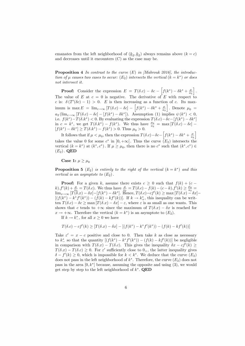
ci2 cs2ci1 cs1
X1(0)
X2
figure 5
Therefore, as long as 1(0) 0 and 2 intersects at two points, 1
intersects at two non-zero points 1 and 1 such that 1 2 and 1
2. In the plane ( ), the upper branch of (1) will be above the upper
branch of (2) and the lower branch of (1) will lie below the lower branch of
(2). Condition 1(0) 0 amounts to () − 0() − 1
0. Denote by
() = () − 0() is increasing on [0+∞[ and (0) = 0 (because the
concavity of and (0) = 0 gives 0 () (), hence lim→0 0 () = 0)
Condition 1(0) 0 is equivalent to: () 1.
In order to confirm the construction of the curve (1), carried out similarly
to (2), the following two properties are proved:
Proposition 10 Condition 1(0) 0 is satisfied as long as bProof: For b we have 0 () 0 thus 0 () 0 () Moreover, by
concavity of and (0) = 0, the function ()− 0 () is increasing in
and is zero for = 0 Thus ()− 0 () 0 for ∈ ]0+∞[ To sum up:
0 () 0 () () This gives () = ()− () ()− 0 () = () for b For ∈ ib 1i, we then get () () ≥ (1) =
1 And
for 1, we get () (1) (1) =1 We have proven that if b
then () 1. QED
Proposition 11 The first equation of (2) does not admit a solution in = b(a fortiori the second equation - see figure 5).
10

Proof: Suppose there is 1 such that (b) + (1 − b) 0(b)− 1= (1)
Subtract (b) from the two sides of the latter equation. It gives:µ(b)− (b)−
1
¶+ (1 − b) 0(b) = (1)− (b)
But³(b)− (b)−
1
´ 0 Thus (1−b) 0(b) (1)− (b) Replace
0(b) by 0(b) It gives: (1 − b) 0(b) (1) − (b) The latterinequality is impossible since () is concave. QED
Thus, by decreasing towards b from 1, the intersection between the line
1 and passes from 2 points to 0 point, knowing that the abscissas of the
points of intersection, when they exist, are in ]0+∞[. Thus 1 "detaches"
from before reaches b. By continuity, this necessarily occurs when 1 and
become tangent for some value of denoted 1.
We thus have b 1 1 1
Figure 1 shows that lim→11 =
b. We deduce lim→11 = b . There-
fore, 1 being the image of 1 on the curve (), we also have lim→11 = b.
Since is decreasing onhb+∞h and (1) =
1
0 = (0), we have
1 0 ∗. This allows to construct the curve (1) starting from the point
1 as we have done for (2) when 0
We easily establish the following formulas which show that 1 and 1 are
decreasing as functions of :
01 = −1
1 (1 − 1) 00 (1) 0
01 =1
10(1)
0
Figure 6 gives the shapes of the curves (1) and (2) for 0 and ≥ 0 :
11
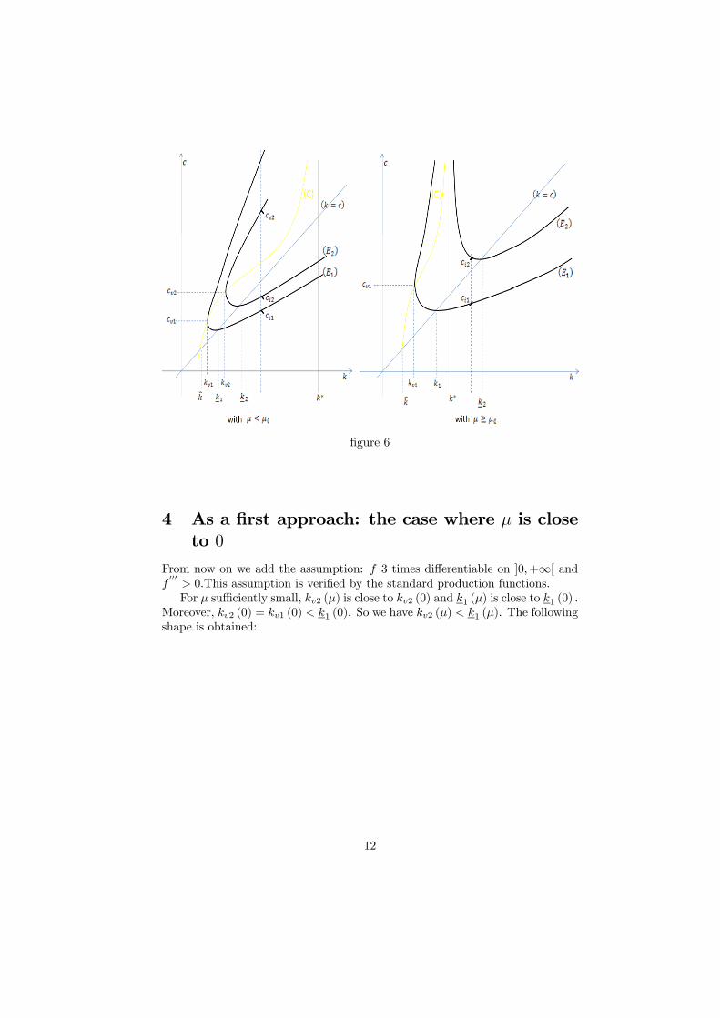
figure 6
4 As a first approach: the case where is close
to 0
From now on we add the assumption: 3 times differentiable on ]0+∞[ and000 0This assumption is verified by the standard production functions.
For sufficiently small, 2 () is close to 2 (0) and 1 () is close to 1 (0)
Moreover, 2 (0) = 1 (0) 1 (0). So we have 2 () 1 (). The following
shape is obtained:
12

figure 7
For ∈ [1 2] define the function () by the equality = () 2()+
(1− ())1()
() is continuous. It is positive on ]1 2], zero at 1 and it takes the
value 1 at 2. From now on, it is assumed that the system (2) is smooth enough
for the functions 1() and 2() to be differentiable.
Proposition 12 () is increasing on [1 2]
Proof: The assumption 000 0 is used here The denominator of the expres-
sion of () is decreasing on [1 2] since 2 is decreasing and 1 is increasing
on this interval. Let us show that − 1() is increasing as a function of .
This is equivalent to showing that 1− 1
0. Using equation (3), we get:
1− 1
= 1− ”()( − 1)
0()− 0(1)
We have to show that”()(−1)
0()− 0(1) 1. Observe that below the curve
() the quantity 0(1) − 0() is positive. We thus have to show that
−”()( − 1) 0(1) − 0(). Since 1 b, we have 0 (1) 0, thus
0(1) 0(1). Therefore, we shall have attained our objective if we showthat −”()( − 1) 0(1) − 0() This last inequality follows from the
assumption 000 0 which implies that 0 is convex. QED
13

The properties " () increasing on [1 2]", " (1) = 0" and " (2) =
1" show that for 2 ∈ [0 1] there exists a unique 00 such that (00) = 2. The
triplet (00 1(00) 2(
00)) is therefore a solution of system (2).
If → 0 then 1 → 0 and 2 → 0. The system (2) can be linearized
around 0 for close to 0. Denote:
− 0 =
1 − 0 =
2 − 0 =
The first equation of system (2) becomes
(0) + 0(0) + ( − ) 0(0)−
1' 0(0)
thus
'
10(0)
Similarly, we establish the approximation
' −
20(0)
and
' 0Since 0(0) 0 we have 0 and 0 Average capital at equilibrium
is almost equal to the egalitarian equilibrium capital 0. But the poor class is
worse off and the rich class is better off.
We are now interested in the possible equilibria on the lower branch of (1)
and the upper branch of (2). These equilibria can be seen as the result
of deformations following the introduction of a rent, of inegalitarian equilib-
ria in the case without rent studied in [Schilcht 1975], [Bourguignon 1981] and
[Mabrouk 2016].
For ∈ [1 ∗[ define the function () by the equality = () 2()+
(1− ())1()
In the same way as in [Mabrouk 2016], we see that () is zero in 1,
positive on ]1 ∗[ and lim→∗ () = 0. Consequently () admits a
maximum on ]1 ∗[. This maximum is given by the resolution of the system of
6 unknowns 1 21
2
and and the 6 equations given in [Mabrouk 2016],
page 80.
However, unlike [Mabrouk 2016], depends on 1 and 2 because the curves
(1) and (2) depend on 1 and 2.
The same kind of reasoning as in [Bourguignon 1981] shows that equilibria
on the lower branch of (1) and the upper branch of (2) occur in peers and that
the equilibrium with the highest value of capital is stable. If is close enough
14
to 0, this equilibrium is close to the stable Pareto-dominant equilibrium of
[Bourguignon 1981]. Hence, it is Pareto-superior to the egalitarian equilibrium
0. This does not fundamentally alter the conclusions obtained in the case
without rent.
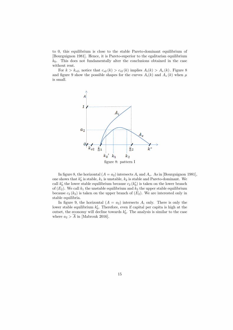
For 2, notice that 2 () 2 () implies () () Figure 8
and figure 9 show the possible shapes for the curves () and () when
is small
figure 8: pattern I
In figure 8, the horizontal ( = 2) intersects and. As in [Bourguignon 1981],
one shows that 00 is stable, 1 is unstable, 2 is stable and Pareto-dominant. Wecall 00 the lower stable equilibrium because 2 (
00) is taken on the lower branch
of (2). We call 1 the unstable equilibrium and 2 the upper stable equilibrium
because 2 (2) is taken on the upper branch of (2). We are interested only in
stable equilibria.
In figure 9, the horizontal ( = 2) intersects only. There is only the
lower stable equilibrium 00. Therefore, even if capital per capita is high at theoutset, the economy will decline towards 00. The analysis is similar to the casewhere 2 in [Mabrouk 2016].
15
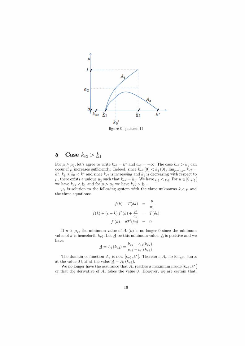
figure 9: pattern II
5 Case 2 1
For ≥ 0 let’s agree to write 2 = ∗ and 2 = +∞ The case 2 1 can
occur if increases sufficiently. Indeed, since 2 (0) 1 (0) lim→0− 2 =∗, 1 ≤ 0 ∗ and since 2 is increasing and 1 is decreasing with respect to, there exists a unique 2 such that 2 = 1. We have 2 0 For ∈ [0 2[we have 2 1 and for 2 we have 2 1.
2 is solution to the following system with the three unknowns and
the three equations:
()− () =
1
() + (− ) 0 () +
2= ()
0()− 0() = 0
If 2, the minimum value of () is no longer 0 since the minimum
value of is henceforth 2 Let be this minimum value is positive and we
have:
= (2) =2 − 1(2)
2 − 1(2)
The domain of function is now [2 ∗[. Therefore, no longer starts
at the value 0 but at the value = (2).
We no longer have the assurance that reaches a maximum inside ]2 ∗[
or that the derivative of takes the value 0. However, we are certain that,
16
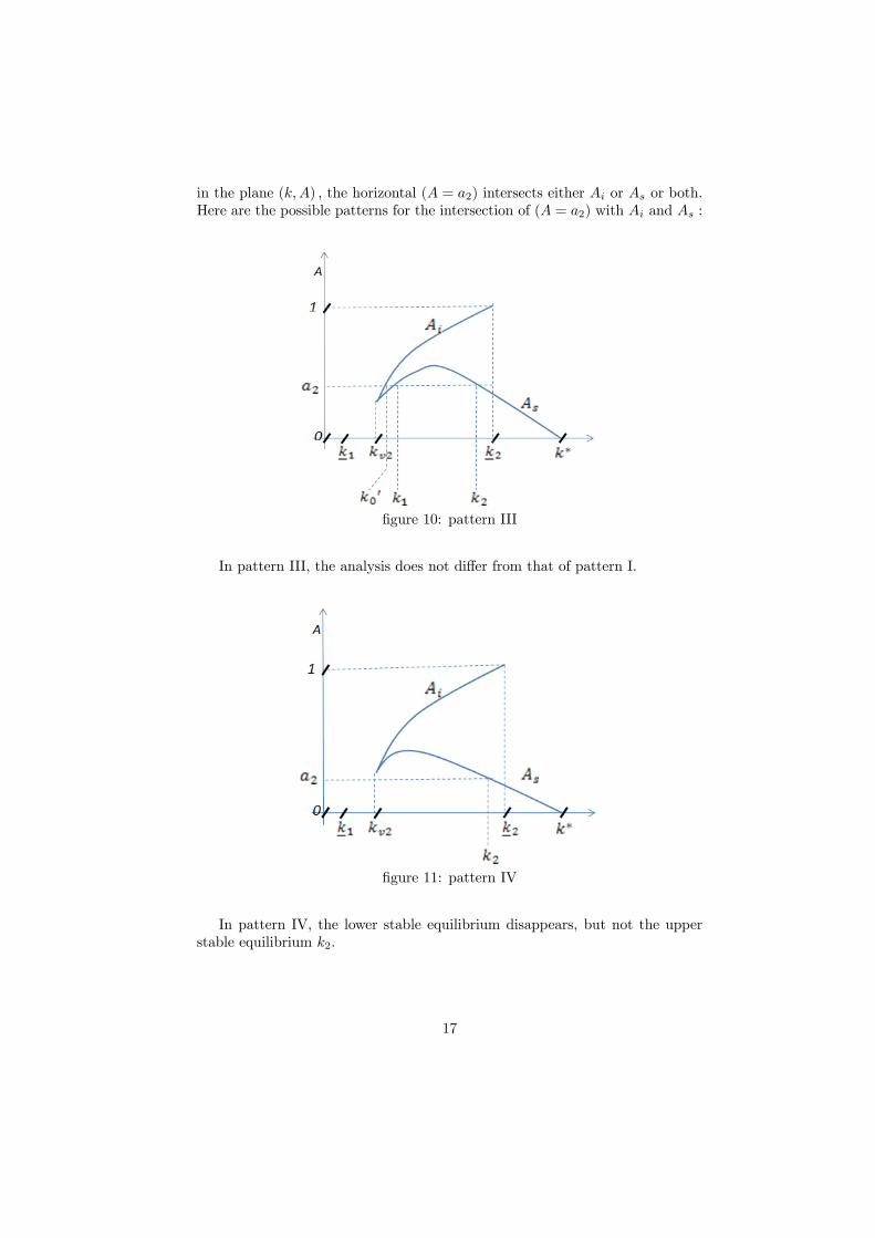
in the plane () the horizontal ( = 2) intersects either or or both
Here are the possible patterns for the intersection of ( = 2) with and :
figure 10: pattern III
In pattern III, the analysis does not differ from that of pattern I.
figure 11: pattern IV
In pattern IV, the lower stable equilibrium disappears, but not the upper
stable equilibrium 2.
17

figure 12: pattern V
In pattern V, there is only equilibrium 00. The position of this equilibriumon should not suggest that the value of
00 is small. It will be seen that
00
reaches high values for sufficiently large.
figure 13: pattern VI
Figure 13 represents when ≥ 0. The curve disappears in this case
because the upper branch of (2) no longer exists when ≥ 0. The analysis
of the equilibrium does not differ from that of pattern V.
Furthermore, () is zero for ∈ [0 2] and positive for ∈ ]2 0[.
Functions and are supposed to be sufficiently smooth for the variables
18

2 2 1(2) to be continuous with respect to . Consequently, () is con-
tinuous with respect to over the interval [0 0[. It has been shown above that
lim→0− 2 → ∗ and lim→0− 2 = +∞. We deduce that lim→0− () =0. For ≥ 0 we agree to write () = 0. If max () 2, we obtain the
following figure:
figure 14
with 3 = inf { () = 2} and 4 = sup { () = 2} If it is not thecase, one moves directly from pattern II to pattern V and then VI. Changing
the saving function may yield max () 2 This is discussed in section 8.
If = 3 or = 4 we obtain an equilibrium which lies at the point of
coordinates (2min) in the plane (). Thus, in the plane ( ), the
corresponding point ( 2) is none other than (2 2) and lies on the curve
()
Remark 13 The above entails 3 ≤ 4 0.
Proposition 14 The derivative with respect to of the net income of the poor
at 2 is zero for = = 3 or 4
Proof: The point ( 2) = (2 2) satisfies the equation of () : 0(2)−
0() = 0. If we add this equation to the 3 equations of the system (2), we ob-
tain 4 equations for the four unknowns 1 2 . By combining the first two
equations of (2), we get:
() = 1 (1) + 2 (2) (5)
For any , the solution ( 1 2) of the system (2) can be considered as
a function ( () 1 () 2 ()) of Differentiate (5) with respect to It
gives: 0()0 = 101
0 (1) + 202
0 (2) Now take again = Re-
place 0() by its value given by the equation of () It gives: 0(2)0 =1
01
0 (1) + 202
0 (2) Now replace 0 by 101 + 2
02. It gives:
0(2)¡1
01 + 2
02
¢= 1
01
0 (1) + 202
0 (2) After rearranging:1
01
0(2) = 101
0 (1) Thus 010(2) = 01
0 (1) Since 1 6= 2we have necessarily 01 = 0 The income of the poor is: ()+(1−) 0()−
1−
19
1 The first equation of (2) allows us to write this income as: (1)−1 Thederivative of this expression with respect to is: ( 0 (1)− 1) 01 = 0QED
The economic interpretations of 3, 4 and proposition 14 will be developed
in the following sections.
6 A numerical example
6.1 General data
We adopt the parameters used in [Mabrouk 2016] 6 . The numerical values are
only intended to highlight the economic phenomena that are being analyzed.
They are chosen at levels supposed to be reasonable. But the question of con-
formity of these numerical values with the reality of a given country is not
considered here not to clutter up this paper. The production function is chosen
in such a way that it gives a gross income normalized to 1 with a capital coef-
ficient of 25 (i.e. (25) ' 1). This makes it possible to interpret the values ofthe rent in terms of percentage of the gross income normalized to 1 considered
as reference income. For example, = 15 ·10−2 is interpreted as a rent of 15%of the reference income.
We take () = 3403 The rate of capital depreciation is 37% The saving
function is constructed to meet the conditions of section 2 and realize savings
rates ranging from 10% to 30% depending on income levels.
The formula chosen is:
() = +1
2(1 + )( − ) +
1−
1 +
s0 +
∙1
2(1 + )( − )
¸2with
= 17105249
= 00301171
= 00677230
0 = 01889504
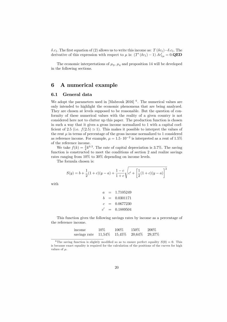
This function gives the following savings rates by income as a percentage of
the reference income
income 10% 100% 150% 200%
savings rate 11,54% 15,45% 20,64% 29,37%
6The saving function is slightly modified so as to ensure perfect equality (0) = 0. This
is because exact equality is required for the calculation of the positions of the curves for high
values of .
20
The proportion of rich is set at 2 = 3% and the proportion of poor at
1 = 97%.
The following results are obtained for 1 and 2, with an error smaller than
10−4:
1 = 4418 · 10−22 = 037 · 10−2
The value 2 = 037·10−2 represents a rent of 037% of the reference income.The value 1 = 4418 ·10−2 represents a rent of 4418% of the reference income.
For 0, we have to compute lim→+∞ [ ()− ]. It turns out that this
limit is equal to
lim→+∞
[ − ()] = −
Thus 0 = 163 · 10−2.Finally, we verify that the assumptions of section 2 are met, in particular
conditions 1 and 2.
6.2 Description of a gradual increase in rent
We examine what happens when varies from 0 to a limit value where the
equilibrium income of the poor is less than the egalitarian income. This value
of will be denoted 6.
We observe the succession of the following patterns: I, III, IV, V.
We thus begin with a situation close to the case without rent. We obtain the
3 equilibria: lower stable equilibrium 00, unstable equilibrium 1, upper stable
equilibrium 2. As mentioned in section 4, as long as is weak the analysis does
not differ much from the case = 0 studied in [Mabrouk 2016]. This means
that if the initial capital is insufficient and the propensity to save of the poor
is low, the economy may find itself locked in the lower stable equilibrium 00,which, as long as one is in pattern I, is Pareto-dominated by the upper stable
equilibrium 2.
For example, for = 007·10−2, the lower stable equilibrium is: (00 1 2) =(652 651 701). The upper stable equilibrium is: (2 1 2) = (1161 715 15767).
7
From = 2 = 037 · 10−2, we proceed to pattern III. The lower stableequilibrium is then: (00 1 2) = (660 645 1146). The upper stable equilib-rium is: (2 1 2) = (1199 717 16778). This new upper stable equilibrium
is better, in the Pareto sense, than the one attained with a lower rent. Thus,
the increase of the rent levied on the income of the poor makes it possible to
7The values of capital are given with an error smaller than 10−2 and the values of rentsare given with an error smaller to 10−4.
21
increase not only the income of the rich but also that of the poor! The under-
lying reason is that rent promotes a better accumulation that improves labor
productivity, which, in turn, improves wages.
If is still increased, it is observed that starting from 3 = 0 4 · 10−2, weproceed to pattern IV where there is no longer lower stable equilibrium. The
risk of falling into poverty8 no longer exists.
It thus appears that an increase in rent not only improves the
economy in the Pareto sense, but also helps to compensate for the
possible lack of initial capital which may otherwise threaten to lock
the economy in poverty.
If we further increase , starting from 4 we proceed to pattern V (figure
12). That is, in the plane () the equilibrium is taken on the curve instead
of the curve . Therefore, in the plane ( ), the equilibrium value of 2 is now
taken on the lower branch of (2). The calculation gives 4 = 150 · 10−2. Theobservation shows that at = 4 the net income of the poor is maximum. This
fact is confirmed by proposition 14. So to speak, 4 is the "pro-poor" capitalist
rent. This remark is not valid for 3 because in this case the upper equilibrium
is not realized at 2.
For the rich, on the other hand, their net income always increases with
within the limits of the interval of the study (figure 21).
For = 4 the unique equilibrium is: (2 1 2) = (1313 719 20499)
From 4 on, the analysis of the equilibrium does not change. The average
capital at equilibrium continues to increase until exceeding the golden-rule cap-
ital ∗. Denote by 5 the value of beyond which the average capital exceeds
∗. So to speak, 5 is the "efficient rent". The calculation gives 5 ' 156·10−2.The observed ranking 3 ≤ 4 5 0 is in accordance with remarks 6 and
13
The crossing of 0 = 163 · 10−2 does not change the equilibrium analysis
and does not have any particular economic significance.
From 6 on, the net equilibrium income of the poor falls below egalitarian
income. The calculation gives 6 ' 1607 · 10−2. This level is significantlyhigher than the pro-poor rent 4 and the efficient rent 5.
The following figures represent the equilibrium positions for each of the fol-
lowing cases: 0 ≤ 2 2 ≤ 3 3 ≤ 4 4 ≤ 0 and 0 ≤
Arrows indicate the movement of the equilibrium when increases
8 I use the terminology "poverty" to describe a state of general under-accumulation.
22

figure 15: 0 ≤ 2 (pattern I )
figure 16: 2 ≤ 3 (pattern III)
23

figure 17: 3 ≤ 4 (pattern IV)
figure 18: 4 ≤ 0 (pattern V)
24
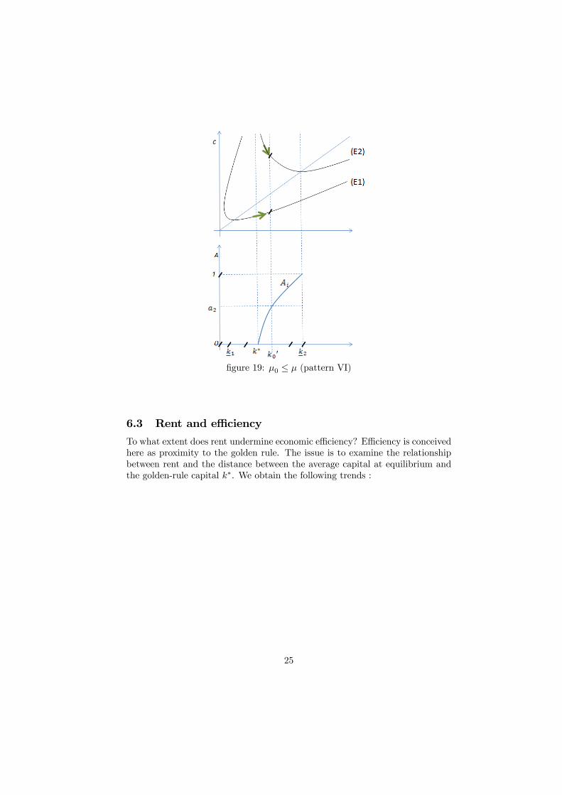
figure 19: 0 ≤ (pattern VI)
6.3 Rent and efficiency
To what extent does rent undermine economic efficiency? Efficiency is conceived
here as proximity to the golden rule. The issue is to examine the relationship
between rent and the distance between the average capital at equilibrium and
the golden-rule capital ∗. We obtain the following trends :
25
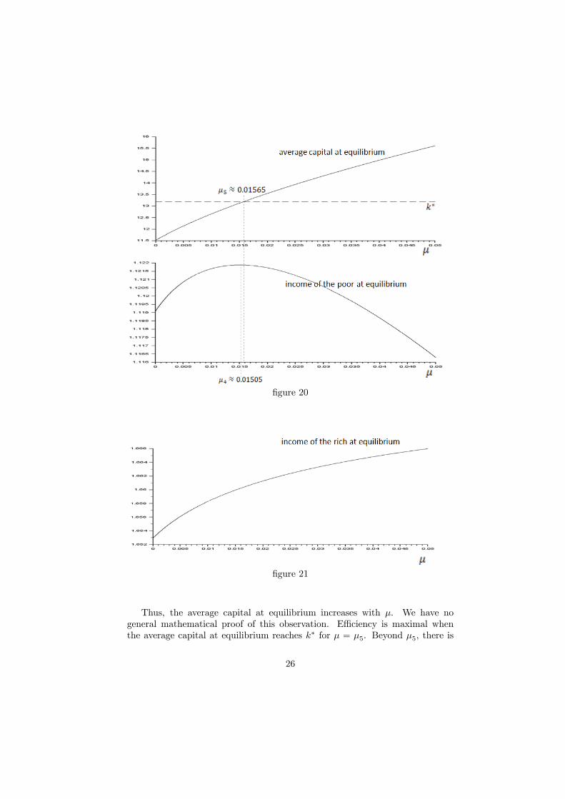
figure 20
figure 21
Thus, the average capital at equilibrium increases with . We have no
general mathematical proof of this observation. Efficiency is maximal when
the average capital at equilibrium reaches ∗ for = 5. Beyond 5, there is
26

overaccumulation of capital. The proximity between 4 and 5 suggests
that it is the poor who bear the cost of overaccumulation because their
income begins to decline while the income of the rich continues to grow. We
also have no general mathematical proof for the proximity between 4 and 5
The plotting of the function () makes it possible to display the val-
ues of 2, 3 and 4, as well as the areas "release from poverty", "Pareto-
improvement" and "declining income of the poor":
figure 22
6.4 Partial release from poverty
As has been shown in [Mabrouk 2016], in the case of a zero rent, if one starts
with too high a proportion of rich, the only equilibrium is the lower stable
equilibrium. Even if the initial capital endowment is high, the economy is
caught in a vicious circle of deaccumulation where savings can no longer cover
the maintenance costs of a capital stock that has become too high. This was
referred to as "Keynesian decline" in [Mabrouk 2016], because of a passage
from [Keynes 1936] describing a decline caused by the conjunction of an excess
of wealth and inequality. In such a case, it is interesting to see what happens
when adding a capitalist rent (i.e. rent to the benefit of the rich).
Take 2 = 55%. In this case, with a zero rent, the value of is calculated
to be 504% (by using the 6 equations given in [Mabrouk 2016], page 80). The
economy declines towards poverty since 2 . If increases, the value of
increases. For = 01 · 10−2 we find = 530%. For = 02 · 10−2 we find
27
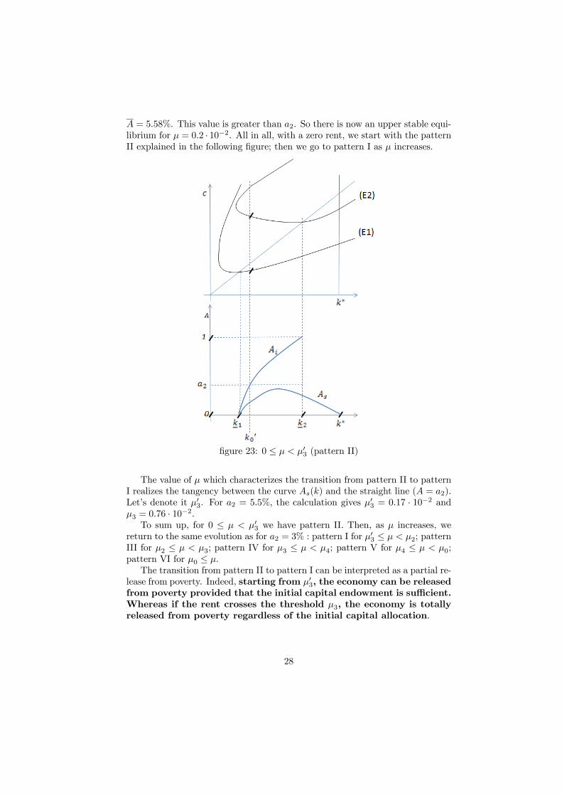
= 558%. This value is greater than 2. So there is now an upper stable equi-
librium for = 02 · 10−2. All in all, with a zero rent, we start with the patternII explained in the following figure; then we go to pattern I as increases.
figure 23: 0 ≤ 03 (pattern II)
The value of which characterizes the transition from pattern II to pattern
I realizes the tangency between the curve () and the straight line ( = 2).
Let’s denote it 03. For 2 = 55% the calculation gives 03 = 017 · 10−2 and3 = 076 · 10−2.To sum up, for 0 ≤ 03 we have pattern II. Then, as increases, we
return to the same evolution as for 2 = 3% : pattern I for 03 ≤ 2; pattern
III for 2 ≤ 3; pattern IV for 3 ≤ 4; pattern V for 4 ≤ 0;
pattern VI for 0 ≤ .
The transition from pattern II to pattern I can be interpreted as a partial re-
lease from poverty. Indeed, starting from 03, the economy can be releasedfrom poverty provided that the initial capital endowment is sufficient.
Whereas if the rent crosses the threshold 3, the economy is totally
released from poverty regardless of the initial capital allocation.
28

figure 24
In conclusion to this section and contrary to immediate intuition, the levying
of a rent by the rich class can play a favorable role for the whole economy,
including for the poor class.
Moreover, the example studied in this subsection shows that the risk of
Keynesian decline can be avoided by means of a rent. Indeed, the rent makes it
possible to meet the needs for the maintenance of capital when savings without
rent cannot any longer cover them.
However, and more in line with immediate intuition, beyond a certain level
of rent (4 ' 150% of reference income when 2 = 3%), the equilibrium incomeof the poor decreases with the increase of capitalist rent.
7 Variation of 2
In the case without rent, when 2 tends to 0 we have seen in [Mabrouk 2016]
that when the savings of the poor are insufficient, the economy tends towards
maximum efficiency whatever the saving function, provided that it is convex. It
29
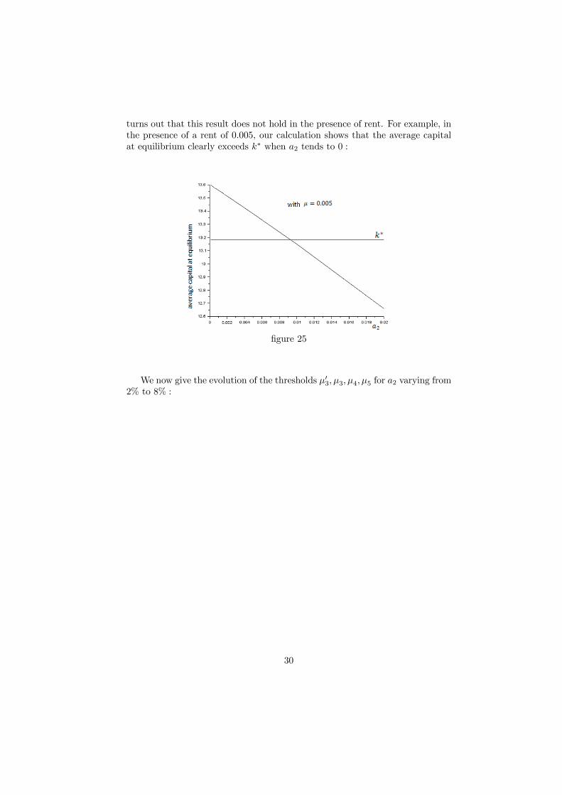
turns out that this result does not hold in the presence of rent. For example, in
the presence of a rent of 0005, our calculation shows that the average capital
at equilibrium clearly exceeds ∗ when 2 tends to 0 :
figure 25
We now give the evolution of the thresholds 03 3 4 5 for 2 varying from2% to 8% :
30

figure 26
We read in figure 26 that for 2 504%, the economy is doomed to poverty
as long as 03 even if the initial capital endowment is high (Keynesiandecline). If is in the interval [03 3[, the economy can be released frompoverty provided that it has enough initial capital. If ≥ 3, the economy is
released from poverty whatever the initial capital.
For 2 ≤ 504%, there is no longer any possibility of Keynesian decline. Theeconomy is condemned to poverty only if the initial capital is insufficient. As
soon as ≥ 3, the economy is released independently of the initial capital.
In the following 3 charts, we represent the average capital at equilibrium,
the net income of the poor at equilibrium and the net income of the rich at
equilibrium as a function of 2, for different values of . These charts show
that for = 01 · 10−2 the Keynesian decline occurs for 2 between 55% and
6%. For = 05 · 10−2 the Keynesian decline occurs for 2 between 65% and
7%. The more one increases , the more one increases the proportion of rich
that the economy is able to bear without falling into decline. This suggests
that rent makes it possible to stabilize the accumulation of capital by
protecting it from the risk of decline that arises when the proportion
of rich becomes high.
31
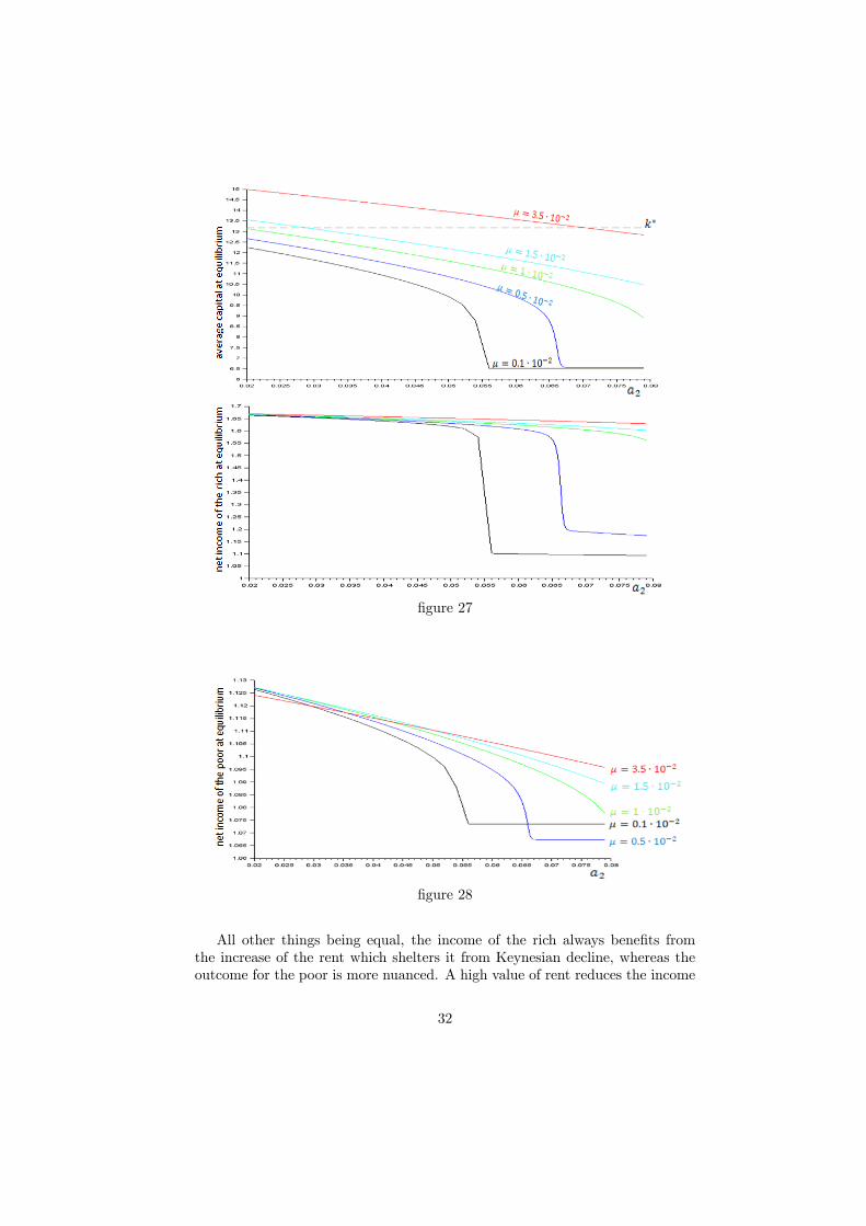
figure 27
figure 28
All other things being equal, the income of the rich always benefits from
the increase of the rent which shelters it from Keynesian decline, whereas the
outcome for the poor is more nuanced. A high value of rent reduces the income
32

of the poor if the proportion of rich is not excessive. The reason is the cost of
overaccumulation that is borne by the poor as seen in subsection 6.3. For the
poor, if the proportion of rich is low, it is better to have a low capitalist rent.
But if the proportion of the rich is high, it is better to accept a higher capitalist
rent in order to rule out the risk of Keynesian decline.
What happens now if, for each value of 2, the capitalist rent is fixed at its
pro-poor level 4? The following 2 charts show that everyone wins:
figure 29
Note that the value of 4 in figure 29 changes for each value of 2.
8 Variation of the social propensity to save
As in [Mabrouk 2016], the saving function is modified by introducing a coeffi-
cient in the following way:
() =1
()
The variation of the coefficient represents the variation of the general
willingness to save of society. If increases, this willingness increases and vice
33

versa. For this reason, we call the "social propensity to save".9
If we represent the curve () of figure 22 for several values of and with
2 = 3%, the following figure is obtained:
figure 30
The two intersections of () with the horizontal ( = 2 = 3%) are 3 and
4. If approachese by lower values, 3 and 4 approach one another. If
exceeds e, there is no intersection. This means that if exceeds e, there is nolonger any risk of Keynesian decline.
We now give the evolution of the thresholds 3 03 4 and 5 for varying
from 08 to 125 (with 2 = 3%).
9As in [Mabrouk 2016], we draw the reader’s attention to the fact that the variation of
the coefficient alone can not represent all the possibilities of modifying the profile of the
willingness to save. For example, one can conceive of an increase in the willingness to save
among the poor and simultaneously a decrease in this willingness among the rich. Such a
modification is not captured by the parameter and is not considered in the present study.
34

figure 31
For ≥ e, the optimal capitalist rent for the poor is 0. This means thatwhen the social propensity to save is high, a rent, even small, is harmful to the
poor.
However, we can have ≥ e and 5 0. Thus, while harmful to the poor
for ≥ e, rent can help improve economic efficiency if it remains below 5.
The curve 5 () intersects the x-axis at a pointee. Beyond ee, the economy
is overaccumulated whatever the value of the rent. By taking a zero rent, we
see thatee is the solution of the equation [ (∗)] = ∗. In other words,
the egalitarian equilibrium capital 0
µee¶ is equal to the golden-rule capital
∗. It can be deduced that when the social propensity to save is very high, therent no longer offers any social advantage. A strong social propensity to save is
able to put the economy in the trajectory of a stable accumulation without the
help of rent. The only effect of rent would then be to enriching the rich at the
expense of the poor. It is only in this case that the effect of rent corresponds to
immediate intuition: an unjust and unproductive extortion.
We are now interested with the variation of 0 according to . The value of
0 as a function of is given by the following formula:
0 = 2
³lim→∞
[()− ]− [(∗)− ∗]´
= 2
µ1
lim→∞
[ ()− ]− [(∗)− ∗]
35
For = 08, we obtain 0 = 289 · 10−2. For = 12, we obtain 0 =
079 · 10−2. It is observed that for any value of , 0 is greater than 5. This is
consistent with remark 6
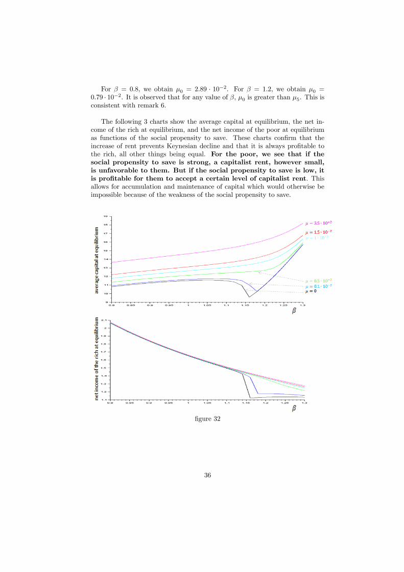
The following 3 charts show the average capital at equilibrium, the net in-
come of the rich at equilibrium, and the net income of the poor at equilibrium
as functions of the social propensity to save. These charts confirm that the
increase of rent prevents Keynesian decline and that it is always profitable to
the rich, all other things being equal. For the poor, we see that if the
social propensity to save is strong, a capitalist rent, however small,
is unfavorable to them. But if the social propensity to save is low, it
is profitable for them to accept a certain level of capitalist rent. This
allows for accumulation and maintenance of capital which would otherwise be
impossible because of the weakness of the social propensity to save.
figure 32
36
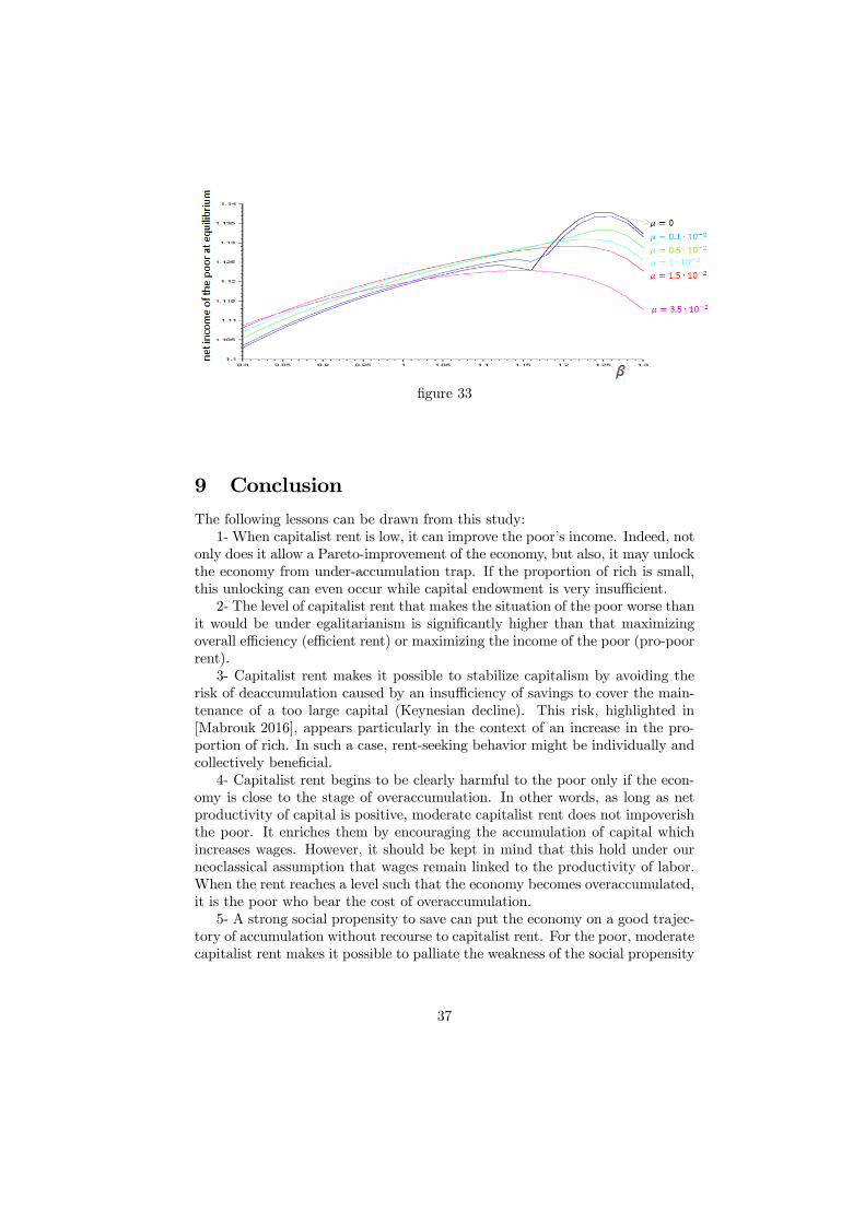
figure 33
9 Conclusion
The following lessons can be drawn from this study:
1- When capitalist rent is low, it can improve the poor’s income. Indeed, not
only does it allow a Pareto-improvement of the economy, but also, it may unlock
the economy from under-accumulation trap. If the proportion of rich is small,
this unlocking can even occur while capital endowment is very insufficient.
2- The level of capitalist rent that makes the situation of the poor worse than
it would be under egalitarianism is significantly higher than that maximizing
overall efficiency (efficient rent) or maximizing the income of the poor (pro-poor
rent).
3- Capitalist rent makes it possible to stabilize capitalism by avoiding the
risk of deaccumulation caused by an insufficiency of savings to cover the main-
tenance of a too large capital (Keynesian decline). This risk, highlighted in
[Mabrouk 2016], appears particularly in the context of an increase in the pro-
portion of rich. In such a case, rent-seeking behavior might be individually and
collectively beneficial.
4- Capitalist rent begins to be clearly harmful to the poor only if the econ-
omy is close to the stage of overaccumulation. In other words, as long as net
productivity of capital is positive, moderate capitalist rent does not impoverish
the poor. It enriches them by encouraging the accumulation of capital which
increases wages. However, it should be kept in mind that this hold under our
neoclassical assumption that wages remain linked to the productivity of labor.
When the rent reaches a level such that the economy becomes overaccumulated,
it is the poor who bear the cost of overaccumulation.
5- A strong social propensity to save can put the economy on a good trajec-
tory of accumulation without recourse to capitalist rent. For the poor, moderate
capitalist rent makes it possible to palliate the weakness of the social propensity
37
to save. But it becomes detrimental to them if the social propensity to save is
strong.
These lessons rely of course on the simplifying assumptions of our model: no
money, only one good, no technical progress, no uncertainty, and most impor-
tantly the assumption of a rigid saving behavior not related to the position in
the accumulation trajectory. The main difference between this assumption and
the standard intertemporal optimization model is the persistence of a strong
propensity to save for high incomes in periods when greater consumption would
have been socially preferable. Nevertheless, we believe that this type of behav-
ior, although rigid, is more realistic than intertemporal optimization because
the latter does not capture the game between capitalists who, at a certain stage
of accumulation, are under the threat of deaccumulation because of the decline
in the productivity of capital. It is likely that this threat contributes to a high
propensity to save at the wrong time. There is much to gain from studying this
issue in the context of a dynamic game.
References
[Bourguignon 1981] François Bourguignon, Pareto-Superiority
of Unegalitarian Equilibria in Stiglitz’
Model of Wealth Distribution With Con-
vex Saving Function, Econometrica, vol. 49,
N◦6, Nov. 1981
[Dynan-Skinner-Zeldes 2004] Karen E. Dynan, Jonathan Skinner,
Stephen P. Zeldes, Do The Rich Save
More?, Journal of Political Economy, vol
112, n◦2, 397-444, 2004
[Jacobs 2016] Didier Jacobs, Extreme Wealth Is Not Mer-
ited, Oxfam Discussion Paper, Nov. 2016
[Keynes 1936] Keynes J.M. (1936), "General Theory
of Employment, Interest and Money",
http://cas.umkc.edu/economics/ peo-
ple/facultypages/kregel/courses/econ645/
winter2011/generaltheory.pdf
[Mabrouk 2016] Mohamed Mabrouk, The Paradox Of
Thrift In An Inegalitarian Neoclassical
Economy, Business And Economic Hori-
zons, vol. 12, issue 3, Dec. 2016, DOI:
http://dx.doi.org/10.15208/beh.2016.07
38
[Murphy-Shleifer-Vishny 1993] Kevin M. Murphy, Andrei Shleifer, Robert
W. Vishny, Why Is Rent-Seeking So Costly
To Growth? The American Economic Re-
view, 83(2): 409—14, 1993
[Oxfam report “Even It Up” 2014] Oxfam report, “Even It Up”, 2014,
http://oxfamilibrary.openrepository.com/
oxfam/bitstream/10546/333012/43/cr-
even-it-up-extreme-inequality-291014-
en.pdf
[Schilcht 1975] Ekkehart Schilcht, A Neoclassical Theory
of Wealth Distribution, Jahrbücher für Na-
tionalökonomie und Statistik, 189, 78-96,
1975
[Stiglitz 2015 a] Joseph Stiglitz, New Theoretical Per-
spectives On The Distribution Of
Income And Wealth Among Individu-
als: Part II: Equilibrium Wealth Dis-
tributions, National Bureau Of Eco-
nomic Research, WP 21190, May 2015,
http://www.nber.org/papers/w21190
[Stiglitz 2015 b] Joseph Stiglitz, Inequality And Economic
Growth, The Political Quaterly, Dec. 2015
, DOI: 10.1111/1467-923X.12237
[Stiglitz 1969] Joseph Stiglitz, Distribution of Income and
Wealth Among Individuals, Econometrica,
37, 382-3997, July 1969
39