Munich Personal RePEc Archive - uni- · PDF fileFalokun, 1994). Against the background of structural imbalances, key aspects of which were excessive dependence of the domestic production

MPRAMunich Personal RePEc Archive

Exchange Rate Volatility and InflationUpturn in Nigeria: Testing for VectorError Correction Model

Sesan Adeniji

Economics Department, University of Lagos, Nigeria

8. December 2013

Online at http://mpra.ub.uni-muenchen.de/52062/MPRA Paper No. 52062, posted 10. December 2013 19:01 UTC

http://mpra.ub.uni-muenchen.de/

http://mpra.ub.uni-muenchen.de/52062/

Exchange Rate Volatility and Inflation Upturn in Nigeria: Testing for

Vector Error Correction Model

ADENIJI, Sesan Oluseyi

Postgraduate Student, Department of Economics, University of Lagos, Nigeria.

Email: [email protected]

Phone no: +234(0)8069184886

Abstract

This paper empirically examines the impact of exchange rate volatility on inflation in Nigeria

using annual time series data from 1986 – 2012. The methodology employed includes: ADF, PP

and KPSS test of unit root, Johansen Julius cointegration test, VECM, granger causality test,

impulse response function and variance decomposition. The unit root test result shows that all

variables are stationary at first difference, while Maxi-eigen value shows a long run relationship

between the variables. VECM result established positive and significant relationship between

inflation, exchange rate volatility, money supply and fiscal deficit, while gross domestic product

show negative relationship. Granger causality outcome shows a bi-directional relationship

between all the variables. Subsequently, exchange rate volatility is deduced to influence inflat ion

in Nigeria. Therefore, it becomes imperative for the government to understand and control the

various channels through which exchange rate transmits to affect inflation in Nigeria, check the

growth of money supply, increase the level of productivity in the country and lastly cut down

public sector expenditure and possibly make a shift from excessive consumption expenditure to

capital expenditure believing this will reduce the burden of fiscal deficit and the rate of inflation.

KEYWORD: Exchange rate volatility, inflation upturn, VECM, granger causality, impulse

response and variance decomposition,

I. INTRODUCTION

Exchange rate is a very important price which links the domestic price with international

prices (Obadan, 2006). It is simply the price of one currency in terms of another. In general,

trade between nations can occur only if it is possible to exchange the currency of one nation for

that of another. People buy and sell foreign exchange as a result of international transactions.

These transactions are broadly divided into income-related and capital-related transactions. The

former transaction is concerned with the purchase and sale of internationally traded goods and

ADENIJI, S.O. (2013) Exchange rate volatility and inflation upturn in Nigeria: Testing for Vector Error Correction Model.

2 | P a g e

services, plus international movement of income such as interest and dividends that is earned on

investments. They are recorded in the current account. The latter arises from movement of

capital itself which are recorded in the capital account.

As one of the most important prices in the economy, exchange rate affects the domestic prices of

traded goods as well as exports and imports (Obadan, 2006). Given that the exchange rate is

defined as the number of domestic currency needed to buy one unit of foreign currency; the

appreciation of the domestic currency or depreciation of the exchange rate has crucial

implication on the economy. Considering a small open economy, which is an economy that can

exert no influence on the world prices of traded goods, an appreciation of the value of domestic

currency, lowers the domestic prices of traded goods whereas the depreciation of the value of

domestic currency raises the domestic price of traded goods (Begg 2003). As regards the effect

of changes in exchange rate on exports and imports, an appreciation of the value of domestic

currency lowers the price of traded goods thereby reducing the quantity supplied and increasing

the quantity demanded domestically. Therefore, the quantity of exports falls and quantity of

imports rises. On the other hand, a depreciation of the domestic currency raises the prices of

traded goods thereby increasing the quantity supplied and reducing the quantity demanded

domestically. This implies that the quantity of exports increases, while the quantity of imports

falls.

In the light of the above, it can be inferred that variations in exchange rate affect a country‘s

balance of payment position. As such, the major objective of exchange rate policy is to

equilibrate the balance of payments position. The exchange rate policy tries to accomplish this

by influencing the relative price structure in the domestic currency terms between traded goods

and non-traded goods as well as overall level of domestic prices. Essentially, the exchange rate

influences four key relative prices in the economy, viz: the price of traded goods relative to non-

traded goods; the price of exports relative to the price of exports of competitor countries(in

foreign currency); and the price of exports or imports-substitutes relative to the cost of producing

these goods. By influencing these relative prices, the exchange rate can affect the allocation of

resources in the economy, including the volume of international trade.

Before the introduction of the structural adjustment programme (SAP) in 1986, the systems of

exchange rate in use in the Nigerian economy were both the exchange control system and the

IMF adjustable peg system. Under this system, the exchange rate, like other prices such as

interest rate was administratively controlled by the Central Bank of Nigeria. This system of

exchange rate management, however, engendered several distortions in the economy and led to

the introduction of a Second-Tier-Foreign–Exchange Market (SFEM)-which is a variant of

flexible exchange rate regime in 1986 (Egwaikhide, Chete and Falokun, 1994)

Under this new exchange rate policy, market forces of demand for and supply of foreign

exchange become the hallmark of naira exchange rate determination (Egwaikhide, Chete and

Falokun, 1994). Against the background of structural imbalances, key aspects of which were

excessive dependence of the domestic production structure on imports and extreme concentration

of the export-based capacity to import on a single commodity with a volatile market, the new


3 | P a g e

exchange rate policy was expected to play a key role in the structural transformation of the

economy. However, since the introduction of market-determined exchange rate system in

Nigeria, the naira exchange rate has exhibited the features of continuous depreciation and

instability. The exchange rate volatility, following Obadan (2006) has had significant impact on

the economy. Therefore, this paper work seeks to examine the trend and pattern of exchange rate

and inflation, examine whether a causal relation exist between exchange rate volatility and

inflation and investigate the relative effect of exchange rate volatility on inflation in Nigeria from

1986 – 2012. The choice of this period is based on the introduction of second tier Foreign

Exchange Market (SFEM) in September1986. Under SFEM, the determination of the Naira

exchange rate and allocation of foreign exchange were based on market forces.

The rest of the section is arranged as follows. Section II deals with literature review, while the

third section assesses the theoretical framework. Section IV presented the model specification

and estimation techniques. Thus, section V involves the empirical analysis and discussion of

result, and the last section (section VI) concludes the paper.

II LITERATURE REVIEW

2.1 Conceptual Issues

2.1.1 Inflation

Inflation is a phenomenon which affects everybody in one way or the other. Following

Blanchard (2002) ―inflation is a sustained rise in the general level of prices in the economy. It is

the persistent tendency for the general price level to rise.‖ Macroeconomists typically look at two

measures of the price level. These measures are the GDP deflator and the consumer price index.

As a measure of the general price level, the GDP deflator is defined as:

𝑃𝑡 =𝑁𝑜𝑚𝑖𝑛𝑎𝑙 𝐺𝐷𝑃𝑡

𝑅𝑒𝑎𝑙 𝐺𝐷𝑃𝑡 2.1

The GDP deflator gives the average price of final goods produced in the economy. Since

consumers care about the average price of goods they consume, macroeconomists look at another

index, the consumer price index (CPI). Using this index, the rate of inflation is defined as the

percentage increase in the consumer price index over a period of one year (Khan, 1989).

Persistence or sustain increase in the general price level can either be anticipated or

unanticipated. If it is fully anticipated, then all groups and individuals in the economy expect it

and are able to gain full compensation for it. In this case, the inflation will have no appreciable

effect on the distribution of income and wealth in the economy. Inflation, however, may be

unanticipated for three possible reasons: (a) if there is a general failure on the part of the

economy as a whole to predict the inflation correctly so that the actual rate of inflation exceeds

the expected rate; (b) if certain group or individual in the economy fail to predict inflation

correctly so that they seek lower money wages increases than are actually necessary to maintain

real wages. (c) if certain groups or individuals, even though they may correctly predict the

inflation, are unable to gain full compensation for it (for example, if they have weak unions or if

they earn contractually fixed incomes).


4 | P a g e

Where the inflation is unanticipated either by the economy as a whole or by groups or

individuals within it, there will be a redistribution effect: that is, some people will be made better

off while some people will be made worse off. The following are some of the possible

redistribution effects of unanticipated inflation. Inflation redistributes income from fixed-income

earners and weakly unionized workers to strongly unionized workers. During inflation, lenders

lose and borrowers gain because when debts are repaid, their real value will be less than that

prevailing when the loans were made. Inflation redistributes income from taxpayers to the

government. This is so because as money incomes rise, earners with some real income move into

higher tax banks and so pay a bigger proportion of their income in tax.

In this section, a standard approach to analyzing the causes of inflation is to examine the link

between the money supply (M) and the general price level (P) using an accounting identity

called the ―equation of exchange‖:

𝑀𝑉 = 𝑃𝑌 2.2

Where V denotes the income-velocity of money (the number of times per year the average naira

turns over in transactions for final goods and services), and Y denotes the economy‘s real income

(as measured by real GDP). V is defined as PY/M, the ratio of nominal income to money

balances. The quantity theory of money maintained that a higher or lower level of M does not

cause any permanent change in Y or desired V—or, in other words, does not permanently affect

the real demand to hold money. It follows that, in the long run, a larger M means a proportionally

higher P.

The equation of exchange can be employed to show how the inflation rate depends on the growth

rates of M, V, and y. The relationship among all four growth rates is given by the ―dynamic,‖ or

growth-rate, version of the equation, 𝑔𝑀 + 𝑔𝑉 = 𝑔𝑃 + 𝑔𝑣, which says: the rate of growth of the

quantity of money, plus the rate of growth of the velocity of money, equals the rate of inflation

plus the rate of growth of real income. The equation holds exactly for continuously compounded

growth rates. For year-over-year rates it is an approximation.

The dynamic equation of exchange indicates that, as a matter of accounting, inflation depends

not only on the rate of monetary expansion, but also on the rate of velocity growth and

(negatively) on the rate of real income growth. The basic question at this point is that which of

these three factors contributes the most to inflation in practice? Friedman (1992) argued that

―Inflation is always and everywhere a monetary phenomenon.‖ This implies that sustained

inflation has historically always been due to sustained money supply growth, not to sustained

velocity growth or sustained negative growth in real income.

The implication for controlling inflation is straightforward. Achieving zero inflation merely

requires the central bank, which controls the money supply, to refrain from expanding the money

supply too rapidly (more specifically, adjusting for velocity growth, expanding the money supply

at a rate faster than the economy‘s real output of goods and services is expanding). The Central

Bank could maintain zero inflation (gP = 0), on average, by controlling growth in the stock of

money (gM) appropriately.


5 | P a g e

Some economists call the above analysis a ―demand-pull‖ explanation (monetary expansion fuels

spending that pulls prices up), while proposing a ―cost-push‖ alternative. For particular episodes

of inflation, they have variously blamed monopolies, labour unions, and oil cartel like OPEC for

pushing up prices. The equation of exchange warns us that for a ―supply shock‖ to account for a

large rise in the general price level (not just a relative rise in some prices, such as the price of

oil), the economy‘s output must shrink by a large percentage. In practice, ―supply shock‖ cases

are seldom large enough to account for much inflation and are typically short-lived.

2.1.2 Exchange Rate

Exchange rate is the rate at which one currency can be exchanged for another. It is the

price of one country‘s expressed in another country‘s currency of foreign currency. For example,

the exchange rate between the British pound and the U.S. dollar is usually stated in dollars per

pound sterling ($/£); an increase in this exchange rate from, say, $1.80 to say, $1.83, is a

depreciation of the dollar. The exchange rate between the Japanese yen and the U.S. dollar is

usually stated in yen per dollar (¥/$); an increase in this exchange rate from, say, ¥108 to ¥110 is

an appreciation of the dollar. Some countries ―float‖ their exchange rate, which means that the

central bank (the country‘s monetary authority) does not buy or sell foreign exchange, and the

price is instead determined by supply and demand.

Until the 1970s, exports and imports of merchandise were the most important sources of supply

and demand for foreign exchange. Today, financial transactions overwhelmingly dominate.

When the exchange rate rises, it is generally because market participants decided to buy assets

denominated in that currency in the hope of further appreciation. Economists believe that

macroeconomic fundamentals determine exchange rates in the long run. The value of a country‘s

currency is thought to react positively, for example, to such fundamentals as an increase in the

growth rate of the economy, an increase in its trade balance, a fall in its inflation rate, or an

increase in its real - that is, inflation-adjusted - interest rate(Taylor, 1995).

One simple model for determining the long-run equilibrium exchange rate is based on the

quantity theory of money. The domestic version of the quantity theory says that a one-time

increase in the money supply is soon reflected as a proportionate increase in the domestic price

level. The international version says that the increase in the money supply is also reflected as a

proportionate increase in the exchange rate. The exchange rate, as the relative price of money

(domestic per foreign), can be viewed as determined by the demand for money (domestic relative

to foreign), which is in turn influenced positively by the rate of growth of the real economy and

negatively by the inflation rate (Frankel and Rose, 1996).

A. Exchange Rate System/ Regime

Exchange rate system includes set of rules, arrangement and institutions under which nations

effect payments among themselves. It represents the way prices of a currency can be determined

against another. The system can be fixed exchange rate or floating exchange rate.

Fixed Exchange Rates


6 | P a g e

Fixed or pegged exchange rate is a rate the government (central bank) sets and maintains as the

official exchange rate. A set price will be determined against a major world currency (usually the

U.S. dollar, but also other major currencies such as the euro, the yen or a basket of currencies).

In order to maintain the local exchange rate, the central bank buys and sells its own currency on

the foreign exchange market in return for the currency to which it is pegged. If, for example, it is

determined that the value of a single unit of local currency is equal to US$3, the central bank will

have to ensure that it can supply the market with those dollars. In order to maintain the rate, the

central bank must keep a high level of foreign reserves. This is a reserved amount of foreign

currency held by the central bank that it can use to release (or absorb) extra funds into (or out of)

the market. This ensures an appropriate money supply, appropriate fluctuations in the market

(inflation/deflation), and ultimately, the exchange rate. The central bank can also adjust the

official exchange rate when necessary.

Floating Exchange Rates

Unlike the fixed rate, a floating exchange rate is determined by the private market through

supply and demand. A floating rate is often termed "self-correcting", as any differences in supply

and demand will automatically be corrected in the market. Take a look at this simplified model:

if demand for a currency is low, its value will decrease, thus making imported goods more

expensive and stimulating demand for local goods and services. This in turn will generate more

jobs, causing an auto-correction in the market. A floating exchange rate is constantly changing.

In reality, no currency is wholly fixed or floating. In a fixed regime, market pressures can also

influence changes in the exchange rate. Sometimes, when a local currency does reflect its true

value against its pegged currency, a "black market", which is more reflective of actual supply

and demand, may develop. A central bank will often then be forced to revalue or devalue the

official rate so that the rate is in line with the unofficial one, thereby halting the activity of the

black market. In a floating regime, the central bank may also intervene when it is necessary to

ensure stability and to avoid inflation; however, it is less often that the central bank of a floating

regime will interfere.

2.2 Empirical Review

Several empirical studies that have undertaken to identify the possible determinants of

inflation in Nigeria and elsewhere have identified exchange rate as an inflation determining

variable. Montiel (1989) applied a five-variable VAR model (money, wages, exchange rate,

income and prices) to examine sources of inflationary shocks in Argentina, Brazil and Israel. The

findings indicate that exchange rate movements among other factors significantly explained

inflation in the three countries. Elbadawi (1990) also noted that precipitous depreciation of the

parallel exchange rate exerted a significant effect on inflation in Uganda. Odedokun (1996),

Canetti and Greene (1991), Egwaikhide, Chete, and Falokun (1994) reached similar conclusions

for some selected African countries.

Studies have also examined these effects in both short-run and long-run. Lu and Zhang (2003)

study of China observed that in the short-run, changes in the devaluation rate are positively

http://www.investopedia.com/terms/f/fixedexchangerate.asp

http://www.investopedia.com/terms/c/centralbank.asp

http://www.investopedia.com/terms/r/reservecurrency.asp

http://www.investopedia.com/terms/i/inflation.asp

http://www.investopedia.com/terms/d/deflation.asp

http://www.investopedia.com/terms/f/floatingexchangerate.asp


7 | P a g e

correlated with the increase in the inflation rate. The findings shed some light on China‘s

exchange rate policy reform, which was aimed at transforming its overvalued currency into a

meaningful economic lever. Odusola and Akinlo (2005) also examine the link between exchange

rate depreciation, inflation and output in Nigeria. These authors conclude that exchange rate

depreciation exerts expansionary effect on output in the medium and long-run but has

contractionary impact in the short-run.

On the other hand, Omotor (2008) examines the impact of exchange rate reform on inflationary

trend in Nigeria. The author concludes that exchange rate reform policy and money supply are

the main determinant of inflation in Nigeria. Yoon, (2009) shows that the real exchange rate

demonstrates different patterns of behavior depending on the exchange rate regime in place. His

findings show evidence that real exchange rate series behave as stationary processes during the

fixed exchange rate regime. But he acknowledged the fact that, more stationary episodes are

found in the gold standard and the Bretton-Woods periods.

Kamin and Khan (2003) empirically investigated the multi-country comparison of the linkages

between inflation and exchange rate competitiveness found that a relationship exists between

inflation rate and the RER in most Asian and Latin American countries. Their study further

revealed that the influence of exchange rate changes on inflation rate is higher in Latin American

countries than those in Asia and industrialized countries. Aydin (2010) employed panel data

examine the impact of exchange rate volatility in 182 countries from 1973-2008 and discovered

different dynamics in the impact of macroeconomics fundamentals on the equilibrium real

exchange rate of Sub-Saharan economies in the less advance economies.

Therefore, it can be deduced from the conclusions of authors stated above that there is no clear

cut conclusion on the existence of significant relationship between exchange rate volatility and

inflation in Nigeria. Hence this study wants to fill the gap by empirically analyze the significant

relationship between exchange rate volatility and inflation as well as investigate other

macroeconomic variables that significantly related to inflation.

III Theoretical Framework

3.1 Theories of inflation

In respect to the determinants of inflation, there are various theories proposed by various

economists to explain the occurrence of inflationary situations. In this study, the various theories

of inflation are grouped basically into two broad theories, the excess demand theories under the

umbrella of expectations-augmented Phillips curve (which comprises the monetarist and the

Keynesians theories of inflation) and the cost-push theories which are currently termed

structuralists/institutional theories of inflation.

A. The Classical theory of Inflation

One way of defeating inflation, according to the early classical economists, is to reduce the

money supply. The prescription arises from their belief that the economy always operates in

equilibrium. The result of this belief is that when the money supply increases, this will simply

result in more money chasing the same amount of goods. The excess demand will then increase


8 | P a g e

the price level back to equilibrium (fast or immediately) and nothing in the "real" sector of the

economy has changed. The only difference is an increase in the price level. Clearly there are

some problems with this model. The main problem is that it ignores the possible rigidities in the

economy. For example the adjustment processes might work at different speeds. Another

problem is that it does not account for the real affects of changes in the monetary sector to the

goods sector.

B. Keynesian theory

According to Keynesian, inflation can be caused by increase in demand and or increase in cost.

In response to the deficiencies of the Classical theory, Keynes developed a new theory of

inflation. This theory stressed rigidities in the economy, most importantly in the labour market.

This source of rigidities was that workers were reluctant to reduce their nominal wages. Rigidity

was that firms did not always change their prices as a response to changes in demand, often

increasing output instead. Putting these rigidities (and others) together one gets what is called a

fixed-price model. In this model there are several ways of defeating inflation. The basic cause of

inflation is excess aggregate demand and hence the most obvious cure is to reduce aggregate

demand. The policy instruments available to do this could be tax increases or cuts in public

spending. Another possibility in this model is to reduce the rigidities. Demand-pull inflation is a

situation where aggregate demand persistently exceeds aggregate supply when the economy is

near or at full employment. Aggregate demand could rise because of several reasons. A cut in

personal income tax would increase disposable income and contribute to a rise in consumer

expenditure. A reduction in the interest rate might encourage an increase in investment as well as

lead to greater consumer spending on consumer durables. A rise in foreigners‘ income may lead

to an increase in exports of a country. An expansion of government spending financed by

borrowing from the banking system under conditions of full employment is another cause of

inflation.

An increase in demand can be met initially by utilizing unemployed resources if these are

available. Supply rises and the increase in demand will have little or no effect on the general

price level at this point. If the total demand for goods and services continue to escalate, a full

employment situation will eventually be reached and no further increases in output are possible.

This leads to inflationary pressures in the economy.

Demand-pull inflation is caused by excess demand, which can originate from high exports,

strong investment, rise in money supply or government financing its spending by borrowing. If

firms are doing well, they will increase their demand for factors of production. If the factor

market is already facing full employment, input prices will rise. Firms may have to bid up wages

to tempt workers away from their existing jobs.

It is most likely that during full employment conditions, the rise in wages will exceed any

increase in productivity leading to higher costs. Firms will pass the higher costs to consumers in

the form of higher prices. Workers will demand for higher wages and this will add fuel to

aggregate demand, which increases once again. The process continues as prices in the product

market and factor market are being pulled upwards.


9 | P a g e

Keynesian theory of cost-push inflation attributes the basic cause of inflation to supply side

factors. This means that according to Keynesian, rising production costs will lead to inflation.

Cost-push inflation is usually regarded as being primarily a wage inflation process because

wages usually constitute the greater part of total costs. Powerful and militant trade unions that

negotiate wage increases in excess of productivity are more likely to succeed in their wage

claims the closer the economy is to full employment and the greater the problem of skill

shortages.

C. Structural Theory

This theory is believed to have originated from the less developed countries (LCD.s) South

America to be specific shortly after the Second World War. Chilean economist Osvaldo Sunkel

(1962) has written extensively on inflation and economic development and Geoff Riley (2006)

also has an over view that, instead of focusing on monetary phenomena as a root of the problem,

inflation in developing nations such as Latin America and some Africa countries are related to

non monetary imbalance.

The cost-push theory of inflation is a generic term for Marxists, Structural theory and

Keynesians theories of inflation that are not based on excess-demand influences on the economy.

In this group of theories of inflation, a host of non-monetary supply oriented factors influencing

the price levels in the economy are considered. Thus cost-push causes of inflation result when

cost in production increases independently on aggregate demand. The Keynesians argued that

wage mark-up via trade unions lead to increases in the cost of living.

IV Model Specification and Estimation Techniques

4.1 Model Specification

To investigate the impact of exchange rate volatility on inflation in Nigeria, this study

builds on the literature review and theoretical framework in the previous sections.

Taking into cognizance the above theories of inflation, the model of inflation can be expressed

as:

),,,( ERVFDYMfINF 4.1

Where INF = inflation rate, M = money supply, Y = level of output, FD = fiscal deficit, and ERV

= exchange rate volatility.

The Equation (4.1) above expresses inflation as a function of several variables. Since this

equation is only in an implicit form, the explicit form of the model could be expressed as:

iuervfdym )()()()(inf 43210

4.2

The a priori expectations are: 1 >0, 2 <0, 3 >0 and 4 >0.

In the model represented by equation (4.2) above, the alphas are the parameters to be estimated

and u is the error term that captures other variables not explicitly included in the model.

Moreover, ―INF‖ denotes the log of consumer price index while ―M‖ is the log of money supply.

―Y‖ also stands for the log of real GDP while ―FD‖ is the log of government expenditure minus


10 | P a g e

the log of government revenue and ―ERV‖ denotes the log of exchange rate volatility. It is

expected that 1 will be positive. This means that an increase in the money stock will lead to

proportional increase in the general price level.

4.2 Estimation Techniques

This study employs the ADF, Philips-Perron (PP) and KPSS unit root test, Johansen

cointegration test, VECM modeling, impulse response function, variance decomposition and

granger causality. They are all adopted in order to arrive at a conclusion that will be free from

every iota of doubt and lead to unequivocal recommendations as no other study has gone to such

extent to estimate the relationship between exchange rate volatility and inflation in Nigeria.

A. Unit Root Test

Three standard procedures of unit root test namely the Augmented Dickey Fuller (ADF),

Phillips-Perron (PP), and the Kwiatkowski-Phillips- Schmidt-Shin (KPSS) tests will be

employed as a prior diagnostic test before the estimation of the model to examine the stochastic

time series process properties of exchange rate volatility and inflation in Nigeria. This enables us

to avoid the problems of spurious result that are associated with non-stationary time series

models.

B. Co-integration Estimate

This is employed to determine the number of co-integrating vectors using Johansen‘s

methodology with two different test statistics namely the trace test statistic and the maximum

Eigen-value test statistic. The trace statistic tests the null hypothesis that the number of divergent

co-integrating relationships is less than or equal to ‗r‘ against the alternative hypothesis of more

than ‗r‘ co-integrating relationships, and is defined as:

1

( ) 1 1P

trace j

j r

r T n

The maximum likelihood ratio or the maximum eigen-value statistic, for testing the null

hypothesis of at most ‗r‘ co-integrating vectors against the alternative hypothesis of ‗r+l ‗co-

integrating vectors, is given by:

1max ( , , 1) 1 (1 )rr r T n

Where j

= the eigen values, T = total number of observations. Johansen argues that, trace and

statistics have nonstandard distributions under the null hypothesis, and provides approximate

critical values for the statistic, generated by Monte Carlo methods.

In a situation where Trace and Maximum Eigenvalue statistics yield different results, the results

of trace test should be preferred.

C. Vector Error Correction Model (VECM)

VECM model comes to play when it has been established that, there exist a long run relationship

between the variables under consideration. This enables us to evaluate the cointegrated series. In

4.3

4.4


11 | P a g e

a situation where there is no cointegration, VECM is no longer required and we can precede to

Granger causality tests directly to establish casual relationship between the variables.

VECM regression equation is given below as thus:

t 1 1 1

0 0 0

Y Pen n n

i t i i t i i t i

i i i

Y Ø X Y Z

t 2 2 1

0 0 0

P en n n

i i t i i t i i t i

i i i

X Y Ø X Y Z

In VECM, the cointegration rank shows the number of cointegrating vectors. For example a rank

of two indicates that two linearly independent combinations of the non-stationary variables will

be stationary. A negative and significant coefficient of the ECM (i.e. et-1 in the above equations)

indicates that any short-term fluctuations between the independent variables and the dependent

variable will give rise to a stable long run relationship between the variables.

D. Granger Causality Test

A general specification of the Granger causality test in a bivariate (X, Y) context can be

expressed as:

t 0 1 1 1 1Y ... ...t i t i t i t iY Y X X µ 4.7

t 0 1 1 1 1... ...t i t i t i t iX X X Y Y µ 4.8

In the model, the subscripts denote time periods and μ is a white noise error. The constant

parameter "0 represents the constant growth rate of Y in the equation 7 and X in the equation 8

and thus the trend in these variables can be interpreted as general movements of cointegration

between X and Y that follows the unit root process. Hence, in testing for Granger causality, two

variables are usually analyzed together, while testing for their interaction. All the possible results

of the analyses are four:

(i) Unidirectional Granger causality from variable Yt to variable Xt.

(ii) Unidirectional Granger causality from variable Xt to Yt

(iii) Bi-directional causality and

(iv) No causality

V Estimation and Analysis of Results

5.1 Stationarity Test

Table 5.1 summarizes the results obtained for each variable from the various techniques

used to test the hypothesis of unit root or no unit root as the case may be.

Table 5.1: Stationarity Test Result

VARIABLES ADF TEST PPT TEST KPSS TEST

ORDER OF INTEGRATION

HO: VARIABLE IS NON-STATIONARY



INF -2.565094* -2.534216* 0.810919*** D(INF) -3.878171*** -5.744646*** 0.242385*** I(1)

4.5

4.6


12 | P a g e

LM -0.824865 -0.791660 0.762451 D(LM) -7.534741*** -12.41183*** -0.278820*** I(1)

LY 0.386998 1.084085 0.757192 D(LY) -3.318423* -3.421221* 0.281184* I(1)

LFD -0.819527 -0.435516 0.680995 D(LFD) -7.163938*** -7.166293*** 0.135493*** I(1)

ERV -2.201204 -2.202348 1.096513 D(ERV) -5.201204*** -5.202348*** 0.096513*** I(1)

ASYMPTOTIC CRITICAL VALUES

1% -3.788030 -3.724070 0.739000

5% -3.012363 -2.986225 0.463000

10% -2.646119 -2.632604 0.347000 *** implies significant at 1% level, ** implies significant at 5% level and * implies significant at 10%

level. Δ represents first difference

Source: Author‘s computation, 2013.

From the table above, it can be deduced the variables are not stationary at level meaning that the

null hypothesis of unit root cannot be rejected since the asymptotic critical values is less than the

calculated value for ADF and PP and greater calculated value for KPSS. After all the variables

are transformed to their first difference, the null hypothesis is rejected and became stationary.

Therefore, they are said to maintain stationarity at an integration of order one, I(1).

5.2 Lag Length Selection Test

The Schwarz Information Criterion (SC) is used to select the optimal lag length

considering the smaller value of smaller information criterion. This is presented below:

Table 5.2: VAR lag Order Selection Criteria

Lag LogL LR FPE AIC SC HQ

0 -14.04013 NA 5.11e-06 2.004225 2.252761 2.046287 1 68.74740 113.2882 1.30e-08 -4.078673 -2.587454 -3.826300 2 125.4717 47.76782* 9.37e-10* -7.418071* -4.684169* -6.955386*

Note: LR: sequential modified LR test statistic (each test at 5% level), FPE: Final prediction error, AIC: Akaike information criterion, SC: Schwarz information criterion, and HQ: Hannan-Quinn information criterion.


5.3 Cointegration Test

Having established that the variables are integrated of the same order, we proceed to

testing for cointegration. The Johansen-Juselius maximum likelihood procedure was applied in

determining the cointegrating rank of the system and the number of common stochastic trends

driving the entire system. We reported the trace and maximum eigen-value statistics and its

critical values at both one per cent (1%) and five per cent (5%) in the table below. The result of

multivariate cointegration test based on Johansen and Juselius cointegration technique reveal that

there are three cointegrating equations at 5% and three cointegration equation at 1% level of

significant as indicated by the trace statistic while the max-Eigen statistic only indicated four

cointegrating equation at 5% significant level and three cointegrating equation at 1% significant


13 | P a g e

level. These results suggest that the appropriate model to use is the VECM specification with

more than one cointegrating vector in the model.

Table 5.3: Cointegration result

TRACE STATISTIC Unrestricted Cointegration Rank Test (Trace)

Hypothesized No. of CE(S)

Eigenvalue (5%)

Trace Statistic (5%)

0.05 Critical Value

Eigenvalue (1%)

Trace Statistic(1%)

0.01 Critical Value

None ** 0.992420 189.3501 69.81889 0.992420 189.3501 77.81884 At most 1 ** 0.941563 96.58684 47.85613 0.941563 96.58684 54.68150 At most 2 ** 0.771787 42.63043 29.79707 0.771787 42.63043 35.45817

At most 3 0.528394 14.55841 15.49471 0.528394 14.55841 19.93711 At most 4 0.014514 0.277784 3.841466 0.014514 0.277784 6.634897

*(**) denotes rejection of the hypothesis at the 5%(1%) level Trace test indicates 3 cointegrating eqn(s) at the 0.05 level Trace test indicates 3 cointegrating eqn(s) at the 0.01 level

MAX-EIGEN STATISTIC

Hypothesized No. of CE(s)

Eigenvalue (5%)

Maxi-Eigen Statistic (5%)

0.05 Critical Value

Eigenvalue (1%)

MaxiEigen Statistic (1%)

0.01 Critical Value

None ** 0.992420 92.76327 33.87687 0.992420 189.3501 77.81884 At most 1 ** 0.941563 53.95641 27.58434 0.941563 96.58684 54.68150 At most 2 ** 0.771787 28.07201 21.13162 0.771787 42.63043 35.45817 At most 3 * 0.528394 14.28063 14.26460 0.528394 14.55841 19.93711 At most 4 0.014514 0.277784 3.841466 0.014514 0.277784 6.634897

*(**) denotes rejection of the hypothesis at the 5%(1%) level Max-eigenvalue test indicates 4 cointegrating eqn(s) at the 0.05 level Max-eigenvalue test indicates 3 cointegrating eqn(s) at the 0.01 level Source: Author‘s Computation, 2013.

5.4 Vector Error Correction Model

The presence of cointegration between variables suggests a long term relationship among

the variables under consideration. Then, the VEC model was applied and the long run

relationship between inflation rate, money supply, real gross domestic product, fiscal deficit and

exchange volatility in Nigeria is presented below:


14 | P a g e

Table 5.4: Vector Error Correction Model Result

Error Correction D(INF) D(LY) D(LM) D(ERV) D(LFD)

CointEq1 -1.081119 1.80E-06 -0.000850 -0.000204 0.011673 [-6.71470] [ 0.00638] [-0.09282] [-1.96581] [ 1.86206]

D(INF(-1)) 0.520480 0.000510 -0.001035 8.79E-05 -0.002872 [ 3.83259] [ 2.14418] [-0.13399] [ 1.00560] [-0.54307]

D(LY(-1)) -65.37331 0.206974 -0.870522 -0.217267 -2.540624 [-0.60703] [ 1.09647] [-0.14214] [-3.13524] [-0.60590]

D(LM(-1)) 1.164064 0.000806 -0.496611 -0.002726 0.213234 [ 2.21400] [ 0.08449] [-1.60543] [-0.77882] [ 1.00681]

D(ERV(-1)) 86.54353 0.016759 -0.773126 0.040433 0.295543 [ 2.06999] [ 0.22870] [-0.32518] [ 1.50293] [ 0.18156]

D(LFD(-1)) 11.74263 -0.006691 -0.069472 0.000203 0.045519 [ 3.16574] [-1.02910] [-0.32935] [ 0.08496] [ 0.31518]

C 0.848417 0.022275 0.187313 0.007442 0.098196 [ 0.22791] [ 3.41375] [ 0.88482] [ 3.10663] [ 0.67747]

R-squared 0.852169 0.747596 0.213153 0.847952 0.871302 Adj. R-squared 0.733904 0.545672 -0.416324 0.726313 0.768343 F-statistic 7.205608 3.702368 0.338619 6.971068 8.462641 Source: Author‘s Computation, 2013.

The VECM result presented above shows that all the explanatory variables‘ relationship are in

line with the aprior expectation and satisfy the stability condition, that is, the vector error

correction term in each of the models should have the required negative sign and lie within the

accepted region of less than unity. The vector error correction term in column two has the

expected negative sign and is statistically significant and it shows a low speed adjustment

towards equilibrium. The results of the estimation show that the explanatory variables account

for about 85 percent variation in inflation rate in Nigeria and 15 percent can be due to other

factors not captured in the model. Taking into consideration the degree of freedom, the adjusted

R-squared shows that 73 percent of the dependent variable is explained by the explanatory

variables.

The estimation also shows a positive and significant relationship between inflation rate and

exchange rate volatility in Nigeria. It shows 1% increase in exchange rate volatility will lead to

86.5% increase in inflation. In the same vein, money supply and fiscal deficit also show a

positive and significant relationship with inflation in Nigeria given 1.16% and 11.7% response of

inflation rate to 1% increase in money supply and fiscal deficit respectively. The negative

relationship between inflation and real gross domestic product show a negative but insignificant

relationship with inflation and indicates that 1% increase in real gross domestic product will

cause 65.3% decrease in inflation in Nigeria.


15 | P a g e

5.5 Granger Causality

Cointegration between two variables does not specify the direction of a causal relation, if

any, between the variables. Economic theory guarantees that there is always Granger Causality

in at least one direction Order, D. and L. Fisher, (1993). Hence, this aspect of the work seek to

verify the direction of Granger Causality between ERV, LM, LY LFD and INF. Estimation

results for granger causality between the very variables are presented below:

Table 5.5: Granger Causality Test Result

Null Hypothesis F-Statistics Decision Probability Type of Causality

LY does not Granger Cause INF 4.40413 Reject H0 0.0260 Bi-directional causality

INF does not Granger Cause LY 1.09963 DNR H0 0.3523 No causality

LM does not Granger Cause INF 4.10766 Reject H0 0.0468 Bi-directional causality

INF does not Granger Cause LM 0.12795 DNR H0 0.8806 No causality

ERV does not Granger Cause INF 4.12793 Reject H0 0.0406 Uni-directional causality

INF does not Granger Cause ERV 5.64871 Reject H0 0.0334 Uni-directional causality

LFD does not Granger Cause INF 11.5128 Reject H0 0.0011 Bi-directional causality

INF does not Granger Cause LFD 0.33285 DNR H0 0.7224 No causality

LM does not Granger Cause LY 0.91897 DNR H0 0.4151 No causality

LY does not Granger Cause LM 1.60836 DNR H0 0.2251 No causality

ERV does not Granger Cause LY 0.33119 DNR H0 0.7219 No causality

LY does not Granger Cause ERV 0.38942 DNR H0 0.6825 No causality

LFD does not Granger Cause LY 3.36960 DNR H0 0.0639 No causality

LY does not Granger Cause LFD 1.73547 DNR H0 0.2122 No causality

ERV does not Granger Cause LM 0.02991 DNR H0 0.9706 No causality

LM does not Granger Cause ERV 0.05023 DNR H0 0.9511 No causality

LFD does not Granger Cause LM 0.99387 DNR H0 0.3948 No causality

LM does not Granger Cause LFD 1.94424 DNR H0 0.1798 No causality

LFD does not Granger Cause ERV 0.16342 DNR H0 0.8508 No causality

ERV does not Granger Cause LFD 14.2406 Reject H0 0.0004 Bi-directional causality


Note: DNR means do not reject.

From the table above, it was found that, exchange rate volatility, money supply, real gross

domestic product and fiscal deficit granger cause inflation in Nigeria. Meanwhile, in terms of the

ability of inflation to predict the explanatory variables, it was revealed that inflation Granger

cause volatility in exchange rate.

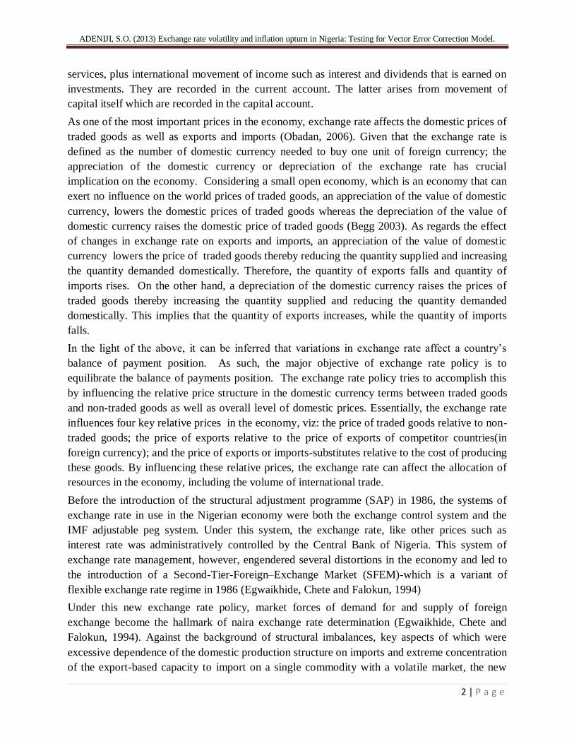
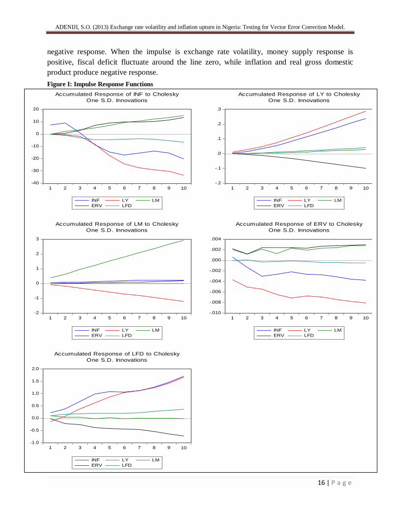
5.6 Impulse Response Function (IRF)

Impulse response function depicts the reaction of a dynamic system to a brief input signal

or some external change, called an impulse. It describes the reaction of the system as a function

of time (or possibly as a function of some other independent variable that parameterizes the

dynamic behavior of the system). It investigates the effect of cholesky one S.D innovation on the

behavior of the time series. Therefore, we present the analysis of accumulated impulse responses

of economic variables as thus:

From the below figure I, the first figure is the impulse of inflation, exchange rate volatility and

money supply response is positive, while fiscal deficit and real gross domestic product produce a


16 | P a g e

negative response. When the impulse is exchange rate volatility, money supply response is

positive, fiscal deficit fluctuate around the line zero, while inflation and real gross domestic

product produce negative response.

Figure I: Impulse Response Functions

5.7 Variance Decomposition

The variance decomposition shows the amount of information each variable contributes to the

other variables in the autoregression. It uncovers how much of the forecast error variance of each

of the variables can be explained by exogenous shocks to the other variables. Given a ten year

forecasting time horizon, variance decomposition of inflation is shown below:

Table 5.7 Variance Decomposition

Variance Decomposition

of INF:

Period S.E. INF LY LM ERV LFD

1 7.485426 100.0000 0.000000 0.000000 0.000000 0.000000

2 8.046867 90.13754 20.15856 7.740434 0.408956 1.297211

3 12.01935 85.71605 17.98375 4.367218 4.534778 4.083577

4 17.24778 71.09199 15.16025 3.203817 7.734290 2.809655

5 20.72107 58.47354 14.98989 3.210966 6.378742 1.946868

6 21.98249 53.03726 13.65373 3.784013 5.743172 1.781824

7 22.30896 51.93179 11.72964 4.011364 5.576500 1.750703

8 22.48324 51.79929 10.60766 4.349669 5.506227 1.737159

9 22.68226 51.38126 7.378803 4.657591 5.677515 1.904833

10 23.66038 51.66509 6.450392 4.738848 6.104518 2.040624

From the above table, the second column gives the standards error (SE) i.e. the forecast error of the variable at different periods, the third column refers to INF, the fourth LY, the fifth LM, the six ERV and the last LFD. Variance decomposition of INF show a self-explained power in the first period as none of other variables could account for its variability. After the first period, variables like LM, ERV and LFD were gradually increasing inflation, while LY were declining. However, in the tenth period, LY, LM, ERV and LFD explain about 6.4 percent, 4.7 percent, 6.1 percent and 2 percent respectively on INF. It can then be deduced that, LY at 6.4 percent produce the highest percent variability in INF in that period despite its declining form.

-40

-30

-20

-10

0

10

20

1 2 3 4 5 6 7 8 9 10

INF LY LM

ERV LFD

Accumulated Response of INF to Cholesky

One S.D. Innovations

-.2

-.1

.0

.1

.2

.3

1 2 3 4 5 6 7 8 9 10

INF LY LM

ERV LFD

Accumulated Response of LY to Cholesky


-2

-1

0

1

2

3

1 2 3 4 5 6 7 8 9 10

INF LY LM

ERV LFD

Accumulated Response of LM to Cholesky


-.010

-.008

-.006

-.004

-.002

.000

.002

.004

1 2 3 4 5 6 7 8 9 10

INF LY LM

ERV LFD

Accumulated Response of ERV to Cholesky


-1.0

-0.5

0.0

0.5

1.0

1.5

2.0

1 2 3 4 5 6 7 8 9 10

INF LY LM

ERV LFD

Accumulated Response of LFD to Cholesky



17 | P a g e

VI Conclusion

This paper empirically analyzes the impact of exchange rate volatility on inflation a

vector error correction model and granger causality approach in Nigeria over a period of 1986 to

2012. Exchange rate volatility was not considered alone but efforts were made to investigate the

impact of other variables such as money supply, real gross domestic product and fiscal deficit.

The result from the vector error correction model shows that exchange rate volatility, money

supply and fiscal deficit positively and significantly related to inflation, while real gross

domestic product gives a negative and insignificant relationship. The granger causality result is

akin to the above result given a uni-directional and bi-directional relationship among the

variables. Hence, the result of this empirical analysis strongly supports various economic

theories. Therefore, the following recommendations are necessary for policy making on inflation

in Nigeria.

Firstly, there is the need to understand the various channels through which exchange rate

transmits to affect inflation in Nigeria. The present situation is that most people are not well

informed about the detrimental effect of exchange rate volatility. A proper study of the causes of

exchange rate variability will help in minimizing its impact on macroeconomic variables.

Secondly, there is the need for the central bank of Nigeria to check the growth of money supply.

This is necessary as a positive relationship exists between the level of money supply and

inflation.

Thirdly, every effort should be channeled it expenditure to the key productive sectors of the

economy such as agriculture and manufacturing this will go a long way in increasing the

production of goods and services which is capable of stabilizing prices and reduce inflation given

their negative relationship.

Lastly, the size of the public sector expenditure needs to be reduced and possibly make a shift

from excessive consumption expenditure to capital expenditure. Doing this will reduce the

burden of fiscal deficit and the rate of inflation


18 | P a g e

REFERENCES

Aydin, B. (2010) ―Exchange Rate Assessment for Sub-Saharan Economies IMF Working Paper

10, pp. 1-62.

Begg, K. (2003). ―Term of trade and Exchange Rate Regimes in developing countries, Journal of

International Economics, 63(1), pp. 31-58.

Blanchard, O. (2000). Macroeconomics (Second ed.). Prentice Hall.

Canetti, Elie, and Joshua Greene (1991). ―Monetary Growth and Exchange Rate Depreciation as

Causes of Inflation in African Countries: An Empirical Analysis‖. IMF Working Paper,

Washington, D.C.: International Monetary Fund.

Egwaikhide, Festus O., Louis N. C. and Gabriel O. F. (1994). ―Exchange Rate Depreciation,

Budget Deficit and Inflation - The Nigerian Experience‖. AERC Research Papers, 26,

Nairobi: African Economic Research Consortium.

Elbadawi, I. A. (1990). ―Inflationary Process, Stabilization and the Role of Public Expenditure in

Uganda.‖ Washington, D.C.: World Bank.

Fisher, I. (1973). ―I discovered the Phillips curve: ‗A statistical relation between unemployment

and price changes‘‖. Journal of Political Economy 81(2), pp. 496–502.

Frankel, J. and Andrew R. (1996). ―A Survey of Empirical Research on Nominal Exchange

Rates.‖ In Gene Grossman and Kenneth Rogoff, eds., Handbook of International

Economics. Amsterdam: North-Holland.

Friedman, M. (1992). ―Money Mischief: Episodes in Monetary History‖. New York: Harcourt

Brace Jovanovich.

Geoff, R. (2006). ―An Assessment of Currency Devaluation in Developing Countries‖. Essays in

International Finance, no. 86. Princeton, N.J.: Princeton University.

Gujarati, D. N. (1995). Basic Econometrics, Third Edition, McGraw Hill International Edition.

Kamin, S. B. and Khan, M. (2003). ―A multi-country comparison of the linkages between

inflation and exchange rate competitiveness‖. International Journal of Finance and

Economics, 8, pp. 167-183.

Khan, G. A. (1989). ―The Output and Inflation Effects of Dollar Depreciation.‖ Federal Reserve

Bank of Kansas City, Research Working Paper 85-05. Kansas City: Federal Reserve

Bank of Kansas City.

Lu, M. and Z. Zhang (2003). ―Exchange Rate Reform and Its Inflationary Consequences: An

Empirical Analysis for China‖. Applied Economics. 35(2), pp. 189-199.

Montiel, P. J, (1989). Macroeconomics in Emerging Markets. Cambridge: Cambridge University

Press.

Obadan, M. I. (2006). ―Overview of exchange rate management in nigeria from 1986 to date‖, in

the ―Dynamics of Exchange Rate in Nigeria‖, Central Bank of Nigeria Bullion, 30 (3),

pp. 17-25.

Odedokun, M. O. (1996). ―Dynamics of Inflation in Sub-Saharan Africa: The Role of Foreign

Inflation; Official and Parallel Market Exchange Rates; and Monetary Growth.‖ Dundee,

Scotland: University of Dundee.


19 | P a g e

Odusola, A. F. and A. E. Akinlo (2005). ―Output, Infl ation, and Exchange Rate in Developing

Countries: An Application to Nigeria‖. The Development Economies XXXIX, pp. 199-

222.

Omotor, D. G. (2008). ―Exchange rate reform and its inflationary consequences: the case of

Nigeria‖. EKONOMSKI PREGLED, 59 (11), pp. 688-716.

Taylor, M. (1995). ―The Economics of Exchange Rates.‖ Journal of Economic Literature, 33(1),

pp. 13–47.

Yoon, G. (2009). ―Are Real Exchange Rates more likely to be Stationary during the fixed

Nominal Exchange Rate Regime?‖ Applied Economic Letters, 16, pp.17-22.

Documents

Munich Personal RePEc Archive - uni- · PDF fileFalokun, 1994). Against the background of structural imbalances, key aspects of which were excessive dependence of the domestic production