MPRAMunich Personal RePEc Archive

Education as a driver of incomeinequality in twentieth-century Africa

Bas Van Leeuwen and Jieli van Leeuwen-Li and Peter

Foldvari

Utrecht University Faculty of Humanities Research Institute forHistory and Culture

20. October 2012

Online at http://mpra.ub.uni-muenchen.de/43574/MPRA Paper No. 43574, posted 5. January 2013 03:09 UTC

Education as a driver of income inequality in twentieth-century Africa

Bas van Leeuwen (Utrecht University) bas.vanleeuwen1@googlemail.com

Jieli van Leeuwen-Li (Utrecht University)

Peter Foldvari (Utrecht University)

In this paper, we address the issue of how education affected income inequality in twentieth-century

Africa. Three channels are identified through which education may affect income inequality. First,

an increase in the average educational level is correlated with an increase in average income, which,

ceteris paribus, reduces inequality. Second, a reduction in educational inequality may, given a

positive correlation between education level and income, reduce income inequality. Thirdly, an

increase in the supply of education may decrease the price of skilled labour thus lowering income

inequality.

We find that in the long-run education does not affect income growth, indicating that in

twentieth-century Africa it was inspiration (i.e., Total Factor Productivity [TFP]) rather than

perspiration (i.e., education and physical capital) that drove economic development. Testing for the

effects of the remaining two channels, we found a significant non-linear relationship between

educational and income inequality suggesting that, contrary to the level of education, these two

channels were important in determining income inequality in Africa. Taking an example from the

end of the twentieth century, if educational equality had been eliminated, then income inequality

would decline by no less than 81%.

I

Education is often considered the driver of economic welfare. It has a direct effect on income by

increasing labour productivity1 and an indirect effect by improving institutional structures by

enhancing democracy2 or reducing corruption,

3 even though this relationship is not necessarily

monotonic.4 Yet remarkably little attention has been paid to the role of education in the much

discussed 'African growth tragedy'. For lack of data, much of the discussion has focussed on what

may be called the 'ultimate sources of growth', i.e., geographical and biological factors5 and

institutional ones such as colonial policy6 rather than on the proximate sources like factor

endowments. Indeed, '[f]actor endowments […] have gone out of focus for a generation of

economic historians more impressed by the importance of institutions and information problems in

shaping economic behaviour'.7

This literature is generally pessimistic about Africa's future, since its geographical and

institutional endowments are unlikely to improve significantly, and the negative consequences of its

colonial past are liable to continue to take a heavy toll for the foreseeable future. Due to their

persistence over time, neither of these factors can account for catastrophic reversals of fortune.8

Based on these studies, it is hard to believe today that during the 1960s African growth potential

outstripped that of Asia. However, it is the fact that geographical and institutional forces are

channelled through shifting factors of production that explains the shifting nature of Africa's

fortunes.9

Especially education has been widely recognised as a factor of production that drives long-

1 For example, Nelson and Phelps, ‘Investment in humans’; Lucas, ‘On the mechanics’; Romer, ‘Endogenous

technological change’. 2 For example, Perotti, ‘Growth, income distribution, and democracy’; Alessina and Perotti, ‘Income distribution,

political instability, and investment’. 3 Mauro, ‘Corruption and growth’.

4 Eicher et al., ‘Education, corruption, and the distribution of income’.

5 See for example, Sachs and Warner, ‘Economic convergence and economic policies’; Gallup et al., ‘Geography and

economic development’. 6 North, Summerhill, and Weingast, ‘Order, disorder, and economic change’. Easterly and Levine, ‘Africa’s growth

tragedy’; Acemoglu et al., ‘Reversal of fortune’; Rodrik, . ‘Institutions rule’. 7 Austin, ‘Resources, techniques, and strategies’, p. 587.

8 Prados de la Escosura and Smits, ‘Decolonization and long-run economic performance’, p. 3.

9 Eicher et al., ‘How do institutions’.

+

run economic fortunes. However, for Africa, on the one hand it is widely recognized that Africa is

deficient in regard to education as well as physical capital10

while, on the other hand Prados de la

Escosura finds that education has been the driving force behind the improvement, admittedly

meagre, in the continent's Human Development Index (HDI) since the 1930s.11

This latter view is

also shared by Rimmer in the case of late colonial Ghana for which he argued that growth was not

limited by lack of skilled labour.12

The focus of this paper is therefore on the effect of education on economic inequality among

African nations since the early 1930s. It is organized as follows. Beginning Section 2 with a

discussion of welfare trends, we distinguish three effects. One of them -- that of education on per

capita income and, ceteris paribus, on income inequality -- will be the subject of Section 3. We find,

however, that the impact of education on income is both insignificant and indirect. Section 4 than

moves on to the other two channels through which education affects income inequality. We find that

if educational inequality decreases, so will income inequality. Likewise, we find that an excess

supply of education lowers its price and hence income inequality as well. We end with a brief

conclusion.

II

For lack of data, the question of how income and education in Africa evolved over the course of the

twentieth century, especially prior to about 1950, cannot be answered with any precision.

Maddison (2007) is virtually our sole source (a few benchmark estimates) of data on per capita

GDP for the first half of the century and our chief source for the second half.13

For the years after

ca. we draw on the Conference Board's Total Economy Database (2012).14

There are three ways to remedy the inadequacy of the data on changes in regional per capita

10

E.g., Cohen and Soto, ‘Why are some countries so poor?’; Frankema, ‘The origins of formal education’. 11

Prados de la Escosura, ‘Human development in Africa’. 12

Rimmer, Staying poor. 13

Maddison, Contours of the world economy. 14

Conference Board, Total Economy Database (TED), Output, Labor and Labor Productivity Country Details, 1950-

2011.

income in Africa prior to 1950 (the regions being those defined by the United Nations: North, West,

Central, East, and Southern)15

. First, some data exist for a few countries. Second, we can draw on

real-wage data in the work of Frankema and Van Waijenburg to proxy per capita income (2011)16

provided that there is no significant change in the share of wage income in total income and in the

number of days worked.17

Third, we can use Prados de la Escosura's preliminary estimates of GDP

per capita, which he made by running a regression of GDP per capita on the income terms of trade

per head, a time trend, and several dummy variables capturing colonizer effects, regional effects,

and a dummy for countries with access to the sea.18

Unfortunately, however, since we cannot

assume that the relation between terms of trade and per capita GDP remains unchanged, we risk

underestimating the level of the latter during the first half of the century. Thus while each

estimation method if used in isolation has significant drawbacks, they are quite useful when used in

combination, functioning as they do as cross-checks.

For North Africa, we obtain data from GDP estimates by Amin (1966), covering benchmark

years between 1880 and 1955 for Algeria, between 1910 and 1955 for Tunisia, and between 1920

and 1955 for Morocco.19

All of these data are connected to the 1950 benchmark expressed in 1990

GK dollars. For Egypt, our data come from Yousef (2002).20

We assume that the population-

weighted average of per capita GDP of these countries reflects the trend in North Africa for the

period before 1950 (see Table 1). However, since Yousef’s data, especially for the years prior to

1900, indicate higher growth rates than do those of Hansen and Marzouk (1965) and of Hansen

(1979, 1991)21

our estimates for 1890 are slightly lower than they would have been had we used

Hansen's data. One way to cross-check this result is to compare it with those of Prados de la

15

North Africa: Algeria, Egypt, Libya, Morocco, Sudan, Tunisia; West Africa: Benin, Burkina Faso, Ivory Coast,

Gambia, Ghana, Guinea, Liberia, Mali, Mauritania, Niger, Nigeria, Senegal, Sierra Leone, Togo; East Africa:

Burundi, Ethiopia, Kenya, Madagascar, Malawi, Mauritius, Mozambique, Rwanda, Seychelles, Somalia, Tanzania,

Uganda, Zambia, Zimbabwe; Central Africa: Angola, Cameroon, Central African Republic, Chad, Congo

(Brazzaville), Congo (Kinshasa), Gabon; Southern Africa: Botswana, Namibia, South Africa, Swaziland. 16

Frankema and Van Waijenbrug, ‘African real wages’. 17

Angelis, ‘GDP per capita or real wages?’. 18

Prados de la Escosura, ‘Human development in Africa’. 19

Amin, L’économie du Maghreb, pp. 104-5. 20

Yousef, ‘Egypt’s growth performance’. 21

Hansen and Marzouk, Development and economic policy; Hansen, ‘Income and consumption in Egypt’; Hansen,

The political economy of poverty.

Escosura (2011), who finds GDP per capita in North Africa in 1890 to be 802 GK dollars, versus

our 559.22

The main reason for this difference is Egypt. Unfortunately, it is difficult to substantiate

which series to believe. The series from Yousef (2002), on which our series is based, is in line with

the real wage series for Egypt,23

while the Hansen (1979, 1991) series decline less back to 1880.

For West and East Africa, GDP data are scantier. Szereszewski's 1891-1911 and 1966 Ghana

data24

are the best that we have for West Africa. However, he presumes that change occurs only in

the 'modern' sector; since the indigenous sector is far larger, his results indicate that economic

development was more limited than, in fact, it was. Yet, according to real wage series provided by

Frankema and Van Waijenburg (2011),25

between 1890 and 1950 the indigenous economy generated

a significant increase in per capita income. Using their real-wage data, we find that in 1890 Ghana's

GDP was roughly 760 GK dollars, compared to ca. 516 from Prados de la Escosura.26

This

discrepancy suggests that a trade-based approach may lead to an underestimation of GDP for West

Africa in general. For East Africa, data are even scarcer: Deane (1946) estimated the national

income of Northern Rhodesia (i.e., Zambia) at 7.63 mln GDP in 1938 or 418 1990 GK dollars.

Fortunately, we also have the numbers for real wages (Frankema and van Waaijenburg 2011), which

show that (assuming that they move in line with per capita income) average GDP per capita in 1910

was about 484 GK dollars.27

For the Southern region (i.e., South Africa, Swaziland, Lesotho,

Namibia, and Botswana), we converted data from Krogh and Willers (1962)28

into constant prices

and linked these per capita GDP series to the 1950 benchmark average of these five countries.

The resulting estimates of GDP per capita in Africa are reported in Table 1. The average

African per capita GDP increases from 683 GK dollars in 1900 to 2,023 GK dollars around 2010: .

slightly higher than the estimate of Smits (2006), 524 GK dollars, for sub-Saharan Africa in 1913.29

Corrected for North Africa from Table 1, this results in an overall African GDP per capita from

22

Prados de la Escosura, ‘Human development in Africa’. 23

Williamson, ‘Real wages and factor prices’. 24

Szereszewski, Structural changes in the economy of Ghana, pp. 74, 92-3, 126-49. 25

Frankema and Van Waijenbrug, ‘African real wages’. 26

Prados de la Escosura, ‘Human development in Africa’. 27

Frankema and Van Waijenbrug, ‘African real wages’. 28

Krogh and Willers, ‘The preparation of national accounting estimates’, Table 1. 29

Smits, ‘Economic growth and structural change’.

ª

Smits of about 610 GK dollars. Likewise, Prados de La Escosura30

estimated average per capita

GDP for Africa around 1913 at 772 GK dollars. The three methods thus generate similar results,

Table 1. Per capita GDP in Africa by sub-region, ca. 1890-2010

North

Africa

West

Africa

Central

Africa

East

Africa

Southern

Africa Total

Africa

1890 559 752

1900 714 863 508 683

1910 832 586 484 641

1920 960 867 771 871 836

1930 1,059 1,230 600 1,329 976

1940 1,075 718 728 1,909 889

1950 1,085 757 729 800 2,425 968

1960 1,279 871 909 953 2,919 1,151

1970 1,648 1,098 1,036 1,178 3,904 1,459

1980 2,285 1,217 888 1,155 4,257 1,657

1990 2,354 1,041 812 1,061 3,764 1,549

2000 2,712 1,024 577 1,031 3,886 1,575

2010 3,590 1,436 749 1,245 4,972 2,023

with Southern Africa growing significantly faster than the other regions, with the exception of

North Africa since the 1970s, which obviously profited from its oil reserves. Per capita income

stagnated in all of the other regions except Central Africa, where it declined. To explain this income

divergence among countries, which, as we shall see in Section 4 also occurred within countries, we

turn our attention to the factors that affected this distribution of income, and most importantly,

education.

As for education, the earliest estimates are from Benavot and Riddle, who report primary

enrolment ratios (i.e., the total number of students divided by the relevant age class) for the period

1870-1940.31

The most interesting finding is that the primary-school enrolment rates in sub-Saharan

and North Africa are not significantly different. However, this result is liable to reflect a sample-

selection bias, since national enrolment rates tend to be directly correlated with statistical coverage.

In another study, Morrisson and Murtin (2009) estimated average years of education for every tenth

30

Prados de la Escosura, ‘Human development in Africa’, Table D-4. ). 31

Benavot and Riddle, ‘The expansion of primary education’.

year for a set of 23 African countries between 1870 and 2010.32

For the period after 1960 they based

their data largely on Cohen and Soto (2007),33

while for the pre-1960 period they assumed that

enrolment declines steadily back to zero at the start of the nineteenth century. Finally, the most

comprehensive dataset in terms of the number of countries covered is that of Barro and Lee (2010),

who provide data on average years of education for most of the countries under study for every fifth

year since 1950.34

Unfortunately, these datasets do not contain annual data nor do they cover a broad sway

swathe of countries and/or time periods. The only dataset that contains annual estimates (Nehru et

al. 1995)35

covers only the period 1960-1987 and is furthermore based on a perpetual-inventory

method (PIM), generally considered less reliable than estimates based on census data. Our first

order of business in this paper, therefore, was to establish a new set of annual estimates of average

years of education for most African countries; the method we used -- described in Van Leeuwen and

Foldvari (2012)36

-- relies on census data for benchmark years, derived mostly from Cohen and

Soto (2007).37

Estimates for the intervening years are calculated by means of the PIM-methodology

as proposed in Barro and Lee (2001).38

Since this method leads to an overestimation when

calculating backward and an underestimation when calculating forward, we use a weighted average

of the two sets of figures.39

For the period before the first census, we use a perpetual-inventory

32

Morrisson and Murtin, ‘The century of education’. 33

Cohen and Soto, ‘Growth and human capital’. 34

Barro and Lee, ‘A new dataset on educational attainment’. 35

Nehru et al., ‘A new database on human capital stock’. 36

Van Leeuwen and Foldvari, ‘Capital accumulation and growth’. 37

Cohen and Soto, ‘Growth and human capital’. 38

Barro and Lee, ‘International comparisons of educational attainment’. 39

In the most recent version of their dataset Barro and Lee, ‘A new dataset on educational attainment’ use additional

information on mortality to correct for this bias, but this requires additional data usually unavailable for historical

research, and for developing regions. For this reason we prefer the simpler but feasible method in Van Leeuwen and

Foldvari, ‘Capital accumulation and growth’.

ª

Table 2. Population weighted average years of education in Africa, ca. 1890-2010

Nehru et

al.

(1995)

Baier, et.

al. (2006)

Cohen

and Soto

(2007)

Morrisson

and

Murtin

(2009)

Barro

and Lee

(2010) This text

1890 0.2

1900 0.2

1910 0.2 **0.3

1920 0.3 0.3

1930 0.4 0.5

1940 0.5 0.6

1950 1.5 0.7 0.8 0.9

1960 0.9 2.1 1.2 1.1 1.0 1.2

1970 1.3 2.8 1.5 1.5 1.4 1.7

1980 1.9 3.3 2.0 2.2 2.1 2.3

1990 *2.5 4.2 2.9 3.2 3.0 3.4

2000 4.8 3.7 4.0 3.6 4.3

2010 4.1 4.5 4.1 4.9

*1987, **1915

method, which corrects for age-specific mortality. The enrolment data are obtained from UNESCO

through the intermediary of the Education Policy and Data Center (accessed 2011), Mitchell (1999),

and for earlier periods from Frankema (2012) and the House of Commons Parliamentary Papers

(various issues).40

The population data were obtained from Maddison (2007), the United States

Census Bureau, International Programs (accessed 2011), and the House of Commons Parliamentary

Papers (various issues).41

The results are reported in Table 2 together with some competing estimates. Our estimates

are virtually identical to those of Cohen and Soto (2007) and Morrisson and Murtin (2009),42

there

being few differences for the post-1960 period. Two differences between our series and those of

Morrisson and Murtin are worth noting: our dataset includes about twice as many countries, and we

do not find the enrolment ratio going linearly back to zero at the start of the nineteenth century.

To test the relative reliability of our series, we regressed each of two alternative estimates of

40

Education Policy and Data Center (accessed 2011); Mitchell, International historical statistics; Frankema, ‘The

origins of formal education’; House of Commons, ‘Statistical Tables’. 41

Maddison, Contours of the world economy; United States Census Bureau, ‘International Programs’; House of

Commons, ‘Statistical Tables’. 42

Cohen and Soto, ‘Growth and human capital’; Morrisson and Murtin, ‘The century of education’.

ª

the same latent variable on the other.43

Since the measurement error of the dependent variable will

not affect the OLS estimate of the slope coefficient, the resulting coefficient may be interpreted as

the error-to-signal ratio in the explanatory variable. The results are reported in Table 3. Our

Table 3. Reliability ratio average years of education

Barro and Lee

(2010)

(1950-2010)

Baier et al. (2006)

(1917-2000)

Cohen and Soto

(2007)

(1960-2010)

Morrisson and

Murtin (2009)

(1870-1950)

Morrison and

Murtin (2009)

(1950-2010)

estimated error-

to-signal variance

ratio, compared

to own estimates

36.5% 297% 5.2% 13.3% 11.7%

the estimated

error-to-signal

variance ratio of

own estimates

compared with

other estimates.

11.1% 13.1% 0% 11.9% 8.3%

Note: measurement error variance relative to signal variance, a lower number means less noisy estimates

estimates outperform those of Barro and Lee (2010) and Baier et al. (2006) significantly44

but those

of Cohen and Soto and of Morrisson and Murtin only slightly, since they are based on similar

data.45

When we use these data to look at the long-run pattern of education in Africa by sub-region,

we find that Southern Africa did especially well in terms of years of education throughout most of

the twentieth century (Table 4 and Map 1), only the North eventually catching up, after the 1970s.

The validity of these results, however, has been confirmed by Crayen and Baten (2007), who, using

age-heaping methodology, found a remarkably high degree of age heaping (hence a low numeracy)

in North Africa in 1890 followed by a gradual improvement. One might argue that a Muslim

presence might explain the fact that until the 1970s North Africa performed poorly, in terms

43

Krueger and Lindahl, ‘Education for growth’. 44

Baier et al., ‘How important are capital and total factor productivity’; Barro and Lee, ‘A new dataset on educational

attainment’. 45

Cohen and Soto, ‘Growth and human capital’; Morrisson and Murtin, ‘The century of education’.

ª

Table 4. Average years of education in Africa by sub-region, ca. 1890-2010

North

Africa

West

Africa

Central

Africa

East

Africa

Southern

Africa Total

Africa

1890 0.1

1900 0.1

1915 0.2 0.1 0.2 1.8 0.3

1920 0.3 0.1 0.3 2.0 0.3

1930 0.4 0.2 0.2 0.5 2.4 0.5

1940 0.5 0.3 0.3 0.8 2.9 0.6

1950 0.7 0.4 0.5 1.0 3.5 0.9

1960 0.9 0.8 0.8 1.5 4.2 1.2

1970 1.4 1.2 1.2 1.9 4.7 1.7

1980 2.4 1.5 2.0 2.4 5.1 2.3

1990 3.9 2.5 3.1 3.3 5.7 3.4

2000 5.2 3.4 3.6 4.0 7.2 4.3

2010 6.1 3.9 4.0 4.5 8.5 4.9

Map 1. Average years of education in Africa, 2010

(6.32715,10.4053](4.54657,6.32715](3.34713,4.54657][1.42827,3.34713]No data

of both average years of education and numeracy, but Crayen and Baten (2007) cast doubt on this

explanation, observing that nearby Christian and Hindu populations had not appreciably higher

ª

levels of numeracy.46

In addition, both numeracy and years of education varied considerably

throughout the region, Algeria and Tunisia having the highest rates on both counts. Egypt had the

lowest numeracy rate, but this may be because Sudan and Libya were not included in the numeracy

dataset However, in the average years of education dataset they rated below Egypt.

These findings hint at a statistical relationship between educational attainment and per capita

income. After all, per capita income as well as the level of education was clearly higher in Southern

African than in the remainder. Likewise, the economic expansion in North Africa coinciding as it

did with the improvements on the education front in the 1970s. Still, a simple co-movement of

education and per capita income is not evidence of a structural/causal relationship, and any two-

variable statistical approach we might use to find such a structural relationship would suffer from a

bias due to the omission of the remaining factor of production: physical capital -- to which we will

now, therefore, briefly turn our attention.

We draw on five datasets: those of Baier, Dwyer and Tamura (2006), Miketa (2004),

Easterly and Levine (2002), Nehru and Dhareshwar (1993), and the extended Penn World Tables

(Marquetti and Foley 2011).47

Given the differences in methodology, it is impossible to estimate the

reliability ratio for the data.48

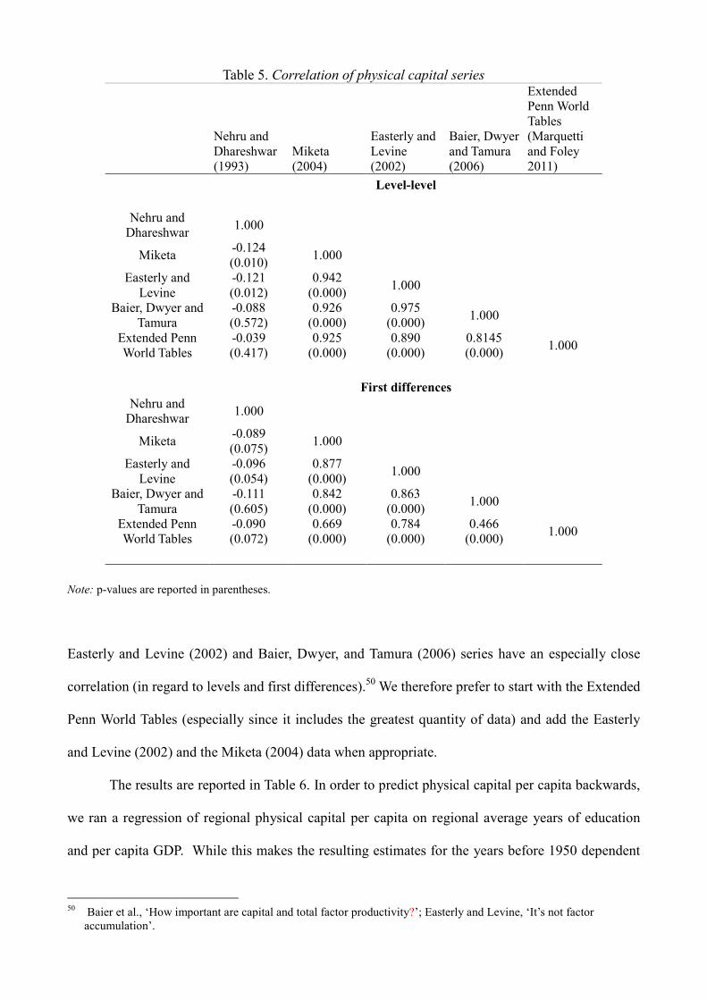
The linear correlation coefficients among the different series, which

are reported in Table 5, may shed some information on their reliability though. It seems clear that

the Nehru series constitute the major outlier, being negatively correlated with the other series, in

regard to levels and first differences.49

The other series are largely comparable, even though the

46

Crayen and Baten, ‘Global trends in numeracy’. 47

Baier et al., ‘How important are capital and total factor productivity’; Miketa, ‘Technical description on the growth

study datasets’; Easterly and Levine, ‘It’s not factor accumulation’; Nehru and Dhareshwar, ‘A new database on

physical capital stock’; Marquetti and Foley, ‘Extended Penn World Tables’. 48

The reason is that the OLS-based estimate of the reliability ratio requires that the observed series be unbiased

estimates of the underlying, latent variable. Since the five capital-stock estimates mentioned in the text exhibit very

different trends, at least some of them must be biased. Consequently, the OLS estimates of the reliability ratio would

also have a component resulting from the bias, and this cannot be isolated. 49

Nehru and Dhareshwar, ‘A new database on physical capital stock’.

B

Table 5. Correlation of physical capital series

Nehru and

Dhareshwar

(1993)

Miketa

(2004)

Easterly and

Levine

(2002)

Baier, Dwyer

and Tamura

(2006)

Extended

Penn World

Tables

(Marquetti

and Foley

2011)

Level-level

Nehru and

Dhareshwar 1.000

Miketa -0.124

(0.010) 1.000

Easterly and

Levine

-0.121

(0.012)

0.942

(0.000) 1.000

Baier, Dwyer and

Tamura

-0.088

(0.572)

0.926

(0.000)

0.975

(0.000) 1.000

Extended Penn

World Tables

-0.039

(0.417)

0.925

(0.000)

0.890

(0.000)

0.8145

(0.000) 1.000

First differences

Nehru and

Dhareshwar 1.000

Miketa -0.089

(0.075) 1.000

Easterly and

Levine

-0.096

(0.054)

0.877

(0.000) 1.000

Baier, Dwyer and

Tamura

-0.111

(0.605)

0.842

(0.000)

0.863

(0.000) 1.000

Extended Penn

World Tables

-0.090

(0.072)

0.669

(0.000)

0.784

(0.000)

0.466

(0.000) 1.000

Note: p-values are reported in parentheses.

Easterly and Levine (2002) and Baier, Dwyer, and Tamura (2006) series have an especially close

correlation (in regard to levels and first differences).50

We therefore prefer to start with the Extended

Penn World Tables (especially since it includes the greatest quantity of data) and add the Easterly

and Levine (2002) and the Miketa (2004) data when appropriate.

The results are reported in Table 6. In order to predict physical capital per capita backwards,

we ran a regression of regional physical capital per capita on regional average years of education

and per capita GDP. While this makes the resulting estimates for the years before 1950 dependent

50

Baier et al., ‘How important are capital and total factor productivity?’; Easterly and Levine, ‘It’s not factor

accumulation’.

on GDP and education we have no reason to omit them, since they will not be used in the

regressions presented in the following sections. We find that the level of physical capital was

Table 6. Per capita physical capital in Africa by sub-region, ca. 1920-2010

North

Africa

West

Africa

Central

Africa

East

Africa

Southern

Africa Total

Africa

1920 753 617

1930 1,032 904 647 803 890

1940 1,287 745 1,254 798 1,434 1,015

1950 1,538 796 1,077 932 2,404 1,155

1960 1,679 988 921 1,056 3,788 1,403

1970 2,094 1,116 939 1,256 5,376 1,691

1980 4,102 1,403 1,139 1,697 7,336 2,560

1990 4,527 1,015 1,058 1,603 6,059 2,410

2000 3,875 756 844 1,630 5,625 2,062

2010 4,881 944 819 1,764 7,250 2,439

Map 2. Physical capital/GDP ratio in Africa , 1960

(1.54942,4.78272](.95135,1.54942](.607721,.95135][.070858,.607721]No data

especially high in Southern Africa, whereas in North Africa it soared only after the 1970s (see also

Map 2). West and Central Africa were at the back of the pack. It is thus evident not only that

B

educational level, but also physical capital is correlated with per capita GDP. However, this does not

tell us anything yet about causation (i.e. whether it is education, conditional upon the presence of

physical capital, that affects per capita income or vice versa). This is the topic of the following

Section.

III

As we have just seen, a rise in the average level of education is correlated with a rise in the level of

per capita income and thus a decline in the overall level of inequality.51

Those who argue that

growth in Southeast Asia has been driven mostly by factors of perspiration (i.e., the factors of

production) rather than those of inspiration (i.e., TFP)52

might very well argue that this correlation

also represents causation (i.e. education affecting per capita GDP instead of the reverse) in regard to

Africa.

However, an analysis of the role of education in economic growth requires an understanding

of its dual role: as a human-capital channel and as the cornerstone of national institutional structures

that address basic quality-of-life issues, including health care. Whereas the second role directly

relates education to institutions and social variables, the first role is more controversial since it

generally refers to human capital rather than education. Yet, since human capital is a latent variable

there is no consensus on how this channel functions; the most popular approach is simply to use

education as a proxy thereof. A second possible way is to use the so-called Mincerian human

capital53

the idea being that the per capita stock of human capital can be estimated from average

years of education (St) and the rate of private returns to education (rt) as follows:

ln t t th r S= (1)

where the change of the rate of return on education over time is often assumed to be a function of

51

To understand why, see ‘A simple way to calculate the Gini coefficient’ in which Milanovic derives the relation

between the Gini coefficient and the Coefficient of Variation (CV), which is the standard deviation divided by the

mean. If the CV increases by 1 unit the Gini coefficient will increase by 1

3unit.

52 Krugman, ‘The myth of Asia’s miracle’.

53 For example, Hall and Jones, ‘Why do some countries produce so much more output per worker than others?’;

Pritchett, ‘Where has all the education gone?’.

B

the average years of education.

We have already critiqued the various approaches in other papers;54

so this time, our purpose

is, instead of analyzing how human capital affects per capita income, to analyze the role of

education in income inequality. Not only is education one of the most important way to empirically

capture human capital, but it is also the variable that governments can most easily manipulate and,

as such, function as an important policy objective. Hence, seeing how education affects income

inequality is very useful from a policy perspective.

A simple way to determine both the short- and the long-run relationships between per capita

income and education is to estimate an error-correction representation of the production function of

per capita GDP, with physical capital and education as explanatory variables. The direction of

causality is irrelevant, since we are looking for a long-run equilibrium relationship (cointegration).

The unit-root tests (see Table A1) suggest that all variables are integrated of order one, so the

theoretical possibility of cointegration does exists. The error-correction specification is as follows:

0 1 2 3 1 4 1 5 1ln ln ln lnit it it it it it i t ity k S y k S uβ β β β β β η λ− − −∆ = + ∆ + ∆ + + + + + + (2)

where lny, lnk, and S denote the per capita GDP, per capita physical capital stock, and the average

years of education. The immediate effects are reflected in the coefficients β1 and β2, while the long-

run coefficients (cointegrating vector elements) and the adjustment coefficient can be estimated

from the coefficients β3-β5. For comparison we also report the coefficients from a level-on-level

specification (static panel), but the presence of a high degree of first-order autocorrelation in the

residuals is a clear sign of a spurious regression.55

While the level-on-level specification seems to suggest that the relationship between

education and per capita income is positive, once we rewrite the specification into an error-

correction model (ECM), it changes to negative, indicating that in the long run an increase in

54

Van Leeuwen and Foldvari, ‘Capital accumulation and growth in Hungary’; Van Leeuwen and Foldvari, ‘Capital

accumulation and growth in Central Europe’. 55

The ECM representation is basically a dynamic panel model, but as T is large, we do no need to worry about the

finite sample bias in fixed-effect dynamic panel models.

B

Table 7. Static and dynamic panel analysis of income on physical capital and education

ln ity ln ity∆

constant 4.257

(9.47)

0.167

(4.89)

ln itk∆ - 0.196

(9.06)

itS∆ - -0.045

(-1.95)

1ln ity − - -0.025

(-3.94)

1ln itk − - 0.004

(1.17)

1itS − - -0.005

(-2.15)

ln itk 0.354

(7.15)

-

itS 0.092

(1.69)

-

R2

0.921 0.164

N 2311 2265 Note: years and country dummies included but not reported.

educational level is correlated with a decrease in per capita income. More specifically, the long-run

effect, -0.005/0.025=-0.2, is economically significant: one additional year of education is correlated

with a 20 per cent decrease in per capita income in the long run.

Moreover, this specification provides no indication of a long-run relationship between

physical capital and per capita GDP. While there is a short-run positive effect, the absence of a

significant coefficient in the cointegrating vector suggests that investments do not cause any

improvement in the factors of production or productivity -- a finding that extends to the second half

of the twentieth century confirming Austin's conclusion that in the long run Africa's production

function consists of a single factor: labour.56

While we are not the first to arrive at these results (see

also Pritchett 2001),57

their counterintuitive nature compels us to cross-check them by means of a

panel VAR analysis.

While this is not yet a standard methodology, it has three advantages over estimating panel

regressions for each of the variables individually. First, it is likely that there is a simultaneous

56

Austin, Labour, land and capital in Ghana, p. 73. 57

Pritchett, ‘Where has all the education gone?’.

relationship between capital stock and per capita income, which would require instrumentation, and

it is very difficult to find adequate time-varying instruments for African countries. Second, since

this analysis involves estimating the impulse-response functions (IRFs), it is more efficient than

other methodologies, permitting us to combine our estimates of the short- and long-run effects.

Third, it obviates the need to specify a system of structural equations, which would be based on

various assumptions requiring verification.

We specify the following PVAR model as follows:

1=

= + + +∑p

j

it i j i,t-j t itY δ Θ Y η u (3)

where ( )ln , ln , ′= it it ity k Sit

Y , iδ and t

η are the country and the time-specific effects, and tu denotes

the vector of the residuals estimated from the PVAR. The country-specific effects are captured by

country dummies, the time-specific effects by a quadratic time trend.

The residuals are likely to be correlated on account of the simultaneous relationship among

the endogenous variables. The primitive form of the above VAR system can be written as:

1=

= + + +∑p

j

it i j i,t-j t itAY α β Y λ ε (4)

where matrix A denotes a matrix of coefficients describing the simultaneous relationship among the

endogenous variables, iα and t

λ are the country- and the time-specific effects, and tε denotes the

vector of equation-specific shocks.

The VAR coefficients will therefore not be equal to the coefficients from the primitive form,

unless there is no simultaneity among the dependent variables (i.e., matrix A is a unit matrix):

1 1 1 1

1

− − − −

=

= + + +∑p

j

it i j i,t-j t itY A α A β Y A λ A ε (5)

As a result, the residuals as estimated from the VAR cannot be used to obtain IRFs without

identifying the matrix A (Structural VAR).

As for the order of the VAR system, we used the Akaike Information Criterion, which

preferred a VAR(9) specification when the quadratic trend was included and a VAR(11) when it was

B

not. At these lag lengths the VAR system fulfilled the stability criterion, which is the fundamental

requirement for obtaining meaningful IRFs. The residual autocorrelation remained insignificant at

one per cent, it was not possible to completely eliminate serial correlation. We tested for

cointegration with the Johansen test, but we found that the matrix П in the following VEC

representation :

1

1

−

=

= + + + +∑p

j

it i j i,t- j i,t-1 t it∆Y δ Γ ∆Y ΠY η u (6)

was of full rank, meaning that the variables are found stationary and cannot by definition be

cointegrated, and allowing us to move for the IRF and the identification of matrix A. The residual

correlation reveals that lny seems to be in a simultaneous relationship with physical-capital stock

and average years of education (Table A2 in the appendix), which is also what we observed in

Section 2. Our identification strategy is based on the dual observation (derived from a Granger

causality test) that a shock in per capita income may affect physical capital and that a shock in

average years of education may affect the log of per capita GDP, but not vice versa.

Figure 1. IRFs and cumulative IRFs from the PVAR

.00

.02

.04

.06

.08

2 4 6 8 10 12 14 16 18 20

Response of LNY

.00

.02

.04

.06

.08

2 4 6 8 10 12 14 16 18 20

Response of LNK

-.02

.00

.02

.04

.06

.08

2 4 6 8 10 12 14 16 18 20

Response of EDUC

Response to One S.D. Innovations in LNY ± 2 S.E.

0.0

0.2

0.4

0.6

0.8

1.0

1.2

2 4 6 8 10 12 14 16 18 20

Accumulated Response of LNY

0.0

0.2

0.4

0.6

0.8

1.0

2 4 6 8 10 12 14 16 18 20

Accumulated Response of LNK

-.2

.0

.2

.4

.6

2 4 6 8 10 12 14 16 18 20

Accumulated Response of EDUC

Accumulated Response to One S.D. Innovations in LNY ± 2 S.E.

B

-.01

.00

.01

.02

.03

2 4 6 8 10 12 14 16 18 20

Response of LNY

.00

.02

.04

.06

.08

.10

.12

2 4 6 8 10 12 14 16 18 20

Response of LNK

-.02

-.01

.00

.01

.02

.03

2 4 6 8 10 12 14 16 18 20

Response of EDUC

Response to One S.D. Innovations in LNK ± 2 S.E.

.0

.1

.2

.3

.4

.5

2 4 6 8 10 12 14 16 18 20

Accumulated Response of LNY

0.0

0.5

1.0

1.5

2.0

2 4 6 8 10 12 14 16 18 20

Accumulated Response of LNK

-.2

-.1

.0

.1

.2

.3

2 4 6 8 10 12 14 16 18 20

Accumulated Response of EDUC

Accumulated Response to One S.D. Innovations in LNK ± 2 S.E.

-.015

-.010

-.005

.000

.005

.010

.015

2 4 6 8 10 12 14 16 18 20

Response of LNY

-.02

-.01

.00

.01

.02

.03

2 4 6 8 10 12 14 16 18 20

Response of LNK

.04

.06

.08

.10

.12

2 4 6 8 10 12 14 16 18 20

Response of EDUC

Response to One S.D. Innovations in EDUC ± 2 S.E.

-.15

-.10

-.05

.00

.05

.10

.15

2 4 6 8 10 12 14 16 18 20

Accumulated Response of LNY

-.2

-.1

.0

.1

.2

.3

2 4 6 8 10 12 14 16 18 20

Accumulated Response of LNK

0.0

0.5

1.0

1.5

2.0

2 4 6 8 10 12 14 16 18 20

Accumulated Response of EDUC

Accumulated Response to One S.D. Innovations in EDUC ± 2 S.E.

The IRFs not only confirm what we already learned from the ECM but also provide an

insight into how education affects both per capita income and capital accumulation. It comes as no

surprise that per capita income has a positive effect on education; since the share of

savings/investments increases in tandem with income, for those of modest means the safest and

most profitable investment is in education. Indeed, several studies have confirmed that the private

rate of returns in Africa is positive.58

On the other hand, it seems that education does not affect per

capita GDP in either the short or the long run, which means that there are virtually no social returns

on education: a finding in line with that of Acemoglu and Angrist (2001) for the United States prior

58

See, for example, Psacharopoulos and Patrinos, ‘Returns to investment in education’

to the 1980s.59

That private returns can be positive while social ones are insignificant or even negative is

counterintuitive, but Pritchett (2001) has found an explanation: a structural mismatch between an

inefficient educational system and the labour market.60

Since positive private returns may exist

simply because of the division of labour, the phenomenon is a cross-sectional/cross-individual one,

an employee's earnings being a function of his or her skills and/or position, which are in turn a

function of educational level; the marginal product of education has to be positive for it to yield any

social returns. Educational level is positively correlated with private returns, but for it to be

Fig. 2 Index of real wages in Africa (1990=100)

Source: Mitchell, ‘International historical statistics’.

correlated with per capita income there has to be a productivity increase at both the individual level

(reflected in a real-wages increase) and the economy-wide one (through spillover effects). We find

no evidence that this has occurred; until the 1980s real wages were outpaced by per capita GDP,

and, worse yet, education's relationship to it was not just flat but negative.

The effects of education may work via other factors of production as well; for instance, it

59

Acemoglu and Angrist, ‘How large are human-capital externalities?’. 60

Pritchett, ‘Where has all the education gone?’.

⢠џ

may be positively correlated with an individual's savings rate, and hence with physical-capital

accumulation. According to the IRFs, however, this is not the case in Africa: even though we obtain

a positive hump in the IRF for capital stock as a response to a shock in education, the magnitude is

insignificant.

Since we also found that a shock in physical capital has only a short-run effect on per capita

GDP growth, it follows that the changes in per capita GDP that occurred toward the end of the

twentieth century were not due to perspiration (i.e. education and physical capital) but rather to

inspiration factors (i.e. TFP). The coefficients of the year dummies from the ECM specification

Fig. 3. TFP as estimated from the ECM specification in Table 7.

(Table 7) can be interpreted as the trend of the growth of general productivity, or TFP (Figure 3).

We also added information on TFP growth back to the 1920s based on a growth-accounting analysis

in which we used the coefficients of education and physical capital from the ECM specification and

the growth of African GDP, physical capital, and education up to 1950 (see the dashed line in Figure

3). We find a set of two trends, in line with the history of twentieth-century Africa: an virtual

absence of improvement until the 1980s and a period of significant improvement afterwards.

That there was no significant TFP growth until the 1980s is in line with the observation of

Hopkins (1973) that in West Africa technology was only of a labour-saving character in the

B

agricultural sector.61

However, Austin shows that this was not the case in manufacturing,62

partly on

account of trypanosomiasis (a parasitic disease, commonly known as sleeping sickness, transmitted

by the tsetse fly) which prevented the large-scale use of animal power.63

Lovejoy shows that in the

mining sector, as well, the lack of know-how prevented the introduction of many labour-saving

technologies:64

an indication that when educational level rises so does TFP.65

We therefore test

Table 8. Relationship between the estimated TFP and education

TFP ∆TFP

constant -0.017

(-3.80)

-0.011

(-2.40)

1itS − 0.006

(3.95)

0.004

(2.66)

TFPt-1 - -0.626

(-5.01)

itS∆ - -0.0097

(-0.44)

R2

0.205 0.312

DW 1.24 2.05 Note: N=57, period: 1951-1998

for the existence of such a relationship, by means of both a level-on-level and an ECM specification

(Table 8) and find that education had a positive impact on TFP, although precisely through what

channels remains to be determined.

We can say, however, that there are two possibilities which both increase TFP growth:

education may improve the technical efficiency of the factors of production (that is, reverse the

trend of diminishing returns to physical capital); and it may improve general productivity (that is,

increase the maximum possible output per worker). Whereas general productivity determines the

production frontier (the maximum possible output per person under optimum circumstances),

technical efficiency determines just how far a country has to go to reach that frontier. We therefore

61

Hopkins, An economic history of West Africa. 62

Austin, ‘Resources, techniques, and strategies’. 63

Austin and Headrick, ‘The role of technology in the African past’, pp. 170-1. 64

Lovejoy, Salt of the desert sun, pp. 112-14. 65

On the other hand, In Staying Poor Rimmer argues that Ghanaian growth during the colonial period was not

obstructed by a lack of educated workers, since they existed in sufficient numbers to keep the cocoa sector

operating.

銰Ѡ

divide TFP growth into a general-productivity and a technical-efficiency index.66

Technical

efficiency is proportional to the elasticity at which factors of production are transformed into

income (or final output). If we assume that this is the same for all geographical units (i), we can

arrive at the standard relative-growth version of the Cobb-Douglas production function:

it t it it

it t it it

y A k Sˆˆy A k S

= +α +β&& &&

(7)

, where t

t

A

A

&

is TFP growth and α̂ and β̂ denote the coefficients in case of no technical

inefficiencies.67

If we allow for technical inefficiency -- that is, if we assume that the coefficients of

the production factors may vary across countries, we arrive at the following form:

( ) ( )it t it it t it it it iti i i i

it t it it t it it it it

y k S k S k Sˆ ˆˆ ˆy k S k S k S

θ θ= +α +β = +α +β + α −α + β −βθ θ

& & && & & & &&

(8)

Where θ is a time-variant common productivity factor (similar to A in the standard-growth

accounting in equation (7) but free of the effect of technical-efficiency differences, and αi

and βi

are

the province-specific coefficients. By combining equations (7) and (8) we can show the

relationships among TFP growth, general-technology growth, and technical efficiency of human -

and physical capital as follows:

( ) ( )t t it iti i

t t it it

A k SˆˆA k S

θ= + α −α + β −βθ

&& & &

(9)

In other words, the traditionally estimated TFP growth consists of the growth of general

productivity (i.e., the outward movement of the productivity frontier) plus the difference in

productivity of each factor of production compared with that of the most productive country (i.e.,

the technical efficiency of the factors of production).

We can make this decomposition by using the ECM specification from Table 7 and add

cross-effects with country dummies for both education and physical capital. The year dummies

66

Van Leeuwen, Van Leeuwen-Li and Foldvari, ‘Regional human capital in Republican and New China’. 67

It is important to note that the technical efficiency/inefficiency cannot be defined in absolute terms, only relative to

the most efficient producer. Obviously in case of a standard Cobb-Douglas function we still do not expect that any

of the coefficients or their sum would exceed one.

ꈠѠ

represent the trend in general-productivity growth (Figure 5) while TFP growth (Figure 3) minus

general-productivity growth results in the growth of the technical efficiency of the factors of

production (Figure 4).

It is now clear that technical-efficiency growth was virtually zero until the 1960s: that is,

that an increase in education or physical capital does not lead to

Figure 4. Growth in technical efficiency

Figure 5. Growth of general productivity

diminishing returns (Figures 4 and 5). The 1960s slump was followed by another one in the 1990s.

Since TFP growth increased after the 1960s, this implies that (when technical efficiency has been

subtracted) general productivity accelerates (Figure 5).

In order to determine whether education affects TFP growth by increasing the growth of

technical efficiency or that of general productivity, we follow Mahadevan (2007) in applying a

ꒀѠ

Granger causality test.68

We find that there is only a weak link between the perspiration factors

(physical capital and education) and inspiration: education has a negative effect on general

productivity, but it is small. However, this effect is more than offset by the positive effect that

education has on technical efficiency: not surprising, since physical capital also embodies

Table 9. Granger causality tests

effect average effect p-value verdict sign relation

k affects technical efficiency 0.013 yes -

technical efficiency affects k 0.952 no NA

k affects general technology 0.058 no NA

general technology affects k 0.007 yes +

educ affects technical efficiency 0.010 yes +

technical efficiency affects

educ 0.674 no NA educ affects general

technology 0.032 yes -

general technology affects educ 0.046 yes -

technology, and new investments require an increase in education so that new machines can be

introduced into the production process. If investments are not accompanied by education, one can

expect the technical efficiency to diminish, since the decreasing marginal product of the capital is

not offset by a proportional increase in human capital.

In regard to the inspiration-versus-perspiration debate, our findings suggest that it is per

capita income that drives investments in physical capital and education in Africa and not vice versa.

This suggests that Africa’s growth has been due mostly to TFP growth. Indeed, decomposing TFP

growth into the technical efficiency of the factors of production (i.e., how far countries are from the

productivity frontier) and general productivity (i.e., where the productivity frontier is located), we

find that the latter drives most of African growth.

Even though education has a small effect on TFP growth via technical efficiency, it is

certainly not the only factor driving this development.69

Austin (2008) singles out for mention the

68

Mahadevan, ‘Perspiration versus inspiration’. 69

See also Bolt and Bezemer, ‘Understanding long-run African growth’.

ᯐѢ

introduction of high-yielding crops70

and crop rotation and of mechanization in the transport and

industry sectors.71

However, we differ from Austin in that we find that these developments have no

significant impact on growth until the 1960s.

IV

In the previous section we found, in regard to education's effect on per capita income in Africa, that

there was no direct but rather an indirect effect via TFP. Yet, after decomposing TFP into technical

efficiency and general productivity, we found that the effect of education only worked via technical

efficiency and was no more than a narrow and indirect channel. This matches well with Austin’s

(2008) claim that most of the increase in Africa's TFP during the twentieth century was caused by

factors other than physical capital and education.72

This means that the effect of education on

inequality via increased levels of income is at best marginal. However, as outlined in the

introduction, there are two more channels via which education might affect income inequality. First,

a reduction in educational inequality may, given the higher wages of skilled labourers, reduce

income inequality as well.73

Second, an excess supply of education may lower the price of skilled

labour and, hence, reduce income inequality. In order to test both hypotheses, we run a regression

between income inequality and educational inequality.

The data on long-run income inequality in Africa are scanty; fortunately, Van Zanden et al.

(2012) have created a long-run dataset with Gini coefficients for benchmark years between 1820

and 2000.74

However, this dataset has two drawbacks: the Maddison GDP estimates are used to

proxy for country inequality; and data for North Africa are not reported in the tables. We therefore

add the GDP per capita estimates for individual countries from Prados de la Escosura (2011),75

for

70

See, for example, McCann, Maize and grace. 71

Austin, ‘Resources, techniques, and strategies’, pp. 607-9. 72

Austin, ‘Resources, techniques, and strategies’. 73

Knight and Sabot, ‘Educational expansion and the Kuznets effect’. 74

Van Zanden et al., ‘The changing shape of global inequality’. 75

Prados de la Escosura, ‘Human development in Africa’.

>

Table 10. Income inequality in Africa, 1870-2000

Within

country

inequality

Between

country

inequality

Sum

column

a+b

Overlap

factor Total

inequality

(a) (b) (c) (d) (e)

1870 0.48 0.25 0.73 0.21 0.52

1890 0.35 0.24 0.59 0.19 0.40

1910 0.41 0.25 0.65 0.18 0.47

1929 0.47 0.26 0.72 0.18 0.54

1950 0.42 0.29 0.71 0.19 0.53

1960 0.52 0.30 0.81 0.22 0.60

1970 0.48 0.32 0.80 0.24 0.57

1980 0.46 0.36 0.82 0.26 0.56

1990 0.47 0.37 0.84 0.27 0.57

1995 0.47 0.38 0.85 0.27 0.58

2000 0.50 0.40 0.89 0.29 0.60

the years 1929, 1910, 1890, and 1870 and provide inequality estimates for the North African

countries (Table 10). We find that, after 1890, rising inter-country inequality is a worldwide

phenomenon, but rising intra-country inequality is unique to Africa, and is particularly pronounced

in the southern region, which is also the one with the highest per capita income.

The results of the second part of the equation, regarding educational inequality, are reported

in Figure 6; the method used is the one described in Thomas, Wang, and Fan (2000), Checchi (2004),

and Castelló and Doménech (2002).76 These results are weighted: that is, when a country drops out,

its weight is transferred to the country in the same group that most closely resembles it in terms of

educational inequality. This weighting is a matter of significance,

76

Thomas, Wang, and Fan, ‘Measuring education inequality’; Checchi, ‘Does educational achievement help’; Castelló

and Doménech, ‘Human capital inequality and economic growth’, p. 4.

>

Figure 6. Gini of educational inequality in Africa by sub-region, ca. 1890-2010

since the best data for the earlier periods are for those countries with the highest levels of education

and, consequently, the lowest levels of educational inequality. Again, we find that educational

inequality is significantly lower in the southern region than elsewhere, whereas in the northern

region there is no improvement until the decade of the 1970s, when per capita income there began

to grow: a correlation in line with our finding that an increase in educational level does not cause

but instead is caused by an increase in average income (and, by extension, a decrease in income

inequality).

However, as argued regarding channel two and three through which education may affect

income inequality, a rise in educational inequality may lead to a rise in income irrespective of

average income. Using the data on educational and income inequality, we therefore now turn our

attention to the relations among income inequality, educational inequality, and educational

attainment (Table 11). Because simultaneity is possible, we also employ a 2SLS regression with

lagged values of the potentially endogenous variables as instruments and the growth rate of

隰Ѥ

Table 11. Income inequality explained by educational inequality and educational attainment

income inequality income inequality

(2sls)

constant 20.29

(0.86)

81.93

(0.78)

itS

3.24

(1.71)

6.46

(1.19)

educ ineq 1.561

(3.21)

1.932

(2.67)

educ ineq squared -0.021

(-2.35)

-0.022

(-1.80)

educ ineq cube 0.0001

(2.12)

0.0001

(1.67)

ln ity

-3.34

(-0.91)

-16.2

(-0.84)

R2

0.693 0.607

N 183 179

Sargan test - 0.201

(p-value=0.347, d.f.

=1) Note: instruments: population growth rate, fifth lags of education inequality and its square and cube, fourth and fifth

lags of education.

population as instrument for the per capita income (a choice motivated by the Solow model).

This instrumentation, causes no significant change in the results. We find a non-linear

relationship between income and educational inequalities the coefficient of the level of average

years of education remaining insignificant, as expected, since we had found no relationship between

income level and educational attainment on the macro level. The nonlinearity follows fist a peak,

consistent with the finding of a Kuznets type of relation between educational and income inequality

(channel 2) followed by a small through suggesting that on average there was an excess demand of

education in Africa which caused a rise in the demand for education (channel 3).

Hence, whereas we found no relation between the level of education and the level of per

capita GDP, the two channels focussing on educational inequality do lead to changes in income

inequality. But to what extent could a reduction in educational inequality lead to a reduction in

income inequality? If (on the basis of the coefficients in Table 11) the mean of the educational Gini

at the end of the twentieth century, 45.35 were reduced to zero, income inequality would be reduced

by 36.9: a significant effect, since the mean intra-country income Gini in 1990 was 47. Hence, even

though there is no direct effect of the level of education, via educational inequality governments

䥐ѣ

still have a strong policy measure to alleviate income inequality.

V

In recent decades Africa has always been identified with poor growth performance and inequality.

However, this generally ignores that in the 1950s Africa still was a region with more economic

potential than Asia. This “reversal of fortune” has been largely identified by scholars on Asia by

pointing at the perspiration factors (i.e. the fast growing accumulation of physical capital and

education). However, with the exception of Austin77

most studies on Africa have focussed rather on

institutions and geography than on the factors of production. In this paper we try partly to remedy

this shortcoming for Africa. Hereby we focus on the important question how education affects

income inequality. This is important because education is one of the few instruments a government

can influence and, hence, potentially might use to fight income inequality.

We identified three ways in which education may affect income inequality. First, it may

generate higher income and thereby reduce income inequality. However, we found very little

evidence that it does. Rather, we found, in accordance with much of the literature on Africa, that it

was TFP, as opposed to education and physical capital, that has a significant effect on GDP per

capita. However, by decomposing TFP growth in, on the one hand, the growth of the efficiency of

education and physical capital and, on the other hand, the growth of the general-productivity

frontier, we did find that education had a small but positive effect on GDP via technical efficiency.

Second, by reducing educational inequality and hence (in the form of the relatively high

wages paid for skilled labour), education may affect income inequality. Third, an excess supply of

education may lower the price of skilled labour. Testing the latter two possibilities, we found there

was indeed a strong, non-linear, relationship between educational and income inequality. Initially,

with a rise in educational inequality, we found indeed a rise in income inequality. The decline in

educational inequality at the end of the twentieth century, however, also reduced income inequality.

77

Austin, ‘Resources, techniques, and strategies’.

䥐ѣ

Yet, we do see that in the final decades income inequality rose again which may be attributed to an

excess demand for skilled labour which drove up its price.

Hence, even though the level of education does not affect income inequality via per capita

GDP in a significant way, still it did affect income inequality via the other two channels we

identified. Using our calculations of the last decade of the 20th

century, we can calculate that

reducing by reducing educational inequality to zero, a government could achieve a decline in

income inequality by no less than 81%. Hence, for present day African countries a focus on

educational distribution may have significant distribution affects even iof it does not enhance

economic growth in a significant way.

References

Acemoglu, D. and Angrist, J., ‘How Large are Human-Capital Externalities? Evidence from

Compulsory-Schooling Laws’, in B. Bernanke and K. Rogoff, eds., NBER Macroeconomics

Annual 2000 (Cambridge, MA 2001).

Acemoglu, D., Johnson, S. and Robinson, J.E., ‘Reversal of Fortune: Geography and Institutions in

the Making of the Modern World Income Distribution’, Quarterly Journal of Economics,

117 (2002), pp. 1231-94.

Alesina, A. and Perotti, R., ‘Income Distribution, Political Instability, and Investment’, European

Economic Review, 40(1996), pp. 1203-28.

Amin, S., L’économie du Maghreb (Paris, 1966).

Angeles, L., ‘GDP per Capita or Real Wages? Making Sense of Conflicting Views on Pre-industrial

Europe’, Explorations in Economic History, 45 (2008), pp. 147-63.

Austin, G., Labour, land and capital in Ghana: from slavery to free labour in Asante, 1807–1956

(Rochester, N.Y., 2005).

Austin, G., ‘Resources, techniques, and strategies south of the Sahara: revising the factor

endowments perspective on African economic development, 1500-2000’, Economic History

Review, 61 (2008), pp. 587-624.

Austin, R. A. and Headrick, D., ‘The role of technology in the African past’, African Studies

Review, 26 (1983), pp. 163–84.

Baier, S., Dwyer, G. and Tamura, R., ‘How Important are Capital and Total Factor Productivity for

Economic Growth?’, Economic Inquiry, 44(2006), pp. 23-49.

Benavot, A., Riddle, P. (1988), ‘The expansion of primary education, 1870-1940: Trends and

Issues’, Sociology of Education 66 (1988), pp. 191-210.

Barro, R.J. and Lee, J.-W., ‘International Comparisons of Educational Attainment: Updates and

Implications’, Oxford Economics Papers, 3 (2001), pp. 541–63.

Barro, R.J. and Lee, J.-W., ‘A New Data Set of Educational Attainment in the World, 1950–2010’,

NBER Working Paper No. 15902 (2010).

Benavot, A. and P. Riddle, ‘The expansion of primary education, 1870-1940: Trends and Issues’,

鞠Ѥ

Sociology of Education, 66 (1988), pp. 191-210.

Bolt, J. and Bezemer, D., ‘Understanding long-run African growth: Colonial institutions or colonial

education?’ Journal of Development Studies, 45 (2009), pp. 24-54.

Castello, A. and Domenech, R., ‘Human capital inequality and economic growth: some new

evidence’, Economic Journal, 112 (2002, pp. 187-200

Checchi D., ‘Does educational achievement help to explain income inequality?’ in A. Cornia, ed.,

Inequality, Growth and Poverty in an Era of Liberalization and Globalization. (Oxford,

2004).

Cohen, D. and Soto, M., ‘Growth and human capital: Good data, good results’, Journal of

Economic Growth, 12(2007), pp. 51-76.

Cohen, D. and Soto, M., ‘Why are some countries so poor? Another look at the evidence and a

message of hope’, OECD Development Centre Working Paper no. 197 (2002)

(http://dx.doi.org/10.1787/205835882383).

Conference Board Total Economy Database (TED), Output, Labor and Labor Productivity Country

Details, 1950-2011, January 2012.

Crayen, D., and Baten, J., ‘Global trends in numeracy: A first glance at age heaping evidence from

1820-1940’, (2007)

(http://www.ekh.lu.se/ehes/paper/crayen%20baten%20Global%20Numeracy_FINAL%20na

ch%20dr.pdf [accessed on 20 April 2012]).

Deane, Ph., ‘Measuring National Income in Colonial Territories,’ In Conference on Research in

Income and Wealth, Studies in Income and Wealth (UMI 1946), pp. 145-74.

Easterly, W. and Levine, R., ‘Africa's Growth Tragedy: Policies and Ethnic Divisions’, The

Quarterly Journal of Economics, 112 (197), pp. 1203-50.

Easterly, W. and Levine, R., ‘It´s Not Factor Accumulation: Stylized Facts and Growth Models’, in

N. Loayza, R. Soto and K. Schmidt-Hebbel, eds., Economic Growth: Sources, Trends, and

Cycles (edition 1, volume 6), pp. 61-114.

Education Policy and Data Center, Data, (accessed 2011), url:

http://epdc.org/searchdata/searchdata.aspx

Eicher, Th.S., García-Peñalosa,C. and Teksoz, U., ‘How Do Institutions Lead Some Countries to

Produce So Much More Output per Worker than Others?’ in Th.S. Eicher and C. García-

Peñalosa, eds., Institutions, Development, and Economic Growth, (Cambridge, MA, 2006),

pp. 65-80.

Eicher, Th.S., García-Peñalosa, C. and Van Ypersele, T., ‘Education, corruption, and the distribution

of income’, Journal of Economic Growth, 14 (2009), pp. 205–31.

Frankema, E. and Van Waijenburg, M., ‘African Real Wages in Asian Perspective, 1880-1940’,

CGEH Working paper series no. 2 (2011).

Frankema, E., ‘The origins of formal education in sub-Saharan Africa: was British rule more

benign?’ European Review of Economic History, (forthcoming, 2012) doi:

10.1093/ereh/hes009

Gallup, J.L., Sachs, J.D. and Mellinger, A.D., ‘Geography and economic development’, NBER

Working Paper No. W6849 (1998).

Hall, R.E. and Jones, C. I., ‘Why Do Some Countries Produce So Much More Output Per Worker

Than Others?, Quarterly Journal of Economics, 114 (1999), pp. 83-116.

Hansen, B. and Marzouk, G.A., Development and economic policy in the UAR (Egypt) (Amsterdam

1965).

Hansen, B., ‘Income and consumption in Egypt, 1886/1887 to 1937’, International Journal of

Middle Eastern Studies, 10 (1979), pp. 27-47.

Hansen, B., The political economy of poverty, equity and growth: Egypt and Turkey (New York,

1991).

Hopkins, A. G., An economic history of West Africa (1973).

House of Commons, Parliamentary Papers, Statistical tables relating to the colonial and other

possessions of the United Kingdom, various issues.

疐ѣ

Kamarck, A.M., The Economics of African Development (New York, 1967).

Knight, J. and Sabot, R., ‘Educational Expansion and the Kuznets Effect’, American Economic

Review, 73(1983), pp. 1132-36.

Krogh, D.C. and Willers, J.J.D., ‘The preparation of national accounting estimates for South West

Africa and a presentation of consolidated series for South Africa, South West Africa, and the

three British Protectorates (1920-1959)’, Review of Income and Wealth, 62 (1962), pp. 206-

32.

Krueger, A.B. and Lindahl, M., ‘Education for Growth: Why and For Whom?’, Journal of

Economic Literature, 39 (2001), pp. 1101-36.

Krugman, P., ‘The myth of Asia’s miracle’, Foreign Affairs, 73(1994), pp. 62–78.

Lovejoy, P. E., Salt of the desert sun: a history of salt production and trade in the Central Sudan

(Cambridge, 1986).

Lucas, R., ‘On the Mechanics of Economic Development’, Journal of Monetary Economics, 22

(1988), pp. 3-42.

McCann, J. C., Maize and grace: Africa’s encounter with a new world crop, 1500–2000

(Cambridge, MA., 2005).

Nelson, R.R. and Phelps, E.S., ‘Investment in Humans, Technological Diffusion, and Economic

Growth’, American Economic Review, 56 (1966), pp. 69-75.

Mahadavan, R., ‘Perspiration versus inspiration: lessons from a rapidly developing economy’,

Journal of Asian Economics, 18 (2007), pp. 331-47.

Maddison, A., Contours of the World Economy 1-2030AD (Oxford, 2007).

Marquetti, A. and Foley, D., ‘Extended Penn World Tables: Economic Growth Data on 166

Countries’, (2011) http://homepage.newschool.edu/~foleyd/epwt/

Mauro, P., ‘Corruption and Growth’, Quarterly Journal of Economics, 110(1995), pp. 681-712.

Miketa, A., ‘Technical description on the growth study datasets’, Environmentally Compatible

Energy Strategies Program, International Institute for Applied Systems Analysis (IIASA),

Laxenburg, Austria, October 2004. http://www.iiasa.ac.at/ECS/data_am/index.html

Milanovic, B., ‘A simple way to calculate the Gini coefficient, and some implications’, Economics

Letters, 56 (1997), pp. 45-9. .

Mitchell, B.R., International historical statistics: Africa, Asia & Oceania, 1750-1993 (London,

1999).

Milanovic, B. 1997. A simple way to calculate the Gini coefficient and its implications. Economics

Letters 56, no. 1: 45–9.

Morrisson, Ch. and Murtin, F., ‘The Century of Education,’ Journal of Human Capital, 3 (2009),

pp. 1-42.

Nehru, V., Swanson, E. and Dubey, A., ‘A new database on human capital stock in developing and

industrial countries: Sources, methodology, and results’, Journal of Development

Economics, 46 (1995), pp. 379-401.

Nehru, V. and Dhareshwar, A., ‘A New Database on Physical Capital Stock: Sources, Methodology

and Results’, Revista de Analisis Economica, 8(1993), pp. 37-59.

North, D. C., Summerhill, W.R. and Weingast, B.R., ‘Order, disorder, and economic change: Latin

America versus North America’, in B. Bueno de Mesquita and H. L. Root, eds., Governing

for Prosperity (New Haven, 2000), pp. 17-58.

Perotti, R., ‘Growth, Income Distribution, and Democracy: What the Data Say’, Journal of

Economic Growth, 1 (1996), pp. 149-87.

Prados de la Escosura, L. and Smits, J.P., ‘Decolonisation and Long-run Economic Performance:

Comparing Africa and Latin America’, Paper presented at The 7th Conference of the

European Historical Economics Society (Lund, 29 June- 1 July 2007)

Prados de la Escosura, L., ‘Human Development in Africa: A Long-Run Perspective,’ EHES

Working Paper No. 8, October 2011.

Pritchett, L., ‘Where has all the education gone?’, The World Bank Economic Review, 15(2001), pp.

367-91.

>

Psacharopoulos, G. and Patrinos, H.A., ‘Returns to Investment in Education: A Further Update’,

Education Economics, 12 (2004), pp. 111-34.

Rimmer, D., Staying Poor: Ghana's Political Economy (1950-1990) (1992).

Rodrik, D., ‘Institutions rule: The primacy of institutions over geography and integration in

economic development’, NBER Working Paper no. W9305 (2002).

Romer, P., ‘Endogenous Technological Change’, Journal of Political Economy, 89 (1990), pp.

S71–S102.

Sachs, J.D. and Warner, A.M., ‘Economic Convergence and Economic Policies’, Harvard Institute

of Economic Research Working Papers 1715 (1995), Harvard Institute of Economic

Research.

Smits, J.-P., ‘Economic Growth and Structural Change in Sub Saharan Africa during the Twentieth

Century: New Empirical Evidence’, Paper presented at Session 41: ‘International

Differences in Economic Welfare: A Long-Run Perspective’, at the International Economic

History Association Conference, August 2006, Helsinki.

Szereszewski, R., Structural changes in the economy of Ghana (London, 1965). Thomas, V., Wang Y. and Fan X., ‘Measuring Education Inequality: Gini Coefficients of Education’,

Mimeo. The World Bank, 2000, http://econ.worldbank.org/files/1341_wps2525.pdf.

United States Census Bureau, International Programs, (accessed 2011), url:

http://www.census.gov/population/international/data/idb/informationGateway.php

Van Leeuwen, B. and Földvári, P., ‘Capital accumulation and growth in Central Europe, 1920-

2006’, Eastern European Economics, (forthcoming 2012).

Van Leeuwen, B. and Földvári, P., ‘Capital accumulation and growth in Hungary, 1924-2006’, Acta

Oeconomica, 61 (2011), pp. 143-64.

Van Leeuwen, B., Van Leeuwen-Li, J. and Földvári, P., ‘Regional human capital in Republican and

New China: Its spread, quality and effects on economic growth’, April 2012 (downloaded

from http://www.basvanleeuwen.net/Papers.htm)

Van Zanden, J.L., Baten, J., Földvári, P., and Van Leeuwen, B., ‘The Changing Shape of Global

Inequality 1820-2000: Exploring a new dataset’, Review of Income and Wealth,

(forthcoming 2012).

Williamson, J., ‘Real Wages and Factor Prices Around the Mediterranean 1500-1940’, in S. Pamuk

and J.G. Williamson, eds., The Mediterranean Response to Globalization Before 1950

(London, 2000), pp. 45-75.

Yousef, T.M., ‘Egypt’s Growth Performance under Economic Liberalism: A Reassessment With

New GDP Estimates, 1886–1945’, Review of Income and Wealth, 48 (2002), pp. 561–79.

閐ѣ

Appendix

Table A1. Im, Pesaran and Shin unit-root tests (individual unit-root processes and individual effects

are assumed)

lnyit lnkit Sit

1.928 (0.973) 1.343 (0.910) 2.948 (0.998)

∆lnyit ∆lnkit ∆Sit

-36.62 (0.000) -7.906 (0.000) -5.565 (0.000)

∆2lnyit ∆2lnkit ∆2Sit

-59.03 (0.000) -47.86 (0.000) -52.88 (0.000) Note: p-values are reported between parentheses. H0: non-stationartiy

Table A2. Residual correlations form the VAR(9) specification

lny lnk S

lny 1

lnk 0.191

(0.000)

1

S -0.042

(0.069)

0.019

(0.398)

1

Note: p-values are reported in parentheses