Munich Personal RePEc Archive · A tax-free income threshold (Penghasilan Tidak Kena Pajak/PTKP; Bahasa Indonesia) ... 2011). The 2008 Indonesian SAM is a single output type industry,

MPRAMunich Personal RePEc Archive

Distributional Welfare Impact of the2013 Adjustment of Tax-Free IncomeThreshold in Indonesia: A CGESimulation

Hidayat Amir and Geoffrey J.D. Hewings

Fiscal Policy Agency of Ministry of Finance, Indonesia, RegionalEconomics Applications Laboratory, University of Illinois atUrbana-Champaign

9. July 2013

Online at https://mpra.ub.uni-muenchen.de/68571/MPRA Paper No. 68571, posted 5. January 2016 10:59 UTC

http://mpra.ub.uni-muenchen.de/

https://mpra.ub.uni-muenchen.de/68571/

1

Distributional Welfare Impact of the 2013 Adjustment of Tax-

Free Income Threshold in Indonesia: A CGE Simulation1

Hidayat Amir

Researcher, Fiscal Policy Agency of Ministry of Finance, Indonesia

Email: [email protected]

Geoffrey J.D. Hewings

Professor, Regional Economics Applications Laboratory, University of Illinois at Urbana-

Champaign

ABSTRACT

A tax-free threshold, the level of income that the tax rate is zero, in Indonesian tax system is

initially motivated by equity principle. The government of Indonesia periodically adjusts the tax-

free threshold to keep the purchasing power of the low-income household’s group. Within the last

decade, there were three times adjustment in 2006, 2009, and the last started effectively

implemented in January 2013. The magnitude of the last adjustment is relatively high, the tax-free

threshold increased by 53.4%. The policy objective is not only to protect the poor from paying tax

but also to stimulate the economic growth through consumption. This study analyses the impact of

the 2013 tax-free threshold adjustment with the main focus on the distributional welfare impact

using an integrated multi-households computable general equilibrium (CGE) model. The model’s

database consolidated from three key data sources: (a) the 2008 Indonesian Input-Output Table; (b)

the 2008 Indonesian Social Accounting Matrix; and (c) the 2008 National Socioeconomic Survey.

Keywords: CGE model, tax-free threshold, welfare

1. INTRODUCTION

A tax-free income threshold (Penghasilan Tidak Kena Pajak/PTKP; Bahasa Indonesia) is the level

of household income that the tax rate is zero. The government of Indonesia periodically adjusts the

tax-free threshold to keep the purchasing power of the low-income household’s group. Within the

last decade, there were three times adjustment in 2006, 2009, and the last in 2013 as regulated by

the Regulation of Ministry of Finance No. 162/PMK.011/2012. Figure 1 shows the level of tax-free

income threshold and the government revenue from personal income tax which divided into

income tax article 21 and income tax article 25/29. From the figure, it is shown that in the previous

policies of raising the tax-free income threshold slow down the growth of personal income revenue

in the year of implementation and in the following year. Afterward the revenue of personal income

tax is back to grow significantly.

1 Paper presented at the 21st International Input-Output Conference, July 9 - 12, 2013, Kitakyushu, Japan.

2

FIGURE 1: Personal Income Tax2 Revenue and the Individual Tax-free Threshold

Source: Ministry of Finance; temporary number for 2012 income tax revenue

The magnitude of the last adjustment is relatively high, the tax-free threshold increased by

53.4% (see Table 1). The policy objective is not only to protect the poor from paying tax but also to

stimulate the economic growth through consumption. The economic crises in Euro zone and USA

pressure the international trade activities and affect the Indonesia economy. Responding this

situation, Indonesia focuses to the domestic market in order to keep the level of economic growth.

The 2013 raising tax-free income threshold policy put in this context.

TABLE 1: The adjustment of the 2013 tax-free income threshold

Law No. 36/2008

(Rp)

Reg. No.62/PMK.011/2012

(Rp) (% Change)

Individual taxpayer 15,840,000 24,300,000

53.4 Spouse 1,320,000 2,025,000

Each dependent (max. 3) 1,320,000 2,025,000

A tax-free income threshold was initially motivated largely by equity considerations.

Saunders (2006, p. xxvi) argues that, ‘… the tax-free threshold should be raised to a level above the

welfare minimum (subsistence) level ... it would mean that all taxpayers enjoyed a substantial tax

cut’. Some countries apply tax-free income threshold while other used another scheme such as

transfer or tax rebate to the targeted taxpayers. Creedy et al (2008) criticise that, ‘Raising the

threshold in order to help low-income groups actually has a low ‘target efficiency’ in that it

2 In the Indonesian tax system, Income Taxes (Pajak Penghasilan/PPh) consist of taxes on different kinds of

income stipulated in the different articles of the Income Tax Law. Personal Income Tax is governed by

Income Tax Article 21 (salary and wages tax) and Income Tax Article 25/29.

10.0

12.0

14.0

16.0

18.0

20.0

22.0

24.0

26.0

-

10.0

20.0

30.0

40.0

50.0

60.0

70.0

80.0

90.0

2005 2006 2007 2008 2009 2010 2011 2012 2013

Income Tax Art. 25/29 (in billion Rp)

Income Tax Art. 21 (in billion Rp)

Individual Tax-free Threshold (in million Rp)-RHS

Reg No.

162/PMK.011

/2012

UU No.

36/2008

Reg No.

137/PMK.03/

2006

3

involves at least the same absolute gains by those subject to higher marginal tax rates.’ Their study

suggests eliminating the tax-free threshold in Australia and offering several options such as low

income tax offset (tax rebate) in order to have better redistribution of income. For the reason of

administrative constraint, Indonesia keeps the tax-free income threshold in its personal income tax

system.

In the empirical works, there are some studies that evaluate the distributional impact of the

government policy such as Abdurohman and Resosudarmo (2012), and Atuesta and Hewings

(2012). Abdurohman and Resosudarmo (2012) simulate the 2009 fiscal stimulus package to

evaluate the impact to the Indonesia economy using IRSA-5 CGE model. They found that the

stimulus in the form of tax cut is more efficient than in the form of government spending. The

impact is not only foster the economic growth but also reduce the poverty level. Atuesta and

Hewings (2012) evaluate the distributional welfare impact of the legalization of drugs using CGE

micro-simulation model for Colombia. They suggest that the economic welfare of rural and urban

households is slightly increase but only when the government reinvests the money to the productive

sectors.

This paper examines the distributional welfare impact of the adjustment of tax-free income

threshold that started to be implemented by 1 January 2013. Four policies are analysed, not only the

adjustment of tax-free income threshold but also three competing alternatives such as eliminating

the tax-free income threshold and replaced by low income tax offset, reducing the higher marginal

tax rates, and giving cash transfer to poor households. The impacts of the policy are evaluated in

term of fiscal, macro, and distributional welfare between household categories. The paper is

divided as follows. Section 2 presents a description of the data used in the development of the CGE

model and the summary of the model’s features. Section 3 presents simulation scenarios and the

magnitude of shocks including the description of how the magnitudes of shocks are estimated.

Then Section 4 discusses the simulation results for each scenario. Finally, Section 5 provides some

concluding remarks and policy implications.

2. DESCRIPTION OF THE CGE MODEL: DATA USED AND FEATURES

2.1. Description of the Data

The database of the CGE model is consolidated from three key data sources: (a) the 2008

Indonesian IO Table; (b) the 2008 Indonesian Social Accounting Matrix; and (c) the 2008 National

Socioeconomic Survey. All the data were published by BPS-Statistics Indonesia. There are two

main steps to consolidate the three data sources into the final model database. First step is

expanding household category in the 2008 SAM and the 2008 IO table using the information from

Susenas 2008. Second step is combining and compiling the extended 2008 IO Table with the

extended 2008 SAM to have all the features of the model database (Amir, 2011).

The 2008 Indonesian SAM is a single output type industry, one industry produce one

4

commodity. The production sectors are classified as follows: food crops, other crops, livestock,

forestry, fishery, coal-ore-oil mining, other mining, food-beverage-tobacco, textiles, woods, papers-

equipments, chemicals, electricity-gas-water, constructions, trade, restaurant-hotel, road

transportation, air-water transportation, transportation support, banking-finance, real estate,

government services, and other services. Furthermore, there are four margins (trade and various

transportation costs), two sources (domestic and import), two primary factors (16 types of labour

and one capital), and 200 household classifications to represent percentile income distribution in

rural and urban areas. Even though, the model has 200 household categories, the presentation in

this paper are aggregated into 10 (deciles) household categories due to the space limit.

Table 2 and 3 present the factor demand and the factor supply, respectively, disaggregated for

household categories. Food crops, other crops, livestock, other mining, trade, restaurant-hotel, road

transportation, transportation supports, government services, and other services are considered

labour-intensive sectors. Table 2 also shows the proportion of labour types for each sector and

classified into two areas: rural and urban. For example, we can see easily that the restaurant-hotel

sector is labour intensive with the concentration of clerical labour type; and most of them are

located in the urban area. On the other hand, the food crops is a labour intensive sector with

83.73% of its production factors is the agricultural labour in rural area. Bank-finance is the best

example for capital-intensive sector and its activities are concentrated in urban area.

TABLE 2: Proportion of factors of production used for each economic activity (%)

Agricultural Manual Clerical Professional Capital

Rural Urban Rural Urban Rural Urban Rural Urban

Food crops 83.73 9.72 0.28 0.06 0.22 0.06 0.26 0.09 5.58

Other crops 70.90 7.17 1.46 0.70 1.15 0.53 0.48 0.16 17.45

Livestock 54.65 9.29 1.49 1.24 1.34 1.08 0.61 0.81 29.49

Forestry 22.91 6.57 3.38 0.70 1.43 1.82 0.66 0.63 61.88

Fishery 23.57 11.03 0.36 0.60 0.39 0.63 0.18 0.12 63.11

Coal-ore oil mining - - 2.23 3.79 0.62 3.45 0.22 2.05 87.64

Other mining - - 38.52 25.85 2.17 2.62 3.91 0.97 25.96

Food-beverage-tobacco - - 14.08 19.96 1.55 4.31 0.30 1.74 58.06

Textiles - - 10.46 25.18 0.58 4.56 0.16 1.22 57.84

Woods - - 24.89 20.96 0.49 1.78 0.53 1.09 50.27

Papers-equipment - - 9.16 21.84 0.73 6.58 0.39 2.88 58.42

Chemicals - - 8.98 12.99 0.82 4.77 0.47 2.75 69.23

Electricity-gas-water - - 1.94 3.09 0.89 3.84 0.48 2.58 87.17

Constructions - - 20.13 19.62 0.39 3.17 0.58 3.09 53.02

Trade - - 1.56 5.44 27.66 51.04 0.43 2.20 11.69

Restaurant-hotel - - 0.93 2.68 20.38 55.00 0.25 2.09 18.68

Road transportation - - 24.42 42.63 4.00 9.41 0.26 1.66 17.62

Air-water transportation - - 6.41 8.71 3.41 14.93 0.25 3.13 63.17

Transportation supports - - 10.94 22.21 8.23 30.02 0.55 5.21 22.84

Bank-finance - - 0.24 0.93 4.10 19.16 0.53 5.43 69.62

Real estate - - 0.70 2.63 1.23 11.97 0.33 6.13 77.01

Government services - - 1.36 5.51 6.07 22.37 18.59 32.66 13.44

Other services - - 5.74 14.21 5.83 27.37 1.12 6.39 39.35

Source: Indonesian SAM 2008

5

Table 3 present the standard SAM categories of the factor income and its modification to

represent distributional of household income. The most of capital are belongs to corporations, it

accounts for 66.86%. The rest is divided into 20 household categories with the concentration of

ownership about 12.5% in the highest deciles in rural and urban areas. The urban households

receive 55.47% of total labour income while the rural households only 44.53%.

TABLE 3: Proportion of each of the factors of production received by institution

Standard SAM

Modified SAM

Rural

labour

Urban

labour Capital

Rural

labour

Urban

labour Capital

Agr workers 1.86 2.06 0.48

R_D1 1.67 - 0.25

Agr employers 14.48 4.80 5.56

R_D2 2.28 - 0.47

Rural: low 12.41 - 3.84

R_D3 2.66 - 0.63

Rural: others 4.15 - 1.55

R_D4 3.04 - 0.79

Rural: high 11.63 - 5.95

R_D5 3.44 - 0.96

Urban: low - 19.25 5.49

R_D6 3.90 - 1.18

Urban: others - 6.35 2.22

R_D7 4.47 - 1.41

Urban: high - 23.01 8.06

R_D8 5.25 - 1.75

R_D9 6.50 - 2.34

R_D10 11.32 - 5.96

U_D1 - 1.82 0.19

U_D2 - 2.53 0.39

U_D3 - 3.05 0.56

U_D4 - 3.56 0.77

U_D5 - 4.08 1.02

U_D6 - 4.68 1.33

U_D7 - 5.45 1.65

U_D8 - 6.54 2.03

U_D9 - 8.36 2.78

U_D10 - 15.41 6.67

Corporations - - 66.86

Corporations - - 66.86

Total 44.53 55.47 100.00 44.53 55.47 100.00

2.2. Description of the CGE model features

The CGE model used for the policy simulations is modified from Indofiscal (Amir, 2011; Amir et

al., 2013) and updated with the most current data. Aspects of the model were based on ORANI-G

(Horridge, 2003) and the Applied General Equilibrium Model for Fiscal Policy Analysis (AGEFIS)

developed by Yusuf et al. (2008). This model adopted AGEFIS to incorporate useful information

from the 2008 Indonesian SAM, especially the part regarding transactions between agents in the

economy. AGEFIS is the first fully SAM-based CGE model of the Indonesian economy with a

focus on fiscal policy analysis. SAM-based CGE models provide better information, particularly if

the focus is on the analysis of fiscal policy, which requires more detailed information about the

flow of transactions from government revenue and expenditures, as well as households. The

theoretical structure of the model is based on the Johansen approach, in which the equations are

linearised using percentage changes instead of the levels of variables. This is also the approach

6

used by most Australian CGE models such as ORANI (P.B. Dixon et al., 1982) and MONASH

(Peter B. Dixon and Rimmer, 2002). In terms of extending the household categories to have

adequate features on poverty and income distribution analysis, this study adopted the approach

from Yusuf (2007).

Structure of production

The nested structure of production illustrated in Figure 2 follows the approach in models such as

ORANI-G (Horridge, 2003), or WAYANG (Wittwer, 1999). The industries in the model are single

output industries, using as inputs domestic and imported commodities, primary factors and other

costs. The primary factors of production include capital and 16 labour types as mentioned earlier.

Output is produced through a two-level process. In the top level, the production of output in

each industry requires intermediate inputs, primary factors and other costs. Other costs represents

to all production taxes/subsidies and payroll taxes. All of these inputs are combined via a fixed-

proportion relationship of a Leontief function to produce outputs following the principle in the

developing of Input-Output Table. By using this function, if there is a plenty of intermediate inputs

available for an industry, it does not mean that the level of outputs produced will always increase. It

depends on the availability of the primary factor, the working hours of the labour on operating the

machines, to keep all inputs in the production are in the fixed-proportion relationship.

FIGURE 2: Structure of production

Source: Adopted from Horridge (2003)

Imports

Output

Intermediate inputs (i to n)

Domestic

CES

Primary factors

Capital Labour

Composite

Other costs

Leontief

CES

Labour 1 Labour 16

CES

. up to .

Key

Functional

form Inputs or Outputs

7

In the lower level of the production structure, there are two nests: import/domestic

composition of intermediate inputs and primary factor proportions. Firstly, the intermediate input

demands for each producer follows the cost minimisation function through an imperfect

substitution of domestic and imported goods using Armington assumption (Armington, 1969). To

minimise the costs, the producers choose to purchase the materials from domestic or import

whichever give the cheaper price. If the price of material from domestic market increases and

become more expensive, the producers would substitute the demand from domestic market to the

imported market. The substitution is directed by the CES (Armington) parameter to generate

realistic responses of trade to price changes. Secondly, the cost of the demand for primary factors is

minimised using the CES function. Similar to the procedure in the intermediate demands, the

producers would substitute the more expensive input (capital or labour composite) with the one is

cheaper. In the lowest level, the cost of the labour composite demand is minimised using a similar

CES function to combine the 16 labour types of inputs. The lowest cost labour types will substitute

the more expensive of labour types in order to minimise the total cost of labour usage.

Investment demand

The structure of the final demand for investment by industries is very similar to those in the

structure of production except there is no requirement for primary factors and other costs. Capital is

assumed to be produced with inputs from domestic and imported commodities. The investment

demand is derived from a two-part cost-minimisation problem. At the bottom level, the total cost of

domestic and imported commodities is minimised subject to the CES production function. While at

the top level, the total cost of commodity composites is minimised subject to the Leontief

production function. The total amount of investment in each industry is exogenous to the above

cost-minimisation problem. It is determined by other equations.

Household demands

There are 200 representative household categories in the economy, each household maximises its

utility by choosing the commodities to be consumed subject to the budget constraint. The nesting

structure for household demand is nearly identical to that for investment demand. The only

difference is that commodity composites are aggregated by a Klein-Rubin utility function, rather

than a Leontief function leading to a linear expenditure system (LES).

The equations for the lower import/domestic nest are similar to the corresponding equations

for intermediate and investment demands. The allocation of household expenditure between

commodity composites is derived from the Klein-Rubin utility function (Horridge, 2003) where

there are two kinds of demand: ‘subsistence demand’ for the requirement of each good that are not

considering price and ‘luxury demand’ for the share of the remaining household expenditure

allocated to each commodity.

8

The household utility function only determines the composition of commodities demanded

by the households to maximise their utility. The total of household consumption in an economy is

generated by the total household disposable income or household income minus the level of income

tax (PIT rate) subjected to the income. More detail of the household income equations will be

discussed in the section of institutions in the economy.

Export demands

There are two groups of demands: individual and collective exports. For an individual export

commodity, foreign demand is inversely related to that commodity's price. For the remaining,

collective export commodities, foreign demand is inversely related to the average price of all

collective export commodities.

Institutions

There are four institutions in the model: households, corporate, government, and rest of the world.

Households as a source of factors of production will have income from the ownership of factors of

production. Household income can also be derived from transfers received from governments,

corporations, overseas and from other households. Households’ income after tax deduction is equal

to disposable income, and taxes are a percentage of household income based on the marginal

income tax rate structure. Part of disposable income will be spent and the rest will be saved.

Corporate income consists of the revenue from its ownership of production factors minus

corporate income tax, and transfer from other institutions. While corporate spending goes to

payment or transfer to other institutions. The balance can be defined as corporate saving.

Total government revenue can be described as the sum of receipts from various sources as

the following: (i) indirect taxes; (ii) revenue from export tax on each commodity; (iii) revenue from

import tariff on each commodity; (iv) personal income tax (PIT) revenue; (v) corporate income tax

(CIT) revenue; (vi) transfers from foreign parties; and (vii) revenue from government-owned

production factors. Government expenditure consists of expenditure on goods and services for each

commodity, and expenditure for the transfer to domestic and foreign parties. Other expenditures

made by the government are in the form of subsidies on commodity goods and for industries.

Finally, the government revenue minus the government expenditure is defined as the government

budget balance (surplus).

In the Rest of the World (ROW), foreign income is defined as revenue of the rest of the

world from ownership of production factors, payment received from imported commodities and

transfer from other institutions. Foreign expenditure consists of spending for exported

commodities, payment to production factors and transfer to other institutions. The balance is

defined as foreign saving.

9

Closure

The CGE model is in comparative static framework, the reaction of the economy to an exogenous

shock is at only one point in time. The model has several closures. Firstly, we assume that there is

not enough time for the capital stock to adjust and that there is no new investment. Capital is

sector-specific, that is, it is fixed for each industry and cannot move between sectors. The capital

rate of return adjusts to reflect the changes in the demand of capital. Then the time frame is not

long enough for contractual labour to adjust. Hence the real wage rate is fixed. This means that

aggregate employment can change to respond to changes in the labour market. In addition, there

are some variables that are assigned as exogenous such as tax rates, imports, transfers between

institutions and all technological changes. In the policy applications, we run the simulations under

non-budget neutrality condition for short-run scenario, the reduction in tax revenue as a result of

tax cut policy does not affect the level of government spending or we can say that the government

is running the deficit policy to stimulate the economy.

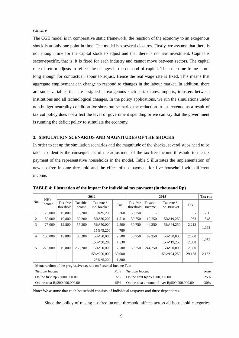
3. SIMULATION SCENARIOS AND MAGNITUDES OF THE SHOCKS

In order to set up the simulation scenarios and the magnitude of the shocks, several steps need to be

taken to identify the consequences of the adjustment of the tax-free income threshold to the tax

payment of the representative households in the model. Table 5 illustrates the implementation of

new tax-free income threshold and the effect of tax payment for five household with different

income.

TABLE 4: Illustration of the impact for Individual tax payment (in thousand Rp)

No. HH's

Income

2012 2013 Tax cut

Tax-free

threshold

Taxable

Income

Tax rate *

Inc. bracket Tax

Tax-free

threshold

Taxable

Income

Tax rate *

Inc. Bracket Tax

1 25,000 19,800 5,200 5%*5,200 260 30,750 -

- 260

2 50,000 19,800 30,200 5%*30,200 1,510 30,750 19,250 5%*19,250 963 548

3 75,000 19,800 55,200 5%*50,000 2,500 30,750 44,250 5%*44,250 2,213 1,068

15%*5,200 780

4 100,000 19,800 80,200 5%*50,000 2,500 30,750 69,250 5%*50,000 2,500

1,643

15%*30,200 4,530

15%*19,250 2,888

5 275,000 19,800 255,200 5%*50,000 2,500 30,750 244,250 5%*50,000 2,500

2,163

15%*200,000 30,000

15%*194,250 29,138

25%*5,200 1,300

Memorandum of the progressive tax rate on Personal Income Tax:

Taxable Income Rate Taxable Income Rate

On the first Rp50,000,000.00 5% On the next Rp250,000,000.00 25%

On the next Rp200,000,000.00 15% On the next amount of over Rp500,000,000.00 30%

Note: We assume that each household consists of individual taxpayer and three dependents.

Since the policy of raising tax-free income threshold affects across all household categories

10

and the progressive tax rate applies to the personal income tax so its impact will vary between

household categories, ceteris paribus. For example, household no. 2 experiences reducing the

taxable income from Rp30.2 million to Rp19.25 million. The level of income is in the bracket of

5% tax rate; resulting Rp0.548 million tax cut. While household no. 5, in the old tax-free income

threshold, has a taxable income of Rp255.2 million; subjects to three brackets of tax rate: 5%, 15%,

and 25%. In the new tax-free income threshold, the taxable income reduces to Rp244.25 million

and only subject to two brackets of tax rate: 5% and 15%. It means there is a portion of taxable

income shift from 25% to 15% income brackets; resulting a tax cut of Rp2.163 million.

In order to comparing the impacts with competing alternative policies, we also simulate three

different policies as shown at Table 5. In the policy simulations (SIM1, SIM2, and SIM3), we

estimate the level of tax cut in each percentile of household (rural and urban) as a result of raising

the tax-free income threshold policy. In addition, we also consider estimating the coverage ratio3 of

the personal income tax to have more reliable magnitude of the shocks. Even though in the last

decade the number of income tax payers has improved significantly but still concentrated into a

small portion of population as indicated by some studies such as Marks (2003), Ikhsan et al. (2005)

and Arnold (2012).

TABLE 5: Simulation scenarios

Simulation Description

SIM1 Increase tax-free income threshold as stipulated at Regulation No. 162/PMK.011/2012

SIM2 Tax-free income threshold eliminated but compensated with low level income tax offset

for the household with the level of income up to Rp50 million a year

SIM3 No adjustment on tax-free income threshold but reduces the marginal tax rate: from 30%

to 25%, from 25% to 18%; and from 15% to 14%.

SIM4 No adjustment on tax-free income threshold but government make a cash transfer of Rp1

million to the poor household each for the year

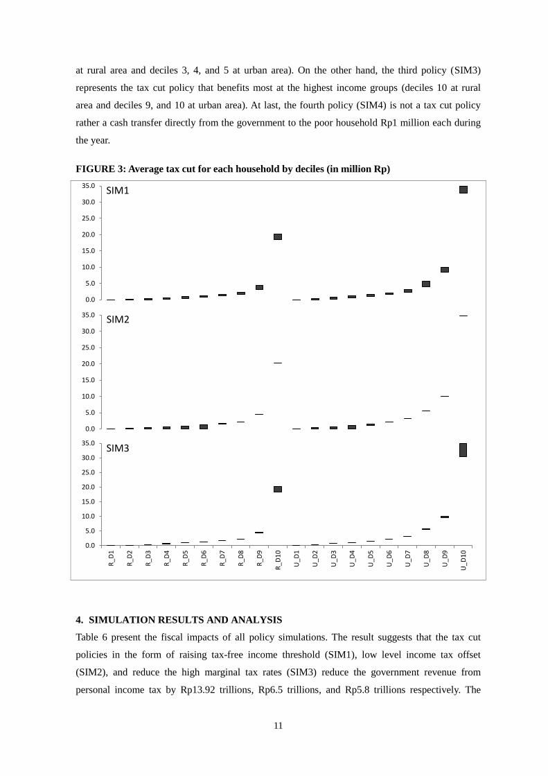
To illustrate the magnitude of shocks for SIM1, SIM2, and SIM3 across household income

level, Figure 3 shows the average tax cut for each household in the deciles category. As we can see

from the table, the first policy (SIM1) does not affect the first deciles of rural household, since the

income is still below the old tax-free income threshold. The 9th and 10th deciles in rural area and the

8th, 9th, and 10th deciles in urban area have higher tax-cut than others. The second policy (SIM2)

represents the closest policy but with the different approach. By design, SIM2 is better than SIM1

in term of attracting the lower income household groups to include in the tax system with the

incentive of tax offset (tax refund). Moreover, SIM2 and also creates better income redistribution as

shown at Figure 3 that the tax cut policy benefits most at lower income groups (deciles 3, 4, 5 and 6

3 Coverage ratio in here is defined as the actual income tax revenue collected by the government compare to

its potential in the economy.

11

at rural area and deciles 3, 4, and 5 at urban area). On the other hand, the third policy (SIM3)

represents the tax cut policy that benefits most at the highest income groups (deciles 10 at rural

area and deciles 9, and 10 at urban area). At last, the fourth policy (SIM4) is not a tax cut policy

rather a cash transfer directly from the government to the poor household Rp1 million each during

the year.

FIGURE 3: Average tax cut for each household by deciles (in million Rp)

4. SIMULATION RESULTS AND ANALYSIS

Table 6 present the fiscal impacts of all policy simulations. The result suggests that the tax cut

policies in the form of raising tax-free income threshold (SIM1), low level income tax offset

(SIM2), and reduce the high marginal tax rates (SIM3) reduce the government revenue from

personal income tax by Rp13.92 trillions, Rp6.5 trillions, and Rp5.8 trillions respectively. The

0.0

5.0

10.0

15.0

20.0

25.0

30.0

35.0SIM1

0.0

5.0

10.0

15.0

20.0

25.0

30.0

35.0SIM2

0.0

5.0

10.0

15.0

20.0

25.0

30.0

35.0

R_D

1

R_D

2

R_D

3

R_D

4

R_D

5

R_D

6

R_D

7

R_D

8

R_D

9

R_D

10

U_D

1

U_D

2

U_D

3

U_D

4

U_D

5

U_D

6

U_D

7

U_D

8

U_D

9

U_D

10

SIM3

12

decrease in personal income tax revenue is partially offset by an increase in the revenue from other

taxes: corporate income tax, indirect tax, and import tariff. It indicates that the raising tax-free

income threshold policy works well to stimulate the economy; indirect tax and import tariff sign for

household consumption and corporate income tax as a light of business profitability. The policy of

cash transfer to poor household (SIM4) is not tax cut policy but expenditure side policy and the

government need to allocate additional spending for it about Rp7.1 trillions. Cash transfer policy

also stimulates the economy as indicated by the increase in indirect tax, import tariff, personal

income tax, and corporate income tax.

TABLE 6: Fiscal impacts in each different simulation (in billion Rp)

SIM1 SIM2 SIM3 SIM4

Revenue Expend. Revenue Expend. Revenue Expend. Revenue Expend.

Indirect tax 790 0 301 0 584 0 237 0

Import tariffs 42 0 17 0 26 0 13 0

Personal Income Tax -13,917 0 -6,520 0 -5,779 0 51 0

Corporate Income Tax 1,175 0 427 0 893 0 326 0

Government consumption 0 2,636 0 965 0 2,030 0 733

Subsidies 0 385 0 147 0 269 0 116

Transfers from/to other inst. 4 538 1 200 3 388 1 7,111

Government saving (deficit) 0 -15,464 0 -7,087 0 -6,962 0 -7,332

TOTAL -11,906 -11,906 -5,774 -5,774 -4,274 -4,274 629 629

The macro economics impacts of the policy simulations, SIM1 to SIM4, are presented at

Table 7 – 10 respectively. The table summarised the impact of the policy to several aspects of

economy: (1) the supply side in the form of industrial output and price, (2) the demand side in the

form of real consumption by household deciles, (3) macro-economic variables, and (4) the impact

to the labour market in term of nominal wages and labour supply (employment).

As already mentioned before, the policy of raising tax-free income threshold (SIM1) works

well to stimulate the economy in the short-run scenario. As shown in Table 7, the real GDP

increases by 0.038 %. The source of growth is mainly from the increase in the household

consumption, accounted for 0.244%. An increase in demand creates the economy in inflationary

condition as reflected by an increase of CPI by 0.170%. It brings an impact of losing such level of

competitiveness for the export-oriented commodities. The real export decreases by 0.195%.

More detail impacts can be traced in the supply side of the economy. An increase in

disposable income as a result of tax cut policy increases the level of domestic consumption. The

excess demand in the economy creates a price increase and also an increase in production level. We

can see from Table 7 that nearly all commodities experience an increase in terms of price and

output. Government services, food-beverage-tobacco, livestock, and restaurant-hotel are example

13

for the sectors that highly driven by domestic consumption.

Furthermore, the increases in the level of production in the industrial sectors bring the

changes in the labour market. In the short-run scenario, we assume fixed capital (no new

investment) and fixed real wages. The changes in the labour market are transmitted into the

changes in the labour supply (employment) in the form of additional labour or working hours. The

changes in the nominal wages are merely adjustment of the inflation. From Table 7, we can link the

changes of the labour supply to the industrial output changes and the changes in the nominal wages

to the changes in the price of commodities. The variability of the changes is affected by some

factors such as the different preference of household consumption and the proportion of the factor

of production used in the production activities. As we can see that the significant changes in the

labour supply of management-professional (employee and self-employed) in the rural area are

related to the significant increase in the output of government services and the high proportion of

these type of labour in this sector in rural area (see again Table 2). In sum, the aggregate

employment increases by 0.057%.

TABLE 7: Results for SIM1 (% changes)

Supply side

Demand side

Supply Price

Income by deciles Rural Urban

Food crops 0.108 0.170

D_01 0.057 0.089

Other crops -0.002 0.115

D_02 0.247 0.460

Livestock 0.253 0.282

D_03 0.523 0.549

Forestry 0.024 0.185

D_04 0.581 0.451

Fishery 0.183 0.477

D_05 0.505 0.377

Coal-ore oil mining -0.018 -0.019

D_06 0.437 0.315

Other mining -0.001 0.149

D_07 0.381 0.480

Food-beverage-tobacco 0.274 0.146

D_08 0.328 0.616

Textile 0.164 0.041

D_09 0.605 0.477

Woods 0.186 0.090

D_10 0.427 0.315

Papers 0.152 0.064

Chemicals 0.080 0.014

Macro-variables

Electricity-gas-water 0.055 0.966

Real GDP 0.038 Real export -0.195

Constructions 0.005 0.122

Real consumption 0.244 Real import 0.042

Trade 0.038 0.187

Real investment 0.000 Aggregate employment 0.057

Restaurant-hotel 0.237 0.190

Real government 0.032 Average real wages 0.000

Road transportation 0.135 0.165

CPI 0.170 Average nominal wages 0.170

Air-water transportation 0.084 0.135

Transportation supports -0.037 0.140 Labour market

Nominal wages

Labour supply

Bank-finance 0.072 0.294

Rural Urban

Rural Urban

Real estate 0.074 0.381

Agri. Employee 0.294 0.336

1.176 4.475

Government services 0.409 0.229

Agri. Self-employed 0.278 0.316

0.396 3.865

Other services 0.191 0.231

Prod. Employee 0.152 0.141

0.699 0.371

Prod. Self-employed 0.127 0.173

1.169 1.284

Cler. Employee 0.266 0.240

1.675 0.353

Cler. Self-employed 0.125 0.145

1.025 0.679

Mgt. Employee 0.547 0.409

2.205 0.800

Mgt. Self-employed 0.255 0.277

12.505 4.689

14

The increase in the labour supply in turn brings an increase in the real domestic consumption

classified in the household deciles. The level of real household consumption changes are

combination of the changes in the labour supply as a result of policy response in the economy and

the initial impact of increasing the disposable income as a direct effect of tax cut policy. As shown

in Table 7, the impacts to the real consumption by deciles are varied. The 1st deciles household have

very small impacts for both in rural and urban areas. It is due to the 1st deciles are most likely have

no direct impacts from the raising tax-free income threshold policy.

Table 8 summarised the impacts of eliminating tax-free income threshold and replaced by the

low level income tax offset (SIM2). This policy is expected to have better impact on distributional

income. But the magnitudes of the tax cut are smaller or even less than half of SIM1, as shown at

Table 6. Therefore, we can see that the impact to the macro economy is relatively small, increase

in real household consumption only 0.09% and in economic growth only 0.013%.


Supply side

Demand side

Supply Price



D_01 0.021 0.054

Other crops 0.010 0.044

D_02 0.211 0.425


D_03 0.487 0.695


D_04 0.677 0.877

Fishery 0.065 0.170

D_05 0.816 0.394


D_06 0.947 0.008


D_07 0.120 0.007


D_08 0.021 0.007

Textile 0.074 0.018

D_09 0.021 0.008

Woods 0.060 0.033

D_10 0.021 0.009

Papers 0.043 0.020


Macro-variables





Trade 0.011 0.067

Real investment 0.000 Aggregate Employment 0.020







Nominal wages

Labour supply


Rural Urban

Rural Urban



0.403 1.516



0.136 1.312



0.239 0.127


0.400 0.439


0.573 0.121


0.351 0.233


0.753 0.274


4.132 1.587

As expected, the policy has good impact on the distribution of income. From the demand

side impacts, we can see that the household income increases and the lower income household i.e.

15

deciles 2-7 (rural) and deciles 2-5 (urban) experienced relatively high increase in the income. While

other deciles group only benefited from indirect impacts that relatively small. It is noteworthy that

this policy also only has indirect impact to the poorest household groups, deciles 1 and part of

deciles 2 at rural area and part of deciles 1 at urban area. It is because these household categories

are not income tax payers due to the income still below the threshold.

The changes in the demand side bring the changes in the supply side of economy. The output

of food, beverages and tobacco increase significantly. It follows by other agricultural commodities

that highly related with low-middle income type consumption in Indonesia. It is also confirmed by

the impact in the labour market which the higher impacts are on those related industries.

On the other hand, Table 9 represent the impact of the policy that benefit only the high level

income household by reducing the high marginal tax rates (SIM3). Even though the cost of the tax

cut for this policy is smaller than SIM2, but the impact to the economy is higher; as indicated by

real household consumption and real GDP that could grow by 0.189% and 0.037% respectively.

The factors that may affect this impact need to address further.


Supply side

Demand side

Supply Price



D_01 0.052 0.067

Other crops -0.024 0.082

D_02 0.052 0.065


D_03 0.052 0.063

Forestry -0.006 0.087

D_04 0.051 0.060

Fishery 0.091 0.262

D_05 0.050 0.058


D_06 0.049 0.055


D_07 0.049 0.079


D_08 0.048 0.133

Textile 0.078 0.022

D_09 0.088 0.191

Woods 0.156 0.069

D_10 0.215 0.494

Papers 0.147 0.056


Macro-variables





Trade 0.046 0.145








Nominal wages

Labour supply


Rural Urban

Rural Urban



1.214 4.625



0.409 3.994



0.721 0.383


1.206 1.325


1.729 0.364


1.058 0.701


2.278 0.826


12.935 4.844

16

In term of distributional income effect, the policy (SIM3) affects significant income increase

of the household at deciles 9-10 (rural) and deciles 7-10 (urban) with the highest impacts in the top

deciles and decreasing to the lowers. Other deciles experiences only indirect impact of the policy.

But we can see that the indirect impact of SIM3 is higher than SIM2 even though with the lower

value of tax cut. It indicates that tax cut policy at high level income household group has higher

impact than at low level income household group.

The impact of policy SIM3 at supply side is related to middle-high income household. As

shown at Table 9 that restaurant and hotel experienced the highest increase in output; not food,

beverages, and tobacco. Restaurant and hotel is classified as consumption type that highly related

with middle-high income household.

In contrast with three previous policies, SIM4 is not tax cut policy but direct cash transfer

from the government to the poor household. It has similar effect to stimulate the economy, the real

household consumption increases by 0.069% to make the overall economy to grow at 0.010%.

Even though the value of the cash transfer is a bit higher than the value of tax cut at SIM2 and

SIM3 but the level of impact on the economy is smaller.


Supply side

Demand side

Supply Price



D_01 5.553 4.446

Other crops 0.018 0.036

D_02 1.983 0.002


D_03 0.018 0.002


D_04 0.018 0.002

Fishery 0.037 0.106

D_05 0.018 0.003


D_06 0.019 0.003


D_07 0.019 0.003


D_08 0.019 0.003

Textile 0.053 0.014

D_09 0.020 0.004

Woods 0.023 0.020

D_10 0.020 0.005

Papers 0.025 0.014


Macro-variables





Trade 0.008 0.053








Nominal wages

Labour supply


Rural Urban

Rural Urban



0.315 1.187



0.107 1.027



0.188 0.100


0.313 0.344


0.449 0.095


0.275 0.183


0.590 0.215


3.225 1.242

17

The advantage of cash transfer policy is that it target to the poor household directly. As we

can see from Table 10, the real income of poor households (deciles 1-2 at rural and deciles 1 at

urban) increases significantly while others only have relatively small (indirect) impacts. In

addition, the impacts of the cash transfer policy to the supply side of economy and labour market

are relatively similar to the impacts of SIM2 (tax cut at low level income households).

5. CONCLUDING REMARKS AND FURTHER RESEARCH

In this paper, the integrated multi-household CGE model is used to simulate the distributional

welfare impact of the raising tax-free income threshold in Indonesia that started to implement on

1st January 2013. The model database is consolidated from Indonesia IO, SAM, and Susenas for

the year of 2008. The model has 200 household categories to represent the percentile household

income distribution in two different areas: rural and urban. Four scenarios of the policy are

evaluated, not only increasing tax-free income threshold but also three competing alternative

policies: (1) eliminating the tax-free income threshold and replaced by low income tax offset, (2)

reducing the higher marginal tax rates, and (3) giving cash transfer to poor households.

The results suggest that the policy of increasing tax-free income threshold (SIM1) could

increase the economic welfare as shown in aggregate by the increase in real GDP growth and real

household consumption. It concludes that raising the tax-free income threshold policy work well to

stimulate the economic growth.

In terms of distributional welfare impact, we find that the magnitude of impacts are varies

across the household categories. The distributional welfare impact is affected by direct and indirect

impact of the policy to the household disposable income or consumption. The direct impact in the

form of tax cut is a product of the household income levels and the progressive rate in the

Indonesia income tax system. On the other hand, the magnitude of indirect impact is defined by the

structure of the economy such as the characteristics of household consumption and the proportion

of the factor of production in each economic activity. The structure of economy is characterised by

the database, set of parameters, and the equation system in the CGE model.

Unfortunately, the lowest household income deciles only have very small increase in the

impact of real consumption for both rural and urban areas. Even though the raising tax-free income

threshold affects across all tax payers, all household categories but the household with higher

income benefited more.

By comparing the result of the policy to three competing alternatives, we can conclude as

follows:

(1) Three competing alternative policies also have a good effect to stimulate the economy with

varies magnitude of impacts.

(2) The policy of eliminating the tax-free income threshold and replacing with low level income

offset (SIM2) has better distributional impact since the policy limits to the low level income

18

household groups. But still the poor households only have benefit from very small (indirect)

impact since they are not tax payers.

(3) The policy of reducing high marginal tax rates or tax cut at high income household groups

(SIM3) give higher impact on fostering economic growth but relatively small (indirect)

impacts to the lower income household groups.

(4) The policy of cash transfer (SIM4) is the best to target the poor but only give relatively small

impact to the growth.

In term of policy implementation, the tax cut policies (SIM1, SIM2, and SIM3) are easy to

be applied since the tax system and administration already in place, but cash transfer policy (SIM4)

need such additional cost to administer the operational. The policy of using low level income tax

offset (SIM2) brings a good opportunity to extend the coverage of tax payers from low-middle

income. This policy will attract these household groups to enter the tax system. It will address the

current issue of only small portion of population that already registered and actively contribute as

tax payers. Then, the policy of tax cut at high income household groups (SIM3) may be fit at crisis

situation. If we can combine the cash transfer policy (SIM4) in the tax system, it will reduce the

cost administration. Although to do so, it needs hard work to cover low-middle income households

to the tax system particularly for the households in rural area. But it is worth in the long-run, not

only to improve the tax system and administration but also to make better environment to combine

wider alternatives of tax policy that fit best to the objectives such as redistribution of income and

fostering economic growth.

There are many possible ways the study could be extended. First, further research could

analyse the effect of raising the tax-free income threshold in the regional CGE model framework.

Indonesia economy diversifies into many regions with different characteristics, particularly in the

distributional household income and the factor production composition. As we all know that

assessing the impact in the regional level will give more flavour in the economic development

policies rather than in the national level.

Second, the simulations are only focusing on the raising tax-free income threshold policy.

Usually in the policy implementation, the adjustment of the tax-free income threshold will

complemented by the increase in the minimum labour wages that effective by regions in Indonesia.

In addition of the methodological approach in the regional modelling framework, it is also

necessary to evaluate the combination policy of the adjustment of the tax-free income threshold and

provincial/district minimum labour wages.

References

Abdurohman, and Resosudarmo, B. (2012). Economy-wide Impacts of the 2009 Fiscal Stimulus

19

Package in Indonesia. Paper presented at the 11th Indonesia Regional Science Association

(IRSA) International Conference.

Amir, H. (2011). Tax Policy, Growth, and Income Distribution in Indonesia: A Computable

General Equilibrium Analysis. Unpublished PhD Thesis, The University of Queensland,

Brisbane.

Amir, H., et al. (2013). The impact of the Indonesian income tax reform: A CGE analysis.

Economic Modelling, 31, 492-501.

Armington, P. S. (1969). Theory of Demand for Products Distinguished by Place of Production.

IMF Staff Paper, 16(1), 159 - 178.

Arnold, J. (2012). Improving the tax system in Indonesia, Economics Department Working Papers

No. 998. OECD: Organisation for Economic Co-operation and Development.

Atuesta, L., and Hewings, G. J. D. (2012). Economic welfare analysis of the legalization of drugs: a

CGE microsimulation model for Colombia. Economic Systems Research, iFirst 2012, 1-22.

Creedy, J., et al. (2008). Abolishing the Tax-Free Threshold in Australia: Simulating Alternative

Reforms, Working Paper in Department of Economics No. 1048. Melbourne: University of

Melbourne.

Dixon, P. B., et al. (1982). ORANI: A Multisectoral Model of Australian Economy. Amsterdam:

North-Holland.

Dixon, P. B., and Rimmer, M. T. (2002). Dynamic General Equilibrium Modelling for Forecasting

and Policy: A Practical Guide and Documentation of MONASH. Amsterdam: North

Holland.

Horridge, J. M. (2003). ORANI-G: A Generic Single-Country Computable General Equilibrium

Model. Retrieved 22 April 2009, from http://www.monash.edu.au/policy/oranig.htm

Ikhsan, M., et al. (2005). Indonesia's New Tax Reform: Potential and Direction. Journal of Asian

Economics, 16, 1029 - 1046.

Marks, S. V. (2003). Personal Income Taxation in Indonesia: Revenue Potential and Distribution of

the Burden. Jakarta: Bappenas.

Saunders, P. (2006). Taxploitation: The Case for Income Tax Reform. Sydney: Centre for

Independent Studies.

Wittwer, G. (1999). WAYANG: a General Equilibrium Model Adapted for the Indonesian Economy.

Adelaide: Centre for International Economic Studies, University of Adelaide.

Yusuf, A. A. (2007). Constructing Indonesian Social Accounting Matrix for Distributional Analysis

in the CGE Modelling Framework. MPRA Paper No. 1730.

Yusuf, A. A., et al. (2008). AGEFIS: Applied General Equilibrium for FIScal Policy Analysis.

Bandung: Center for Economics and Development Studies, Department of Economics,

Padjadjaran University.

http://www.monash.edu.au/policy/oranig.htm

Documents

Munich Personal RePEc Archive · A tax-free income threshold (Penghasilan Tidak Kena Pajak/PTKP; Bahasa Indonesia) ... 2011). The 2008 Indonesian SAM is a single output type industry,