Multivariate Spatial Process Gradients with Environmental

Multivariate Spatial Process Gradients with

Environmental Applications

by

Maria A. Terres

Department of Statistical ScienceDuke University

Date:Approved:

Alan E. Gelfand, Supervisor

Robert L. Wolpert

Mine Cetinkaya-Rundel

James S. Clark

Dissertation submitted in partial fulfillment of the requirements for the degree ofDoctor of Philosophy in the Department of Statistical Science

in the Graduate School of Duke University2014

Abstract

Multivariate Spatial Process Gradients with Environmental

Applications

by

Maria A. Terres

Department of Statistical ScienceDuke University

Date:Approved:

Alan E. Gelfand, Supervisor

Robert L. Wolpert

Mine Cetinkaya-Rundel

James S. Clark

An abstract of a dissertation submitted in partial fulfillment of the requirements forthe degree of Doctor of Philosophy in the Department of Statistical Science

in the Graduate School of Duke University2014

Copyright c© 2014 by Maria A. TerresAll rights reserved except the rights granted by the

Creative Commons Attribution-Noncommercial Licence

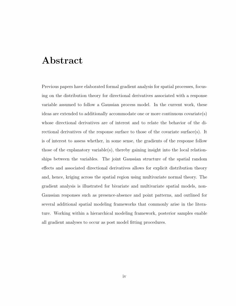
http://creativecommons.org/licenses/by-nc/3.0/us/

Abstract

Previous papers have elaborated formal gradient analysis for spatial processes, focus-

ing on the distribution theory for directional derivatives associated with a response

variable assumed to follow a Gaussian process model. In the current work, these

ideas are extended to additionally accommodate one or more continuous covariate(s)

whose directional derivatives are of interest and to relate the behavior of the di-

rectional derivatives of the response surface to those of the covariate surface(s). It

is of interest to assess whether, in some sense, the gradients of the response follow

those of the explanatory variable(s), thereby gaining insight into the local relation-

ships between the variables. The joint Gaussian structure of the spatial random

effects and associated directional derivatives allows for explicit distribution theory

and, hence, kriging across the spatial region using multivariate normal theory. The

gradient analysis is illustrated for bivariate and multivariate spatial models, non-

Gaussian responses such as presence-absence and point patterns, and outlined for

several additional spatial modeling frameworks that commonly arise in the litera-

ture. Working within a hierarchical modeling framework, posterior samples enable

all gradient analyses to occur as post model fitting procedures.

iv

Dedicated to all of the formal and informal teachers I’ve had along the way.

v

Contents

Abstract iv

List of Tables x

List of Figures xi

List of Abbreviations and Symbols xiii

Acknowledgements xv

1 Introduction 1

1.1 Geostatistical Modeling and Gaussian Processes . . . . . . . . . . . . 1

1.1.1 The Basics of Geostatistical Modeling . . . . . . . . . . . . . . 1

1.1.2 More Advanced Geostatistical Modeling . . . . . . . . . . . . 3

1.2 Spatial Modeling for Environmental Applications . . . . . . . . . . . 6

1.3 Spatial Gradient Processes . . . . . . . . . . . . . . . . . . . . . . . . 6

1.4 Thesis Contribution and Outline . . . . . . . . . . . . . . . . . . . . . 8

2 Bivariate Spatial Gradients 12

2.1 Introduction . . . . . . . . . . . . . . . . . . . . . . . . . . . . . . . . 12

2.2 Distribution Development . . . . . . . . . . . . . . . . . . . . . . . . 14

2.3 Model Fitting and Inference . . . . . . . . . . . . . . . . . . . . . . . 19

2.3.1 Sampling Method . . . . . . . . . . . . . . . . . . . . . . . . . 19

2.3.2 Local Directional Sensitivity Process . . . . . . . . . . . . . . 21

2.3.3 Spatial Angular Discrepancy Process . . . . . . . . . . . . . . 24

vi

2.4 Simulation Example . . . . . . . . . . . . . . . . . . . . . . . . . . . 27

2.4.1 Data and Model . . . . . . . . . . . . . . . . . . . . . . . . . . 28

2.4.2 Local Directional Sensitivity Process . . . . . . . . . . . . . . 29

2.4.3 Spatial Angular Discrepancy Process . . . . . . . . . . . . . . 31

2.5 Summary . . . . . . . . . . . . . . . . . . . . . . . . . . . . . . . . . 31

3 Gradient Analysis for Non-Gaussian Responses 34

3.1 Introduction . . . . . . . . . . . . . . . . . . . . . . . . . . . . . . . . 34

3.2 Extensions to Non-Gaussian Data Models Using the Chain Rule . . . 35

3.3 Spatial Generalized Linear Models . . . . . . . . . . . . . . . . . . . . 36

3.4 South Africa Protea, Elevation Analysis . . . . . . . . . . . . . . . . 44

3.4.1 Cape Floristic Region Data . . . . . . . . . . . . . . . . . . . 44

3.4.2 Binomial Model and Spatial Gradients . . . . . . . . . . . . . 45

3.4.3 Results . . . . . . . . . . . . . . . . . . . . . . . . . . . . . . . 48

3.5 Duke Forest Point Pattern, Elevation Analysis . . . . . . . . . . . . . 50

3.5.1 Duke Forest Data . . . . . . . . . . . . . . . . . . . . . . . . . 50

3.5.2 Point Pattern Model and Spatial Gradients . . . . . . . . . . . 51

3.5.3 Results . . . . . . . . . . . . . . . . . . . . . . . . . . . . . . . 53

3.6 Summary . . . . . . . . . . . . . . . . . . . . . . . . . . . . . . . . . 56

4 Gradient Analysis for Multivariate Spatial Processes 59

4.1 Introduction . . . . . . . . . . . . . . . . . . . . . . . . . . . . . . . . 59

4.2 Modeling Development . . . . . . . . . . . . . . . . . . . . . . . . . . 61

4.2.1 Multiple Predictors . . . . . . . . . . . . . . . . . . . . . . . . 61

4.2.2 Multiple Responses . . . . . . . . . . . . . . . . . . . . . . . . 67

4.2.3 Multiple Responses and Predictors . . . . . . . . . . . . . . . 70

4.3 Multivariate Examples using South African Plant Traits . . . . . . . 72

vii

4.3.1 Data . . . . . . . . . . . . . . . . . . . . . . . . . . . . . . . . 72



4.4 Results . . . . . . . . . . . . . . . . . . . . . . . . . . . . . . . . . . . 75



4.5 Summary . . . . . . . . . . . . . . . . . . . . . . . . . . . . . . . . . 80

5 Additional Gradient Analysis Extensions 83

5.1 Spatial-Temporal Modeling . . . . . . . . . . . . . . . . . . . . . . . . 83

5.1.1 Introduction . . . . . . . . . . . . . . . . . . . . . . . . . . . . 83

5.1.2 Modeling and Gradient Theory . . . . . . . . . . . . . . . . . 84

5.2 Data with Spatial Misalignment . . . . . . . . . . . . . . . . . . . . . 87

5.2.1 Introduction . . . . . . . . . . . . . . . . . . . . . . . . . . . . 87


5.3 Spatially Varying Coefficient Processes . . . . . . . . . . . . . . . . . 93

5.3.1 Introduction . . . . . . . . . . . . . . . . . . . . . . . . . . . . 93


5.4 Predictive Process Model . . . . . . . . . . . . . . . . . . . . . . . . . 96

5.4.1 Introduction . . . . . . . . . . . . . . . . . . . . . . . . . . . . 96


5.5 Total Derivative . . . . . . . . . . . . . . . . . . . . . . . . . . . . . . 100

5.5.1 Introduction . . . . . . . . . . . . . . . . . . . . . . . . . . . . 100


A Bivariate Gradient Theory 103

A.1 Spatial Cauchy Process . . . . . . . . . . . . . . . . . . . . . . . . . . 103

viii

A.2 Bivariate Angular Density . . . . . . . . . . . . . . . . . . . . . . . . 106

Bibliography 108

Biography 113

ix

List of Tables

2.1 Parameter estimates for the [Y (s)|X(s)][X(s)] model. . . . . . . . . . 29

3.1 Parameter estimates for the [Y (s)|X(s)][X(s)] model. . . . . . . . . . 48

3.2 Parameter estimates for [X(s)] model for elevation. . . . . . . . . . . 54

3.3 Parameter estimates for [Z(s)|X(s)] model for Flowering Dogwood. . 55

3.4 Parameter estimates for [Z(s)|X(s)] model for Sweetgum. . . . . . . . 55

4.1 Parameter estimates and 95% credible intervals for the [Y |X1, X2][X1, X2]model. . . . . . . . . . . . . . . . . . . . . . . . . . . . . . . . . . . . 76

4.2 Parameter estimates and 95% credible intervals for the [Y1, Y2|X][X]model. . . . . . . . . . . . . . . . . . . . . . . . . . . . . . . . . . . . 79

x

List of Figures

2.1 Bivariate density for (θX(s), θY (s)) at a fixed s for varying values ofβ. All other parameters are set to the values used for simulation inSection 2.4. . . . . . . . . . . . . . . . . . . . . . . . . . . . . . . . . 27

2.2 X(s) (left) and Y (s) (right) subregions around s∗, where we estimatethe gradient. . . . . . . . . . . . . . . . . . . . . . . . . . . . . . . . . 29

2.3 Posterior median of DuY (s)/DuX(s) in the directions u = (1, 0) (left)and u = (0, 1) (right). . . . . . . . . . . . . . . . . . . . . . . . . . . 31

2.4 Posterior median disc(s). . . . . . . . . . . . . . . . . . . . . . . . . . 32

3.1 Centroids of observed areal units (left), interpolated Y (s)/N(s) sur-face (center) and interpolated X(s) surface (right). . . . . . . . . . . 45

3.2 Posterior mean P (s) surface. . . . . . . . . . . . . . . . . . . . . . . . 49

3.3 Posterior medianDuP (s)/DuX(s) for u North/South (left) and East/West(right). . . . . . . . . . . . . . . . . . . . . . . . . . . . . . . . . . . . 49

3.4 Posterior median disc(s) = 1− cos(θX(s)− θP (s)). . . . . . . . . . . 50

3.5 From left to right, observed point patterns for Flowering Dogwoodand Sweetgum and observed elevation. . . . . . . . . . . . . . . . . . 51

3.6 Posterior median of the intensity surface for Flowering Dogwood (left)and Sweetgum (right). . . . . . . . . . . . . . . . . . . . . . . . . . . 54

3.7 Posterior median of Duλ(s)/DuX(s) for Flowering Dogwood (left) andSweetgum (right); u = (0.8508,−0.5255). . . . . . . . . . . . . . . . . 55

3.8 Posterior median disc(s) for Flowering Dogwood (left) and Sweetgum(right). . . . . . . . . . . . . . . . . . . . . . . . . . . . . . . . . . . . 56

4.1 Plot locations for Cape Floristic Region leaf trait data. . . . . . . . . 73

4.2 Plant trait variables (top row) and climate variables (bottom row). . 74

xi

4.3 Posterior mean kriged surfaces for X1(s), X2(s), and µ(s) from left toright. . . . . . . . . . . . . . . . . . . . . . . . . . . . . . . . . . . . . 76

4.4 Top row: Posterior median local sensitivity surfaces; Duµ(s)/DuX1(s)andDuµ(s)/DuX2(s). Bottom row: Posterior median angular discrep-ancy surfaces; disc1(s) and disc2(s). . . . . . . . . . . . . . . . . . . . 77

4.5 Posterior mean kriged surfaces for X, µ1, and µ2 from left to right. . 78

4.6 Top row: Posterior median local sensitivity surfaces; Duµ1(s)/DuX(s)and Duµ2(s)/DuX(s). Bottom row: Posterior median angular dis-crepancy surfaces; disc1(s), disc2(s). . . . . . . . . . . . . . . . . . . 80

xii

List of Abbreviations and Symbols

Symbols

Rd Set of all d-dimensional real-valued vectors.

N(m, v) Multivariate normal with mean m and covariance matrix v.

E(x) Expected value of x.

V ar(x) Variance of x.

SD(x) Standard deviation of x.

Cov(x, y) Covariance of x and y.

Φ(x) Standard normal cdf evaluated at x.

φ(x) Standard normal pdf evaluated at x.

Abbreviations

CAR Conditionally autogregressive.

CDF Cumulative distribution function.

CFR Cape Floristic Region.

FWC Leaf fresh water content.

GLM Generalized linear model.

GP Gaussian process.

GPS Global positioning system.

GWR Geographically weighted regression.

LMA leaf dry mass per unit area.

xiii

MAP Mean annual precipitation.

MAT Mean annual temperature.

MCMC Markov chain Monte carlo.

PDF Probability density function.

SVCP Spatially varying coefficient process.

xiv

Acknowledgements

I would like to thank my advisor, Alan Gelfand, for his encouragement and support

over the past few years. Our many discussions spanning past, present and future

have undoubtedly shaped my career and life as a statistical researcher. I am grateful

to Jim Clark and the other members of the CDI group for engaging discussions each

week. I am appreciative of Robert Wolpert who was always available to hear my

joys and concerns, as well as Mine Cetinkaya-Rundel, Kari Lock-Morgan and Dalene

Stangl for supporting my summer teaching endeavors. Finally, a big thank you to

my friends and family for believing in me.

In addition, I would like to acknowledge National Science Foundation (NSF),

International Society for Bayesian Analysis (ISBA), American Statistical Association

(ASA), Commonwealth Scientific and Industrial Research Organisation (CSIRO) and

Duke University for providing financial support of my education.

xv

1

Introduction

1.1 Geostatistical Modeling and Gaussian Processes

1.1.1 The Basics of Geostatistical Modeling

Due in part to advances in various technologies, such as Global Positioning Systems

(GPS), recording geocoded locations has become a routine aspect of data collection.

Such data allow for exploratory and statistical investigation into how the outcome

of interest behaves across different spatial regions. While covariate information may

explain a substantial portion of the variation in response, there is often underlying

spatial structure that is difficult to account for and may bias results if ignored. To

accommodate the abundance of geo-referenced data, spatial process models have

become widespread and are outlined in detail in several articles and books (e.g.

Banerjee et al., 2004; Cressie and Wikle, 2011). While spatial modeling is appropriate

in a variety of contexts, the examples and applications explored throughout this text

will be focused on ecology and the environment.

For a region of interest D, the set of conceptual responses Y (s) : s ∈ D can be

viewed as a realization of a random surface observed at a finite set of locations. The

1

general model for such data is of the form,

Y (s) = µ(s) + w(s) + ε(s) (1.1)

where µ(s) is a location-specific mean generally modeled as a linear function of some

covariates, ε(s) is a pure error term modeled as a zero-mean white noise process, and

w(s) is a spatial error term modeled as a zero-mean stationary Gaussian process.

For some data, such as elevation, the spatial-error term may be sufficient and ε(s)

will be removed from the model.

A spatial process with density p(·) is defined over any set of locations s1, . . . , sn

such that p(s1, . . . , sn) is consistent across permutations and marginalizations. If the

process is Gaussian, then the associated density will be multivariate normal and

characterized by a covariance function, c(·). A valid covariance function must be a

positive definite function, and may exhibit additional properties such as stationarity

and isotropy. A process is strictly stationary when p(s1, . . . , sn) = p(s1+δ, . . . , sn+δ)

for some separation vector δ, and it is weakly stationary when µ(s) = µ for all s and

Cov(Y (s), Y (s + δ)) = c(δ). A Gaussian process is weakly stationary if and only if

it is strictly stationary, so throughout this text we will refer to processes as simply

“stationary”. A stationary covariance function is isotropic if it depends only on the

length of the separation vector δ, c(δ) = c(||δ||).

The Gaussian processes illustrated in the following chapters will typically be

mean-zero with stationary isotropic covariance functions. In particular we focus on

the flexible class of Matern covariance functions with mean square differentiability

of process realizations controlled by a smoothness parameter ν. In our examples it

is desirable to have once, but not twice, mean square differentiability, so the Matern

covariance with ν = 3/2 is selected: c(||δ||) = σ2(1 + φ||δ||) exp(−φ||δ||).

A hierarchical Bayesian approach is used to fit the model in (1.1). Letting

Y = (Y (s1), . . . , Y (sn))′ represent the observed responses, W = (W (s1), . . . ,W (sn))′

2

represent the associated spatial random effects, and X be the matrix of covariates,

the model can be written

Y|W,θ ∼ N(Xβ + W, τ 2) (1.2)

W|θ ∼ N(0, K(·|σ2, φ))

p(θ) = p(β)p(τ 2)p(σ2)p(φ)

where K(·|σ2, φ) is a covariance matrix with entry i, j evaluated at δ = si − sj,

and p(θ) is the prior on the model parameters. The model is fit using MCMC

methods, and to improve fitting one would generally marginalize over the spatial

random effects W when fitting this model. However, marginalization will not be

possible when the first-stage is non-Gaussian; instead, the spatial random effects will

need to be sampled at each iteration.

While data is only observed at a finite set of locations, e.g. pollution concentra-

tions measured at monitoring stations, researchers are generally interested in how the

data varies across the entire region including unobserved locations. One advantage

of the spatial model described above is that it enables straight forward prediction at

unobserved locations, also known as kriging. This interpolation takes place via the

posterior predictive distribution. For an unobserved location s0,

p(Y (s0)|X(s0),Y,X) =

∫p(Y (s0)|X(s0),Y,θ)p(θ|Y,X)dθ

with samples Y (s0) drawn from p(Y (s0)|X(s0),Y,X) via composition. For a Gaus-

sian first-stage p(Y (s0)|X(s0),Y,θ) is easily computed using multivariate normal

theory.

1.1.2 More Advanced Geostatistical Modeling

Spatial modeling goes well beyond the spatial linear model defined in (1.1), with

modifications enabling application to a wide variety of problems and datasets. Ex-

amples of such extensions include multivariate spatial models, spatial models for

3

non-Gaussian responses, spatial-temporal models, spatially-varying coefficient mod-

els, and several adaptations to improve computational efficiency for large datasets.

These topics are briefly reviewed here.

When there are several variables of interest whose surfaces can all reasonably

be assumed to be spatially smooth their behavior can be captured through a joint

spatial model. Several frameworks exist for multivariate spatial modeling including

some simple separable models as well as more constructive non-separable approaches.

In our demonstrations we focus on the coregionalization model which can either be

built through successive conditioning of the variables or through specification of a

joint dependence on latent Gaussian processes (Royle and Berliner, 1999; Banerjee

et al., 2004). Within this framework there will be an equal number of latent Gaussian

processes and spatial variables, although each spatial variable may be dependent on

multiple Gaussian processes to induce dependence between the variables.

For some applications the response variable of interest cannot be assumed to

follow a normal distribution. For example, presence-absence observations for a plant

or animal species correspond to a binary response, making a binomial distribution a

more appropriate first-stage in (1.2). In general, a spatial generalized linear model

(GLM) can be fit for these types of non-Gaussian data (e.g. Heagerty and Lele,

1998; Paciorek, 2007; Berrett and Calder, 2012). These spatial GLMs utilize a link

function to relate a latent Gaussian process and a continuous response, such as

presence probability. As in the standard spatial process model, the latent Gaussian

process encourages similar outcomes for proximate locations.

Many environmental quantities are available at a fine temporal scale, e.g. daily

pollutant levels, indicating a need for combined spatial-temporal modeling. Similar

to the multivariate scenario, these models may be separable treating space and time

as independent, or may be non-separable. Generally the non-separable models will

be preferable, since space and time are often expected to interact. Spatial-temporal

4

models have been laid out in several books, (e.g. Wikle et al., 1998; Banerjee et al.,

2004; Cressie and Wikle, 2011), and have been adapted and extended in the literature,

(e.g. Gelfand et al., 2005; Reich et al., 2011b). These models allow for examination

of temporally-varying spatial relationships between variables.

To allow for spatially varying relationships between variables one can fit a spa-

tially varying coefficient model. The most common approaches for such models are

the spatially varying coefficient process (SVCP) proposed by Gelfand et al. (2003)

and the geographically weighted regression (GWR) proposed by Fotheringham et al.

(2002). The former is a Bayesian model in which regression coefficients are treated

as spatially correlated processes, while the latter estimates parameters using spatial

weights to emphasize proximate observations. Comparing the relative benefits of

the two models, simulation studies suggest the coefficient estimates under SVCP are

more accurate and more robust to collinearity than GWR and provides more for-

mal measures of model uncertainty (Wheeler and Calder, 2007; Wheeler and Waller,

2009). However, both models can be computationally intensive, and make assump-

tions regarding the variables’ relationship that go beyond a standard spatial regres-

sion model.

With the above as examples, there is clearly a wide array of spatial modeling

techniques that accommodate many types of data and allow for flexible relationships

between variables. However, many of these models suffer from long computation

times when subjected to large datasets common for environmental applications. The

primary computational expenses are the high-dimensional matrix decompositions re-

lated to the covariance matrix in the Gaussian process model. Recent approaches

for reducing computation times generally favor working in a lower dimensional sub-

space to approximate the full likelihood (e.g. Wikle and Cressie, 1999; Higdon, 2002;

Ver Hoef et al., 2004; Kim et al., 2005; Fuentes, 2007; Banerjee et al., 2008; Stein,

2013). Each approximation corresponds to a unique set of advantages and disadvan-

5

tages, but all share the common goal of speeding up computation time to accommo-

date large spatial data.

1.2 Spatial Modeling for Environmental Applications

Environmental data are increasingly collected across large spatial regions and are

recorded with geo-referenced locations. Examples of environmental point-referenced

data include pollutant levels, temperature, elevation and, when the spatial scale is

large enough, plot-level ecological data such as species presence. In recent years

the environmental literature has seen arguments in favor of Bayesian hierarchical

modeling for both spatial and non-spatial data (Clark, 2005; Clark and Gelfand,

2006; Cressie et al., 2009). The complex systems within which environmental and

ecological variables interact make the Bayesian treatment of uncertainty an appealing

and realistic framework. Similarly, accounting for unmeasured spatial variation can

improve model inference and allow for interpolation across the region. Examples of

spatial models for environmental applications are abundant in the literature including

capture-recapture data (Royle et al., 2013), pollution levels (Reich et al., 2011a),

tropical tree growth (Baribault et al., 2012), among many others.

1.3 Spatial Gradient Processes

Spatial gradients under Gaussian processes were elaborated in Banerjee et al. (2003)

to address the rate of change of a spatial surface at a given point in a given direction.

Their paper defines directional derivative processes with corresponding distribution

theory to enable interpolation across a region. For a mean square differentiable

process Y (s), they define the directional derivative in the direction u as

DuY (s) = limh→0

Y (s + hu)− Y (s)

h(1.3)

6

For a spatial process defined in R2, the gradient vector is defined in the directions

forming an orthonormal basis: ∇Y (s) = (De1Y (s), De2Y (s))′ where ei is a 2×1 vector

of 0s with a 1 in the ith entry. For any direction of interest u, the directional derivative

can be computed using the gradient vector, DuY (s) = u′∇Y (s). Jointly with the

parent Y (s) process, the gradient vectors follow a multivariate Gaussian process with

distribution fully determined by parameters in the parent spatial model, [Y (s)|θ].

Thus, computing the posterior predictive distribution for ∇Y (s)|Y (s) is simply an

application of multivariate normal theory, and posterior draws of the gradient vectors

can occur via composition using the posterior samples of the parameters for the

parent model. As such, all gradient analysis occurs post model fitting.

Subsequent papers addressed the smoothness of the gradient processes (Baner-

jee and Gelfand, 2003), applied the methodology to models with spatially varying

coefficients (Majumdar et al., 2006), extended the methods to allow for curvilinear

or boundary analysis (Banerjee and Gelfand, 2006), and explored analysis for non-

Gaussian spatial processes, in particular, the spatial Dirichlet processes (Guindani

and Gelfand, 2006). All of the current literature on spatial gradient processes focuses

on the rates of change of a response surface, with the mean surface modeled as a

linear function of a set of fixed covariates.

Spatial gradient processes can be helpful in illuminating environmental patterns

across spatial regions. For example, ecologists are interested in characterizing how

plants’ range boundaries relate to climate (e.g. Canham and Thomas, 2010; Thuiller

et al., 2004; Thomas, 2010). One aspect of this may be to consider the rate of change

for plant frequencies along a temperature gradient. These kinds of studies can provide

insight into potential effects of climate change on plants’ range distributions.

7

1.4 Thesis Contribution and Outline

Consider a response-covariate pair measured within a spatial region. Particularly

within the complex context of environmental and ecological data, it is unlikely that

the covariate will have a uniform effect on the response variable across the entire

region. Instead there may be pockets where the covariate has a negative influence,

pockets where it has a positive influence, and/or pockets where it has a negligible

influence. Possible explanations for such variation in the relationship include spatial

variation in unaccounted for covariates, the magnitude of the response or covariate, or

the rate of change of the response or covariate. Examination of how this relationship

is varying spatially is a desirable alternative to painstakingly trying to model every

possible explanatory factor.

One approach to understanding spatially varying relationships is to allow for spa-

tially varying coefficients as in the GWR and SVCP models discussed in subsection

1.1.2. However, these models can be complicated to fit and rely on a number of

underlying assumptions. Based on ideas from sensitivity analysis we propose an al-

ternative methodology that allows for fitting a less complicated model to the data,

followed by a post model fitting procedure to examine spatial variation in the variable

relationship(s).

Given a relationship between two quantities, sensitivity analysis compares the

relative rates of change using ratios of derivatives (see e.g. Tomovic and Vukobratovic,

1972). This analysis allows one to study how each quantity reacts to changes in the

other. This is directly analogous to the goals when fitting a regression. For example,

consider the spatial linear regression

Y (s) = β0 + β1X(s) + w(s) (1.4)

where w(s) is a mean-zero Gaussian process and X(s) is some covariate. The param-

eter β1 informs about the change in expected value of Y (s) relative to a given change

8

in X(s) and can be interpreted as a ratio of derivatives, β1 = dE(Y (s))/dX(s).

This parameter is constant across the region and can be said to define the “global”

relationship between Y (s) and X(s).

Although the β1 parameter in (1.4) is not spatially varying and cannot inform on

the spatial relationship, it takes a small leap to consider replacing the derivatives in

the above ratio with spatially varying derivatives. I.e., to compare the relative rates

of change for Y (s) and X(s) at a location s, replace dEY (s) with the directional

derivative for the response DuY (s) and replace dX(s) with the directional deriva-

tive for the covariate DuX(s). The resulting quantity, DuY (s)/DuX(s), is a well

defined spatial process we refer to as the local directional sensitivity process. This

local directional sensitivity is similar to β1, informing about the response-covariate

relationship, but will be unique to each location s and each direction u.

Note, (1.4) defines a model for the response variable that can immediately be used

to draw samples of the directional derivatives DuY (s) as described in Banerjee et al.

(2003). However, it has not yet defined a model for the covariate X(s), and therefore

there is no distribution for DuX(s) and no joint model for the pair of directional

derivatives. The previous literature regarding spatial gradient processes considered

only a univariate spatial process, so in order to examine the local directional sen-

sitivity process it is necessary to extend the existing methodology to accommodate

multivariate Gaussian processes.

In summary, the contribution of this thesis will be to extend the directional

derivative methodology to multivariate Gaussian processes, enabing post model fit-

ting sensitivity analysis. The procedure assumes that researchers have first fit a

parent spatial model that they feel describes the data well. Standard inference pro-

cedures can then be complimented through post model fitting examination of the

gradient processes. The posterior predictive distributions for the multivariate direc-

tional derivatives are completely determined by the parameters in the parent model,

9

requiring no additional model fitting to draw samples. Gradient-based processes, in-

cluding the local directional sensitivity process, can then be computed and analyzed

in order to glean additional insight into the spatial variable relationships. In partic-

ular, these processes assess the spatial variation in relationships without requiring a

spatially varying coefficient model.

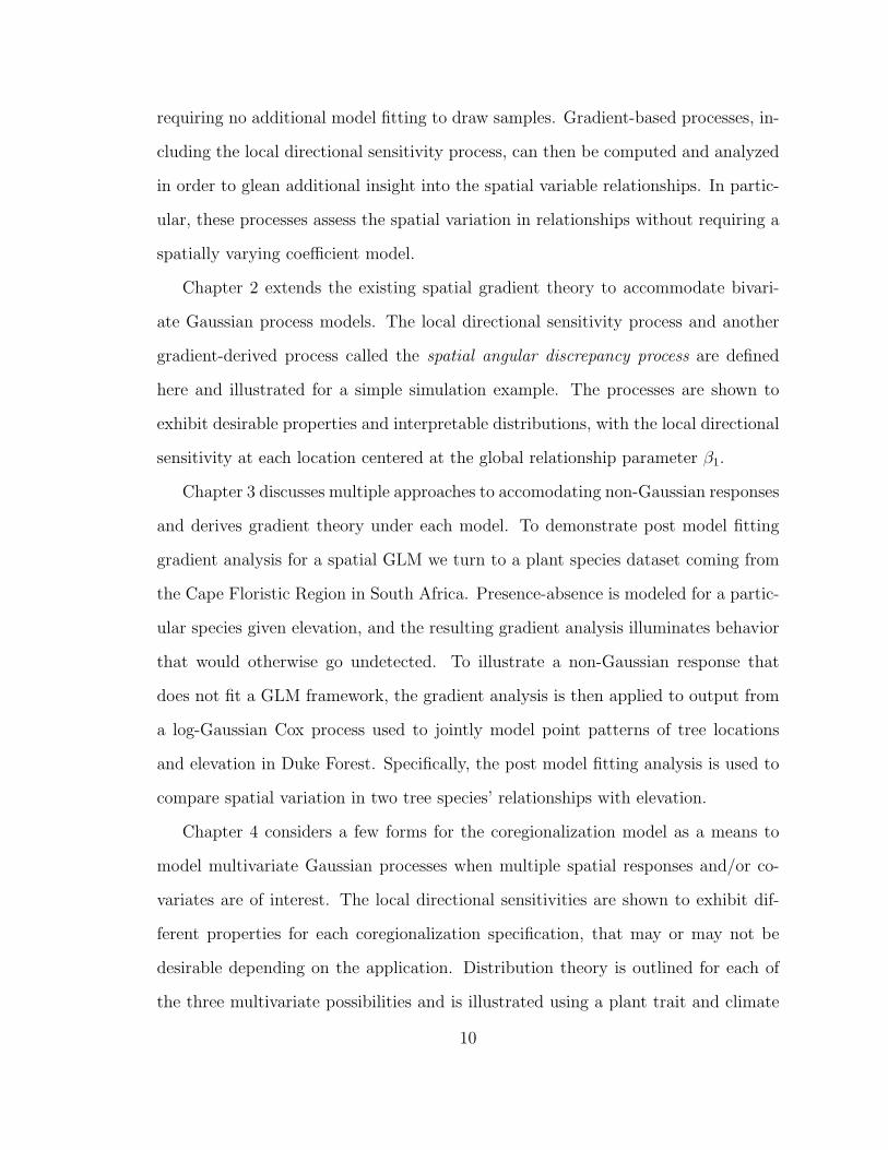
Chapter 2 extends the existing spatial gradient theory to accommodate bivari-

ate Gaussian process models. The local directional sensitivity process and another

gradient-derived process called the spatial angular discrepancy process are defined

here and illustrated for a simple simulation example. The processes are shown to

exhibit desirable properties and interpretable distributions, with the local directional

sensitivity at each location centered at the global relationship parameter β1.

Chapter 3 discusses multiple approaches to accomodating non-Gaussian responses

and derives gradient theory under each model. To demonstrate post model fitting

gradient analysis for a spatial GLM we turn to a plant species dataset coming from

the Cape Floristic Region in South Africa. Presence-absence is modeled for a partic-

ular species given elevation, and the resulting gradient analysis illuminates behavior

that would otherwise go undetected. To illustrate a non-Gaussian response that

does not fit a GLM framework, the gradient analysis is then applied to output from

a log-Gaussian Cox process used to jointly model point patterns of tree locations

and elevation in Duke Forest. Specifically, the post model fitting analysis is used to

compare spatial variation in two tree species’ relationships with elevation.

Chapter 4 considers a few forms for the coregionalization model as a means to

model multivariate Gaussian processes when multiple spatial responses and/or co-

variates are of interest. The local directional sensitivities are shown to exhibit dif-

ferent properties for each coregionalization specification, that may or may not be

desirable depending on the application. Distribution theory is outlined for each of

the three multivariate possibilities and is illustrated using a plant trait and climate

10

dataset from the Cape Floristic Region in South Africa. The dataset allows for anal-

ysis of a single response with multiple covariates as well as multiple responses with

a single covariate.

Finally, Chapter 5 discusses relevant theory for several additional spatial modeling

frameworks, including those outlined in subsection 1.1.2, further demonstrating the

versatility of post model fitting gradient analyses.

11

2

Bivariate Spatial Gradients

2.1 Introduction

Spatial regression models commonly assume a linear relationship and make inference

based on the coefficient assigned to the covariate. This coefficient describes the

expected change in response, given a unit change in covariate, providing a global

gradient. However, gradient behavior is expected to vary locally over the study

region, and such local, or second-order, behavior can be studied through spatial

gradient analysis.

Assuming a single response and single covariate of interest whose surfaces are

spatially smooth, then both can be treated as realizations from a stochastic process.

It may be believed that the rate of change of the covariate impacts the rate of

change of the response and that the relationship between the two surfaces may differ

across the domain. An example of this setting would consider species response to

climate. For instance, ecologists are increasingly interested in characterizing how

abundance and frequency of tree species relate to changes in climate (e.g. Canham

and Thomas, 2010; Thuiller et al., 2004; Thomas, 2010). Investigating the response of

12

plants to climate can be informative about the expected effects of climate change on

range distributions. For instance, we might want to learn how temperature gradients

affect abundance gradients. Another example might consider how, across a region,

phenological traits of a plant species, e.g., leaf size, leaf thickness, and leaf length-leaf

diameter ratio, respond to moisture, soil type, and topography.

The contribution of this chapter is to extend the existing gradient theory to ac-

commodate this sort of bivariate analysis by modeling the response and covariate

jointly. If we work in a hierarchical modeling framework and fit this joint model,

then corresponding gradients for the spatial surfaces can be sampled simultaneously

from the joint predictive distribution. Under a significant regression relationship it is

not sensible to investigate the gradient behavior of the surfaces marginally. Suitable

comparison between the gradient surfaces illustrates how sensitive the response sur-

face is to the covariate surface, as well as the strength of this relationship. The former

is accomplished through comparison between the directions of the maximum gradient

at a given location; the latter requires consideration of their directional derivatives

relative to one another. In particular, we introduce two new spatial processes, a

local directional sensitivity process and a spatial angular discrepancy process. These

inferential tools are developed and carried out on simulated data in the context of a

customary geostatistical model (Banerjee et al., 2004).

In section 2.2 the formal distribution theory for the spatial gradients is extended

to the multivariate case. Section 2.3 outlines the modeling framework for the simula-

tion example. This section also defines the two processes of interest, namely the local

directional sensitivity process and the spatial angular discrepancy process. Section

2.4 provides a simulated example with a multivariate Gaussian process setup as a

proof of concept. Finally, section 2.5 summarizes the contributions of the chapter.

13

2.2 Distribution Development

In this section we review the definitions and distributions presented in Banerjee et al.

(2003) and extend these ideas to consider a multivariate Gaussian process. We as-

sume locations s ∈ R2, 2-dimensional Euclidean space, however extension to a generic

d-dimensional setting is straightforward. The process is assumed, for convenience, to

be (weakly) stationary such that the covariance function, Cov(Y (s), Y (s′)), depends

only on the separation vector δ = s− s′. In fact, in our examples we adopt isotropic

covariance functions that depend only on the length of the separation vector, ||δ||.

Consider two surfaces (Y (s), X(s)) : s ∈ R2 drawn from a joint Gaussian

process specified such that X(s) has constant mean, say α0, and covariance function

G(δ). Given X(s), Y (s) has mean βX(s) and covariance function K(δ). Observed

at a set of locations Y = (Y (s1), . . . , Y (sn)), we write: Y|X ∼ N(βX, K(·)) with

X ∼ N(α0, G(·)). Considered jointly, we have:(YX

)∼ N

((α0β1α01

),

(K(·) + β2G(·) βG(·)

βG(·) G(·)

))

where G(·) and K(·) are matrices of the covariance functions with entry i, j evaluated

at δ = si − sj.

We follow the notation and theory in Banerjee et al. (2003). Assume mean

square differentiable processes Y (s) and X(s). That is, for Y (s), at s0 there exists

a vector ∇Y (s0) such that for any scalar h and any unit vector u, Y (s0 + hu) =

Y (s0) + huT∇Y (s0) + r(s0, hu) where r(s0, hu) → 0 in the L2 sense as h → 0.

Similarly, for X(s).

In particular, define the finite difference processes at scale h in direction u:

Yu,h(s) =Y (s + hu)− Y (s)

h

Xu,h(s) =X(s + hu)−X(s)

h

14

where u is a unit vector. Taking the limit as h tends to 0, Banerjee et al. (2003)

define the directional derivative processes in the direction u:

DuY (s) = limh→0

Yu,h(s) = u′∇Y (s)

DuX(s) = limh→0

Xu,h(s) = u′∇X(s)

where ∇X(s) = (De1X(s), De2X(s))′ is the vector of directional derivatives in the

orthonormal basis directions e1 = (1, 0) and e2 = (0, 1) for R2. We can study the

directional derivative processes for any u by working with the basis set ∇Y (s) and

∇X(s).

From Banerjee et al. (2003), we know that if Y (s) and X(s) are stationary

Gaussian processes, then the resulting marginal distributions involving the direc-

tional derivatives will be stationary Gaussian processes as well. Note, isotropy in

the Y (s) process does not induce isotropy in the DuY (s) process; only stationar-

ity will be inherited. Similar to the discussion in their paper, we know by lin-

earity that (Y (s), X(s), Yu,h(s), Xu,h(s))′ will be a stationary multivariate Gaussian

process. And then, by a standard limiting moment generating function argument,

(Y (s), X(s), DuY (s), DuX(s))′ will also be a stationary multivariate Gaussian pro-

cess.

To explicitly provide the joint distribution, we derive the cross covariance struc-

ture by examining pair-wise covariances between the response and covariate processes

and their directional derivatives. For notational convenience, write the marginal co-

variance function of Y (s) to be K(·) = K(·) + β2G(·). Assume the Y (s) and X(s)

processes are mean-zero, setting α0 = 0, since in practice the gradients are calculated

for the mean-zero residual process. If E(Y (s)) = 0, then E(DuY (s)) = 0, so the

joint processes will all be mean-zero. We calculate the covariances associated with

the directional derivatives by taking the limits of the covariances corresponding to

the analogous finite difference process.

15

The covariances for the response surface are derived in Banerjee et al. (2003):

Cov(Yu,h(s), Yu,h(s′)) =

2K(δ)− K(δ + hu)− K(δ − hu)

h2

Cov(DuY (s), DuY (s′)) = limh→0

Cov(Yu,h(s), Yu,h(s′)) = −u′ΩKu

Cov(Y (s), Yu,h(s′)) =

K(δ − hu)− K(δ)

h

Cov(Y (s), DuY (s′)) = limh→0

Cov(Y (s), Yu,h(s′)) = DuK(−δ)

and covariances for the covariate surface are analogous:

Cov(Xu,h(s), Xu,h(s′)) =

2G(δ)−G(δ + hu)−G(δ − hu)

h2

Cov(DuX(s), DuX(s′)) = limh→0

Cov(Xu,h(s), Xu,h(s′)) = −u′ΩGu

Cov(X(s), Xu,h(s′)) =

G(δ − hu)−G(δ)

h

Cov(X(s), DuX(s′)) = Cov(X(s), Xu,h(s′)) = DuG(−δ)

To fully describe the joint distribution we derive the covariances between response

and covariate surfaces similarly:

Cov(Y (s), Xu,h(s′)) =

βG(δ − hu)− βG(δ)

h

Cov(Y (s), DuX(s′)) = limh→0

Cov(Y (s), Xu,h(s′)) = βDuG(−δ)

16

Cov(X(s), Yu,h(s′)) =

βG(δ − hu)− βG(δ)

h

Cov(X(s), DuY (s′)) = limh→0

Cov(X(s), Yu,h(s′)) = βDuG(−δ)

Cov(Xu,h(s), Yu,h(s′) =

2βG(δ)− βG(δ + hu)− βG(δ − hu)

h2

Cov(DuX(s), DuY (s′)) = limh→0

Cov(Xu,h(s), Yu,h(s′) = −βu′ΩG(δ)u

where (ΩG(δ))ij = ∂2G(δ)/∂δi∂δj and DuG(δ) = limh→0(G(δ − hu)−G(δ))/h.

Relationships between the response surface, the covariate surface and their corre-

sponding directional derivative surfaces can be described through the 6-dimensional

multivariate stationary Gaussian process Z(s) = (Y (s), X(s),∇Y (s),∇X(s))′. Using

the covariances calculated above, the associated cross-covariance matrix for Z will

be:

VZ(δ) =

K(δ) βG(δ) −∇K(δ)′ −β∇G(δ)′

βG(δ) G(δ) −β∇G(δ)′ −∇G(δ)′

∇K(δ) β∇G(δ) −HK(δ) −βHG(δ)β∇G(δ) ∇G(δ) −βHG(δ) −HG(δ)

=

K(δ) + β2G(δ) βG(δ) −∇K(δ)′ − β2∇G(δ)′ −β∇G(δ)′

βG(δ) G(δ) −β∇G(δ)′ −∇G(δ)′

∇K(δ) + β2∇G(δ) β∇G(δ) −HK(δ)− β2HG(δ) −βHG(δ)β∇G(δ) ∇G(δ) −βHG(δ) −HG(δ)

where ∇K(δ) is a 2×1 gradient vector associated with K(δ), and HK(δ) is the 2×2

Hessian matrix associated with K(δ).

17

For δ = 0, we have a block diagonal local covariance matrix:

VZ(0) =

K(0) + β2G(0) βG(0) 0′ 0′

βG(0) G(0) 0′ 0′

0 0 −HK(0)− β2HG(0) −βHG(0)0 0 −βHG(0) −HG(0)

.

Thus, at a location s, the directional derivative surfaces will be correlated with one

another, but neither will be correlated with either of the data surfaces. Intuitively,

this makes sense since we would not expect the level of the surface at a location to

be correlated with the rate of change at that location. Of course, since (X(s), Y (s))′

is a bivariate Gaussian process, the correlation between the rates of changes is not

surprising.

The Matern covariance is adopted below. It depends on a smoothness parameter

ν which directly controls the mean square differentiability of process realizations

(Stein, 1999). This is convenient since, again, the Y (s) and X(s) processes must be

mean square differentiable for their associated directional derivative processes to be

well defined. If we let K(·) and G(·) be Matern with ν > 1 then they are once (but

not twice) mean square differentiable, and, if ν = 3/2, the covariance functions are

of the closed form σ2(1 + φ||δ||) exp(−φ||δ||). We denote the parameters of K(·) as

σ2y and φy, and the parameters of G(·) as σ2

x and φx.

Under the Matern covariance the components of the cross-covariance matrix will

be∇K(δ) = −σ2yφ

2y exp(−φy||δ||)δ, (HK(δ))ii = −σ2

yφ2y exp(−φy||δ||)(1−φyδ2

i /||δ||),

(HK(δ))ij = σ2yφ

3y exp(−φy||δ||)δiδj/||δ||, and similar for G(·). Then, we have for

δ = 0:

VZ(0) =

σ2y + β2σ2

x βσ2x 0′ 0′

βσ2x σ2

x 0′ 0′

0 0 (σ2yφ

2y + β2σ2

xφ2x)I2 (βσ2

xφ2x)I2

0 0 (βσ2xφ

2x)I2 (σ2

xφ2x)I2

(2.1)

where I2 is the 2× 2 identity matrix. As above, De1Y (s) and De1X(s) will be corre-

lated with one another, and similarly De2Y (s) and De2X(s) will be correlated with

18

one another, but all other pairings of the directional derivatives will be uncorrelated.

2.3 Model Fitting and Inference

2.3.1 Sampling Method

Following the modeling of the previous section, let K(δ) = σ2yρy(δ) and G(δ) =

σ2xρx(δ), where the ρx and ρy are valid two-dimensional correlation functions. We

work with the Matern class of covariance functions parameterized by φ and ν with

ν > 1.

Let θ = (α0, β0, β1, σ2x, σ

2y, φx, φy, νx, νy). For locations s1, . . . , sn, the overall like-

lihood can be written in terms of the conditional likelihoods

L(θ; Y,X) ∝ L(Y|θ,X)L(X|θ)

∝ (σ2xσ

2y)−n/2|Rx(φx, νx)|−1/2|Ry(φy, νy)|−1/2

× exp

− 1

2σ2x

(X− α01)′R−1x (φx, νx)(X− α01)

× exp

− 1

2σ2y

(Y − (β01 + β1X))′R−1y (φy, νy)(Y − (β01 + β1X))

where Y = (Y (s1), . . . , Y (sn))′, (Rx(φx, νx))ij = ρx(si−sj;φx, νx) and (Ry(φy, νy))ij =

ρy(si− sj;φy, νy). The likelihood could be equivalently written in its joint form, but

the conditional form is more conducive to interpreting and implementing the gradient

analysis.

We see that we have a low dimensional parametric model, with θ only 9 dimen-

sional. We utilize fairly non-informative priors for its components. For example,

vague normal priors on (α0, β0, β1), vague inverse Gamma priors on (σ2x, σ

2y), vague

Gamma priors on (φx, φy), and U(1, 2) priors on (νx, νy). The prior on ν follows the

suggestion of Stein (1999) and others who observe that distinguishing ν = 2 from

ν > 2 would be very difficult in practice. This model is straight forward to fit in its

19

conditional form, for example using the ‘spBayes’ package in R (Finley et al., 2007).

Thus, assume we now have posterior samples θ∗l , l = 1, . . . , L, from f(θ|Y,X).

Once we have posterior samples of the parameters, we draw samples of the

gradient vectors using composition since the posterior predictive distribution

f(∇Y ,∇X |Y,X) =∫f(∇Y ,∇X |Y,X,θ)f(θ|Y,X)dθ. The cross-covariance ma-

trix derived earlier allows us to immediately write the joint multivariate normal

distribution given θ, which can be evaluated at each sample θ∗l . Based on this joint

distribution, standard multivariate normal theory allows us to write down the desired

conditional distributions needed to draw from the predictive distribution.

For an unobserved location s0, obtaining draws of the gradient vectors is again

done via the predictive distribution. The cross covariance matrix derived enables

us to write the joint distribution, from which we can derive the conditional dis-

tribution f(∇Y (s0),∇X(s0)|Y,X,θ). If interest is also in the values of the Y (s)

and X(s) surfaces at the new location, we would derive the conditional distribution

f(Y (s0), X(s0),∇Y (s0),∇X(s0)|Y,X,θ), which is again straight forward given the

cross covariance matrix and allows joint prediction of the surfaces and their gradients

at the new location.

If we want Y (s) and X(s) to be adjusted based on some fixed covariates, then we

simply introduce such covariates into the mean functions of the model. We create a

spatial random effects model:

Y (s)|X(s) = β0 + β1X(s) + Ty(s)′γy + wy(s) + ε(s)

X(s) = α0 + Tx(s)′γx + wx(s)

where Ty(s) and Tx(s) are vectors of covariates used to explain the Y (s) and X(s)

surfaces respectively, with coefficients γy and γx; wy(s) and wx(s) are independent

mean-zero stationary Gaussian processes with parameters σ2x, σ

2y, φx, φy, νx, νy as be-

fore; and ε(s) is a Gaussian white-noise process with variance τ 2 intended to capture

20

measurement error or microscale variability in the response. The X(s) process is

assumed to be a fully spatial model (no nugget effect), such as might be used for

elevation, temperature, or pollutant level.

With θ now extended to θ = (α0, β0, β1,γx,γy, σ2x, σ

2y, φx, φy, νx, νy), the likeli-

hood for locations s1, . . . , sn above can be trivially revised. Prior selection for the

parameters will be similar to the previous example. Again, this model can be im-

plemented using ‘spBayes’, and draws of the gradients will rely on the posterior

predictive distribution, which can be calculated as before using the derived cross-

covariance matrix.

2.3.2 Local Directional Sensitivity Process

At a given location s there may additionally be interest in the ratio of directional

derivatives, DuY (s)/DuX(s), corresponding to the relative rates of change in the

two surfaces in direction u. This quantity is analogous to dy/dx in more standard

calculus applications as well as sensitivity functions studied in sensitivity analysis

(Tomovic and Vukobratovic, 1972). With this in mind, we refer to the resulting

spatial process as the local directional sensitivity process. The choice of u will depend

on the application being considered. For example, this direction may correspond to

latitudinal direction, an elevation direction, or to an environmental feature expected

to impact the response. Large values of this process would suggest that the change

in covariate surface has a high impact on the response surface.

The joint process defined in Section 2.2 can be equivalently represented as a

21

spatial random effects model (excluding nugget effects):

Y (s)|X(s) = β0 + β1X(s) + wy(s)

X(s) = α0 + wx(s)

wy(s) ∼ GP (0, K(δ))

wx(s) ∼ GP (0, G(δ))

where wy(s) and wx(s) are independent processes. With this notation we can write

the unconditional response surface and corresponding directional derivative process

as follows:

Y (s) = β0 + β1α0 + β1wx(s) + wy(s)

DuY (s) = β1Duwx(s) +Duwy(s)

The local directional sensitivity process can then be written

DuY (s)

DuX(s)=β1Duwx(s) +Duwy(s)

Duwx(s)= β1 +

Duwy(s)

Duwx(s)(2.2)

We see that the multiplicative parameter, β1, defining the overall relationship be-

tween the X(s) and Y (s) processes serves to center the local directional sensitivity

process.

As mentioned in Majumdar et al. 2006, if we consider Y (s) = β0 +β1X(s)+ ε(s),

then one could write β1 = dE(Y (s))/dX(s); i.e., β1 is describing the rate of change

in E(Y (s)) relative to changes in X(s). Again, at any location the local direc-

tional sensitivity will be centered at the global (non-directional) derivative ratio

dE(Y (s))/dX(s) plus some (directional) spatial noise. In this way, the local direc-

tional sensitivity process is describing the spatial variation in the relative rates of

change between X(s) and Y (s). This is analogous to modeling adopting spatially

varying coefficients, β(s), (Gelfand et al., 2003) but is arguably a simpler context

since the derivatives require no additional model fitting. In addition, consideration

22

of directional perspectives using this gradient approach allows for inference distinct

from what one can learn from a non-directional β(s) parameter.

By noting that Duwy(s)/Duwx(s) is a ratio of independent mean zero normal

random variables, at each location the directional spatial noise is a Cauchy ran-

dom variable with scale equal to the ratio of the respective standard deviations,

SD(Duwy(s))/SD(Duwx(s)). If u = (u1, u2), then

SD(Duwy(s)) =√u2

1(−HK(0)1,1) + u22(−HK(0)2,2)

If Y (s) is isotropic, then HK(0) = coI2 (Banerjee et al., 2003) and SD(Duwy(s)) =√u2

1 + u22

√−c0 =

√−c0. If K(·) and G(·) are Matern with ν = 3/2, then

SD(Duwi(s)) = σiφi, and the scale for the Cauchy distribution will be σyφy/σxφx.

When the respective standard deviations are equal, the scale will be 1 and the di-

rectional derivative ratio will have a standard Cauchy distribution.

In fact, the collection of directional derivative ratios form a well defined spatial

stochastic process which would naturally be called a spatial Cauchy process (see

Appendix A.1 for details). For any set of locations s1, . . . , sn the joint distribution is

well defined. For example, consider two locations s and s′, simplifying the notation

for clarity:

P (Duwy(s)

Duwx(s)< r1,

Duwy(s′)

Duwx(s′)< r2) = P (

n1

m1

< r1,n2

m2

< r2)

= P (n1 < r1m1, n2 < r2m2, m1 > 0, m2 > 0)

+ P (n1 < r1m1, n2 > r2m2, m1 > 0, m2 < 0)

+ P (n1 > r1m1, n2 < r2m2, m1 < 0, m2 > 0)

+ P (n1 > r1m1, n2 > r2m2, m1 < 0, m2 < 0)

In turn, each of these terms can be computed as an integral involving normal densi-

23

ties. For example, the first term can be written as follows:

P (n1 < r1m1, n2 < r2m2,m1 > 0,m2 > 0) =∫ ∞0

∫ ∞0

∫ r1m1

−∞

∫ r2m2

−∞fK(n1, n2)fG(m1, m2)dn2dn1dm2dm1 (2.3)

where fK(n1, n2) = fK(Duwy(s), Duwy(s′)) is the bivariate normal density for the

Duwy(s) Gaussian process with parent covariance function K(·) evaluated at s and

s′, and similar for fG(m1,m2). Recall that a univariate Cauchy distribution can be

defined as a scale mixture of normals (Andrews and Mallows, 1974). If we write

the corresponding cdf as F (r) =∫∞

0

∫ rm−∞ φ(n)φ(m)dndm, then the form in (2.3) is

evidently similar and can be regarded as a bivariate analogue. In this way, the spatial

Cauchy process is defined such that at any location the distribution is a univariate

Cauchy distribution and for any set of locations the distribution is a sum of integrals

of a similar form.

In the data analysis examples we consider a fixed direction u and draw samples of

the directional derivative ratio at each location across a region. Although we cannot

show mean square continuity for this surface, by imposing additional smoothness

conditions on the covariance functions for wy(s) and wx(s), we can argue that this

surface will be almost surely continuous using results from Kent (1989), following

the development in Banerjee and Gelfand (2003). We omit the details.

2.3.3 Spatial Angular Discrepancy Process

At any given location there may be interest not only in the magnitude of the gradients

in various directions, but also in the direction at which the maximum gradients are

achieved. Stronger alignment between the directions of maximum gradients would

suggest a stronger relationship between the response and covariate surfaces.

Consider the covariate process X(s). At location s the maximum gradient will

be achieved in the direction described by the unit vector u∗X = ∇X(s)/||∇X(s)||, and

24

the directional derivative in the direction of maximum gradient will be Du∗XX(s) =

||∇X(s)|| (Banerjee et al., 2003). We can similarly consider the direction of maxi-

mum gradient for the response surface which will occur for u∗Y = ∇Y (s)/||∇Y (s)||.

In applications, researchers may be interested in the behavior of the response sur-

face, or its relative rate of change, in the direction u∗X . That is, there may be

interest in Du∗XY (s) = ∇X(s)′∇Y (s)/||∇X(s)|| as well as Du∗X

Y (s)/Du∗XX(s) =

(∇X(s)′∇Y (s))/(∇X(s)′∇X(s)).

At a location s the magnitude of the maximum gradient, ||∇X(s)||, will be the

square root of a sum of squared independent normal random variables; as such, this

quantity will have a Chi distribution with d = 2 degrees of freedom, possibly scaled

by some factor. If the process is isotropic, then ||∇X(s)|| will have a Chi distribution

with d = 2 degrees of freedom scaled by SD(De1X(s)) = SD(De2X(s)). For the

Matern covariance (ν = 3/2) structure this scaling factor will be equal to σxφx.

The unit vector describing the direction of max gradient for the covariate surface

can equivalently be described by an angle θX(s) such that

tan(θX(s)) = D(0,1)X(s)/D(1,0)X(s), and similarly for the response surface. The

angle θ can take values from −π to π, so inversion of tan must be done with care.

Since tan has a period of only π, the inverse function is typically taken to be arctan∗.

(arctan∗(S/C) is arctan(S/C) if C > 0, S ≥ 0; π/2 if C = 0, S > 0; arctan(S/C)+π

if C < 0; arctan(S/C) + 2π if C ≥ 0, S < 0; and undefined if C = 0, S = 0

(Jammalamadaka and Sengupta, 2001).)

As smooth functions of a well defined spatial process, the directions of maximum

gradient (θX(s), θY (s)) define a bivariate projected Gaussian process, analogous to

the univariate projected Gaussian processes described in Wang (2013). Marginally

θX(s) and θY (s) will each be a projected Gaussian process (Wang, 2013). Assuming

the Matern (ν = 3/2) covariance structure we can derive the joint distribution of the

25

two angles at a given location s:

f(θX(s), θY (s)) =

C

(B +

√2πA(s)

(ac−A2(s))3/2L(0, 0,

√A2(s)ac

) + φ(0)ac

), A(s) > 0

C

(B +

√2πA(s)

(ac−A2(s))3/2

(0.5− L(0, 0,

√A2(s)ac

)

)+ φ(0)

ac

), A(s) < 0

where C = 1

a(2π)3/2√|Σ|

, B = A2(s)φ(0)

ac(ac−A2(s)), |Σ| = (σ2

xφ2x)

2(σ2yφ

2y)

2, a = 1/(σ2yφ

2y), c =

(σ2yφ

2y + β2φ2

xσ2x)/(σ

2xφ

2x), A(s) =

√aβ cos(θX(s) − θY (s)), and L(0, 0, ρ) is the zero

mean bivariate normal cdf with correlation ρ and standard deviations equal to 1

evaluated at (0, 0). A brief derivation is provided in Appendix A.2. In addition, it

is straightforward to show that at each location s the angles, θX(s) and θY (s), will

marginally be uniform on (−π, π).

The above bivariate density is plotted in Figure 2.1 for β = (±0.05,±0.5,±1)′,

holding all other parameters constant: σy = 1 = σx and φy = 1.05 = φx. When β > 0

the mass is concentrated around (θX , θY ) pairs that are equal; when β < 0 the mass

is concentrated around pairs where θX = θY − π. When β = ±0.05 the relationship

between X(s) and Y (s) is weak, and the density is roughly uniform over all angle

pairs. As the magnitude of β increases, the mass becomes increasingly concentrated

around these respective values.

To compare the directions of maximum gradient calculated from the posterior

distribution, we compute a “discrepancy” for θX(s) and θY (s). Define: disc(s) =

1 − cos(θX(s) − θY (s)). As a smooth function of a spatial process, this discrepancy

is a well defined spatial process which we refer to as the spatial angular discrepancy

process. When the maximum gradients occur in identical directions this process will

have a value of zero, when they occur in opposite directions the process will have a

value of two. In our analyses we consider the process across a region, plotting the

posterior median surface.

In some areas the X(s) or Y (s) surface may be quite flat and there will be no

26

−3 −2 −1 0 1 2 3

−3

−2

−1

01

23

β= 0.05

θx

θy

−3 −2 −1 0 1 2 3

−3

−2

−1

01

23

β= 0.5

θx

θy

−3 −2 −1 0 1 2 3

−3

−2

−1

01

23

β= 1

θx

θy

−3 −2 −1 0 1 2 3

−3

−2

−1

01

23

β= −0.05

θx

θy

−3 −2 −1 0 1 2 3

−3

−2

−1

01

23

β= −0.5

θx

θy

−3 −2 −1 0 1 2 3

−3

−2

−1

01

23

β= −1

θx

θy

0.02

0.04

0.06

0.08

Figure 2.1: Bivariate density for (θX(s), θY (s)) at a fixed s for varying values of β.All other parameters are set to the values used for simulation in Section 2.4.

direction with a gradient magnitude substantially larger than in the other directions.

In these areas a large angular discrepancy may not be as meaningful as it would be

in areas with larger gradient magnitudes. For this reason it is useful to examine

these plots in tandem with plots of the local directional sensitivity process described

in Section 2.3.2.

2.4 Simulation Example

We consider a simulation example to explore the behavior of gradient quantities in a

controlled setting. From the foregoing development, in the context of spatial gradient

analysis the quantities of interest will be directional derivatives. These derivatives

are unobservable even in a simulation study with known parameters. Thus, assessing

inference performance with regard to these quantities requires some novelty.

Recall that the gradient processes describe the shape and behavior of spatial sur-

27

faces. With a simulated dataset, we are able to draw a realization of the Gaussian

process over a larger number of locations, allowing for fairly detailed understanding

of the spatial surfaces. To avoid any unfair advantage that might come from the

increased sample size, we use only a subset of the locations to fit the model and

reserve the full set of locations for assessing the quality of our inference. Contour

lines highlighting the shape of the surface are interpolated using the full set of loca-

tions. Conclusions made using gradients are then compared to those suggested by

the contour lines to examine performance.

2.4.1 Data and Model

We simulate X(s) a realization from a mean zero Gaussian process on [0, 10]× [0, 10],

and Y (s)|X(s) a realization from a Gaussian process with mean βX(s). We use

Matern covariance functions setting ν = 3/2 in order to capitalize on the resultant

closed form. We simulate the Gaussian processes assuming Matern covariance func-

tions with parameters φx = 1.05 = φy, σ2x = 1 = σ2

y, β0 = 0 = α0, and β1 = 0.5.

We draw a larger realization at 2000 locations, to allow for finer knowledge of the

underlying surface, from which we consider a subset of 200 locations to be our “ob-

servations”.

Treating (Y (s), X(s))′ as a multivariate Gaussian process, we fit a coregionaliza-

tion model using the conditional parameterization, as described in Section 2.2. The

model is fitted using the ‘spbayes’ package in R by first fitting parameters for X(s),

then fitting parameters for Y (s)|X(s). We obtain 2000 samples after a burn-in of 500

iterations and a thinning of every fifth iterate. We assume ν = 3/2. Priors for the

remaining parameters are: α0 ∼ N(0, 100), β0 ∼ N(0, 100), β1 ∼ N(0, 100), φx, φy ∼

U(0.5, 10), σ2x, σ

2y ∼ IG(2, 0.1) where α0 = E(X(s)) and β0+β1X(s) = E(Y (s)|X(s)).

Summaries of the posterior parameter samples are provided in Table 2.4.1.

We consider a region centered at the location s∗ = (7.5, 6.5). The X(s) and Y (s)

28

Table 2.1: Parameter estimates for the [Y (s)|X(s)][X(s)] model.

Parameter 0.025 Mean 0.975 Truthα0 -0.7126 -0.0614 0.6214 0β0 0.2726 0.8179 1.3867 0β1 0.4685 0.5943 0.7202 0.5σ2x 0.6725 1.0692 1.7390 1φx 0.8242 1.0230 1.2124 1.05σ2y 0.4911 0.8057 1.3341 1φy 0.8572 1.0718 1.3116 1.05

values at this location are provided in Figure 2.2. (The full processes were realized

on [0, 10]× [0, 10], but we only show a subregion here.) The interpolated surface and

contour lines are produced using the full 2000 locations, while the circles indicate

the subset of 200 locations used to predict the gradient.

6 7 8 9

56

78

−1.5

−1 −0.5

0.5

1

1

6 7 8 9

56

78

−0.5

0.5

1.5

1.5

2

2.5

3

−3

−2

−1

0

1

2

3

Figure 2.2: X(s) (left) and Y (s) (right) subregions around s∗, where we estimatethe gradient.

2.4.2 Local Directional Sensitivity Process

We are interested in the behavior of DuY (s)/DuX(s). We consider u = (1, 0) and

u = (0, 1). Since D−uY (s) = −DuY (s) (Banerjee et al., 2003), any discussion of

the behavior in u direction implies the opposite behavior is occurring in the opposite

direction. When applied to the ratios, this means that the local directional sensitivity

process will be equal for u and −u.

29

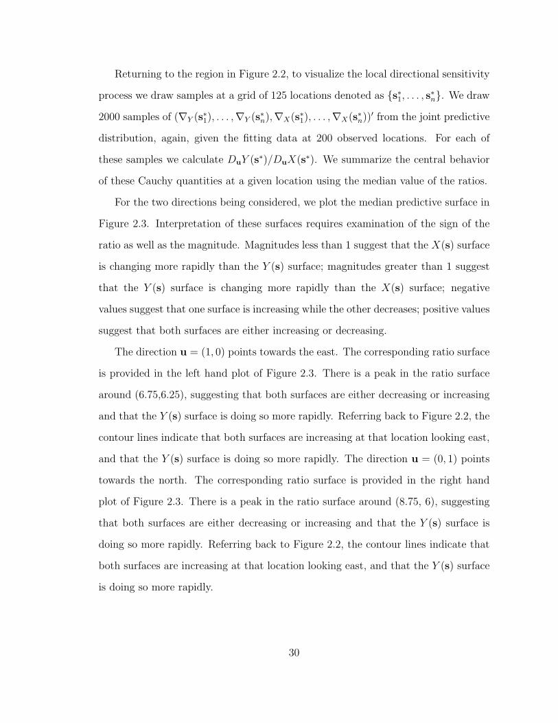
Returning to the region in Figure 2.2, to visualize the local directional sensitivity

process we draw samples at a grid of 125 locations denoted as s∗1, . . . , s∗n. We draw

2000 samples of (∇Y (s∗1), . . . ,∇Y (s∗n),∇X(s∗1), . . . ,∇X(s∗n))′ from the joint predictive

distribution, again, given the fitting data at 200 observed locations. For each of

these samples we calculate DuY (s∗)/DuX(s∗). We summarize the central behavior

of these Cauchy quantities at a given location using the median value of the ratios.

For the two directions being considered, we plot the median predictive surface in

Figure 2.3. Interpretation of these surfaces requires examination of the sign of the

ratio as well as the magnitude. Magnitudes less than 1 suggest that the X(s) surface

is changing more rapidly than the Y (s) surface; magnitudes greater than 1 suggest

that the Y (s) surface is changing more rapidly than the X(s) surface; negative

values suggest that one surface is increasing while the other decreases; positive values

suggest that both surfaces are either increasing or decreasing.

The direction u = (1, 0) points towards the east. The corresponding ratio surface

is provided in the left hand plot of Figure 2.3. There is a peak in the ratio surface

around (6.75,6.25), suggesting that both surfaces are either decreasing or increasing

and that the Y (s) surface is doing so more rapidly. Referring back to Figure 2.2, the

contour lines indicate that both surfaces are increasing at that location looking east,

and that the Y (s) surface is doing so more rapidly. The direction u = (0, 1) points

towards the north. The corresponding ratio surface is provided in the right hand

plot of Figure 2.3. There is a peak in the ratio surface around (8.75, 6), suggesting

that both surfaces are either decreasing or increasing and that the Y (s) surface is

doing so more rapidly. Referring back to Figure 2.2, the contour lines indicate that

both surfaces are increasing at that location looking east, and that the Y (s) surface

is doing so more rapidly.

30

6 7 8 9

56

78

0

0

0

0

0.5

0.5

0.5

1

1

1

1

1

1

1

1.5

1.5

1.5

1.5

2

2

2

2

2.5

3

6 7 8 9

56

78

−1

0

0

0

0.5

0.5

0.5

1

1

1

1

1

1

1

1.5

1.5

1.5

2

2

2

2.5 3

−2

−1

0

1

2

Figure 2.3: Posterior median of DuY (s)/DuX(s) in the directions u = (1, 0) (left)and u = (0, 1) (right).

2.4.3 Spatial Angular Discrepancy Process

Consider again the region in Figure 2.2 and the grid of 125 locations denoted as

s∗1, . . . , s∗n. Sampling gradients from the joint predictive distribution for

(∇X(s∗i ),∇Y (s∗i ))′, we calculate the direction of maximum gradient as

∇X(s∗i )/||∇X(s∗i )|| and ∇Y (s∗i )/||∇Y (s∗i )|| for each sample gradient at each location

in the figure. Denote these angles (in radians) as θX(s∗i ) and θY (s∗i ) respectively.

We compute the discrepancy between these angles at each location as in Section

2.3.3 and provide the posterior median values in Figure 2.4. Most of the region

has an associated discrepancy of 0, suggesting that both X(s) and Y (s) are typically

increasing most rapidly in the same direction. However, there are a few small regions

where the discrepancy peaks towards a value of 2, locations where the X(s) and Y (s)

surfaces are increasing in nearly opposite directions.

2.5 Summary

We have extended previous theory on gradient analysis to allow for consideration of

a bivariate process where one variable is treated as a response to the other variable.

Consideration of the associated directional derivatives can be done jointly and results

31

6 7 8 9

56

78

0.0

0.5

1.0

1.5

2.0

0.2

0.2

0.2

0.2

0.2

0.2

0.4

0.4

0.4

0.4

0.4

0.6

0.6

0.6

0.6

0.6

0.6

0.6

0.8

0.8

0.8

0.8

0.8 0.8

0.8

1

1

1

1

1

1.2

1.2

1.4

1.6

1.8

1.8

Figure 2.4: Posterior median disc(s).

in a multivariate Gaussian process directly derivable from the model for the parent

process. The models for the parent process are fit in a Bayesian framework and

utilizing the posterior draws of the process parameters, all gradient analysis occurs

post model fitting.

Using the directional derivatives, we proposed two derived processes that are use-

ful for learning about the relationship between the response and covariate processes.

The first is the local directional sensitivity process. This process captures local vari-

ation in the relationship between the two variables and provides deeper insight into

their relative behavior. The second is the spatial angular discrepancy process, cap-

turing the discrepancy between the directions in which the process surfaces are most

rapidly increasing. Spatial plots of this discrepancy surface highlight regions of the

domain where the two processes behave most similarly and most differently.

The current theory provides opportunity for several extensions. Many ecological

data sets are observed at multiple time points, in part to see if the relationships

between the variables of interest are changing over time. With this in mind, future

work on gradient analyses may involve the incorporation of temporal effects. Ecolog-

ical data sets also tend to have multiple responses and multiple covariates, any or all

of which may have relationships that could be better highlighted through a gradient

32

analysis under a joint model. Finally, for many applications it will be important

to consider novel non-Gaussian responses modeled through latent Gaussian process

models.

33

3

Gradient Analysis for Non-Gaussian Responses

3.1 Introduction

While the methodology outlined in the previous chapter can readily accommodate

spatial data with a continuous response and covariate, it is common to have data that

naturally requires a non-Gaussian first stage for the model. Examples include binary

or zero-inflated data, but there are countless others. Appropriate spatial models for

these non-Gaussian responses include the class of spatial generalized linear models

(GLMs), as well as others that similarly rely on a transformation of a latent Gaussian

process. Computation of the directional derivative processes associated with these

non-Gaussian models is made possible through the spatial gradient chain rule, defined

in this chapter.

As a more basic spatial GLM example we use a dataset coming from a subregion

of the Cape Floristic Region (CFR) in South Africa to present a spatial GLM gradient

analysis with a binomial first stage. The analysis focuses on the spatial presence-

absence behavior of a Protea species in relation to elevation. The relationship is

explored at a regional level through examination of the spatial GLM parameters and

34

is explored at a more local level using the local directional sensitivity process and

spatial angular discrepancy process.

Next, we consider a more novel non-Gaussian response using point pattern data

from the Duke Forest. Conditional on elevation, point patterns for two tree species

are each modeled as a log-Gaussian Cox process, with elevation modeled as a spa-

tially varying intercept. The local directional sensitivity process and spatial angular

discrepancy process provide inference regarding the relationship between point pat-

tern intensity and elevation. One species illustrates a gradient analysis in the context

of a non-significant relationship with elevation, and the other illustrates a gradient

analysis in the context of a significant relationship with elevation.

The format of this chapter is as follows. The spatial gradient chain rule is outlined

in Section 3.2. In Section 3.3 we discuss procedures for implementing the gradient

analysis within a few spatial GLM frameworks. In Section 3.4 we detail the CFR data

used for analysis, outline the binomial model and derive associated gradient theory.

Results of the model fitting and gradient analyses are discussed with interpretations

in the context of the binomial model. Section 3.5 provides the analysis of point

pattern data from Duke Forest, illustrating gradient analysis for a log-Gaussian Cox

process and comparing gradient analyses across significant and non-significant spatial

regressions. Finally, Section 3.6 summarizes the results and contributions of the

chapter.

3.2 Extensions to Non-Gaussian Data Models Using the Chain Rule

For data where the response variable is inherently non-Gaussian, spatial dependence

is often captured through the use of a latent Gaussian surface. While the gradi-

ent analysis associated with these models will correspond to the latent Gaussian

process, and not to the response of interest, differentiable transformations will al-

low for inference on the non-Gaussian response surface. Recall the spatial gradi-

35

ent chain rule presented in Majumdar et al. (2006): for h(·) differentiable on R1

and W (s) = h(V (s)), the directional derivative DuW (s) exists and is given by

DuW (s) = Duh(V (s)) = h′(V (s))DuV (s). Here V (s) is the latent Gaussian sur-

face and the function h(·) describes its relationship to the non-Gaussian response.

For example, in the case of binary data h−1(·) may be the link function relating the

presence probability surface to a latent Gaussian process. Although the probability

surface is non-Gaussian, the spatial gradient chain rule allows for consideration of its

directional derivatives by examining the derivative of the inverse link function and

the directional derivative for the latent Gaussian processes. These ideas are further

detailed in the following examples.

3.3 Spatial Generalized Linear Models

A GLM replaces a model’s typical Gaussian first stage with another member of the

exponential family. The responses Y (s) are assumed to be conditionally independent

given the parameters, with distribution

f(Y (s)|β, γ) = h(Y (s), γ) exp(γ(Y (s)η(s)− ψ(η(s))))

g(η(s)) = X(s)β (3.1)

where g is a link function and γ is a dispersion parameter. These GLMs can be

modified to allow for spatial dependence through the introduction of a zero-mean

latent Gaussian process, commonly in the second stage of the hierarchical model.

E.g., the expression in (3.1) above can be modified such that g(η(s)) = X(s)β+wz(s)

where the spatial random effects wz(s) are realizations from a zero-mean Gaussian

process. The latent process induces marginal spatial dependence in the response

by encouraging the means of spatial variables at proximate locations to be similar

(Banerjee et al., 2004).

The use of latent Gaussian processes when building spatial GLMs allows for

36

straight forward application of the developed spatial process gradient methodology

for post model fitting analysis. Provided that the inverse link function g−1(·) is

differentiable, we can apply the spatial gradient chain rule to learn about the di-

rectional derivative processes for the mean function using the directional derivatives

associated with the latent Gaussian process (Majumdar et al., 2006). Implementing

such gradient analyses can be imagined for several spatial GLM frameworks, a few

of which are outlined here. As before, we will assume that the covariate variable can

additionally be assumed to follow a Gaussian process model.

The inference gained through post model fitting gradient analysis will have a

slightly different nature for the spatial GLMs than for the standard spatial linear

models. For a spatial linear model, say Y (s) = β0+β1X(s)+wy(s), we can investigate

the local rate of change for the response Y (s) at any location s and in any direction u

through the directional derivative DuY (s). However, for spatial GLMs the response

is typically non-continuous and a local rate of change is not meaningful. Taking

binary data as an example, the responses will always be either 1 or 0 and there will

never be a continuous change between responses. Instead we will consider the rates

of change of a latent mean surface η(s) = g−1(X(s)β), connected to the covariates

through a link function. Unlike the non-continuous response surface, this latent mean

surface will have a well defined directional derivative process which will inform on

its rates of change.

Understanding the relationship between the latent mean surface and the covariate

will be key to understanding the relationship with the response surface, though the

precise interpretation will differ depending on the mean function η (e.g., probabilities

vs. mean counts). The standard setup of the GLM allows for inference on this

relationship at a global scale through the coefficient on the covariate in the linear

form, β1. We can further investigate variations in magnitude and strength of this

relationship through the directional derivative processes. Examination of the local

37

directional sensitivity process can highlight local variation in the relationship both in

terms of sign and magnitude along different directional perspectives by comparing the

relative rates of change at each location in a given direction. In addition, the spatial

angular discrepancy process will inform on the spatial variation in the strength of the

relationship by comparing the directions of maximum gradient; a value of 0 suggests a

strong positive relationship while a value of 2 suggests a strong negative relationship.

This process is indicative of relationship strength since a pair of surfaces that are

most rapidly increasing in the same or opposite direction throughout the region

can be considered to have a stronger relationship than surfaces whose directions of

maximum gradient are less consistent with one another.

There are two common frameworks for constructing a spatial GLM, and the

choice of framework will be shown to impact the directional rates of change. The

first framework incorporates a latent Gaussian process as a spatial random effect in

the GLM’s linear second stage. The second framework defines the response variable

based on thresholding a latent Gaussian process. Both frameworks ultimately relate

the mean surface to the covariates through a link function, but not surprisingly

the different constructions lead to slightly different models and different gradient

processes as a result.

For each of the spatial GLM examples we will assume the latent Gaussian process

Z(s) is centered at a linear function of a spatial covariate X(s) which can be jointly

modeled using a Gaussian process. I.e., in each model we assume the following

relationship between Z(s) and X(s):

Z(s)|X(s) = β0 + β1X(s) + wz(s)

X(s) = α0 + wx(s)

wz(s) ∼ GP (0, ρz)

wx(s) ∼ GP (0, ρx)

38

where wz(s) and wx(s) are zero-mean spatial random effects surfaces.

To illustrate the first framework using spatial random effects consider binary

and count data, two common non-Gaussian responses. For binary data either a

spatial probit or logistic regression will typically be used where the observed presence

or absence, Y (s), is driven by the mean function η(s) = P (s) = P (Y (s) = 1).

This latent probability surface relates to a Gaussian process Z(s) through a link

function, either Φ−1(P (s)) = Z(s) for the probit regression or logit(P (s)) = Z(s)

for the logistic regression. Similarly, for count data one would use a spatial Poisson

regression where the observed counts follow a Poisson distribution with mean η(s) =

λ(s). A link function is again used to relate the mean surface to a latent Gaussian

process, log(λ(s)) = Z(s).

The relevant local directional sensitivity process will relate the rate of change in

the probability surface (for binary regression) or the mean surface (for Poisson re-

gression) to the rate of change in the covariate surface. Through the spatial gradient

chain rule these ratios can be expressed as simple functions of the independent Gaus-

sian processes. For example, for the probit model the local directional sensitivity will

be

DuP (s)

DuX(s)=DuΦ(Z(s))

DuX(s)

=φ(Z(s))DuZ(s)

DuX(s)

= φ(Z(s))(β1 +Duwz(s)

Duwx(s))

at any location s and for any direction u. I.e., the sensitivity for the latent prob-

ability surface can be written as the sensitivity for the latent Gaussian process,

DuZ(s)/DuX(s), weighted by φ(Z(s)), the normal pdf for that surface at the loca-

39

tion s. For Poisson regression the sensitivity will be

Duλ(s)

DuX(s)=Du exp(Z(s))

DuX(s)

=exp(Z(s))DuZ(s)

DuX(s)

= exp(Z(s))(β1 +Duwz(s)

Duwx(s))

at any location s and for any direction u. In this case, the sensitivity for the latent

Gaussian process, DuZ(s)/DuX(s), is weighted by exp(Z(s)).

The second spatial GLM framework involves thresholding latent Gaussian pro-

cesses. Bayesian modeling of non-Gaussian responses by thresholding latent nor-

mal random variables was originally proposed by Albert and Chib (1993), including

guidelines for both binary and multi-category data. These ideas have been extended

to accommodate spatially correlated data through the use of latent Gaussian pro-

cesses in place of the independent normal random variables (Heagerty and Lele, 1998;

Berrett and Calder, 2012). The mean function for the Gaussian process is assumed

to be a regression on covariates, and as before the spatial dependence in the latent

process encourages proximate locations to have similar presence probabilities.

For binary data the regression can be written

Y (s) =

1, if Z(s) > 0

0, if Z(s) < 0(3.2)

Z(s) ∼ GP (X(s)β, ρz(1, φz))

where the probability of presence at any location s can be written

P (s) = P (Y (s) = 1)

= Φ(X(s)β)

with Φ(·) denoting the standard normal cdf and ρz(·) a spatial correlation function

for the Gaussian process with the variance component set to 1 for identifiability.

40

To accommodate ordered multinomial data additional thresholds can be incor-

porated into the model in (3.2) such that each response category corresponds to a

specific range of values for the latent variable (Albert and Chib, 1993). To induce

spatial dependence, this model is again built using a Gaussian process specification.

For a multinomial response Y (s) ∈ 1, 2, 3 we have

Y (s) =

2, if a1 < Z(s) < a2

1, if a0 < Z(s) < a1

0, if a−1 < Z(s) < a0

(3.3)

Z(s) ∼ GP (X(s)β, ρz(1, φz))

where a2 = ∞ and a−1 = −∞. The probability that category i will be observed at

location s can be written

Pi(s) = P (Y (s) = i)

= Φ(ai −X(s)β)− Φ(ai−1 −X(s)β)

A similar model can be used to incorporate a point mass at zero, letting the

response equal zero if the latent Gaussian process is negative and equal to the latent

process otherwise:

Y (s) =

Z(s), if Z(s) > 0

0, if Z(s) < 0(3.4)

Z(s) ∼ GP (X(s)β, ρz(1, φz))

where the probability of a zero response is

P0(s) = P (Y (s) = 0)

= 1− Φ(X(s)β) = Φ(−X(s)β)

The gradient analyses for these models consider the rate of change of the asso-

ciated probability surface. Assuming a joint Gaussian process model for the latent

41

Z(s) process and the covariate X(s) process(es), the relationship between the prob-

ability surface and X(s) involves a differentiable function and the spatial gradient

chain rule can be applied in the usual way. For each of the above examples let the

mean function be

X(s)β = β0 + β1X(s)

X(s) = α0 + wx(s)

wx(s) ∼ GP (0, ρx(σ2x, φx))

Then, applying the spatial gradient chain rule, we can compute the directional deriva-

tives associated with each of the probability functions

DuP (s) = φ(β0 + β1X(s))β1Duwx(s)

DuPi(s) = (φ(ai−1 − β0 − β1X(s))− φ(ai − β0 − β1X(s)))β1Duwx(s)

DuP0(s) = −φ(−β0 − β1X(s))β1Duwx(s)

for the binary, multinomial and point mass at zero models respectively. Unlike

the spatial random effects framework, the directional derivative processes for these

probability surfaces do not involve the directional derivative for the latent Gaussian

process Z(s).

To compare the relative rates of change between the probability surface and the

covariate surface the local directional sensitivity processes can be computed for each

model

DuP (s)

DuX(s)= φ(β0 + β1X(s))β1 (3.5)

DuPi(s)

DuX(s)= (φ(ai−1 − β0 − β1X(s))− φ(ai − β0 − β1X(s)))β1

DuP0(s)

DuX(s)= −φ(−β0 − β1X(s))β1

These local directional sensitivities do not involve the directional derivative processes

for the X(s) process nor the latent Z(s) process, instead depending only on the

42

thresholds, β parameters, and the covariate process X(s). Additionally, these forms

reveal a lack of directional dependence. The directional derivative at location s will

be the same for any choice of u.

Alternatively, following the form for the spatial probit model described by Hea-

gerty and Lele (1998), one can include a nugget effect so that the latent Z(s) =

X(s)β + wz(s) + ε(s) where wz(s) ∼ GP (0, ρz(σ2z , φz)) and ε(s) ∼ N(0, 1− σ2

z). For

the binary model, the resulting probability surface, associated directional derivative

and local directional sensitivity will be

P (s) = Φ(X(s)β + wz(s)√

1− σ2z

)

DuP (s) = φ(X(s)β + wz(s)√

1− σ2z

)(β1√

1− σ2z

Duwx(s) +1√

1− σ2z

Duwz(s))

DuP (s)

DuX(s)= φ(

X(s)β + wz(s)√1− σ2

z

)(β1√

1− σ2z

+1√

1− σ2z

Duwz(s)

Duwx(s))

Unlike the local directional sensitivities in (3.5), when the nugget is included in the

model the local directional sensitivity will depend on the relative rates of change of

the latent Gaussian processes for Z(s) and X(s).

For each spatial GLM the spatial angular discrepancy process informs on the

strength of the relationship between the mean surface and the covariate. It can be

computed as disc(s) = 1 − cos(θX(s) − θη(s)), where θX(s) and θη(s) are the direc-

tion of maximum gradient for the covariate surface and mean surface respectively.

These directions are easily computed as the angles associated with the unit vec-

tors ∇X(s)/||∇X(s)|| and ∇η(s)/||∇η(s)|| shown to define the direction of maximum

gradient by Banerjee et al. (2003).

43

3.4 South Africa Protea, Elevation Analysis

3.4.1 Cape Floristic Region Data

To demonstrate a binomial spatial GLM we consider a subset of the Protea Atlas data

set (Rebelo, 2002) with elevation data from the South African Atlas of Hydrology

and Climatology (Schultze, 1997) previously prepared for analysis by Gelfand et al.

(2006) to examine species distributions and biodiversity. The data come from the

Cape Floristic Region (CFR) in South Africa, the smallest of the world’s six floral

kingdoms (Takhtajan et al., 1986) and a well known biodiversity hotspot. The iconic

flowering plant family in this region is the Protea family (Proteaceae), displaying high

rates of endemism with 330 of the roughly 400 African species being 99% restricted

to the CFR (Gelfand et al., 2006).

The subregion being considered is roughly rectangular with a total area of 4,456

km2 and overlaps the Kogelberg Biosphere Reserve and surroundings. The data

were originally collected at geo-referenced plots throughout the region, recording the

presence or absence of protea species within each plot. Here, the data are provided

in the form of 1554 minute by minute areal units (approximately 1.85 km × 1.55

km), aggregating information from all of the plots within each areal unit. For our

purposes areal units that did not contain any plots provide no information and were

removed from the data. This left a total of 962 areal units, with centroids plotted in

Figure 3.1.

We focus on the protea species spear-leaved conebush (Leucadendron spissi-

folium), present in 33.7% of the areal units. For each areal unit the data provide a

number of plots N(s) > 0 visited within the cell, the number of plots Y (s) where

presence was observed, and an elevation X(s). Interpolated surfaces for the observed

presence rates Y (s)/N(s) and elevation X(s) are provided in Figure 3.1.

44

300 310 320 330 340

6200

6220

6240

6260

6280

6300

Easting

Nor

thin

g

300 310 320 330 340

6200

6220

6240

6260

6280

6300

0.0

0.2

0.4

0.6

0.8

1.0

300 310 320 330 340

6200

6220

6240

6260

6280

6300

500

1000

1500

Figure 3.1: Centroids of observed areal units (left), interpolated Y (s)/N(s) surface(center) and interpolated X(s) surface (right).

3.4.2 Binomial Model and Spatial Gradients

These data are modeled using a spatial binomial regression with a logit link func-

tion, a natural extension of the binary models discussed earlier. For each areal unit

centered at location s we observe a number of samples N(s), with a total of Y (s)

presences observed for the given species, assumed to follow a binomial first stage

model [Y (s)|X(s)]. To define our joint spatial model we implement a spatially vary-

ing intercept model for the elevation covariate X(s).

For the areal unit centered at s, let P (s) be the presence probability and Z(s) be

a latent Gaussian process driving the presence probabilities. Then our model is

Y (s)|N(s), P (s) ∼ Bin(N(s), P (s))

log(P (s)

1− P (s)) = Z(s)

Z(s)|X(s) = β0 + β1X(s) + wz(s)

X(s) = α0 + wx(s)

wz(s) ∼ GP (0, ρz(φz, σ2z))

wx(s) ∼ GP (0, ρx(φx, σ2x))

45

where wz(s) and wx(s) represent independent spatial random effect processes associ-

ated with Z(s) and X(s) respectively. To satisfy required smoothness properties en-

suring the existence of the associated directional derivative processes, the covariance

functions ρz(·) and ρx(·) are set to be Matern with smoothness parameter ν = 3/2.

The above model is fit using the ‘spBayes’ package in R (Finley et al., 2007)

based on 5000 parameter samples. The [Y (s)|X(s)] model has a burn-in of 1000

iterations and a thinning of every 15th iterate, while the [X(s)] model has a burn-in

of 1000 iterations and a thinning of every 5th iterate. Because the Gaussian first

stage in the X(s) model allows for marginalization over the wx(s) process during

model fitting, there is reduced autocorrelation in the chains, suggesting the lower

rate of thinning.

Note that these data are provided based on a grid laid over the region and are

not available as truly point-referenced data. The binomial model will produce an

estimated presence probability for each location s, indexing an areal unit. The

data format might suggest a preference for an areal model (e.g. a conditionally

autoregressive (CAR) model), however, such an areal treatment of the data would

preclude any analysis of rates of change for the presence probability surface. Instead,

we opt for a Gaussian process model and assume the data observed at the grid cell

level will inform about the presence probability at the central location s, which can

then be kriged in the usual way. These probabilities can be interpreted as describing

the suitability of the location s to the species of interest.

The directional derivative processes associated with Z(s) and X(s) can be easily

computed using samples of the directional derivatives, Duwx(s) and Duwz(s), associ-

ated with the independent Gaussian processes. Sampling these processes is straight

forward, and simple functions of these will enable us to compute samples of DuZ(s)

and DuX(s) for comparison using the local directional sensitivity process and the

spatial angular discrepancy process.

46

The directional derivative processes associated with the probability surface P (s) =

P (Y (s) = 1) can then be computed by applying the spatial gradient chain rule to

the inverse link function:

P (s) =1

1 + exp(−Z(s))

DuP (s) =exp(−Z(s))

(1 + exp(−Z(s)))2DuZ(s)

The resulting ratio of directional derivatives will then be

DuP (s)

DuX(s)=

exp(−Z(s))

(1 + exp(−Z(s)))2

DuZ(s)

DuX(s)

=exp(−Z(s))

(1 + exp(−Z(s)))2(β1 +

Duwz(s)

Duwx(s)) (3.6)

where the DuZ(s)/DuX(s) process is a spatial Cauchy process as described in Chap-

ter 2, centered at the global relationship parameter β1. This ratio corresponds to

the local directional sensitivity process relating the latent probability surface to el-

evation. Again, the independence between the wz(s) and wx(s) processes enables

convenient computation of the DuP (s)/DuX(s) process: one can first draw samples

of the Duwz(s) and Duwx(s) processes independently, then utilize the expression

given in (3.6) to compute the sensitivity.

Similarly, the relevant spatial angular discrepancy process can be defined as

disc(s) = 1−cos(θX(s)−θP (s)) where θX(s) and θP (s) are the directions of maximum

gradient at location s for the covariate and presence probability surfaces respectively.

This process informs on the strength of the relationship between presence probability

and elevation across the region, with 0 or 2 indicating a strong positive or negative

relationship and values in between suggesting a weaker relationship.

47

3.4.3 Results

Table 3.1 provides fitted parameter values and 95% credible intervals for the

[Y (s)|X(s)][X(s)] model. The coefficient on altitude, β1, is significantly positive,

suggesting that higher altitudes are associated with higher odds of presence. How-

ever, since the models are generalizing over the entire region, averaging over local

variation, this parameter is a fairly rough estimate of the relationship between the

variables.

Under this model there is a latent presence probability surface P (s) being driven

by the Z(s) Gaussian process. The posterior mean P (s) surface is provided in Figure

3.2 which generally shows higher presence probabilities with higher altitudes, in

alignment with the interpretation of β1.

Table 3.1: Parameter estimates for the [Y (s)|X(s)][X(s)] model.

Parameter 0.025 Mean 0.975β0 -4.9335 -4.2571 -3.5649β1 0.0011 0.0019 0.0027α0 347.8432 411.3375 472.5418φz 0.5590 0.6763 0.8000σ2z 4.3078 5.7106 7.5332φx 0.5994 0.6501 0.7003σ2x 91378.8 106727.2 126015.6

To learn about the variables’ relationship at a more local scale we turn to the

gradient processes developed in Chapter 2. Figure 3.3 provides the posterior me-

dian local directional sensitivity process DuP (s)/DuX(s) looking north/south and

east/west, and Figure 3.4 provides the posterior median spatial angular discrep-

ancy process, disc(s) = 1 − cos(θX(s) − θP (s)). Recalling that a discrepancy of 2

indicates a strong negative relationship and a discrepancy of 0 indicates a strong

positive relationship, it appears the three surfaces are providing similar insight into

the relationship between the variables.

48

300 310 320 330 340

6200

6220

6240

6260

6280

6300

Easting

Nor

thin

g

0.0

0.2

0.4

0.6

0.8

1.0

Figure 3.2: Posterior mean P (s) surface.

Figure 3.3: Posterior median DuP (s)/DuX(s) for u North/South (left) andEast/West (right).

When compared to the altitude surface provided in Figure 3.1, the sensitivity and

discrepancy processes suggest that the relationship between presence probability and

altitude varies based on altitude. The areas showing a negative relationship generally

49

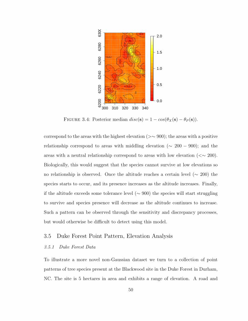
300 310 320 330 3406200

6220

6240

6260

6280

6300

0.0

0.5

1.0

1.5

2.0

Figure 3.4: Posterior median disc(s) = 1− cos(θX(s)− θP (s)).

correspond to the areas with the highest elevation (>∼ 900); the areas with a positive

relationship correspond to areas with middling elevation (∼ 200 − 900); and the

areas with a neutral relationship correspond to areas with low elevation (<∼ 200).

Biologically, this would suggest that the species cannot survive at low elevations so

no relationship is observed. Once the altitude reaches a certain level (∼ 200) the

species starts to occur, and its presence increases as the altitude increases. Finally,

if the altitude exceeds some tolerance level (∼ 900) the species will start struggling

to survive and species presence will decrease as the altitude continues to increase.

Such a pattern can be observed through the sensitivity and discrepancy processes,

but would otherwise be difficult to detect using this model.

3.5 Duke Forest Point Pattern, Elevation Analysis

3.5.1 Duke Forest Data

To illustrate a more novel non-Gaussian dataset we turn to a collection of point

patterns of tree species present at the Blackwood site in the Duke Forest in Durham,

NC. The site is 5 hectares in area and exhibits a range of elevation. A road and

50

powerline separate the site into three subregions, and we focus on the northwestern

of these subregions. We consider two tree species, Flowering Dogwood (Cornus

florida) and Sweetgum (Liquidambar styraciflua), with regard to their respective

point patterns of locations within the site in the year 2000. Some trees have multiple

stems observed at a single location; however we treat these as a single observed tree

at the given location. The point pattern for Sweetgum consists of 531 trees, and the

point pattern for Flowering Dogwood consists of 570 trees. Elevation is recorded at

each location where a tree of any species was observed, resulting in 5654 elevation

observations.

Figure 3.5 provides an interpolation of the elevation data. There is a clear increase

in elevation across the region in a roughly southeastern direction. Figure 3.5 also

provides the observed point patterns for each of the species. Flowering Dogwood

is well dispersed across the entire region while Sweetgum is more abundant in the

northwestern half of the region.

671800 671900

3983850

3983950

Easting

Nort

hin

g

671800 671900

3983850

3983950

Easting

Nort

hin

g

671800 671900

3983850

3983900

3983950

Easting

Nort

hin

g

160

162

164

166 168

170

172

174

176

1

78 160

165

170

175

180

Figure 3.5: From left to right, observed point patterns for Flowering Dogwood andSweetgum and observed elevation.

3.5.2 Point Pattern Model and Spatial Gradients

Given the observed elevation, X(s), we model the intensity for each species as a

log-Gaussian Cox process: λ(s) = exp(β0 + β1X(s))λ0(s), λ0(s) = exp(wz(s)), and

51

wz(s) ∼ GP (0, ρ(·|φz, σ2z)). Placing priors on the parameters, we have the following

model:

[Y |β0, β1, λ0(s), s ∈ D][λ0(s)|σ2, φ][β0, β1][φ][σ2]

= [Y |β0, β1, wz(s), s ∈ D][wz(s)|σ2, φ][β0, β1][φ][σ2]

where Y is the observed point pattern and λ0(s) is equivalently considered using

wz(s).

We approximate the likelihood by dividing the region into a fine grid with cells

Al; l = 1, . . . , L. This gives us the likelihood

L(λ(s), s ∈ D; s1, s2, . . . , sn) ≈ Πiλ(si) exp(−λ(D))

λ(D) ≈ Σl exp(X ′(Al)β + wz(Al))

where wz(Al) corresponds to a realization from a Gaussian process evaluated at

a representative point in each grid cell Al. This likelihood can be sampled using

elliptical slice sampling, as described in Murray et al. (2009) and Murray and Adams

(2010).

In terms of Z(s) = log(λ(s)), we immediately have a conditional bivariate GP

model with elevation: Z(s)|X(s) = β0 + β1X(s) + wz(s) and X(s) = α0 + wx(s)

with wz(s) ∼ GP (0, ρ(·|σ2z , φz)) and wx(s) ∼ GP (0, ρ(·|σ2

x, φx)). Hence, we are in the

framework developed in Chapter 2 and can apply the proposed gradient analyses.

The difference in this case will be that the Gaussian response Z(s) is latent and

thus unobserved. The uncertainty about Z(s) is propagated through the model by

drawing a posterior sample of the Z(s) surface for each posterior sample of the

parameters.

The methods developed in Chapter 2 allow for straight forward examination

of Dulogλ(s)/DuX(s) = DuZ(s)/DuX(s), although interest is more likely in the

behavior of the intensity surface itself. Applying the spatial gradient chain rule

52

discussed in Section 3.2 gives us Duλ(s) = exp(Z(s))DuZ(s), with the directional

derivative ratio Duλ(s)/DuX(s) = exp(Z(s))DuZ(s)/DuX(s). As before, we can

simplify this in terms of the independent Gaussian processes:

Duλ(s)

DuX(s)= exp(Z(s))

DuZ(s)

DuX(s)

=exp(Z(s))[β1Duwx(s) +Duwz(s)]

Duwx(s)

= exp(Z(s))[β1 +Duwz(s)

Duwx(s)]

The Cauchy random variable will again be centered at β1, but now there will also be

scaling according to the value of exp(Z(s)).

3.5.3 Results

Table 3.5.3 provides the fitted parameter values for elevation model. Tables 3.5.3

and 3.5.3 provide the fitted parameter values for each of the species models. Note

that the φz parameter is fixed at the minimum contrast estimate, as suggested in

Møller et al. (1998), to facilitate identifiability in the fitting of the log-Gaussian Cox

process. The fixed values are φz = 0.1063 and 0.0434 for Flowering Dogwood and

Sweetgum respectively. The 95% credible interval for β1 contains zero for Flowering

Dogwood, but not for Sweetgum. This negative coefficient suggests that the inten-

sity of Sweetgum decreases as elevation increases, while the intensity of Flowering

Dogwood is not responsive to elevation changes at this scale. Figure 3.6 provides the

posterior median intensity for each of the species. Both intensities have fairly low

values across most of the domain, with a few regions of higher intensity.

In Figure 3.5 we saw a clear increase in elevation in a roughly southeastern

direction. We approximate this direction by the unit vector u = (0.8508,−0.5255)

and consider the behavior of the directional derivative ratios in this direction for

53

671800 671850 671900 671950

3983850

3983900

3983950

0.0

1

0.02

0.02

0.02

0.03

0.03

0.04

0.04

0.04

0.0

4

0.0

5

0.0

6

671800 671850 671900 671950

3983850

3983900

3983950

0.02

0.0

2 0.04

0.04

0.0

4

0.06

0.0

6

0.08

0.08

0.1

0.05

0.10

0.15

Figure 3.6: Posterior median of the intensity surface for Flowering Dogwood (left)and Sweetgum (right).

Table 3.2: Parameter estimates for [X(s)] model for elevation.

Parameter 0.025 Mean 0.975α0 166.1043 167.8577 169.4328σ2x 7.1681 9.4117 12.9494φx 0.0791 0.0892 0.0979

each of the species. Figure 3.7 plots the resulting posterior median Duλ(s)/DuX(s)

surfaces.

For Flowering Dogwood the majority of the domain has a ratio close to zero. This

suggests that the changes in the intensity are negligible compared to the changes in

elevation. Recalling the fairly even spread of the trees in the region, as well as the

non-significant β1, this pattern makes sense.

For Sweetgum, virtually the entire region has a negative directional derivative

ratio. This aligns with our interpretation of the significantly negative β1 coefficient,

namely that as elevation increases the intensity decreases. There are a few subregions

where the change in intensity occurs more rapidly than elsewhere, and there is a larger

subregion where the change in intensity is zero due to an absence of trees. The cause

for subregions of rapid change could be further illuminated through examination

54

Table 3.3: Parameter estimates for [Z(s)|X(s)] model for Flowering Dogwood.

Parameter 0.025 Mean 0.975β0 -3.6416 -3.5478 -3.4590β1 -0.0866 -0.0284 0.0348σ2z 0.3367 0.5237 0.7648

Table 3.4: Parameter estimates for [Z(s)|X(s)] model for Sweetgum.

Parameter 0.025 Mean 0.975β0 -4.2161 -4.0297 -3.8728β1 -0.4094 -0.2619 -0.1024σ2z 0.7942 1.2652 1.9160

of other factors in those regions. Similarly, the region of zero change in intensity

could be roughly interpreted as Sweetgum having an aversion to elevations beyond

a certain value.

671800 671850 671900 671950

3983850

3983900

3983950

0

0

0

0

0

0

0

0

0

0

0 0

0

0.0

05

671800 671850 671900 671950

3983850

3983900

3983950

−0.0

3

−0.0

2

−0.0

2

−0.0

1

−0.01

−0.0

1

−0.0

1

−0.005

−0.0

05

0

−0.03

−0.02

−0.01

0.00

0.01

0.02

Figure 3.7: Posterior median of Duλ(s)/DuX(s) for Flowering Dogwood (left) andSweetgum (right); u = (0.8508,−0.5255).

Finally, we can compare the intensity and elevation surfaces by computing the

discrepancy between their directions of maximum gradient at each location, i.e., the

posterior median of disc(s) = 1− cos(θX(s)− θY (s)) across the region. Values close

to 2 suggest the surfaces are most rapidly increasing in opposite directions; values

55

671800 671850 671900 671950

3983850

3983900

3983950

0.8

0.8

1

1

1

1

1

1

1

1.2

1.2

1.2

1.4

1.4

1.4

1.4

1.6

1.6

671800 671850 671900 671950

3983850

3983900

3983950

1.5

1.6

1.6

1.6

1.7

1.75

1.8

1.8

1.8

1.8

5

1.85

1.9

1.9 1

.9

1.9

5

1.95

1.9

5

1.9

5

0.0

0.5

1.0

1.5

2.0

Figure 3.8: Posterior median disc(s) for Flowering Dogwood (left) and Sweetgum(right).

close to 0 suggest the surfaces are most rapidly increasing in the same direction.

The posterior median discrepancy surfaces are provided in Figure 3.8 for Flowering

Dogwood and Sweetgum.

The discrepancies for Flowering Dogwood roughly range between 0.8 and 1.5.

There is no clear pattern, which supports there being no strong relationship between

Flowering Dogwood intensity and elevation.

The pattern for Sweetgum is quite different. All of the discrepancies appear to be

between 1.5 and 2, with most around 1.9. This suggests that the Sweetgum intensity

and elevation are increasing in nearly opposite directions virtually everywhere in the

domain. This again confirms the negative relationship, and additionally highlights

this pattern as being slightly weaker in the northern part of the region.

3.6 Summary

Accounting for spatial dependence in observations can benefit analyses for a wide

array of real world data which, not surprisingly, will often require a non-Gaussian

first stage model. Many of these models will link a latent Gaussian process to the

56

response surface of interest through a differentiable function. As shown here, it is

straight forward to apply post model fitting gradient analysis in these cases through

the use of the spatial gradient chain rule. The resulting gradient analysis procedure

provides more localised inference regarding the relationship between the variables

without additional model fitting.

Several model structures exist for non-Gaussian data, several of which are dis-

cussed for binary data by Paciorek (2007). Here we show that the model choice will

have implications on the rates of change for the corresponding probability surfaces.

As demonstrated for a spatial probit regression, when using a thresholding approach

without a nugget term the rates of change will depend only on the rates of change

of the covariate surface. If a nugget term is incorporated into the model then the

rate of change will depend on both the rate of change for the latent Z(s) and the

covariate surface X(s). Finally, under a link function specification, the rate of change

will be similar to the thresholding model with a nugget, without the weighting of

1/√

1− σ2z . While similar, each model formulation suggests a distinct behavior for

the rates of change that may or may not be desirable. Similar differences can be

observed for other spatial GLMs.

To illustrate the gradient analysis in a spatial GLM framework we analyzed

presence-absence data coming from the CFR in South Africa requiring a binomial

first stage model. Standard inference procedures would involve examination of the

coefficient β1 to learn about the relationship with altitude as well as the spatial

P (s) surface to visualize the spatial distribution of the species. For these data,

the researcher would conclude that the species is positively associated with higher

altitudes. However, the local directional sensitivity process and spatial angular dis-

crepancy process tell a slightly different story. By highlighting more localized rela-

tionship patterns these processes reveal that the positive relationship with altitude

only occurs for certain levels of altitude, with the highest altitudes exhibiting a neg-

57

ative effect on species presence. Such conclusions regarding the range limits for the

species could have impacts on management decisions in the CFR.

Next, we applied gradient analyses to data where the response of interest was

a point pattern of trees from the Duke Forest modeled as a function of elevation

using a log-Gaussian Cox process. Using the local directional sensitivity process and

the spatial angular discrepancy process we studied the sensitivity of the intensity to

changes in elevation for two tree species. Only one of the two species is responsive

to changes in elevation, allowing for comparison of these gradient processes across

significant and non-significant regressions.

58

4

Gradient Analysis for Multivariate SpatialProcesses

4.1 Introduction

A common inferential aspect of spatial modeling is the resulting description of vari-

able relationships and how those relationships vary across a region. Post model

fitting gradient analyses can further illuminate these relationships, as described for

bivariate data in Chapter 2 and non-Gaussian data in Chapter 3. However, it is

well understood that no two variables will interact with one another in a vacuum,

completely independent of their surroundings. Instead, there will typically be a va-

riety of factors impacting the observed response at any location, and incorporating

these additional factors into a given model will have the potential to enhance our

understanding of these complex relationships. When these additional factors can rea-

sonably be modeled as a spatial surface they should be incorporated into the joint

spatial modeling, thus necessitating an extension of the gradient analysis procedures

to accommodate multivariate spatial processes.

The methodology proposed here will enable gradient analyses to be applied to

59

data where there may be several spatial response variables and/or several spatial

covariates of interest. In a bivariate example the only relationship that needs to be

explored is the dependence between response and covariate. In contrast, a multi-

variate example requires consideration of all response-covariate pairs, dependencies

which may all vary spatially in different ways. In addition, these pairwise dependen-

cies can be considered either marginally or conditional on the other model variables.

The gradient analyses provide further insight into these relationships as defined by

the joint model.

To illustrate this methodology we explore a dataset relating plant leaf traits and

climate in the Cape Floristic Region of South Africa. As described in Lamont et al.

(2002), within a plant family variation in leaf morphology will reflect the variable

environmental constraints on plant growth. Understanding these constraints and

how they vary across the region can provide insight into how plants may respond to

changes in climate. In our setup leaf traits are modeled jointly without assuming

any explicit dependence, as are temperature and precipitation, and all variables are

assumed to follow a spatial process model. This framework captures the correlation

between leaf traits which are not inherently independent since different trait mea-

surements are taken from a single individual. The dependence between leaf traits

and climate is explored first through the model parameters and later through the

gradient analyses.

The joint models and relevant gradient theory are detailed in Section 4.2; subsec-

tion 4.2.1 describes a single spatial response with multiple spatial covariates, subsec-

tion 4.2.2 describes multiple spatial responses with a single covariate, and subsection

4.2.3 describes multiple responses and multiple covariates. The data for the analyses

are described in Section 4.3. Results for the former two scenarios are provided in

Section 4.4. An overall summary is provided in Section 4.5.

60

4.2 Modeling Development

We consider the class of multivariate spatial coregionalization models and discuss

methodology for conducting gradient analyses within each setup. In particular, we

discuss three general frameworks for multivariate modeling: (1) one response with

multiple covariates, (2) multiple response variables with one covariate, and (3) mul-

tiple responses and multiple covariates. Each model implies a distribution for the

associated directional derivative processes which can be used to gain deeper insight

into the spatial relationships between the variables.

The processes are assumed, for convenience, to be weakly stationary such that

the covariance function C(s, s′) depends only on the separation vector δ = s − s′.

Specifically, we focus on isotropic covariance functions that depend only on the length

of the separation vector, ||δ||, and in our data examples the covariance function will

be assumed to be Matern with smoothness parameter ν = 3/2.

4.2.1 Multiple Predictors

Consider a response surface Y (s) : s ∈ R2 and two correlated covariate surfaces

X1(s), X2(s) : s ∈ R2. Let X(s) = (X1(s), X2(s))′ and X(s) = γ + AW(s),

where γ = (γ1, γ2)′, A is a symmetric 2× 2 matrix and W(s) = (w1(s), w2(s))′ is a

pair of independent zero-mean Gaussian processes with spatial covariance functions

G1(δ; 1, φ1) and G2(δ; 1, φ2) respectively. Note that the variance parameters in the

covariance functions are set to 1 for identifiability. Model the response surface con-

ditional on the covariates as a realization from a Gaussian process with covariance

function K(δ;σ2y, φy) such that E(Y (s)|X(s)) = X(s)β = β0 + β1X1(s) + β2X2(s).

Observed at a set of locations Y = (Y (s1), . . . , Y (sn)), we write Y|X ∼ N(Xβ,K)

and X ∼ N(γ,G1 ⊗A1 + G2 ⊗A2), where Gi is the covariance matrix associated

with wi and Ai = aia′i with ai the ith column of A.

61

Extending this model to accommodate additional predictor variables would be

straight forward, requiring an additional zero-mean Gaussian process wi(s) for each

additional variable. The general model for X(s) = (X1(s), X2(s), . . . , Xm(s))′ would

then be X ∼ N(γ,Σmi=1Gi ⊗Ai). Similarly, when appropriate, a differentiable func-

tion of one or more spatial covariates can be incorporated as an additional predictor.

It is straightforward to extend the chain rule to accommodate a multivariate func-

tion of spatial surfaces, such as an interaction term. For some differentiable function

g(X1(s), X2(s)) the associated directional derivative will be Dug(X1(s), X2(s)) =

dg(X1(s), X2(s))/dX1(s)×DuX1(s) + dg(X1(s), X2(s))/dX2(s)×DuX2(s). For ex-

ample, an interaction between the covariates, g(X1(s), X2(s)) = X1(s)X2(s), would

have a directional derivative Du(X1(s)X2(s)) = X1(s)DuX2(s) +X2(s)DuX1(s).

Prior distributions for the parameters completes the model specification. For the

β and γ parameters independent broad Normal priors are assumed. Inverse Gamma

distributions are used for the range parameters in the covariance functions φ1, φ2 and

φy, and similarly for the variance parameter σ2y in the covariance function for Y (s).

To understand the relationship between response and covariates there is interest

in sampling the associated directional derivatives DuY (s), DuX1(s), and DuX2(s).

In lieu of working with large joint multivariate Normal distributions, sampling these

derivatives is made more computationally convenient by captializing on independent

zero-mean spatial processes. With this goal, the above model can be written

Y (s) = β0 + β1X1(s) + β2X2(s) + wy(s) (4.1)

X1(s) = γ1 + a11w1(s) + a12w2(s)

X2(s) = γ2 + a12w1(s) + a22w2(s)

where wy(s), w1(s), and w2(s) are independent Gaussian processes. Given posterior

samples of the model parameters it is straight forward to sample the directional

derivative processes Duwi(s) marginally, thus avoiding any explosion in dimension.

62

Based on these samples, we can then compute the directional derivatives for the

response and covariates of interest.

The forms for the local directional sensitivity processes DuY (s)/DuX1(s) and

DuY (s)/DuX2(s) as functions of the independent Gaussian processes are provided

in (4.2) and (4.3).

DuY (s)

DuX1(s)= β1 +

β2DuX2(s) +Duwy(s)

DuX1(s)

= β1 +β2a12Duw1(s) + β2a22Duw2(s) +Duwy(s)

a11Duw1(s) + a12Duw2(s)(4.2)

DuY (s)

DuX2(s)= β2 +

β1DuX1(s) +Duwy(s)

DuX2(s)

= β2 +β1a11Duw1(s) + β1a12Duw2(s) +Duwy(s)

a12Duw1(s) + a22Duw2(s)(4.3)

In contrast to the single-covariate model, the sensitivities here exhibit dependence

in the ratio numerator and denominator. Understanding the distributional effects of

this dependence proves illuminating regarding the interpretation of the processes.

Recall that the sensitivities associated with the single-covariate model were cen-

tered at the parameter controlling the global relationship between the two variables.

A similar result can be obtained for the multi-covariate framework: If V ar(Duw1(s)) =

V ar(Duw2(s)), then the directional derivative ratios will be centered at the global

coefficients for X2(s) and X1(s). If the variances are not equal, then the cen-

tering for the ratios will be ‘close’ to the global coefficient, as a function of the

variance parameters. We define the global coefficient for Xi(s) as βi|xisuch that

E(Y (s)|Xi(s)) = β0|xi+ βi|xi

Xi(s); that is, it is the effect of the covariate Xi(s) after

marginalizing over the other covariate(s).

To illustrate this centering for DuY (s)/DuX1(s), consider the conditional expec-

63

tation of Y (s)|X1(s) using standard multivariate normal theory:

E(Y (s)|X1(s)) = β0 + β2γ2 −β2(a11a21 + a22a21)

a211 + a2

21

γ1 + (β1 +β2(a11a21 + a22a21)

a211 + a2

21

)X1

= β0|x1 + β1|x1X1(s) (4.4)

To see that this is the centering for the sensitivity, rewrite the ratio as follows:

DuY (s)

DuX1(s)=

(β1a11 + β2a21)Duw1(s) + (β1a21 + β2a22)Duw2(s) +Duwy(s)

a11Duw1(s) + a21Duw2(s)

=(β1a11 + β2a21)Duw1(s)

a11Duw1(s) + a21Duw2(s)+

(β1a21 + β2a22)Duw2(s)


+Duwy(s)

a11Duw1(s) + a21Duw2(s)(4.5)

The three ratios in (4.5) will be dependent Cauchy random variables. The third

ratio is centered at 0, and it can be shown that the first two ratios will be centered

at (β1a11/a21 + β2) a11/a21

a211/a

221+v22/v

21

and (β1a21/a11 + β2a22/a11) a21/a11

a221/a

211+v21/v

22

respectively,

where V ar(Duwi(s)) = v2i . Combining these terms, the overall centering for (4.5)

will be β1 +β2v21a11a21+v22a22a21

v21a211+v22a

221

. If v1 = v2, this centering will be equal to β1|x1 defined

in (4.4). An analogous result exists for X2.

In the case of the Matern covariance V ar(Duwi(s)) = φ2i , so centering at the

global coefficient will occur when the covariates share a common range parameter

φ1 = φ2.

This result provides an intuitive interpretation for the local directional sensitivity

processes. Parameter estimates from the model fitting will inform on the conditional

effects of each covariate, after accounting for the additional covariate(s). In a com-

plementary fashion, examination of the local directional sensitivities provides insight

into the marginal effect of the covariate across spatial and directional perspectives.

A hierarchical alternative to the model in (4.1) was elaborated in Royle and

Berliner (1999) and can be useful in scenarios where there is a natural ordering to

64

the variables. As described in Banerjee et al. (2004), the conditional multivariate

model can be viewed as a coregionalization model, X(s) = γ + AW(s), but arises

through specificication of A as an upper triangular matrix as opposed to the sym-

metric matrix described earlier. The general equivalence between the conditional and

unconditional specifications was shown in Banerjee et al. (2004), however the condi-

tional specification induces asymmetry in the local directional sensitivity processes

that may be undesirable when the variables have no inherent ordering.

Analogous computations for the conditional coregionalization model produce sim-

ilar inference and interpretations for the sensitivities. The model can be written,

Y (s) = β0 + β1X1(s) + β2X2(s) + wy(s) (4.6)

X2(s) = α0 + α1X1(s) + w2(s)

X1(s) = η0 + w1(s)

where wy(s), w1(s), and w2(s) are again independent Gaussian processes. Note, we

write w for notational purposes to differentiate the w1(s) and w2(s) processes from

the w1(s) and w2(s) processes.

Not surprisingly, the difference in model specification produces a difference in the

forms for the local directional sensitivity processes DuY (s)/DuX1(s) and

DuY (s)/DuX2(s), provided in (4.7) and (4.8).

DuY (s)

DuX1(s)= β1 +

β2DuX2(s) +Duwy(s)

DuX1(s)

= β1 + β2α1 +β2Duw2(s) +Duwy(s)

Duw1(s)(4.7)

DuY (s)

DuX2(s)= β2 +

β1DuX1(s) +Duwy(s)

DuX2(s)

= β2 + β1Duw1(s)

α1Duw1(s) +Duw2(s)+

Duwy(s)

α1Duw1(s) +Duw2(s)(4.8)

The ratio in (4.7) is a ratio of mean-zero independent Normal random variables,

65

similar to the sensitivity for the bivariate model. The sensitivity in (4.8) is written

as β2 plus a sum of two dependent ratios; the first ratio has dependence between

numerator and denominator, while the second is a ratio of two independent mean-

zero normal random variables.

Similar to the unconditional specification, under some conditions these sensitiv-

ities are centered at the global coefficients for the variables. The global coefficients

β1|x1 and β2|x2 are defined as

E(Y (s)|X1(s)) = (β0 + β2α0) + (β1 + β2α1)X1(s)

= β0|x1 + β1|x1X1(s) (4.9)

E(Y (s)|X2(s)) = (η0 −α1σ

21(α0 + α1η0)

α21σ

21 + σ2

2

) + (β2 + β1α1

α21 + u2

2/u21

)X2(s)

= β0|x2 + β2|x2X2(s) (4.10)

where V ar(wi(s)) = u2i .

It is immediately clear that the centering for (4.7) is equal to the global coefficient

defined in (4.9), and this centering does not depend on the variance parameters for

the processes. The centering for (4.8) as the global coefficient can be seen by showing

that the ratio Duw1(s)/(α1Duw1(s) +Duw2(s)) is centered at α1/(α21 + v2

2/v21) where

V ar(Duwi(s)) = v2i . Thus, the centering will be equal to the global coefficient if

v22/v

21 = u2

2/u21.

For a Matern covariance V ar(Duwi(s)) = u2iφ

2i , and equivalence will occur when

the covariates share a common range parameter φ1 = φ2. This is equivalent to the

result for the unconditional model, but here applies only to one of the two covariates.

When contemplating fitting a multivariate model under the conditional or uncon-

ditional specification it is important to consider whether the variables can reason-

ably be assumed to be ordered. The unconditional specification produces symmetric

inference for the two variables, with sensitivities centered at the global coefficient

66

contingent on the process variances. In contrast, under the conditional specification

the sensitivity for the variable modeled independently, X1(s) here, will always be cen-

tered at the global relationship parameter regardless of the process variances, while

the centering for the other sensitivity will be contingent on the process variances.

This asymmetry between the variables may be undesirable when no clear ordering

exists.

For either specification of the model one can additionally compute the spatial

angular discrepancy process associated with each of the covariates,

disc1(s) = 1− cos(θ1(s)− θy(s))

disc2(s) = 1− cos(θ2(s)− θy(s))

where θi(s) is the angle describing the direction of maximum gradient for the Xi(s) or

Y (s) surface at location s. These processes inform on the strength of the relationship

between variables, with a value of 0 indicating a strong positive relationship and

a value of 2 indicating a strong negative relationship. Because the directions of

maximum gradient are computed based on the full joint model, the interpretations

regarding the response-covariate relationships will be conditional on the additional

variables in the model.

4.2.2 Multiple Responses

Consider a pair of correlated response surfaces Y1(s), Y2(s) : s ∈ R2 that are both

dependent on a single covariate surface X(s) : s ∈ R2. Let Y(s) = (Y1(s), Y2(s))′

and Y(s) = γ +X(s)β +AW(s), where γ = (γ1, γ2)′, A is a symmetric 2×2 matrix

and W(s) = (w1(s), w2(s))′ is a pair of independent zero-mean Gaussian processes

with spatial covariance functions G1(δ; 1, φ1) and G2(δ; 1, φ2) respectively. The co-

variate surface is modeled as a spatially varying intercept using a Gaussian process

with covariance function K(δ;σ2y, φy) with some mean E(X(s)) = η0. Observed at

a set of locations Y = (Y(s1), . . . ,Y(sn)), we write Y|X ∼ N(γ + Xβ,G1 ⊗A1 +

67

G2 ⊗A2) and X ∼ N(η0,K). Similar to the multi-covariate version discussed in

4.2.1, this model can be extended to accommodate additional response variables

through the introduction of an additional zero-mean Gaussian process wi(s) for each

additional variable. The general model for Y(s) = (Y1(s), Y2(s), . . . , Ym(s))′ would

then be Y ∼ N(γ +Xβ,Σmi=1Gi ⊗Ai). Prior distributions for the parameters would

be comparable to those discussed in 4.2.1.

To facilitate computation of the directional derivatives DuY1(s), DuY2(s) and

DuX(s) the model is rewritten in terms of independent zero-mean Gaussian pro-

cesses,

Y1(s) = γ1 + β1X(s) + a11w1(s) + a12w2(s) (4.11)

Y2(s) = γ2 + β2X(s) + a12w1(s) + a22w2(s)

X(s) = η0 + wx(s)

where w1(s), w2(s) and wx(s) are independent Gaussian processes. This representa-

tion of the model allows us to easily compute the associated local directional sensi-

tivity processes,

DuY1(s)

DuX(s)= β1 +


Duwx(s)(4.12)

DuY2(s)

DuX(s)= β2 +


Duwx(s)(4.13)

Each of these sensitivities is a ratio of independent normal random variables and fol-

lows a Cauchy distribution centered at the parameter defining the global relationship

between response Yi(s) and the covariate X(s). In this case the global coefficient is

simply the coefficient of X(s) in the spatial linear model. This result is equivalent

to the result for the bivariate model.

The conditional specification for multiple-response data does not suffer from the

same asymmetry downfall as it does for the multiple-covariate data. However, the

68

dependence structure is inherited by the local directional sensitivities in a manner

that, again, may be undesirable when no inherent ordering of the responses exists.

The model can be written,

Y1(s) = β0 + β1Y2(s) + β2X(s) + w1(s) (4.14)

Y2(s) = α0 + α1X(s) + w2(s)

X(s) = η0 + wx(s)

where w1(s), w2(s) and wx(s) are mean-zero independen Gaussian processes. The

resulting sensitivities are

DuY2(s)

DuX(s)= α1 +

Duw2(s)

Duwx(s)(4.15)

DuY1(s)

DuX(s)= β2 + β1α1 +

β1Duw2(s) +Duw1(s)

Duwx(s)

= β2 + β1DuY2(s)

DuX(s)+Duw1(s)

Duwx(s)(4.16)

The above sensitivities are clearly centered at the parameters defining the global

relationships between response-covariate pairs, α1 and β1|x, where

E(Y1(s)|X(s)) = (β0 + β1α0) + (β2 + β1α1)X(s)

= β0|x + β1|xX(s) (4.17)

While there is no asymmetry in the centering of the sensitivities, the dependence

between the responses is apparent in the form of the sensitivity processes as shown

in (4.16). For the Y1(s) variable the local relationship with the covariate is depen-

dent on the spatial relationship of Y1(s) and X(s), but it is also dependent on the

spatial relationship between the covariate with the other response variable Y2(s). A

symmetric pattern does not hold true when examining the local relationship between

Y2(s) and the covariate, as shown in (4.15); the local relationship between X(s) and

Y2(s) depends only on the spatial structure of those two variables. This asymmetry

69

in the treatment of the response variables, and its desirability, should be taken into

account when specifying a multivariate model for multiple responses.

Once again, the directional derivatives can additionally be used to compute the

spatial angular discrepancy process associated with each of the responses and will

exhibit similar properties. We have

disc1(s) = 1− cos(θx(s)− θ1(s))

disc2(s) = 1− cos(θx(s)− θ2(s))

where θi(s) is the angle describing the direction of maximum gradient for the Yi(s) or

X(s) surface at any location s. The directions of maximum gradient are computed

based on surfaces from the joint model, so resulting inference will be conditional on

the other model variables.

4.2.3 Multiple Responses and Predictors

Consider a pair of correlated response surfaces Y1(s), Y2(s) : s ∈ R2 that are

dependent on a pair of correlated covariate surfaces X1(s), X2(s) : s ∈ R2. Let

Y(s) = (Y1(s), Y2(s))′ and X(s) = (X1(s), X2(s))′. Define the dependence between

response and covariate such that Y(s) = γ + X(s)β + AW(s), where γ = (γ1, γ2)′,

A is a symmetric 2× 2 matrix and W(s) = (w1(s), w2(s))′ is a pair of independent

zero-mean Gaussian processes with spatial covariance functions K1(δ; 1, φy1) and

K2(δ; 1, φy2) respectively. The covariate surfaces are modeled similarly such that

X(s) = η + BV(s), where η = (η1, η2)′, B is a symmetric 2× 2 matrix and V(s) =

(v1(s), v2(s))′ is a pair of independent zero-mean Gaussian processes with spatial

covariance functions G1(δ; 1, φx1) and G2(δ; 1, φx2). Observed at a set of locations

Y = (Y(s1), . . . ,Y(sn)), we write Y|X ∼ N(γ + Xβ,K1 ⊗A1 + K2 ⊗A2) and

X ∼ N(η,G1 ⊗B1 +G2 ⊗B2). Additional response and covariate variables can be

incorporated as discussed in Sections 4.2.1 and 4.2.2.

70

Directional derivatives DuY1(s), DuY2(s), DuX1(s) and DuX2(s) can be calcu-

lated using samples of the gradient processes for the independent zero-mean Gaussian

processes used to define the model,

Y1(s) = γ1 + β11X1(s) + β12X2(s) + a11w1(s) + a12w2(s) (4.18)

Y2(s) = γ2 + β21X1(s) + β22X2(s) + a12w1(s) + a22w2(s)

X1(s) = η1 + b11v1(s) + b12v2(s)

X2(s) = η2 + b12v1(s) + b22v2(s)

where w1(s), w2(s), v1(s) and v2(s) are independent Gaussian processes. Expressions

for computing the associated local directional sensitivities are similar to those in

Section 4.2.1 and are provided here for the Y1(s) process,

DuY1(s)

DuX1(s)= β11 +

β12DuX2(s) + a11Duw1(s) + a12Duw2(s)

DuX1(s)

= β11 +β12b11Duv1(s) + β12b12Duv2(s) + a11Duw1(s) + a12Duw2(s)

b11Duv1(s) + b12Duv2(s)(4.19)

DuY1(s)

DuX2(s)= β12 +

β11DuX1(s) + a11Duw1(s) + a12Duw2(s)

DuX2(s)

= β12 +β11b12Duv1(s) + β11b22Duv2(s) + a11Duw1(s) + a12Duw2(s)

b12Duv1(s) + b22Duv2(s)(4.20)

Sensitivities for the Y2(s) process are analogous.

Using arguments similar to those in Section 4.2.1 it can be shown that these ratios

will be centered at the global coefficients relating each covariate to each response

variable. The global coefficient relating Y1(s) and X1(s) is defined as βy11|x1, where

E(Y1(s)|X1(s)) = (γ1 + β12η2 − β12b11b12 + b22b12

b211 + b2

12

η1) + (β11 +b11b12 + b22b12

b211 + b2

12

)X1(s)

= βy10|x1 + βy1

1|x1X1(s)

71

Global coefficients relating the other responses and covariates can be computed in

the same manner.

There will be a spatial angular discrepancy process associated with each pair of

response and covariate,

disc11(s) = 1− cos(θx1(s)− θy1(s))




where θxi(s) and θyi(s) are the angles describing the direction of maximum gradient

for the Yi(s) or Xi(s) surface at location s. The spatial angular discrepancies hold

similar properties as described earlier, and will again provide inference conditional

on the variables included in the joint model.

4.3 Multivariate Examples using South African Plant Traits

4.3.1 Data

A dataset coming from the Cape Floristic Region in South Africa is used to illustrate

the gradient analyses outlined in Sections 4.2.1 and 4.2.2 for models with multiple

covariates or multiple responses of interest. The data was collected for 37 plant

species in the genus Protea in order to assess plant trait patterns associated with

environmental covariates in the region. Data are available from 36 plots, with inter-

plot distances ranging from 78 to 366,100 meters apart. Figure 4.1 provides the plot

locations. The poor spatial spread of the plots prevents any meaningful inference on

the shape of the spatial surfaces, but the multivariate nature of the data lends itself

to illustrating the gradient methodology for multiple predictors or responses. Within

each plot leaf trait measurements are available for one or more Protea species, with

the total number of plants measured per plot ranging from 5 to 24. Many species are

72

only available in a single plot, and generally 8 individuals are sampled within each

species.

Easting

Nor

thin

g

6200

000

6240

000

6280

000

300000 400000 500000 600000

Figure 4.1: Plot locations for Cape Floristic Region leaf trait data.

As response variables we consider two plant traits, leaf dry mass per unit area

(LMA) and leaf fresh water content (FWC). LMA (multiplied by 100 for convenience)

ranges between 0.7 and 8.9 with plot-level averages between 1.3 and 4.6. FWC

ranges between 0.5 and 3.7 with plot-level averages between 0.9 and 2.4. See the top

row of Figure 4.2 for associated histograms. As covariates we consider two climate

variables, mean annual temperature (MAT) and mean annual precipitation (MAP).

MAT ranges between 11 and 18 degrees Celsius, and MAP ranges between 331 and

1332. See the bottom row of Figure 4.2 for associated histograms.


To illustrate a multiple-covariate model let the response variable Y (s) be leaf mass

per area (LMA), and the covariates X1(s) and X2(s) be mean annual temperature

(MAT) and mean annual precipitation (MAP). As described in Section 4.3.1, sev-

eral measurements are available for the response variable at each location. Denote

these observations as Yi(s) for i = 1, . . . , ns, where ns is the number of observations

available at location s. These data are jointly modeled using a coregionalization

73

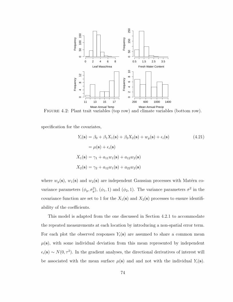
Leaf Mass/Area

Fre

quen

cy

0 2 4 6 8

050

100

150

Fresh Water Content

Fre

quen

cy

0.5 1.5 2.5 3.5

050

150

250

Mean Annual Temp

Fre

quen

cy

11 13 15 17

04

812

Mean Annual Precip

Fre

quen

cy

200 600 1000 1400

02

46

810

Figure 4.2: Plant trait variables (top row) and climate variables (bottom row).

specification for the covariates,

Yi(s) = β0 + β1X1(s) + β2X2(s) + wy(s) + εi(s) (4.21)

= µ(s) + εi(s)

X1(s) = γ1 + a11w1(s) + a12w2(s)

X2(s) = γ2 + a12w1(s) + a22w2(s)

where wy(s), w1(s) and w2(s) are independent Gaussian processes with Matern co-

variance parameters (φy, σ2y), (φ1, 1) and (φ2, 1). The variance parameters σ2 in the

covariance function are set to 1 for the X1(s) and X2(s) processes to ensure identifi-

ability of the coefficients.

This model is adapted from the one discussed in Section 4.2.1 to accommodate

the repeated measurements at each location by introducing a non-spatial error term.

For each plot the observed responses Yi(s) are assumed to share a common mean

µ(s), with some individual deviation from this mean represented by independent

εi(s) ∼ N(0, τ 2). In the gradient analyses, the directional derivatives of interest will

be associated with the mean surface µ(s) and and not with the individual Yi(s).

74

Otherwise, the local directional sensitivities will be as described in Section 4.2.1


To illustrate a multiple-response model consider Y1(s) as leaf mass per area (LMA)

and Y2(s) as fresh water content (FWC), with the covariate mean annual temperature

(MAT) as X(s). As described above, the response variables have several measure-

ments at each location, accommodated through the introduction of a non-spatial

error term ε(s). The subsequent gradient analyses then consider the relationship

between the mean responses µ1(s) and µ2(s) and the covariate. The model is written

using a coregionalization specification for the responses,

Y1i(s) = β0 + β1X(s) + a11w1(s) + a12w2(s) + ε1i(s) (4.22)

= µ1(s) + ε1i(s)

Y2i(s) = α0 + α1X(s) + a12w1(s) + a22w2(s) + ε2i(s)

= µ2(s) + ε2i(s)

X(s) = η0 + wx(s)

where w1(s), w2(s) and wx(s) are independent Gaussian processes with Matern co-

variance parameters (φ1, 1), (φ2, 1), and (φx, σ2x). The variance parameters σ2 for the

Yi(s) processes are set to 1 for identifiability.

The local directional sensitivity processes are as described in Section 4.2.2, except

that they are now associated with Duµ1(s)/DuX(s) and Duµ2(s)/DuX(s).

4.4 Results


Posterior means and 95% credible intervals for the model parameters in (4.21) are

provided in Table 4.1. Estimates are based on 5000 samples, after a burn-in of

1000 iterations and a thinning of every 10th iterate. The credible intervals for both

75

covariates overlap zero, but MAT appears to have a more meaningful effect than

MAP. The point estimate for MAP is effectively zero and the interval is nearly

symmetric around zero, suggesting no effect on LMA. The posterior mean kriged

surfaces for the three variables X1(s), X2(s) and µ(s) are provided in Figure 4.3 and

exhibit limited spatial structure as a result of the spatial spread in the observed data.

Table 4.1: Parameter estimates and 95% credible intervals for the [Y |X1, X2][X1, X2]model.

Estimate q0.025 q0.975

β0 4.3206 1.4759 7.3492β1 -0.0840 -0.2793 0.1079β2 0.000007 -0.0012 0.0012σ2y 0.3323 0.0534 0.9328φy 0.0006 0.0004 0.0010τ 2y 4.7344 2.0621 9.0188

γ1 16.0338 15.0630 16.9828γ2 750.67 635.32 867.65a11 2.0258 1.5109 2.7432a12 0.4181 -0.2952 1.1540a22 249.50 199.54 314.76φ1 0.0007 0.0005 0.0010φ2 0.0005 0.0004 0.0007

Figure 4.3: Posterior mean kriged surfaces for X1(s), X2(s), and µ(s) from left toright.

The posterior median local directional sensitivity surfaces and spatial angular

discrepancy surfaces are provided in Figure 4.4. Unfortunately, the limited spatial

spread in the observed data prevents illumination of any spatial story, but the pro-

cesses enable general comparisons between the response variable and each of the

76

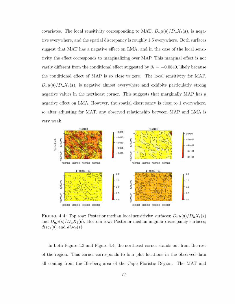
covariates. The local sensitivity corresponding to MAT, Duµ(s)/DuX1(s), is nega-

tive everywhere, and the spatial discrepancy is roughly 1.5 everywhere. Both surfaces

suggest that MAT has a negative effect on LMA, and in the case of the local sensi-

tivity the effect corresponds to marginalizing over MAP. This marginal effect is not

vastly different from the conditional effect suggested by β1 = −0.0840, likely because

the conditional effect of MAP is so close to zero. The local sensitivity for MAP,

Duµ(s)/DuX2(s), is negative almost everywhere and exhibits particularly strong

negative values in the northeast corner. This suggests that marginally MAP has a

negative effect on LMA. However, the spatial discrepancy is close to 1 everywhere,

so after adjusting for MAT, any observed relationship between MAP and LMA is

very weak.

300000 400000 500000 600000

6200

000

6260

000

Dµ/DX1

Nor

th/S

outh

−0.090

−0.085

−0.080

−0.075

−0.070

−0.

086

−0.086

−0.086

−0.

086

−0.086

−0.086

−0.084

−0.084 −0.084

−0.084

−0.084

−0.082

−0.082

−0.082 −0.082

−0.082

−0.082

−0.082

−0.082

−0.

082

−0.08

−0.08

−0.08

−0.08

−0.078

300000 400000 500000 600000

6200

000

6260

000

Dµ/DX2

−8e−04

−6e−04

−4e−04

−2e−04

0e+00

−1e−04

−1e−04

−1e−04

−1e−04

−1e−04

−1e−04

−1e−04

300000 400000 500000 600000

6200

000

6260

000

1−cos(θ1−θy)

0.0

0.5

1.0

1.5

2.0 1.52

1.52

1.52

1.52

1.52

1.52

1.52

1.52

1.54

1.54

1.54

1.54

1.54

1.54

300000 400000 500000 600000

6200

000

6260

000

1−cos(θ2−θy)

0.0

0.5

1.0

1.5

2.0

1.0

4

1.06

1.0

6

1.06

1.06

1.06

1.06

1.06

1.0

6

1.06

1.06

1.08

1.08 1.08

1.08

1.08

1.08

1.08

1.08

1.0

8

1.08

1.08

1.1

Figure 4.4: Top row: Posterior median local sensitivity surfaces; Duµ(s)/DuX1(s)and Duµ(s)/DuX2(s). Bottom row: Posterior median angular discrepancy surfaces;disc1(s) and disc2(s).

In both Figure 4.3 and Figure 4.4, the northeast corner stands out from the rest

of the region. This corner corresponds to four plot locations in the observed data

all coming from the Blesberg area of the Cape Floristic Region. The MAT and

77

MAP for the Blesberg plots are lower than for any other plots in the data, while the

LMA measurements are close to average. The highlighting of this area in the local

directional sensitivity for MAP indicates that the relationship between LMA and

MAP is atypical in this region. This can most easily be seen through comparison

with the southwest corner. The two areas have similar LMA, but correspond to

opposite extremes for MAP. Since the data in the southwest corner aligns more

closely with the rest of the data, the northwest corner is highlighted in the local

directional sensitivity.


Posterior means and 95% credible intervals for the parameters in the model (4.22)

are provided in Table 4.2. Estimates are based on 5000 samples after a burn-in of

1000 iterations and a thinning of every 10th iterate. The credible intervals for β1 and

α1, relating each response variable to MAT, both overlap zero. However, the point

estimates suggest MAT has a small negative effect on LMA and a small positive

effect on MAP. The three posterior mean kriged surfaces for µ1(s), µ2(s) and X1(s)

are provided in Figure 4.5, and again display limited spatial structure.

Figure 4.5: Posterior mean kriged surfaces for X, µ1, and µ2 from left to right.

The posterior median local directional sensitivities and spatial angular discrep-

ancies are provided in Figure 4.6. As expected, the local sensitivity for LMA,

Duµ1(s)/DuX(s), is roughly centered at β1 = −0.0725, the parameter defining

the variables’ relationship. The poor spatial structure of the observed data pre-

78

Table 4.2: Parameter estimates and 95% credible intervals for the [Y1, Y2|X][X]model.

Estimate q0.025 q0.975

β0 4.1415 1.1574 7.1401β1 -0.0725 -0.2629 0.1147α0 0.5275 -0.8393 1.7569α1 0.0502 -0.0251 0.1350a11 0.4567 0.0303 1.0044a12 -0.1501 -0.4203 0.0676a22 0.1812 0.0101 0.4064τ 2

1 5.0906 2.1198 9.7001τ 2

2 0.5453 0.1566 1.2413φ1 0.0006 0.0004 0.0009φ2 0.0006 0.0004 0.0010η0 16.0486 14.9481 17.0768φx 0.0006 0.0004 0.0009σ2x 5.3382 2.3916 11.5144

vents meaningful spatial variation beyond this centering. The angular discrepancy

disc1(s) takes values close to 1.5, indicating a relatively strong negative relationship.

The results for FWC are similar, but indicate a positive relationship. The local

sensitivity Duµ2(s)/DuX(s) is roughly centered at α1 = 0.0502 with no meaningful

spatial structure, and the angular discrepancy disc2(s) takes values of approximately

0.45 indicating a fairly strong positive relationship.

It’s not surprising that the local directional sensitivity for LMA looks similar to

the sensitivity Duµ(s)/DuX1(s) in Figure 4.4 since both are describing the marginal

effect of MAT on LMA. In this model MAT is the only covariate, while in the earlier

model the local directional sensitivity was expected to be centered at the marginal

effect of MAT after marginalizing over MAP. The similarity between these figures

confirms the theoretical result.

79

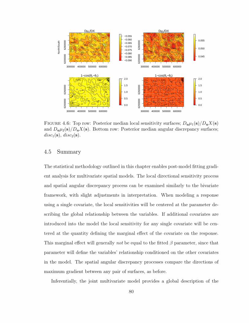
300000 400000 500000 60000062

0000

062

6000

0

Dµ1/DX

Nor

th/S

outh

−0.090−0.085−0.080−0.075−0.070−0.065−0.060−0.055

−0.075

−0.

07

−0.

07

−0.07

−0.07

−0.07

−0.07

−0.07

−0.07

−0.07

300000 400000 500000 600000

6200

000

6260

000

Dµ2/DX

0.045

0.050

0.055

0.046

0.046

0.048

0.048

0.048

0.048

0.048

0.05

0.05

0.05

0.05 0.05

0.05

300000 400000 500000 600000

6200

000

6260

000

1−cos(θx−θ1)

0.0

0.5

1.0

1.5

2.0

1.46

1.46

1.46 1.46

1.46

1.48

1.48

1.48

1.48

1.48

1.48

1.5

1.5

300000 400000 500000 600000

6200

000

6260

000

1−cos(θx−θ2)

0.0

0.5

1.0

1.5

2.0 0.4

0.42

0.42

0.42

0.4

4

0.44

0.44

0.44

0.44

0.44

0.44

0.44

0.44

0.44

Figure 4.6: Top row: Posterior median local sensitivity surfaces; Duµ1(s)/DuX(s)and Duµ2(s)/DuX(s). Bottom row: Posterior median angular discrepancy surfaces;disc1(s), disc2(s).

4.5 Summary

The statistical methodology outlined in this chapter enables post-model fitting gradi-

ent analysis for multivariate spatial models. The local directional sensitivity process

and spatial angular discrepancy process can be examined similarly to the bivariate

framework, with slight adjustments in interpretation. When modeling a response

using a single covariate, the local sensitivities will be centered at the parameter de-

scribing the global relationship between the variables. If additional covariates are

introduced into the model the local sensitivity for any single covariate will be cen-

tered at the quantity defining the marginal effect of the covariate on the response.

This marginal effect will generally not be equal to the fitted β parameter, since that

parameter will define the variables’ relationship conditioned on the other covariates

in the model. The spatial angular discrepancy processes compare the directions of

maximum gradient between any pair of surfaces, as before.

Inferentially, the joint multivariate model provides a global description of the

80

response-covariate pairwise relationships, conditional on the remaining set of vari-

ables. The post model-fitting gradient analyses expand on this description and com-

pare the spatial variation in these relationships across variables. Similar to the

model parameters, the spatial angular discrepancies inform on the sign and strength

of pairwise behaviors conditional on the other covariates, while the local directional

sensitivities inform on the marginal relationships between response and covariate.

Together, these quantities provide a fuller picture of the dependencies suggested by

the joint model.

The development in Section 4.2.1 highlights the importance of model choice for

coregionalization models. Banerjee et al. (2004) showed that the unconditional (sym-

metric) and conditional (upper triangular) specifications can be considered reparam-

eterizations of the same model, but inference regarding rates of change will vary

under the two models. The unconditional model treats the variables identically, each

dependent on the other, and this is apparent in the resulting directional derivatives.

Under the conditional model, one variable is modeled independently from the other

and again this shows in the resulting directional derivatives. When a clear ordering

exists between the variables, a conditional model will be a reasonable choice, but if

no obvious ordering can be assumed then the unconditional model will provide the

desired symmetric treatment of the variables.

The methodology was demonstrated for plant trait and climate data coming

from the Cape Floristic Region in South Africa, illustrating both a multiple-response

model and a multiple-covariate model. The presence of several correlated response

variables (plant traits) and several correlated covariates (climate variables) in these

data necessitated the use of multivariate spatial models. The plant trait measure-

ments cannot reasonably be assumed independent from one another, nor can one

sensibly assign an order of dependence to the traits, so a coregionalization model

with a symmetric specification was deemed most appropriate for their joint model.

81

A similar reasoning regarding temperature and precipitation encouraged a similar

model be used for their joint model.

A few benefits of the gradient analysis were highlighted in the multiple-covariate

model, where leaf mass per area is assumed to be a function of precipitation and

temperature. Although the fitted model suggests that there is no real relationship

with precipitation after adjusting for temperature, the local directional sensitivity

suggests that marginally precipitation would have a negative effect. This negative

effect is in line with results described by Lamont et al. (2002). The fitted model

also suggested a negative effect for temperature, both marginally and conditional on

precipitation. This is also in line with current literature, as described in Poorter

et al. (2009). The local sensitivities additionally highlighted the Blesberg region as

potentially behaving differently from the other locations, a difference that could be

further investigated if deemed to be of interest.

82

5

Additional Gradient Analysis Extensions

5.1 Spatial-Temporal Modeling

5.1.1 Introduction

In addition to spatial structure, many researchers will be interested in learning how

variable relationships evolve temporally. A readily available environmental example

would be measurements of ozone and temperature, which are often available on a

daily time scale. Accommodating such data requires flexible models allowing for

both spatial and temporal dynamics, which have a rich presence in the literature

(e.g. Wikle et al., 1998; Banerjee et al., 2004; Gelfand et al., 2005; Cressie and Wikle,

2011; Reich et al., 2011b). So called “separable” models can be factored into a purely

spatial component and a purely temporal component. This is generally undesirable

because it does not allow for space-time interactions that would be expected for

many data. The class of “non-separable” models are more complicated to fit but

allow for more complex spatial-temporal dynamics to be captured since they cannot

be factored in the same way. In addition, models can be classified based on whether

they discretize space and/or time, with continuous space and discrete time perhaps

83

most common.

Process gradients were recently explored for spatial-temporal models by Quick

et al. (2013) to identify time points with significantly high residual gradients that

would suggest a missing covariate. The scenario they consider involves temporal

gradients in the continuous time and discrete space setting. In contrast, the method-

ology we propose examines spatial gradients in the discrete time and continuous space

setting. Their methodology assesses temporal gradients after adjusting for spatial ef-

fects, while ours assesses spatial gradients after adjusting for temporal effects. Either

approach may be desirable depending on the setting.

To illustrate spatial gradient analyses for spatial-temporal models we consider

three fairly basic forms for a spatial-temporal error term with increasing complexity.

In addition to the relative rate of change between response-covariate pairs, the tem-

poral setting enables comparisons of the relative rates of change for a single surface

at multiple time points. This time-lag comparison provides insight into the temporal

evolution for the surface’s rate of change.

5.1.2 Modeling and Gradient Theory

Consider a response Y (s, t) and covariate X(s, t) each observed at a set of locations

s1, . . . , sn and a set of time points t1, . . . , tm. Assume the following joint spatial-

temporal model,

Y (s, t) = β0 + β1X(s, t) + ey(s, t) (5.1)

X(s, t) = α0 + ex(s, t)

84

The error terms for the Y (s, t) and X(s, t) processes capture the spatial and temporal

dependence in one of three ways:

e(s, t) = η(t) + w(s) (5.2)

e(s, t) = w(t)(s) (5.3)

e(s, t) = v(s, t) (5.4)

The error structure in (5.2) assumes independent spatial and temporal effects where

w(s) ∼ GP (0, ρ(·)) is shared across all time points and η(t) = η(t − 1) + ε(t) with

iid ε(t) ∼ N(0, τ 2). Next, the error structure in (5.3) assumes a unique independent

spatial effect at each time point with w(t)(s) ∼ GP (0, ρ(·)). Finally, the error struc-

ture in (5.4) allows for a spatial and temporal evolution at each time point such that

v(s, t) = v(s, t − 1) + w(t)(s) + ε(t) with w(t)(s) and ε(t) defined as in the previous

models.

Note, a pure (non-spatial and non-temporal) error component could be added to

any of the above error structures, but for the gradient analyses would be ignored

with directional derivatives being calculated on the remaining smooth surface.

Spatial gradients can be computed for each of the models described above and

not surprisingly inherit the characteristics present in the parent model. Similar to

the non-temporal models discussed in previous chapters, these can then be used to

compute the local directional sensitivities comparing the the spatial rates of change at

any given time point. In addition, local directional time-lag ratios can be considered

for each variable, and may give insight into how the surface’s rates of change vary

over time.

The local directional sensitivities at time t under each of the three error structures

85

will be

DuY (s, t)

DuX(s, t)= β1 +

Duwy(s)

Duwx(s)

DuY (s, t)

DuX(s, t)= β1 +

Duw(t)y (s)

Duw(t)x (s)

DuY (s, t)

DuX(s, t)= β1 +

Duvy(s, t)

Duvx(s, t)

All three local directional sensitivities will be Cauchy distributed centered at the

global relationship parameter β1. The Cauchy distribution can be seen by observing

that in each case the ratio term in the sensitivity will involve two mean-zero indepen-

dent normal random variables. The local directional sensitivity for (5.2) is constant

through time, reflecting the time-invariant spatial error. Similarly, the sensitivity for

(5.3) varies at each time point, but is independent across time. For (5.4), the autore-

gressive nature of the error function is inherited by the local directional sensitivity

process. Substituting terms according to the definition of v(s, t) we have

DuY (s, t)

DuX(s, t)=β1 +

Duvy(s, t− 1)

Duvx(s, t− 1)

+Duvx(s, t− 1)Duw

(t)y (s)−Duvy(s, t− 1)Duw

(t)x (s)

Duvx(s, t− 1)(Duvx(s, t− 1) +Duw(t)x (s))

=DuY (s, t− 1)

DuX(s, t− 1)+Duvx(s, t− 1)Duw

(t)y (s)−Duvy(s, t− 1)Duw

(t)x (s)

Duvx(s, t− 1)(Duvx(s, t− 1) +Duw(t)x (s))

with the error term centered at zero.

The local directional time-lag ratios are uninteresting for (5.2) and (5.3) since

neither model allows the spatial errors to evolve in time. Focusing on the third

error structure, (5.4), the local directional time-lag ratio can be computed in two

scenarios. First, when the mean is non-dynamic (i.e., X(s, t) is not jointly modeled)

86

and interest is only in the behavior of the residual,

Duet(s)

Duet−1(s)=

Duv(s, t)

Duv(s, t− 1)

= 1 +Duw

(t)(s)

Duv(s, t− 1)

and second, when the covariate X(s, t) is jointly modeled,

DuYt(s)

DuYt−1(s)=

β1DuX(s, t) +Duvy(s, t)

β1DuX(s, t− 1) +Duvy(s, t− 1)

=DuXt(s)

DuXt−1(s)+β1DuX(s, t− 1)Duvy(s, t)− β1DuX(s, t)Duvy(s, t− 1)

β1DuX(s, t− 1)(β1DuX(s, t− 1) +Duvy(s, t− 1))

In both scenarios the local directional time-lag ratio will be centered at 1, with some

zero-centered error term. This is consistent with the belief that the rate of change

for the spatial surface should roughly stay constant from year to year.

The examples provided here give some insight into the kinds of spatial gradients

that can be examined in a spatial-temporal setting. Characteristics from the parent

model will generally be inherited by the gradient processes, and the complexity of the

gradient functions will depend on the complexity of the original model. We propose

examination of both local directional sensitivities at a given time point, and local

directional time-lag ratios across time points to gain a deeper understanding of the

processes involved.

5.2 Data with Spatial Misalignment

5.2.1 Introduction

When collecting data for environmental or ecological studies there will often be

spatial misalignment between measurements for climate variables and measurements

for plant or animal characteristics. For example, observations for bud-burst will occur

at the location of individual trees while temperature observations may be taken from

87

the nearest weather monitoring station or may correspond to the average temperature

in a relevant spatial unit. Misalignment in the covariate and response observations,

or between the observed spatial scale and desired inferential spatial scale, can inject

errors and biases into the analysis. Several approaches have been proposed in the

literature to accommodate such data (e.g. Mugglin et al., 2000; Gotway and Young,

2002; Banerjee et al., 2004; Gryparis et al., 2009; Peng and Bell, 2010).

Following discussions by Banerjee et al. (2004), we accommodate areal data by

treating them as block averages across the region. This interpretation is appropriate

for several potential climate measurements such as average temperature or precip-

itation, as well as potential environmental responses such as pollution. Areal data

clearly do not constitute a smooth surface for which rates of change can be consid-

ered, a requirement for the gradient analyses presented thus far. Instead, we use the

areal observations to make predictions at new point-referenced locations based on a

Gaussian process model and the block average interpretation of the areal observa-

tions. This in turn allows for consideration of the rate of change for the corresponding

surface, including comparisons with the rate of change for the response surface.

Here we illustrate how gradient analyses can be applied under three misalign-

ment scenarios. The first is most straight forward and involves two point-referenced

variables, response and covariate, that do not share a common set of observation lo-

cations. The second applies to scenarios when the covariate is only available as areal

data, interpreted as a block average, and the response is point-referenced. Scenarios

where the response is block averaged and the covariate is point-referenced would fol-

low similarly. The final scenario assumes both the response and covariate are block

average data.

88


The methodology and notation for the misalignment scenarios follow those proposed

by Banerjee et al. (2004).

For the first scenario we assume that the covariate and response variables were

observed at different locations, e.g. tree locations vs. monitoring station locations.

To understand the variables’ relationship we would ideally have paired measurements,

allowing the response to be regressed on corresponding covariate values at the same

location. Instead, we observe the response Y (s) at a set of locations Sy = s1, . . . , sn

and the covariate at a non-identical set of locations Sx = s′1, . . . , s′m. Consider a

spatially varying intercept model

X(s′) = α + wx(s′)

wx(s′) ∼ GP (0, ρx(σ

2x, φx))

Letting Xs = X(s) : s ∈ Sy and Xs′ = X(s′) : s′ ∈ Sx, we can sample covariate

values at the desired locations (i.e., the locations where Y (s) was observed) using

the predictive distribution

f(Xs|Xs′) =

∫f(Xs|Xs′ , α, σ

2x, φx)f(α0, σ

2x, φx|Xs′)dαdσ

2xdφx

The spatial regression can be fit such that

Y (s) = β0 + β1X(s) + wy(s)

wy(s) ∼ GP (0, ρy(σ2y , φy))

where Y (s) and X(s) are both mean square differentiable processes, and the model

likelihood is

[Y (s)|X(s),β, σ2y , φy][X(s)|X(s′), α, σ2

x, φx][X(s′)|α, σ2x, φx][θ]

with [θ] the prior distribution for the collection of model parameters.

89

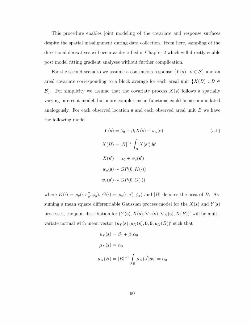
This procedure enables joint modeling of the covariate and response surfaces

despite the spatial misalignment during data collection. From here, sampling of the

directional derivatives will occur as described in Chapter 2 which will directly enable

post model fitting gradient analyses without further complication.

For the second scenario we assume a continuous response Y (s) : s ∈ S and an

areal covariate corresponding to a block average for each areal unit X(B) : B ∈

B. For simplicity we assume that the covariate process X(s) follows a spatially

varying intercept model, but more complex mean functions could be accommodated

analogously. For each observed location s and each observed areal unit B we have

the following model

Y (s) = β0 + β1X(s) + wy(s) (5.5)

X(B) = |B|−1

∫B

X(s′)ds′

X(s′) = α0 + wx(s′)

wy(s) ∼ GP (0, K(·))

wx(s′) ∼ GP (0, G(·))

where K(·) = ρy(·;σ2y, φy), G(·) = ρx(·;σ2

x, φx) and |B| denotes the area of B. As-

suming a mean square differentiable Gaussian process model for the X(s) and Y (s)

processes, the joint distribution for (Y (s), X(s),∇Y (s),∇X(s), X(B))′ will be multi-

variate normal with mean vector (µY (s), µX(s),0,0, µX(B))′ such that

µY (s) = β0 + β1α0

µX(s) = α0

µX(B) = |B|−1

∫B

µX(s′)ds′ = α0

90

and cross-covariance matrix

V (δ, Bi, Bj) =

K(δ) β1G(δ) −∇K(δ)′ −β1∇G(δ)′ β1Gs,B

β1G(δ) G(δ) −β1∇G(δ)′ −∇G(δ)′ Gs,B

∇K(δ) β1∇G(δ) −HK(δ) −β1HG(δ) −β1∇GB

β1∇G(δ) ∇G(δ) −β1HG(δ) −HG(δ) −∇GB

β1Gs,B Gs,B β1∇GB ∇GB GB

(5.6)

where δ = s − s′ and Cov(Y (s), Y (s′)) = K(δ) = K(δ) + β2G(δ). As in Chapter

2, ∇G(δ) is the 2× 1 gradient vector associated with G(δ), and HG(δ) is the 2× 2

Hessian matrix associated with G(δ). We define the components corresponding to

the block averages,

(GB)ij = |Bi|−1|Bj|−1

∫Bi

∫Bj

ρx(si − sj;σ2x, φx)dsidsj

(Gs,B)s,j = |Bj|−1

∫Bj

ρx(s− sj;σ2x, φx)dsj

(∇GB)s,j = (|Bj|−1

∫Bj

(∇G(s− sj))1dsj, |Bj|−1

∫Bj

(∇G(s− sj))2dsj)′

I.e., for each location s and each block Bj, (∇GB)s,j is a 2×1 vector such that element

i corresponds to the ith element of ∇G(s− sj) block averaged over all sj ∈ Bj.

In practice the above integrals are approximated using Monte Carlo integration.

For each block Bj draw a set of Lj locations sj1, . . . , sjLjuniformly across the region,

with the number of locations Lj adjusted to be appropriate for the block size. The

approximations are then

(GB)ij = L−1i L−1

j ΣlΣmρx(sil − sjm;σ2x, φx) (5.7)

(Gs,B)s,j = L−1j Σlρx(s− sjl;σ

2x, φx)

(∇GB)s,j = (L−1j Σl(∇G(s− sjl))1, L

−1j Σl(∇G(s− sjl))2)′

where the “hat” indicates a Monte Carlo integration.

91

The above joint distribution leads to posterior sampling of the response and co-

variate gradient vectors analogous to the sampling methodology outlined in Chapter

2. In turn, this enables post model fitting gradient analyses for scenarios when the

response has been observed as point-referenced data and the covariate has been ob-

served as block averages across areal units. The gradient analyses would proceed

similarly in the case with a block averaged response and a continuous covariate.

For the final scenario we allow both the response and the covariate to be observed

as block averages. Say we observe a block average response, like pollution, Y (B) :

B ∈ BY and a block average covariate X(B) : B ∈ BX and want to approximate

the relative rates of change for the underlying processes. The model follows similarly

to (5.5),

Y (B) = |B|−1

∫B

Y (s′)ds′

X(B) = |B|−1

∫B

X(s′)ds′

Y (s) = β0 + β1X(s) + wy(s)

X(s) = α0 + wx(s)

wy(s) ∼ GP (0, K(·))

wx(s) ∼ GP (0, G(·))

with notation as before. The Y (s) and X(s) processes are assumed to be mean

square differentiable in order to satisfy the required smoothness conditions.

The joint process, (Y (s), X(s),∇Y (s),∇X(s), Y (B), X(B))′, will follow a mul-

tivariate normal distribution with mean vector (µY (s), µX(s),0,0, µY (B), µX(B))′

92

such that

µY (s) = β0 + β1α0

µX(s) = α0

µY (B) = |B|−1

∫B

µY (s′)ds′ = β0 + β1α0

µX(B) = |B|−1

∫B

µX(s′)ds′ = α0

and cross-covariance matrix

V (δ, Bi, Bj) =K(δ) β1G(δ) −∇K(δ)′ −β1∇G(δ)′ Ks,B β1Gs,B

β1G(δ) G(δ) −β1∇G(δ)′ −∇G(δ)′ β1Gs,B Gs,B

∇K(δ) β1∇G(δ) −HK(δ) −β1HG(δ) −∇KB −β1∇GB

β1∇G(δ) ∇G(δ) −β1HG(δ) −HG(δ) −β1∇GB −∇GB

Ks,B β1Gs,B ∇KB β1∇GB KB β1GB

β1Gs,B Gs,B β1∇GB ∇GB β1GB GB

with notation consistent with (5.6). The cross-covariance components related to the

block average data can be approximated using Monte Carlo integration as described

earlier in (5.7). Using this joint distribution posterior samples of the underlying spa-

tial processes and associated gradients can be drawn for any new location, enabling

gradient analyses to be conducted when data is available as block average responses

and block average covariates.

5.3 Spatially Varying Coefficient Processes

5.3.1 Introduction

The local directional sensitivity processes developed in previous chapters provide an

avenue for learning about the spatial variation in relationships without explicitly

modeling those variations. However, in some applications it may be appropriate

to explicitly model these relationships through a framework with spatially varying

93

coefficients (e.g. Fotheringham et al., 2002; Gelfand et al., 2003). Spatially varying

coefficient processes (SVCP) provide a fully model-based framework in which the co-

variate(s) are associated with a different coefficient β(s) at each location s, and the

β(s) process is assumed to follow a Gaussian process model to encourage correlation

between proximate locations (Gelfand et al., 2003). Geographically weighted regres-

sion (GWR) similarly allows for spatially varying coefficients, but estimates these

through spatial weighting in lieu of a spatial model (Fotheringham et al., 2002). Un-

like GWR, the model-based nature of SVCP provides a framework in which one can

explore the spatially varying relationships in greater detail via the associated local

directional sensitivity processes.

Directional derivative processes were previously considered for SVCP models by

Majumdar et al. (2006), but here we extend the modeling to include a joint Gaussian

process model for a spatial covariate X(s). An outline is provided for post model

fitting gradient analyses via the local directional sensitivity process and the spa-

tial angular discrepancy process. While these derivations assume a single covariate,

extension to multivariate spatially varying coefficient models follows similarly.


Following the notation in Gelfand et al. (2003), the spatially varying coefficient model

can be written,

Y (s) = β0 + β1(s)X(s) + wy(s) (5.8)

X(s) = α0 + wx(s)

β1(s) = β1 + β1(s)

where wy(s), wx(s) and β1(s) are mean-zero Gaussian processes with correlation

functions ρy(σ2y, φy), ρx(σ

2x, φx) and ρb(1, φb). Note that the variance parameter in

the correlation for β1(s) is set to 1 to ensure identifiability of the β1(s) and X(s)

94

processes. In this model β0 + wy(s) and α0 + wx(s) can be thought of as spatially

varying intercepts centered at β0 and α0, and β1(s) as a spatially varying coefficient

on X(s) centered at β1. Potential modifications include the addition of a nugget

effect allowing for iid error at each location s and/or the removal of the wy(s) term

leaving a fixed intercept across all locations.

Assuming mean square differentiability of the Gaussian processes, e.g. Matern

covariance functions with smoothness parameter ν = 3/2, the directional derivative

process for Y (s) will be a well defined spatial process,

DuY (s) = β1(s)DuX(s) +X(s)Duβ1(s) +Duwy(s)

Variation in the relative rate of change between response Y (s) and covariate X(s)

can be assessed across different directional perspectives through gradient analyses

using the local directional sensitivity process and the spatial angular discrepancy

process,

DuY (s)

DuX(s)= β1(s) +

Duβ1(s)

Duwx(s)X(s) +

Duwy(s)

Duwx(s)(5.9)

disc(s) = 1− cos(θX(s)− θY (s))

where θX(s) and θY (s) describe the directions of maximum gradient for each of the

variables at location s.

Interestingly, the expression for the local directional sensitivity process in (5.9)

has the appearance of a regression on the covariate X(s). The intercept component

β1(s) corresponds to the local response-covariate relationship dictated by the model,

and the Cauchy ratio Duwy(s)/Duwx(s) serves as an error term centered at zero

as before. It can be shown that the remaining term, Duβ1(s)/Duwx(s)X(s), will

also be centered at zero so that the overall centering for the local directional sen-

sitivity will be β1(s). However, in general this “regression” term indicates that the

response-covariate relationship in direction u may depend on the covariate value at

that location.

95

In summary, gradient analyses applied to SVCP models inform on the variation

in local variable relationships across directional perspectives. Similar to the non-

spatially varying coefficient models discussed in earlier chapters, the local directional

sensitivity process will be centered at the model parameter defining the response-

covariate relationship. In this case the model parameter already provides a local

description for the relationship, and the sensitivities will primarily inform on the

impact of directional changes. In addition to the centering term the sensitivity

consists of two error terms. One corresponds to zero-centered Cauchy noise, and

the other allows for positive or negative adjustments to the relative rates of change

based on the covariate value and the relative rates of change of the coefficient and

covariate at location s.

5.4 Predictive Process Model

5.4.1 Introduction

As technologies such as Global Positioning Systems (GPS) have improved the ac-

curacy of geocoded locations, spatial data has become increasingly popular with an

ever increasing number of observed variables, locations and time points. Bayesian

hierarchical spatial modeling generally provides a flexible framework for accommo-

dating spatial data, but computationally suffers in large dimensions due to expensive

matrix decompositions. In recent years several approaches have been proposed to

accommodate large spatial data. A common tactic is to replace the full spatial pro-

cess with an approximation that lies in a lower dimensional subspace such as basis

functions (e.g. Wikle and Cressie, 1999; Paciorek, 2007), kernel convolutions (e.g.

Higdon, 2002), or moving averages (e.g. Ver Hoef et al., 2004). Another approach is

to approximate the full likelihood by working in the spectral domain of the spatial

process thus avoiding the matrix computations (e.g. Stein, 1999; Fuentes, 2007; Pa-

ciorek, 2007), or paritioning the space into independent contiguous blocks (e.g. Kim

96

et al., 2005; Konomi et al., 2013; Stein, 2013).

The gradient analyses proposed in previous chapters rely on posterior samples of

the parameters in the parent spatial model. However, in high dimensions it may be

too computationally challenging to fit the full parent model, with researchers instead

turning to a dimension reduction technique. Despite the need to approximate the

model, local variation in the response-covariate relationships may still be of interest

and can be examined through post model fitting gradient analyses analogous to those

derived for the small data setting. To illustrate how post model fitting gradient anal-

yses can apply to large spatial data we focus on the dimension reduction technique

known as predictive processes (Banerjee et al., 2008; Finley et al., 2009). Predictive

process models were proposed by Banerjee et al. (2008) where the predictive pro-

cesses are induced by a full spatial process model, projecting the process realizations

onto a lower dimensional space based on a set of spatial knots. The modified pre-

dictive process was later proposed to address a positive bias in the non-spatial error

term in the original methodology, providing an algorithm for optimal placement of

the knots Finley et al. (2009).


As with the small data setting, we imagine a scenario where both the response and

the covariate of interest are assumed to follow a spatial process model,

Y (s) = β0 + β1X(s) + wy(s) (5.10)

X(s) = α0 + wx(s)

wy(s) ∼ GP (0, Cy(θy))

wx(s) ∼ GP (0, Cx(θx))

where wy(s) and wx(s) are independent Gaussian processes with covariance functions

Cy(θy) and Cx(θx). Due to the large dimension of the data the full Gaussian process

97

model is assumed to be computationally infeasible, so we turn to the induced joint

predictive process model to relate the response Y (s) and covariate X(s). Following

the notation from Banerjee et al. (2008), this gives the following model

Y (s) = β0 + β1X(s) + wy(s) (5.11)

X(s) = α0 + wx(s)

wy(s) = c′y(s)C∗−1y (θ)w∗y

wx(s) = c′x(s)C∗−1x (θ)w∗x

where S∗ = s∗1, . . . , s∗m is a set of spatial knot locations, w∗ = [w(s∗i )]mi=1 ∼

N(0,C∗(θ)) is a realization from the Gaussian process in (5.10) at the set of knot

locations, C∗(θ) = [C(s∗i , s∗j |θ)]mi,j=1 and c(s) = [C(s, s∗j |θ)]mj=1. Note, there is no

pure or measurement error ε(s) term being used; the motivational data consists of

temperature and elevation observations, both of which can be reasonably modeled

with purely spatial error. For data that do require a pure error term, the gradient

analyses would be applied to the mean surface and would be carried out in the same

manner outlined here.

When computing directional derivatives associated with predictive process mod-

els, we need only consider the derivative associated with the covariance function in

the c′(s) matrix since the remaining terms depend only on the parameters and the

spatial knot locations S∗. For example, we can write the directional derivative for

Y (s) and X(s) in (5.11) as

DuY (s) = β1DuX(s) +Duwy(s) (5.12)

DuX(s) = Duwx(s)

Duwy(s) = Ducy(s)C∗−1y (θ)w∗y

Duwx(s) = Ducx(s)C∗−1x (θ)w∗x

where Duc(s) = [Duc(s, s∗i )]

mi=1 is a matrix of directional derivatives associated with

98

the covariance function c(·). For a covariance function c(s, s∗i ), the directional deriva-

tive in the direction u will be calculated in the standard way

Duc(s, s∗i ) = lim

h→0

c(s + hu, s∗i )− c(s, s∗i )h

= [d

dhc(s + hu, s∗i )]h=0

where s is the location of interest and s∗i is a knot in the predictive process. In

our examples we consider the Matern covariance function, c(s, s∗i ) = σ2(1 + φ||s −

s∗i ||) exp(−φ||s− s∗i ||), with associated directional derivative Duc(s, s∗i ) = −σ2φ2(s−

s∗i )′u exp(−φ||s− s∗i ||).

Post model fitting, we can compute samples of the directional derivatives associ-

ated with Y (s) using (5.12) and the posterior samples of the model parameters, and

similarly for X(s). To compute the local directional sensitivity process we have

DuY (s)

DuX(s)= β1 +

Duwy(s)

Duwx(s)(5.13)

= β1 +Duc

′y(s)C∗−1

y (θ)w∗yDuc′x(s)C∗−1

x (θ)w∗x

As before, this process is centered at the global relationship parameter β1 and follows

a Cauchy distribution. The Cauchy distribution can be easily seen since this is

again a ratio of independent normal random variables, with scale dependent on the

covariance functions cy(·) and cx(·) and their derivatives in the direction u.

In addition, the spatial angular discrepancy process can be computed in a fashion

analogous to the standard Gaussian process models. The direction of maximum

gradient will occur in the direction described by the unit vector ∇Y (s)/||∇Y (s)||,

which corresponds to the angle θY (s). The spatial angular discrepancy can then be

computed as disc(s) = 1− cos(θX(s)− θY (s)).

99

5.5 Total Derivative

5.5.1 Introduction

In many applications one may be interested in two spatial processes where the linear

relationship assumed in previous chapters will be unrealistic. Instead, the researcher

can describe their relationship using some function of the two processes that is as-

sumed to exhibit spatial variation. An example would be circular behavior between

X(s) and Y (s),

X(s)2 + Y (s)2 = r2 + wg(s) (5.14)

wg(s) ∼ GP (0, ρg(σ2g , φg))

where the circular relationship exhibits spatial error described by wy(s) and one of

the processes is assumed to have a standard linear form

X(s) = α0 + wx(s)

wx(s) ∼ GP (0, ρx(σ2x, φx))

In this way we model X(s) as a covariate and learn about Y (s) through its known

(non-linear) relationship with X(s). To learn about the relative rates of change of

the two variables, we then rely on the spatial equivalent of the total derivative used

in standard calculus. Examination of the relative rates of change will provide insight

into their relative behaviors at any spatial location, after having constrained the

processes to conform to the non-linear relationship.

By outlining gradient theory for spatial processes with known non-linear relation-

ships, we open the spatial gradient analyses to a broad range of potential applications.

100


Assume that the relationship between X(s) and Y (s) is described by a differentiable

function g(·) and the covariate X(s) has a linear form,

g(X(s), Y (s)) = wg(s)

X(s) = α0 + wx(s)

Then the associated directional derivatives associated with the two processes can be

written

∂g

∂X(s)DuX(s) +

∂g

∂Y (s)DuY (s) = Duwg(s)

DuX(s) = Duwx(s)

Solving for DuY (s) in the above expression allows us to learn about its directional

rates of change. The local directional sensitivity process considers these rates of

change relative to those for the X(s) process,

DuY (s)

DuX(s)=

1

∂g/∂Y (s)

Duwg(s)

Duwx(s)− ∂g/∂X(s)

∂g/∂Y (s)

The above sensitivity involves two terms. The first term corresponds to the relative

rates of change in the direction u for the two spatial processes, wg(s) and wx(s),

weighted by one over the partial derivative with respect to Y (s). The second term

is the negative of the ratio of partial derivatives, taking into account the relative

importance of the two variables in the function g(·). For the circular example in

(5.14) the local directional sensitivity will be

DuY (s)

DuX(s)=

1

2Y (s)

Duwg(s)

Duwx(s)− X(s)

Y (s)

In addition to allowing for non-linear functions of the response and covariate,

the total derivative allows for gradient computation when the response depends

101

on differentiable functions of multiple covariates. For example, recall the interac-

tion model discussed in Chapter 4. Assuming Y (s) = β0 + β1X1(s) + β2X2(s) +

β3X1(s)X2(s) + wy(s), we have a differentiable function of the X1(s) and X2(s)

processes. The directional derivative for Y (s) is then DuY (s) = β1DuX1(s) +

β2DuX2(s) + β3X1(s)DuX2(s) + β3X2(s)DuX1(s). Other non-linear functions of the

covariates can be similarly accommodated through the total derivative.

102

Appendix A

Bivariate Gradient Theory

A.1 Spatial Cauchy Process

We show that Duwy(s)/Duwx(s) is a well defined spatial stochastic process.

First consider two locations s and s′. For notational convenience, let Duwy(s) =

n1, Duwy(s′) = n2, Duwx(s) = m1, and Duwx(s

′) = m2. We can write the joint

distribution of the ratios in terms of the joint distributions for the two Gaussian

103

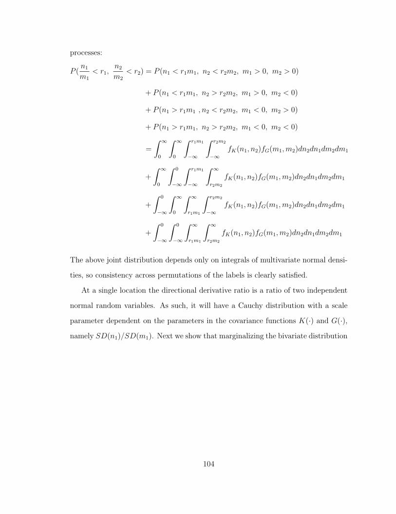
processes:

P (n1

m1

< r1,n2

m2

< r2) = P (n1 < r1m1, n2 < r2m2, m1 > 0, m2 > 0)

+ P (n1 < r1m1, n2 > r2m2, m1 > 0, m2 < 0)

+ P (n1 > r1m1 , n2 < r2m2, m1 < 0, m2 > 0)

+ P (n1 > r1m1, n2 > r2m2, m1 < 0, m2 < 0)

=

∫ ∞0

∫ ∞0

∫ r1m1

−∞

∫ r2m2

−∞fK(n1, n2)fG(m1,m2)dn2dn1dm2dm1

+

∫ ∞0

∫ 0

−∞

∫ r1m1

−∞

∫ ∞r2m2

fK(n1, n2)fG(m1,m2)dn2dn1dm2dm1

+

∫ 0

−∞

∫ ∞0

∫ ∞r1m1

∫ r2m2

−∞fK(n1, n2)fG(m1,m2)dn2dn1dm2dm1

+

∫ 0

−∞

∫ 0

−∞

∫ ∞r1m1

∫ ∞r2m2

fK(n1, n2)fG(m1,m2)dn2dn1dm2dm1

The above joint distribution depends only on integrals of multivariate normal densi-

ties, so consistency across permutations of the labels is clearly satisfied.

At a single location the directional derivative ratio is a ratio of two independent

normal random variables. As such, it will have a Cauchy distribution with a scale

parameter dependent on the parameters in the covariance functions K(·) and G(·),

namely SD(n1)/SD(m1). Next we show that marginalizing the bivariate distribution

104

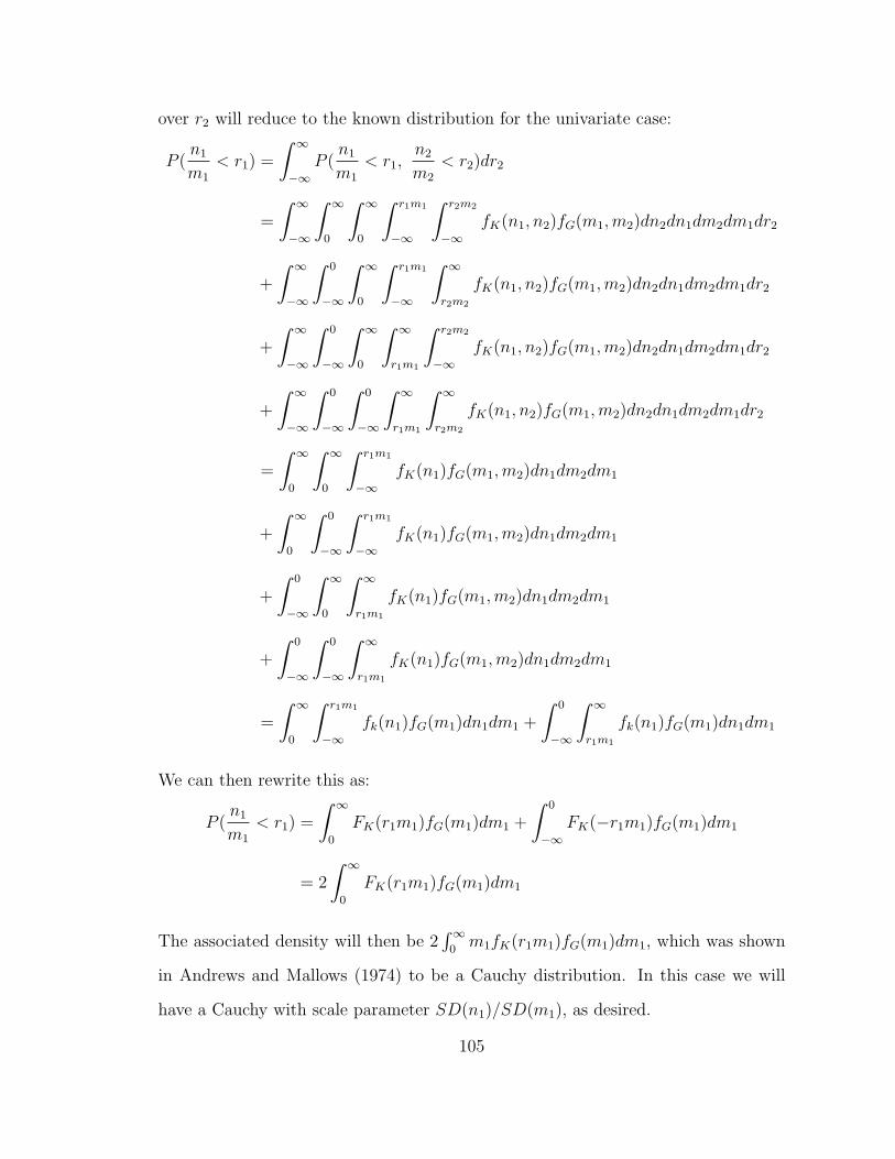
over r2 will reduce to the known distribution for the univariate case:

P (n1

m1

< r1) =

∫ ∞−∞

P (n1

m1

< r1,n2

m2

< r2)dr2

=

∫ ∞−∞

∫ ∞0

∫ ∞0

∫ r1m1

−∞

∫ r2m2

−∞fK(n1, n2)fG(m1,m2)dn2dn1dm2dm1dr2

+

∫ ∞−∞

∫ 0

−∞

∫ ∞0

∫ r1m1

−∞

∫ ∞r2m2

fK(n1, n2)fG(m1,m2)dn2dn1dm2dm1dr2

+

∫ ∞−∞

∫ 0

−∞

∫ ∞0

∫ ∞r1m1

∫ r2m2

−∞fK(n1, n2)fG(m1,m2)dn2dn1dm2dm1dr2

+

∫ ∞−∞

∫ 0

−∞

∫ 0

−∞

∫ ∞r1m1

∫ ∞r2m2

fK(n1, n2)fG(m1,m2)dn2dn1dm2dm1dr2

=

∫ ∞0

∫ ∞0

∫ r1m1

−∞fK(n1)fG(m1,m2)dn1dm2dm1

+

∫ ∞0

∫ 0

−∞

∫ r1m1

−∞fK(n1)fG(m1,m2)dn1dm2dm1

+

∫ 0

−∞

∫ ∞0

∫ ∞r1m1

fK(n1)fG(m1,m2)dn1dm2dm1

+

∫ 0

−∞

∫ 0

−∞

∫ ∞r1m1

fK(n1)fG(m1,m2)dn1dm2dm1

=

∫ ∞0

∫ r1m1

−∞fk(n1)fG(m1)dn1dm1 +

∫ 0

−∞

∫ ∞r1m1

fk(n1)fG(m1)dn1dm1

We can then rewrite this as:

P (n1

m1

< r1) =

∫ ∞0

FK(r1m1)fG(m1)dm1 +

∫ 0

−∞FK(−r1m1)fG(m1)dm1

= 2

∫ ∞0

FK(r1m1)fG(m1)dm1

The associated density will then be 2∫∞

0m1fK(r1m1)fG(m1)dm1, which was shown

in Andrews and Mallows (1974) to be a Cauchy distribution. In this case we will

have a Cauchy with scale parameter SD(n1)/SD(m1), as desired.

105

The marginalization is straight forward for larger dimensions with marginalization

over the two normal densities occurring in a similar way.

A.2 Bivariate Angular Density

We are interested in the marginal behavior of f(θX(s), θY (s)) at a location s where

tan(θX(s)) = D(0,1)X(s)/D(1,0)X(s), tan(θY (s)) = D(0,1)Y (s)/D(1,0)Y (s), and

(∇X(s),∇Y (s))′ = (D(1,0)Y (s), D(0,1)Y (s), D(1,0)X(s), D(0,1)X(s))′ are normally dis-

tributed with the covariance structure provided in Equation 1.

After converting to polar coordinates, the change of variables formula gives the

following integral, where g(·) is the multivariate normal density associated with

(∇Y (s),∇X(s))′. For clarity we suppress the index (s):

f(θX , θY ) =

∫ ∞0

∫ ∞0

g(ry cos θY , ry sin θY , rx cos θX , rx sin θX)ryrxdrydrx

=

∫ ∞0

rx1√

(2π)3|Σ|exp(−1

2(ac− A2)r2

x)

×(∫ ∞

0

ry

√a√

2πexp(−a

2(ry − βrx cos θ)2)dry

)drx

=1√

(2π)2|Σ|

×∫ ∞

0

1√2π

(Φ(Arx)Arx/

√a√

a+φ(Arx)

a

)rx exp(−1

2(ac− A2)r2

x)drx

=1√

(2π)2|Σ|

( 1√2πa

A√a

∫ ∞0

rxΦ(Arx)rx exp(−1

2(ac− A2)r2

x)drx

+

∫ ∞0

rx1

a√

2πφ(Arx) exp(−1

2(ac− A2)r2

x)drx

)

106

=

d

(1√2πa

A√a

(φ(0)A

ac(ac−A2)+

√2π

(ac−A2)3/2L(0, 0,√

A2

ac)

)+ φ(0)

a2c√

2π

), if A > 0

d

(1√2πa

A√a

(φ(0)A

ac(ac−A2)+

√2π

(ac−A2)3/2 (0.5− L(0, 0,√

A2

ac))

)+ φ(0)

a2c√

2π

), if A < 0

where d = 1√(2π)2|Σ|

, |Σ| = (σ2xφ

2x)

2(σ2yφ

2y)

2, a = 1/(σ2yφ

2y), c = (σ2

yφ2y+β

2φ2xσ

2x)/(σ

2xφ

2x),

A =√aβ cos(θX−θY ), and L(0, 0, ρ) is the zero mean bivariate normal cdf with cor-

relation ρ and standard deviations equal to 1 evaluated at (0, 0)′.

Several integration steps were treated as the expected value of a truncated normal

distribution. An additional integration step required integration by three parts, then

computation of the probability that the sum of a normal and a truncated normal are

less than some constant. This probability was available in closed form in the query

by Lipow et al. (1964) and is written in terms of the bivariate normal cdf. Somewhat

simplified, this gives the density provided in the text:

f(θX , θY ) =

C

(A2φ(0)

ac(ac−A2)+

√2πA

(ac−A2)3/2L(0, 0,√

A2

ac) + φ(0)

ac

), if A > 0

C

(A2φ(0)

ac(ac−A2)+

√2πA

(ac−A2)3/2

(0.5− L(0, 0,

√A2

ac)

)+ φ(0)

ac

), if A < 0

where C = 1

a(2π)3/2√|Σ|

.

107

Bibliography

Albert, J. H. and Chib, S. (1993), “Bayesian analysis of binary and polychotomousresponse data,” Journal of the American Statistical Association, 88, 669–679.

Andrews, D. F. and Mallows, C. L. (1974), “Scale mixtures of normal distributions,”Journal of the Royal Statistical Society. Series B (Methodological), pp. 99–102.

Banerjee, S. and Gelfand, A. (2003), “On smoothness properties of spatial processes,”Journal of Multivariate Analysis, 84, 85–100.

Banerjee, S. and Gelfand, A. E. (2006), “Bayesian wombling: Curvilinear gradi-ent assessment under spatial process models,” Journal of the American StatisticalAssociation, 101, 1487–1501.

Banerjee, S., Gelfand, A. E., and Sirmans, C. (2003), “Directional rates of changeunder spatial process models,” Journal of the American Statistical Association,98, 946–954.

Banerjee, S., Gelfand, A. E., and Carlin, B. P. (2004), Hierarchical modeling andanalysis for spatial data, CRC Press.

Banerjee, S., Gelfand, A. E., Finley, A. O., and Sang, H. (2008), “Gaussian predictiveprocess models for large spatial data sets,” Journal of the Royal Statistical Society:Series B (Statistical Methodology), 70, 825–848.

Baribault, T. W., Kobe, R. K., and Finley, A. O. (2012), “Tropical tree growth iscorrelated with soil phosphorus, potassium, and calcium, though not for legumes,”Ecological Monographs, 82, 189–203.

Berrett, C. and Calder, C. A. (2012), “Data augmentation strategies for the Bayesianspatial probit regression model,” Computational Statistics & Data Analysis, 56,478–490.

Canham, C. D. and Thomas, R. Q. (2010), “Frequency, not relative abundance, oftemperate tree species varies along climate gradients in eastern North America,”Ecology, 91, 3433–3440.

108

Clark, J. S. (2005), “Why environmental scientists are becoming Bayesians,” Ecologyletters, 8, 2–14.

Clark, J. S. and Gelfand, A. E. (2006), “A future for models and data in environ-mental science,” Trends in Ecology & Evolution, 21, 375–380.

Cressie, N. and Wikle, C. K. (2011), Statistics for spatio-temporal data, John Wiley& Sons.

Cressie, N., Calder, C. A., Clark, J. S., Hoef, J. M. V., and Wikle, C. K. (2009),“Accounting for uncertainty in ecological analysis: the strengths and limitationsof hierarchical statistical modeling,” Ecological Applications, 19, 553–570.

Finley, A. O., Banerjee, S., and Carlin, B. P. (2007), “spBayes: an R package forunivariate and multivariate hierarchical point-referenced spatial models,” Journalof Statistical Software, 19, 1.

Finley, A. O., Sang, H., Banerjee, S., and Gelfand, A. E. (2009), “Improving theperformance of predictive process modeling for large datasets,” Computationalstatistics & data analysis, 53, 2873–2884.

Fotheringham, A. S., Brunsdon, C., and Charlton, M. (2002), Geographicallyweighted regression, Wiley New York.

Fuentes, M. (2007), “Approximate likelihood for large irregularly spaced spatialdata,” Journal of the American Statistical Association, 102, 321–331.

Gelfand, A. E., Kim, H.-J., Sirmans, C., and Banerjee, S. (2003), “Spatial modelingwith spatially varying coefficient processes,” Journal of the American StatisticalAssociation, 98, 387–396.

Gelfand, A. E., Banerjee, S., and Gamerman, D. (2005), “Spatial process modellingfor univariate and multivariate dynamic spatial data,” Environmetrics, 16, 465–479.

Gelfand, A. E., Silander, J. A., Wu, S., Latimer, A., Lewis, P. O., Rebelo, A. G., andHolder, M. (2006), “Explaining species distribution patterns through hierarchicalmodeling,” Bayesian Analysis, 1, 41–92.

Gotway, C. A. and Young, L. J. (2002), “Combining incompatible spatial data,”Journal of the American Statistical Association, 97, 632–648.

Gryparis, A., Paciorek, C. J., Zeka, A., Schwartz, J., and Coull, B. A. (2009), “Mea-surement error caused by spatial misalignment in environmental epidemiology,”Biostatistics, 10, 258–274.

109

Guindani, M. and Gelfand, A. E. (2006), “Smoothness properties and gradient analy-sis under spatial Dirichlet process models,” Methodology and Computing in AppliedProbability, 8, 159–189.

Heagerty, P. J. and Lele, S. R. (1998), “A composite likelihood approach to binaryspatial data,” Journal of the American Statistical Association, 93, 1099–1111.

Higdon, D. (2002), “Space and space-time modeling using process convolutions,” inQuantitative methods for current environmental issues, pp. 37–56, Springer.

Jammalamadaka, S. R. and Sengupta, A. (2001), Topics in circular statistics, vol. 5,World Scientific.

Kent, J. T. (1989), “Continuity properties for random fields,” The Annals of Proba-bility, 17, 1432–1440.

Kim, H.-M., Mallick, B. K., and Holmes, C. (2005), “Analyzing nonstationary spa-tial data using piecewise Gaussian processes,” Journal of the American StatisticalAssociation, 100, 653–668.

Konomi, B. A., Sang, H., and Mallick, B. K. (2013), “Adaptive Bayesian nonstation-ary modeling for large spatial datasets using covariance approximations,” Journalof Computational and Graphical Statistics.

Lamont, B. B., Groom, P. K., and Cowling, R. (2002), “High leaf mass per area ofrelated species assemblages may reflect low rainfall and carbon isotope discrimina-tion rather than low phosphorus and nitrogen concentrations,” Functional Ecology,16, 403–412.

Lipow, M., Mantel, N., and Wilkinson, J. (1964), “Query 2: The Sum of Values froma Normal and a Truncated Normal Distribution (Continued),” Technometrics, 6,469–471.

Majumdar, A., Munneke, H. J., Gelfand, A. E., Banerjee, S., and Sirmans, C. (2006),“Gradients in spatial response surfaces with application to urban land values,”Journal of Business & Economic Statistics, 24.

Møller, J., Syversveen, A. R., and Waagepetersen, R. P. (1998), “Log gaussian coxprocesses,” Scandinavian Journal of Statistics, 25, 451–482.

Mugglin, A. S., Carlin, B. P., and Gelfand, A. E. (2000), “Fully model-based ap-proaches for spatially misaligned data,” Journal of the American Statistical Asso-ciation, 95, 877–887.

Murray, I. and Adams, R. P. (2010), “Slice sampling covariance hyperparameters oflatent Gaussian models,” arXiv preprint arXiv:1006.0868.

110

Murray, I., Adams, R. P., and MacKay, D. J. (2009), “Elliptical slice sampling,”arXiv preprint arXiv:1001.0175.

Paciorek, C. J. (2007), “Computational techniques for spatial logistic regression withlarge data sets,” Computational statistics & data analysis, 51, 3631–3653.

Peng, R. D. and Bell, M. L. (2010), “Spatial misalignment in time series studies ofair pollution and health data,” Biostatistics, 11, 720–740.

Poorter, H., Niinemets, U., Poorter, L., Wright, I. J., and Villar, R. (2009), “Causesand consequences of variation in leaf mass per area (LMA): a meta-analysis,” NewPhytologist, 182, 565–588.

Quick, H., Banerjee, S., Carlin, B. P., et al. (2013), “Modeling temporal gradientsin regionally aggregated California asthma hospitalization data,” The Annals ofApplied Statistics, 7, 154–176.

Rebelo, A. (2002), “The Protea Atlas Project,” Technical report. Accessed: 2002-05-12, http://protea.worldonline.co.za/default.htm.

Reich, B. J., Fuentes, M., and Dunson, D. B. (2011a), “Bayesian spatial quantileregression,” Journal of the American Statistical Association, 106.

Reich, B. J., Eidsvik, J., Guindani, M., Nail, A. J., Schmidt, A. M., et al. (2011b), “Aclass of covariate-dependent spatiotemporal covariance functions for the analysisof daily ozone concentration,” The Annals of Applied Statistics, 5, 2425–2447.

Royle, J. A. and Berliner, L. M. (1999), “A hierarchical approach to multivariatespatial modeling and prediction,” Journal of Agricultural, Biological, and Envi-ronmental Statistics, pp. 29–56.

Royle, J. A., Chandler, R. B., Gazenski, K. D., and Graves, T. A. (2013), “Spatialcapture-recapture models for jointly estimating population density and landscapeconnectivity,” Ecology, 94, 287–294.

Schultze, R. (1997), “South African Atlas of Agrohyrdology and Climatology.”Technical report, Report TT82/96, Water Research Commission, Pretoria, SouthAfrica.

Stein, M. L. (1999), Interpolation of spatial data: some theory for kriging, Springer.

Stein, M. L. (2013), “Limitations on low rank approximations for covariance matricesof spatial data,” Spatial Statistics.

Takhtajan, A., Crovello, T. J., and Cronquist, A. (1986), Floristic regions of theworld, University of California press Berkeley.

111

http://protea.worldonline.co.za/default.htm

Thomas, C. D. (2010), “Climate, climate change and range boundaries,” Diversityand Distributions, 16, 488–495.

Thuiller, W., Lavorel, S., Midgley, G., Lavergne, S., and Rebelo, T. (2004), “Relatingplant traits and species distributions along bioclimatic gradients for 88 Leucaden-dron taxa,” Ecology, 85, 1688–1699.

Tomovic, R. and Vukobratovic, M. (1972), General Sensitivity Theory. Number 35 inModern analytic and computational methods in science and mathematics, Elsevier,New York.

Ver Hoef, J. M., Cressie, N., and Barry, R. P. (2004), “Flexible spatial modelsfor kriging and cokriging using moving averages and the Fast Fourier Transform(FFT),” Journal of Computational and Graphical Statistics, 13, 265–282.

Wang, F. (2013), “Space and Space-Time Modeling of Directional Data,” PhD dis-sertation, Duke University.

Wheeler, D. C. and Calder, C. A. (2007), “An assessment of coefficient accuracy inlinear regression models with spatially varying coefficients,” Journal of Geograph-ical Systems, 9, 145–166.

Wheeler, D. C. and Waller, L. A. (2009), “Comparing spatially varying coefficientmodels: a case study examining violent crime rates and their relationships toalcohol outlets and illegal drug arrests,” Journal of Geographical Systems, 11, 1–22.

Wikle, C. K. and Cressie, N. (1999), “A dimension-reduced approach to space-timeKalman filtering,” Biometrika, 86, 815–829.

Wikle, C. K., Berliner, L. M., and Cressie, N. (1998), “Hierarchical Bayesian space-time models,” Environmental and Ecological Statistics, 5, 117–154.

112

Biography

Maria Antonia Terres was born in Nashua, N.H. on April 24, 1988. She graduated

with a Bachelor of Arts in Biology and Mathematics from Bard College at Simon’s

Rock in 2008 and a Master of Arts in Statistics from Columbia University in 2010.

In 2012 she earned a Master of Science in Statistical Science en route to the Ph.D.

She graduated with a Doctor of Philosophy under the supervision of Prof. Alan

Gelfand in 2014 from Duke University. As a graduate student at Duke she was

awarded the James B. Duke Fellowship and the 2014 Dean’s Award for Excellence

in Teaching. After completion of her Ph.D., she will be joining the Department of

Statistics at North Carolina State University as a postdoctoral research scholar under

the supervision of Prof. Montserrat Fuentes.

113

Documents

Multivariate Spatial Process Gradients with Environmental