Embed Size (px)
Citation preview

Multivariate ρ-Quantiles: a Spatial Approach∗
DIMITRI KONEN† and DAVY PAINDAVEINE‡
†,‡Universite libre de Bruxelles
ECARES and Departement de Mathematique
Avenue F.D. Roosevelt, 50
ECARES, CP114/04
B-1050, Brussels
Belgium
‡Universite Toulouse Capitole
Toulouse School of Economics
1, Esplanade de l’Universite
31080 Toulouse Cedex 06
France
By substituting an Lp loss function for the L1 loss function in the optimization problem
defining quantiles, one obtains Lp-quantiles that, as shown recently, dominate their classical
L1-counterparts in financial risk assessment. In this work, we introduce a concept of multivari-
ate Lp-quantiles generalizing the spatial (L1-)quantiles from Chaudhuri (1996). Rather than
restricting to power loss functions, we actually allow for a large class of convex loss functions ρ.
We carefully study existence and uniqueness of the resulting ρ-quantiles, both for a general prob-
ability measure over Rd and for a spherically symmetric one. Interestingly, the results crucially
depend on ρ and on the nature of the underlying probability measure. Building on an investiga-
tion of the differentiability properties of the objective function defining ρ-quantiles, we introduce
a companion concept of spatial ρ-depth, that generalizes the spatial depth from Vardi and Zhang
(2000). We study extreme ρ-quantiles and show in particular that extreme Lp-quantiles behave
in fundamentally different ways for p ≤ 2 and p > 2. Finally, we establish Bahadur represen-
tation results for sample ρ-quantiles and derive their asymptotic distributions. Throughout, we
impose only very mild assumptions on the underlying probability measure, and in particular we
never assume absolute continuity with respect to the Lebesgue measure.
MSC 2010 subject classifications: Primary 62G99, 62H99; secondary 62E20.
Keywords: Bahadur representation results, Convex objective functions, M-estimation, Multivari-
ate quantiles, Spatial depth, Spatial quantiles.
∗Research is supported by the Program of Concerted Research Actions (ARC) of the Universite
libre de Bruxelles and by an Aspirant fellowship from the FNRS (Fonds National pour la Recherche
Scientifique), Communaute Francaise de Belgique.
1
2 D. Konen and D. Paindaveine
1. Introduction
The concept of quantile, which is of paramount importance in statistics, has long been
limited to probability measures over R. Defining a suitable quantile concept in Rd is a
problem that is intrinsically difficult due to the lack of a canonical ordering in Rd, d > 1.
This has been an active research topic in the last decades; see, among many others, Hallin
et al. (2021), Hallin, Paindaveine and Siman (2010), Serfling (2002), and the references
therein. One of the most successful multivariate quantile concepts is the concept of spatial
(or geometric) quantiles from Chaudhuri (1996); for a probability measure P over Rd,the spatial quantile of order α in direction u is defined as the minimizer over Rd of the
map
µ 7→Mα,u(µ) =
∫Rd
{‖z − µ‖ − ‖z‖ − αu′µ
}dP (z), (1)
with α ∈ [0, 1) and u ∈ Sd−1 := {z ∈ Rd : ‖z‖2 := z′z = 1}. The success of spa-
tial quantiles is explained by several key distinctive properties, among which: spatial
quantiles are easy to compute, even for large d (Mukhopadhyaya and Chatterjee (2011),
Vardi and Zhang (2000)). The asymptotic behavior of their sample version is rather
standard (Chaudhuri (1996), Zhou and Serfling (2008)). They can easily be extended
into regression quantiles (Chakraborty (2003), Cheng and De Gooijer (2007)) or turned
into quantiles for functional data (Chakraborty and Chaudhuri (2014), Chowdhury and
Chaudhuri (2019), Serfling and Wijesuriya (2017)).
For d = 1, spatial quantiles, that minimize the L1-objective function in (1), reduce
to the usual univariate quantiles. In particular, the collection of intervals whose end-
points are the spatial quantiles of order α in direction u = −1 and u = 1 is a nested
family of interquantile intervals, that all contain the univariate median (which is ob-
tained with α = 0, irrespective of the direction u). Similarly, expectiles, an L2-analog of
quantiles introduced in Newey and Powell (1987), provide a nested family of centrality
intervals that all contain the mean of the distribution. Expectiles have met a big success,
particularly so in financial risk assessment, where they provide coherent risk measures;
see, e.g., Daouia, Girard and Stupfler (2018), Kuan, Yeh and Hsu (2009), Taylor (2008).
Quantiles and expectiles belong to the class of Lp-quantiles (associated with Lp loss func-
tions, with p ≥ 1), or, more generally, of M-quantiles (associated with general convex
loss functions); see Breckling and Chambers (1988), Chen (1996). Recently, there has
been a growing interest in such generalized quantiles, still with risk assessment as one of
the main applications; see, e.g., Daouia, Girard and Stupfler (2019), Gardes, Girard and
Stupfler (2020), or Usseglio-Carleve (2018).
The success of spatial quantiles in Rd and the growing interest in Lp-quantiles in the
univariate case d = 1 suggest to define a spatial concept of Lp-quantiles. For p = 2,
this has actually recently been done in Herrmann, Hofert and Mailhot (2018), but the
resulting spatial expectiles remain less well understood than their spatial L1-counterparts
from Chaudhuri (1996). To the best of our knowledge, a spatial Lp-quantile concept, or,

Multivariate ρ-Quantiles 3
more generally, a spatial M-quantile concept has not been investigated in the literature.
In this work, we define such a general concept and we thoroughly study its properties.
We adopt the following definition.
Definition 1. Let ρ : R+ → R+ be a convex function and P be a probability measure
over Rd. Fix α ∈ [0, 1) and u ∈ Sd−1. We say that µρα,u = µρα,u(P ) is a spatial ρ-quantile
of order α in direction u for P if and only if it minimizes the objective function
µ 7→Mρα,u(µ) :=
∫Rd
{Hρα,u(z − µ)−Hρ
α,u(z)}dP (z) (2)
over Rd, where we let
Hρα,u(z) := ρ(‖z‖)
(1 + α
u′z
‖z‖
)ξz,0, (3)
with ξz1,z2 := I[z1 6= z2] (throughout, I[A] is the indicator function of A).
It might have been natural to write µρv, with v = αu rather than µρα,u, to emphasize
the indexation of spatial ρ-quantiles on the unit ball, but we favour the notation µρα,uthat stresses the heterogenous roles α and u will play in the sequel. The multivariate Lp-
quantiles we consider in this work are obtained with ρ(t) = tp, p ≥ 1. Clearly, these
reduce for p = 1 to the minimizers of (1), that is, to the spatial quantiles from Chaudhuri
(1996). If P has finite second-order moments, then our Lp-quantiles reduce for p = 2 to
the expectiles introduced in Herrmann, Hofert and Mailhot (2018); as we will show,
however, our formulation above only requires that P has finite first-order moments. Note
that for α = 0, the ρ-quantile µρα,u, irrespective of u (the direction u does not play any
role for α = 0), is an M-functional of location, that, for p = 1 and p = 2, provides
the celebrated spatial median (Brown (1983)) and the mean vector of P , respectively.
The ρ-quantiles from Definition 1 extend this M-functional of location in the same way
the spatial quantiles from Chaudhuri (1996) extend the spatial median: they are thus
M-quantiles, in the sense of Breckling and Chambers (1988) or Koltchinski (1997) (it
should be noted that the only intersection between the M-quantiles in Definition 1 and
those from Koltchinski (1997) are the spatial quantiles from Chaudhuri (1996)).
Above, the motivation to consider Lp-quantiles was linked to their relevance for risk
assessment, and there is no doubt that spatial Lp-quantiles are natural tools to define
suitable risk measures in situations where multidimensional portfolios are considered.
The main focus in this work, however, is on a careful study of the probabilistic prop-
erties of these Lp-quantiles and, more generally, of the corresponding ρ-quantiles. Quite
remarkably, many of these properties crucially depend on the loss function ρ. We pro-
vide two examples. (i) Convexity of the objective function in (2) for any order α and
direction u is a key property for the study of ρ-quantiles and for their evaluation at
empirical distributions, and it may be expected that this convexity is inherited from the
convexity of ρ. Our results, however, will show that, in the class of Lp-quantiles, this is

4 D. Konen and D. Paindaveine
the case if and only if p ≤ 2. For p > 2, we will show that convexity holds for α ≤ αponly, where, quite remarkably, αp is very close to one for any p but does not depend
on p monotonically. (ii) The spatial quantiles from Chaudhuri (1996) have recently been
criticised because they exit any compact set as α→ 1 even for a compactly supported
probability measure P ; see Girard and Stupfler (2017). As our results will show, this
behavior of extreme spatial quantiles is shared by Lp-quantiles with p ≤ 2, but not by
those with p > 2. While we discussed these results here for Lp-quantiles only, we will
throughout study properties of ρ-quantiles for a virtually arbitrary convex loss function ρ,
which will allow us to consider, e.g., exponential loss functions or the celebrated Huber
loss functions.
The outline of the paper is as follows. In Section 2, we provide the assumptions under
which the objective function Mρα,u(µ) in (2) is well-defined for any µ, and we discuss
existence of ρ-quantiles. In Section 3, we obtain a necessary and sufficient condition for
convexity of Mρα,u(µ), we characterize the orders α for which convexity fails when this
condition is not satisfied, and we exploit this to derive uniqueness results for ρ-quantiles.
In Section 4, we refine these convexity and uniqueness results in the particular case
for which the underlying probability measure is spherically symmetric. In Section 5, we
study first- and second-order differentiability of the objective function Mρα,u(µ), which
will play a key role in the subsequent sections. In Section 6, we exploit Robert Serfling’s
DOQR paradigm to define ρ-depth functions, ρ-outlyingness functions and ρ-rank func-
tions associated with our ρ-quantile functions. We also identify conditions under which
ρ-quantile functions are homeomorphisms from the open unit ball (quantiles are indexed
by (α, u) ∈ [0, 1)×Sd−1 or, equivalently, by αu in the open unit ball of Rd) to the whole
Euclidean space Rd. This will play a major role when studying in Section 7 the behavior
of extreme ρ-quantiles. In Section 8, we derive Bahadur representation results for sample
ρ-quantiles and deduce their asymptotic distribution. Finally, we briefly discuss some
perspectives for future research in Section 9. Proofs are collected in the Supplementary
Material (Konen and Paindaveine (2021)).
2. Existence
Throughout, we assume that the loss function ρ belongs to the class C of functions
from R+ to R+ that are convex, piecewise twice continuously differentiable on (0,∞),
and satisfy ρ(t) = 0 only for t = 0. Here, ρ is piecewise twice continuously differentiable
on (0,∞) means that either (i) there exist a nonnegative integer K and (0 =: t0 <)t1 <
t2 < . . . < tK < tK+1 := ∞ such that ρ is twice continuously differentiable on each
open interval (tk, tk+1), k = 0, . . . ,K, or (ii) there exists a monotone strictly increasing
sequence (t0 := 0, t1, t2, . . .) in R+ diverging to infinity such that ρ is twice continuously
differentiable on each open interval (tk, tk+1), k ∈ N. We let Dρ = (0,∞)\{t1, t2, . . . , tK}in case (i) and Dρ = (0,∞)\{t1, t2, . . .} in case (ii). Examples of loss functions in C are the

Multivariate ρ-Quantiles 5
power loss functions ρ(t) = tp, with p ≥ 1, the exponential functions ρ(t) = exp(ct)− 1,
with c > 0, and the Huber loss functions ρ(t) = (t2/2)I[0 < t < c] + c(t− (c/2))I[t ≥ c],
with c > 0. For the Huber loss functions, Dρ = (0,∞) \ {c}, whereas Dρ = (0,∞) for
power and exponential loss functions.
For any ρ ∈ C, we denote as Pρd the class of probability measures P over Rd such that
for any µ ∈ Rd, there exists δ > 0 for which∫Rdψ−(‖z − µ‖+ δ) dP (z) <∞; (4)
throughout, ψ− and ψ+ will denote the left- and right-derivative of ρ, respectively (con-
vexity of ρ ensures existence of these one-sided derivatives). For the power loss func-
tion ρ(t) = tp, with p ≥ 1, P ∈ Pρd if and only if P has finite moments of order p−1 (that
is, E[‖Z‖p−1] < ∞, where Z is a random d-vector with distribution P ). For ρ(t) = t,
Pρd thus collects all probability measures on Rd, which is also the case for Huber loss
functions.
We then have the following existence result (see Section S.2 in Konen and Paindaveine
(2021) for a proof).
Theorem 2.1. Let ρ ∈ C and P ∈ Pρd . Fix α ∈ [0, 1] and u ∈ Sd−1. Then,
(i) Mρα,u(µ) is well-defined for any µ ∈ Rd; (ii) if α < 1, then P admits at least one
ρ-quantile of order α in direction u.
The existence result in Theorem 2.1(ii) is obtained by establishing that, for any α ∈[0, 1) and u ∈ Sd−1, the map µ 7→ Mρ
α,u(µ) is both coercive (in the sense that Mρα,u(µ)
diverges to infinity as ‖µ‖ does) and continuous on Rd. We require that ρ ∈ C in Theo-
rem 2.1 to avoid introducing many different collections of loss functions in the sequel, but
inspection of the proof reveals that the result actually holds without any differentiability
assumption on ρ.
Theorem 2.1(ii) shows that, for ρ(t) = tp, with p ≥ 1, ρ-quantiles exist for any α ∈ [0, 1)
and u ∈ Sd−1 as soon as P has finite moments of order p−1 (while subtracting Hρα,u(z) in
the integrand of (2) in principle has no impact on the corresponding quantile minimizers,
not doing so would guarantee existence of a minimizer only under the stronger condition
of finite moments of order p). In particular, taking p = 1 and p = 2, this shows that the
quantiles from Chaudhuri (1996) always exist, whereas their expectile analogs from Her-
rmann, Hofert and Mailhot (2018) only require that P has finite first-order moments (as
already mentionned, finite second-order moments are imposed in Herrmann, Hofert and
Mailhot (2018)). The quantiles associated with Huber loss functions also always exist for
any α ∈ [0, 1) and u ∈ Sd−1.
In Section 7 below, we will study extreme ρ-quantiles, that is, the ρ-quantiles indexed
by an order α that is arbitrarily close to one. As we will see, the behavior of such
quantiles crucially depends on the existence of the boundary ρ-quantiles indexed by an
6 D. Konen and D. Paindaveine
order α = 1 (the term “boundary” results from the fact that Definition 1 imposes that α ∈[0, 1)). Our interest in such boundary quantiles explains why we will be investigating the
properties of the map Mρα,u(µ) also for α = 1, as we already did in Theorem 2.1(ii).
At this stage, we stress that Theorem 2.1(ii) remains silent about the existence of such
boundary ρ-quantiles, the reason being that coercivity of µ 7→Mρα,u(µ) may fail for α =
1. For ρ(t) = t and d ≥ 2, for instance, no such boundary quantiles exist when P
is non-atomic and is not supported on a line of Rd; see Girard and Stupfler (2017),
Proposition 2.1.
We conclude this section with the following orthogonal- and translation-equivariance
result, that will be particularly relevant in Section 4 when considering the particular case
for which P is spherically symmetric (the proof readily follows from Definition 1).
Proposition 2.1. Let ρ ∈ C and P ∈ Pdρ . Fix α ∈ [0, 1) and u ∈ Sd−1. Let O be a d×dorthogonal matrix, b be a d-vector, and denote as PO,b the distribution of OZ+ b when Z
has distribution P . Then, if µ is a ρ-quantile of P of order α in direction u, then Oµ+ b
is a ρ-quantile of PO,b of order α in direction Ou.
Spatial ρ-quantiles are not affine-equivariant, that is, they fail to be equivariant under
general affine transformations. However, they can be made affine-equivariant through a
transformation-retransformation approach; see, e.g., Serfling (2010) in the case of the
Chaudhuri (1996) spatial quantiles.
3. Convexity and uniqueness
The quantiles studied in this work are defined as minimizers of the map µ 7→ Mρα,u(µ)
in (2). Convexity of this map is a most desirable property, that is expected to play a
key role when investigating uniqueness of these quantiles and when evaluating them for
empirical probability measures. In this section, we therefore study under which conditions
on the loss function ρ ∈ C the map µ 7→Mρα,u(µ) is convex for any P ∈ Pρd .
First note that convexity of Hρα,u trivially implies convexity of Mρ
α,u, and that, if Hρα,u
is not convex, then there exists P ∈ Pρd for which Mρα,u fails to be convex (simply consider
a Dirac probability measure). Therefore, we may focus on studying convexity of Hρα,u.
Since any ρ ∈ C clearly makes Hρα,u convex for d = 1, we tacitly restrict throughout this
section to the case d ≥ 2. We start with the following preliminary result showing that
the larger α, the fewer the functions ρ making Hρα,u convex for any u ∈ Sd−1.
Lemma 3.1. For any α ∈ [0, 1], denote as Cα the collection of functions ρ ∈ C such
that Hρα,u is convex for any u ∈ Sd−1. Then, we have the following:
(i) C0 = C; (ii) if α1, α2 ∈ [0, 1] satisfy α1 < α2, then Cα2⊆ Cα1
.

Multivariate ρ-Quantiles 7
This result suggests considering αρ := max{α ∈ [0, 1] : ρ ∈ Cα}, the largest value of α
for which ρ makes Hρα,u convex for any u ∈ Sd−1 (it is trivial to prove that the maximum
exists for any ρ ∈ C). Ideally, we would like to have that αρ = 1, as this would ensure
that Hρα,u is convex for any α ∈ [0, 1] and u ∈ Sd−1. The following result provides a
necessary and sufficient condition for αρ = 1.
Theorem 3.1. Let ρ ∈ C. Then, irrespective of d ≥ 2, αρ = 1 if and only if the map
t 7→ t2/ρ(t) is concave on (0,∞).
As a corollary, the power loss function ρ(t) = tp makes Hρα,u convex for any α ∈ [0, 1)
and any u ∈ Sd−1 if and only if p ∈ [1, 2]. For p > 2, it is then of interest to determine
the corresponding value of αρ(< 1). More generally, the following result allows one to
determine αρ for any loss function ρ that does not satisfy the necessary and sufficient
condition in Theorem 3.1.
Theorem 3.2. Let ρ ∈ C be such that the map t 7→ t2/ρ(t) is not concave on (0,∞).
Then, irrespective of d ≥ 2,
αρ = inft∈Dcv
ρ
√qt(4p2t − 4pt − qt)4(pt − 1)2(qt + 1)
< 1,
with
pt :=tψ−(t)
ρ(t)and qt :=
t2ψ′−(t)
tψ−(t)− ρ(t),
where we let Dcvρ := {t ∈ Dρ : (t2/ρ(t))′′ > 0} and where ψ′− is the left-derivative of ψ−
(in this result, ψ−(t) and ψ′−(t) are used only for t ∈ Dρ, so that we could write ψ−(t) =
ρ′(t) and ψ′−(t) = ρ′′(t) above).
For ρ(t) = tp with p > 2, one readily checks that Dcvρ = (0,∞) and
αρ :=
√p2(4p− 5)
4(p− 1)2(p+ 1)· (5)
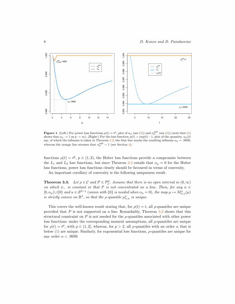
Remarkably, αρ in (5) exhibits a non-monotonic pattern in p: for p ∈ [2, 5], it decreases
monotonically from one to its minimal value√
125/128 (slightly above .9882), then
increases monotonically to one again for p ∈ [5,∞); see the left panel of Figure 1.
For p > 2, it is thus only for most extreme quantile orders α that convexity fails.
This is even more the case for the exponential loss function ρ(t) = exp(ct) − 1, for
which Dcvρ = (3.0861/c,∞) and αρ = .9939. It can be shown that, if the loss function ρ
is such that t 7→ ρ(t)/t is convex, then αρ ≥√
2/3 ≈ .8165 (for the sake of completeness,
we prove this in Konen and Paindaveine (2021); see Corollary S.3.1). Like the power loss
8 D. Konen and D. Paindaveine
2 4 6 8 10 12 14
0.985
0.990
0.995
1.000
p
α5=.9882
α2.429sph =.9987
αpsph
αp
5 10 15 20 25
0.993
0.994
0.995
0.996
0.997
0.998
0.999
1.000
t
αρsph=1
αρ=.9939
αρsph
αρ
αρ(t)
Figure 1. (Left:) For power loss functions ρ(t) = tp, plot of αρ (see (5)) and αsphρ (see (6)) (note that (5)
shows that αρ → 1 as p→∞). (Right:) For the loss function ρ(t) = exp(t)−1, plot of the quantity, αρ(t)say, of which the infimum is taken in Theorem 3.2; the blue line marks the resulting infimum αρ = .9939,
whereas the orange line stresses that αsphρ = 1 (see Section 4).
functions ρ(t) = tp, p ∈ (1, 2), the Huber loss functions provide a compromise between
the L1 and L2 loss functions, but since Theorem 3.2 entails that αρ = 0 for the Huber
loss functions, power loss functions clearly should be favoured in terms of convexity.
An important corollary of convexity is the following uniqueness result.
Theorem 3.3. Let ρ ∈ C and P ∈ Pdρ . Assume that there is no open interval in (0,∞)
on which ψ− is constant or that P is not concentrated on a line. Then, for any α ∈[0, αρ)∪{0} and u ∈ Sd−1 (union with {0} is needed when αρ = 0), the map µ 7→Mρ
α,u(µ)
is strictly convex on Rd, so that the ρ-quantile µρα,u is unique.
This covers the well-known result stating that, for ρ(t) = t, all ρ-quantiles are unique
provided that P is not supported on a line. Remarkably, Theorem 3.3 shows that this
structural constraint on P is not needed for the ρ-quantiles associated with other power
loss functions: under the corresponding moment assumptions, all ρ-quantiles are unique
for ρ(t) = tp, with p ∈ (1, 2], whereas, for p > 2, all ρ-quantiles with an order α that is
below (5) are unique. Similarly, for exponential loss functions, ρ-quantiles are unique for
any order α < .9939.

Multivariate ρ-Quantiles 9
4. The spherical case
In this section, we consider the special case for which P (∈ Pρd ) is spherically symmetric
about some location µ0(∈ Rd), in the sense that, for any d-Borel set B and any d× d or-
thogonal matrix O, the P -probability of µ0+OB does not depend on O. Since ρ-quantiles
are translation-equivariant, we will actually restrict, without any loss of generality, to the
case µ0 = 0 (translation-equivariance here means that if µ is a ρ-quantile of P of order α
in direction u, then, for any h ∈ Rd, µ+ h is a ρ-quantile of Ph of order α in direction u,
where Ph is the distribution of Z + h when Z has distribution P ).
Note that it follows from Proposition 2.1 that, if P is spherically symmetric about
the origin of Rd and satisfies P [{0}] < 1, with d ≥ 2 say, then any quantile contour
{µα,u : u ∈ Sd−1}, with α ∈ [0, αρ)∪{0}, is a hypersphere (uniqueness of these quantiles
follows from Theorem 3.3 since P is then not supported on a line). Proposition 2.1 then
also implies that, for an arbitrary order α ∈ [0, 1) and any direction u ∈ Sd−1, the ρ-
quantiles of P of order α in direction u form a set that is invariant under all rotations
fixing u. In particular, if µρα,u is unique, then it belongs to the line spanned by u, which
is most natural. For α ≥ αρ, however, uniqueness is not guaranteed, so that it is unclear
whether or not quantiles meet this natural property in the spherical case. This motivates
the following result.
Theorem 4.1. Let ρ ∈ C and P ∈ Pρd . Assume that P is spherically symmetric about
the origin of Rd. Then, (i) for α = 0 and any u ∈ Sd−1, the unique ρ-quantile µρα,u is
the origin of Rd; (ii) for α ∈ (0, 1) and u ∈ Sd−1, any ρ-quantile µρα,u belongs to the
halfline {λu : λ ≥ 0}.
In case (ii), the origin of Rd may be a ρ-quantile of order α > 0 in direction u. Actually,
it can be shown that (a) for ρ(t) = t, the origin is a ρ-quantile of order α > 0 in direction u
if and only α ≤ P [{0}]. Moreover, (b) provided that ψ+(0)P [{0}]+P [‖Z‖ ∈ (0,∞)\Dρ] =
0 where Z has distribution P (a condition that always holds for ρ(t) = tp with p > 1),
the origin cannot be a ρ-quantile of order α > 0 in direction u, so that all these quantiles
then belong to {λu : λ > 0} (for the sake of completeness, we prove (a)–(b) in Konen
and Paindaveine (2021); see Proposition S.4.1).
If P is spherically symmetric about the origin and satisfies P [{0}] < 1, Theorem 3.3
shows that ρ-quantiles are unique for any α < αρ (as mentioned above) but it remains
silent on the case α ≥ αρ. Interestingly, we will be able to say more under sphericity,
thanks to the fact that Theorem 4.1 entails that uniqueness will hold if t 7→Mρα,u(tu) is
strictly convex over [0,∞) for all u ∈ Sd−1, which in turn will hold if t 7→ Hρα,u(z − tu)
is convex for any z ∈ Rd and any u ∈ Sd−1. Accordingly, for any α ∈ [0, 1], let Csphα be
the collection of functions ρ ∈ C such that t 7→ Hρα,u(z − tu) is convex for any z ∈ Rd
and u ∈ Sd−1. Since Csph0 = C and Csphα2⊆ Csphα1
for any α1 < α2 (see the proof of
10 D. Konen and D. Paindaveine
Theorem 4.2 below), we let αsphρ := max{α ∈ [0, 1] : ρ ∈ Csphα }, parallel to what we did
for αρ in Section 3. We have the following result.
Theorem 4.2. Let ρ ∈ C and P ∈ Pρd . Assume that P is spherically symmetric about
the origin of Rd. Then, for any α ∈ [0, αsphρ ) ∪ {0} and u ∈ Sd−1 (again, union with {0}
is needed when αsphρ = 0), the map t 7→ Mρ
α,u(tu) is strictly convex on [0,∞), and the
ρ-quantile µρα,u is unique.
Note that, in the present spherical setup, this uniqueness result may only strengthen
the one in Theorem 3.3, since the fact that Cα ⊆ Csphα for any α ∈ [0, 1] implies that αsphρ ≥
αρ. Of course, it is natural to wonder under which conditions on ρ all ρ-quantiles are
unique (αsphρ = 1) and, when these conditions are not met, what are the orders α for
which uniqueness is guaranteed (that is, what is then the value of αsphρ < 1). The following
result provides a complete answer to these questions.
Theorem 4.3. Let ρ ∈ C. Then, (i) αsphρ = 1 if and only if 4pt + qt − ptqt ≤ 6 for
any t ∈ Dρ, where pt and qt are as in Theorem 3.2; (ii) if αsphρ < 1, then, letting Dsph
ρ :=
{t ∈ Dρ : 4pt + qt − ptqt > 6}(⊆ Dcvρ ),
αsphρ = inf
t∈Dsphρ
√βpt,qt ,
where
βp,q :=2(pq − p− q)3(
√cp,q − q(2p− 3)/3)2
3(p− 1)2(3− p)(√cp,q − (2p− q))(√cp,q − q(2p− 3))2
involves cp,q := q3 (3−2p)(2pq−8p+q) (if q makes βp,q undefined in the expression above,
then we let βp,q := limr→q βp,r).
Parallel to αρ in Theorems 3.1–3.2, αsphρ does not depend on d(≥ 2). For the power
loss functions ρ(t) = tp with p ≥ 1, it follows from Theorem 4.3 that
αsphρ =
√
p2(p−2)3(bp−(p− 32 )
2)
(p−1)2(3−p)(bp− 32 )(bp−3(p−
32 )
2)(<1) if p ∈ (2, 3)
1 otherwise,
(6)
with bp :=(3(p− 3
2 )( 72 − p)
)1/2. For p ∈ [1, 2], the result is just a corollary of Theorem 3.1
since we then have αsphρ ≥ αρ = 1. For p > 3, (6) implies that all ρ-quantiles are uniquely
defined under sphericity, while there is no guarantee that this is the case in general (since
αρ < 1 for such values of p). As shown in Figure 1, the values of αsphp for p ∈ (2, 3) are
remarkably close to one (the minimal value, achieved at p ≈ 2.429, is about .9987),
which implies that, also for p ∈ (2, 3), essentially all ρ-quantiles are uniquely defined
under sphericity. For the exponential loss functions ρ(t) = exp(ct)−1, all ρ-quantiles are
also unique under sphericity (αsphρ = 1), while “only” quantiles of order α < αρ = .9939
are guaranteed to be unique in general.
Multivariate ρ-Quantiles 11
5. Differentiability of the objective function
For any α < αρ, the ρ-quantiles µρα,u are minimizers of the convex objective function µ 7→Mρα,u(µ). If this objective function is smooth, then ρ-quantiles are characterized by the
first-order condition ∇Mρα,u(µρα,u) = 0. Such a gradient condition will actually play a key
role when deriving further properties of ρ-quantiles in the next sections. This provides
a strong motivation to study smoothness of the map µ 7→ Mρα,u(µ). We start with the
following result.
Proposition 5.1. Let ρ ∈ C and P ∈ Pρd . Fix α ∈ [0, 1] and u ∈ Sd−1. Let Z be a
random d-vector with distribution P and write Zµ := Z − µ, for any µ ∈ Rd. Then, for
any µ ∈ Rd and v ∈ Rd \ {0}, the directional derivative
∂Mρα,u
∂v(µ) = lim
t>→0
Mρα,u(µ+ tv)−Mρ
α,u(µ)
t
exists and is given by
∂Mρα,u
∂v(µ) = ψ+(0)(‖v‖ − αu′v)P [{µ}]− αv′E
[ρ(‖Zµ‖)‖Zµ‖
(Id −
ZµZ′µ
‖Zµ‖2
)ξZ,µ
]u
−v′E[{ψ−(‖Zµ‖)I[v′Zµ > 0] + ψ+(‖Zµ‖)I[v′Zµ < 0]}
(1 + α
u′Zµ‖Zµ‖
)Zµ‖Zµ‖
],
where Id is the d× d identity matrix and ξz1,z2 is as in Definition 1.
The objective function thus admits directional derivatives in all directions (hence, is
continuous over Rd), but it is not necessarily differentiable. For instance, the classical
spatial quantiles obtained with ρ(t) = t provide
∂Mρα,u
∂v(µ) = (‖v‖ − αu′v)P [{µ}] + v′E
[(µ− Z‖µ− Z‖
− αu)ξZ,µ
],
so that Mρα,u fails to be differentiable at atoms of P . Clearly, it follows from Theo-
rem 5.1 that a necessary condition for this objective function to be differentiable at µ
is ψ+(0)P [{µ}] = 0. The next result provides a necessary and sufficient condition and
gives an expression for the corresponding gradient.
Theorem 5.1. Let ρ ∈ C and P ∈ Pρd . Fix α ∈ [0, 1] and u ∈ Sd−1. Then,
(i) µ 7→Mρα,u(µ) is differentiable at µ0(∈ Rd) if and only if ψ+(0)P [{µ0}]+P [‖Z−µ0‖ ∈
(0,∞) \ Dρ] = 0, in which case the corresponding gradient is
∇Mρα,u(µ0) = v(µ0)− αT (µ0)u, with v(µ) := −E
[ψ−(‖Zµ‖)
Zµ‖Zµ‖
ξZ,µ
]

12 D. Konen and D. Paindaveine
and
T (µ) := E
[{ρ(‖Zµ‖)‖Zµ‖
(Id −
ZµZ′µ
‖Zµ‖2
)+ ψ−(‖Zµ‖)
ZµZ′µ
‖Zµ‖2
}ξZ,µ
],
where Zµ := Z − µ is based on a random d-vector Z with distribution P .
(ii) If ψ+(0)P [{µ}] + P [‖Z − µ‖ ∈ (0,∞) \ Dρ] = 0 for any µ in an open set N ,
then µ 7→Mρα,u(µ) is continuously differentiable on N .
It follows from this result that, in contrast with ρ(t) = t, the power loss functions ρ(t) =
tp with p > 1 make the objective function Mρα,u (continuously) differentiable even in the
atomic case. The corresponding quantiles µρα,u are thus the solutions of the first-order
equations ∇Mρα,u(µ) = 0, which rewrite
−pE[‖Zµ‖p−1
Zµ‖Zµ‖
ξZ,µ
]= αE
[‖Zµ‖p−1
(Id + (p− 1)
ZµZ′µ
‖Zµ‖2
)ξZ,µ
]u.
In particular, spatial expectiles (p = 2) of order α in direction u are the unique (Theo-
rem 3.3) solutions of
2(µ− E[Z]) = αE
[‖Z − µ‖
(Id +
(Z − µ)(Z − µ)′
‖Z − µ‖2ξZ,µ
)]u.
This is compatible with the fact that the corresponding “median” (that is, the quantile
of order α = 0, in an arbitrary direction u) is the mean vector E[Z].
We turn to second-order differentiability, which will be relevant when studying the
asymptotic behavior of sample ρ-quantiles in Section 8.
Theorem 5.2. Let ρ ∈ C and P ∈ Pρd . Fix α ∈ [0, 1], u ∈ Sd−1, and µ0 ∈ Rd. Assume
that P [‖Z − µ‖ ∈ [0,∞) \ Dρ] = 0 for any µ in an open neighbourhood of µ0 (hence, in
particular, that P is non-atomic in this neighbourhood). Let further one of the following
assumptions hold:
(A) ψ− is concave on (0,∞) and∫Rd\{µ0}
ψ−(‖z − µ0‖)‖z − µ0‖
dP (z) <∞;
(A′) ψ− is convex on (0,∞), ψ+(0) = 0, and there exists r > 0 such that∫Rdψ′−(‖z − µ0‖+ r) dP (z) <∞
(recall that ψ′− is the left-derivative of ψ−).

Multivariate ρ-Quantiles 13
Then, for any v ∈ Rd \ {0},
limt>→0
∇Mρα,u(µ0 + tv)−∇Mρ
α,u(µ0)
t= ∇2Mρ
α,u(µ0)v,
where the Hessian matrix ∇2Mρα,u(µ) is given by
∇2Mρα,u(µ) =
(∂i∂jM
ρα,u(µ)
)i,j=1,...,d
= E
[(ψ′−(‖Zµ‖)−
2ψ−(‖Zµ‖)‖Zµ‖
+2ρ(‖Zµ‖)‖Zµ‖2
)(1 + α
u′Zµ‖Zµ‖
)ZµZ
′µ
‖Zµ‖2ξZ,µ
+ρ(‖Zµ‖)‖Zµ‖2
(Id −
ZµZ′µ
‖Zµ‖2
)ξZ,µ +
‖Zµ‖ψ−(‖Zµ‖)− ρ(‖Zµ‖)‖Zµ‖2
×{(
1 + αu′Zµ‖Zµ‖
)(Id −
ZµZ′µ
‖Zµ‖2
)+ 2
ZµZ′µ
‖Zµ‖2+ α
Zµu′ + Z ′µu
‖Zµ‖
}ξZ,µ
](as in the previous results, Zµ := Z − µ, where Z is a random d-vector with distribu-
tion P ).
While they may seem complex at first, the assumptions of Theorem 5.2 turn out
to be simple (and very weak) when considering specific loss functions ρ. For instance,
for ρ(t) = tp with p ≥ 1, they only require that P ∈ Pρd is non-atomic in a neighborhood
of µ0 and is such that E[‖Z − µ0‖p−2] < ∞ when Z has distribution P . Note that this
last assumption, that cannot be avoided since this expectation is involved in the Hessian
matrix ∇2Mρα,u(µ), is superfluous for p ≥ 2. Under the assumptions of Theorems 3.3
and 5.2, this Hessian matrix is positive definite for any α ∈ [0, αρ)∪{0} and any u ∈ Sd−1;
since this will be needed in the sequel, we prove it in Konen and Paindaveine (2021) (see
Lemma S.8.2).
6. A ρ-version of Robert Serfling’s DOQR paradigm
In a series of papers, Robert Serfling introduced the DOQR paradigm, that presents
Depth, Outlyingness, Quantile and Rank functions as interrelated, yet distinct, objects
of interest for multivariate nonparametric statistics; see, e.g., Serfling (2010), Serfling
(2019), Serfling and Zuo (2010) and the references therein. While this paradigm in prin-
ciple applies to any multivariate quantile concept, the primary focus when considering
this paradigm in the aforementioned papers was on spatial quantiles. This makes it nat-
ural to study the paradigm for the generalized spatial quantiles considered in this work,
which leads to introducing ρ-depth, ρ-outlyingness, ρ-quantile and ρ-rank functions. As
we will see later, some of these functions play a key role to understand the nature of
extreme ρ-quantiles.
14 D. Konen and D. Paindaveine
We start by formally defining ρ-quantile functions. Restricting to the interesting case
for which αρ > 0, Theorems 2.1 and 3.3 imply that ρ-quantiles exist and are unique for
any α ∈ [0, αρ) and u ∈ Sd−1, which allows us to adopt the following definition.
Definition 2. Let ρ ∈ C and P ∈ Pdρ . Assume that there is no open interval in (0,∞)
on which ψ− is constant or that P is not concentrated on a line. Write Bdr = {z ∈ Rd :
‖z‖ < r}. Then, the ρ-quantile function of P is the map Q = QρP : Bdαρ → Rd that is
defined through Q(αu) = µρα,u.
In dimension d = 1 and ρ(t) = t, this provides the (centered-outward version of
the) usual quantile function. This standard quantile function, that is defined on B11 =
(−1, 1), may of course fail to be continuous (it is discontinuous for empirical probability
measures). The multivariate case d ≥ 2 is different.
Proposition 6.1. Let ρ ∈ C and P ∈ Pdρ , with d ≥ 2. Assume that there is no open
interval in (0,∞) on which ψ− is constant or that P is not concentrated on a line. Then,
the quantile function Q = QρP : Bdαρ → Rd is continuous.
Following Serfling (2010), we associate with the ρ-quantile function Q corresponding
concepts of rank function R, depth function D and outlyingness function O. We start
with the rank function.
Definition 3. Let ρ ∈ C and assume that P ∈ Pdρ is not a Dirac probability measure.
Then, the rank function of P is the map R = RρP : Rd → Rd defined through R(µ) =
(T (µ))−1v(µ), where the d × d matrix T (µ) and the d-vector v(µ) were introduced in
Theorem 5.1.
In the setup of this definition, T (µ) is positive definite, hence invertible, for any µ ∈Rd (for the sake of completeness, we prove this in Konen and Paindaveine (2021); see
Lemma S.6.1). The natural assumptions under which to study the rank function are those
of Theorem 5.1 complemented by conditions ensuring uniqueness of ρ-quantiles (which
provides the assumptions in Theorem 6.1 below). Under these assumptions, µ 7→Mρα,u(µ)
is continuously differentiable on Rd, with gradient
∇Mρα,u(µ) = T (µ)(R(µ)− αu),
so that µ = µα,u = Q(αu) (for α < αρ) if and only if R(µ) = αu (recall that, under the
assumptions considered, quantiles of order α ∈ [0, αρ) in direction u ∈ Sd−1 are indeed
uniquely determined by the gradient condition ∇Mρα,u(µ) = 0). This provides a clear
interpretation of the rank function as the inverse map of the quantile function. We have
the following result.

Multivariate ρ-Quantiles 15
Theorem 6.1. Let ρ ∈ C and P ∈ Pρd . Assume that there is no open interval in (0,∞)
on which ψ− is constant or that P is not concentrated on a line. Assume further that
ψ+(0)P [{µ}] + P [‖Z − µ‖ ∈ (0,∞) \ Dρ] = 0 for any µ ∈ Rd. Write Zρ = QρP (Bdαρ).Then, Q = QρP : Bdαρ → Zρ is a homeomorphism, with inverse RρP |Zρ : Zρ → Bdαρ (therestriction of RρP to Zρ).
If t 7→ t2/ρ(t) is concave on (0,∞), then we are in the important particular case αρ = 1
(Theorem 3.1), for which the quantile function Q is defined on the open unit ball Bd = Bd1 .
We then have the following result.
Theorem 6.2. Let ρ ∈ C be such that t 7→ t2/ρ(t) is concave on (0,∞). Assume that P
is not concentrated on a line and that ψ+(0)P [{µ}] + P [‖Z − µ‖ ∈ (0,∞) \ Dρ] = 0 for
any µ ∈ Rd. Then, Zρ = QρP (Bd) = Rd, so that Q = QρP : Bd → Rd is a homeomorphism,
with inverse R = RρP : Rd → Bd.
This result shows in particular that for any power loss function ρ(t) = tp with p ∈[1, 2], any non-atomic probability measure that is not concentrated on a line provides ρ-
quantiles that span the whole Euclidean space Rd (the non-atomicity condition is actually
needed for p = 1 only), whereas the result remains silent for the case p > 2. This will
have important implications when studying extreme quantiles in Section 7.
Let us turn to depth and outlyingness functions. Clearly, central or “deep” quantiles
are indexed by a small order α ∈ [0, 1), whereas exterior or “outlying” ones are rather
indexed by a large order α. A natural outlyingness measure for µ ∈ Rd is then the order α
of the quantile µα,u for which µ = µα,u, that is, the oultlyingness of µ is ‖R(µ)‖. Any
decreasing function of this outlyingness measure is then a natural depth measure. We
adopt the following definition.
Definition 4. Let ρ ∈ C and P ∈ Pdρ . Then, (i) the outlyingness function of P is the
map O = OρP from Rd to [0, 1] defined through O(µ) = min(‖R(µ)‖, 1), where R = RρPis the rank function of P . (ii) The depth function of P is the map D = Dρ
P from Rdto [0, 1] defined through D(µ) = 1−O(µ).
The deepest location, the only one that receives the maximal depth value one, is the
ρ-median µρ0,u of P (the direction u plays no role for α = 0). For any direction u ∈ Sd−1,
depth decreases along the quantile curves {µρα,u : α ∈ [0, αρ)} originating from the
ρ-median. For ρ(t) = t, this depth reduces to the celebrated spatial depth; see, e.g.,
Vardi and Zhang (2000). The depth that are associated with our ρ-quantiles extend this
classical depth; in particular, an “expectile spatial depth”, whose deepest point is the
mean vector of P , is obtained for ρ(t) = t2. For any depth function, the depth regions
collecting locations with depth exceeding a given threshold are of interest. The depth
regions
Rρα = RρP,α := {µ ∈ Rd : DρP (µ) ≥ α}

16 D. Konen and D. Paindaveine
are nested “centrality regions”; see, e.g., Mosler (2012) and the references therein. The
corresponding depth contours, i.e. the boundaries ∂Rρα of these depth regions, collect the
ρ-quantiles associated with a fixed order α.
For each combination of α ∈ {.25, .50, .75} and p ∈ {1, 1.5, 2, 4}, we plot in Figure 2 the
depth contours of order α, based on ρ(t) = tp, for the empirical probability measure Pnof six random samples of size n = 200 (these were obtained from a uniform grid of 50
directions on the unit circle Sd−1, and each quantile was evaluated through the descent
method involving the backtracking line search in Section 9.2 of Boyd and Vandenberghe,
2004; R code is available on request). These samples were generated from (i) the bi-
variate standard normal distribution, (ii)–(iii) the standard t-distributions with ν = 4
and ν = 1 degrees of freedom, (iv) the centered bivariate normal distribution with covari-
ance matrix Σ =(2 11 1
), (v) the bivariate distribution whose marginals are independent
exponential distributions with mean one, (vi) the standard skew-t distribution with 4
degrees of freedom and slant vector α = (10, 10); see Azzalini and Capitanio (2014). Fig-
ure 2 shows that larger values of p provide contours that are more concentrated about
the corresponding median; the only exception is the Cauchy distribution, for which these
large-p contours are the most spread ones due to their lack of robustness with respect
to extreme observations. As expected, the various medians differ when the underlying
distribution is skewed, as it is the case in (v)–(vi).
7. Extreme quantiles
Recently, Girard and Stupfler (2015, 2017) studied the spatial quantiles from Chaudhuri
(1996) with a focus on extreme quantiles, that is, those associated with an order α
that is close to one. In particular, Girard and Stupfler (2017) derived striking results on
extreme quantiles showing that (i) spatial quantiles exit any compact set as α → 1 and
that (ii) they do so in a direction that eventually coincides with the direction u in which
quantiles are computed. Surprisingly, this typically also happens when the underlying
distribution P is compactly supported. As shown in Paindaveine and Virta (2021), the
result even holds under atomic probability measures P , so that this unexpected behavior
also shows in the sample case (provided that not all observations lie on a line of Rd).Of course, it is natural to ask whether or not this behavior of extreme quantiles shows
for other ρ-quantiles. We tackle this question in the present section. Our first result is
the following.
Theorem 7.1. Let ρ ∈ C be such that t 7→ t2/ρ(t) is concave on (0,∞). Assume that P
is not concentrated on a line and that ψ+(0)P [{µ}] + P [‖Z − µ‖ ∈ (0,∞) \ Dρ] = 0 for
any µ ∈ Rd. Let (αn) be a sequence in [0, 1) that converges to one and (un) be a sequence
in Sd−1. Then, (i) ‖µραn,un‖ → ∞; (ii) if un → u, then µραn,un/‖µραn,un‖ → u.

Multivariate ρ-Quantiles 17
-3 -2 -1 0 1 2 3
-3-2
-10
12
(i) Spherical Gaussian
-4 -2 0 2 4-4
-20
24
(iv) Elliptical Gaussian
p=1p=1.5p=2p=4
-6 -4 -2 0 2 4 6
-6-4
-20
24
6
(ii) Spherical t4
0 1 2 3 4 5 6
01
23
45
(v) Independent exponentials
-600 -500 -400 -300 -200 -100 0
-400
-300
-200
-100
0100
(iii) Spherical Cauchy
-2 -1 0 1 2 3 4
-10
12
34
(vi) Skew-t4
Figure 2. For ρ(t) = tp with p = 1, 1.5, 2, 4, ρ-depth contours of order α = .25, .50, .75 for randomsamples of size n = 200 drawn from six bivariate distributions; see Section 6 for details.

18 D. Konen and D. Paindaveine
This result shows that all ρ-quantiles for which αρ = 1, hence in particular those
associated with ρ(t) = tp for p ∈ (1, 2], will show the behavior of the extreme quantiles
from Chaudhuri (1996) described above. Note that for p ∈ (1, 2], we have ψ+(0) = 0
and Dρ = (0,∞), so that Theorem 7.1 does not require that P is non-atomic, hence
also allows for empirical distributions. We illustrate this in Figure 3 for P = Pn, the
empirical distribution of a random sample of size n = 10 drawn from the bivariate
standard normal distribution. For ρ(t) = tp, with p ∈ {1, 1.5, 2, 2.25, 3, 4}, the figure
shows the ρ-quantiles µρα,u, for α ∈ [0, 1) and u = (cos(π`/6), sin(π`/6)), with ` =
0, 1, 2, 3. Clearly, for the values of p that are covered by Theorem 7.1, namely p = 1, 1.5, 2,
quantiles exit any compact set and do so eventually in the corresponding direction u. In
contrast, the figure suggests that, for p > 2, the Euclidean norm of extreme ρ-quantiles
remains bounded. This is indeed the case, as the following result shows.
Theorem 7.2. Let ρ ∈ C such that ρ(t)/t2 → ∞ as t → ∞. Assume that P ∈ Pρd (a)
is not concentrated on a line of Rd and (b) satisfies∫Rd ρ(‖z‖) dP (z) < ∞ (if ρ(t)/t3 is
bounded away from 0 as t→∞, then Condition (b) is superfluous). Then, there exists a
bounded set S ⊂ Rd such that, for any α ∈ [0, 1) and u ∈ Sd−1, all ρ-quantiles of order α
in direction u belong to S (moreover, D(µ) = 0 for any µ ∈ Rd \ S).
Under the condition of this result, all ρ-quantiles of order α in direction u may fail
to be unique for α ∈ (αρ, 1), which is the reason why Theorem 7.2 states that all ρ-
quantiles of order α in direction u belong to S. The result implies that for ρ(t) = tp
with p ≥ 3, extreme ρ-quantiles are bounded as soon as P ∈ Pρd is not concentrated on
a line and that, for ρ(t) = tp with p ∈ (2, 3), the same holds provided that P further has
finite moments of order p rather than finite moments of order p− 1 only (we conjecture
that this stronger moment assumption for p ∈ (2, 3) is actually superfluous, but we were
not able to avoid this assumption when proving Theorem 7.2). Note that Theorem 7.2
confirms in particular that, in Figure 3, the ρ-quantiles associated with p > 2 form a
bounded set.
As mentioned in Section 2, ρ-quantiles in principle are not defined for α = 1, but of
course Definition 1 may still be adopted to define possible quantiles for order α = 1. We
have the following existence result.
Proposition 7.1. Let the assumptions of Theorem 7.2 hold. Then, for any u ∈ Sd−1,
there exists a quantile µρ1,u.
In contrast, it directly follows from Theorem 6.2 that, under the assumptions of Theo-
rem 7.1, there is no u ∈ Sd−1 for which a quantile µρ1,u exist (this result is already known
for ρ(t) = t; see Proposition 2.1 in Girard and Stupfler, 2017).
The following corollary of Theorem 7.2 extends in some sense the continuity of the
quantile function (Proposition 6.1) to the framework where quantiles of order α = 1
exist.

Multivariate ρ-Quantiles 19
0 2 4 6 8
02
46
8p=1
0 2 4 6 80
24
68
p=1.5
0 2 4 6 8
02
46
8
p=2
0 2 4 6 8
02
46
8
p=2.25
0 2 4 6 8
02
46
8
p=3
0 2 4 6 8
02
46
8
p=4
Figure 3. For the loss functions ρ(t) = tp with p = 1, 1.5, 2, 2.25, 3, 4, the plots show the ρ-quantiles µρα,ufor α ∈ [0, 1) and u = (cos(π`/6), sin(π`/6)), with ` = 0, 1, 2, 3; the underlying probability measure Pis the empirical distribution Pn associated with a random sample of size n = 10 from the bivariatestandard normal distribution. Dashed lines are showing the halflines with the corresponding directions uoriginating from the median µρ0,u.

20 D. Konen and D. Paindaveine
Corollary 7.1. Let the assumptions of Theorem 7.2 hold. Let (αn) be a sequence
in [0, 1) that converges to α ∈ [0, 1] and (un) be a sequence in Sd−1 that converges
to u(∈ Sd−1). Fix an arbitrary sequence (µραn,un) of ρ-quantiles. Then, (i) any converg-
ing subsequence of (µραn,un) converges to a ρ-quantile µρα,u; (ii) if µρα,u is unique, then
µραn,un → µρα,u.
This result further confirms that the quantile functions—hence also the rank, depth
and outlyingness functions—associated with the loss functions ρ covered by Theorem 7.1
and Theorem 7.2 are very different in nature. In particular, in the framework of The-
orem 7.2, the depth of µ will be exactly zero if ‖µ‖ is large enough. Some recent re-
search efforts in the statistical depth literature aimed at defining depth functions—or
at modifying existing depth functions—that do not show this “vanishing property”; see,
e.g., Francisci, Nieto-Reyes and Agostinelli (2019) and the many references therein. This
vanishing property is indeed undesirable in some inferential applications, such as, e.g.,
supervised classification based on the max-depth approach; see Francisci, Nieto-Reyes
and Agostinelli (2019), Ghosh and Chaudhuri (2005), and Li, Cuesta-Albertos and Liu
(2012). Quite nicely, the ρ-depths associated with loss functions ρ compatible with The-
orem 7.1 will not exhibit this vanishing property. Yet, as in Girard and Stupfler (2017),
some might find it shocking that the corresponding ρ-quantiles span the whole Euclidean
space even when P is compactly supported. This can be avoided by adopting a loss func-
tion ρ meeting the conditions of Theorem 7.2. As a conclusion, while Theorems 7.1–7.2
discriminate between two fundamentally different classes of DOQR functions, none of
these two worlds is “the good one” and the choice of ρ, hence the choice among both
worlds, should be performed based on the inferential problem at hand.
8. Asymptotics for point estimation
We now consider estimation of the ρ-quantiles µρα,u = µρα,u(P ) based on a random sam-
ple Z1, . . . , Zn from P . As usual, the natural estimator is obtained by replacing P with
the corresponding empirical probability measure. In this section, we study the asymptotic
properties of the resulting sample ρ-quantiles. We start with the following consistency
result.
Theorem 8.1. Fix ρ ∈ C and assume that there is no open interval in (0,∞) on
which ψ− is constant or that P ∈ Pdρ is not concentrated on a line. Denote as Pn the
empirical probability measure associated with a random sample of size n from P . Fix α ∈[0, αρ) ∪ {0}, u ∈ Sd−1, and write µρα,u = µρα,u(Pn). Then,
µρα,u → µρα,u
almost surely as n→∞.

Multivariate ρ-Quantiles 21
The sample spatial median, that is, the median obtained with the loss function ρ(t) = t,
satisfies a classical asymptotic normality result (see, e.g., Mottonen et al. (2010)), which,
as usual, allows one to perform hypothesis testing or to build confidence zones for the
population spatial median. This is an important advantage over competing multivariate
medians, that exhibit so complicated asymptotic distributions that it is not possible to
base inference on them (this is in particular the case for the celebrated Tukey median; see
Masse (2002)). Quite nicely, all sample ρ-quantiles enjoy a standard asymptotic normality
result, relying on a neat Bahadur representation result (that typically may itself have
further applications, such as the derivation of LIL results). We have the following result.
Theorem 8.2. Let ρ ∈ C and P ∈ Pρd . Assume that there is no open interval in (0,∞)
on which ψ− is constant or that P is not concentrated on a line. Fix α ∈ [0, αρ) ∪ {0}and u ∈ Sd−1. Assume that ∫
Rdψ2−(‖z − µρα,u‖) dP (z) <∞
and that P [‖Z−µ‖ ∈ [0,∞) \Dρ] = 0 for any µ in an open neighborhood of µρα,u (hence,
in particular, that P is non-atomic in this neighborhood). Let further one of the following
assumptions hold:
(A) ψ− is concave on (0,∞) and∫Rd\{µρα,u}
ψ−(‖z − µρα,u‖)‖z − µρα,u‖
dP (z) <∞;
(A′) ψ− is convex on (0,∞), ψ+(0) = 0, and there exists r > 0 such that∫Rdψ′−(‖z − µρα,u‖+ r) dP (z) <∞
(recall that ψ′− is the left-derivative of ψ−).
Let µρα,u = µρα,u(Pn), where Pn is the empirical probability measure associated with a
random sample Z1, . . . , Zn of size n from P . Then,
√n(µρα,u − µρα,u)
=1√nA−1
n∑i=1
∇Hρα,u(Zi − µρα,u)I[‖Zi − µρα,u‖ ∈ Dρ] + oP(1)
D→ Nd(0, V )
as n→∞, where V := A−1BA−1 involves A := ∇2Mρα,u(µρα,u) and B := E[(∇Hρ
α,u(Z1−µρα,u))(∇Hρ
α,u(Z1 − µρα,u))′I[‖Z1 − µρα,u‖ ∈ Dρ]].

22 D. Konen and D. Paindaveine
We stress that this result requires very mild assumptions only. In particular, for the
power loss functions ρ(t) = tp with p ≥ 2, it only requires that P is non-atomic in
a neighborhood of µρα,u and admits finite moments of order 2(p − 1) (for the median
obtained with p = 2, namely the mean, this is the usual finite second-order moment
assumption, and the result only restate the usual multivariate central limit theorem, but
for the mild local non-atomicity assumption). For p ∈ [1, 2), Theorem 8.2 further requires
that E[‖Z − µρ0,u‖p−2] exists and is finite (note that, for the spatial median (p = 1),
Mottonen et al. (2010) derives the result under assumptions that are more stringent,
since it is imposed there that E[‖Z − µρ0,u‖−r] exists and is finite for any r ∈ [0, 2).
Invertibility of A is always guaranteed; see Lemma S.8.2 in Konen and Paindaveine
(2021).
To illustrate the result, we focus on ρ-medians (α = 0) under sphericity. If P is
spherically symmetric about the origin of Rd, then all ρ-medians µρ0,u are equal to each
other (they coincide with the origin of Rd; see Theorem 4.1), which makes it valid to
compare the asymptotic variances of sample ρ-medians. We consider the power loss func-
tions ρ(t) = tp with p ≥ 1, for which
∇Hρα,u(x)(∇Hρ
α,u(x))′I[x ∈ Dρ] = p2‖x‖2(p−1) xx′
‖x‖2ξx,0
and
∇2Hρα,u(x)I[x ∈ Dρ] = ‖x‖p−2
{pId + p(p− 2)
xx′
‖x‖2
}ξx,0;
see Lemma S.5.1 in Konen and Paindaveine (2021). If P is spherically symmetric about
the origin of Rd, then ‖Z‖ and Z/‖Z‖ are mutually independent, with Z/‖Z‖ uniformly
distributed over Sd−1, which yields
B =p2
dE[‖Z‖2(p−1)]Id and A =
p(d+ p− 2)
dE[‖Z‖p−2ξZ,0]Id.
Thus, the asymptotic covariance matrix V is given by
V = A−1BA−1 =dE[‖Z‖2(p−1)]
(d+ p− 2)2(E[‖Z‖p−2])2Id =: vp(P )Id. (7)
For p = 1, this reduces to the asymptotic covariance matrix of the spatial median
(see Mottonen et al. (2010)), whereas, for p = 2, this provides the asymptotic covariance
matrix V = E[ZZ ′] of the sample mean. Let us consider various spherical distributions.
If P = P tν is the d-variate t-distribution with ν degrees of freedom, then ‖Z‖2/d is
Fisher–Snedecor with d and ν degrees of freedom, which yields
vp(Ptν) =
Γ(d+22 )Γ(d+2p−2
2 )Γ(ν+22 )Γ(ν−2p+2
2 )
Γ2(d+p2 )Γ2(ν−p+22 )
(8)
Multivariate ρ-Quantiles 23
for ν > 2(p− 1), whereas if P = P eη is the d-variate power-exponential distribution with
tail parameter η(> 0), then
vp(Peη ) =
2(1−η)/ηΓ(d+2η2η )Γ(d+2p−2
2η )
ηΓ2(d+p+2η−22η )
; (9)
the power-exponential distribution with tail parameter η refers to the distribution admit-
ting the density z 7→ feη (z) := cd,η exp(−‖z‖2η/2) with respect to the Lebesgue measure
over Rd (cd,η is a normalizing constant). The asymptotic variance at the standard d-
variate normal distribution is obtained by taking ν → ∞ in (8) or, alternatively, by
taking η = 1 in (9).
The factors vp(Ptν) and vp(P
eη ), that completely characterize the asymptotic covari-
ance matrix of the sample ρ-median associated with ρ(t) = tp under the corresponding
distributions, are plotted in Figure 4. For heavy tails, the medians associated with a
small value of p dominate their competitors, whereas the opposite happens for light tails
(lighter-than-normal tails are obtained for η > 1 in the power-exponential case). Note
that the sample ρ-median associated with ρ(t) = tp is the maximum likelihood esti-
mator of the symmetry center in the location family generated by power-exponential
distributions with parameter η = p/2, which explains that large values of p (p > 2) will
behave well under lighter-than-normal tails. All in all, the median associated with p = 1.5
seems to provide a nice balance between the spatial median and sample mean associated
with p = 1 and p = 2, respectively. While these considerations are specific to the spherical
case, the efficiency of ρ-medians in the elliptical case could be studied following the anal-
ysis in Magyar and Tyler (2011), where the focus was exclusively on the spatial median
(p = 1).
To check correctness of Theorem 8.2, we performed a Monte-Carlo study involving the
bivariate (d = 2) t-distributions with ν degrees of freedom with ν ∈ {3, 5, 7, . . . , 21}, and
the bivariate power-exponential distributions with parameter η ∈ {.8, 1.2, 1.6, . . . , 4}. For
each of these distributions, we generated M = 10,000 random samples of size n = 200 and
evaluated the ρ-medians µρ0,u = µρ0,u(m) associated with ρ(t) = tp for p ∈ {1, 1.5, 2, 4} in
each sample m = 1, . . . ,M . In Figure 4, we report the quantities
vp := n
(1
M
M∑m=1
(µρ0,u(m)− µρ0,u
)(µρ0,u(m)− µρ0,u
)′)11
,
with
µρ0,u :=1
M
M∑m=1
µρ0,u(m).
These quantities estimate the upper-left entry in the corresponding asymptotic covariance
matrix V , namely the corresponding factor vp(P ) in (7). Clearly, the results are in perfect
agreement with Theorem 8.2. It is only for p = 4 and t-distributions that some deviation
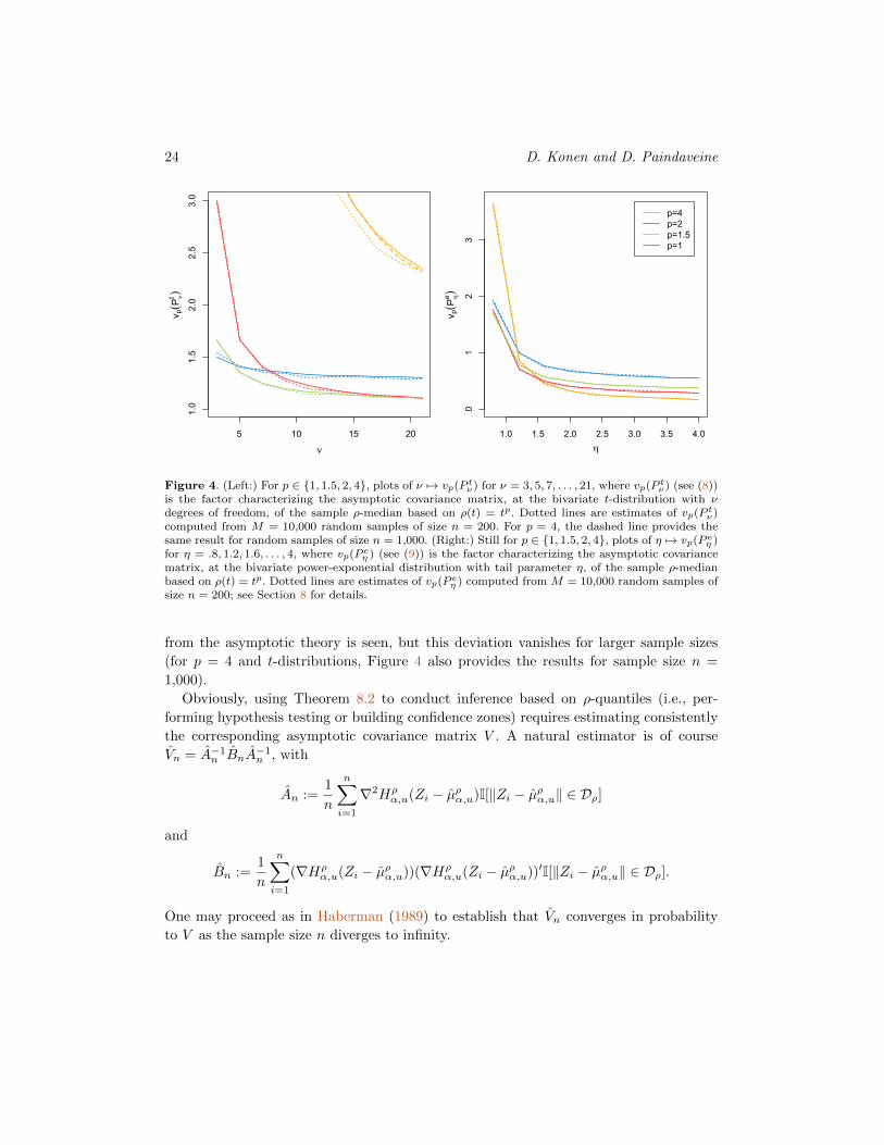
24 D. Konen and D. Paindaveine
5 10 15 20
1.0
1.5
2.0
2.5
3.0
ν
v p(P
νt )
1.0 1.5 2.0 2.5 3.0 3.5 4.0
01
23
ηv p(P
ηe )
p=4p=2p=1.5p=1
Figure 4. (Left:) For p ∈ {1, 1.5, 2, 4}, plots of ν 7→ vp(P tν) for ν = 3, 5, 7, . . . , 21, where vp(P tν) (see (8))is the factor characterizing the asymptotic covariance matrix, at the bivariate t-distribution with νdegrees of freedom, of the sample ρ-median based on ρ(t) = tp. Dotted lines are estimates of vp(P tν)computed from M = 10,000 random samples of size n = 200. For p = 4, the dashed line provides thesame result for random samples of size n = 1,000. (Right:) Still for p ∈ {1, 1.5, 2, 4}, plots of η 7→ vp(P eη )for η = .8, 1.2, 1.6, . . . , 4, where vp(P eη ) (see (9)) is the factor characterizing the asymptotic covariancematrix, at the bivariate power-exponential distribution with tail parameter η, of the sample ρ-medianbased on ρ(t) = tp. Dotted lines are estimates of vp(P eη ) computed from M = 10,000 random samples ofsize n = 200; see Section 8 for details.
from the asymptotic theory is seen, but this deviation vanishes for larger sample sizes
(for p = 4 and t-distributions, Figure 4 also provides the results for sample size n =
1,000).
Obviously, using Theorem 8.2 to conduct inference based on ρ-quantiles (i.e., per-
forming hypothesis testing or building confidence zones) requires estimating consistently
the corresponding asymptotic covariance matrix V . A natural estimator is of course
Vn = A−1n BnA−1n , with
An :=1
n
n∑i=1
∇2Hρα,u(Zi − µρα,u)I[‖Zi − µρα,u‖ ∈ Dρ]
and
Bn :=1
n
n∑i=1
(∇Hρα,u(Zi − µρα,u))(∇Hρ
α,u(Zi − µρα,u))′I[‖Zi − µρα,u‖ ∈ Dρ].
One may proceed as in Haberman (1989) to establish that Vn converges in probability
to V as the sample size n diverges to infinity.

Multivariate ρ-Quantiles 25
9. Perspectives for future research
In this paper, we investigated the properties of the spatial ρ-quantiles in Definition 1.
While this arguably settles the probabilistic study of these quantiles in the setup consid-
ered, our work naturally calls for an extension to more general setups and for applications
of these quantiles. As mentioned in the introduction, the spatial quantiles from Chaud-
huri (1996) are flexible objects that can cope with more exotic types of data, such as
functional data. This is associated with the fact that these quantiles are defined as min-
imizers of an objective function (see (1)) that involves norms and inner products only,
hence that also makes sense in Hilbert spaces. This, however, is also the case for the
objective function defining ρ-quantiles in (2), so that it would be natural to investigate
the properties of ρ-quantiles for random variables taking values in Hilbert spaces and to
compare their properties with those of the classical spatial quantiles; we refer to Cardot,
Cenac and Godichon-Baggioni (2017), Cardot, Cenac and Zitt (2013) and Chakraborty
and Chaudhuri (2014) for results on the spatial median and spatial quantiles in infinite-
dimensional spaces.
Another direction for future research is related to inferential applications. As al-
ready mentioned in the introduction, the spatial quantiles from Chaudhuri (1996) and
the companion spatial depth have been much used in a quantile regression framework
(Chakraborty (2003), Cheng and De Gooijer (2007), Chowdhury and Chaudhuri (2019)),
and it would be of interest to consider ρ-quantiles in this setup. In particular, this would
provide a spatial concept of multiple-output expectile regression, which would be quite
natural since expectiles were originally introduced, in Newey and Powell (1987), as an
L2-alternative to the traditional L1-concept of quantile regression (Koenker and Bassett
(1978)). Another natural venue for application of ρ-quantiles and ρ-depth is supervised
classification. In the last decade, supervised classification based on depth, where a new
observation is classified into the population with respect to which it is deepest, has met
much success in the literature; see, e.g., Li, Cuesta-Albertos and Liu (2012), Pokotylo,
Mozharovskyi and Dyckerhoff (2019), and the references therein. In this framework,
Lp-depths provide natural tools to implement this max-depth approach where p might
be chosen through cross-validation. Such applications, or the application of ρ-quantiles
in risk assessment, deserve a full-fledged paper, hence are left for future work.
Acknowledgement
The authors would like to thank the Editor-In-Chief, Mark Podolskij, the Associate
Editor, and two anonymous referees for their insightful comments and suggestions. This
research work was supported by a research fellowship from the Francqui Foundation
and by the Program of Concerted Research Actions (ARC) of the Universite libre de
Bruxelles.

26 D. Konen and D. Paindaveine
Supplementary Material
Technical proofs
(). This online supplement contains the proofs of all results stated in this paper.
References
Azzalini, A. and Capitanio, A. (2014). The Skew-Normal and Related Families. IMS
Monograph series. Cambridge University Press.
Boyd, S. and Vandenberghe, L. (2004). Convex Optimization. Cambridge University
Press, Cambridge.
Breckling, J. and Chambers, R. (1988). M-Quantiles. Biometrika 75 761–771.
Brown, B. M. (1983). Statistical uses of the spatial median. J. R. Statist. Soc. Ser. B
45 25–30.
Cardot, H., Cenac, P. and Zitt, P.-A. (2013). Efficient and fast estimation of the
geometric median in Hilbert spaces with an averaged stochastic gradient algorithm.
Bernoulli 19 18–43.
Cardot, H., Cenac, P. and Godichon-Baggioni, A. (2017). Online estimation of
the geometric median in Hilbert spaces: Nonasymptotic confidence balls. Ann. Statist.
45 591–614.
Chakraborty, B. (2003). On multivariate quantile regression. J. Statist. Plann. Infer-
ence 110 109–132.
Chakraborty, A. and Chaudhuri, P. (2014). The spatial distribution in infinite
dimensional spaces and related quantiles and depths. Ann. Statist. 42 1203–1231.
Chaudhuri, P. (1996). On a geometric notion of quantiles for multivariate data. J.
Amer. Statist. Assoc. 91 862–872.
Chen, Z. (1996). Conditional Lp-quantiles and their application to the testing of sym-
metry in non-parametric regression. Statist. Probab. Lett. 29 107–115.
Cheng, Y. and De Gooijer, J. G. (2007). On the uth geometric conditional quantile.
J. Statist. Plann. Inference 137 1914–1930.
Chowdhury, J. and Chaudhuri, P. (2019). Nonparametric depth and quantile regres-
sion for functional data. Bernoulli 25 395–423.
Daouia, A., Girard, S. and Stupfler, G. (2018). Estimation of tail risk based on
extreme expectiles. J. Roy. Statist. Soc. Ser. B 80 263–292.
Daouia, A., Girard, S. and Stupfler, G. (2019). Extreme M-quantiles as risk mea-
sures: from L1 to Lp optimization. Bernoulli 25 264–309.
Francisci, G., Nieto-Reyes, A. and Agostinelli, C. (2019). Generalization of the
simplicial depth: no vanishment outside the convex hull of the distribution support.
arXiv preprint arXiv:1909.02739.
Multivariate ρ-Quantiles 27
Gardes, L., Girard, S. and Stupfler, G. (2020). Beyond tail median and conditional
tail expectation: extreme risk estimation using tail Lp-optimization. Scand. J. Statist.
47 922–949.
Ghosh, A. K. and Chaudhuri, P. (2005). On maximum depth and related classifiers.
Scand. J. Stat. 32 327–350.
Girard, S. and Stupfler, G. (2015). Extreme geometric quantiles in a multivariate
regular variation framework. Extremes 18 629–663.
Girard, S. and Stupfler, G. (2017). Intriguing properties of extreme geometric quan-
tiles. REVSTAT 15 107–139.
Haberman, S. J. (1989). Concavity and estimation. Ann. Statist. 17 1631–1661.
Hallin, M., Paindaveine, D. and Siman, M. (2010). Multivariate quantiles and
multiple-output regression quantiles: From L1 optimization to halfspace depth (with
discussion). Ann. Statist. 38 635–703.
Hallin, M., del Barrio, E., Albertos, J. C. and Matran, C. (2021). Center-
outward distribution/quantile functions, ranks, and signs in Rd: a measure transporta-
tion approach. Ann. Statist. 49(2) 1139–1165.
Herrmann, K., Hofert, M. and Mailhot, M. (2018). Multivariate geometric expec-
tiles. Scand. Actuar. J. 2018 629–659.
Koenker, R. and Bassett, G. Jr. (1978). Regression quantiles. Econometrica 46
33–50.
Koltchinski, V. I. (1997). M-estimation, convexity and quantiles. Ann. Statist. 25
435–477.
Konen, D. and Paindaveine, D. (2021). Supplement to “Multivariate ρ-quantiles: a
spatial Approach”.
Kuan, C. M., Yeh, J. H. and Hsu, Y. C. (2009). Assessing value at risk with CARE,
the Conditional Autoregressive Expectile models. J. Econometrics 150 261–270.
Li, J., Cuesta-Albertos, J. A. and Liu, R. Y. (2012). DD-classifier: Nonparametric
classification procedure based on DD-plot. J. Amer. Statist. Assoc 107 737–753.
Magyar, A. and Tyler, D. E. (2011). The asymptotic efficiency of the spatial median
for elliptically symmetric distributions. Sankhya 73 165–192.
Masse, J.-C. (2002). Asymptotics for the Tukey median. J. Multivariate Anal. 81 286–
300.
Mosler, K. (2012). Multivariate Dispersion, Central Regions, and Depth: The Lift
Zonoid Approach 165. Springer Science & Business Media.
Mottonen, J., Nordhausen, K., Oja, H. et al. (2010). Asymptotic theory of the
spatial median. In Nonparametrics and Robustness in Modern Statistical Inference
and Time Series Analysis: A Festschrift in honor of Professor Jana Jureckova 182–
193. Institute of Mathematical Statistics.
Mukhopadhyaya, N. D. and Chatterjee, S. (2011). High dimensional data analysis
using multivariate generalized spatial quantiles. J. Multivariate Anal. 102 768–780.
28 D. Konen and D. Paindaveine
Newey, W. K. and Powell, J. L. (1987). Asymmetric least squares estimation and
testing. Econometrica 55 819–847.
Paindaveine, D. and Virta, J. (2021). On the behavior of extreme spatial quantiles
under minimal assumptions. In Advances in Contemporary Statistics and Econometrics
(A. Daouia and A. Ruiz-Gazen, eds.) 243–259. Springer, Cham.
Pokotylo, O., Mozharovskyi, P. and Dyckerhoff, R. (2019). Depth and depth-
based classification with R-package ddalpha. J. Statist. Softw. 91 1–46.
Serfling, R. (2002). Quantile functions for multivariate analysis: approaches and ap-
plications. Stat. Neerl. 56 214–232.
Serfling, R. (2010). Equivariance and invariance properties of multivariate quantile and
related functions, and the role of standardisation. J. Nonparametr. Stat. 22 915–936.
Serfling, R. (2019). Depth functions on general data spaces, I. Perspectives, with
consideration of “density” and “local” depths. Submitted.
Serfling, R. and Wijesuriya, U. (2017). Depth-based nonparametric description of
functional data, with emphasis on use of spatial depth. Comput. Statist. Data Anal.
105 24–45.
Serfling, R. and Zuo, Y. (2010). Discussion of “Multivariate quantiles and multiple-
output regression quantiles: From L1 optimization to halfspace depth”, by M. Hallin,
D. Paindaveine, and M. Siman. Ann. Statist. 38 676–684.
Taylor, J. (2008). Estimating value at risk and expected shortfall using expectiles. J.
Financ. Econometrics 6 231–252.
Usseglio-Carleve, A. (2018). Estimation of conditional extreme risk measures from
heavy-tailed elliptical random vectors. Electron. J. Stat. 12 4057–4093.
Vardi, Y. and Zhang, C.-H. (2000). The multivariate L1-median and associated data
depth. Proc. Natl. Acad. Sci. USA 97 1423–1426.
Zhou, W. and Serfling, R. (2008). Multivariate spatial U-quantiles: a Bahadur-Kiefer
representation, a Theil–Sen estimator for multiple regression, and a robust dispersion
estimator. J. Statist. Plann. Inference 138 1660–1678.