Embed Size (px)
Citation preview
MULTIVARIATE QUALITY CONTROL: STATISTICAL PERFORMANCE AND ECONOMIC FEASIBILITY
A Dissertation by
Mohammad Said Asem Khalidi
Masters of Science, Wichita State University, 1998
Bachelor of Science, Wichita State University, 1996
Submitted to the Department of Industrial and Manufacturing Engineering and the faculty of the Graduate School of
Wichita State University in partial fulfillment of
the requirements for the degree of Doctor of Philosophy
May 2007

© Copyright 2007 by Mohammad Said Asem Khalidi
All Rights Reserved
iii
MULTIVARIATE QUALITY CONTROL: STATISTICAL PERFORMANCE AND ECONOMIC FEASIBILITY
I have examined the final copy of this dissertation for form and content, and recommend that it be accepted in partial fulfillment of the requirement for the degree of Doctor of Philosophy with a major in Industrial Engineering ____________________________________ Gamal S. Weheba, Committee Chair We have read this dissertation and recommend its acceptance: ____________________________________ Abu S. Masud, Committee Member ____________________________________ M. Edwin Sawan, Committee Member ____________________________________ Michael Jorgensen, Committee Member ____________________________________ Haitao Liao, Committee Member
Accepted for the College of Engineering ____________________________________ Zulma Toro-Ramos, Dean Accepted for the Graduate School ____________________________________ Susan K. Kovar, Dean

iv
DEDICATION
To my beloved parents, Asem Khalidi and Hania Jauni,
for their continuous encouragement and unconditional support, which made the completion of this dissertation possible

v
ACKNOWLEDGMENTS
I am sincerely grateful to my advisor Dr. Weheba for his sustained guidance during the
course of my research and his heedful input towards this dissertation. He has been an inspiration
and an exceptional mentor during my graduate studies. His selfless role modeling has contributed
to my professional development.
Special thanks to the members of the advisory committee, Dr. Masud, Dr. Sawan, Dr.
Jorgensen, and Dr. Liao for their helpful comments and suggestions.
vi
ABSTRACT
Shewhart control charts have been used to monitor uncorrelated quality characteristics.
Advancement in manufacturing technology and increased complexity of products and systems
raise the need to monitor correlated characteristics. The literature provides numerous examples
of research pertaining to the misuse of traditional charts when the charted characteristics are
correlated. This research is aimed at quantifying the statistical and economic consequences of
utilizing the Hotelling’s T2 multivariate control chart as an alternative to the traditional
Shewhart⎯x chart. Consequently, there were two main objectives of this research. The first
objective was to identify the levels of correlation between the charted variables where the
statistical performance of the⎯x chart deteriorates compared to that of an equivalent T2 chart.
Statistical analyses of simulated data generated under varying levels of process and chart
variables indicated a correlation threshold value of + 0.48, outside of which the T2 chart is better.
The second objective was to assess the economic feasibility of utilizing a T2 chart as an
alternative to the two⎯x charts. Knappenberger and Grandage’s (1969), and Montgomery and
Klatt’s (1972) economic design models for⎯x and T2 charts were utilized, respectively, in
constructing an incremental cost model to examine the cost and worth of switching from the⎯x
charts to a T2 chart under specified levels of process and chart parameters. Results indicated that
the switch to multivariate T2 chart would result in economic savings under all levels of the
process and chart variables considered. It is hoped that this research will encourage practitioners
to implement appropriate multivariate statistical techniques in monitoring their processes.
vii
TABLE OF CONTENTS
Chapter Page 1 INTRODUCTION ....................................................................................................................1 2 LITERATURE REVIEW .........................................................................................................3
2.1 Traditional Statistical Process Control .............................................................................3 2.1.1 Capability in Univariate Domain..........................................................................5
2.2 Correlation........................................................................................................................7 2.3 Multivariate Statistical Process Control ........................................................................ 11
2.3.1 Hotelling T2 Control Charts............................................................................... 11 2.3.2 First Application................................................................................................ 15 2.3.3 Chart Interpretation ........................................................................................... 16 2.3.4 More Sensitive Charts ....................................................................................... 21 2.3.5 Capability in Multivariate Domain.................................................................... 24 2.3.6 Statistical Performance...................................................................................... 28 2.3.7 Advantages of Multivariate Statistical Process Control .................................... 31 2.3.8 Disadvantages of Multivariate Statistical Process Control ............................... 32
2.4 Economic Models.......................................................................................................... 32 2.4.1 Duncan’s Model ................................................................................................ 33 2.4.2 Lorenzen and Vance’s Model............................................................................ 34 2.4.3 Knappenberger and Grandage’s Model............................................................. 37
2.4.3.1 Montgomery and Klatt’s Approach to Multivariate T2 Chart............ 38
3 DISCUSSION........................................................................................................................ 40
3.1 Research Gap................................................................................................................. 43 3.2 Research Objectives ...................................................................................................... 44 3.3 Research Procedures...................................................................................................... 45
4 INITIAL INVESTIGATIONS............................................................................................... 48
4.1 Simulation Development and Verification.................................................................... 48 4.2 Data Analysis and Validation........................................................................................ 50
5 CHARACTERISTICS OF STATISTICAL PERFORMANCE ............................................ 58
5.1 Design Selection............................................................................................................ 59 5.2 Statistical Analysis ........................................................................................................ 64 5.3 Residual Analysis .......................................................................................................... 67 5.4 Interpretation ................................................................................................................. 72
viii
TABLE OF CONTENTS (continued) Chapter Page
6 ESTIMATION OF INCREMENTAL COST ........................................................................ 76
6.1 Model Performance ....................................................................................................... 80 6.2 Statistical Analysis ........................................................................................................ 86 6.3 Interpretation ................................................................................................................. 88
7 SUMMARY AND CONCLUSIONS .................................................................................... 93
7.1 Summary and Results .................................................................................................... 93 7.2 Future Research ............................................................................................................. 95
REFERENCES ............................................................................................................................ 96 APPENDICES .............................................................................................................................102
A. Probability of Type II Error (β) for Multivariate T2 Control Chart ..............................103 B. Illustrative Example of Economic Cost Model for Univariate⎯x Charts
Based on Knappenberger and Grandge's Model (1969) ...............................................105 C. Illustrative Example of Economic Cost Model for Multivariate T2 Charts Based on Montgomery and Klatt's Model (1972).........................................................115

ix
LIST OF TABLES
Table Page 4.1 Analysis of Variance (ANOVA): Type I Error Probability ............................................... 52 4.2 Analysis of Variance (ANOVA): Type II Error Probability.............................................. 55 5.1 Actual Values and Corresponding Coded Levels of the Process and Chart Variables ...... 62 5.2 Design Matrix..................................................................................................................... 62 5.3 ANOVA for Fitting the Model........................................................................................... 65 5.4 ANOVA for Lack of Fit ..................................................................................................... 65 5.5 Model Summary Statistics ................................................................................................. 66 5.6 ANOVA for Quadratic Model............................................................................................ 67 5.7 Confidence Interval - T2 ..................................................................................................... 75 5.8 Confidence Interval -⎯x ..................................................................................................... 75 6.1 Actual Values and Corresponding Coded Levels of the Process and Chart Variables ...... 81 6.2 Design Matrix..................................................................................................................... 83 6.3 ANOVA for the Model ...................................................................................................... 85 A.1 Probability of Type II Error (β) for Multivariate T2 Control Chart P = 4, α = 0.01 ...........103 A.2 Probability of Type II Error (β) for Multivariate T2 Control Chart P = 4, α = 0.05 ...........104
x
LIST OF FIGURES Figure Page 2.1 Ellipse control region ........................................................................................................ 20 2.2 Probability of Type I error (α) ........................................................................................... 29 2.3 Probability of Type II error (β) .......................................................................................... 30 2.4 Production cycle in Duncan’s model ................................................................................. 34 2.5 Production cycle in Lorenzen and Vance’s model............................................................. 36 3.1 Research procedure (Stage I) ............................................................................................. 45 3.2 Research procedure (Stage II) ............................................................................................ 46 4.1 Simulation procedure (Type I error) probability................................................................ 50 4.2 Simulation procedure (Type II error) probability .............................................................. 51 4.3 Simulated data: Type I error probability ............................................................................ 52 4.4 Chart type and correlation interaction plot......................................................................... 53 4.5 Simulated data: Type II error probability Shewhart⎯x chart.............................................. 54 4.6 Simulated data: Type II error probability multivariate T2 chart......................................... 55 4.7 Chart type and correlation interaction plot......................................................................... 56 5.1 Central composite design in three factors (X1, X2, X3) ....................................................... 60 5.2 Normal probability plot of residuals for Type II error ....................................................... 68 5.3 Residuals vs. predicted values............................................................................................ 69 5.4 Residuals vs. correlation level............................................................................................ 69 5.5 Residuals vs. shift magnitude............................................................................................. 70 5.6 Residuals vs. subgroup size ............................................................................................... 70 5.7 Residuals vs. alpha levels................................................................................................... 71
xi
LIST OF FIGURES (continued) Figure Page 5.8 Residuals vs. chart type...................................................................................................... 71 5.9 Subgroup size and shift interaction plot ............................................................................. 72 5.10 Alpha and shift interaction plot .......................................................................................... 73 5.11 Chart type and correlation interaction plot......................................................................... 74 6.1 Program listing: calculation of Type II error (β)................................................................ 78 6.2 Illustrative example by Anderson (1958) to verify Type II error (β) calculation .............. 79 6.3 Normal probability plot of residuals for (ΔE(C))............................................................... 86 6.4 Residuals vs. predicted values............................................................................................ 87 6.5 Cost coefficients, correlation, subgroup size and shift interaction plot ............................. 88 6.6 Cost coefficients, correlation, alpha and sampling frequency interaction plot .................. 90 6.7 Correlation coefficients, subgroup size, shift, and sampling frequency interaction plot ... 91 6.8 Cost coefficients, subgroup size, and sampling frequency interaction plot ....................... 92

xii
LIST OF SYMBOLS μ population mean vector
Σ population covariance matrix
X random vector of quality characteristics
T2 statistic plot on control chart
2)pn,p,(T −α upper α percentage point of Hotelling’s T2 distribution
S estimate of population covariance matrix
μ0 value of μ corresponding to the in-control state
μ1 value of μ corresponding to the in-control state
⎯X sample mean vector of quality characteristics
δ vector of difference between the in-control and out-of-control states
E(C1) expected cost per unit of sampling and testing
E(C2) expected cost per unit of investigating and correcting the process
E(C3) expected cost per unit associated with producing defectives
a1 fixed cost per sample
a2 per-unit cost of sampling
a3 mean cost of investigating and correcting a process which is out-of-control
a4 penalty cost of producing a defective units
k number of units produced between successive samples
λ-1 mean time between shifts to the out-of-control state
ρi conditional probability that the test procedure indicates that the process is out-of-control given that the process is in state μi (i = 0, 1)
xiii
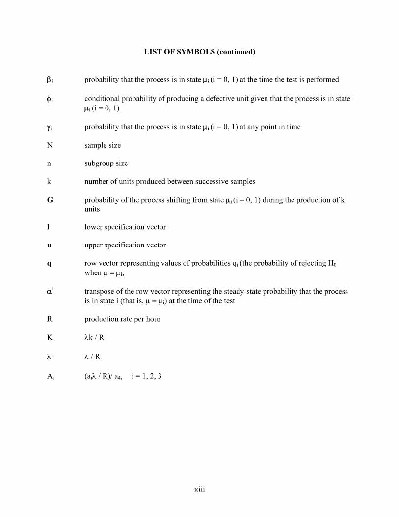
LIST OF SYMBOLS (continued) βi probability that the process is in state μi (i = 0, 1) at the time the test is performed
φi conditional probability of producing a defective unit given that the process is in state μi (i = 0, 1)
γi probability that the process is in state μi (i = 0, 1) at any point in time
N sample size
n subgroup size
k number of units produced between successive samples
G probability of the process shifting from state μi (i = 0, 1) during the production of k units
l lower specification vector
u upper specification vector
q row vector representing values of probabilities qi (the probability of rejecting H0 when μ = μi,
αt transpose of the row vector representing the steady-state probability that the process
is in state i (that is, μ = μi) at the time of the test R production rate per hour
K λk / R
λ` λ / R
Ai (aiλ / R)/ a4, i = 1, 2, 3
1
CHAPTER 1
INTRODUCTION
Since the pioneering work of Shewhart in 1931, control charts have been successfully
used to monitor process performance over time. They have been a foundation for maintaining
and achieving new unprecedented levels of quality. However, these are generally classified as
univariate charts that can only be used to monitor a single characteristic of a stationary process.
Advancements in technology and increased customer expectations have raised the need to
monitor correlated variables simultaneously. This requires the utilization of multivariate control
charts, enabling engineers and manufacturers to monitor the stability of their systems. Under
these conditions, achieving a state of statistical control requires a higher level of knowledge
regarding the process variables, the level of correlation among them, and the accuracy by which
they can be controlled. The original work in multivariate quality control can be attributed to
Hotelling (1947). His work led to a number of multivariate techniques presented in the
literature.
There are many situations where simultaneous monitoring or control of two or more
correlated quality characteristics is necessary. Using independent univariate charts is not always
the best method for monitoring correlated characteristics, because the correlations between
variables result in degrading the statistical performance of these charts.
With the advancement in technology and increased complexity of processes, customers’
demand of higher quality, and market competition, it is necessary to use multivariate statistical
process control (SPC). Furthermore, with the greatly increased availability of high-speed
computers and multivariate software, many users can now apply multivariate techniques.

2
Despite the renewed interest in multivariate SPC, these techniques have not been fully
utilized in practice. Some questions remain unanswered: the levels of correlation that mandate
the use of multivariate charts, and the statistical effect of mis-specifying the process model while
applying traditional Shewhart charts. In addition, the economic consequences of implementing
multivariate SPC as an alternative procedure to Shewhart charts have not been studied.
Chapter 2 presents a review of the literature of multivariate statistical process control and
the underlying assumptions. Chapter 3 provides a discussion leading to the research gap,
objectives, and procedures. Chapter 4 is devoted to the initial investigations to quantify the effect
of correlation on the statistical performance of the Shewhart⎯x chart and Hotelling T2 chart
leading to Chapter 5, which presents the characteristics of statistical performance of the
Shewhart⎯x chart and Hotelling T2 chart and their implementation boundaries. The incremental
cost model depicting the cost and worth of switching from Shewhart⎯x charts to Hotelling T2
chart is presented in Chapter 6. The summary and conclusions of this research including
recommended future research are provided in Chapter 7.

3
CHAPTER 2
LITERATURE REVIEW
This chapter presents a review of publications in the area of multivariate control charts
and their applications. This review is divided into four sections. The first section presents a
review of traditional statistical process control and process capability measures in the univariate
domain. The second section presents a definition of correlation and a review of the various
methods of quantifying its presence. The third section reviews multivariate statistical process
control methods, including a review of Hotelling T2 control charts and their schemes, the first
application of a Hotelling T2 control chart and its interpretation, a recent review of more
sensitive multivariate charts such as Multivariate Cumulative Sum (MCUSUM) and Multivariate
Exponentially Weighted Moving Average (MEWMA) control charts, a review of process
capability in the multivariate domain, and the statistical performance of Hotelling T2 control
charts. The fourth section presents a review of traditional economic models.
2.1 Traditional Statistical Process Control
Control charts were developed in 1931 by Shewhart to be utilized for process monitoring.
They have been widely used to distinguish between assignable causes and chance causes of
variation. The literature revealed several definitions of control charts. Shewhart (1931) gave the
control chart the following definition: “The control chart may serve, first, to define the goal or
standard for a process that management strives to attain; second, it may be used as an instrument
for attaining that goal and third, it may serve as a means of judging whether the goal has been
reached.” Control charts may also be viewed as a statistical tool as defined by Duncan in 1956:
“. . . a statistical device principally used for the study and control of repetitive processes.”
Moreover, Feigenbaum (1983) defined control charts as “. . . a graphical comparison of the
4
actual product-characteristics with limits reflecting the ability to produce as shown by past
experience on the product characteristics.”
Therefore, the control chart is a graphical display used to monitor a process. It usually
consists of a horizontal centerline corresponding to the in-control value of the parameter that is
being monitored and the lower and upper control limits. Control limits are not determined
arbitrarily, nor are they related to specification limits but rather by statistical criteria. If the
sample points fall within the control limits, the process is deemed to be in-control, or free from
any assignable causes. Points beyond the control limits indicate an out-of-control process, i.e.,
assignable causes are likely present. This signals the need for a corrective action to find and
remove the assignable causes. The assignable causes, also called special causes, are the portion
of the variability in a set of observations that can be traced to specific causes, such as, operators,
materials, or equipment. On the other hand, the chance causes, also called common causes, are
the portion of the variability in a set of observations that is due only to random forces and cannot
be traced to specific sources, such as, operators, materials, or equipment.
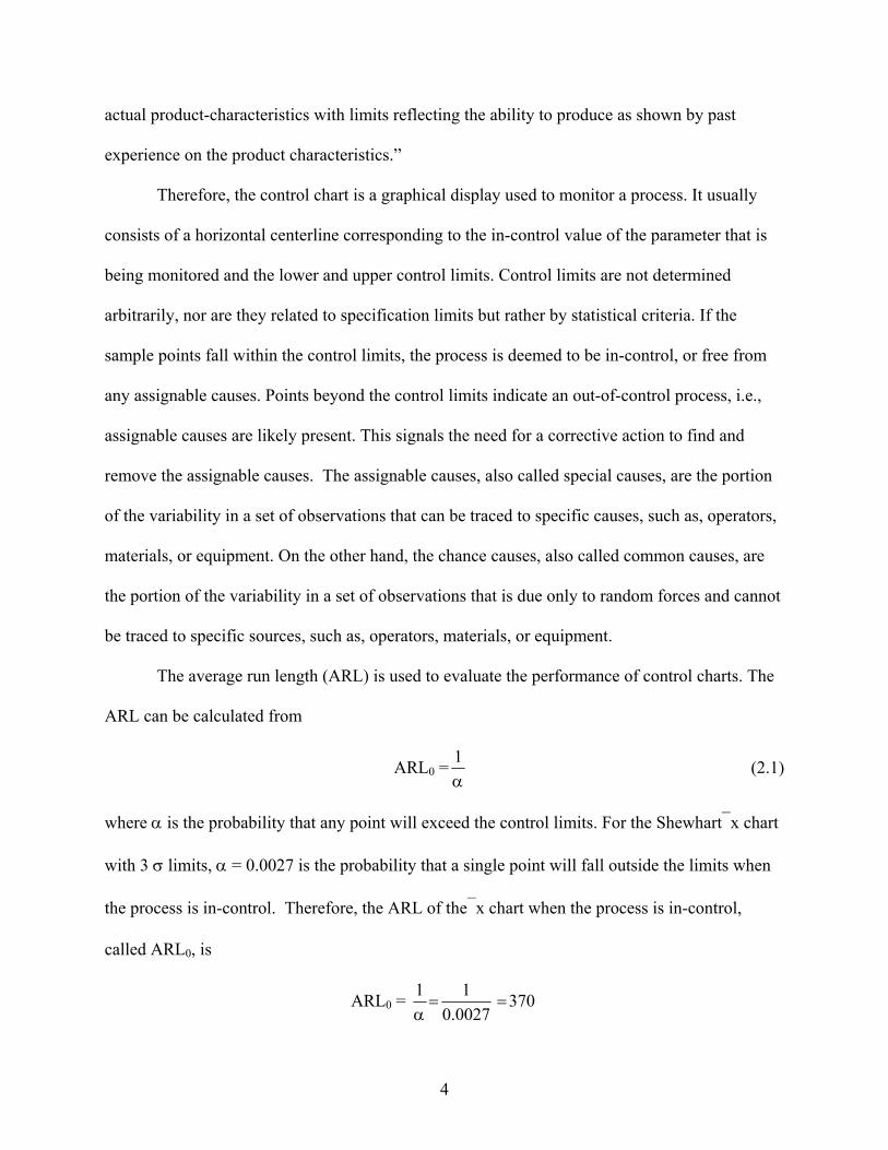
The average run length (ARL) is used to evaluate the performance of control charts. The
ARL can be calculated from
ARL0 =α1 (2.1)
where α is the probability that any point will exceed the control limits. For the Shewhart⎯x chart
with 3 σ limits, α = 0.0027 is the probability that a single point will fall outside the limits when
the process is in-control. Therefore, the ARL of the⎯x chart when the process is in-control,
called ARL0, is
ARL0 = 3700027.011
==α
5
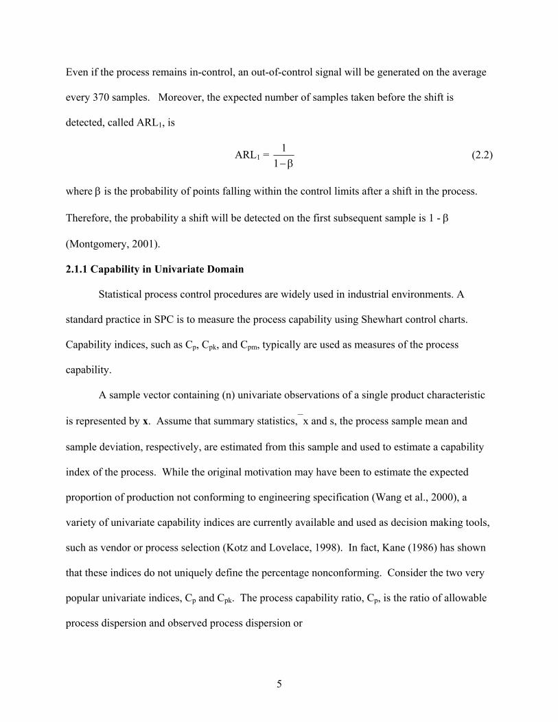
Even if the process remains in-control, an out-of-control signal will be generated on the average
every 370 samples. Moreover, the expected number of samples taken before the shift is
detected, called ARL1, is
ARL1 = β−1
1 (2.2)
where β is the probability of points falling within the control limits after a shift in the process.
Therefore, the probability a shift will be detected on the first subsequent sample is 1 - β
(Montgomery, 2001).
2.1.1 Capability in Univariate Domain
Statistical process control procedures are widely used in industrial environments. A
standard practice in SPC is to measure the process capability using Shewhart control charts.
Capability indices, such as Cp, Cpk, and Cpm, typically are used as measures of the process
capability.
A sample vector containing (n) univariate observations of a single product characteristic
is represented by x. Assume that summary statistics,⎯x and s, the process sample mean and
sample deviation, respectively, are estimated from this sample and used to estimate a capability
index of the process. While the original motivation may have been to estimate the expected
proportion of production not conforming to engineering specification (Wang et al., 2000), a
variety of univariate capability indices are currently available and used as decision making tools,
such as vendor or process selection (Kotz and Lovelace, 1998). In fact, Kane (1986) has shown
that these indices do not uniquely define the percentage nonconforming. Consider the two very
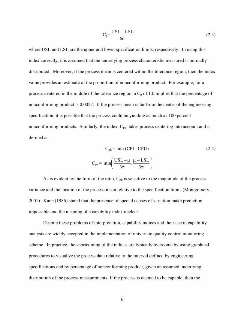
popular univariate indices, Cp and Cpk. The process capability ratio, Cp, is the ratio of allowable
process dispersion and observed process dispersion or
6
Cp=σ−
6LSLUSL (2.3)
where USL and LSL are the upper and lower specification limits, respectively. In using this
index correctly, it is assumed that the underlying process characteristic measured is normally
distributed. Moreover, if the process mean is centered within the tolerance region, then the index
value provides an estimate of the proportion of nonconforming product. For example, for a
process centered in the middle of the tolerance region, a Cp of 1.0 implies that the percentage of
nonconforming product is 0.0027. If the process mean is far from the center of the engineering
specification, it is possible that the process could be yielding as much as 100 percent
nonconforming products. Similarly, the index, Cpk, takes process centering into account and is
defined as
Cpk = min (CPL, CPU) (2.4)
Cpk = ⎟⎠⎞
⎜⎝⎛
σ−μ
σμ−
3LSL,
3USLmin
As is evident by the form of the ratio, Cpk is sensitive to the magnitude of the process
variance and the location of the process mean relative to the specification limits (Montgomery,
2001). Kane (1986) stated that the presence of special causes of variation make prediction
impossible and the meaning of a capability index unclear.
Despite these problems of interpretation, capability indices and their use in capability
analysis are widely accepted in the implementation of univariate quality control monitoring
scheme. In practice, the shortcoming of the indices are typically overcome by using graphical
procedures to visualize the process data relative to the interval defined by engineering
specifications and by percentage of nonconforming product, given an assumed underlying
distribution of the process measurements. If the process is deemed to be capable, then the
7
computed index value and the estimated percentage of nonconforming product are acceptable.
The acceptance regions for both these statistics are usually specified as part of an organization’s
quality control system.
By examining the graphical displays of the estimated distribution functions in
comparison to engineering specifications, the ambiguity of the univariate capability indices can
be explained. Therefore, it is reasonable to compare the bell-shaped curve of the assumed
normal distribution to the location of the upper and lower specification limits. The univariate
indices provide a comparison of the length of the intervals (Walpole and Myers, 1993).
However, in the multivariate domain, the comparison is somewhat more complex.
2.2 Correlation
The use of statistical process control has spread widely in industrial applications for
improving processes, estimating process parameters, and determining capability. A primary
assumption in the typical application of the standard Shewhart control charts is that observations
are independent or uncorrelated. Moreover, processes may be classified as stationary or non-
stationary. For stationary processes, Shewhart univariate charts are used to monitor single
variables. On the other hand, non-stationary processes are autocorrelated (Del Castillo, 2002).
Thus, an autocorrelated variable is a variable that is correlated “with itself” over time.
Unfortunately, the independent assumptions are often violated in many types of manufacturing
and production processes.
Correlation analysis is a statistical technique that can show whether and how strongly
pairs of variables are related. Correlation refers to the departure of two or more variables from
independence (Del Castillo, 2002). It is the degree to which two or more quantities are
associated (Montgomery, 2001). For example, height and weight are related; taller people tend
8
to be heavier than shorter people. However, people of the same height vary in weight; moreover,
there are people where the shorter one is heavier than the taller one. Nevertheless, the average
weight of people 5'5'' tall is less than the average weight of people 5'6'' tall, and their average
weight is less than that of people 5'7'' tall, and so on. Correlation can tell just how much of the
variation in peoples' weights is related to their heights and whether this relationship is adversely
or positively proportional. Correlation in industrial process data could be elucidated the same
way.
Although correlation is fairly obvious in some industrial processes data, many may
contain unsuspected correlations. Also correlations may be suspected without knowing which are
the strongest. A correlation analysis can lead to a greater understanding of such data. Like all
statistical techniques, correlation analysis is only appropriate for certain types of data, in which
numbers are meaningful, usually quantities of some sort. It cannot be used for purely categorical
data, such as gender. Various methods are used to quantify the presence of correlation.
When two or more random variables are defined on a probability space, it is usful to
describe how they vary together; that is, it is useful to measure the relationship between the
variables. A common measure of the relationship between two random variables is the
covariance. The covariance between random variables X and Y, denoted as cov (X, Y) or σxy is
σxy = E[(X - μX) (Y - μY)] (2.5)
Covariance gives an idea of the strength of the correlation. For two variables X and Y, if
the correlation is very strong means that if X is far from its mean, so should Y. Therefore, the
covariance between X and Y describes the variation between the two variables. In the
multivariate domain, the population covariance is represented in a matrix denoted as Σ. The
covariance matrix, also called the variance-covariance matrix, is a symmetrical matrix that
9
contains the variance and covariance among a set of random variables. The main diagonal
elements of the matrix are the variances of the random variables, and the off-diagonal elements
are the covariance between the p variables (Neter et al., 1996). The (p x p) sample variance-
covariance matrix S is formed as
S =
⎥⎥⎥⎥⎥
⎦
⎤
⎢⎢⎢⎢⎢
⎣
⎡
21
22212
1122
1
PP
P
P
SS
SSSSSS
LL
MLMM
L
L
(2.6)
In a two-dimensional plot, the degree of correlation between the values on the two axes is
quantified by the so-called correlation coefficient. The most common correlation coefficient is
the Pearson Product-Moment Correlation Coefficient, which is found by dividing the covariance
of the two variables by the product of their standard deviation. This correlation coefficient (r) is
a measure of the degree of linear relationship between two variables X and Y. In regression, the
emphasis is on predicting one variable from the other; in correlation, the emphasis is on the
degree to which a linear model may describe the relationship between two variables. In
regression, the interest is directional, one variable is predicted and the other is the predictor. On
the other hand, in correlation, the interest is non-directional; the relationship is the critical aspect.
The square of (r) is called the Coefficient of Determination and denotes the portion of total
variance explained by the regression model (Walpole and Myers, 1993). The sample correlation
coefficient (r) is calculated by
( )( )( ) yx
iixy ss1n
yyxxr
−−−
= ∑ (2.7)
10
where x and y are the sample means of xi and yi , sx and sy are the sample standard deviation of
xi and yi, and the sum is from i = 1 to (n). As for the population, the correlation coefficient ρxy
can be estimated from the sample xyr and defined as
( )YX
XY
YXxy
YXCOVσσ
σσσ
ρ ==, (2.8)
The correlation coefficient may take any value between - 1.0 and + 1.0. It is because of
Cauchy-Schwarz inequality that the correlation cannot exceed 1 in absolute value (Neter et al.,
1996). It is a useful inequality encountered in many different settings, such as linear algebra
applied to vectors, in analysis applied to infinite series, integration of products, and in probability
theory applied to variance and covariance. The inequality states that if x and y are elements of
real or complex inner product space, then
2)y,x( ≤ (x,x) (y,y) (2.9)
The two sides are equal if and only if x and y are linearly dependent (or parallel). This
contrasts with a property that the inner product of two vectors is zero if they are orthogonal (or
perpendicular) to each other (Johnson and Wichern, 1998).
A correlation coefficient of (r = 0.50) indicates a stronger degree of linear relationship
than one of (r = 0.40). Likewise, a correlation coefficient of (r = -0.50) shows a greater degree of
relationship than one of (r = -0.40). Thus, a correlation coefficient of zero (r = 0.0) indicates the
absence of a linear relationship and correlation coefficients of (r = +1.0) and (r = -1.0) indicate a
perfect linear relationship.
A limitation to the measures of correlation presented is noted; their value could be 0
while, in fact, there is a relationship between the variables. The reason may be because this
11
relationship is quadratic or of a higher order. Thus, it should be noted that correlation measures
represent the strength of the linear relationship of the variables (Neteret al., 1996).
2.3 Multivariate Statistical Process Control
Process monitoring using control charts can be seen as a two-stage process, Phase I and
Phase II (Woodall, 2000). The goal of Phase I is to evaluate the stability of the process and, after
coping with any assignable causes, to estimate the in-control values of the process parameters.
In Phase II, the main concern is to monitor the online data to quickly detect shifts in the process
from the baseline established in Phase I. Different types of statistical methods are appropriate
for the two phases, with each type requiring different measures of statistical performance. In
Phase I, it is important to assess the probability of deciding that the process is unstable.
However, in Phase II, the emphasis is on detecting process changes as quickly as possible. This
is usually measured by parameters of the run-length distribution, where the run length is the
number of samples taken before an out-of-control signal is given. The average run length is
often used to compare the performance of computing control chart methods.
Hotelling (1947) developed the multivariate T2 control chart as a direct analog of the
Shewhart⎯x control chart. This chart can be used to monitor the mean vector of multiple quality
characteristics of a process in both Phase I and Phase II operations.
2.3.1 Hotelling T2 Control Charts
The multivariate process control problem involves a repetitive process in which each
characteristic is represented by random variables, X1, X2, …, Xp. The probability distribution of
the process characteristics is assumed to be multivariate normal with a mean vector μ and a
covariance matrix Σ. Multiple measurements of each process are assumed to be drawn from a
population with standard values for μ0 and Σ0. When changes in the process cause elements of μ
12
or Σ to shift from the standard values, it is necessary to detect and correct the change to ensure a
stable process.
The T2 control chart combines several quality characteristics for each item into a single
quality measurement of the overall performance of the item. Hotelling formulated T2 on the basis
of a generalized Student Ratio (t) that was introduced in 1931 for testing multivariate hypotheses
when the sample variance-covariance matrix S is unknown. Hotelling applied T2 to the quality-
control problem of testing bombsights. The advantage of the T2 control chart is that the status of
the process can be characterized by one value. However, if an out-of-control process does exist,
one must go back to the original data to determine the nature of this problem.
In controlling industrial processes, it is not sufficient to monitor only the process mean.
The process variability should be monitored and controlled as well. Montgomery and
Wadsworth (1972) proposed a control chart for the multivariate dispersion that is based on a
normal approximation of log |S|, where S is the sample variance-covariance matrix. This chart
can be constructed by using data from the same preliminary samples used to develop the T2
control chart. The variance-covariance matrix for each sample can then be computed from
preliminary samples. To construct the log |S| chart, first the determinant of the variance-
covariance matrix for each sample is computed, then the logarithm of the determinant of each of
these matrices is taken, and the mean and standard deviation of this logarithm is determined. A
control chart can then be constructed using the upper control limit (UCL) and the lower control
limit (LCL) calculated as
UCL = Y + 2
αZ Sy (2.10)
LCL = Y - 2
αZ Sy (2.11)
13
where 2
αZ is the percentage point of the normal distribution, and⎯Y and Sy are the mean and the
standard deviation of the logarithm of the determinant of each variance-covariance matrix. This
chart, in conjunction with the T2 control chart, could monitor, diagnose, and control procedures
for multivariate control between and within sample variations.
Assume that there are (p) process characteristics that are jointly distributed according to
the p-variate normal distribution, and a random sample of size (n) is available from the process.
Then the multivariate analogue of (t) is
( )
ns
Xt 2
202 μ−
= (2.12)
t2 = n ( ) ( ) ( )00 μXsμX −′−−12
When t2 is generalized to (p) variables, it becomes
T2 = n ( ) ( )( )01
0 μXΣμX 0 −′− − (2.13)
where
μ0 is a (p x 1) vector of population mean
⎯X is a (p x 1) vector of sample mean
Σ0 is a (p x p) variance-covariance matrix
If the observed statistical distance T2 is too large, that is, if⎯X is “too far” from μ0, then the
hypotheses H0: μ = μ0 is rejected. Since T2 is distributed as pn
np−
− )1(),( pnpF −α , then the T2
statistic can be used for testing the hypotheses about the mean vector μ0 such as
H0 : μ = μ0
14
H1 : μ ≠ μ0
T2 can be computed and compared with pn
np−
− )1( ),( pnpF −α
When multiplying a T2 statistic by a constant ( )( )( )1n1np
pnn−+
− , it follows an F-distribution, where
),( pnpF −α refers to the F-distribution with (p) and (n – p) degrees of freedom and a probability of
Type 1 error ofα . The null hypothesis would be rejected if
T2 > pn
np−
− )1(),( pnpF −α (2.14)
Thus, the control limits of the T2 control chart can be formed as
UCL = pn
np−
− )1(),( pnpF −α (2.15)
and
LCL = 0 (2.16)
Since the test statistic is a generalized measurement of distance, the lower control limit is
always zero. The reason for this is that any shift in the mean will always lead to an increase in
the T2 statistic, and thus the LCL may be ignored. If the computed statistic T2 exceeds the upper
control limit, the process mean is out-of-control, and assignable causes of variation are sought. In
practice, μ0 is generally unknown, so it is necessary to estimate it from a set of preliminary
samples, which are taken when the process is assumed to be in-control.
If μ0 and Σ0 are estimated from a relatively large number (more than 25) of preliminary
samples, then it is customary to use 2, pαχ as the upper control limit on the T2 control chart, where
15
2, pαχ is the upper α percentage point of the Chi-square distribution with (p) degrees of freedom
(Montgomery, 2001).
2.3.2 First Application
Hotelling (1947) conducted a study on dropping bombs from airplanes for the purpose of
testing bombsights. Air testing is only one in a series of tests and inspections to which a
bombsight is subjected. It is the final step and an exceptionally costly one. Because of the high
cost and uncertainty of air testing with relative accuracy, only a very small number of
bombsights were tested. Two sights were randomly selected from each lot of twenty sights. Four
bombs on each sight from two flights were dropped for this experiment. Two measurements
were targeted for the accuracy of each bomb dropping. The range error is an error in the direction
of the airplane’s heading at the time of releasing the bombs on the sights. The deflection error is
an error in a direction perpendicular to the airplane’s heading to the bombsight location.
There were three testing alternatives. The first alternative was to accept the bomb sight for
which the univariate scheme applied for acceptance. Hence, the probability of Type I error (α) is
maintained on each scheme. The true probability of Type I error for the joint control procedure is
α’ = 1 - (1 - α)p. Therefore, the probability that both range and deflection are acceptable for α =
0.0027 is
(2.17)
Another alternative was rejection, which would require that both variables take such
values as to call for rejection. For two independent variables, a probability of rejection intended
to be 0.9 would actually be only 0.81in such a case. Thus, rejection occurs if both range and
deflection are unacceptable. For β = 0.10,
(2.18)
( ) 9946.09973.0)0027.01()Acceptance(P 22 ==−=
81.0)10.01()Rejection(P 2 =−=
16
Hotelling suggested that the probabilities could be adjusted so as to become equal to 0.05,
or such level as is chosen, by altering the acceptance level for each variable separately.
However, this introduces additional difficulties. The variables may not be mutually independent,
and calculations such as the aforementioned must be altered to take into account the multivariate
distribution. Furthermore, it will often not be known whether they are independent or not; or if
they are mutually dependent, the character of the dependence may be known only imperfectly.
Thus, the correlation coefficient may have to be estimated from the preliminary sample size, so
small as to leave its value somewhat uncertain. Any acceptance probabilities based on such a
correlation coefficient will then, likewise, be uncertain. Another defect of such assumptions
mentioned earlier is that an article close to the margin of acceptability with respect to one
variable may well be marked for acceptance or rejection on the basis of the other variable
involved. Unusual excellence in one respect may often occur for a slight departure in another
way from what would otherwise be considered satisfactory.
As a result, Hotelling proposed a third alternative, which was a combined measure of
accuracy T2 that serves as a measure of the deviation of the particular bomb from the center of
the target. This measure is more accurately interpreted in terms of the probability than is the
actual distance. By adding the values of T2 for all bombs dropped on a particular bombsight, a
measure is useful in obtaining the accuracy of the bombsight, which achieves specified levels of
(α) and (β) risks (Hotelling, 1947).
2.3.3 Chart Interpretation
The objective of performing multivariate SPC is to monitor process performance over
time in order to detect any unusual events. It is essential to be able to track the cause of an out-
of-control signal to maintain acceptable levels of quality and to allow for process improvements.
17
However, the complexity of multivariate control charts and cross-correlation among variables
makes it difficult to analyze assignable causes leading to the out-of-control signals. Several
techniques have been developed that assist in the interpretation of out-of-control signals.
Following the same sensitivity of the Shewhart⎯x control chart, the Hotelling T2 is more efficient
in detecting larger process shifts. Mason and Young (1999) introduced a modification procedure
for the T2 control charts in order to enhance sensitivity toward detecting a small process shift.
A T2 control chart is used primarily to monitor the mean vector of quality characteristics
of a process. There are two versions of the T2 chart, one for subgrouped data and the other for
individual observations. They can be used not only in achieving a state of statistical control
(Phase I) but also in maintaining control over the process (Phase II).
In some cases, the multivariate data can be grouped into rational subgroups, relying on
properties of the production process that creates homogeneity within subgroups. When rational
subgroups are present, a shift in the mean vector is presumed to be more likely to take place
between subgroups (variability in the process over time) than within a subgroup (instantaneous
process variability at a given time). This can be used to advantage by forming the sample
covariance matrix for each subgroup, then averaging them to get an estimate of the process
covariance matrix. The mean vectors for each subgroup can be examined for a shift, thus
detecting assignable causes for the shift in the mean vector (Sullivan and Woodall, 1996).
Mason et al. (2001) studied the effectiveness of using the T2 control charts for batch
(subgrouped) processes. His study recommended that when the batch data are collected from the
same multivariate normal distribution, T2 statistic is recommended for detecting out-of-control
signals. When the batch data are collected from multivariate normal distributions with different
mean vectors, the translation of the different batches to a common origin again allows the usage

18
of T2 statistic to identify out-of-control signals. Translation to a common origin involves the
subtraction of individual batch mean vectors from the corresponding batch observations.
However, sometimes the rational subgroup size is one, that is, data are structured only as
individual observations, and process characteristics do not necessarily produce homogeneous
subgroups of large size. In the case of individual observations, Sullivan and Woodall (1996)
recommended using the sample mean vector and covariance matrix if any value of the T2 statistic
exceeds an upper control limit resulting in an out-of-control signal generated. In some industrial
situations, such as chemical and process industries, it is either impractical or difficult to obtain a
subgroup size of more than one unit, since these industries frequently have multiple quality
characteristics that must be monitored. Therefore, the T2 control chart with n = 1 would be
appropriate to use.
Mason et al. (1997) presented a multivariate profile chart by superimposing an⎯x chart of
univariate statistics on top of the T2 chart. By performing discrimination analysis, this allows the
distinguishing of in-control conditions from out-of-control conditions to determine where
assignable causes of variation are occurring. This analysis works by partitioning the multivariate
control chart based on the contribution of each variable.
There are also graphical solutions to interpretation difficulty. Lowry and Montgomery
(1995) proposed poly plots and multivariate control webs to superimpose univariate statistics on
multivariate statistics in order for the user to test trends in individual statistics and realize how
they affect other variables.
Jackson (1956) suggested that the multivariate control region be displayed as an ellipse
for two variables (p = 2). However, when Jackson’s control ellipse is used, the time sequence of
the plotted points is lost. The results obtained from Jackson’s control ellipse are exactly the
19
same as those obtained from using the T2 control chart. If an observation is outside the ellipse, it
will also be above the control limit specified on the T2 control chart. On the other hand, if an
observation is inside the control ellipse, it will be below the control limit specified on the T2
control chart. However, if an observation is exactly on the parameter of the ellipse, it will be
exactly on the control limit line of the T2 control chart. The results obtained by both methods
are identical. Nevertheless, the T2 control chart retains the time scale and summarizes the
process condition by one value, while use of the control ellipse indicates pictorially the nature of
the out-of-control conditions.
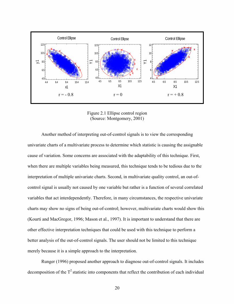
Figure 2.1 presents the control region for two variables with different levels of
correlations. Here, it can be seen that when (r = + 0.8), the control ellipse is tilted to the right
from the horizontal axis; on the other hand, when (r = - 0.8), the ellipse becomes tilted to the left
from the horizontal axis. However, when (r = 0), the ellipse becomes a circle.
Jackson (1959) considered the case of investigating two or more (p - 1) related variables
to analyze a multivariate process. The basic concept of the technique is to break up the T2
statistic into a sum of its principal components, the linear portions of the original variables.
Principal component analysis (PCA) is a reliable technique to interpret out-of-control signals,
whereby components can be examined to understand why the process is out-of-control. This
could be accomplished by expressing the T2 statistic as the normalized principal component of
the multinormal variables. Hence, when an out-of-control signal is received, components with
abnormally high values are detected. Plots of these variables can be used to determine exactly
what occurred in the original sets of data that contributed to the signal in the multivariate set of
T2 statistics (Mason et al., 1997).
20
Control Ellipse
4.4 6.4 8.4 10.4 12.4
x1
4.5
6.5
8.5
10.5
12.5
y1Control Ellipse
4.5 6.5 8.5 10.5 12.5
X1
4.5
6.5
8.5
10.5
12.5
Y1
Control Ellipse
4.5 6.5 8.5 10.5 12.5
X1
4
6
8
10
12
Y1
r = - 0.8 r = 0 r = + 0.8
Figure 2.1 Ellipse control region (Source: Montgomery, 2001)
Another method of interpreting out-of-control signals is to view the corresponding
univariate charts of a multivariate process to determine which statistic is causing the assignable
cause of variation. Some concerns are associated with the adaptability of this technique. First,
when there are multiple variables being measured, this technique tends to be tedious due to the
interpretation of multiple univariate charts. Second, in multivariate quality control, an out-of-
control signal is usually not caused by one variable but rather is a function of several correlated
variables that act interdependently. Therefore, in many circumstances, the respective univariate
charts may show no signs of being out-of-control; however, multivariate charts would show this
(Kourti and MacGregor, 1996; Mason et al., 1997). It is important to understand that there are
other effective interpretation techniques that could be used with this technique to perform a
better analysis of the out-of-control signals. The user should not be limited to this technique
merely because it is a simple approach to the interpretation.
Runger (1996) proposed another approach to diagnose out-of-control signals. It includes
decomposition of the T2 statistic into components that reflect the contribution of each individual

21
variable. The variable with the relatively higher contribution to the overall statistic should be the
focus of attention.
2.3.4 More Sensitive Charts
Hotelling’s multivariate control chart procedure is based on only the most recent
observation; it is insensitive to small and moderate shifts in the mean vector. Hotelling’s work
paved the way for further developments in the multivariate field. Several multivariate CUSUM
and multivariate EWMA procedures have appeared in the literature since then.
2.3.4.1 Multivariate CUSUM Control Charts
The Cumulative Sum (CUSUM) chart was first developed by Page (1954) to detect slight
but sustained shifts in the process level (1.5 σ or less). The CUSUM chart is constructed for
monitoring the mean of a process. It can be constructed for both individual observations n = 1
and the averages of rational subgroups n > 1 (Johnson, 1994). The multivariate CUSUM
(MCUSUM) chart can be derived from the univariate versions to serve multivariate process
monitoring purposes. There are two different approaches of applying CUSUM: one is the
simultaneous analysis of multiple univariate CUSUM procedures; the other involves modifying
the CUSUM scheme itself to form MCUSUM procedures. A MCUSUM can be derived from
CUSUM based on two strategies. The first strategy involves reducing each multivariate
observation to a weighted measurement and then forming a CUSUM of these measurements. The
second strategy involves forming a MCUSUM directly from the observations by accumulating
the X vectors before reducing it to weighted measurements. MCUSUM procedures are mostly
dependent on the non-centrality parameter, which reports the shift size in terms of a quantity and
defined as
τ = (μ’ Σ−1 μ)1/2 (2.19)
22
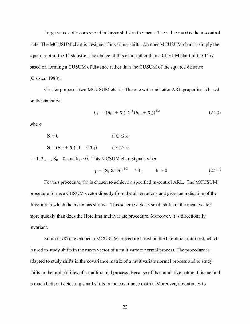
Large values of τ correspond to larger shifts in the mean. The value τ = 0 is the in-control
state. The MCUSUM chart is designed for various shifts. Another MCUSUM chart is simply the
square root of the T2 statistic. The choice of this chart rather than a CUSUM chart of the T2 is
based on forming a CUSUM of distance rather than the CUSUM of the squared distance
(Crosier, 1988).
Crosier proposed two MCUSUM charts. The one with the better ARL properties is based
on the statistics
Ci = {(Si-1 + Xi)` Σ-1 (Si-1 + Xi)}1/2 (2.20)
where
Si = 0 if Ci ≤ k1
Si = (Si-1 + Xi) (1 – k1/Ci) if Ci > k1
i = 1, 2,…., S0 = 0, and k1 > 0. This MCSUM chart signals when
γi = {Si` Σ-1 Si}1/2 > h, h > 0 (2.21)
For this procedure, (h) is chosen to achieve a specified in-control ARL. The MCUSUM
procedure forms a CUSUM vector directly from the observations and gives an indication of the
direction in which the mean has shifted. This scheme detects small shifts in the mean vector
more quickly than does the Hotelling multivariate procedure. Moreover, it is directionally
invariant.
Smith (1987) developed a MCUSUM procedure based on the likelihood ratio test, which
is used to study shifts in the mean vector of a multivariate normal process. The procedure is
adapted to study shifts in the covariance matrix of a multivariate normal process and to study
shifts in the probabilities of a multinomial process. Because of its cumulative nature, this method
is much better at detecting small shifts in the covariance matrix. Moreover, it continues to

23
operate well for large shifts in variability. When a trend occurs in one direction of the target
mean and a resulting shift occurs in the other direction, the MCUSUM chart will not detect the
shift immediately. A combination of the MCUSUM chart and the T2 limits will improve the chart
sensitivity to large shifts (Lowry and Montgomery, 1995).
2.3.4.2 Multivariate EWMA Control Charts
The scheme of the exponentially weighted moving average chart developed by Roberts
(1959), is similar to the moving average chart and could be extended to multivariate quality
control problems (Montgomery, 2001). Shewhart’s control charts have been the traditional tools
for detecting larger shifts in the process mean (1.5 σ or more). For the univariate case, the
EWMA is more effective than Shewhart control charts in detecting smaller shifts in the process
mean. When (n) measurements from each item are required, these univariate control charts
ignore the dependency among the (p) variables.
The multivariate exponentially weighted moving average control chart accumulates
information from past observations making it sensitive to shifts in the variance as well as shifts
in the mean. It allows the user to specify weights for each variable being measured. Although
MEWMA is used commonly for controlling a multivariate process mean, Alt and Smith (1988)
proposed three control charts for monitoring the covariance matrix, which is analogous to
EWMA for the variance. Prabu and Runger (1997) have provided a thorough analysis of the
average run-length performance of the MEWMA control chart. The MEWMA chart given by
Lowry et al. (1992) is a natural extension to the univariate EWMA, defined by vectors of
EWMAs and based on the statistics as
Gi = λ xi + (1 - λ) Gi-1 (2.22)
where G0 = 0, 0 < λj ≤ 1.0, and i = 1, 2, …, λ = diagonal (λ1, λ2, …, λp), and j = 1, 2, …, p.
24
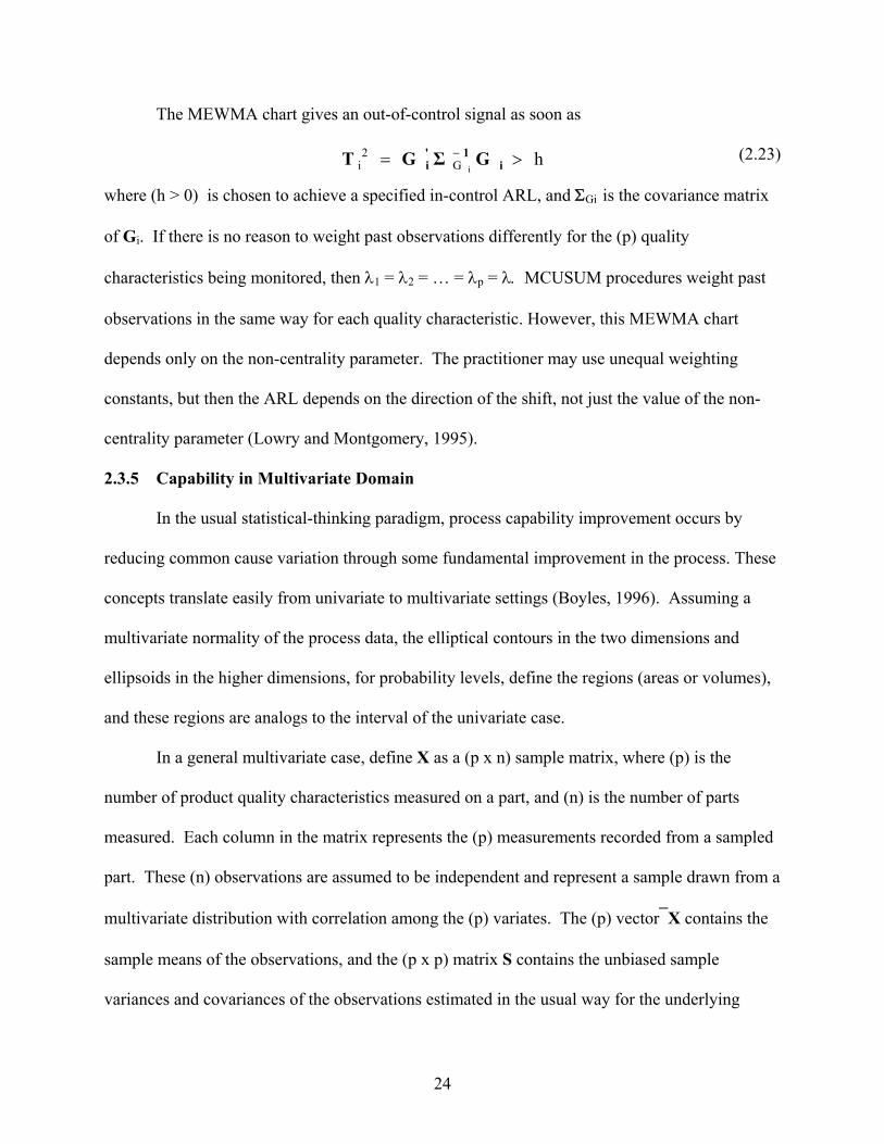
The MEWMA chart gives an out-of-control signal as soon as
(2.23)
where (h > 0) is chosen to achieve a specified in-control ARL, and ΣGi is the covariance matrix
of Gi. If there is no reason to weight past observations differently for the (p) quality
characteristics being monitored, then λ1 = λ2 = … = λp = λ. MCUSUM procedures weight past
observations in the same way for each quality characteristic. However, this MEWMA chart
depends only on the non-centrality parameter. The practitioner may use unequal weighting
constants, but then the ARL depends on the direction of the shift, not just the value of the non-
centrality parameter (Lowry and Montgomery, 1995).
2.3.5 Capability in Multivariate Domain
In the usual statistical-thinking paradigm, process capability improvement occurs by
reducing common cause variation through some fundamental improvement in the process. These
concepts translate easily from univariate to multivariate settings (Boyles, 1996). Assuming a
multivariate normality of the process data, the elliptical contours in the two dimensions and
ellipsoids in the higher dimensions, for probability levels, define the regions (areas or volumes),
and these regions are analogs to the interval of the univariate case.
In a general multivariate case, define X as a (p x n) sample matrix, where (p) is the
number of product quality characteristics measured on a part, and (n) is the number of parts
measured. Each column in the matrix represents the (p) measurements recorded from a sampled
part. These (n) observations are assumed to be independent and represent a sample drawn from a
multivariate distribution with correlation among the (p) variates. The (p) vector⎯X contains the
sample means of the observations, and the (p x p) matrix S contains the unbiased sample
variances and covariances of the observations estimated in the usual way for the underlying
hiG
2i >= −
i1'
i GΣGT
25
process mean μ0, and variance covariance matrix Σ. Engineering specifications are assumed to
exist for each of the (p) dimensions. The vector μ0 contains the target values for the (p) product
characteristics. In the multivariate domain, the objective is to use the X,⎯X , S, or the underlying
distribution in comparison to the engineering specifications to arrive at some acceptable
definition of capability in the multivariate domain (Wang et al., 2000).
A multivariate capability vector was proposed by Shahriari et al. (1995), based on the
original work of Hubele et al. (1991). The multivariate capability vector consists of three
components. Two components use the assumption that the process data is from a multivariate
normal distribution with elliptical contours defining the probability regions. The third component
is based on the geometric understanding of the process relative to the engineering specifications.
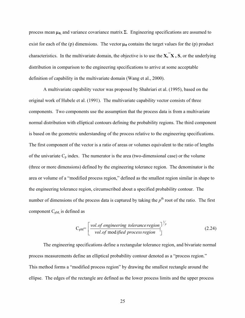
The first component of the vector is a ratio of areas or volumes equivalent to the ratio of lengths
of the univariate Cp index. The numerator is the area (two-dimensional case) or the volume
(three or more dimensions) defined by the engineering tolerance region. The denominator is the
area or volume of a “modified process region,” defined as the smallest region similar in shape to
the engineering tolerance region, circumscribed about a specified probability contour. The
number of dimensions of the process data is captured by taking the pth root of the ratio. The first
component CpM, is defined as
CpM= p
regionprocessifiedofvolregiontolerancegengineerinofvol
1
mod..
⎥⎦
⎤⎢⎣
⎡ (2.24)
The engineering specifications define a rectangular tolerance region, and bivariate normal
process measurements define an elliptical probability contour denoted as a “process region.”
This method forms a “modified process region” by drawing the smallest rectangle around the
ellipse. The edges of the rectangle are defined as the lower process limits and the upper process
26
limits (LPLi and UPLi, respectively, where i= 1, 2…, p) and are determined by solving the
system of equations of first derivatives, with respect to each xi, of the quadratic form
(X -μ0)′ Σ (X -μ0) = 2),p( αχ (2.25)
The distribution of the statistic follows a multivariate normal distribution. When the
process data is a multivariate normal, the distribution of the statistic will follow a χ2 distribution.
The two solutions to this equation for each dimension provide the upper and lower limits
UPLi = μi + )det(
)det(x1
1i
2),p(
−
−α
Σ
Σ (2.26)
LPLi = μi - )det(
)det(x1
1i
2),p(
−
−α
Σ
Σ (2.27)
where i=1, 2, …, p, and χ2(p,α) is the upper 100 ( )α percentile of a χ2 distribution with (p) degrees
of freedom associated with the probability contour and det (Σi-1) is the determinant of Σi
-1, a
matrix obtained from Σ -1 by deleting the ith row and column. Estimates from larger samples may
be used instead of μ and Σ (Johnson and Wichern, 1992).
The idea is to construct a modified process region with the same general geometric shape
as the engineering tolerance region. Thus,
CpM = ( )
p1
p
1iii
p
1iii
)LPLUPL(
LSLUSL
⎥⎥⎥⎥
⎦
⎤
⎢⎢⎢⎢
⎣
⎡
−
−
∏
∏
=
= (2.28)
To interpret the results, values higher than 1 indicate that the circumscribed modified
process region is smaller than the engineering specified region “goodness.” The limits UPL and
27
LPL are derived from the projection of probability ellipse onto the respective axes (Nickerson,
1994).
Also, when the engineering specifications are intervals and the product of the length of
the intervals forms the volume, then CpM could be calculated by multiplying univariate capacity
indices
CpM = ( )
( )p1
p
1i i
i
spreadprocessactualspreadprocessallowable
⎥⎦
⎤⎢⎣
⎡∏
= (2.29)
The second component of the vector is based on the assumption that the center of the
engineering specifications is the true underlying mean of the process. A Hotelling T2 statistic is
computed, and the second component is defined to be the significance level of the observed
value. That is,
T2 = n ( )′− 0μX S-1 ( )0μX − (2.30)
with the second component defined as
PV = P (T2 > pn
)1n(p−− F (p, n-p)) (2.31)
and PV is a probability value which never exceeds 1. A PV value closer to zero indicates that
the center of the process is “far” from the engineering target value.
The third component summarizes a comparison of the location of the modified process
region and the tolerance region (L1). It indicates whether any part of the modified process
region falls outside the engineering specifications. It has a binary value of (0, 1). L1 has the
value of 1 if the entire modified process region is contained within the tolerance region,
otherwise L1 = 0.
28
The three components [CpM, PV, L1] represent a comparison of the volumes of regions,
locations of centers, and location of regions. This multivariate index requires the assumption of
multivariate normality (Wang et al., 2000).
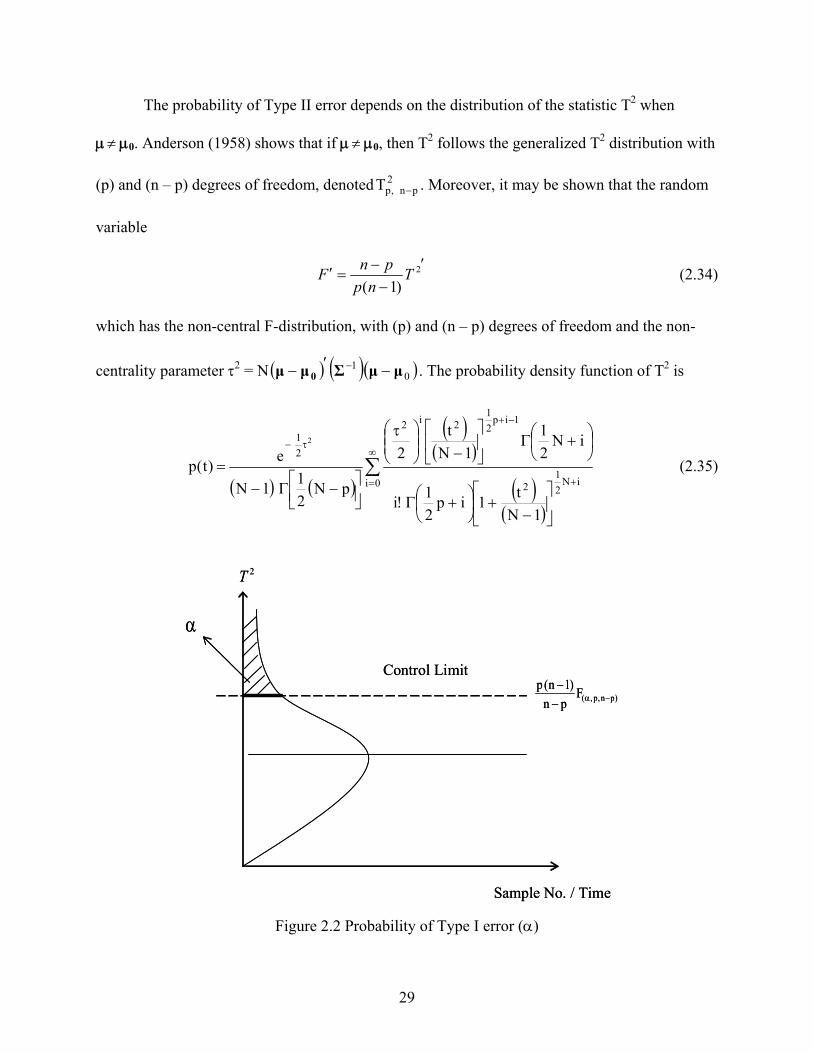
2.3.6 Statistical Performance
When comparing multivariate control schemes, a performance aspect should be
discussed. This aspect concerns the question of how quickly the scheme generates a signal when
an actual change in the process has occurred. The quicker a scheme responds to a real change,
the more advantageous. A control scheme that can quickly detect real changes while not being
overly sensitive to false alarm is desired. In particular, it is possible to identify two different
situations. With Type I error probability (α), or false positive, the control chart indicates an out-
of-control signal but the process is in-control. With Type II error probability (β), or false
negative, the control chart fails to indicate an out-of-control signal, while the process is out-of-
control. The number of samples required to detect a real change in the process is measured by
the run length. The expected value is then the average run length (ARL) (Montgomery, 2001).
Therefore, a good performance of a control scheme is obtained if the ARL is low in out-of-
control situations. As was pointed out in equation (2.1), ARL0 =α1 , where
⎥⎦⎤
⎢⎣⎡ =>= 0μμUCL2TPα (2.32)
and from equation (2.2), ARL1 = β−1
1 , where
⎥⎦⎤
⎢⎣⎡ ≠<= 0μμUCL2TPβ (2.33)
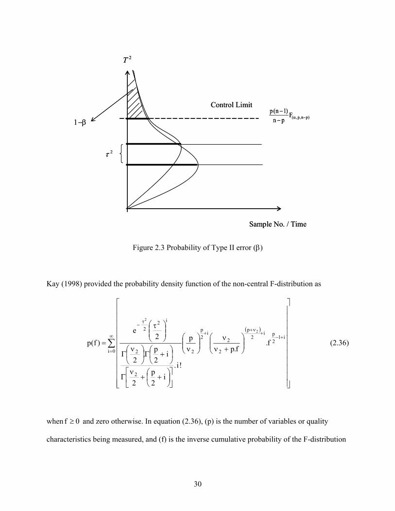
Figures 2.2 and 2.3 illustrate the probability of Type I and Type II errors respectively.
29
The probability of Type II error depends on the distribution of the statistic T2 when
μ ≠ μ0. Anderson (1958) shows that if μ ≠ μ0, then T2 follows the generalized T2 distribution with
(p) and (n – p) degrees of freedom, denoted 2pn,pT − . Moreover, it may be shown that the random
variable
′−
−=′ 2
)1(T
nppnF (2.34)
which has the non-central F-distribution, with (p) and (n – p) degrees of freedom and the non-
centrality parameter τ2 = N ( ) ( )( )01 μμΣμμ 0 −′− − . The probability density function of T2 is
( ) ( )
( )( )
( )( )
∑∞
= +
−+
τ−
⎥⎦
⎤⎢⎣
⎡
−+⎟
⎠⎞
⎜⎝⎛ +Γ
⎟⎠⎞
⎜⎝⎛ +Γ⎥
⎦
⎤⎢⎣
⎡
−⎟⎟⎠
⎞⎜⎜⎝
⎛ τ
⎥⎦⎤
⎢⎣⎡ −Γ−
=0i iN
21
2
1ip21
2i2
21
1Nt1ip
21!i
iN21
1Nt
2
pN211N
e)t(p
2
(2.35)
Figure 2.2 Probability of Type I error (α)
Sample No. / Time
Control Limit
α
2T
)pn,p,(Fpn
)1n(p−α−
−
Sample No. / Time
Control Limit
α
2T
)pn,p,(Fpn
)1n(p−α−
−
30
Figure 2.3 Probability of Type II error (β)
Kay (1998) provided the probability density function of the non-central F-distribution as
( )
∑∞
=
+−+
ν++
τ−
⎥⎥⎥⎥⎥⎥⎥⎥⎥⎥⎥
⎦
⎤
⎢⎢⎢⎢⎢⎢⎢⎢⎢⎢⎢
⎣
⎡
⎟⎟⎠
⎞⎜⎜⎝
⎛+ν
ν⎟⎟⎠
⎞⎜⎜⎝
⎛ν
⎥⎦
⎤⎢⎣
⎡⎟⎠⎞
⎜⎝⎛ ++
νΓ
⎟⎠⎞
⎜⎝⎛ +Γ⎟
⎠
⎞⎜⎝
⎛ νΓ
⎟⎟⎠
⎞⎜⎜⎝
⎛ τ
=0i
i12pi
2p
2
2i
2p
2
2
2
i22
f.f.p
p
!i.i
2p
2
i2p.
2
2e
)f(p2
2
(2.36)
when 0f ≥ and zero otherwise. In equation (2.36), (p) is the number of variables or quality
characteristics being measured, and (f) is the inverse cumulative probability of the F-distribution
Sample No. / Time
Control Limit
1−β
2τ
2T
)pn,p,(Fpn
)1n(p−α−
−
Sample No. / Time
Control Limit
1−β
2τ
2T
)pn,p,(Fpn
)1n(p−α−
−
31
F(1-α), p, ν2, with (p) and (ν2) degrees of freedom, where ν2 = (n – p + 1)/2. The degrees of freedom
are positive. When τ2 = 0, the non-central F-distribution becomes the F-distribution.
2.3.7 Advantages of Multivariate Statistical Process Control
Multivariate SPC has several advantages over univariate SPC. As noted by Hotelling,
(1947); Alt, (1984); and Lowry and Montgomery, (1995), multivariate SPC requires no
additional data accumulated for univariate control charts. Hotelling (1947) indicated that
multivariate SPC has the ability to combine measures in several dimensions into a single
measure of performance. In addition, multivariate SPC offers an easier graphical tool to
examine; the practitioner can only use one chart instead of multiple univariate charts to evaluate
the product or system quality as a whole rather than the sum of many individual parts (Hotelling,
1947, and Montgomery, 2001). Moreover, Montgomery (2001) demonstrated that multivariate
control charts will produce an acceptable Type I error or in-control run length while maintaining
the original data means, variances, and correlations. Multivariate statistics consider the
relationship between the variables since the variance-covariance matrix is part of the
computations (Hotelling, 1947). As such, multivariate control charts can detect changes in the
relationships among the variables being monitored, which would not be noticeable from separate
univariate charts (Lowry and Montgomery, 1995).
Another advantage is that multivariate SPC provides the appropriate control region for
the application. If the assumption of independence does not hold, then the assumed performance
of traditional Shewhart approaches can be misleading. The multivariate approach, however, can
guarantee error protection for a variety of different types of shifts in the process. Also, in the
multivariate domain, an advantage of the multivariate statistic is that it moves away from the
application of run rules (Sullivan and Woodall, 1996).

32
2.3.8 Disadvantages of Multivariate Statistical Process Control
While the literature provides strong evidence for the benefits of applying multivariate
SPC, a number of limitations were sited. As pointed out by Mason et al. (1997), Ryan (2000),
and Montgomery (2001), multivariate control charting procedures are computationally intensive.
Furthermore, multivariate control charts work well when the number of process variables is not
too large, i.e., (p > 10). As the number of variables grows, multivariate control charts lose
efficiency with regard to shift detection. Moreover, multivariate control chart procedures do not
directly provide the information an operator needs when the control chart signals an out-of-
control condition. It doesn’t provide information on which variable or set of variables is out-of-
control (Hawkins, 1991). Jackson and Mudholkar (1979) proposed the transformation of
correlated quality characteristic variables into a set of independent variables. Known as principle
component analysis (PCA), this approach reduces the dimensionality of the problem. In addition,
when applying Shewhart control charts, the use of averages of subgroups substantially improves
control chart performance. However, this is not always the case when using MCUSUM
(Montgomery, 2001).
2.4 Economic Models
Control charts have been used traditionally to establish and maintain statistical control of
a process. However, the design of a control chart has economic consequences, which are all
affected by the choice of the control chart parameters such as the selection of the sample size (n),
the width coefficient of the control limits (k), and the time interval between samples (h). Three
categories of costs are customarily considered in the economic design of control charts. These
categories are the cost of sampling and testing, the cost associated with investigating out-of-
33
control signals and correcting the assignable causes, and the costs of allowing nonconforming
units to reach the customer.
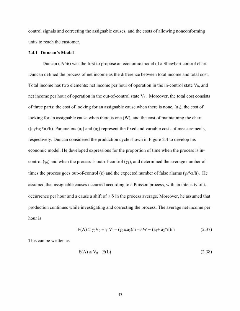
2.4.1 Duncan’s Model
Duncan (1956) was the first to propose an economic model of a Shewhart control chart.
Duncan defined the process of net income as the difference between total income and total cost.
Total income has two elements: net income per hour of operation in the in-control state V0, and
net income per hour of operation in the out-of-control state V1. Moreover, the total cost consists
of three parts: the cost of looking for an assignable cause when there is none, (a3), the cost of
looking for an assignable cause when there is one (W), and the cost of maintaining the chart
((a1+a2*n)/h). Parameters (a1) and (a2) represent the fixed and variable costs of measurements,
respectively. Duncan considered the production cycle shown in Figure 2.4 to develop his
economic model. He developed expressions for the proportion of time when the process is in-
control (γ0) and when the process is out-of-control (γ1), and determined the average number of
times the process goes out-of-control (ε) and the expected number of false alarms (γ0*α/h). He
assumed that assignable causes occurred according to a Poisson process, with an intensity of λ
occurrence per hour and a cause a shift of ± δ in the process average. Moreover, he assumed that
production continues while investigating and correcting the process. The average net income per
hour is
E(A) ≅ γ0V0 + γ1V1 – (γ0 αa3)/h – εW − (a1+ a2*n)/h (2.37)
This can be written as
E(A) ≅ V0 – E(L) (2.38)
34
The expression E(L) represents the expected loss per hour incurred by the process. E(L) is a
function of the control chart parameters (n), (k), and (h). Maximizing the expected net income
per hour V0 is equivalent to minimizing E(L).
Figure 2.4 Production cycle in Duncan’s model
Duncan incorporated formal optimization methodology into determining the control chart
parameters. Several numerical approximations were used in the structure and optimization of
this model. An optimization procedure was developed based on using a numerical approximation
to the system of first partial derivatives of E(L) with respect to (n), (k), and (h). Duncan
compared the optimum design with the heuristic design of n = 5, k = 3, and h = 1 for a set of 25
examples at different levels of input parameters. He concluded that using the heuristic design in
some cases might result in vary large penalties.
Duncan’s research was the stimulus for much of the research that followed in this area.
Several interventions were conducted to investigate further optimization methods, model
sensitivity, and its application to other Shewhart control charts.
Production Cycle
In-Control
Time to Signal Find & Fix Sample & Test
Out-of-Control
Shift OccursStart End
35
Alexander et al. (1995) embellished Duncan’s cause model with the Taguchi loss
function that defines losses owing to the variability caused by both chance and assignable causes.
Through sensitivity analysis, they indicated that the design parameters for the⎯x chart are fairly
robust when the cost of finding assignable cause and the frequency of occurrence of an
assignable cause are not very high. They found that (n) increases and (h) decreases to steady-
state values as the frequency of the process shift decreases. Moreover, they stated that the rate of
convergence to the steady-state depends on the cost of searching for an assignable cause.
Therefore, the higher the cost, the slower the convergence rate. Also, they indicated that (n) and
(h) must be adjusted based on the size of the process shift that is investigated. Therefore, small
process shifts require large values of (n) and (h), while for large process shifts, small (n) and (h)
values are recommended.
2.4.2 Lorenzen and Vance’s Model
In 1986, Lorenzen and Vance developed an economic model for the design of control
charts. They used a different approach in developing their model. Instead of using the Type I
error probability (α) and Type II error probability (β) risks, they based their approach on
developing their model on the in-control and out-of-control average run lengths. They considered
the production cycle shown in Figure 2.5. Moreover, they developed expressions for estimating
the in-control and out-of-control expected times. They considered the following costs in their
model: (1) cost incurred during the in-control period due to process sampling (a1+a2.n), where
nonconforming units produced C0, and False alarms Y; (2) cost incurred during the out-of-
control period, including the cost of nonconforming units that produced C0 and (C1>C0); and (3)
cost of locating and repairing the assignable cause (W) and that of process sampling. The total
cost per production cycle E(C) was
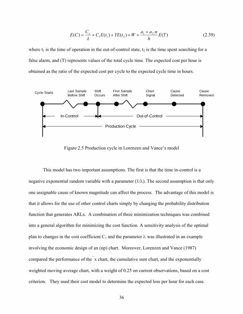
36
)(.)()()( 21211 TE
hnaaWtYEtEC
CCE o +
++++=λ
(2.39)
where t1 is the time of operation in the out-of-control state, t2 is the time spent searching for a
false alarm, and (T) represents values of the total cycle time. The expected cost per hour is
obtained as the ratio of the expected cost per cycle to the expected cycle time in hours.
Figure 2.5 Production cycle in Lorenzen and Vance’s model
This model has two important assumptions. The first is that the time in-control is a
negative exponential random variable with a parameter (1/λ). The second assumption is that only
one assignable cause of known magnitude can affect the process. The advantage of this model is
that it allows for the use of other control charts simply by changing the probability distribution
function that generates ARLs. A combination of three minimization techniques was combined
into a general algorithm for minimizing the cost function. A sensitivity analysis of the optimal
plan to changes in the cost coefficient C1 and the parameter λ was illustrated in an example
involving the economic design of an (np) chart. Moreover, Lorenzen and Vance (1987)
compared the performance of the⎯x chart, the cumulative sum chart, and the exponentially
weighted moving average chart, with a weight of 0.25 on current observations, based on a cost
criterion. They used their cost model to determine the expected loss per hour for each case.
Production Cycle
Out-of-ControlIn-Control
Cause Removed
Cause Detected
Chart Signal
First Sample After Shift
Shift Occurs
Last Sample Before Shift
Cycle Starts
Production Cycle
Out-of-ControlIn-Control
Cause Removed
Cause Detected
Chart Signal
First Sample After Shift
Shift Occurs
Last Sample Before Shift
Cycle Starts
37
They assumed that manufacturing activities are allowed during investigating and repairing the
assignable cause. Their findings were that the CUSUM chart performed best, followed by the⎯x
chart, and then the EWMA chart.
2.4.3 Knappenberger and Grandage’s Model
Knappenberger and Grandage (1969) developed a model for the economic design of
the⎯x control charts. Their model was different than Duncan’s model in that there is no
constraint on the number of assignable causes that can occur. Specifically, the process can shift
from one out-of-control state to another, as long as the shift results in further quality
deterioration. It is assumed that the process is stopped while out-of-control signals are
investigated and that the costs of investigating both real and false alarms are the same. The
expected total cost E(C) per unit of product consists of three elements. The first element E(C1),
the expected cost per unit associated with carrying out the charting procedure is ((a1+a2.n)/k),
where k is the number of units produced between samples. The second element E(C2), the
expected cost per unit associated with investigating and correcting the process, when the chart
indicates the process is out-of-control, assuming that the process is stopped, is ((a3/k) q αt),
where q is a row vector representing values of probabilities qi (the probability of rejecting H0
when μ = μi, (i= 0, 1, 2, 3, 4, 5, 6)) and αt is the transpose of the row vector representing the
steady-state probability that the process is in state (i) (that is, μ = μi) at the time of the test. And
the third element E(C3), the expected unit of producing a defective product, is (a4φ γt), where (a4)
is the cost of a defective unit, φ is a row vector of the conditional probabilities of producing a
defective unit given the process mean, and γt is the transpose of the row vector representing the
true state of the process. Therefore, the sum of the three cost elements represents the expected
total cost per unit as
38
E(C) = E(C1) + E(C2) + E(C3) (2.40)
This can be written as
E (C) = (a1+a2.n)/k + (a3/k) qαt + a4φγt (2.41)
Knappenberger and Grandage used two-stage direct search method to minimize the cost
function. They conducted limited sensitivity analysis and presented the solutions to 81 numerical
examples of a variety of cost coefficients and process parameters. They also minimized the
expected cost per unit produced rather than the expected cost per unit time, as in Duncan’s
model.
2.4.3.1 Montgomery and Klatt’s Approach to Multivariate T2 Chart
Montgomery and Klatt (1972) developed an optimal economic design of the T2 control
chart. Based on the structure of the Knappenberger and Grandage model, they employed a single
assignable cause version. However, their results were restricted to the case of two quality
characteristics. It is assumed that, when μ = μ0, the process is in-control and there is only one
out-of-control state, which is when the process mean vector is μ1 = μ0 + δ, where the (p x 1)
vector δ is known. It is also assumed that the time the process remains in the in-control state
before going out-of-control is an exponential random variable with mean λ-1 hours. Moreover,
when the process goes out-of-control, it stays out-of-control until detected. However, the
assignable cause is detected as soon as the T2 chart plots out-of-control, that is, when
2,,
2pnpTT −> α . The expected total cost per unit of product E(C) consists of three terms. The first
term E(C1), the expected cost per unit of sampling and for carrying out the test procedure, is
((a1+a2.n)/k), where (a1) is the fixed cost per sample, (a2) is the per-unit cost of sampling, and (k)
is the number of units produced between successive samples. The second term E(C2) the
39
expected cost per unit of investigating and for correcting the process, is ((a3/k) β ρt), where (a3)
is the expected cost of investigating and correcting an out-of-control process. However, the cost
of investigating real and false alarms is assumed to be the same. Also, β is a column vector of the
probability that the process is in state μi (i = 0, 1) at the time the test is performed. The transpose
of the row vector of conditional probability is that the test procedure indicates the process is out-
of-control, given that the process is in state μi is ρt. The third element E(C3), the expected cost
per unit of producing a defective product, is (a4 γ φt), where (a4) is the cost of a defective unit, φ
is a column vector of the conditional probabilities of producing a defective unit given that μ = μi
process mean, and γ is the column vector of probability that the process is in state μi at any point
in time. Therefore, the sum of the three cost elements represents the expected total cost per unit
E(C) = E(C1) + E(C2) + E(C3), or
E(C) = (a1+a2.n)/k + (a3/k)βρt + a4.γφt (2.42)
Montgomery and Klatt also investigated the sensitivity of the model to estimates of the
cost coefficients and of the population covariance matrix. They concluded that the optimum
control chart parameters are relatively insensitive to errors in estimating these parameters. They
also concluded that both the magnitude of the shift and the sign (+/-) of the correlation
coefficient relating the two quality characteristics affect the optimum economic design.
Moreover, if the shift in both quality characteristics is in the same direction, negative correlation
between the quality characteristics leads to a smaller sample than would be required if the
correlation were positive. This occurs because negative correlation always leads to a more
powerful test if the process shift is in the same direction for both quality characteristics.
40
CHAPTER 3
DISCUSSION
In multivariate SPC, the focus usually is to simultaneously monitor several quality
characteristics that may be correlated. Hotelling first publicized the multivariate approach to
quality control in 1947 in the testing of bombsights. Hotelling introduced the T2 control chart as
a technique for monitoring the overall quality of a process. An advantage of this approach is that
the T2 statistic is a single measure of excellence. This field remained relatively undeveloped until
the late 1950’s with the increasing availability of computers.
Advancements in technology raised the need for simultaneous monitoring of several
quality characteristics that could be correlated. With increased competition in the marketplace,
many companies have utilized Six Sigma methodology as a means to reduce the cost of poor
quality in order to maintain their market share. The need to apply multivariate SPC became
more desirable, especially with the complexity of processes and the dependency of quality
characteristics on each other. Furthermore, customer expectations require the evaluation of the
product or system quality as a whole rather than the sum of many individual parts. With the
availability of product alternatives, customers are becoming more demanding for higher quality.
In order for companies to remain competitive, they must achieve high levels of product quality,
which is becoming challenging to achieve since quality characteristics are interrelated to each
other as a result of technological advancements. Additionally, management demand for
implementing Six Sigma programs to achieve better quality makes it more challenging to do so.
Recently this effort has made multivariate SPC more popular.
Practitioners in industry avoid using multivariate SPC because of its complex
computational intensiveness. However, increased availability of high-speed computers and
41
statistical software programs, formerly available only to very few, has made the statistical
computations of multivariate SPC easier.
Many new techniques have made multivariate SPC more useful (e.g., Ghare and
Torgerson, (1968); Montgomery and Wadsworth, (1972); Alt, (1973, 1982); Alt et al., (1976);
Montgomery and Klatt, (1972); Jackson, (1956, 1959); Jackson and Bradley, (1966); Jackson,
(1985); Tracy et al., (1992); Mason et al., (1997); and Woodall et al., (2004)). Among industries,
the use of multivariate control charts to monitor manufacturing processes is increasingly popular.
This is the result of many recent advances that have occurred in multivariate SPC, such as in
multivariate cumulative sum control charts (e.g., Crosier, (1988); Healy, (1987); Pignatiello and
Runger, (1990); Woodall and Ncube, (1985)); and multivariate exponentially weighted moving
average control charts (e.g, Lowry et al., 1992). The improved effectiveness of these techniques
has made it possible to identify the cause of an out-of-control signal. While it is common in
industry to monitor individual process characteristics with separate univariate charts, more
attention is being given to combine characteristics into a single chart.
Multivariate control charts are generally utilized in cases where the quality measurements
follow the multivariate normal distribution, and the process performance is monitored over time.
In addition, they can be used to indicate when quality characteristics change. In univariate SPC,
a signal is produced when a sample point does not confirm to the structure that is established by
the historical data. Through the use of appropriate control charts, it is possible to determine if
this signal is due to a shift in the process mean and/or a shift in the process variation. Since there
is only a single variable to consider, signal interpretation is relatively straightforward. However,
in multivariate SPC, a signal can be caused by a variety of situations. These include out-of-
control behavior of a single variable, a relationship between two or more variables, or a
42
combination of the two situations with some variables being out-of-control and others having a
counter-relationship due to the correlation between variables.
Multivariate SPC may be useful whenever there is more than one variable quantifying the
quality characteristic of a product and/or process. Multivariate SPC is particularly valuable
when these variables are correlated. In some cases, the true source of variation may not be
recognized or may not be measurable. Multivariate SPC is more resilient to correlation whether
it exists or not. Moreover, practitioners’ lack of knowledge of the correlation between the
quality characteristics in their processes does not mean that the correlation does not exist. It is
important to recognize that almost all processes are multivariate, but multivariate SPC often is
not utilized because the process characteristics are assumed to be independent. As a result
practitioners tend to use traditional SPC as an alternative to multivariate SPC. However, the
distortion in the process-monitoring procedure increases as the number of quality characteristic
increases since some of these variables may be correlated. Consequently, the more variables
there are, the more likely one of the charts will contain an out-of-control condition, even when
the process has not shifted. Thus, the false alarm rate or probability of Type 1 error is increased
if each variable is controlled separately.
Multivariate control charting provides a means to identifying shifts in any (p) quality
characteristics by charting only one parameter such as Hotelling T2. This simplifies the charting
procedures. It is easier to monitor one chart rather than monitoring several charts for the same
quality characteristics. Moreover, industries are determined to achieve higher levels of product
and process quality with the least amount of resources committed. Multivariate SPC reduces the
cost of process monitoring since it works with the same data collected for traditional SPC.
43
The increasing demand for less variability raises the need to monitor correlated variables
simultaneously. A number of methodologies were developed to provide a clear procedure for
interpreting out-of-control signals in the case of multivariate control charts. However, limited
research has been conducted to address their implementation boundaries and utilization in
practice.
A literature review of multivariate control charts was presented in Chapter 2. The
literature did not provide specific guidelines of when to use multivariate statistical analysis.
Industry applications require practitioners to be able to decide when it is necessary to use
multivariate control charts. An important implication of this is the need for practitioners to know
the level of correlation of process characteristics and the process model parameters in order to
decide when to use multivariate control charts to detect the special causes and interpret out-of-
control conditions.
3.1 Research Gap
Statistical process control has helped industry become more aware of the benefits of
implanting statistical procedures. Companies’ management requires their practitioners to use the
Six Sigma methodology as a method to reducing cost. Recent development in technology has
presented systems of interconnected processes. The key to the success is to understand and
reduce process variation. With the recent technological advancements, almost all processes are
related or dependent on common variables. Incidentally, quality practitioners often do not
investigate the correlation levels between the variables they are monitoring. Their
underestimation of the relationship between the variables will result in traditional SPC becoming
less effective. Most quality practitioners use Shewhart charts to monitor process performance
over time. Montgomery (2001) pointed out that if the (p) quality characteristics are not
44
independent, which is usually the case if they are related to the same product, then Type I and
Type II error probabilities for the traditional Shewhart charts become distorted. The literature
did not show any method for measuring the distortion in a Shewhart joint control procedure.
Additionally, there is a clear gap in the literature in indicating the levels of correlation that
mandate the use of multivariate charts. The statistical effect of mis-specifying the process model
while applying traditional Shewhart charts has not been quantified. The need to use multivariate
SPC has received great attention in recent years as companies strive to be more competitive and
achieve higher quality products with the lowest cost possible.
Companies are becoming more customer-focused and need to remain competitive; this
makes it economically necessary to utilize the best SPC techniques. The economic consequences
of using Shewhart charts as a preference procedure to multivariate charts were not presented in
the literature. Practitioners need to be aware of the most economical SPC method in order to
monitor the performance of the quality characteristics of any process.
3.2 Research Objectives
This research addressed the gap identified in section 3.1, based on the literature review.
This was accomplished by quantifying the effect of changes in the level of correlation between
variables coupled with changes in the process model and chart design parameters. Another
objective was to assess the economic feasibility of utilizing Hotelling’s T2 multivariate control
chart as an alternative to traditional Shewhart⎯x charts. This investigation was undertaken for the
case of two quality characteristics.
Special considerations were given to the Hotelling T2 chart. As such, the most popular
Shewhart⎯x chart was used to provide a baseline for the performance measures. Measures of
performance were selected to evaluate the statistical performance and economic feasibility for
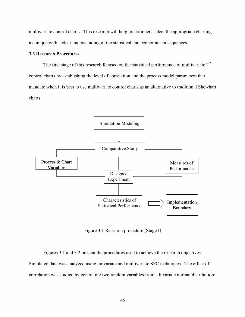
45
multivariate control charts. This research will help practitioners select the appropriate charting
technique with a clear understanding of the statistical and economic consequences.
3.3 Research Procedures
The first stage of this research focused on the statistical performance of multivariate T2
control charts by establishing the level of correlation and the process model parameters that
mandate when it is best to use multivariate control charts as an alternative to traditional Shewhart
charts.
Figure 3.1 Research procedure (Stage I)
Figures 3.1 and 3.2 present the procedures used to achieve the research objectives.
Simulated data was analyzed using univariate and multivariate SPC techniques. The effect of
correlation was studied by generating two random variables from a bivariate normal distribution;
Process & Chart Variables
Measures of Performance
Designed Experiment
Characteristics of Statistical Performance
Implementation Boundary
Simulation Modeling
Comparative Study
Process & Chart Variables
Measures of Performance
Designed Experiment
Characteristics of Statistical Performance
Implementation Boundary
Simulation Modeling
Comparative Study
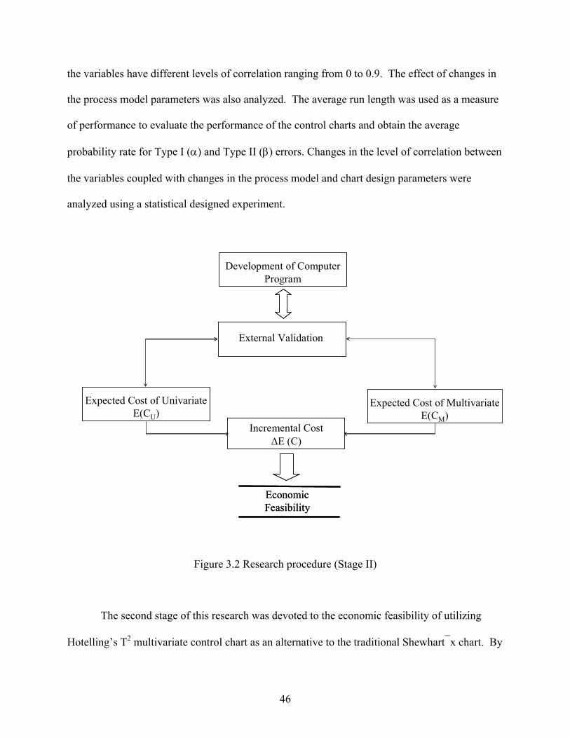
46
the variables have different levels of correlation ranging from 0 to 0.9. The effect of changes in
the process model parameters was also analyzed. The average run length was used as a measure
of performance to evaluate the performance of the control charts and obtain the average
probability rate for Type I (α) and Type II (β) errors. Changes in the level of correlation between
the variables coupled with changes in the process model and chart design parameters were
analyzed using a statistical designed experiment.
Figure 3.2 Research procedure (Stage II)
The second stage of this research was devoted to the economic feasibility of utilizing
Hotelling’s T2 multivariate control chart as an alternative to the traditional Shewhart⎯x chart. By
Incremental CostΔE (C)
Economic Feasibility
Expected Cost of UnivariateE(CU)
Expected Cost of MultivariateE(CM)
Development of Computer Program
External Validation
Incremental CostΔE (C)
Economic Feasibility
Expected Cost of UnivariateE(CU)
Expected Cost of MultivariateE(CM)
Development of Computer Program
External Validation

47
using economic design models from Knappenberger and Grandage (1969), and Montgomery and
Klatt (1972) for the traditional Shewhart⎯x chart and the multivariate T2 chart respectively, an
incremental cost model was constructed to examine the cost and worth of switching from
univariate to multivariate SPC techniques under specified levels of process and chart variables,
thus determining the economic consequences of using traditional Shewhart charts.
48
CHAPTER 4
INITIAL INVESTIGATIONS
To determine the characteristics of statistical performance of the Shewhart⎯x and
multivariate T2 charts, initial investigations of the charts performance were conducted to account
for the Type I probability (α) and Type II probability (β) errors. Simulation modeling was
developed and verified using operating characteristics (OC) curves for the Shewhart⎯x chart. The
performance of the multivariate T2 chart was validated using the same conditions of the
Shewhart⎯x chart under (0) correlation conditions. After this process was done, the simulation
was carried out to calculate Type I probability (α) and Type II probability (β) errors for the two
SPC techniques.
Random variables were generated at specified levels of correlation ranging from (– 0.8)
to (+ 0.8). Simulated data were analyzed using univariate and multivariate SPC techniques to
study the average rate of false alarms based on simulated ARL0. After causing a shift in the
mean, ranging from 1σ to 3 σ, simulated data were analyzed to study the probability of Type II
error following the shift based on simulated ARL1.
4.1 Simulation Development and Verification
A simulation was conducted using the software @ RiskTM version 4, an add-in for
Microsoft Excel software, to generate simulated data of two random variables from bivariate
normal distribution using a random generating function. The levels of correlation between the
two variables were then varied over a range from (- 0.8) to (+ 0.8). Equation (2.1) provides the
expected value of ARL0 for the⎯x chart with 3 σ limits as
4.3700027.011)x(EARL0 ==
α==
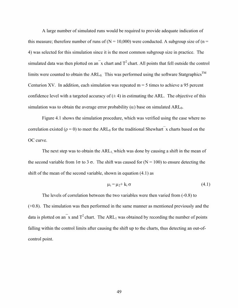
49
A large number of simulated runs would be required to provide adequate indication of
this measure; therefore number of runs of (N = 10,000) were conducted. A subgroup size of (n =
4) was selected for this simulation since it is the most common subgroup size in practice. The
simulated data was then plotted on an⎯x chart and T2 chart. All points that fell outside the control
limits were counted to obtain the ARL0. This was performed using the software StatgraphicsTM
Centurion XV. In addition, each simulation was repeated m = 5 times to achieve a 95 percent
confidence level with a targeted accuracy of (± 4) in estimating the ARL. The objective of this
simulation was to obtain the average error probability (α) base on simulated ARL0.
Figure 4.1 shows the simulation procedure, which was verified using the case where no
correlation existed (ρ = 0) to meet the ARL0 for the traditional Shewhart⎯x charts based on the
OC curve.
The next step was to obtain the ARL1, which was done by causing a shift in the mean of
the second variable from 1σ to 3 σ. The shift was caused for (N = 100) to ensure detecting the
shift of the mean of the second variable, shown in equation (4.1) as
μi = μ2+ ki σ (4.1)
The levels of correlation between the two variables were then varied from (-0.8) to
(+0.8). The simulation was then performed in the same manner as mentioned previously and the
data is plotted on an⎯x and T2 chart. The ARL1 was obtained by recording the number of points
falling within the control limits after causing the shift up to the charts, thus detecting an out-of-
control point.
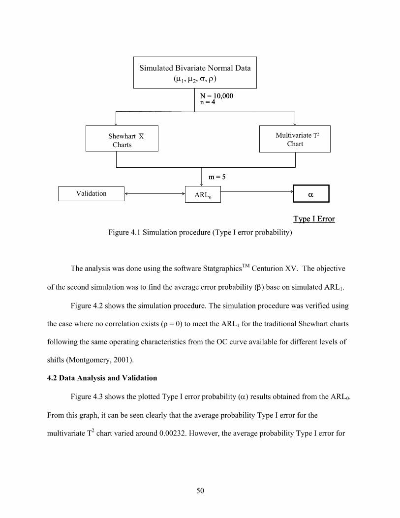
50
Figure 4.1 Simulation procedure (Type I error probability)
The analysis was done using the software StatgraphicsTM Centurion XV. The objective
of the second simulation was to find the average error probability (β) base on simulated ARL1.
Figure 4.2 shows the simulation procedure. The simulation procedure was verified using
the case where no correlation exists (ρ = 0) to meet the ARL1 for the traditional Shewhart charts
following the same operating characteristics from the OC curve available for different levels of
shifts (Montgomery, 2001).
4.2 Data Analysis and Validation
Figure 4.3 shows the plotted Type I error probability (α) results obtained from the ARL0.
From this graph, it can be seen clearly that the average probability Type I error for the
multivariate T2 chart varied around 0.00232. However, the average probability Type I error for
Simulated Bivariate Normal Data(μ1, μ2, σ, ρ)
ARL0
Multivariate T2
Chart
α
N = 10,000n = 4
m = 5
Shewhart Charts
X
Type I Error
Validation
Simulated Bivariate Normal Data(μ1, μ2, σ, ρ)
ARL0
Multivariate T2
Chart
α
N = 10,000n = 4
m = 5
Shewhart Charts
X
Type I Error
Validation
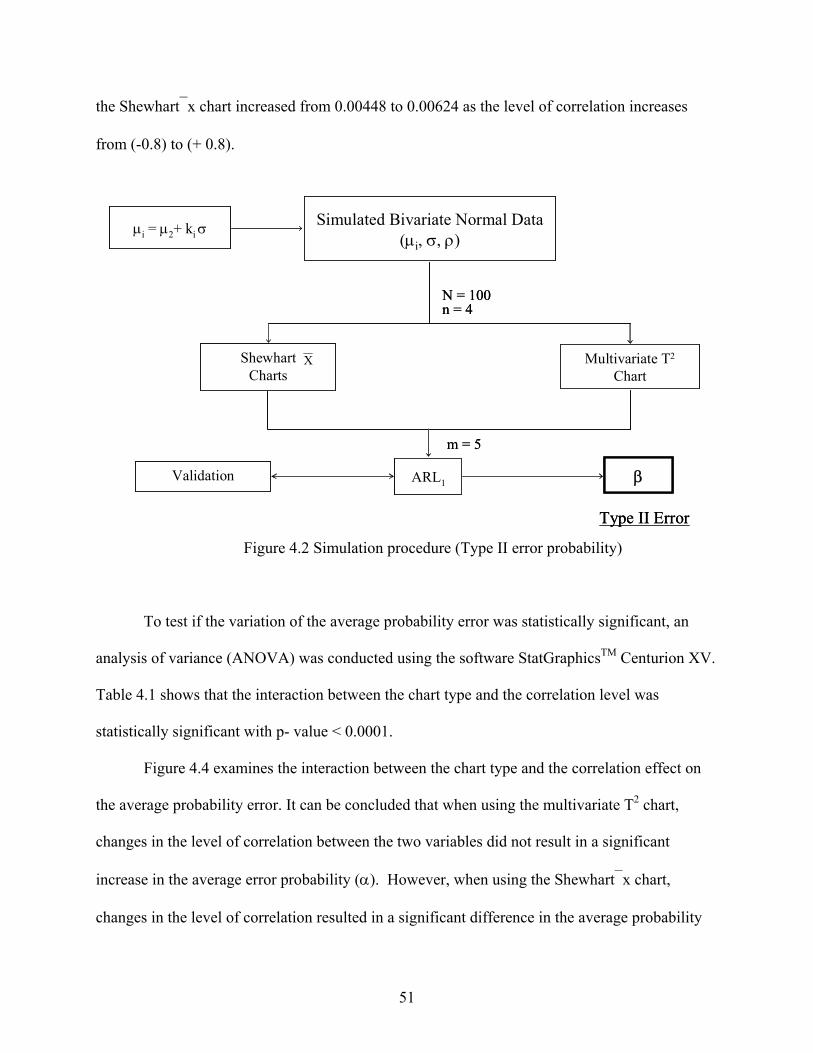
51
the Shewhart⎯x chart increased from 0.00448 to 0.00624 as the level of correlation increases
from (-0.8) to (+ 0.8).
Figure 4.2 Simulation procedure (Type II error probability)
To test if the variation of the average probability error was statistically significant, an
analysis of variance (ANOVA) was conducted using the software StatGraphicsTM Centurion XV.
Table 4.1 shows that the interaction between the chart type and the correlation level was
statistically significant with p- value < 0.0001.
Figure 4.4 examines the interaction between the chart type and the correlation effect on
the average probability error. It can be concluded that when using the multivariate T2 chart,
changes in the level of correlation between the two variables did not result in a significant
increase in the average error probability (α). However, when using the Shewhart⎯x chart,
changes in the level of correlation resulted in a significant difference in the average probability
Type II Error
ARL1
μi = μ2+ ki σ
β
Shewhart Charts
Multivariate T2
Chart
N = 100n = 4
m = 5
X
Simulated Bivariate Normal Data(μi, σ, ρ)
Validation
Type II Error
ARL1
μi = μ2+ ki σ
β
Shewhart Charts
Multivariate T2
Chart
N = 100n = 4
m = 5
X
Simulated Bivariate Normal Data(μi, σ, ρ)
Validation
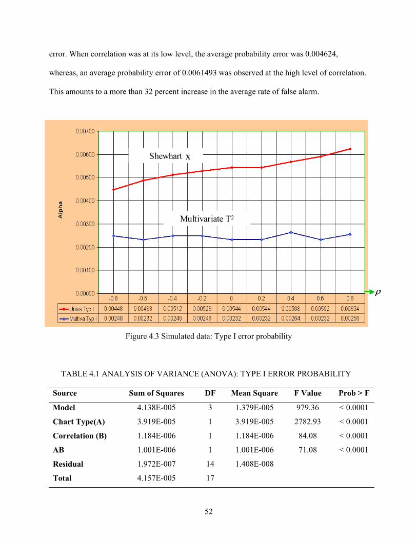
52
error. When correlation was at its low level, the average probability error was 0.004624,
whereas, an average probability error of 0.0061493 was observed at the high level of correlation.
This amounts to a more than 32 percent increase in the average rate of false alarm.
Figure 4.3 Simulated data: Type I error probability
TABLE 4.1 ANALYSIS OF VARIANCE (ANOVA): TYPE I ERROR PROBABILITY
Source Sum of Squares DF Mean Square F Value Prob > F
Model 4.138E-005 3 1.379E-005 979.36 < 0.0001
Chart Type(A) 3.919E-005 1 3.919E-005 2782.93 < 0.0001
Correlation (B) 1.184E-006 1 1.184E-006 84.08 < 0.0001
AB 1.001E-006 1 1.001E-006 71.08 < 0.0001
Residual 1.972E-007 14 1.408E-008
Total 4.157E-005 17
ρ
Shewhart
Multivariate T2
x
ρ
Shewhart
Multivariate T2
x
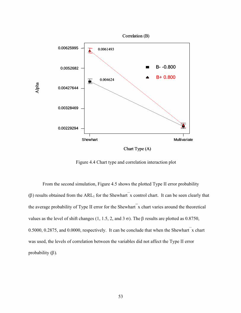
53
Figure 4.4 Chart type and correlation interaction plot
From the second simulation, Figure 4.5 shows the plotted Type II error probability
(β) results obtained from the ARL1 for the Shewhart⎯x control chart. It can be seen clearly that
the average probability of Type II error for the Shewhart⎯x chart varies around the theoretical
values as the level of shift changes (1, 1.5, 2, and 3 σ). The β results are plotted as 0.8750,
0.5000, 0.2875, and 0.0000, respectively. It can be conclude that when the Shewhart⎯x chart
was used, the levels of correlation between the variables did not affect the Type II error
probability (β).
B- -0.800
B+ 0.800
Correlation (B)
Chart Type (A)
Alp
ha
Shewhart Multivariate
0.00229294
0.00328469
0.00427644
0.0052682
0.00625995 0.0061493
0.004624
B- -0.800
B+ 0.800
Correlation (B)
Chart Type (A)
Alp
ha
Shewhart Multivariate
0.00229294
0.00328469
0.00427644
0.0052682
0.00625995 0.0061493
0.004624
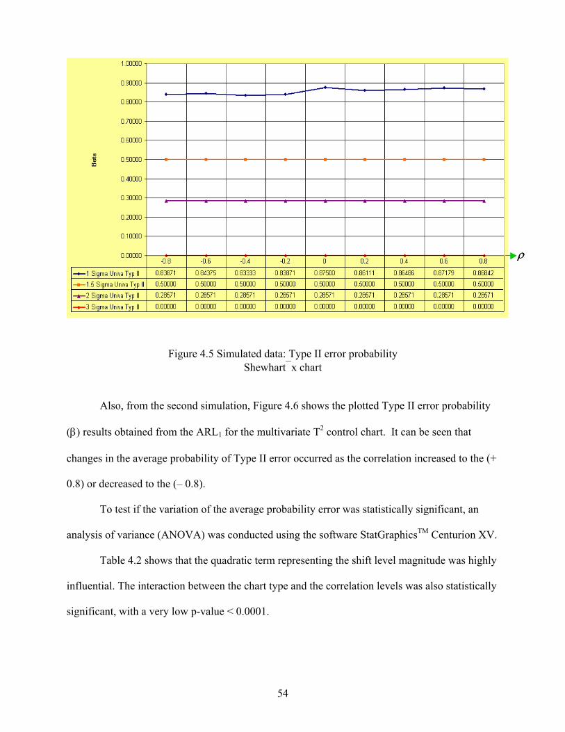
54
Figure 4.5 Simulated data: Type II error probability Shewhart⎯x chart
Also, from the second simulation, Figure 4.6 shows the plotted Type II error probability
(β) results obtained from the ARL1 for the multivariate T2 control chart. It can be seen that
changes in the average probability of Type II error occurred as the correlation increased to the (+
0.8) or decreased to the (– 0.8).
To test if the variation of the average probability error was statistically significant, an
analysis of variance (ANOVA) was conducted using the software StatGraphicsTM Centurion XV.
Table 4.2 shows that the quadratic term representing the shift level magnitude was highly
influential. The interaction between the chart type and the correlation levels was also statistically
significant, with a very low p-value < 0.0001.
ρρ

55
Figure 4.6 Simulated data: Type II error probability multivariate T2 chart
TABLE 4.2 ANALYSIS OF VARIANCE (ANOVA): TYPE II ERROR PROBABILITY
Source Sum of Squares DF Mean Square F Value Prob > F
Model 2.5 6 0.34 163.75 < 0.0001
Chart Type(A) 0.14 1 0.14 67.53 < 0.0001
Correlation (B) 0.14 1 0.14 67.77 < 0.0001
Shift Level (C) 1.56 1 1.56 748.24 < 0.0001
B2 0.012 1 0.012 5.71 < 0.0255
C2 0.054 1 0.54 25.70 < 0.0001
AB 0.14 1 0.14 67.54 < 0.0001
Residual 0.048 23 2.086E-003
Total 2.10 29
ρρρ
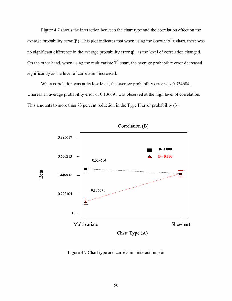
56
Figure 4.7 shows the interaction between the chart type and the correlation effect on the
average probability error (β). This plot indicates that when using the Shewhart⎯x chart, there was
no significant difference in the average probability error (β) as the level of correlation changed.
On the other hand, when using the multivariate T2 chart, the average probability error decreased
significantly as the level of correlation increased.
When correlation was at its low level, the average probability error was 0.524684,
whereas an average probability error of 0.136691 was observed at the high level of correlation.
This amounts to more than 73 percent reduction in the Type II error probability (β).
Figure 4.7 Chart type and correlation interaction plot
B- 0.000
B+ 0.800
Correlation (B)
Chart Type (A)
Bet
a
Multivariate Shewhart
0
0.223404
0.446809
0.670213
0.893617
0.524684
0.136691
B- 0.000
B+ 0.800
Correlation (B)
Chart Type (A)
Bet
a
Multivariate Shewhart
0
0.223404
0.446809
0.670213
0.893617
0.524684
0.136691

57
As a result of the initial investigation, a strong relationship between chart type and
correlation levels was detected. Further in-depth investigation is required in order to characterize
the statistical performance of the Shewhart⎯x and the multivariate T2 charts and identify any
thresholds of the process and chart variables. Chapter 5 provides a designed experiment to
conduct this exploration, using data that was generated utilizing the same simulation procedure.
The simulation was verified and validated based on the OC curves of the Shewhart⎯x for the case
of no correlation (ρ = 0).
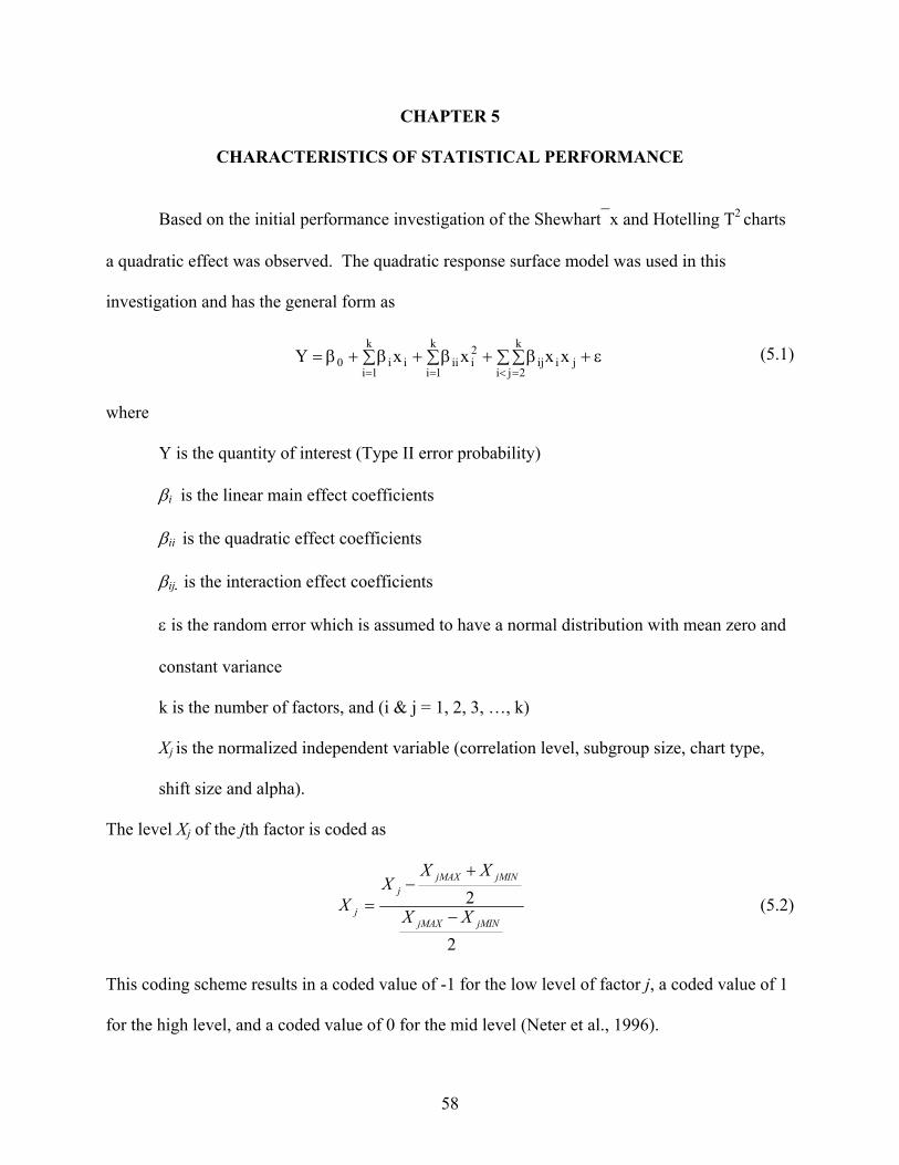
58
CHAPTER 5
CHARACTERISTICS OF STATISTICAL PERFORMANCE
Based on the initial performance investigation of the Shewhart⎯x and Hotelling T2 charts
a quadratic effect was observed. The quadratic response surface model was used in this
investigation and has the general form as
ε+∑ ∑β+∑β+∑β+β=< === ji
jk
2iij
2i
k
1iii
k
1iii0 xxxxY (5.1)
where
Y is the quantity of interest (Type II error probability)
βi is the linear main effect coefficients
βii is the quadratic effect coefficients
βij is the interaction effect coefficients
ε is the random error which is assumed to have a normal distribution with mean zero and
constant variance
k is the number of factors, and (i & j = 1, 2, 3, …, k)
Xj is the normalized independent variable (correlation level, subgroup size, chart type,
shift size and alpha).
The level Xj of the jth factor is coded as
2
2jMINjMAX
jMINjMAXj
j XX
XXX
X−
+−
= (5.2)
This coding scheme results in a coded value of -1 for the low level of factor j, a coded value of 1
for the high level, and a coded value of 0 for the mid level (Neter et al., 1996).

59
5.1 Design Selection
When designing a response surface study, a minimal requirement is that the design must
be capable of providing estimates of the p = (k+1)(k+2)/2 parameters in the model. Any design
of resolution V or higher for a two-level factorial study will provide estimates of linear main
effect and all two-factor interaction effects that are confounded only with higher-order effects.
However, at least three levels of each factor must be presented to obtain estimates of the k
quadratic main effects.
One design that provides estimates of all parameters in the regression model shown in
equation (5.1) is the full factorial design with each factor at three levels (3k). A number of
limitations are associated with this design. First, the number of treatments required by a 3k grows
rapidly with the number of factors. Second, each factor appears at exactly three levels so that it
will not be possible to test for the presence of cubic or higher-order main effects (Myers and
Montgomery, 2002).
A central composite design (CCD) of two-level full factorial 2k was chosen in this study
to examine the effect of changes in the level of correlation between variables coupled with
changes in the process model and chart design variables for the Type II error probability. This
design allows assigning a small number of carefully chosen treatments to permit estimation of
the second-order response surface model.
Characteristics of CCD depend on the choice of the number of numeric factors (k), the
number of center points (n0), the number of axial points (na), and the distance from an axial point
to the center point in coded units (θ) (Neter et al., 1996).
When choosing a CCD, a criterion that is often considered is that of rotatability.
Rotatable designs have the property that the variance of the fitted values at all points equidistant
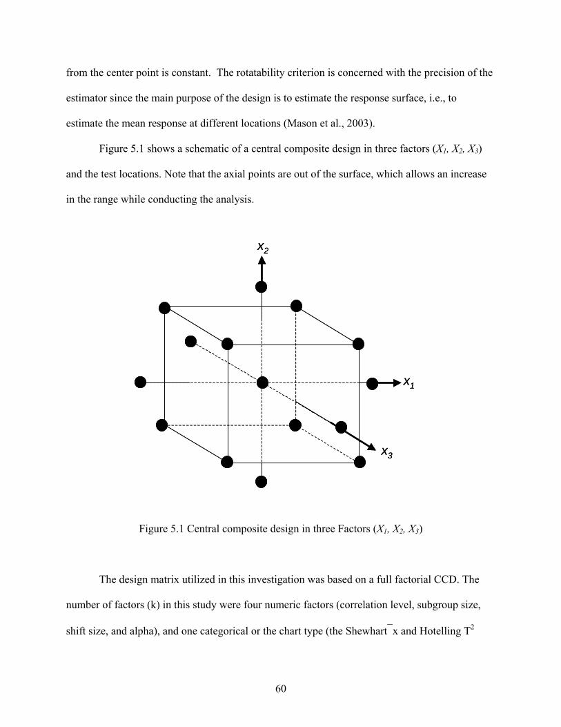
60
from the center point is constant. The rotatability criterion is concerned with the precision of the
estimator since the main purpose of the design is to estimate the response surface, i.e., to
estimate the mean response at different locations (Mason et al., 2003).
Figure 5.1 shows a schematic of a central composite design in three factors (X1, X2, X3)
and the test locations. Note that the axial points are out of the surface, which allows an increase
in the range while conducting the analysis.
Figure 5.1 Central composite design in three Factors (X1, X2, X3)
The design matrix utilized in this investigation was based on a full factorial CCD. The
number of factors (k) in this study were four numeric factors (correlation level, subgroup size,
shift size, and alpha), and one categorical or the chart type (the Shewhart⎯x and Hotelling T2
x2
x1
x3
x2
x1
x3
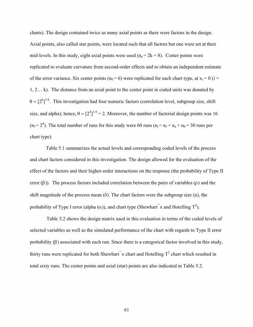
61
charts). The design contained twice as many axial points as there were factors in the design.
Axial points, also called star points, were located such that all factors but one were set at their
mid-levels. In this study, eight axial points were used (na = 2k = 8). Center points were
replicated to evaluate curvature from second-order effects and to obtain an independent estimate
of the error variance. Six center points (n0 = 6) were replicated for each chart type, at xi = 0 (i =
1, 2… k). The distance from an axial point to the center point in coded units was donated by
θ = [2k]1/4. This investigation had four numeric factors (correlation level, subgroup size, shift
size, and alpha); hence, θ = [24]1/4 = 2. Moreover, the number of factorial design points was 16
(nf = 24). The total number of runs for this study were 60 runs (nt = nf + na + n0 = 30 runs per
chart type).
Table 5.1 summarizes the actual levels and corresponding coded levels of the process
and chart factors considered in this investigation. The design allowed for the evaluation of the
effect of the factors and their higher-order interactions on the response (the probability of Type II
error (β)). The process factors included correlation between the pairs of variables (ρ) and the
shift magnitude of the process mean (δ). The chart factors were the subgroup size (n), the
probability of Type I error (alpha (α)), and chart type (Shewhart⎯x and Hotelling T2).
Table 5.2 shows the design matrix used in this evaluation in terms of the coded levels of
selected variables as well as the simulated performance of the chart with regards to Type II error
probability (β) associated with each run. Since there is a categorical factor involved in this study,
thirty runs were replicated for both Shewhart⎯x chart and Hotelling T2 chart which resulted in
total sixty runs. The center points and axial (star) points are also indicated in Table 5.2.
62
TABLE 5.1 ACTUAL VALUES AND CORRESPONDING CODED LEVELS OF THE PROCESS AND CHART VARIABLES
Variables i Factors Data Type Actual Value Coded Level
0.1 -1 0.5 0 1
Correlation (ρ) Continuous 0.9 +1 0.5 -1 1.5 0
Process
2 Shift Magnitude (δ) Continuous 2.5 +1 2.0 -1
10.0 0 3 Subgroup (n) Continuous 18.0 +1 0.001 -1 0.003 0 4 Alpha (α) Continuous 0.005 +1 ⎯x -1
Chart
5 Chart Type Categorical T2 +1
TABLE 5.2 DESIGN MATRIX
Test Point Type
Correlation (A)
Shift (B)
Subgroup Size(C)
Alpha (D)
Chart Type (E)
Response (Beta)
1 Factorial -1 -1 -1 -1 { -1 } 0.79167 2 Factorial 1 -1 -1 -1 { -1 } 0.79167 3 Factorial -1 1 -1 -1 { -1 } 0.16667 4 Factorial 1 1 -1 -1 { -1 } 0.16667 5 Factorial -1 -1 1 -1 { -1 } 0.28571 6 Factorial 1 -1 1 -1 { -1 } 0.28571 7 Factorial -1 1 1 -1 { -1 } 0.00000 8 Factorial 1 1 1 -1 { -1 } 0.00000 9 Factorial -1 -1 -1 1 { -1 } 0.66667 10 Factorial 1 -1 -1 1 { -1 } 0.66667 11 Factorial -1 1 -1 1 { -1 } 0.16667 12 Factorial 1 1 -1 1 { -1 } 0.16667 13 Factorial -1 -1 1 1 { -1 } 0.16667 14 Factorial 1 -1 1 1 { -1 } 0.16667
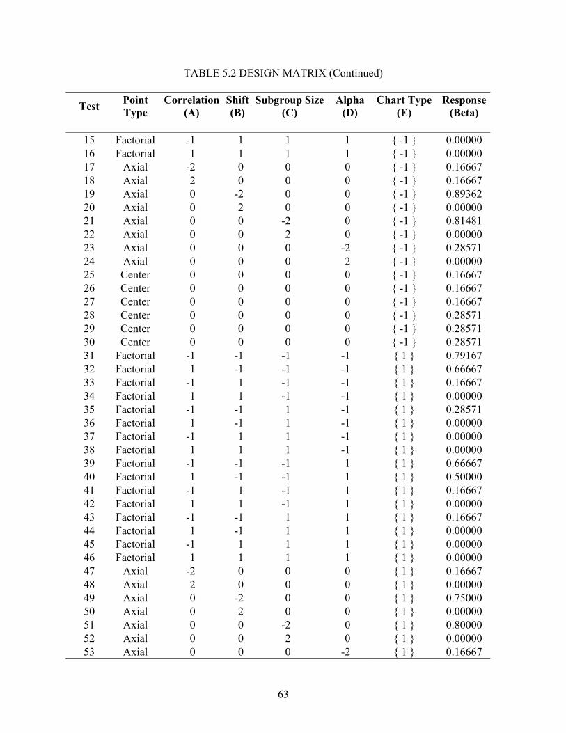
63
TABLE 5.2 DESIGN MATRIX (Continued)
Test Point Type
Correlation (A)
Shift (B)
Subgroup Size(C)
Alpha (D)
Chart Type (E)
Response (Beta)
15 Factorial -1 1 1 1 { -1 } 0.00000 16 Factorial 1 1 1 1 { -1 } 0.00000 17 Axial -2 0 0 0 { -1 } 0.16667 18 Axial 2 0 0 0 { -1 } 0.16667 19 Axial 0 -2 0 0 { -1 } 0.89362 20 Axial 0 2 0 0 { -1 } 0.00000 21 Axial 0 0 -2 0 { -1 } 0.81481 22 Axial 0 0 2 0 { -1 } 0.00000 23 Axial 0 0 0 -2 { -1 } 0.28571 24 Axial 0 0 0 2 { -1 } 0.00000 25 Center 0 0 0 0 { -1 } 0.16667 26 Center 0 0 0 0 { -1 } 0.16667 27 Center 0 0 0 0 { -1 } 0.16667 28 Center 0 0 0 0 { -1 } 0.28571 29 Center 0 0 0 0 { -1 } 0.28571 30 Center 0 0 0 0 { -1 } 0.28571 31 Factorial -1 -1 -1 -1 { 1 } 0.79167 32 Factorial 1 -1 -1 -1 { 1 } 0.66667 33 Factorial -1 1 -1 -1 { 1 } 0.16667 34 Factorial 1 1 -1 -1 { 1 } 0.00000 35 Factorial -1 -1 1 -1 { 1 } 0.28571 36 Factorial 1 -1 1 -1 { 1 } 0.00000 37 Factorial -1 1 1 -1 { 1 } 0.00000 38 Factorial 1 1 1 -1 { 1 } 0.00000 39 Factorial -1 -1 -1 1 { 1 } 0.66667 40 Factorial 1 -1 -1 1 { 1 } 0.50000 41 Factorial -1 1 -1 1 { 1 } 0.16667 42 Factorial 1 1 -1 1 { 1 } 0.00000 43 Factorial -1 -1 1 1 { 1 } 0.16667 44 Factorial 1 -1 1 1 { 1 } 0.00000 45 Factorial -1 1 1 1 { 1 } 0.00000 46 Factorial 1 1 1 1 { 1 } 0.00000 47 Axial -2 0 0 0 { 1 } 0.16667 48 Axial 2 0 0 0 { 1 } 0.00000 49 Axial 0 -2 0 0 { 1 } 0.75000 50 Axial 0 2 0 0 { 1 } 0.00000 51 Axial 0 0 -2 0 { 1 } 0.80000 52 Axial 0 0 2 0 { 1 } 0.00000 53 Axial 0 0 0 -2 { 1 } 0.16667
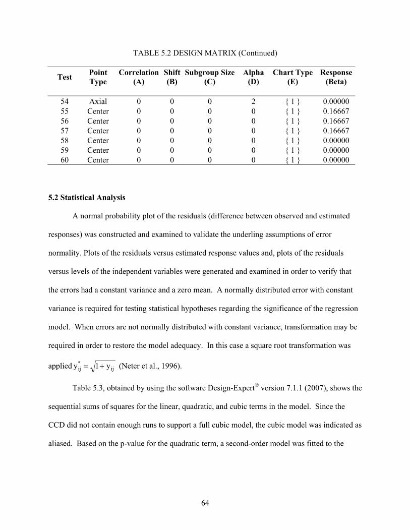
64
TABLE 5.2 DESIGN MATRIX (Continued)
Test Point Type
Correlation (A)
Shift (B)
Subgroup Size(C)
Alpha (D)
Chart Type (E)
Response (Beta)
54 Axial 0 0 0 2 { 1 } 0.00000 55 Center 0 0 0 0 { 1 } 0.16667 56 Center 0 0 0 0 { 1 } 0.16667 57 Center 0 0 0 0 { 1 } 0.16667 58 Center 0 0 0 0 { 1 } 0.00000 59 Center 0 0 0 0 { 1 } 0.00000 60 Center 0 0 0 0 { 1 } 0.00000
5.2 Statistical Analysis
A normal probability plot of the residuals (difference between observed and estimated
responses) was constructed and examined to validate the underling assumptions of error
normality. Plots of the residuals versus estimated response values and, plots of the residuals
versus levels of the independent variables were generated and examined in order to verify that
the errors had a constant variance and a zero mean. A normally distributed error with constant
variance is required for testing statistical hypotheses regarding the significance of the regression
model. When errors are not normally distributed with constant variance, transformation may be
required in order to restore the model adequacy. In this case a square root transformation was
applied ij*ij y1y += (Neter et al., 1996).
Table 5.3, obtained by using the software Design-Expert® version 7.1.1 (2007), shows the
sequential sums of squares for the linear, quadratic, and cubic terms in the model. Since the
CCD did not contain enough runs to support a full cubic model, the cubic model was indicated as
aliased. Based on the p-value for the quadratic term, a second-order model was fitted to the
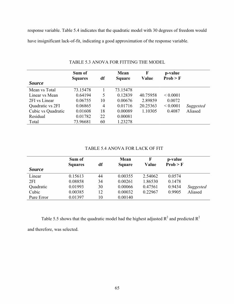
65
response variable. Table 5.4 indicates that the quadratic model with 30 degrees of freedom would
have insignificant lack-of-fit, indicating a good approximation of the response variable.
TABLE 5.3 ANOVA FOR FITTING THE MODEL
Sum of Mean F p-value
Source Squares df Square Value Prob > F
Mean vs Total 73.15478 1 73.15478 Linear vs Mean 0.64194 5 0.12839 40.75958 < 0.0001 2FI vs Linear 0.06755 10 0.00676 2.89859 0.0072 Quadratic vs 2FI 0.06865 4 0.01716 20.25363 < 0.0001 Suggested Cubic vs Quadratic 0.01608 18 0.00089 1.10305 0.4087 Aliased Residual 0.01782 22 0.00081 Total 73.96681 60 1.23278
TABLE 5.4 ANOVA FOR LACK OF FIT
Sum of Mean F p-value
Source Squares df Square Value Prob > F
Linear 0.15613 44 0.00355 2.54062 0.0574 2FI 0.08858 34 0.00261 1.86530 0.1478 Quadratic 0.01993 30 0.00066 0.47561 0.9434 Suggested Cubic 0.00385 12 0.00032 0.22967 0.9905 Aliased Pure Error 0.01397 10 0.00140
Table 5.5 shows that the quadratic model had the highest adjusted R2 and predicted R2
and therefore, was selected.
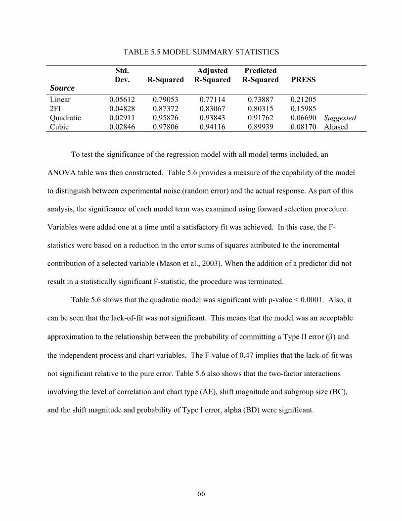
66
TABLE 5.5 MODEL SUMMARY STATISTICS
Std. Adjusted Predicted
Source Dev. R-Squared R-Squared R-Squared PRESS
Linear 0.05612 0.79053 0.77114 0.73887 0.21205 2FI 0.04828 0.87372 0.83067 0.80315 0.15985 Quadratic 0.02911 0.95826 0.93843 0.91762 0.06690 Suggested Cubic 0.02846 0.97806 0.94116 0.89939 0.08170 Aliased
To test the significance of the regression model with all model terms included, an
ANOVA table was then constructed. Table 5.6 provides a measure of the capability of the model
to distinguish between experimental noise (random error) and the actual response. As part of this
analysis, the significance of each model term was examined using forward selection procedure.
Variables were added one at a time until a satisfactory fit was achieved. In this case, the F-
statistics were based on a reduction in the error sums of squares attributed to the incremental
contribution of a selected variable (Mason et al., 2003). When the addition of a predictor did not
result in a statistically significant F-statistic, the procedure was terminated.
Table 5.6 shows that the quadratic model was significant with p-value < 0.0001. Also, it
can be seen that the lack-of-fit was not significant. This means that the model was an acceptable
approximation to the relationship between the probability of committing a Type II error (β) and
the independent process and chart variables. The F-value of 0.47 implies that the lack-of-fit was
not significant relative to the pure error. Table 5.6 also shows that the two-factor interactions
involving the level of correlation and chart type (AE), shift magnitude and subgroup size (BC),
and the shift magnitude and probability of Type I error, alpha (BD) were significant.
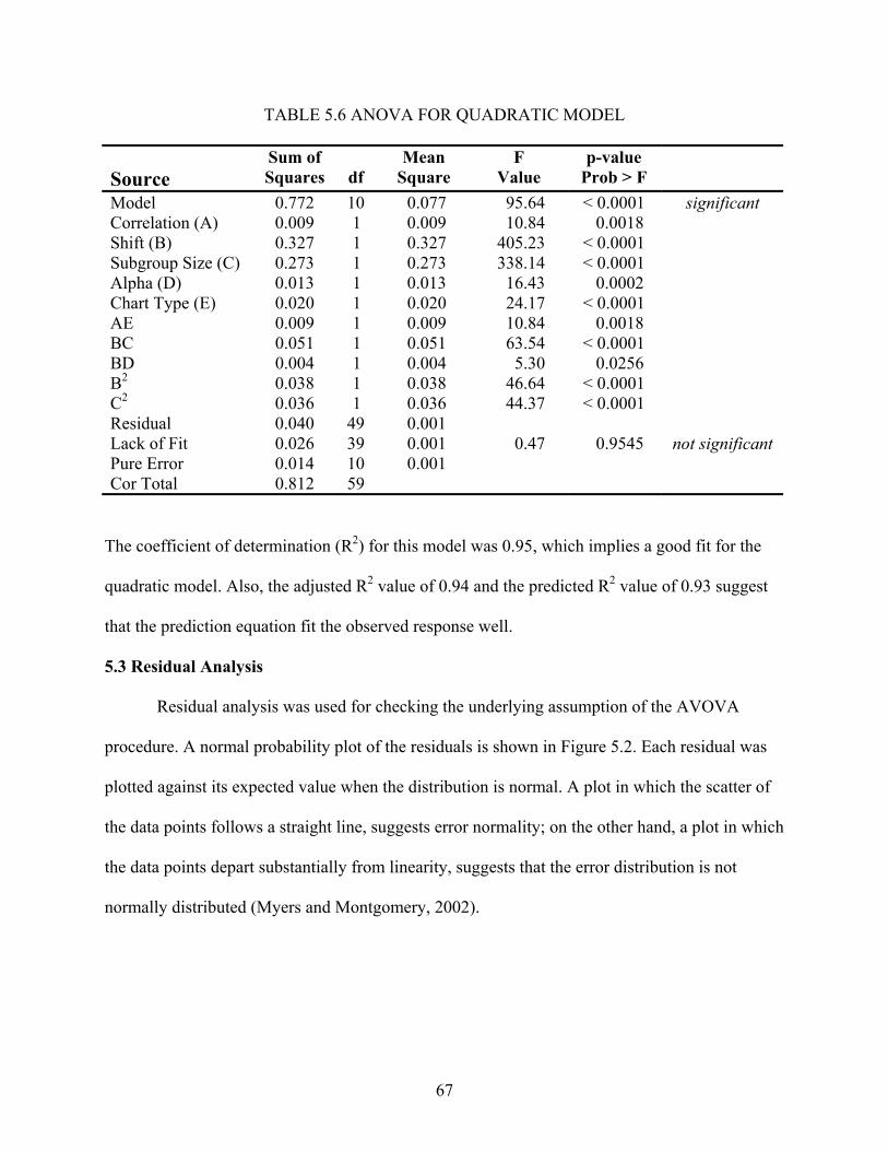
67
TABLE 5.6 ANOVA FOR QUADRATIC MODEL
Sum of Mean F p-value Source Squares df Square Value Prob > F Model 0.772 10 0.077 95.64 < 0.0001 significant Correlation (A) 0.009 1 0.009 10.84 0.0018 Shift (B) 0.327 1 0.327 405.23 < 0.0001 Subgroup Size (C) 0.273 1 0.273 338.14 < 0.0001 Alpha (D) 0.013 1 0.013 16.43 0.0002 Chart Type (E) 0.020 1 0.020 24.17 < 0.0001 AE 0.009 1 0.009 10.84 0.0018 BC 0.051 1 0.051 63.54 < 0.0001 BD 0.004 1 0.004 5.30 0.0256 B2 0.038 1 0.038 46.64 < 0.0001 C2 0.036 1 0.036 44.37 < 0.0001 Residual 0.040 49 0.001 Lack of Fit 0.026 39 0.001 0.47 0.9545 not significant Pure Error 0.014 10 0.001 Cor Total 0.812 59
The coefficient of determination (R2) for this model was 0.95, which implies a good fit for the
quadratic model. Also, the adjusted R2 value of 0.94 and the predicted R2 value of 0.93 suggest
that the prediction equation fit the observed response well.
5.3 Residual Analysis
Residual analysis was used for checking the underlying assumption of the AVOVA
procedure. A normal probability plot of the residuals is shown in Figure 5.2. Each residual was
plotted against its expected value when the distribution is normal. A plot in which the scatter of
the data points follows a straight line, suggests error normality; on the other hand, a plot in which
the data points depart substantially from linearity, suggests that the error distribution is not
normally distributed (Myers and Montgomery, 2002).
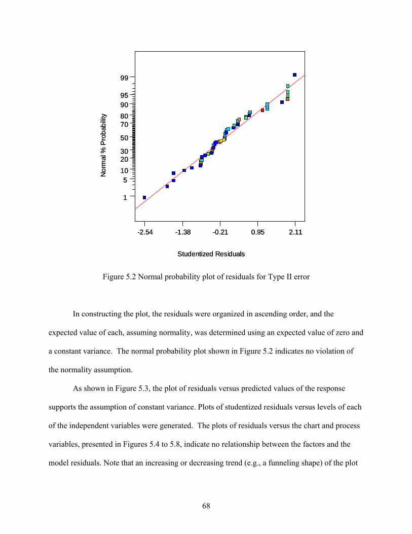
68
Figure 5.2 Normal probability plot of residuals for Type II error
In constructing the plot, the residuals were organized in ascending order, and the
expected value of each, assuming normality, was determined using an expected value of zero and
a constant variance. The normal probability plot shown in Figure 5.2 indicates no violation of
the normality assumption.
As shown in Figure 5.3, the plot of residuals versus predicted values of the response
supports the assumption of constant variance. Plots of studentized residuals versus levels of each
of the independent variables were generated. The plots of residuals versus the chart and process
variables, presented in Figures 5.4 to 5.8, indicate no relationship between the factors and the
model residuals. Note that an increasing or decreasing trend (e.g., a funneling shape) of the plot
Studentized Residuals
Nor
mal
% P
roba
bilit
y
-2.54 -1.38 -0.21 0.95 2.11
1
5102030
50
70809095
99
Studentized Residuals
Nor
mal
% P
roba
bilit
y
-2.54 -1.38 -0.21 0.95 2.11
1
5102030
50
70809095
99
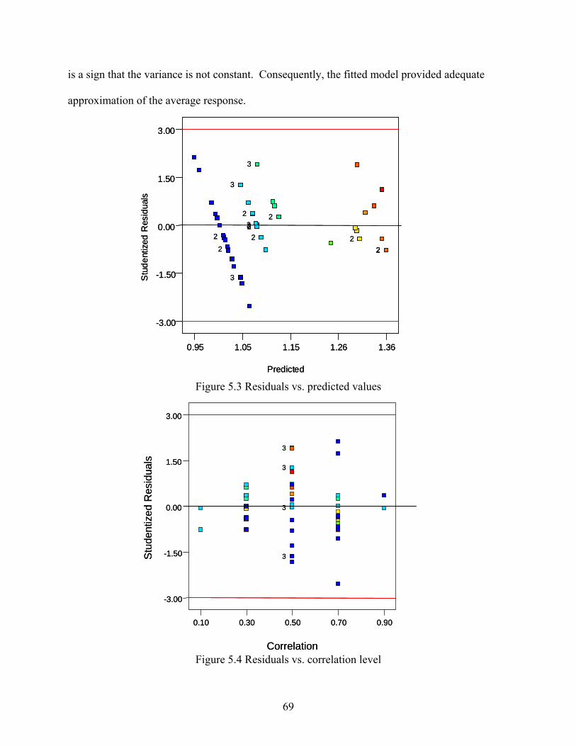
69
is a sign that the variance is not constant. Consequently, the fitted model provided adequate
approximation of the average response.
Figure 5.3 Residuals vs. predicted values
Figure 5.4 Residuals vs. correlation level
3
3
3
3
Correlation
Stu
dent
ized
Res
idua
ls
-3.00
-1.50
0.00
1.50
3.00
0.10 0.30 0.50 0.70 0.90
3
3
3
3
Correlation
Stu
dent
ized
Res
idua
ls
-3.00
-1.50
0.00
1.50
3.00
0.10 0.30 0.50 0.70 0.90
22
2
2
22
22
223
3
3
3
Predicted
Stu
dent
ized
Res
idua
ls
-3.00
-1.50
0.00
1.50
3.00
0.95 1.05 1.15 1.26 1.36
22
2
2
22
22
223
3
3
3
Predicted
Stu
dent
ized
Res
idua
ls
-3.00
-1.50
0.00
1.50
3.00
0.95 1.05 1.15 1.26 1.36
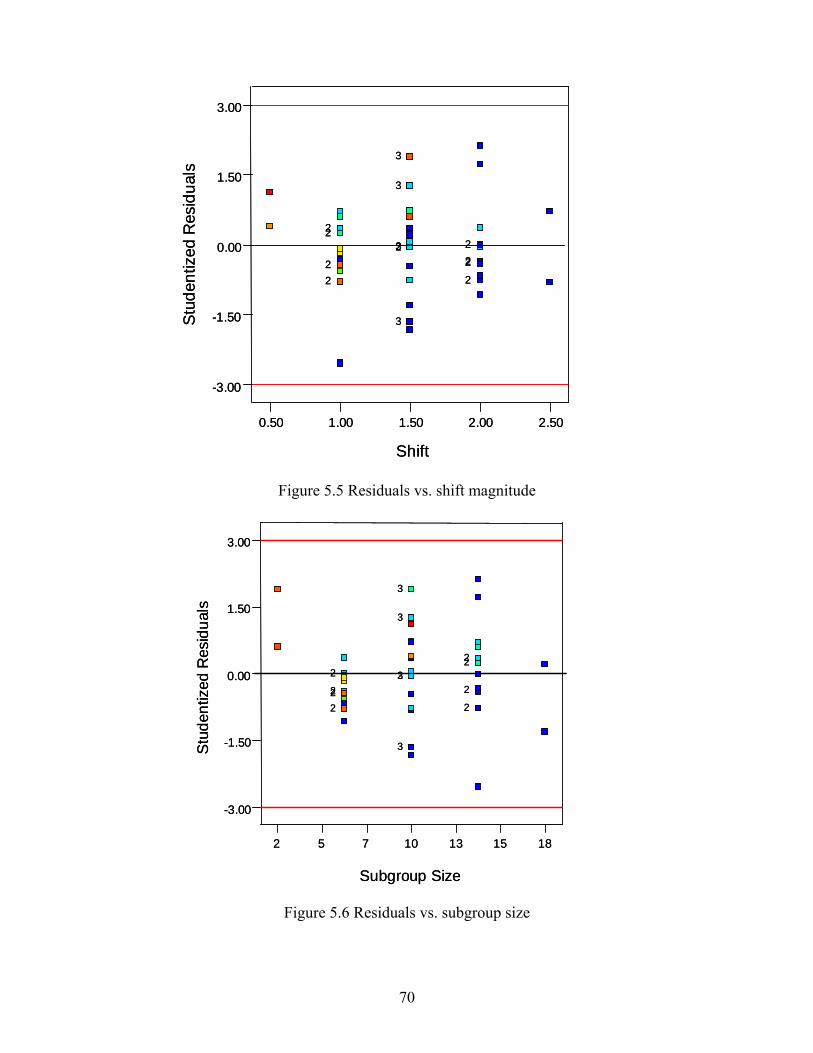
70
Figure 5.5 Residuals vs. shift magnitude
Figure 5.6 Residuals vs. subgroup size
2
2
2
22
22
223
3
3
3
Shift
Stud
entiz
edR
esid
uals
-3.00
-1.50
0.00
1.50
3.00
0.50 1.00 1.50 2.00 2.50
2
2
2
22
22
223
3
3
3
Shift
Stud
entiz
edR
esid
uals
-3.00
-1.50
0.00
1.50
3.00
0.50 1.00 1.50 2.00 2.50
2
2
2
22
22
223
3
3
3
Subgroup Size
Stu
dent
ized
Res
idua
ls
-3.00
-1.50
0.00
1.50
3.00
2 5 7 10 13 15 18
2
2
2
22
22
223
3
3
3
Subgroup Size
Stu
dent
ized
Res
idua
ls
-3.00
-1.50
0.00
1.50
3.00
2 5 7 10 13 15 18
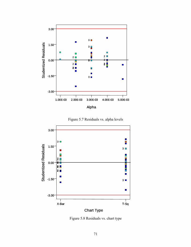
71
Figure 5.7 Residuals vs. alpha levels
Figure 5.8 Residuals vs. chart type
2
2
2
22
22
223
3
3
3
Alpha
Stu
dent
ized
Res
idua
ls
-3.00
-1.50
0.00
1.50
3.00
1.00E-03 2.00E-03 3.00E-03 4.00E-03 5.00E-03
2
2
2
22
22
223
3
3
3
Alpha
Stu
dent
ized
Res
idua
ls
-3.00
-1.50
0.00
1.50
3.00
1.00E-03 2.00E-03 3.00E-03 4.00E-03 5.00E-03
2
2
2
22
22
223
3
3
3
Chart Type
Stu
dent
ized
Res
idua
ls
-3.00
-1.50
0.00
1.50
3.00
X-Bar T-Sq
2
2
2
22
22
223
3
3
3
Chart Type
Stu
dent
ized
Res
idua
ls
-3.00
-1.50
0.00
1.50
3.00
X-Bar T-Sq
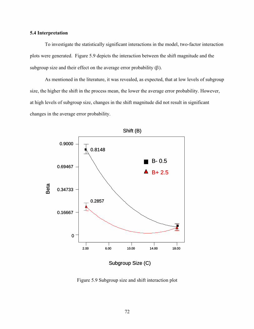
72
5.4 Interpretation
To investigate the statistically significant interactions in the model, two-factor interaction
plots were generated. Figure 5.9 depicts the interaction between the shift magnitude and the
subgroup size and their effect on the average error probability (β).
As mentioned in the literature, it was revealed, as expected, that at low levels of subgroup
size, the higher the shift in the process mean, the lower the average error probability. However,
at high levels of subgroup size, changes in the shift magnitude did not result in significant
changes in the average error probability.
Figure 5.9 Subgroup size and shift interaction plot
B- 0.5
B+ 2.5
Shift (B)
2.00 6.00 10.00 14.00 18.00
Subgroup Size (C)
0
0.34733
0.69467
0.90000.8148
0.2857
Bet
a
0.16667
B- 0.5
B+ 2.5
Shift (B)
2.00 6.00 10.00 14.00 18.00
Subgroup Size (C)
0
0.34733
0.69467
0.90000.8148
0.2857
Bet
a
0.16667
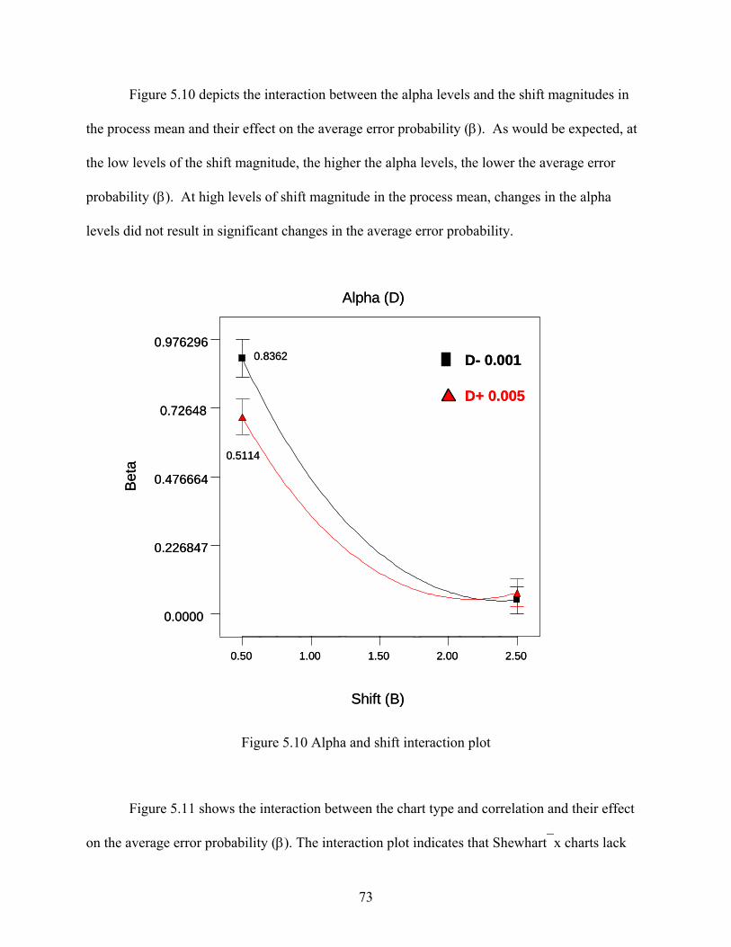
73
Figure 5.10 depicts the interaction between the alpha levels and the shift magnitudes in
the process mean and their effect on the average error probability (β). As would be expected, at
the low levels of the shift magnitude, the higher the alpha levels, the lower the average error
probability (β). At high levels of shift magnitude in the process mean, changes in the alpha
levels did not result in significant changes in the average error probability.
Figure 5.10 Alpha and shift interaction plot
Figure 5.11 shows the interaction between the chart type and correlation and their effect
on the average error probability (β). The interaction plot indicates that Shewhart⎯x charts lack
D- 0.001
D+ 0.005
Alpha (D)
0.50 1.00 1.50 2.00 2.50
Shift (B)
Beta
0.0000
0.226847
0.476664
0.72648
0.9762960.8362
0.5114
D- 0.001
D+ 0.005
Alpha (D)
0.50 1.00 1.50 2.00 2.50
Shift (B)
Beta
0.0000
0.226847
0.476664
0.72648
0.9762960.8362
0.5114
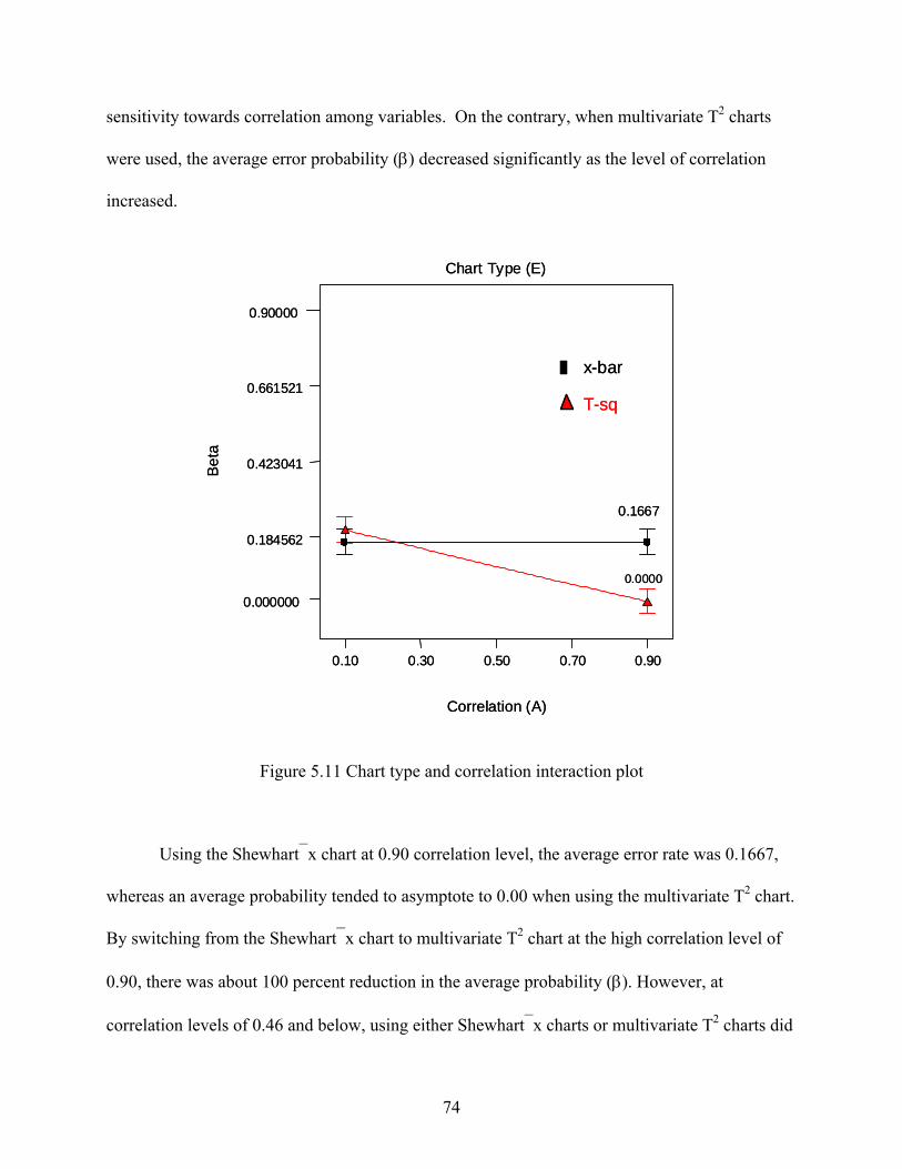
74
sensitivity towards correlation among variables. On the contrary, when multivariate T2 charts
were used, the average error probability (β) decreased significantly as the level of correlation
increased.
Figure 5.11 Chart type and correlation interaction plot
Using the Shewhart⎯x chart at 0.90 correlation level, the average error rate was 0.1667,
whereas an average probability tended to asymptote to 0.00 when using the multivariate T2 chart.
By switching from the Shewhart⎯x chart to multivariate T2 chart at the high correlation level of
0.90, there was about 100 percent reduction in the average probability (β). However, at
correlation levels of 0.46 and below, using either Shewhart⎯x charts or multivariate T2 charts did
x-bar
T-sq
Chart Type (E)
0.10 0.30 0.50 0.70 0.90
Correlation (A)
Beta
0.000000
0.184562
0.423041
0.661521
0.90000
0.0000
0.1667
x-bar
T-sq
Chart Type (E)
0.10 0.30 0.50 0.70 0.90
Correlation (A)
Beta
0.000000
0.184562
0.423041
0.661521
0.90000
0.0000
0.1667
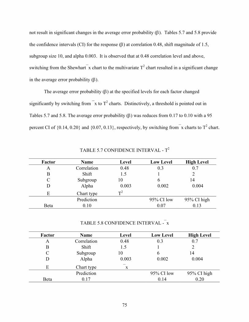
75
not result in significant changes in the average error probability (β). Tables 5.7 and 5.8 provide
the confidence intervals (CI) for the response (β) at correlation 0.48, shift magnitude of 1.5,
subgroup size 10, and alpha 0.003. It is observed that at 0.48 correlation level and above,
switching from the Shewhart⎯x chart to the multivariate T2 chart resulted in a significant change
in the average error probability (β).
The average error probability (β) at the specified levels for each factor changed
significantly by switching from ⎯x to T2 charts. Distinctively, a threshold is pointed out in
Tables 5.7 and 5.8. The average error probability (β) was reduces from 0.17 to 0.10 with a 95
percent CI of {0.14, 0.20} and {0.07, 0.13}, respectively, by switching from⎯x charts to T2 chart.
TABLE 5.7 CONFIDENCE INTERVAL - T2
Factor Name Level Low Level High Level A Correlation 0.48 0.3 0.7 B Shift 1.5 1 2 C Subgroup 10 6 14 D Alpha 0.003 0.002 0.004 E Chart type T2 Prediction 95% CI low 95% CI high
Beta 0.10 0.07 0.13
TABLE 5.8 CONFIDENCE INTERVAL -⎯x
Factor Name Level Low Level High Level A Correlation 0.48 0.3 0.7 B Shift 1.5 1 2 C Subgroup 10 6 14 D Alpha 0.003 0.002 0.004
E Chart type ⎯x Prediction 95% CI low 95% CI high
Beta 0.17 0.14 0.20
76
CHAPTER 6
ESTIMATION OF INCREMENTAL COST
In order to estimate the economic feasibility of using multivariate T2 control charts as an
alternative to the traditional univariate⎯x charts, an incremental cost model was constructed to
determine the cost or savings resulting from using multivariate T2 control charts instead of
traditional univariate⎯x charts. Only two quality characteristics were of interest. It was assumed
that the user of the⎯x charts would not have knowledge of the relationship between the two
variables and, thus, would use two separate charts to conduct the SPC tests, hence, assuming
their independence. However, the lack of the user’s knowledge of the relationship between the
two variables did not indicate that there was no correlation between them. The variables could
have had a strong dependency between them, resulting in high correlation levels (i.e. r = 0.9).
The cost model consisted of two terms. The first term was the cost of using two
separate⎯x charts to monitor the two quality characteristics of interest. The second term was the
cost of utilizing the T2 chart to monitor the two quality characteristics simultaneously. Since the
interest was to determine the cost or savings of using T2 chart as an alternative to the
traditional⎯x charts, the first term E(CU), the cost of using the⎯x chart, was multiplied by two to
include the cost associated with operating both ⎯x charts. The second term E(CM) was the cost of
using one T2 chart to monitor the same two variables. The result ΔE(C) was calculated by
subtracting the second term from the first term, which provided the cost or savings of switching
from⎯x charts to the T2 chart. Equation (6. 1) represents the cost model as
ΔE(C) = 2E(CU) – E(CM) (6.1)
77
In the univariate case, the first term E (CU) was calculated using Knappenberger and
Grandage’s (1969) economic model presented in equation (2.41). A computer program was
developed using the software MathCAD® 11 to estimate the total cost. The model was validated
and verified for five values. An illustrative example is presented in Appendix B providing all the
cost terms.
Similarly, for the multivariate case, Montgomery and Klatt’s (1972) economic model
presented in equation (2.42) was used to estimate the second term E (CM). In order to calculate
the cost of using a T2 chart, a computer subprogram was developed to calculate the probability of
Type II error (β) in the multivariate case. MathCAD®11 was utilized to develop the program,
which is presented in Figure 6.1. The sample size (N), number of variables (p), and the non-
centrality parameter (τ2) are required to calculate the probability of Type II error for the T2 chart.
To verify that the program shown in Figure 6.1 was correct, an example by Anderson
(1958) is presented in Figure 6.2. In this example, the degrees of freedom were (p = 4, and ν2 =
10). Also, the non-centrality parameter was given as (τ2 = 31.25). The null hypothesis μ0 = 0
was tested at 1 percent level of significance (α = 0.01). Figure 6.2 shows that the probability of
Type II error (β) is calculated to be 0.227. With the test of the hypothesis conducted at 5 percent
level of significance (α = 0.05), the probability of Type II error (β) droped significantly to 0.043.
Tables have been provided by Tang (1938) for the probability of Type II error (β) for
various values of (τ2) for significant levels of α = 0.01 and 0.05. These tables are provided for a
non-central parameter φ, which has a relation to τ2 as
1p +
τ=φ (6.2)
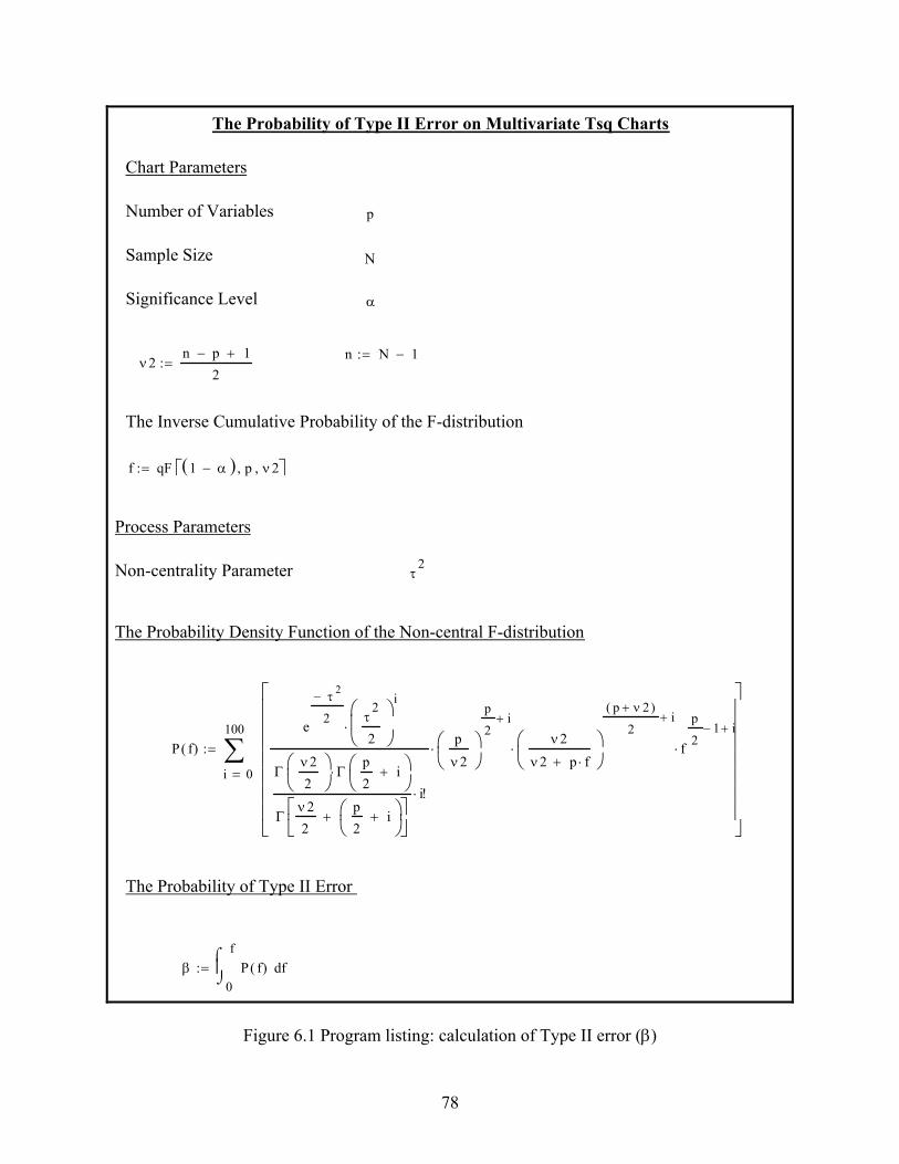
78
β0
ffP f( )
⌠⎮⌡
d:=
The Probability of Type II Error
P f( )
0
100
i
e
τ 2−
2 τ2
2
⎛⎜⎝
⎞⎟⎠
i
⋅
Γν 22
⎛⎜⎝
⎞⎟⎠
Γp2
i+⎛⎜⎝
⎞⎟⎠
⋅
Γν 22
p2
i+⎛⎜⎝
⎞⎟⎠
+⎡⎢⎣
⎤⎥⎦
i!⋅
pν 2
⎛⎜⎝
⎞⎟⎠
p
2i+
⋅ν 2
ν 2 p f⋅+⎛⎜⎝
⎞⎟⎠
p ν 2+( )
2i+
⋅ f
p
21− i+
⋅
⎡⎢⎢⎢⎢⎢⎢⎢⎣
⎤⎥⎥⎥⎥⎥⎥⎥⎦
∑=
:=
The Probability Density Function of the Non-central F-distribution
τ2Non-centrality Parameter
Process Parameters
f qF 1 α−( ) p, ν 2,⎡⎣ ⎤⎦:=
The Inverse Cumulative Probability of the F-distribution
ν 2n p− 1+
2:=
n N 1−:=
αSignificance Level
NSample Size
pNumber of Variables
Chart Parameters
The Probability of Type II Error on Multivariate Tsq Charts
Figure 6.1 Program listing: calculation of Type II error (β)
N
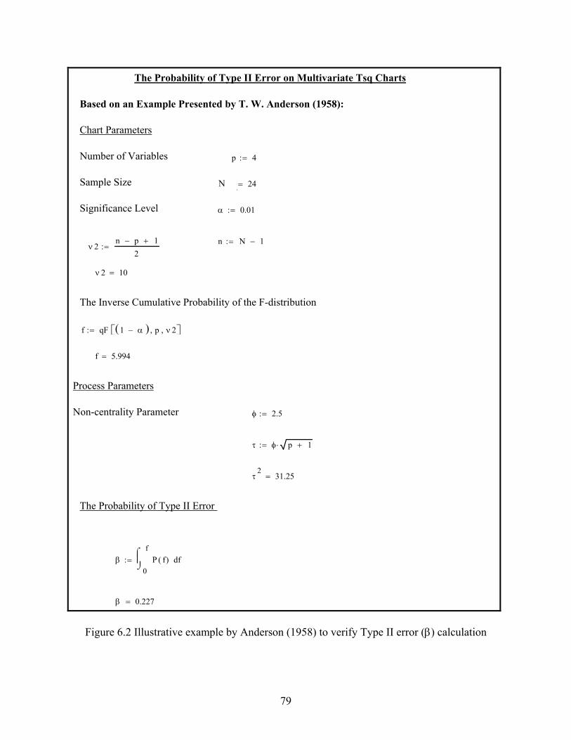
79
β 0.227=
β0
ffP f( )
⌠⎮⌡
d:=
The Probability of Type II Error
τ2
31.25=
τ φ p 1+⋅:=
φ 2.5:=Non-centrality Parameter
Process Parameters
f 5.994=
f qF 1 α−( ) p, ν 2,⎡⎣ ⎤⎦:=
The Inverse Cumulative Probability of the F-distribution
ν 2 10=
ν 2n p− 1+
2:=
n N 1−:=
α 0.01:=Significance Level
N 24:=Sample Size
p 4:=Number of Variables
Chart Parameters
Based on an Example Presented by T. W. Anderson (1958):
The Probability of Type II Error on Multivariate Tsq Charts
Figure 6.2 Illustrative example by Anderson (1958) to verify Type II error (β) calculation
N
80
Also, Tang tables are provided for p = 2, 3 …8, and ν2 = 2, 4, 6, 7… 30, and 60,
however, they do not provide the probability of Type II error (β) when ν2 = 3 and ν2 = 5. To
validate the program provided in Figure 6.1, the Tang tables were regenerated. Appendix A
provides two tables for two levels of significance (α = 0.01 and α = 0.05). Moreover, these
tables present the probability of Type II error (β) for ν2 = 3 and ν2 = 5. The program could be
used to calculate the probability of Type II error (β) under any significance levels of α.
A computer program was developed using the software MathCAD® 11 for Montgomery
and Klatt’s (1972) economic model presented in equation (2.42) to estimate the second term
E(CM). The model was validated and verified for five values. An illustrative example providing
all cost terms is presented in Appendix C.
6.1 Model Performance
To investigate the effect of the process and chart variables on the cost model, a 2k
factorial-designed experiment was performed. Since the cost estimates of this experiment were
computed analytically, a single replication of this study was required. The two levels for this
design were coded using equation (5.2). The levels were selected carefully to allow investigation
around the median values of the process and chart variables of interest. A total of six variables
were selected to investigate their effect on the response (ΔE(C)).
Four process variables and two chart variables were used in this study. The process
variables were the level of correlation (ρ) between the two variables, the shift magnitude (δ) in σ
units, the sampling frequency (K), and the cost coefficients (A1, A2, A3), where Ai = (ai.λ`)/a4,
and λ` = λ / R, R is the production rate per hour, and λ-1 is the mean time between shifts to the
out-of-control state. The parameters a1, a2, a3, and a4 are defined as follows:
a1 = fixed cost per sample
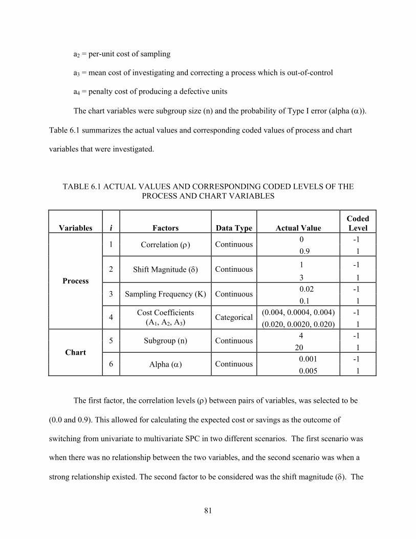
81
a2 = per-unit cost of sampling
a3 = mean cost of investigating and correcting a process which is out-of-control
a4 = penalty cost of producing a defective units
The chart variables were subgroup size (n) and the probability of Type I error (alpha (α)).
Table 6.1 summarizes the actual values and corresponding coded values of process and chart
variables that were investigated.
TABLE 6.1 ACTUAL VALUES AND CORRESPONDING CODED LEVELS OF THE PROCESS AND CHART VARIABLES
Variables i Factors Data Type Actual Value Coded Level
0 -1 1 Correlation (ρ) Continuous0.9 1
1 -1 2 Shift Magnitude (δ) Continuous3 1 0.02 -1 3 Sampling Frequency (K) Continuous0.1 1
(0.004, 0.0004, 0.004) -1
Process
4 Cost Coefficients (A1, A2, A3)
Categorical(0.020, 0.0020, 0.020) 1
4 -1 5 Subgroup (n) Continuous20 1 0.001 -1
Chart 6 Alpha (α) Continuous
0.005 1
The first factor, the correlation levels (ρ) between pairs of variables, was selected to be
(0.0 and 0.9). This allowed for calculating the expected cost or savings as the outcome of
switching from univariate to multivariate SPC in two different scenarios. The first scenario was
when there was no relationship between the two variables, and the second scenario was when a
strong relationship existed. The second factor to be considered was the shift magnitude (δ). The
82
shift magnitude levels were selected in increments of 0.5 σ at (1 and 3) to assess the effect on the
response of small and large shifts in the process mean. The third factor was the sampling
frequency (K), where levels were selected to be multiples of five at (0.02 and 0.10) to assess the
effect of sampling every (k = 20 and k = 100 units). The fourth factor was the cost coefficients
(A1, A2, A3). The cost coefficients were selected to be a categorical factor, in order to assess the
cost coefficients (A1, A2, A3) effect on the response ΔE(C) at low and high levels. The levels
were multiples of five, ranging around the median optimal cost selected by Knappenberger and
Grandage’s (1969) and Montgomery and Klatt’s (1972) economic cost models. The cost
coefficients low level was (0.004, 0.0004, and 0.004) and their high level was (0.020, 0.0020,
and 0.020). The fifth factor was the subgroup size (n), which was selected at (4 and 20) in
multiples of five to assess the effect of choosing a small as opposed to large subgroup size when
determining the expected economic cost. The sixth factor was the probability of Type I error
(alpha), which was selected in multiples of five to range around 3σ, which corresponds to
0.0027. Therefore, the alpha levels are selected at (0.001 and 0.005). In the univariate case,
alpha (α) was transformed to L = 3.29 for alpha (α) = 0.001, and to L = 2.81 for alpha (α) =
0.005.
In conducting this study, the assumptions made by Knappenberger and Grandage’s
(1969) model were used for calculating both terms of the incremental cost model. The first
assumption was that, on the average, the process shifts out-of-control after every 1,000 units (λ`
= 0.001). The second assumption was that, the penalty cost of producing a defective product (a4
= $10). For this investigation, a 26 factorial design was employed. The total number of tests was
64. Table 6.2 provides the design matrix used in this evaluation in terms of the coded levels of
the process and chart variables, as well as the ΔE(C) associated with each cost estimate.
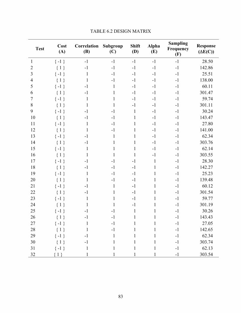
83
TABLE 6.2 DESIGN MATRIX
Test Cost (A)
Correlation (B)
Subgroup (C)
Shift (D)
Alpha (E)
Sampling Frequency
(F)
Response (ΔE(C))
1 { -1 } -1 -1 -1 -1 -1 28.50 2 { 1 } -1 -1 -1 -1 -1 142.86 3 { -1 } 1 -1 -1 -1 -1 25.51 4 { 1 } 1 -1 -1 -1 -1 138.00 5 { -1 } -1 1 -1 -1 -1 60.11 6 { 1 } -1 1 -1 -1 -1 301.47 7 { -1 } 1 1 -1 -1 -1 59.74 8 { 1 } 1 1 -1 -1 -1 301.11 9 { -1 } -1 -1 1 -1 -1 30.24 10 { 1 } -1 -1 1 -1 -1 143.47 11 { -1 } 1 -1 1 -1 -1 27.80 12 { 1 } 1 -1 1 -1 -1 141.00 13 { -1 } -1 1 1 -1 -1 62.34 14 { 1 } -1 1 1 -1 -1 303.76 15 { -1 } 1 1 1 -1 -1 62.14 16 { 1 } 1 1 1 -1 -1 303.55 17 { -1 } -1 -1 -1 1 -1 28.30 18 { 1 } -1 -1 -1 1 -1 142.27 19 { -1 } 1 -1 -1 1 -1 25.23 20 { 1 } 1 -1 -1 1 -1 139.48 21 { -1 } -1 1 -1 1 -1 60.12 22 { 1 } -1 1 -1 1 -1 301.54 23 { -1 } 1 1 -1 1 -1 59.77 24 { 1 } 1 1 -1 1 -1 301.19 25 { -1 } -1 -1 1 1 -1 30.26 26 { 1 } -1 -1 1 1 -1 143.43 27 { -1 } 1 -1 1 1 -1 27.05 28 { 1 } 1 -1 1 1 -1 142.65 29 { -1 } -1 1 1 1 -1 62.34 30 { 1 } -1 1 1 1 -1 303.74 31 { -1 } 1 1 1 1 -1 62.13 32 { 1 } 1 1 1 1 -1 303.54
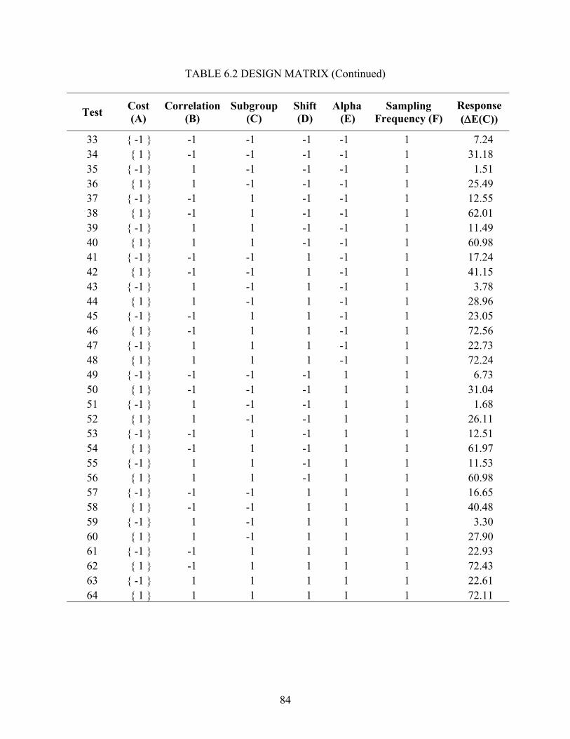
84
TABLE 6.2 DESIGN MATRIX (Continued)
Test Cost (A)
Correlation (B)
Subgroup (C)
Shift (D)
Alpha (E)
Sampling Frequency (F)
Response (ΔE(C))
33 { -1 } -1 -1 -1 -1 1 7.24 34 { 1 } -1 -1 -1 -1 1 31.18 35 { -1 } 1 -1 -1 -1 1 1.51 36 { 1 } 1 -1 -1 -1 1 25.49 37 { -1 } -1 1 -1 -1 1 12.55 38 { 1 } -1 1 -1 -1 1 62.01 39 { -1 } 1 1 -1 -1 1 11.49 40 { 1 } 1 1 -1 -1 1 60.98 41 { -1 } -1 -1 1 -1 1 17.24 42 { 1 } -1 -1 1 -1 1 41.15 43 { -1 } 1 -1 1 -1 1 3.78 44 { 1 } 1 -1 1 -1 1 28.96 45 { -1 } -1 1 1 -1 1 23.05 46 { 1 } -1 1 1 -1 1 72.56 47 { -1 } 1 1 1 -1 1 22.73 48 { 1 } 1 1 1 -1 1 72.24 49 { -1 } -1 -1 -1 1 1 6.73 50 { 1 } -1 -1 -1 1 1 31.04 51 { -1 } 1 -1 -1 1 1 1.68 52 { 1 } 1 -1 -1 1 1 26.11 53 { -1 } -1 1 -1 1 1 12.51 54 { 1 } -1 1 -1 1 1 61.97 55 { -1 } 1 1 -1 1 1 11.53 56 { 1 } 1 1 -1 1 1 60.98 57 { -1 } -1 -1 1 1 1 16.65 58 { 1 } -1 -1 1 1 1 40.48 59 { -1 } 1 -1 1 1 1 3.30 60 { 1 } 1 -1 1 1 1 27.90 61 { -1 } -1 1 1 1 1 22.93 62 { 1 } -1 1 1 1 1 72.43 63 { -1 } 1 1 1 1 1 22.61 64 { 1 } 1 1 1 1 1 72.11
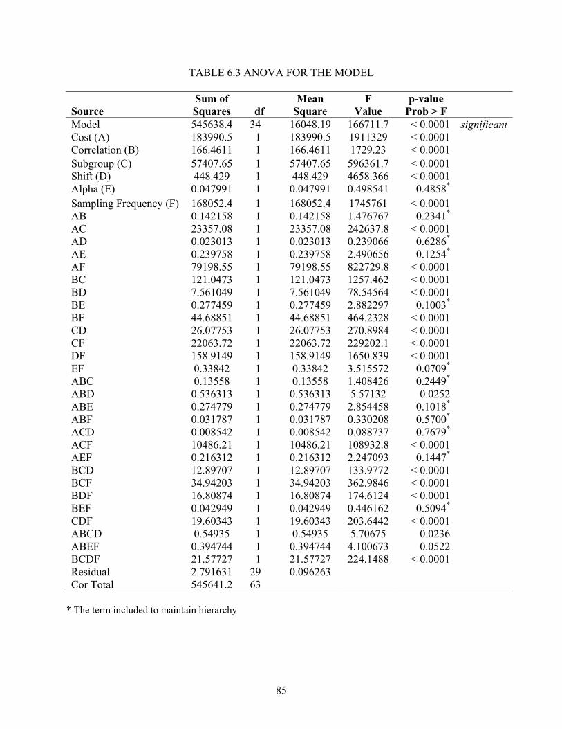
85
TABLE 6.3 ANOVA FOR THE MODEL
Sum of Mean F p-value Source Squares df Square Value Prob > F Model 545638.4 34 16048.19 166711.7 < 0.0001 significantCost (A) 183990.5 1 183990.5 1911329 < 0.0001 Correlation (B) 166.4611 1 166.4611 1729.23 < 0.0001 Subgroup (C) 57407.65 1 57407.65 596361.7 < 0.0001 Shift (D) 448.429 1 448.429 4658.366 < 0.0001 Alpha (E) 0.047991 1 0.047991 0.498541 0.4858* Sampling Frequency (F) 168052.4 1 168052.4 1745761 < 0.0001 AB 0.142158 1 0.142158 1.476767 0.2341* AC 23357.08 1 23357.08 242637.8 < 0.0001 AD 0.023013 1 0.023013 0.239066 0.6286* AE 0.239758 1 0.239758 2.490656 0.1254* AF 79198.55 1 79198.55 822729.8 < 0.0001 BC 121.0473 1 121.0473 1257.462 < 0.0001 BD 7.561049 1 7.561049 78.54564 < 0.0001 BE 0.277459 1 0.277459 2.882297 0.1003* BF 44.68851 1 44.68851 464.2328 < 0.0001 CD 26.07753 1 26.07753 270.8984 < 0.0001 CF 22063.72 1 22063.72 229202.1 < 0.0001 DF 158.9149 1 158.9149 1650.839 < 0.0001 EF 0.33842 1 0.33842 3.515572 0.0709* ABC 0.13558 1 0.13558 1.408426 0.2449* ABD 0.536313 1 0.536313 5.57132 0.0252 ABE 0.274779 1 0.274779 2.854458 0.1018* ABF 0.031787 1 0.031787 0.330208 0.5700* ACD 0.008542 1 0.008542 0.088737 0.7679* ACF 10486.21 1 10486.21 108932.8 < 0.0001 AEF 0.216312 1 0.216312 2.247093 0.1447* BCD 12.89707 1 12.89707 133.9772 < 0.0001 BCF 34.94203 1 34.94203 362.9846 < 0.0001 BDF 16.80874 1 16.80874 174.6124 < 0.0001 BEF 0.042949 1 0.042949 0.446162 0.5094* CDF 19.60343 1 19.60343 203.6442 < 0.0001 ABCD 0.54935 1 0.54935 5.70675 0.0236 ABEF 0.394744 1 0.394744 4.100673 0.0522 BCDF 21.57727 1 21.57727 224.1488 < 0.0001 Residual 2.791631 29 0.096263 Cor Total 545641.2 63
* The term included to maintain hierarchy
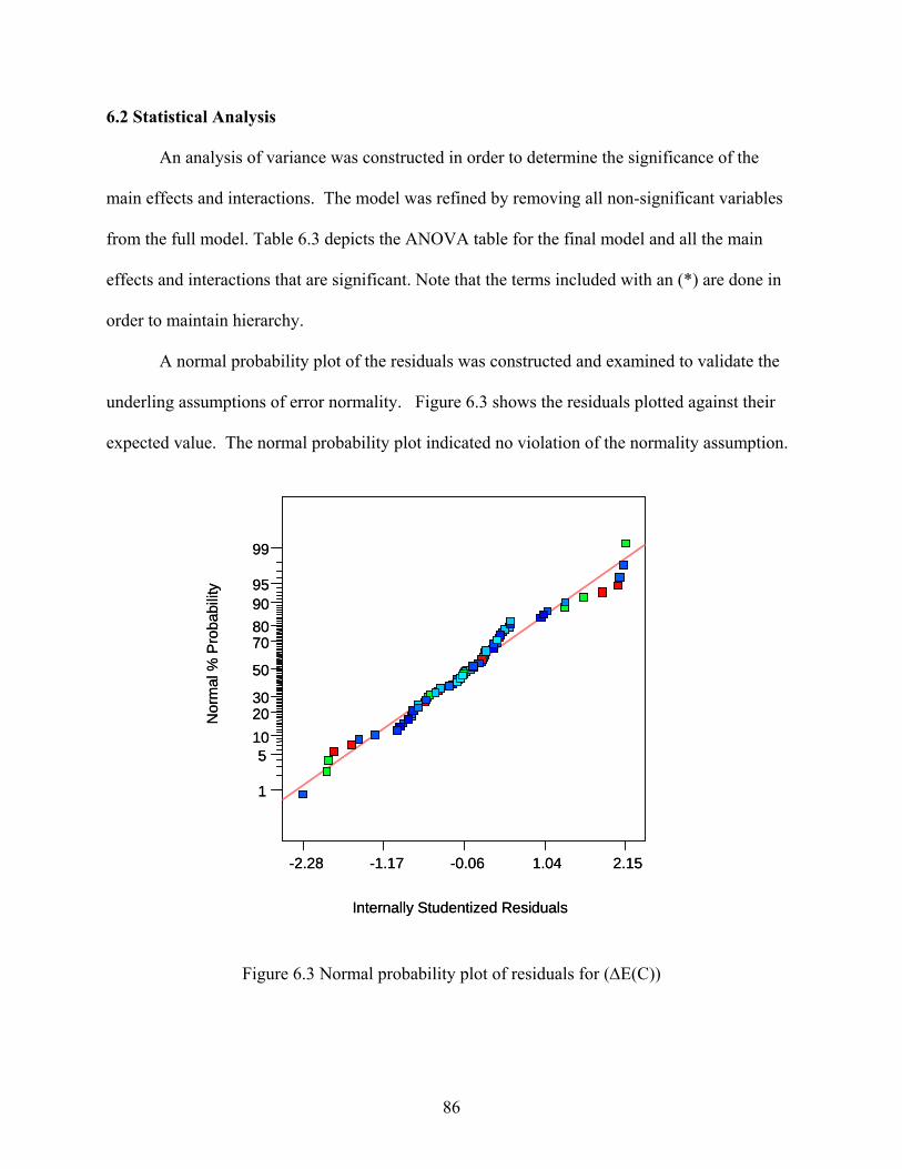
86
6.2 Statistical Analysis
An analysis of variance was constructed in order to determine the significance of the
main effects and interactions. The model was refined by removing all non-significant variables
from the full model. Table 6.3 depicts the ANOVA table for the final model and all the main
effects and interactions that are significant. Note that the terms included with an (*) are done in
order to maintain hierarchy.
A normal probability plot of the residuals was constructed and examined to validate the
underling assumptions of error normality. Figure 6.3 shows the residuals plotted against their
expected value. The normal probability plot indicated no violation of the normality assumption.
Figure 6.3 Normal probability plot of residuals for (ΔE(C))
Internally Studentized Residuals
Nor
mal
% P
roba
bilit
y
-2.28 -1.17 -0.06 1.04 2.15
1
5102030
50
70809095
99
Internally Studentized Residuals
Nor
mal
% P
roba
bilit
y
-2.28 -1.17 -0.06 1.04 2.15
1
5102030
50
70809095
99
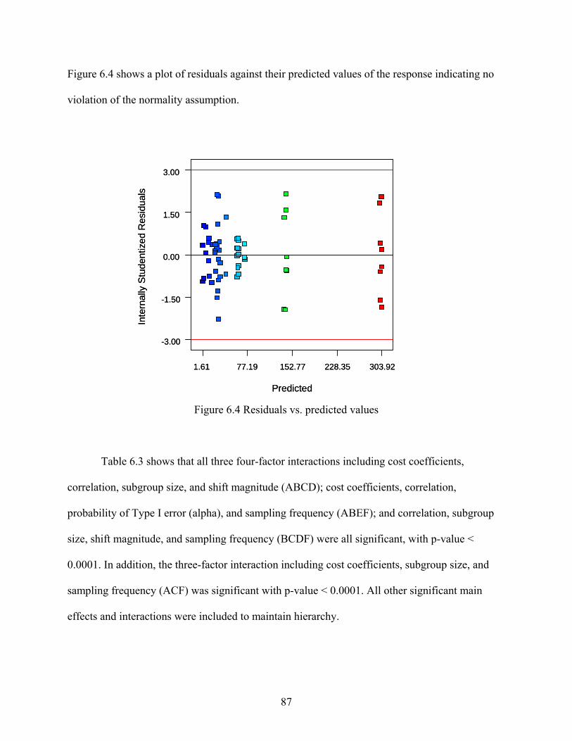
87
Figure 6.4 shows a plot of residuals against their predicted values of the response indicating no
violation of the normality assumption.
Figure 6.4 Residuals vs. predicted values
Table 6.3 shows that all three four-factor interactions including cost coefficients,
correlation, subgroup size, and shift magnitude (ABCD); cost coefficients, correlation,
probability of Type I error (alpha), and sampling frequency (ABEF); and correlation, subgroup
size, shift magnitude, and sampling frequency (BCDF) were all significant, with p-value <
0.0001. In addition, the three-factor interaction including cost coefficients, subgroup size, and
sampling frequency (ACF) was significant with p-value < 0.0001. All other significant main
effects and interactions were included to maintain hierarchy.
Predicted
Inte
rnal
ly S
tude
ntiz
edR
esid
uals
-3.00
-1.50
0.00
1.50
3.00
1.61 77.19 152.77 228.35 303.92
Predicted
Inte
rnal
ly S
tude
ntiz
edR
esid
uals
-3.00
-1.50
0.00
1.50
3.00
1.61 77.19 152.77 228.35 303.92
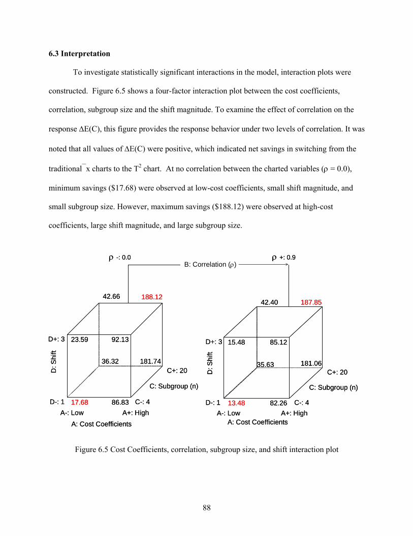
88
6.3 Interpretation
To investigate statistically significant interactions in the model, interaction plots were
constructed. Figure 6.5 shows a four-factor interaction plot between the cost coefficients,
correlation, subgroup size and the shift magnitude. To examine the effect of correlation on the
response ΔE(C), this figure provides the response behavior under two levels of correlation. It was
noted that all values of ΔE(C) were positive, which indicated net savings in switching from the
traditional⎯x charts to the T2 chart. At no correlation between the charted variables (ρ = 0.0),
minimum savings ($17.68) were observed at low-cost coefficients, small shift magnitude, and
small subgroup size. However, maximum savings ($188.12) were observed at high-cost
coefficients, large shift magnitude, and large subgroup size.
Figure 6.5 Cost Coefficients, correlation, subgroup size, and shift interaction plot
A: Cost Coefficients
D: S
hift
C: Subgroup (n)
A-: Low A+: HighD-: 1
D+: 3
C-: 4
C+: 20
13.48
35.63
15.48
42.40
82.26
181.06
85.12
187.85
ρ -: 0.0
A: Cost Coefficients
D: S
hift
C: Subgroup (n)
A-: Low A+: HighD-: 1
D+: 3
C-: 4
C+: 20
17.68
36.32
23.59
42.66
86.83
181.74
92.13
188.12
ρ +: 0.9B: Correlation (ρ)
A: Cost Coefficients
D: S
hift
C: Subgroup (n)
A-: Low A+: HighD-: 1
D+: 3
C-: 4
C+: 20
13.48
35.63
15.48
42.40
82.26
181.06
85.12
187.85
ρ -: 0.0
A: Cost Coefficients
D: S
hift
C: Subgroup (n)
A-: Low A+: HighD-: 1
D+: 3
C-: 4
C+: 20
17.68
36.32
23.59
42.66
86.83
181.74
92.13
188.12
ρ +: 0.9B: Correlation (ρ)
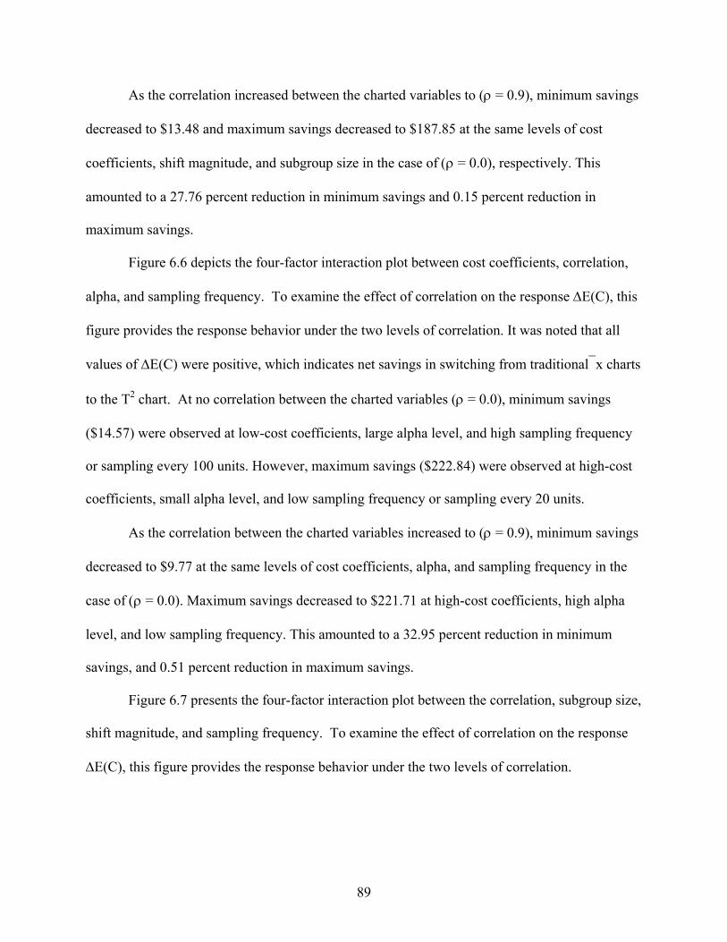
89
As the correlation increased between the charted variables to (ρ = 0.9), minimum savings
decreased to $13.48 and maximum savings decreased to $187.85 at the same levels of cost
coefficients, shift magnitude, and subgroup size in the case of (ρ = 0.0), respectively. This
amounted to a 27.76 percent reduction in minimum savings and 0.15 percent reduction in
maximum savings.
Figure 6.6 depicts the four-factor interaction plot between cost coefficients, correlation,
alpha, and sampling frequency. To examine the effect of correlation on the response ΔE(C), this
figure provides the response behavior under the two levels of correlation. It was noted that all
values of ΔE(C) were positive, which indicates net savings in switching from traditional⎯x charts
to the T2 chart. At no correlation between the charted variables (ρ = 0.0), minimum savings
($14.57) were observed at low-cost coefficients, large alpha level, and high sampling frequency
or sampling every 100 units. However, maximum savings ($222.84) were observed at high-cost
coefficients, small alpha level, and low sampling frequency or sampling every 20 units.
As the correlation between the charted variables increased to (ρ = 0.9), minimum savings
decreased to $9.77 at the same levels of cost coefficients, alpha, and sampling frequency in the
case of (ρ = 0.0). Maximum savings decreased to $221.71 at high-cost coefficients, high alpha
level, and low sampling frequency. This amounted to a 32.95 percent reduction in minimum
savings, and 0.51 percent reduction in maximum savings.
Figure 6.7 presents the four-factor interaction plot between the correlation, subgroup size,
shift magnitude, and sampling frequency. To examine the effect of correlation on the response
ΔE(C), this figure provides the response behavior under the two levels of correlation.
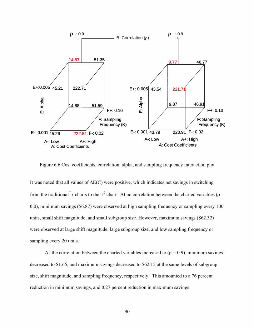
90
Figure 6.6 Cost coefficients, correlation, alpha, and sampling frequency interaction plot
It was noted that all values of ΔE(C) were positive, which indicates net savings in switching
from the traditional⎯x charts to the T2 chart. At no correlation between the charted variables (ρ =
0.0), minimum savings ($6.87) were observed at high sampling frequency or sampling every 100
units, small shift magnitude, and small subgroup size. However, maximum savings ($62.32)
were observed at large shift magnitude, large subgroup size, and low sampling frequency or
sampling every 20 units.
As the correlation between the charted variables increased to (ρ = 0.9), minimum savings
decreased to $1.65, and maximum savings decreased to $62.15 at the same levels of subgroup
size, shift magnitude, and sampling frequency, respectively. This amounted to a 76 percent
reduction in minimum savings, and 0.27 percent reduction in maximum savings.
A: Cost CoefficientsE
: Alp
haA-: Low A+: High
E-: 0.001
E+: 0.005
F-: 0.02
F+: 0.10
43.79
9.87
43.54
9.77
220.91
46.91
221.71
46.77
A: Cost Coefficients
E: A
lpha
F: SamplingFrequency (K)
A-: Low A+: High
E-: 0.001
E+:0.005
F-: 0.02
F+: 0.10
45.26
14.88
45.21
14.57
222.84
51.59
222.71
51.35
ρ -: 0.0 ρ +: 0.9B: Correlation (ρ)
F: SamplingFrequency (K)

91
Figure 6.7 Correlation, subgroup size, shift magnitude, and sampling frequency interaction plot
Figure 6.8 shows the three-factor interaction plot between the cost coefficients, subgroup size,
and sampling frequency.
Minimum savings ($11.95) occurred at low-cost coefficients, high sampling frequency or
sampling every 100 units, and small subgroup size. However, maximum savings ($302.65) were
observed at high-cost coefficients, large subgroup size, and low sampling frequency or sampling
every 20 units. From figure 6.8, it is noted that all values of ΔE(C) are positive, which indicates
net savings in switching from the traditional⎯x charts to the T2 chart.
C: S
ubgr
oup
(n)
D: Shift
F-: 0.02 F+: 0.10
C-: 4
C+: 20
D-: 1
D+: 3
25.30
27.45
59.78
62.15
1.65
3.51
11.48
22.64
F: Sampling Frequency (K)
C: S
ubgr
oup
(n)
D: Shift
F-: 0.02 F+: 0.10
C-: 4
C+: 20
D-: 1
D+: 3
28.50
30.18
60.09
62.32
6.87
17.01
12.54
23.01
ρ -: 0.0 ρ +: 0.9B: Correlation (ρ)
F: Sampling Frequency (K)
C: S
ubgr
oup
(n)
D: Shift
F-: 0.02 F+: 0.10
C-: 4
C+: 20
D-: 1
D+: 3
25.30
27.45
59.78
62.15
1.65
3.51
11.48
22.64
F: Sampling Frequency (K)
C: S
ubgr
oup
(n)
D: Shift
F-: 0.02 F+: 0.10
C-: 4
C+: 20
D-: 1
D+: 3
28.50
30.18
60.09
62.32
6.87
17.01
12.54
23.01
ρ -: 0.0 ρ +: 0.9B: Correlation (ρ)
F: Sampling Frequency (K)

92
Figure 6.8 Cost coefficients, subgroup size, and sampling frequency interaction plot
Results of this study are based on the assumptions made for rate of production, penalty of
producing a defective unit, and levels of process and chart variables specified in this
investigation.
A: Cost
C: S
ubgr
oup
(n)
F: K
A-: Low A+: High
C-: 4
C+: 20
F-: 0.02
F+: 0.10
29.34
11.95
61.21
17.78
142.98
35.98
302.65
67.22
A: Cost
C: S
ubgr
oup
(n)
F: K
A-: Low A+: High
C-: 4
C+: 20
F-: 0.02
F+: 0.10
29.34
11.95
61.21
17.78
142.98
35.98
302.65
67.22
93
CHAPTER 7
SUMMARY AND CONCLUSIONS
This research offered a comprehensive review of the literature pertaining to multivariate
control charts and their underlying assumptions. It also reviewed the literature concerning the
economic design of control charts for both univariate and multivariate applications. Levels of
correlation that mandate the use of multivariate charts and the statistical effect of mis-specifying
the process model while applying traditional Shewhart charts was not provided in the literature.
In addition, estimates of the economic feasibility of using multivariate T2 control charts as an
alternative to traditional univariate⎯x charts was not supplied.
Advancements in technology have raised the need for simultaneous monitoring of several
quality characteristics that could be correlated. This need is served best by utilizing multivariate
SPC techniques. However, multivariate control charting procedures are computationally
intensive, which make multivariate SPC less popular. Increased availability of high-speed
computers and statistical software programs, formerly available only to very few, has made the
statistical computations of multivariate SPC easier. The lack of knowledge of the correlation
between quality characteristics being charted does not mean that the relationship is absent.
7.1 Summary and Results
The objective of this research was twofold. The first objective was to identify levels of
correlation between quality characteristics at which the statistical performance of multiple⎯x
control charts deteriorate in comparison to an equivalent T2 chart. In achieving this objective,
simulated data was analyzed using⎯x and T2 charts for the case of two quality characteristics.
Chapters 4 and 5 present the simulation analyses and results. A central composite design was
chosen to examine the effect of changes in the level of correlation between characteristics
94
coupled with changes in the process model and chart design variables. The process variables
included correlation between the pairs of characteristics (ρ) and the shift magnitude of the
process mean (δ). The chart variables were comprised of the subgroup size (n) and the
probability of Type I error (α). This study was conducted for the two chart types (Shewhart⎯x
and Hotelling T2). It was concluded that when using the T2 chart, changes in the level of
correlation between the characteristics did not result in a significant increase in the average
probability error (α). On the contrary, while using the⎯x chart, changes in the level of
correlation resulted in a significant difference in the average probability of Type I error. As the
correlation level increased to 0.8 a 32 percent increase in the average rate of false alarms (α)
occurred. In addition, a threshold was identified at (ρ ≥ 0.48), indicating deterioration in the
performance of the⎯x charts in comparison to the T2 chart. Due to the quadratic effect of the
correlation coefficient ρ, it could be concluded that a similar threshold exists at (ρ ≤ - 0.48).
Using the T2 chart as an alternative SPC technique to the⎯x chart resulted in a significant
reduction in the average probability of Type II error (β).
The second objective was to assess the economic feasibility of utilizing the T2 chart as an
alternative to the⎯x chart. This investigation was conducted for the case of two quality
characteristics, by utilizing the economic design models developed by Knappenberger and
Grandage’s (1969), and Montgomery and Klatt’s (1972). An incremental cost model was
constructed to examine the cost and worth of switching from univariate to multivariate SPC
techniques under specified levels of process and chart variables. Chapter 6 provides the
economic benefits of using a T2 chart instead of two⎯x charts. A computer program was created
using MathCAD® 11 software for this application. A 26 factorial-design was performed. Four
95
process variables and two chart variables were considered. The level of correlation (ρ) between
the two characteristics varied from 0.0 to 0.9. The process variables included the shift
magnitude, sampling frequency, and the cost coefficients. The chart variables included the
subgroup size and the probability of Type I error. The results indicated that using a T2 chart for
monitoring two characteristics whether they are correlated or not, will result in significant net
savings. However, when the characteristics are highly correlated, the net savings were reduced
due to the increased power of the T2 chart.
7.2 Future Research
Future research in this area could be extended to include the statistical performance of
the⎯x chart in comparison to the T2 chart for more than two variables under different levels of
correlation. Moreover, future research on the statistical performance of control charts could
include more sensitive charting techniques such as the CUSUM and EWMA and their
multivariate direct analog charts.
The incremental cost model constructed in this research could also be extended to
examine the cost and worth of switching from univariate to multivariate SPC techniques in the
case of more than two quality characteristics. In addition, the economic cost models that were
employed are traditional economic models that are mainly utilized to maintain current quality
levels. Further investigation could be conducted employing proactive economic models that are
designed to achieve improved levels of performance.

96
REFERENCES
97
LIST OF REFERENCES
Alexander, S.M., Dillman, M.A., Usher, J.S., and Damodaran, B., 1995, “Economic Design of Control Charts Using the Taguchi Loss Function”, Computers and Industrial Engineering, Vol. 28, No. 3, pp. 671-679. Alt, F.B., 1973, “Aspects of Multivariate Control Charts”. M.S. thesis, Georgia Institute of Technology, Atlanta. Alt, F.B., 1982, “Multivariate Quality Control: State of the Art”, Transactions of the 1982 ASQC Quality Congress, Detroit, MI, pp. 886-893. Alt, F.B., (1984), “Multivariate Quality Control”, The Encyclopedia of Statistical Sciences, edited by N.L. Johnson and S. Kots, Wiley, New York, pp. 110-122. Alt, F.B., Goode, J.J., and Wadsworth, H.M., 1976, “Small Sample Limits for the Mean of a Multivariate Normal Process” ASQC Annual Technology Conference Transactions, Toronto, pp. 170 – 176. Alt, F.B., and Smith, N.D., 1988, “Multivariate Process Control”, in Handbook of Statistics, edited by P.R. Krishnaiah and C.R. Rao, North-Holland, Amsterdam, Vol. 7, pp. 333-352. Anderson, T.W., 1958, An Introduction to Multivariate Statistical Analysis, Second Edition, John Wiley and Sons, Inc., New York. Boyles, R.A., 1996, “Exploratory Capability Analysis”, Journal of Quality Technology, Vol. 28, pp. 91-98. Crosier, R.B., 1988, “Multivariate Generalizations of Cumulative Sum Quality Control Schemes”, Technometrics, Vol. 30, pp. 291-303. Del Castillo, E., 2002, Statistical Process Adjustment for Quality Control, John Wiley and Sons, Inc., New York. Duncan, A.J., 1956, “The Economic Design of⎯x Charts Used to Maintain Current Control of the Process”, Journal of American Statistical Association, Vol. 51, pp. 228– 242. Ghare, P.M., and Torgersen, P.E., 1968, “The Multi-Characteristics Control Chart”, Journal of Industrial Engineering, Vol. 19, pp. 269– 272. Hawkins, D.M., 1991, “Multivariate Quality Control Based on Regression- Adjusted Variables”, Technometrics, Vol. 33, pp. 61-75. Healy, J.D., 1987, “A Note on Multivariate CUSUM Procedures”, Technometrics, Vol. 29, pp. 409 – 412.
98
Hotelling, H.H., 1931, “The Generalization of Student’s Ratio”, Annals of Mathematical Statistics, Vol. 2, pp. 360 – 378. Hotelling, H.H., 1947, “Multivariate Quality Control - Illustrated by the Air Testing of Sample Bombsights”, in Techniques of Statistical Analysis, Eisenhart C., Hastay M.W., and Wallis W.A., (eds) McGraw-Hill, New York, pp. 111-184. Hubele, N.F., Shahriari, H., and Cheng, C.S., 1991, “A Bivariate Process Capability Vector, in Statistics and Design in Process Control”, in Statistical Process Control in Manufacturing edited by Keats, J.B., and Montgomery, D.C., Marcel Dekker, New York, NY. pp. 299-310. Jackson, J.E., 1956, “Quality Control Methods for Two Related Variables”, Industrial Quality Control, Vol. 12, pp. 2-6. Jackson, J.E., 1959, “Quality Control Methods for Several Related Variables”, Technometrics, Vol. 1, pp. 359-377. Jackson, J.E., 1985, “Multivariate Quality Control”, Communications in Statistics - Theory and Methods, Vol. 14 (110), pp. 2657-2688. Jackson, J.E., and Bradley, R.A., 1966, “Sequential Multivariate Procedures for Means with Quality Control Applications”, In Multivariate Analysis, P.R. Krishnaiah, ed. Academic Press, New York, Vol. I, pp. 507 – 519. Jackson, J.E., and Mudholkar, G.S., 1979, “Control Procedures for Residuals Associated with Principle Components Analysis”, Technometrics, Vol. 21, pp. 341-349. Johnson, R.A., 1994, Miller & Freund’s Probability & Statistics for Engineers, Fifth Edition, Prentice Hall, Englewood Cliffs, New Jersey. Johnson, R.A., and Wichern, D.W., 1992, Applied Multivariate Statistical Analysis. Prentice Hall, Englewood Cliffs, NJ. Johnson, R.A., and Wichern, D.W., 1998, Applied Multivariate Statistical Analysis. Prentice Hall, Englewood Cliffs, NJ. Kane, V. E., 1986. “Process Capability Indices”, Journal of Quality Technology, Vol.18, pp. 41-52. Kay, S., 1998, Fundamentals of Statistical Signal Processing: Detection Theory, New Jersey: Prentice Hall. Knappenbeger, H.A, and Grandege, A.H., 1969, “Minimum Cost Quality Control Tests”, AIIE Transactions, Vol. 1, No. 1, pp. 24-32.
99
Kotz, S., and Lovelance, C., 1998, Process Capability Indices in Theory and Practice. Arnold, London. Kourti, T., and MacGregor, J.F., 1996, “Multivariate SPC Methods for Process and Product Monitoring”, Journal of Quality Technology, Vol.28 (4), pp. 409-428. Lorenzen, T.J., and Vance, L.C., 1986, “The Economic Design of Control Charts: A Unified Approach”, Technometrics, Vol. 28, No. 2, pp. 3-10. Lorenzen, T.J., and Vance, L.C., 1987, “Economic Comparison of Control Charts”, ASQC Quality Congress Transactions, pp. 255-263. Lowry, C.A. and Montgomery, D.C., 1995, “A Review of Multivariate Control Charts”, IIE Transactions, Vol. 27, pp. 800-810. Lowry, C.A., Woodall, W.H., Champ, C.W., and Rigdon, S.E., 1992, “A Multivariate Exponentially Weighted Moving Average Control Chart”, Technometrics, Vol. 34, pp. 46-53. Mason, R.L., Champ, C. W., Tracy, N. D., Wierda, S. J., and Young J. C., 1997, “Assessment of Multivariate Process Control Techniques”, Journal of Quality Technology, Vol. 29 (2), pp. 140-143. Mason, R.L., Chou, Y.M., Young, J.C., 2001, “Applying Hotelling’s T2 Statistic to Batch Process”, Journal of Quality Technology, Vol. 33 (4), pp. 466-479. Mason, R.L., Gunst, R. F., and Hess, J. L., 2003, Statistical Design and Analysis of Experiments, Second Edition, John Wiley and Sons, Inc., New York. Mason, R.L., Tracy, N.D., and Young, J.C., 1997, “A Practical Approach for Interpreting Multivariate T2 Control Chart Signals”, Journal of Quality Technology, Vol. 29 (4), pp. 396-406. Mason, R.L., Young, J.C., 1999, “Improving the Sensitivity of the T2 Statistic in Multivariate Process Control”, Journal of Quality Technology, Vol. 31 (2), pp.155-165. Montgomery, D.C., 2001, Introduction to Statistical Quality Control, Fourth Edition, John Wiley and Sons, Inc., New York. Montgomery, D.C., 2004, Design and Analysis of Experiment, Fifth Edition, John Wiley and Sons, Inc., New York. Montgomery, D.C., and Klatt, P.J., 1972a, “Minimum Cost Multivariate Quality Control Tests”, AIIE Transactions, Vol. 4, pp. 103 – 110. Montgomery, D.C., and Klatt, P.J., 1972b, “Economic Design of T2 Control Charts to Maintain Current Control of a Process”, Management Science, Vol. 19, No. 1, pp. 76-89.
100
Montgomery, D.C., and Wadsworth, Jr., H.M., 1972, “Some Techniques for Multivariate Quality Control Applications”, ASQC Technical Conference Transactions, Washington, DC. Myers, R. H., and Montgomery, D. C., 2002, Response Surface Methodology – Process and Product Optimization Using Designed Experiments, Second Edition, John Wiley and Sons, Inc., New York. National Bureau of Standards, 1959, Tables of the Bivariate Normal Distribution Function and Related Functions, Applied Mathematics Series 50. Neter, J., Kutner, M.H., Nachtsheim, C.J., and Wasserman, W., 1996, Applied Linear Statistical Models, Fourth Edition, WCB/McGraw-Hill Companies, Inc., New York. Nickerson, D.M., 1994, “Construction of a Conservative Confidence Region from Projection of an Exact Confidence Region in Multiple Linear Regression”, The American Statistician, Vol. 48, pp. 120-124. Page, E.S., 1954, “Continues Inspection Schemes”, Biometrics, Vol. 41, pp 131-135. Pignatiello, J.J. Jr., and Runger, G.C., 1990, “Comparison of Multivariate CUSUM Charts”, Journal of Quality Technology, Vol. 22, pp. 173-186. Prabhu, S.S., and Runger, G.C., 1997, “Designing a Multivariate EWMA Control Chart”, Journal of Quality Technology, Vol. 29, No. 1, pp. 8-15. Rencher, A.C., 2002, Methods of Multivariate Analysis, Second Edition, John Wiley and Sons, Inc., New York. Roberts, S.W., 1959, “Control Charts Tests Based on Geometric Moving Averages”, Technometrics, Vol. 1, pp. 97-101. Runger, G.C., Alt, F.B., and Montgomery, D.C., 1996, “Contributions to a Multivariate Statistical Process Control Chart Signal”, Communications in Statistics - Theory and Methods, Vol. 25 (10), pp. 2203-2213. Ryan, T.P., 2000, Statistical Methods for Quality Improvement, Second Edition, John Wiley and Sons, Inc., New York. Shahriari, H, Hubele, N. F., and Lawrence, F. P., 1995, “A Multivariate Process Capability Vector”, Proceedings of the 4th Industrial Engineering Research Conference, Institute of Industrial Engineers, pp. 304-309. Shewhart, W.A., 1931, Economic Control of Quality of Manufacturing Product. Princeton, N.J., Van Nostrand Reinhold.
101
Smith, N.D., 1987, Multivariate Cumulative Sum Control Charts, Ph.D. dissertation, Department of Statistics, University of Maryland College Park. Sullivan, J.H., and Woodall, W.H., 1996, “A Comparison of Multivariate Control Charts for Individual Observations”, Journal of Quality Technology, Vol. 28 (4), pp. 398-408. Tang, P.C., 1938, “The Power Function of the Analysis of Variance Tests with Tables and Illustration of their Use”, Statistical Research Memoirs, Vol. 2, pp.126-157. Tracy, N.D., Young, I.C., and Mason, R.L., 1992, “Multivariate Control Charts for Individual Observations”, Journal of Quality Technology, Vol. 24, pp. 88-95. Users Guide, 2000, @ Risk – Advanced Risk Analysis for Spreadsheets, Version 4, Palisade Corporation, Newfield, NY. Users Guide, 2002, Mathsoft MathCAD 11 User Guide, Mathsoft Engineering and Education, Inc., Cambridge, MA. Walpole, R.E., and Myers, R.H., 1993, Probability and Statistics for Engineers and Scientists, Fifth Edition, Macmillan Publishing Company, New York. Wang, F. K., Hubele, N. F., Lawrence, F. P., Miskulin, J. D., and Shahriari, A., 2000, “Comparison of Three Multivariate Process Capability Indices”, Journal of Quality Technology, Vol. 32, pp. 263-270. Woodall, W.H., 2000, “Controversies and Contradictions in Statistical Process Control (with discussion)”, Journal of Quality Technology, Vol. 32, pp. 341 – 378. Woodall, W.H., and Ncube, M.M., 1985, “Multivariate CUSUM Quality Control Procedures”, Technometrics, Vol. 27, pp. 285-292. Woodall, W.H., Spitzner, D.J., Montgomery, D.C., and Gupta, S., 2004, “Using Control Charts to Monitor Process and Product Quality Profiles”, Journal of Quality Technology, Vol. 36, pp. 309 – 320.

102
APPENDICES
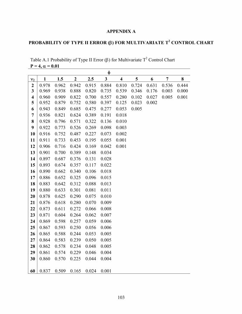
103
APPENDIX A
PROBABILITY OF TYPE II ERROR (β) FOR MULTIVARIATE T2 CONTROL CHART
Table A.1 Probability of Type II Error (β) for Multivariate T2 Control Chart P = 4, α = 0.01
φ ν2 1 1.5 2 2.5 3 4 5 6 7 8 2 0.978 0.962 0.942 0.915 0.884 0.810 0.724 0.631 0.536 0.444 3 0.969 0.938 0.888 0.820 0.735 0.539 0.346 0.176 0.003 0.000 4 0.960 0.909 0.822 0.700 0.557 0.280 0.102 0.027 0.005 0.001 5 0.952 0.879 0.752 0.580 0.397 0.125 0.023 0.002 6 0.943 0.849 0.685 0.475 0.277 0.053 0.005 7 0.936 0.821 0.624 0.389 0.191 0.018 8 0.928 0.796 0.571 0.322 0.136 0.010 9 0.922 0.773 0.526 0.269 0.098 0.003 10 0.916 0.752 0.487 0.227 0.073 0.002 11 0.911 0.733 0.453 0.195 0.055 0.001 12 0.906 0.716 0.424 0.169 0.042 0.001 13 0.901 0.700 0.389 0.148 0.034 14 0.897 0.687 0.376 0.131 0.028 15 0.893 0.674 0.357 0.117 0.022 16 0.890 0.662 0.340 0.106 0.018 17 0.886 0.652 0.325 0.096 0.015 18 0.883 0.642 0.312 0.088 0.013 19 0.880 0.633 0.301 0.081 0.011 20 0.878 0.625 0.290 0.075 0.010 21 0.876 0.618 0.280 0.070 0.009 22 0.873 0.611 0.272 0.066 0.008 23 0.871 0.604 0.264 0.062 0.007 24 0.869 0.598 0.257 0.059 0.006 25 0.867 0.593 0.250 0.056 0.006 26 0.865 0.588 0.244 0.053 0.005 27 0.864 0.583 0.239 0.050 0.005 28 0.862 0.578 0.234 0.048 0.005 29 0.861 0.574 0.229 0.046 0.004 30 0.860 0.570 0.225 0.044 0.004 60 0.837 0.509 0.165 0.024 0.001
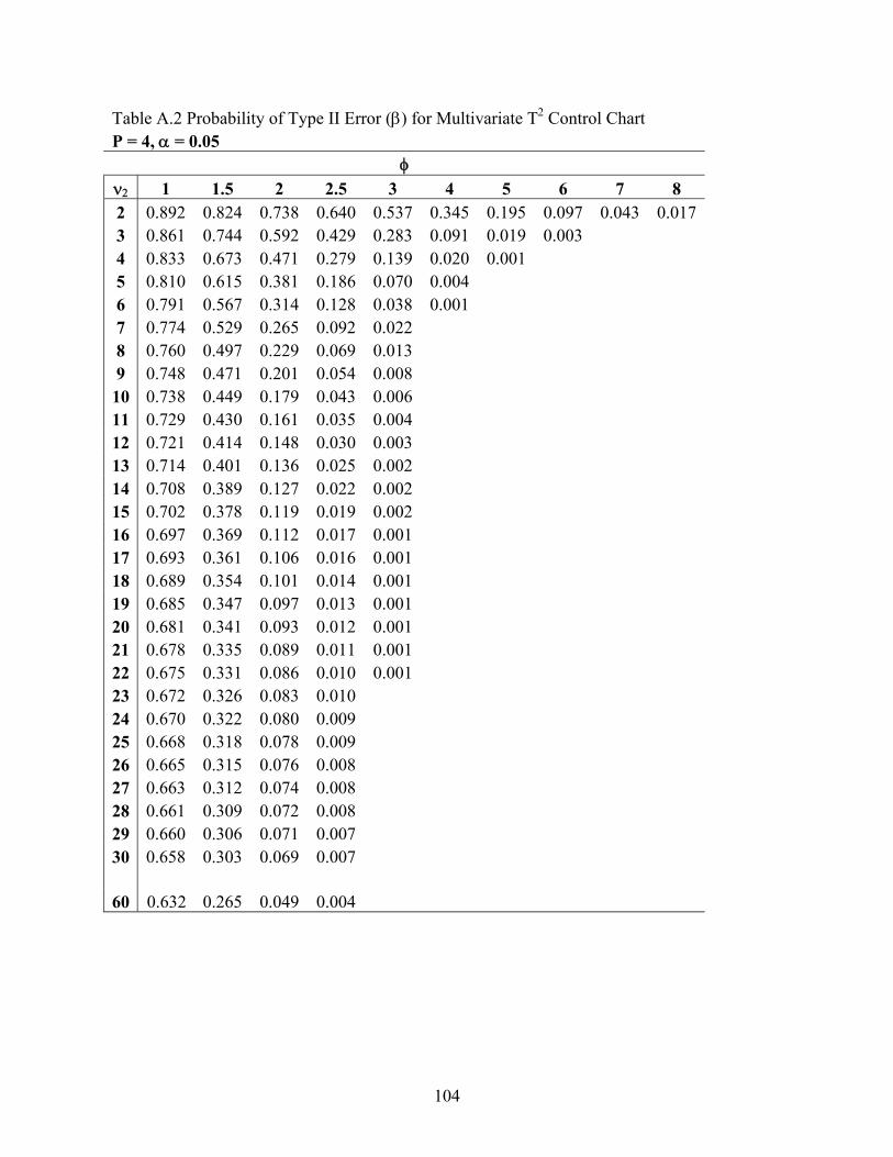
104
Table A.2 Probability of Type II Error (β) for Multivariate T2 Control Chart P = 4, α = 0.05
φ ν2 1 1.5 2 2.5 3 4 5 6 7 8 2 0.892 0.824 0.738 0.640 0.537 0.345 0.195 0.097 0.043 0.017 3 0.861 0.744 0.592 0.429 0.283 0.091 0.019 0.003 4 0.833 0.673 0.471 0.279 0.139 0.020 0.001 5 0.810 0.615 0.381 0.186 0.070 0.004 6 0.791 0.567 0.314 0.128 0.038 0.001 7 0.774 0.529 0.265 0.092 0.022 8 0.760 0.497 0.229 0.069 0.013 9 0.748 0.471 0.201 0.054 0.008 10 0.738 0.449 0.179 0.043 0.006 11 0.729 0.430 0.161 0.035 0.004 12 0.721 0.414 0.148 0.030 0.003 13 0.714 0.401 0.136 0.025 0.002 14 0.708 0.389 0.127 0.022 0.002 15 0.702 0.378 0.119 0.019 0.002 16 0.697 0.369 0.112 0.017 0.001 17 0.693 0.361 0.106 0.016 0.001 18 0.689 0.354 0.101 0.014 0.001 19 0.685 0.347 0.097 0.013 0.001 20 0.681 0.341 0.093 0.012 0.001 21 0.678 0.335 0.089 0.011 0.001 22 0.675 0.331 0.086 0.010 0.001 23 0.672 0.326 0.083 0.010 24 0.670 0.322 0.080 0.009 25 0.668 0.318 0.078 0.009 26 0.665 0.315 0.076 0.008 27 0.663 0.312 0.074 0.008 28 0.661 0.309 0.072 0.008 29 0.660 0.306 0.071 0.007 30 0.658 0.303 0.069 0.007 60 0.632 0.265 0.049 0.004
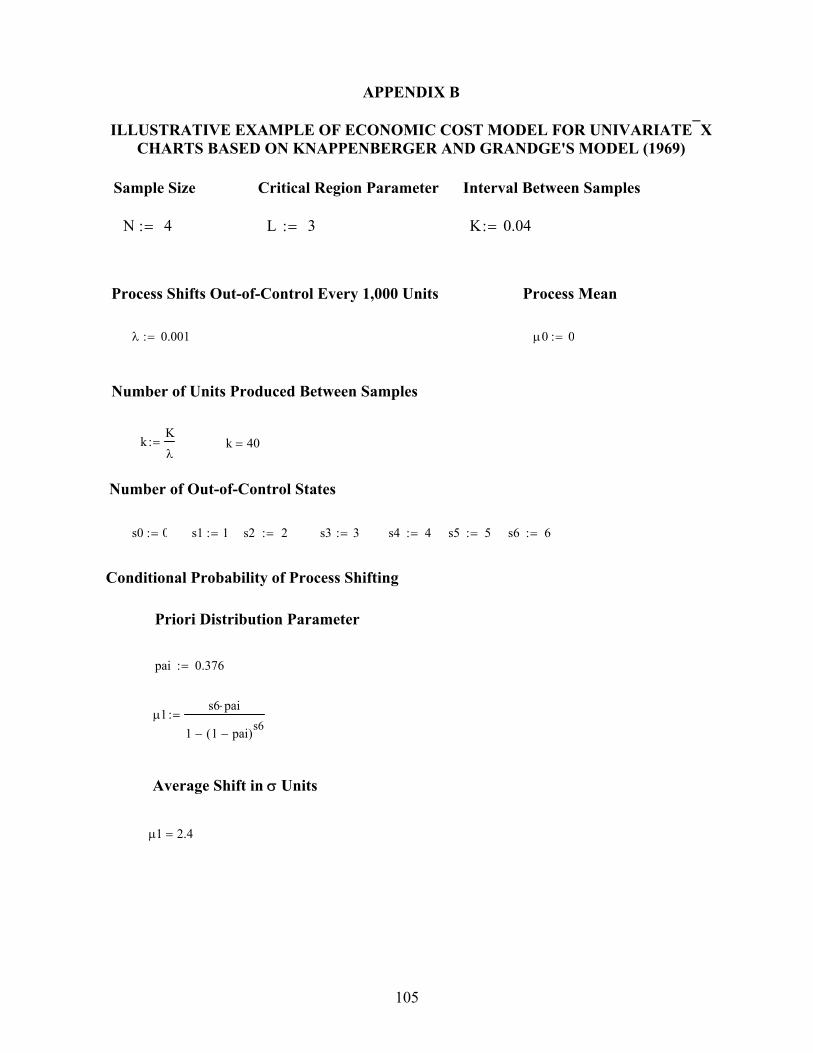
105
Sample Size
APPENDIX B
ILLUSTRATIVE EXAMPLE OF ECONOMIC COST MODEL FOR UNIVARIATE⎯X CHARTS BASED ON KNAPPENBERGER AND GRANDGE'S MODEL (1969)
Critical Region Parameter Interval Between Samples
Process Shifts Out-of-Control Every 1,000 Units Process Mean
λ 0.001:= μ0 0:=
Number of Units Produced Between Samples
kKλ
:= k 40=
Number of Out-of-Control States
s0 0:= s1 1:= s2 2:= s3 3:= s4 4:= s5 5:= s6 6:=
Conditional Probability of Process Shifting
Priori Distribution Parameter
pai 0.376:=
μ1s6 pai⋅
1 1 pai−( )s6−
:=
Average Shift in σ Units
μ1 2.4=
L 3:= K 0.04:=N 4:=

106
Conditional Probability of Producing a Defective Unit Given μ = μi (i = 1, 2... 6)
φ0 cnorm 3−( ) 2⋅:= φ1 cnorm 2−( ):= φ2 cnorm 1−( ):= φ3 cnorm 0( ):=
φ0 0.003= φ1 0.0228= φ2 0.1587= φ3 0.5=
φ4 cnorm 1( ):= φ5 cnorm 2( ):= φ6 cnorm 3( ):=
φ4 0.8413= φ5 0.9772= φ6 0.9987=
φ φ0 φ1 φ2 φ3 φ4 φ5 φ6( ):= φ 0.003 0.023 0.159 0.5 0.841 0.977 0.999( )=
Conditional Probability of Rejecting H0 Given that μ = μi
q0 cnorm s0 N⋅ L−( ) 2⋅:= q1 cnorm s1 N⋅ L−( ):= q2 cnorm s2 N⋅ L−( ):=
q0 0.003= q1 0.1587= q2 0.8413=
q3 cnorm s3 N⋅ L−( ):= q4 cnorm s4 N⋅ L−( ):= q5 cnorm s5 N⋅ L−( ):=
q3 0.9987= q4 1= q5 1=
q6 cnorm s6 N⋅ 3−( ):=
q6 1=
q q0 q1 q2 q3 q4 q5 q6( ):= q 0.003 0.159 0.841 0.999 1 1 1( )=

107
Probability that Process is in State μi at Time Test is Performed
p0 exp λ− k⋅( ):= p11 exp λ− k⋅( )−( ) s6!⋅ pai1⋅ 1 pai−( )s6 1−
⋅
1 1 pai−( )s6−⎡⎣ ⎤⎦ 1!⋅ s6 1−( )!⋅
:=
p0 0.9608= p1 0.009=
p21 exp λ− k⋅( )−( ) s6!⋅ pai2⋅ 1 pai−( )s6 2−
⋅
1 1 pai−( )s6−⎡⎣ ⎤⎦ 2!⋅ s6 2−( )!⋅
:= p31 exp λ− k⋅( )−( ) s6!⋅ pai3⋅ 1 pai−( )s6 3−
⋅
1 1 pai−( )s6−⎡⎣ ⎤⎦ 3!⋅ s6 3−( )!⋅
:=
p2 0.013= p3 0.011=
p41 exp λ− k⋅( )−( ) s6!⋅ pai4⋅ 1 pai−( )s6 4−
⋅
1 1 pai−( )s6−⎡⎣ ⎤⎦ 4!⋅ s6 4−( )!⋅
:= p51 exp λ− k⋅( )−( ) s6!⋅ pai5⋅ 1 pai−( )s6 5−
⋅
1 1 pai−( )s6−⎡⎣ ⎤⎦ 5!⋅ s6 5−( )!⋅
:=
p4 0.005= p5 0.001=
p61 exp λ− k⋅( )−( ) s6!⋅ pai6⋅ 1 pai−( )s6 6−
⋅
1 1 pai−( )s6−⎡⎣ ⎤⎦ 6!⋅ s6 6−( )!⋅
:=
p6 0=
p p0 p1 p2 p3 p4 p5 p6( ):= p 0.9610.0090.0130.0110.0050.0010( )=
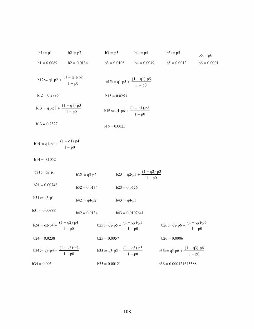
108
b1 p1:= b2 p2:= b3 p3:= b4 p4:= b5 p5:= b6 p6:=
b1 0.0089= b2 0.0134= b3 0.0108= b4 0.0049= b5 0.0012= b6 0.0001=
b12 q1 p2⋅1 q1−( ) p2⋅
1 p0−+:= b15 q1 p5⋅
1 q1−( ) p5⋅
1 p0−+:=
b12 0.2896= b15 0.0253=
b13 q1 p3⋅1 q1−( ) p3⋅
1 p0−+:=
b16 q1 p6⋅1 q1−( ) p6⋅
1 p0−+:=
b13 0.2327= b16 0.0025=
b14 q1 p4⋅1 q1−( ) p4⋅
1 p0−+:=
b14 0.1052=
b21 q2 p1⋅:= b32 q3 p2⋅:= b23 q2 p3⋅
1 q2−( ) p3⋅
1 p0−+:=
b21 0.00748= b32 0.0134= b23 0.0526=
b31 q3 p1⋅:= b42 q4 p2⋅:= b43 q4 p3⋅:=
b31 0.00888= b42 0.0134= b43 0.0107641=
b24 q2 p4⋅1 q2−( ) p4⋅
1 p0−+:= b25 q2 p5⋅
1 q2−( ) p5⋅
1 p0−+:= b26 q2 p6⋅
1 q2−( ) p6⋅
1 p0−+:=
b24 0.0238= b25 0.0057= b26 0.0006=
b34 q3 p4⋅1 q3−( ) p4⋅
1 p0−+:= b35 q3 p5⋅
1 q3−( ) p5⋅
1 p0−+:= b36 q3 p6⋅
1 q3−( ) p6⋅
1 p0−+:=
b34 0.005= b35 0.00121= b36 0.000121643588=
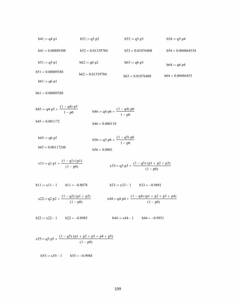
109
b41 q4 p1⋅:= b52 q5 p2⋅:= b53 q5 p3⋅:= b54 q5 p4⋅:=
b41 0.00889388= b52 0.01339784= b53 0.01076408= b54 0.004864534=
b51 q5 p1⋅:= b62 q6 p2⋅:= b63 q6 p3⋅:= b64 q6 p4⋅:= b51 0.00889388=
b62 0.01339784= b64 0.00486453=b63 0.01076408=b61 q6 p1⋅:=
b61 0.00889388=
b45 q4 p5⋅1 q4−( ) p5⋅
1 p0−+:=
b46 q4 p6⋅1 q4−( ) p6⋅
1 p0−+:=
b45 0.001172= b46 0.000118=
b65 q6 p5⋅:= b56 q5 p6⋅1 q5−( ) p6⋅
1 p0−+:=
b65 0.00117248= b56 0.0001=
x11 q1 p1⋅1 q1−( ) p1( )⋅
1 p0−( )+:=
x33 q3 p3⋅1 q3−( ) p1 p2+ p3+( )⋅
1 p0−( )+:=
b11 x11 1−:= b11 0.8078−= b33 x33 1−:= b33 0.9881−=
x22 q2 p2⋅1 q2−( ) p1 p2+( )⋅
1 p0−( )+:= x44 q4 p4⋅
1 q4−( ) p1 p2+ p3+ p4+( )⋅
1 p0−( )+:=
b22 x22 1−:= b22 0.8985−= b44 x44 1−:= b44 0.9951−=
x55 q5 p5⋅1 q5−( ) p1 p2+ p3+ p4+ p5+( )⋅
1 p0−( )+:=
b55 x55 1−:= b55 0.9988−=
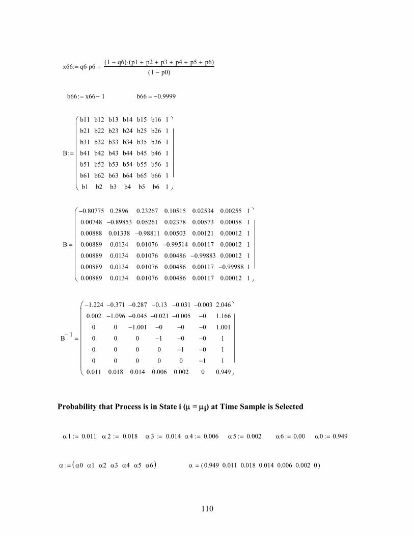
110
x66 q6 p6⋅
1 q6−( ) p1 p2+ p3+ p4+ p5+ p6+( )⋅
1 p0−( )+:=
b66 x66 1−:= b66 0.9999−=
B
b11
b21
b31
b41
b51
b61
b1
b12
b22
b32
b42
b52
b62
b2
b13
b23
b33
b43
b53
b63
b3
b14
b24
b34
b44
b54
b64
b4
b15
b25
b35
b45
b55
b65
b5
b16
b26
b36
b46
b56
b66
b6
1
1
1
1
1
1
1
⎛⎜⎜⎜⎜⎜⎜⎜⎜⎝
⎞⎟⎟⎟⎟⎟⎟⎟⎟⎠
:=
B
0.80775−
0.00748
0.00888
0.00889
0.00889
0.00889
0.00889
0.2896
0.89853−
0.01338
0.0134
0.0134
0.0134
0.0134
0.23267
0.05261
0.98811−
0.01076
0.01076
0.01076
0.01076
0.10515
0.02378
0.00503
0.99514−
0.00486
0.00486
0.00486
0.02534
0.00573
0.00121
0.00117
0.99883−
0.00117
0.00117
0.00255
0.00058
0.00012
0.00012
0.00012
0.99988−
0.00012
1
1
1
1
1
1
1
⎛⎜⎜⎜⎜⎜⎜⎜⎜⎝
⎞⎟⎟⎟⎟⎟⎟⎟⎟⎠
=
B 1−
1.224−
0.002
0
0
0
0
0.011
0.371−
1.096−
0
0
0
0
0.018
0.287−
0.045−
1.001−
0
0
0
0.014
0.13−
0.021−
0−
1−
0
0
0.006
0.031−
0.005−
0−
0−
1−
0
0.002
0.003−
0−
0−
0−
0−
1−
0
2.046
1.166
1.001
1
1
1
0.949
⎛⎜⎜⎜⎜⎜⎜⎜⎜⎝
⎞⎟⎟⎟⎟⎟⎟⎟⎟⎠
=
Probability that Process is in State i (μ = μi) at Time Sample is Selected
α1 0.011:= α 2 0.018:= α 3 0.014:= α4 0.006:= α5 0.002:= α6 0.00:= α0 0.949:=
α α0 α1 α2 α3 α4 α5 α6( ):= α 0.949 0.011 0.018 0.014 0.006 0.002 0( )=

111
Conditional Expectation of Occurrence of Assignable Cause Within an Interval of Sampling
F1 1 λ k⋅+( ) exp λ− k⋅( )⋅−⎡⎣ ⎤⎦
λ k⋅ 1 exp λ− k⋅( )−( )⋅:=
F 0.4967=
γ0 α0 p0⋅ F α0⋅ 1 p0−( )⋅+:=
γ0 0.9303=
x1 α1p1( )
1 p0−⋅:= y1 α2
p1 p2+( )1 p0−
⋅:= y1 0.01=x1 0.002=
x2 α0 1 F−( )⋅ p1⋅:= x2 0.004= y2 α0 1 F−( )⋅ p2⋅:=
y2 0.006=
x3 α1p0
1 p0−⎛⎜⎝
⎞⎟⎠
⋅ 1 F−( )⋅:= x3 0.1357=
y3 α1p2
1 p0−⎛⎜⎝
⎞⎟⎠
⋅ 1 F−( )⋅⎡⎢⎣
⎤⎥⎦
:=
x4α1 F⋅
1 p0−⎛⎜⎝
⎞⎟⎠
p2 p3+ p4+ p5+ p6+( )⋅:= x4 0.004=y3 0.002=
γ1 x1 x2+ x4+:= y4α2 F⋅
1 p0−⎛⎜⎝
⎞⎟⎠
p3 p4+ p5+ p6+( )⋅:=
y4 0.004=γ1 0.011=
γ2 y1 y2+ y3+ y4+:=
γ2 0.0224=
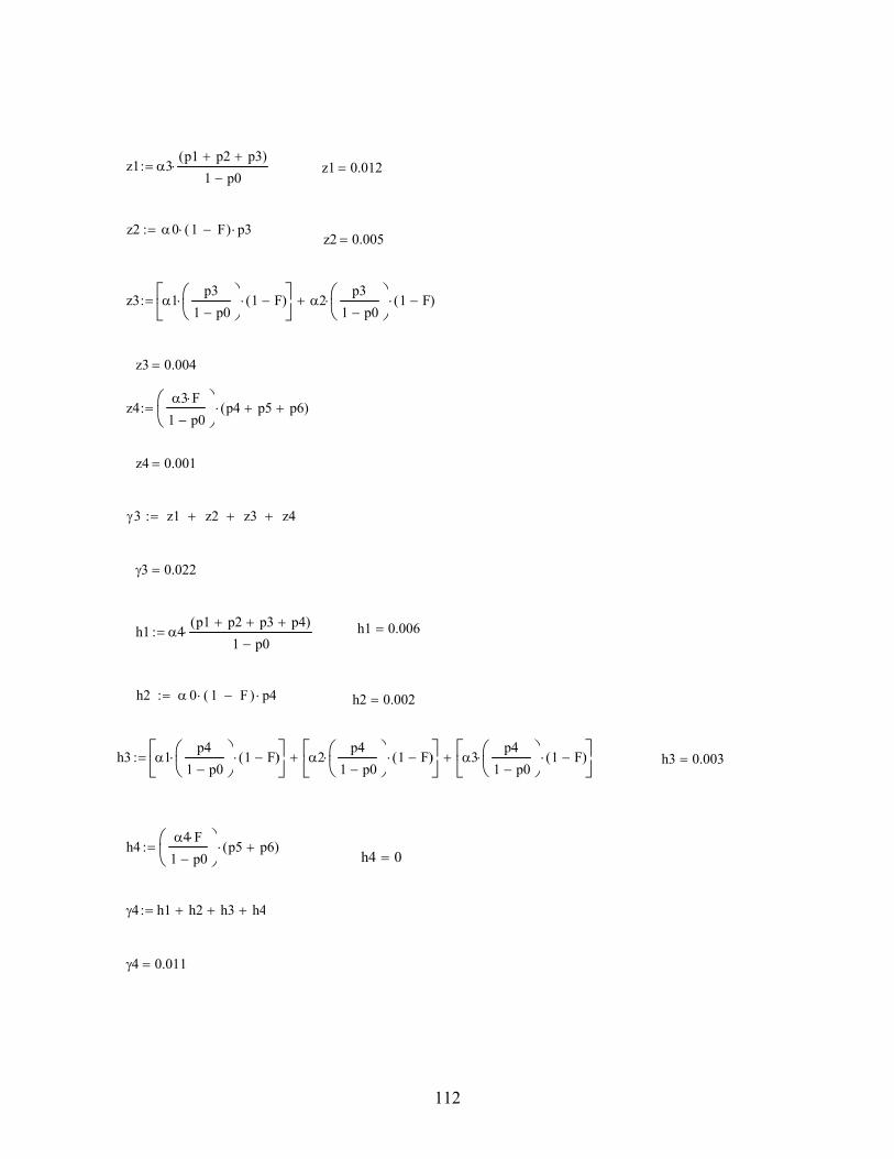
112
z1 α3p1 p2+ p3+( )
1 p0−⋅:= z1 0.012=
z2 α0 1 F−( )⋅ p3⋅:= z2 0.005=
z3 α1p3
1 p0−⎛⎜⎝
⎞⎟⎠
⋅ 1 F−( )⋅⎡⎢⎣
⎤⎥⎦
α2p3
1 p0−⎛⎜⎝
⎞⎟⎠
⋅ 1 F−( )⋅+:=
z3 0.004=
z4α3 F⋅
1 p0−⎛⎜⎝
⎞⎟⎠
p4 p5+ p6+( )⋅:=
z4 0.001=
γ3 z1 z2+ z3+ z4+:=
γ3 0.022=
h1 α4p1 p2+ p3+ p4+( )
1 p0−⋅:= h1 0.006=
h2 α 0 1 F−( )⋅ p4⋅:= h2 0.002=
h3 α1p4
1 p0−⎛⎜⎝
⎞⎟⎠
⋅ 1 F−( )⋅⎡⎢⎣
⎤⎥⎦
α2p4
1 p0−⎛⎜⎝
⎞⎟⎠
⋅ 1 F−( )⋅⎡⎢⎣
⎤⎥⎦
+ α3p4
1 p0−⎛⎜⎝
⎞⎟⎠
⋅ 1 F−( )⋅⎡⎢⎣
⎤⎥⎦
+:= h3 0.003=
h4α4 F⋅
1 p0−⎛⎜⎝
⎞⎟⎠
p5 p6+( )⋅:= h4 0=
γ4 h1 h2+ h3+ h4+:=
γ4 0.011=
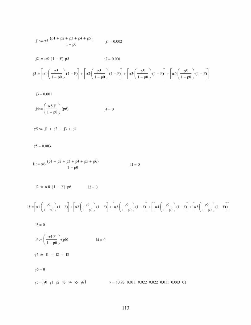
113
j1 α5p1 p2+ p3+ p4+ p5+( )
1 p0−⋅:= j1 0.002=
j2 α0 1 F−( )⋅ p5⋅:= j2 0.001=
j3 α1p5
1 p0−⎛⎜⎝
⎞⎟⎠
⋅ 1 F−( )⋅⎡⎢⎣
⎤⎥⎦
α2p5
1 p0−⎛⎜⎝
⎞⎟⎠
⋅ 1 F−( )⋅⎡⎢⎣
⎤⎥⎦
+ α3p5
1 p0−⎛⎜⎝
⎞⎟⎠
⋅ 1 F−( )⋅⎡⎢⎣
⎤⎥⎦
+ α4p5
1 p0−⎛⎜⎝
⎞⎟⎠
⋅ 1 F−( )⋅⎡⎢⎣
⎤⎥⎦
+:=
j3 0.001=
j4α5 F⋅
1 p0−⎛⎜⎝
⎞⎟⎠
p6( )⋅:= j4 0=
γ5 j1 j2+ j3+ j4+:=
γ5 0.003=
l1 α6p1 p2+ p3+ p4+ p5+ p6+( )
1 p0−⋅:= l1 0=
l2 α0 1 F−( )⋅ p6⋅:= l2 0=
l3 α1p6
1 p0−⎛⎜⎝
⎞⎟⎠
⋅ 1 F−( )⋅⎡⎢⎣
⎤⎥⎦
α2p6
1 p0−⎛⎜⎝
⎞⎟⎠
⋅ 1 F−( )⋅⎡⎢⎣
⎤⎥⎦
+ α3p6
1 p0−⎛⎜⎝
⎞⎟⎠
⋅ 1 F−( )⋅⎡⎢⎣
⎤⎥⎦
+ α4p6
1 p0−⎛⎜⎝
⎞⎟⎠
⋅ 1 F−( )⋅⎡⎢⎣
⎤⎥⎦
α5p6
1 p0−⎛⎜⎝
⎞⎟⎠
⋅ 1 F−( )⋅⎡⎢⎣
⎤⎥⎦
+⎡⎢⎣
⎤⎥⎦
+:=
l3 0=
l4α4 F⋅
1 p0−⎛⎜⎝
⎞⎟⎠
p6( )⋅:= l4 0=
γ6 l1 l2+ l3+:=
γ6 0=
γ γ0 γ1 γ2 γ3 γ4 γ5 γ6( ):= γ 0.93 0.011 0.022 0.022 0.011 0.003 0( )=
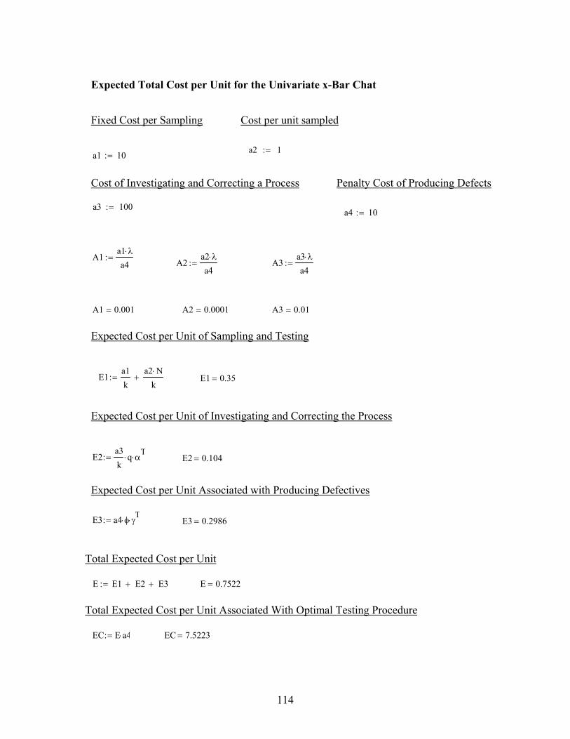
114
Expected Total Cost per Unit for the Univariate x-Bar Chat
Fixed Cost per Sampling Cost per unit sampled
a2 1:=a1 10:=
Cost of Investigating and Correcting a Process Penalty Cost of Producing Defects
a3 100:= a4 10:=
A1a1 λ⋅
a4:=
A2a2 λ⋅
a4:= A3
a3 λ⋅
a4:=
A1 0.001= A2 0.0001= A3 0.01=
Expected Cost per Unit of Sampling and Testing
E1a1k
a2 N⋅
k+:= E1 0.35=
Expected Cost per Unit of Investigating and Correcting the Process
E2a3k
q⋅ αT
⋅:= E2 0.104=
Expected Cost per Unit Associated with Producing Defectives
E3 a4 φ⋅ γT
⋅:= E3 0.2986=
Total Expected Cost per Unit
E E1 E2+ E3+:= E 0.7522=
Total Expected Cost per Unit Associated With Optimal Testing Procedure
EC E a4⋅:= EC 7.5223=

115
APPENDIX C
ILLUSTRATIVE EXAMPLE OF ECONOMIC COST MODEL FOR MULTIVARIATE T2 CHARTS BASED ON MONTGOMERY AND KLATT'S
MODEL (1972)
a1 1:= a2 10:= a3 1000:= a4 1:= λ' .0001:=
A1a1 λ'( )⋅⎡⎣ ⎤⎦
a4:= A2
a2 λ'( )⋅⎡⎣ ⎤⎦a4
:= A3a3 λ'( )⋅⎡⎣ ⎤⎦
a4:=
A1 0.0001= A2 0.001= A3 0.1=
N 10:= K .15:= kKλ'
:= k 1500=
Probability of Remaining in the State of μ0, while k Units are Produced
P0 exp λ'− k⋅( ):= P0 0.861=
Probability of out-of-control State of μ1, while k Units are Produced
P1 1 P0−:= P1 0.139=
Subgroup Size Delta Shift in the Mean
n N 1−:= δ5
6⎛⎜⎝
⎞⎟⎠
:=
S1sq 2:= S12 1:=
S2sq 2.5:=
Variance Covariance Matrix
ΣS1sq
S12
S12
S2sq⎛⎜⎝
⎞⎟⎠
:= Σ
2
1
1
2.5⎛⎜⎝
⎞⎟⎠
=
Correlation Coefficient
rS12
S1sq S2sq⋅:=
r 0.447=
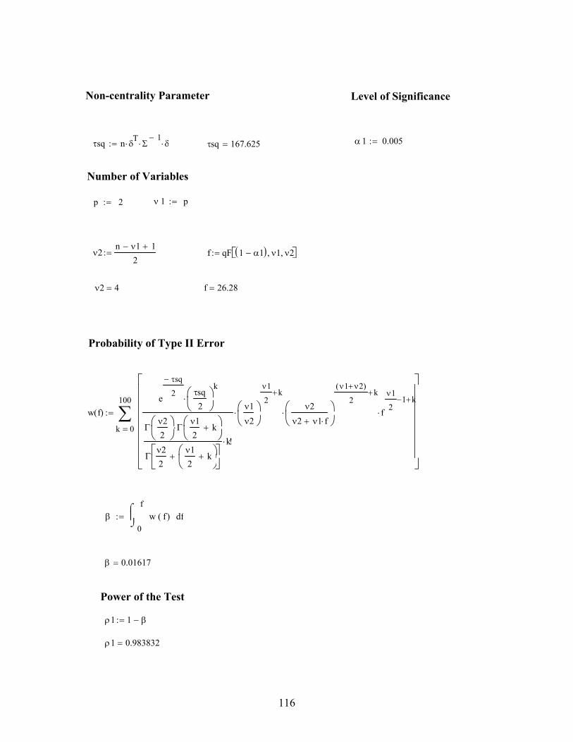
116
Non-centrality Parameter Level of Significance
τsq n δT
⋅ Σ1−
⋅ δ⋅:= τsq 167.625= α 1 0.005:=
Number of Variables
p 2:= ν 1 p:=
ν2n ν1− 1+
2:= f qF 1 α1−( ) ν1, ν2,⎡⎣ ⎤⎦:=
f 26.28=ν2 4=
Probability of Type II Error
w f( )
0
100
k
e
τsq−
2 τsq2
⎛⎜⎝
⎞⎟⎠
k⋅
Γν22
⎛⎜⎝
⎞⎟⎠
Γν12
k+⎛⎜⎝
⎞⎟⎠
⋅
Γν22
ν12
k+⎛⎜⎝
⎞⎟⎠
+⎡⎢⎣
⎤⎥⎦
k!⋅
ν1ν2
⎛⎜⎝
⎞⎟⎠
ν1
2k+
⋅ν2
ν2 ν1 f⋅+⎛⎜⎝
⎞⎟⎠
ν1 ν2+( )
2k+
⋅ f
ν1
21− k+
⋅
⎡⎢⎢⎢⎢⎢⎢⎢⎣
⎤⎥⎥⎥⎥⎥⎥⎥⎦
∑=
:=
β0
ffw f( )
⌠⎮⌡
d:=
β 0.01617=
Power of the Test
ρ1 1 β−:=
ρ1 0.983832=
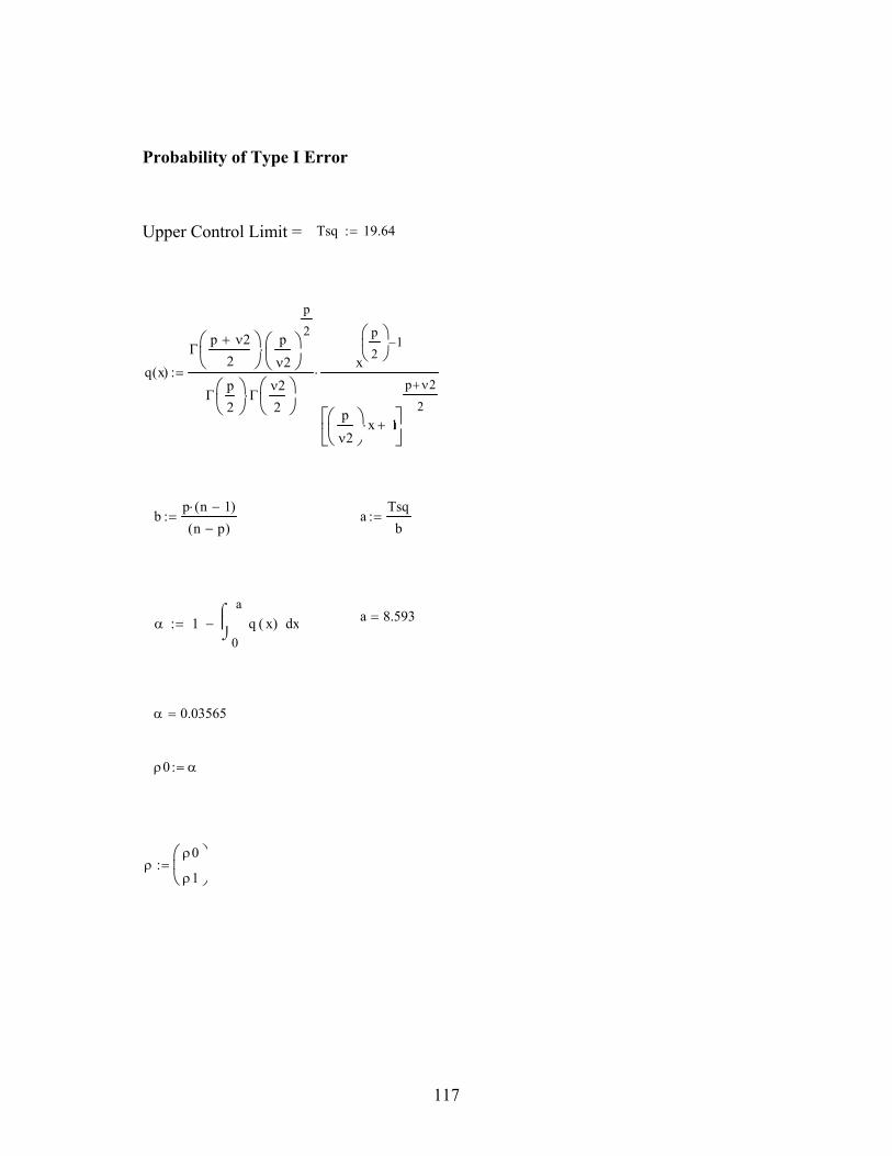
117
Probability of Type I Error
Upper Control Limit = Tsq 19.64:=
q x( )Γ
p ν2+
2⎛⎜⎝
⎞⎟⎠
pν2
⎛⎜⎝
⎞⎟⎠
p
2⋅
Γp2
⎛⎜⎝
⎞⎟⎠
Γν22
⎛⎜⎝
⎞⎟⎠
⋅
x
p
2⎛⎜⎝
⎞⎟⎠
1−
pν2
⎛⎜⎝
⎞⎟⎠
x⋅ 1+⎡⎢⎣
⎤⎥⎦
p ν2+
2
⋅:=
bp n 1−( )⋅
n p−( ):= a
Tsqb
:=
a 8.593=α 10
axq x( )
⌠⎮⌡
d−:=
α 0.03565=
ρ0 α:=
ρρ0
ρ1⎛⎜⎝
⎞⎟⎠
:=
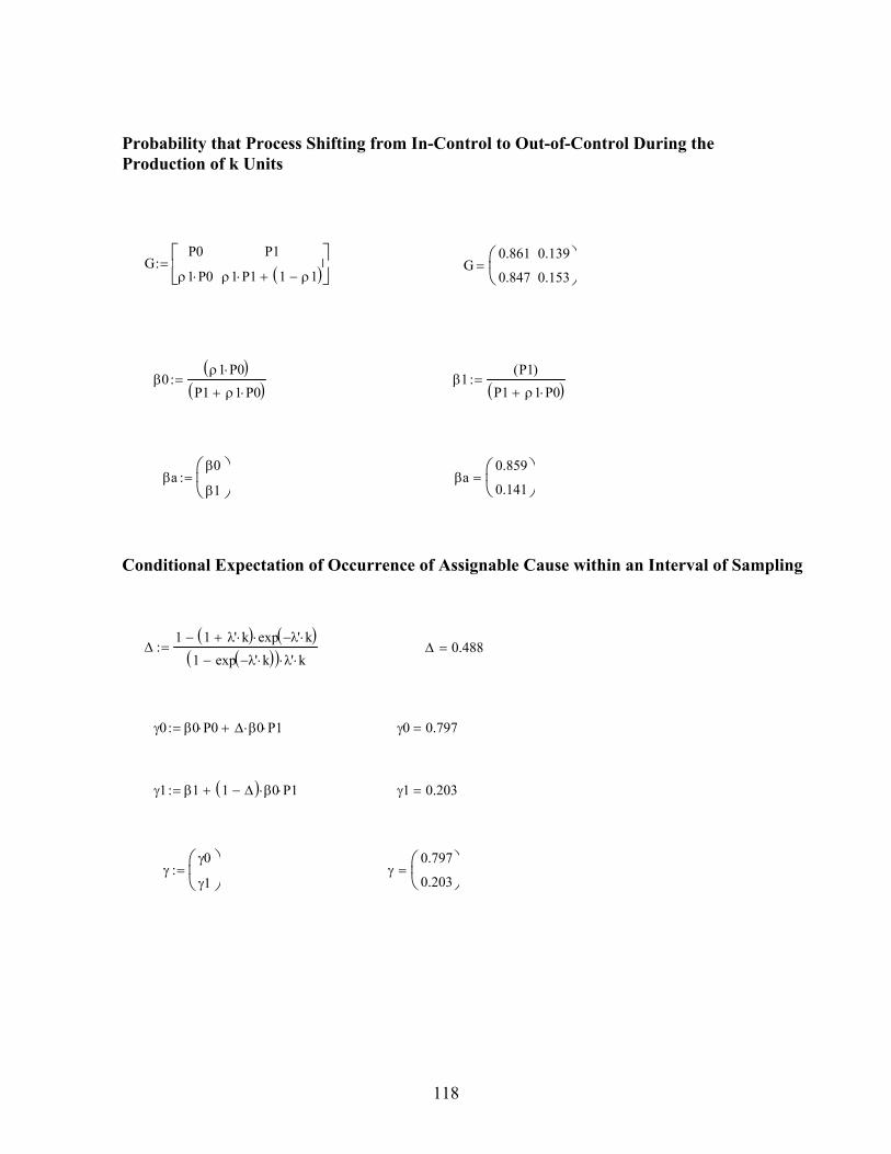
118
Probability that Process Shifting from In-Control to Out-of-Control During the Production of k Units
GP0
ρ1 P0⋅
P1
ρ1 P1⋅ 1 ρ1−( )+
⎡⎢⎣
⎤⎥⎦
:= G0.861
0.847
0.139
0.153⎛⎜⎝
⎞⎟⎠
=
β0ρ1 P0⋅( )
P1 ρ1 P0⋅+( ):= β1P1( )
P1 ρ1 P0⋅+( ):=
βaβ0
β1⎛⎜⎝
⎞⎟⎠
:= βa0.859
0.141⎛⎜⎝
⎞⎟⎠
=
Conditional Expectation of Occurrence of Assignable Cause within an Interval of Sampling
Δ1 1 λ' k⋅+( ) exp λ'− k⋅( )⋅−
1 exp λ'− k⋅( )−( ) λ'⋅ k⋅:= Δ 0.488=
γ0 β0 P0⋅ Δ β0⋅ P1⋅+:= γ0 0.797=
γ1 β1 1 Δ−( ) β0⋅ P1⋅+:= γ1 0.203=
γγ0
γ1⎛⎜⎝
⎞⎟⎠
:= γ0.797
0.203⎛⎜⎝
⎞⎟⎠
=
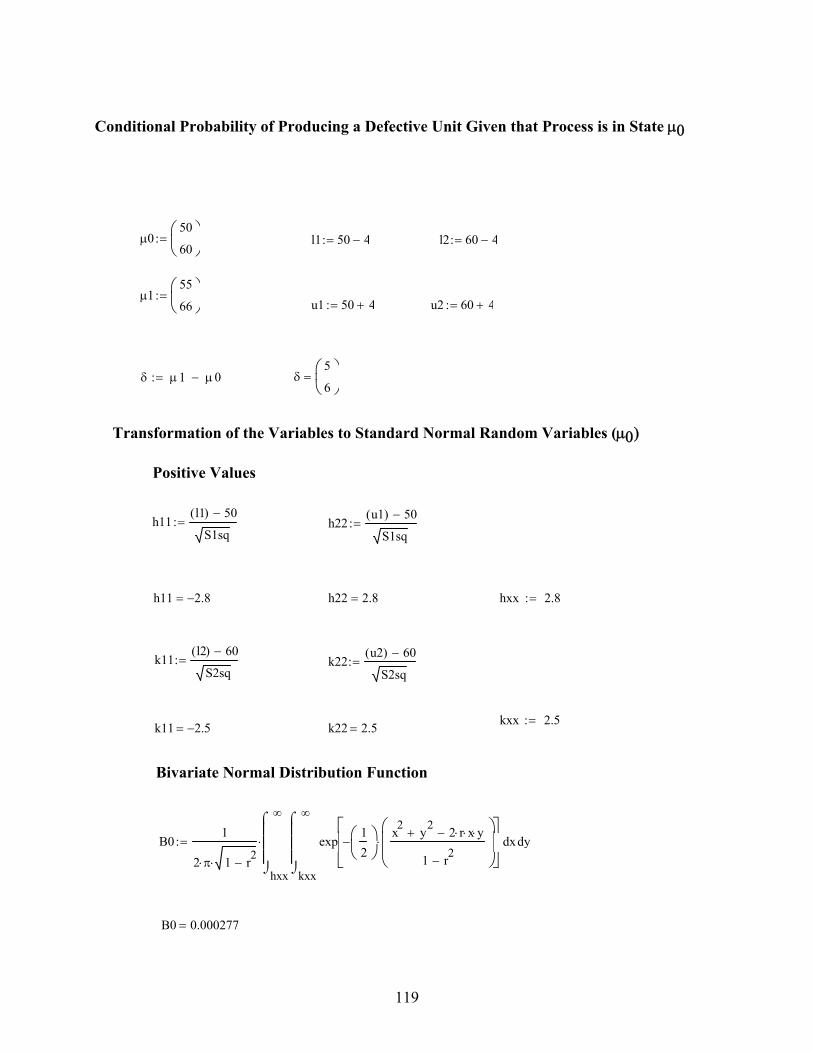
119
Conditional Probability of Producing a Defective Unit Given that Process is in State μ0
μ050
60⎛⎜⎝
⎞⎟⎠
:= l1 50 4−:= l2 60 4−:=
μ155
66⎛⎜⎝
⎞⎟⎠
:= u1 50 4+:= u2 60 4+:=
δ μ1 μ0−:= δ5
6⎛⎜⎝
⎞⎟⎠
=
Transformation of the Variables to Standard Normal Random Variables (μ0)
Positive Values
h11l1( ) 50−
S1sq:= h22
u1( ) 50−
S1sq:=
h11 2.8−= h22 2.8= hxx 2.8:=
k11l2( ) 60−
S2sq:= k22
u2( ) 60−
S2sq:=
kxx 2.5:=k11 2.5−= k22 2.5=
Bivariate Normal Distribution Function
B01
2 π⋅ 1 r2−⋅hxx
∞
y
kxx
∞
xexp12
⎛⎜⎝
⎞⎟⎠
−x2 y2
+ 2 r⋅ x⋅ y⋅−
1 r2−
⎛⎜⎜⎝
⎞⎟⎟⎠
⋅⎡⎢⎢⎣
⎤⎥⎥⎦
⌠⎮⎮⎮⌡
d
⌠⎮⎮⎮⌡
d⋅:=
B0 0.000277=
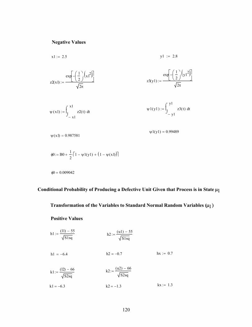
120
Negative Values
x1 2.5:= y1 2.8:=
z2 x1( )exp
12
⎛⎜⎝
⎞⎟⎠
− x12( )⋅⎡⎢⎣
⎤⎥⎦
2π:= z3 y1( )
exp12
⎛⎜⎝
⎞⎟⎠
− y12( )⋅⎡⎢⎣
⎤⎥⎦
2π:=
ψ1 y1( )y1−
y1tz3 t( )
⌠⎮⌡
d:= ψ x1( )
x1−
x1tz2 t( )
⌠⎮⌡
d:=
ψ1 y1( ) 0.99489= ψ x1( ) 0.987581=
φ0 B012
1 ψ1 y1( )− 1 ψ x1( )−( )+⎡⎣ ⎤⎦⋅+:=
φ0 0.009042=
Conditional Probability of Producing a Defective Unit Given that Process is in State μ1
Transformation of the Variables to Standard Normal Random Variables (μ1)
Positive Values
h1l1( ) 55−
S1sq:= h2
u1( ) 55−
S1sq:=
h1 6.4−= h2 0.7−= hx 0.7:=
k1l2( ) 66−
S2sq:= k2
u2( ) 66−
S2sq:=
kx 1.3:=k1 6.3−= k2 1.3−=
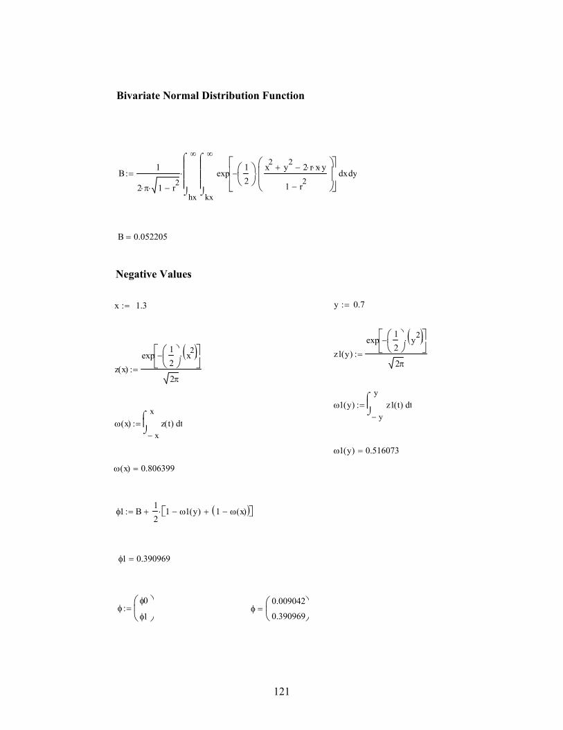
121
Bivariate Normal Distribution Function
B1
2 π⋅ 1 r2−⋅hx
∞
y
kx
∞
xexp12
⎛⎜⎝
⎞⎟⎠
−x2 y2
+ 2 r⋅ x⋅ y⋅−
1 r2−
⎛⎜⎜⎝
⎞⎟⎟⎠
⋅⎡⎢⎢⎣
⎤⎥⎥⎦
⌠⎮⎮⎮⌡
d
⌠⎮⎮⎮⌡
d⋅:=
B 0.052205=
Negative Values
x 1.3:= y 0.7:=
z1 y( )exp
12
⎛⎜⎝
⎞⎟⎠
− y2( )⋅⎡⎢⎣
⎤⎥⎦
2π:=
z x( )exp
12
⎛⎜⎝
⎞⎟⎠
− x2( )⋅⎡⎢⎣
⎤⎥⎦
2π:=
ω1 y( )y−
ytz1 t( )
⌠⎮⌡
d:=
ω x( )x−
xtz t( )
⌠⎮⌡
d:=
ω1 y( ) 0.516073=
ω x( ) 0.806399=
φ1 B12
1 ω1 y( )− 1 ω x( )−( )+⎡⎣ ⎤⎦⋅+:=
φ1 0.390969=
φφ0
φ1⎛⎜⎝
⎞⎟⎠
:= φ0.009042
0.390969⎛⎜⎝
⎞⎟⎠
=
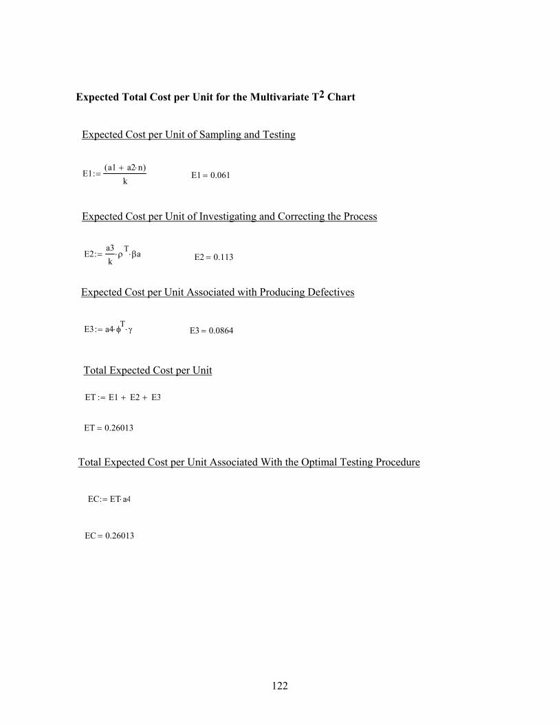
122
Expected Total Cost per Unit for the Multivariate T2 Chart
Expected Cost per Unit of Sampling and Testing
E1a1 a2 n⋅+( )
k:= E1 0.061=
Expected Cost per Unit of Investigating and Correcting the Process
E2a3k
ρT
⋅ βa⋅:= E2 0.113=
Expected Cost per Unit Associated with Producing Defectives
E3 a4 φT
⋅ γ⋅:= E3 0.0864=
Total Expected Cost per Unit
ET E1 E2+ E3+:=
ET 0.26013=
Total Expected Cost per Unit Associated With the Optimal Testing Procedure
EC ET a4⋅:=
EC 0.26013=