Embed Size (px)
Citation preview

Multivariate Multilevel Models
for Longitudinal Data
(in SAS and Mplus)
CLP 945: Lecture 9 1
• Topics:
Univariate vs. multivariate approaches for modeling
time-varying (or any lower-level) predictors
Multivariate relations of change (per level of analysis)
Multivariate tests of differences in effect size and
their specification in univariate MLM software
What not to do: smushed effects path models
for longitudinal data
Single-level SEM for multivariate multilevel models

Univariate MLM for Specifying Time-Varying Predictors
• “Univariate” approach to MLM is appropriate for time-varying predictors that fluctuate over time (and lower-level predictors with only mean differences across higher levels in general)
• Level-1 predictor can be created two different ways:
Easier to understand is variable-based-centering: 𝐖𝐏𝐱𝐭𝐢 = 𝐱𝐭𝐢 − 𝐗 𝐢
Directly isolates level-1 within variance, so 𝐖𝐏𝐱𝐭𝐢 within effects
More common is constant-based-centering: 𝐓𝐕𝐱𝐭𝐢 = 𝐱𝐭𝐢 − 𝑪
Does NOT isolate level-1 within variance, so 𝐓𝐕𝐱𝐭𝐢 will have smushed between/within effects unless it is paired with level-2 predictor analog
• Level-2 predictor is always constant-centered: 𝐏𝐌𝐱𝐢 = 𝐗 𝐢 − 𝑪
𝐏𝐌𝐱𝐢 indicates total between effect when paired with 𝐖𝐏𝐱𝐭𝐢
𝐏𝐌𝐱𝐢 indicates contextual between effect when paired with 𝐓𝐕𝐱𝐭𝐢
Within + Contextual Between = Total Between
CLP 945: Lecture 9 2

Univariate: Constant-Based Centering
Without Level-2 Predictor = Smushing
CLP 945: Lecture 9 3
𝐲𝐭𝐢
L2 BP
Intercept
Variance
(of 𝐔𝟎𝐢𝐲)
L1 WP
Residual
Variance
(of 𝐞𝐭𝐢𝐱)
Smushed
effect γ10
𝐱𝐭𝐢
Constant-centered level-1 𝐱𝐭𝐢 has
not been partitioned – AND – it
has only one fixed effect in the
model. Thus, that smushed effect
reflects equal BP and WP effects.
Smushed
effect γ10
Model-based partitioning
of level-1 yti outcome
variance into
variance components:
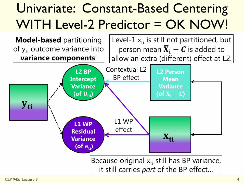
Univariate: Constant-Based Centering
WITH Level-2 Predictor = OK NOW!
CLP 945: Lecture 9 4
𝐲𝐭𝐢
L2 BP
Intercept
Variance
(of 𝐔𝟎𝐢)
L1 WP
Residual
Variance
(of 𝐞𝐭𝐢)
L2 Person
Mean
Variance
(of 𝐗 𝐢 − 𝑪)
Model-based partitioning
of yti outcome variance into
variance components:
Contextual L2
BP effect
L1 WP
effect 𝐱𝐭𝐢
Level-1 xti is still not partitioned, but
person mean 𝐗 𝐢 − 𝑪 is added to
allow an extra (different) effect at L2.
Because original xti still has BP variance,
it still carries part of the BP effect…

Univariate: Variable-Based-Centering
CLP 945: Lecture 9 5
𝐲𝐭𝐢
L2 BP
Intercept
Variance
(of 𝐔𝟎𝐢𝐲)
L1 WP
Residual
Variance
(of 𝐞𝐭𝐢𝐲)
L2 Person
Mean
Variance
(of 𝐗 𝐢 − 𝑪)
L1 WP
Deviation
Variance
(of 𝐱𝐭𝐢 − 𝐗 𝐢 )
Model-based partitioning
of level-1 yti outcome
variance into
variance components:
Brute-force partitioning
of level-1 xti predictor variance
into observed variables:
Why not let the model make variance components for xti, too?
This is the basis of multivariate MLM (or “multilevel SEM” = M-SEM).
L2 BP
effect γ01
L1 WP
effect γ10
𝐱𝐭𝐢

“Truly” Multivariate Multilevel Modeling
CLP 945: Lecture 9 6
𝐲𝐭𝐢
L2 BP
Intercept
Variance
(of 𝐔𝟎𝐢𝐲)
L1 WP
Residual
Variance
(of 𝐞𝐭𝐢𝐲)
Model-based partitioning
of level-1 yti outcome
variance into
variance components:
L2 BP
effect γ01
L1 WP
effect γ10
𝐱𝐭𝐢
Model-based partitioning
of level-1 xti outcome
variance into
variance components:
L2 BP
Intercept
Variance
(of 𝐔𝟎𝐢𝐱)
L1 WP
Residual
Variance
(of 𝐞𝐭𝐢𝐱)
Univariate MLM software can do multivariate MLM if the relationships
between X and Y at each level are phrased as covariances, but if you
want directed regressions (or moderators thereof), you need “M-SEM”

Univariate vs. Truly Multivariate MLM • If your time-varying predictors have only BP intercept variance, their piles
of variance can be reasonably approximated in univariate MLM OR by truly multivariate MLMs (so-called Multilevel SEM, or M-SEM)
It’s called “SEM” because random effects = latent variables, but there is no latent variable measurement model as in traditional SEM, so that’s why I don’t like the term M-SEM, and prefer “(Truly) Multivariate MLM” (where “truly” distinguishes which software is used)
• Pros of Truly Multivariate MLMs (M-SEM):
Univariate MLM uses observed variables for variance in X, but fits a model for the variance in Y; truly multivariate MLMs fit a model for both X and Y, which makes more sense
Simulations suggest that L2 fixed effects in M-SEM are less biased (because person means are not perfectly reliable as assumed), but they also less precise (because there are more parameters to estimate), particularly for variables with lower ICCs (little intercept info)
• Cons of Truly Multivariate MLMs (M-SEM):
Current software does not have REML or denominator DF not good for small samples
Interactions among what used to be person means in univariate MLM instead become interactions among latent variables (random effects) in multivariate MLM
Latent variable interactions in ML require computationally intense numeric integration, which may limit the number of interactions that can be tested at once
CLP 945: Lecture 9 7

Time-Varying Predictors that Change
Need Multivariate Multilevel Models • Univariate MLMs for time-varying predictors can still be reasonable
if a time-varying predictor has only a fixed effect of time
Adding fixed effects of time creates “unique” effects controlling for time
• But if a time-varying predictor has individual differences in change, univariate MLM (variable-based-centering) cannot provide a reasonable separation of its between and within variance:
There are then at least two “kinds” of BP variance to be concerned with: intercept and time slope (and possibly more for other kinds of change)
The level-1 predictor has both individual differences in change (U1i) and residual deviations from change (eti), which should each have their own relationship to Y, otherwise they are smushed into the level-1 WP effect
CLP 945: Lecture 9 8
Time Time
And, if people change
differently over time, then
BP differences between
people depend on time, too

L2 BP
intercept
effect
Multivariate Modeling of Time-Varying
Predictors that Change over Time
CLP 945: Lecture 9 9
𝐲𝐭𝐢
L2 BP
Intercept
Variance
(of 𝐔𝟎𝐢𝐲)
L1 WP
Residual
Variance
(of 𝐞𝐭𝐢𝐲)
L1 WP
residual
effect
𝐱𝐭𝐢
L2 BP
Intercept
Variance
(of 𝐔𝟎𝐢𝐱)
L1 WP
Residual
Variance
(of 𝐞𝐭𝐢𝐱)
Univariate MLM software can do multivariate MLM if the relationships
between X and Y at each level are phrased as covariances, but if you
want directed regressions (or moderators thereof), you need “M-SEM”
L2 BP
Slope
Variance
(of 𝐔𝟏𝐢𝐲)
L2 BP
Slope
Variance
(of 𝐔𝟏𝐢𝐱)
L2 BP
slope effect

Estimation of Multivariate Multilevel Models: Current Interface of Software and Models
• Multivariate”:
Multiple kinds of level-1 outcomes (DVs) per level-2 unit (e.g., person)
• “Multilevel”:
Two+ dimensions of sampling (e.g., time in persons, persons in groups)
• Three types of software using maximum likelihood (ML):
“Univariate” MLM, as in SAS MIXED, SPSS MIXED, STATA MIXED, R LME4
Pro: also offers REML estimation (as well as denominator DF options in some)
“Truly” multivariate MLM, as in Mplus %BETWEEN% / %WITHIN%
Also called “Multilevel Structural Equation Modeling” (M-SEM) by others (not me)
Single-level SEM, as in Mplus, AMOS, LISREL, EQS, STATA SEM, R lavaan…
• These options differ in the extent to which certain model types are possible, as well as the ease with which they can be specified
Seems to be more confusion in single-level SEM for time-varying predictors
CLP 945: Lecture 9 10

Why Use Multivariate Multilevel Models?
• Examine relations across outcomes at multiple levels of
analysis, especially when the “predictor” has more than one
kind of BP variance (random intercepts and slopes)
In univariate MLM, this can only be done via covariances in L2 G
and L1 R (by tricking it into a multivariate model, stay tuned)
In “truly” multivariate MLM/M-SEM and single-level SEM, this can
also be done via directed regressions (as in multilevel mediation)
• Examine differences in predictor effects across outcomes
This part can be done using any of the three software options
Outcomes should be transformed to common scale if not same already
Common question in “doubly” multivariate designs where all outcomes
are DVs only (i.e., as in repeated measures experiments)
As a better alternative to difference score models
CLP 945: Lecture 9 11

Multivariate Multilevel Models
for Longitudinal Data
(as in SAS and Mplus)
CLP 945: Lecture 9 12
• Topics:
Univariate vs. multivariate approaches for modeling
time-varying (or any lower-level) predictors
Multivariate relations of change (per level of analysis)
Multivariate tests of differences in effect size and
their specification in univariate MLM software
What not to do: smushed effects path models
for longitudinal data
Single-level SEM for multivariate multilevel models
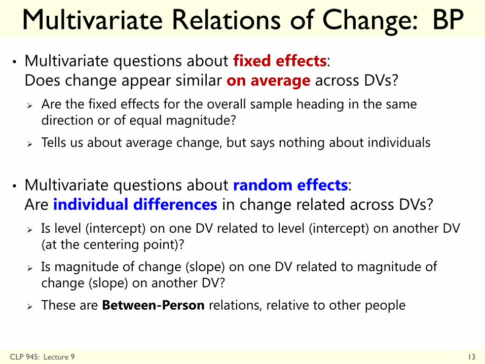
Multivariate Relations of Change: BP
• Multivariate questions about fixed effects:
Does change appear similar on average across DVs?
Are the fixed effects for the overall sample heading in the same
direction or of equal magnitude?
Tells us about average change, but says nothing about individuals
• Multivariate questions about random effects:
Are individual differences in change related across DVs?
Is level (intercept) on one DV related to level (intercept) on another DV
(at the centering point)?
Is magnitude of change (slope) on one DV related to magnitude of
change (slope) on another DV?
These are Between-Person relations, relative to other people
CLP 945: Lecture 9 13

Individual Relations of Functional and
Cognitive Change in Old Age
Functional Change Cognitive Change
CLP 945: Lecture 9 14

Individual Relations of Change in
Risky Behavior Across Siblings
Older Siblings Younger Siblings
CLP 945: Lecture 9 15
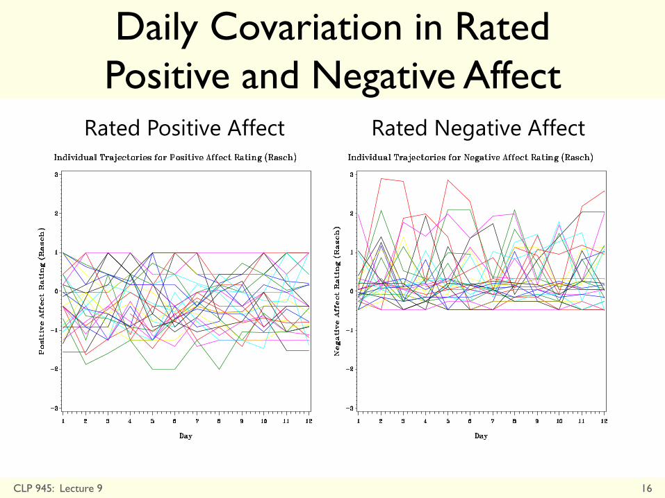
Daily Covariation in Rated
Positive and Negative Affect
Rated Positive Affect Rated Negative Affect
CLP 945: Lecture 9 16

Multivariate Model Level-2 G Matrix
Int DV A
Int DV B Slope DV A Slope DV B
Int DV A
Int DV B
Slope DV A
Slope DV B
0a
0b0a 0b
1a0a 1a0b 1a
1b0a 1b0b 1b1a 1b
2U
2U U
2U U U
2U U U U
τ
τ τ
τ τ τ
τ τ τ τ
G Matrix for Between-Person Random Effects Variances:
Estimate intercept and slope variances per DV and all covariances
DV = A
DV = B
Int-Int and
Slope-Slope
Covariances
CLP 945: Lecture 9 17
To estimate this model directly in univariate software, there will be no general
random intercept nor random “main” effects of predictors (i.e., as listed by
themselves). Instead, all random effects will be tied to a DV via an “interaction”
term (that actually creates nested versions of all fixed effects). Stay tuned…
Random Intercept Variances
Random Time
Slope Variances

Caveats about Correlated Random Effects
in Multivariate Longitudinal Models
• Random effects structure doesn’t have to match across DVs,
but it’s helpful if it does for their clearer interpretation
e.g., DV A has random intercept and slope, DV B has random intercept
only then random intercept is conditional on slope=0 only for DV A
• If random effects variances are small or nonsignificant,
covariances between them may not be estimated very well
Can always try it anyway if you do get some variance estimates
in the first place (i.e., numbers as opposed to dots)
Random effects solution may be unstable: numerically large correlations
may not be statistically significant due to large SEs for covariances
More DVs at once = more random effects harder to estimate
CLP 945: Lecture 9 18
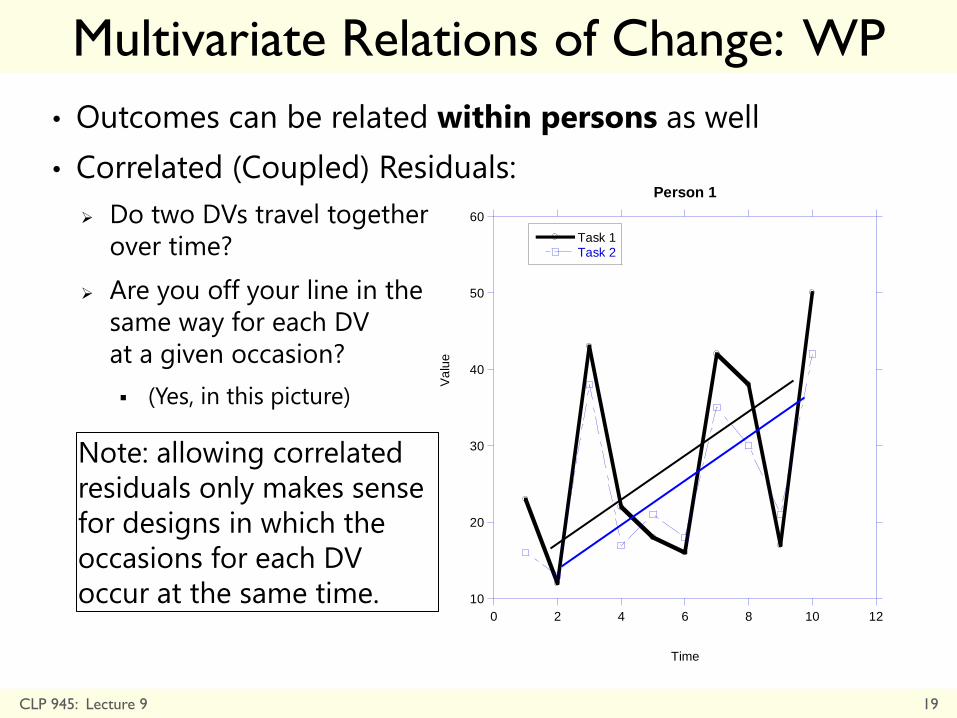
Multivariate Relations of Change: WP
10
20
30
40
50
60
0 2 4 6 8 10 12
Person 1
Task 1Task 2
Va
lue
Time
• Outcomes can be related within persons as well
• Correlated (Coupled) Residuals:
Do two DVs travel together
over time?
Are you off your line in the
same way for each DV
at a given occasion?
(Yes, in this picture)
Note: allowing correlated
residuals only makes sense
for designs in which the
occasions for each DV
occur at the same time.
CLP 945: Lecture 9 19

a
ab b
2e
2e e
Multivariate Model Level-1 R Matrix R Matrix for Within-Person Residual Variances: Estimate residual
variance per DV and covariance between DVs if at same occasion;
else estimate separate residual variances per DV without covariance
DV = A Residual Variance
DV = B Residual Variance
Res-Res Covariance: = covariance
remaining after accounting for any
individual effects of time
Res DV A Res DV B
Res DV A
Res DV B
CLP 945: Lecture 9 20
The categorical version of DV is used to structure the R matrix
as per occasion, per person. This assumes equal residual
variance with no covariance over time WITHIN EACH DV, but
residuals at the same occasion have a covariance across DVs.
Example SAS code:
REPEATED DV / R RCORR TYPE=UN SUBJECT=Wave*Person

What about Multivariate Alternative
Covariance Structures Models? • We will examine multivariate random effects models. Are there
multivariate versions of alternative covariance structures?
• Yes, but they are much more limited—3 real options in SAS:
Direct product structures: TYPE= UN@UN, UN@AR1
Assumes equal variances across time
Assumes same pattern of autocorrelation holds for each DV!
See REPEATED statement in SAS manual for further explanation
Completely unstructured multivariate
Specify DV*occasion on REPEATED statement
Estimates all possible variances and covariances separately, so it will fit the best, but with the least parsimony in doing so
No random effects = no between- and within-person separation
Just specify a random intercept (i.e., assume compound symmetry)
Not optimal, but it’s the best I can come up with (for now)
CLP 945: Lecture 9 21

Multivariate Multilevel Models
for Longitudinal Data
(as in SAS and Mplus)
CLP 945: Lecture 9 22
• Topics:
Univariate vs. multivariate approaches for modeling
time-varying (or any lower-level) predictors
Multivariate relations of change (per level of analysis)
Multivariate tests of differences in effect size and
their specification in univariate MLM software
What not to do: smushed effects path models
for longitudinal data
Single-level SEM for multivariate multilevel models
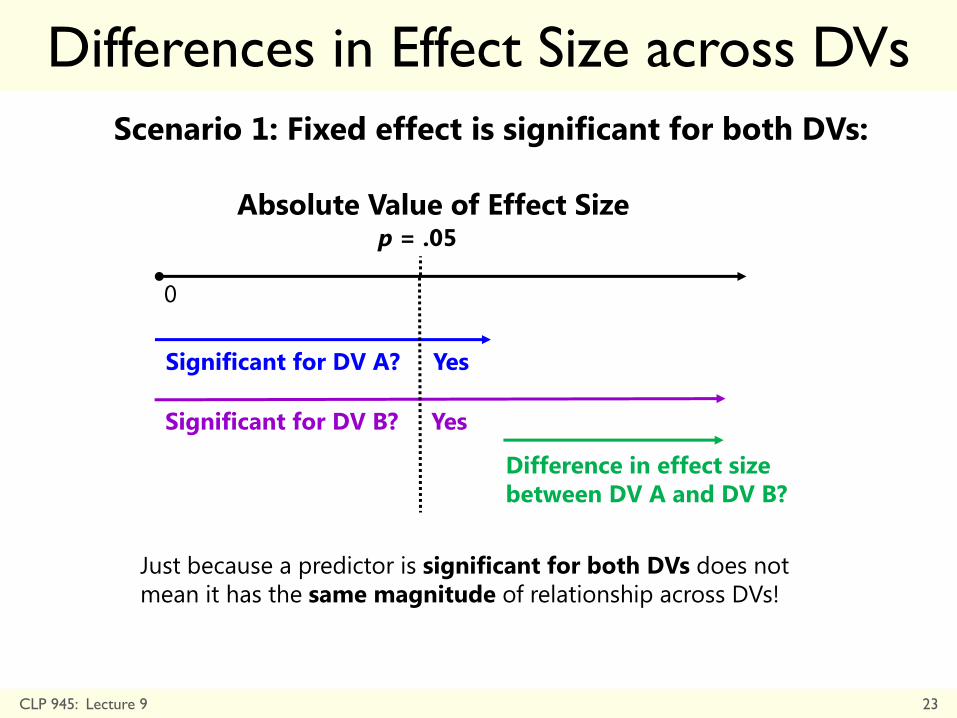
Differences in Effect Size across DVs
Absolute Value of Effect Size
0
p = .05
Significant for DV A? Yes
Significant for DV B? Yes
Difference in effect size
between DV A and DV B?
Scenario 1: Fixed effect is significant for both DVs:
Just because a predictor is significant for both DVs does not
mean it has the same magnitude of relationship across DVs!
CLP 945: Lecture 9 23

Differences in Effect Size across DVs
Absolute Value of Effect Size
0
Significant for DV A? No
Significant for DV B? Yes
Difference in effect size
between DV A and DV B?
Scenario 1: Fixed effect is significant for DV B only:
p = .05
Also, just because a predictor is non-significant for one DV
but significant for another DV does not mean it has
different magnitudes of relationships across DVs!
CLP 945: Lecture 9 24

Why multivariate models should be
used to test differences in effect sizes:
• Testing differences in effect size of predictors requires all DVs in
the same model!
• But if the effects are the same, you can specify a single effect across
DVs to reduce the number of estimated parameters.
• Hypotheses about difference scores are best tested using the
original outcomes that created the difference in a multivariate
model so that information about absolute amount is also provided.
• If DVs have missing data but are correlated, then tests of fixed
effects may have more power in a multivariate model.
• Keep in mind that these models test differences in unstandardized
fixed effects, so the DVs need to be on the same scale (or should be
transformed onto the same scale before-hand otherwise).
CLP 945: Lecture 9 25

Tricking Univariate MLM Software into
Estimating Multivariate MLMs (here, 2 DVs) Outcome DV dvA dvB Wave
Yi1a A 1 0 1
Yi2a A 1 0 2
Yi3a A 1 0 3
Yi4a A 1 0 4
Yi5a A 1 0 5
Yi6a A 1 0 6
Yi1b B 0 1 1
Yi2b B 0 1 2
Yi3b B 0 1 3
Yi4b B 0 1 4
Yi5b B 0 1 5
Yi6b B 0 1 6
1. Double-stack all DVs
into a single outcome
2. Create a categorical
predictor for which DV
is which (e.g., A,B)
3. Create a dummy
variable for each
dvA= (1,0)
dvB= (0,1)
4. Keep all other
variables
This shows data for 1 person,
2 outcomes, over 6 waves.
We’ll use “DV” to structure the G and R
matrices, and “dvA” and “dvB” to create DV-
specific fixed effects in the model for the means.
CLP 945: Lecture 9 26

“Direct Effects” Multivariate Model Within-Person Level 1: t = Time crossed with d = DV
ytid = dvA[β0ia + β1ia(Timetia) + etia]
dvB[β0ib + β1ib(Timetib) + etib]
Between-Person Level 2: i = individual crossed with d = DV
β0ia = γ00a + γ01a(Predi) + U0ia
β1ia = γ10a + γ11a(Predi) + U1ia
β0ib = γ00b + γ01b(Predi) + U0ib
β1ib = γ10b + γ11b(Predi) + U1ib
CLP 945: Lecture 9 27
If DV=A, the βia are awake
If DV=B, the βib are awake
Intercept and time
slope for DV=A
Intercept and time
slope for DV=B
To estimate this model directly in univariate software, there will be no general
fixed intercept (via option NOINT) nor “main” effects of predictors (i.e., as listed
by themselves). Instead, all fixed effects will be tied to a DV via an “interaction”
term (that actually creates nested versions of all fixed effects). Let’s see how…

Multivariate MLM in Univariate MLM
Software: “Direct Effects” Version * "Outcome" variable holds both DV A and DV B in one column;
* IMPORTANT: NOINT is needed to shut off general intercept,
so that dvA and dvB become the intercepts per DV;
PROC MIXED DATA=work.multivstacked COVTEST NOCLPRINT NAMELEN=100 IC METHOD=REML;
* Level-2 ID, Level-1 ID, DV ID;
CLASS PersonID Wave DV;
* This version lists all fixed and random effects being estimated,
where the dv interactions specify each effect per DV;
MODEL outcome = dvA dvB dvA*time dvB*time dvA*pred dvB*pred
dvA*time*pred dvB*time*pred / NOINT DDFM=Satterthwaite;
RANDOM dvA dvB dvA*time dvB*time / G GCORR TYPE=UN SUBJECT=PersonID;
* This version does the exact same thing with less code;
MODEL outcome = DV DV*time DV*pred DV*time*pred / NOINT DDFM=Satterthwaite;
RANDOM DV DV*time / G GCORR TYPE=UN SUBJECT=PersonID;
* This line adds separate residual variances per DV and covariance;
REPEATED DV / R RCORR TYPE=UN SUBJECT=PersonID*Wave;
* If you do not want a residual covariance, do this instead, which
still allows separate residual variances per DV via first diagonal;
REPEATED DV / R RCORR TYPE=TOEPH(1) SUBJECT=PersonID*Wave;
CLP 945: Lecture 9 28

Multivariate MLM in Univariate MLM
Software: “Direct Effects” Version
• Pros of previous “direct effects” version of model:
Fixed effects solution gives significance test for every effect per DV
Type 3 Tests (multivariate Wald tests automatic in SAS and SPSS)
gives significance test for each effect combined across DVs
Is easier to do correctly, particularly if not all effects are included per DV
MODEL outcome = dvA dvB dvA*pred says no effect of pred for dv B
• Cons of “direct effects” version of model:
Does NOT give you tests of differences in effects across DVs, so you will
need to write ESTIMATE or CONTRAST statements to obtain those
• To get the significance of the differences in effects across DVs
automatically, switch to the “differences in effects” version
But then you only get significance of fixed effects for the reference DV
CLP 945: Lecture 9 29

Multivariate MLM in Univariate MLM
Software: “Difference in Effects” Version * Everything else is the same (PROC MIXED, CLASS, REPEATED), but
the removal of NOINT changes the interpretation of what DV does;
* NOW the effect of DV indicates the difference between DVs (relative to a
reference DV, highest numerically or last alphabetically) in each effect;
MODEL outcome = DV time DV*time pred DV*pred
time*pred DV*time*pred / DDFM=Satterthwaite;
Type 3 Tests (multivariate Wald tests automatic in SAS and SPSS) will now give combined significance test differences in effects across all DVs
* You can still use the direct effects version for random effects if you want;
RANDOM DV DV*time / G GCORR TYPE=UN SUBJECT=PersonID;
* Or this version gives you the difference between DVs as random effects,
which may be harder to estimate in some cases than the direct effects version;
RANDOM INTERCEPT DV time DV*time / G GCORR TYPE=UN SUBJECT=PersonID;
CLP 945: Lecture 9 30

Summary: Multivariate MLMs permit… • Tests of hypotheses about BP relations (among intercepts and
slopes) and WP relations (among time-specific residuals)
BP: Does intercept on one DV correlate with level on another DV?
BP: Does change on one DV correlate with change on another DV?
WP: Do two DVs ‘travel together’ over time within persons?
Questions involving directed relationships among DVs instead require “truly” multivariate MLM software instead of tricking univariate MLM software (which can only phrase these relationships as covariances in L2 G and L1 R)
• Tests about differences in effect size of predictors across DVs
Is the effect of the predictor significant per DV?
Is the effect of the predictor significantly different across DVs?
These questions can be answered in any kind of MLM software
• Multivariate multilevel models (or “Multilevel-SEM”) can usually be phrased similarly using measurement models for latent variables within a single-level SEM framework… we’ll see how this works.
CLP 945: Lecture 9 31

Multivariate Multilevel Models
for Longitudinal Data
(in SAS and Mplus)
CLP 945: Lecture 9 32
• Topics:
Univariate vs. multivariate approaches for modeling
time-varying (or any lower-level) predictors
Multivariate relations of change (per level of analysis)
Multivariate tests of differences in effect size and
their specification in univariate MLM software
What not to do: smushed effects path models
for longitudinal data
Single-level SEM for multivariate multilevel models

What Not to Do with Longitudinal Data
• Mis-specified path models (involving observed variables only)
for longitudinal data are still far too common
These models include auto-regressive effects, cross-lagged effects, and
observed variable mediation models involving different variables each
measured on two or more occasions
Common exemplars to watch out for are given on the next slides
• The problem in each is a lack of differentiation of sources
(piles) of variance, and thus what their effects mean
If the path model variables have not been de-trended for person mean
differences (and for any individual change over time), then all estimated
paths will be smushed BP/WP to some degree
CLP 945: Lecture 9 33

A Model that Needs to Die*
• Logic: by including auto-regressive paths (B1 and B2) to “control” for previous occasions, the cross-lagged paths (B3 and B4) then represent effects of “change” on each variable in predicting the other (so they are “longitudinal” predictions)
• Reality: by allowing only one path, it smushes effects across sources of variance—BP intercept, BP slope(s), WP residual; autoregressive paths between occasions do NOT control for BP differences (assumes an AR(1) correlation model over time)
CLP 945: Lecture 9 34
Autoregressive
cross-legged
panel model
* Emphasis mine, logic
and picture provided by
Berry & Willoughby (2017,
Child Development)

And take this one with it*…
• Logic: mediation should time to occur, so indirect effects
should be specified across occasions (as before, of “change”)
• Agreed, but if these variables haven’t been de-trended for all
sources of BP variance, then the b and c paths are smushed
• And what about BP mediation? Capturing BP variances in the
same model would allow examination of that, too, right?
CLP 945: Lecture 9 35
Longitudinal
mediation model X= IV, M= mediator, Y= DV
* My point of view only, picture
provided by Maxwell & Cole
(2007, Psychological Methods)

How to Fix It: Translating MLM’s Variance
Partitioning into Single-Level SEM
• “Random effects” = “pile of variance’’ = “variance components”
Random effects represent person*something interaction terms that create person-caused sources of covariance over time
Random intercept person*intercept (person “main effect”)
Random linear time slope person*time interaction
• Random effects are the same thing as latent variables
Latent variable = unobservable ability or trait, created by sources of common variance across items (or time-specific outcomes here)
Latent variables for BP differences can be interpreted as “general tendency” (random intercept) and “propensity to change” (random time slope)
Model-based way of de-trending longitudinal outcomes to distinguish BP from WP sources of information (and examine all kinds of relations)
Uses “wide” data structure in which each occasion = separate variable
CLP 945: Lecture 9 36

MLM as seen through
Confirmatory Factor Analysis (CFA) • CFA model: yis = μi + λiFs + eis (SEM is just relations among F’s)
Observed response for item i ( outcome at time t) and subject s
= intercept of item i (μ)
+ subject s’s latent trait/factor (F), item-weighted by λ
+ error (e) of item i and subject s
• Four big differences when using CFA/SEM for longitudinal change:
Usually two factors for “level” and “change” (intercept and slope):
yti = (γ00 + U0i) + (γ10 + U1i)timeti + eti so the U’s are the F’s
The separate item (time-specific outcome) intercepts μi cannot be identified from
the “intercept” factor and therefore must be fixed to 0
The factor loadings λi for how each outcome is predicted by the latent factor are
usually pre-determined by how much time as passed, and are fixed to the difference
in time that corresponds to the type of change (e.g., linear, quadratic, piecewise)
Item (time-specific outcome) residual variances should be constrained equal (not
default, but changes in variance over time should be captured by random slopes)
CLP 945: Lecture 9 37

Random Effects as Latent Variables
• BP model: eti-only model for the variance
yti = γ00 + eti
After controlling for the fixed intercept, residuals are
assumed uncorrelated: this is a single-level model
Int
Y1 Y2 Y3 Y4
e1 e2 e3 e4
1 1 1 1
Int Var
𝛕𝐔𝟎𝟐 = 𝟎
Mean of the intercept factor
= fixed intercept γ00
Loadings of intercept factor = 1
(all occasions contribute equally)
Item intercepts = 0 (always)
Variance of intercept factor
= 0 so far
Residual variance (e) is assumed to
be equal across occasions = = =
CLP 945: Lecture 9 38

Random Effects as Latent Variables
• +WP model: U0i + eti model for the variance
yti = γ00 + U0i + eti
After controlling for the random intercept, residuals are
assumed uncorrelated: now two piles of variance (what we
would call an “empty means, random intercept model)
CLP 945: Lecture 9 39
Int
Y1 Y2 Y3 Y4
e1 e2 e3 e4
1 1 1 1
Int Var
𝛕𝐔𝟎𝟐 =?
Mean of the intercept factor
= fixed intercept γ00
Loadings of intercept factor= 1
(all occasions contribute equally)
Variance of intercept factor
= random intercept variance
Residual variance (e) is assumed to
be equal across occasions
= = =

Random Effects as Latent Variables
• Fixed linear time, random intercept model:
yti = γ00 + (γ10Timeti) + U0i + eti
After controlling for the fixed linear slope and random
intercept, residuals are assumed uncorrelated
CLP 945: Lecture 9 40
Int
Y1 Y2 Y3 Y4
e1 e2 e3 e4
1 1 1
1
Int Var
𝛕𝐔𝟎𝟐 =?
Mean of the linear slope factor
= fixed linear slope γ10
Loadings of linear slope factor
= occasions (keep real time)
Variance of linear slope factor
= 0
Linear
Slope 0 1
2 3
Linear
Slope Var
𝛕𝐔𝟏𝟐 =0
= = =

Random Effects as Latent Variables
• Random linear model:
yti = γ00 + (γ10Timeti) + U0i + (U1iTimeti) + eti
After controlling for the random linear slope and random
intercept, residuals are assumed uncorrelated: now three
piles of variance to be predicted (BP int, BP slope, WP res)
CLP 945: Lecture 9 41
Int
Y1 Y2 Y3 Y4
e1 e2 e3 e4
1 1 1
1
Int Var
𝛕𝐔𝟎𝟐 =?
Mean of the linear slope factor
= fixed linear slope γ10
Loadings of linear slope factor
= occasions (keep real time)
Variance of linear slope factor
= random slope variance (and
covariance with random intercept
Linear
Slope 0 1
2 3
Linear
Slope Var
𝛕𝐔𝟏𝟐 =?
= = =
τU01

Adding Level-2 Predictors
Level 1: yti = β0i + β1i(Timeti) + eti
Level-2: β0i = γ00 + γ01(Groupi) + U0i
β1i = γ10 + γ11(Groupi) + U1i
CLP 945: Lecture 9 42
Int
Y1 Y2 Y3 Y4
e1 e2 e3 e4
1 1 1
1
Int Var
𝛕𝐔𝟎𝟐 =?
Linear
Slope 0 1
2 3
Linear
Slope Var
𝛕𝐔𝟏𝟐 =?
= = =
τU01
Group γ01
γ11 Mean of the intercept factor
= fixed intercept γ00
Mean of the linear slope factor
= fixed linear slope γ10
Loadings of linear slope factor
= occasions (keep real time)
Variance of linear slope factor
= random slope variance

yti = γ00 + (γ10Timeti) + U0i + (U1iTimeti) + eti
Summary: Random Linear Time Model
as Latent Variables in SEM
CLP 945: Lecture 9 43
Int
Y1 Y2 Y3 Y4
e1 e2 e3 e4
1 1 1
1
Int Var
𝛕𝐔𝟎𝟐 =?
Linear
Slope 0 1
2 3
Linear
Slope Var
𝛕𝐔𝟏𝟐 =?
= = =
Level-1 R Matrix
Level-1
Z Matrix
𝛕𝐔𝟎𝟏= ?
Level-2 G Matrix
MLM matrix version of model
Overall:
Model for the Variance:
i i i i i = + Y X γ Z U E
Ti i i i i V Z G Z R

Multivariate MLM as Single-Level SEM
This diagram is from the Mplus
v. 8 Users Guide example 6.13.
The two-headed arrows
between the intercept factors
(i1 and i2) and between the
slope factors (s1 and s2) convey
undirected covariances.
The single-headed arrows from
i1 to s2 and from i2 to s1 are
directed regressions which
convey directionality (although
this model fits equivalently
whether one uses directed
regressions or covariances
among the latent factors).
CLP 945: Lecture 9 44

Summary: Random Effects Phrased as
Latent Variables in Single-Level SEM • Random effects are person-specific sources of covariation among
outcomes over time—these are the same as latent variables
Time-specific outcomes become “items” in factor analysis
Factor loadings convey time span and pattern of change
You can use individually varying time loadings for unbalanced data—via TSCORES in Mplus—which means absolute fit assessment is not provided
Fixed effect = latent variable mean (“mean” “intercept” if predicted)
Random effect variance = latent variable variance (“variance” “residual” variance if predicted)
Covariances among random effects in multivariate MLM can also be phrased as directed regressions (in “truly” multivariate MLM, M-SEM, or SEM)
• For univariate or multivariate longitudinal models with only level-2 predictors, MLM single-level SEM with no real problem
This is NOT true for time-varying predictors, the specification of which are still frequently misunderstood in single-level SEMs
CLP 945: Lecture 9 45

Time-Varying Predictors in Single-Level
SEM: What Not to Do
CLP 945: Lecture 9 46
This diagram is from the Mplus
v. 8 Users Guide example 6.10.
Although the y11-y14
outcomes are predicted by
latent intercept and slope
factors (separating two kinds
of BP variance from WP
variance), this is not the case
for the a31-a34 outcomes.
Consequently, in the model
shown here, the ay paths will
be smushed effects.
Time-Varying Predictors in Single-Level
SEM: What Not to Do (continued)
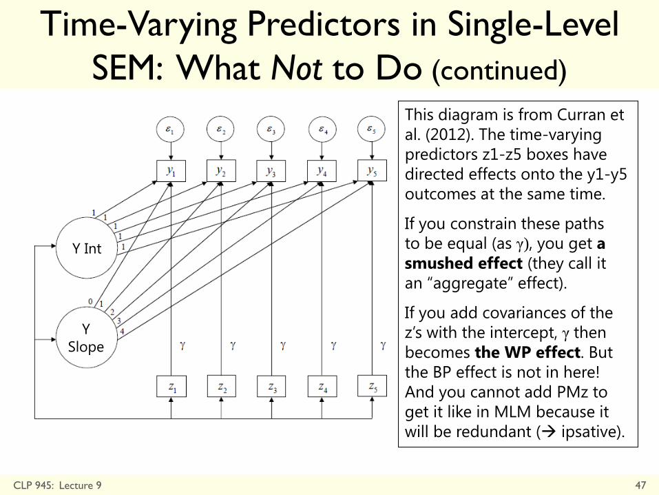
This diagram is from Curran et
al. (2012). The time-varying
predictors z1-z5 boxes have
directed effects onto the y1-y5
outcomes at the same time.
If you constrain these paths
to be equal (as γ), you get a
smushed effect (they call it
an “aggregate” effect).
If you add covariances of the
z’s with the intercept, γ then
becomes the WP effect. But
the BP effect is not in here!
And you cannot add PMz to
get it like in MLM because it
will be redundant ( ipsative).
Y Int
Y
Slope
CLP 945: Lecture 9 47

How to Fix It (by Curran et al., 2012)
CLP 945: Lecture 9 48
The z1-z5 time-varying
predictors now have their own
intercept factor, which directly
represents their BP intercept
variance.
So the BP intercept effect is
given by γα, and the WP
effect is now given by γ from
the residuals of z1-z5 y1-y5.
Y Int
Y
Slope
Z Int
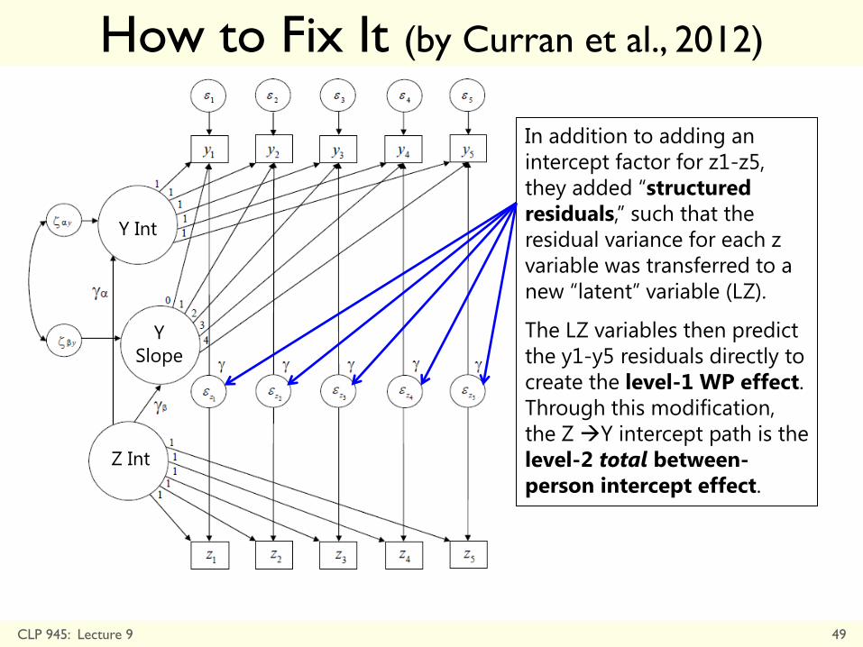
How to Fix It (by Curran et al., 2012)
CLP 945: Lecture 9 49
In addition to adding an
intercept factor for z1-z5,
they added “structured
residuals,” such that the
residual variance for each z
variable was transferred to a
new “latent” variable (LZ).
The LZ variables then predict
the y1-y5 residuals directly to
create the level-1 WP effect.
Through this modification,
the Z Y intercept path is the
level-2 total between-
person intercept effect.
Y Int
Y
Slope
Z Int

Another Example of Structured Residuals
If z1-z5 has individual differences in change over time instead of just fluctuation, just add a slope factor for z1-z5—then you’d be back to multivariate multilevel model we began with.
When using level-1 structured residuals, all paths among the intercept and slope factors will represent their total level-2 BP effects.
CLP 945: Lecture 9 50
From Curran et al. (2014; Journal of
Consulting and Clinical Psychology)

How To Fix It Without Structured Residuals
CLP 945: Lecture 9 51
IF you predict the y1-y5
residuals directly from z1-z5
(without structured residuals),
that effect is still the level-1
WP effect.
The problem (in Mplus) is that
some of the paths among the
intercept and slope factors
become BP contextual effects
instead. These include paths for
intercept intercept and slope
slope, but not for intercept
slope (or slope intercept).
In either version, you can still
get the missing L2 effect (BP
total or BP contextual) by
requesting a NEW effect in
MODEL CONSTRAINT.

When to Use Each:
Multivariate MLM vs Single-Level SEM • Models and software are logically separate, but (current)
software restrictions may make it so one version is easier than the other for specifying certain types of models
• “Truly” Multivariate MLM (e.g., MLM side of Mplus):
Uses stacked data, so *contemporaneous* level-1 is explicit, which easily allows for random effects of level-1 predictors, mediation, and/or measurement models at each level of analysis
However: be careful of otherwise equivalent Mplus models whose L2 parameters change interpretation with different version of the syntax!
• Single-Level SEM (e.g., SEM side of Mplus):
Uses wide data structure, so level-1 parameters must be specified through constraints across multiple observed variables, which assumes balanced time (Mplus Tscores that allows individually varying times for growth models is not relevant for WP fluctuation models)
CLP 945: Lecture 9 52

When to Use Each:
Multivariate MLM vs Single-Level SEM • Models requiring access to level-1 observations at different
occasions across DVs can be easier to do in single-level SEM
• Single-Level SEM (e.g., SEM side of Mplus):
All occasions are accessible at once, which means that patterns of residual covariance over time can be easily included (via constraints)
Lagged residual relationships across DVs can be easily included (e.g., time 1 X time 2 Y, time 1 Y time 2 X), just make sure to not smush!
• Multivariate MLM (e.g., MLM side of Mplus):
Uses stacked data, so it doesn’t have access to previous occasions’ information stored on different rows (which needs to be unsmushed)
Mplus 8 allows auto-regressive relations, but only as specified as directed paths (not residual covariances) and only by using Bayes MCMC estimation
CLP 945: Lecture 9 53

Summary:
Multivariate Longitudinal Modeling • Models and software are logically separate
No single approach/program can do everything you want; software options will always vary in what is possible and in how conveniently each model can be specified
• Univariate MLM:
Easy to specify in many widely available software packages; has REML estimation
Limited to multivariate multilevel models whose outcome relations can be phrased as covariances (in L2 G or L1 R), not directed paths (as needed in mediation)
• “Truly” Multivariate MLM (or M-SEM):
Trickier to specify correctly; available in many fewer (expensive) packages
More flexible for adding levels of analysis or specifying level-specific associations
• Single-Level SEM:
Harder to phrase level-specific associations, largely built for balanced data
Easier to specify relations across different occasions as variables than as rows of data
CLP 945: Lecture 9 54