Embed Size (px)
Citation preview
MULTITASKING AND SCHEDULING
EEN 417Fall 2013
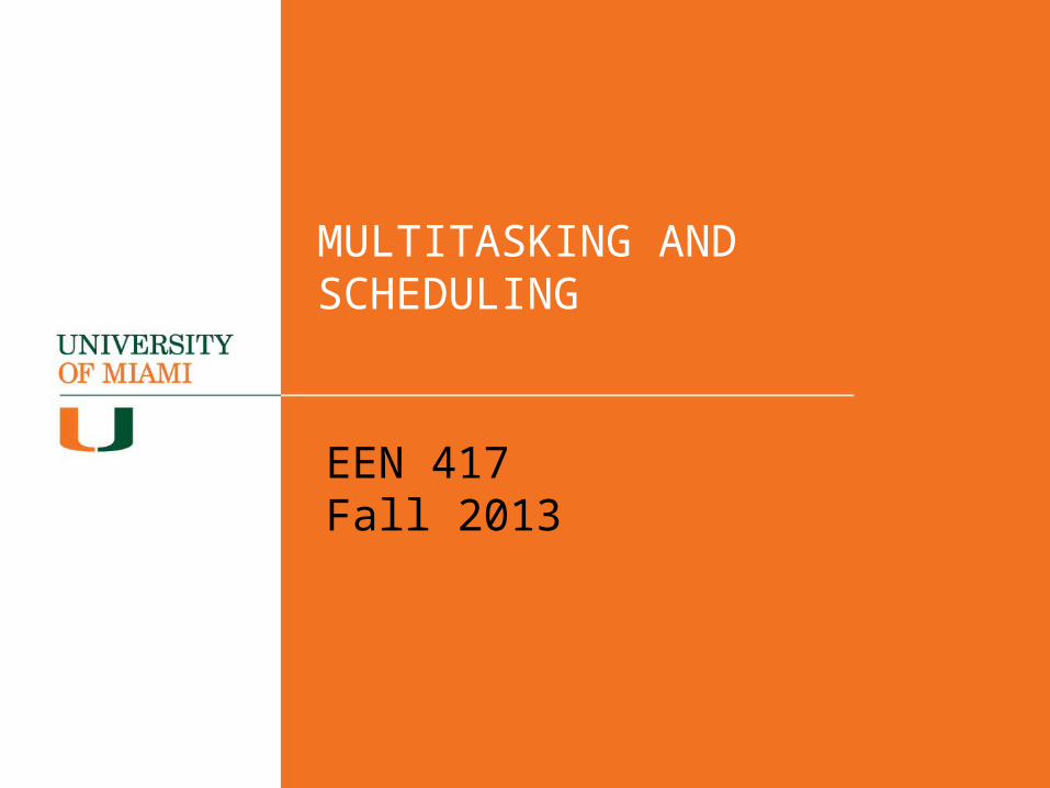
Layers of Abstraction for Concurrency in Programs
What is a thread?
• Definition?
Definition and Uses• Threads are sequential procedures that share memory.
• Uses of concurrency: Reacting to external events (interrupts) Exception handling (software interrupts) Creating the illusion of simultaneously running different programs (multitasking) Exploiting parallelism in the hardware (e.g. multicore machines). Dealing with real-time constraints.
Thread Scheduling• Predicting the thread schedule is an iffy proposition.
Without an OS, multithreading is achieved with interrupts. Timing is determined by external events.
Generic OSs (Linux, Windows, OSX, …) provide thread libraries (like “pthreads”) and provide no fixed guarantees about when threads will execute.
Real-time operating systems (RTOSs), like QNX, VxWorks, RTLinux, Windows CE, support a variety of ways of controlling when threads execute (priorities, preemption policies, deadlines, …).
Processes vs. Threads?
Processes vs. Threads?
Processes are collections of threads with their own memory, not visible to other processes. Segmentation faults are attempts to access memory not allocated to the process. Communication between processes must occur via OS facilities (like pipes or files).
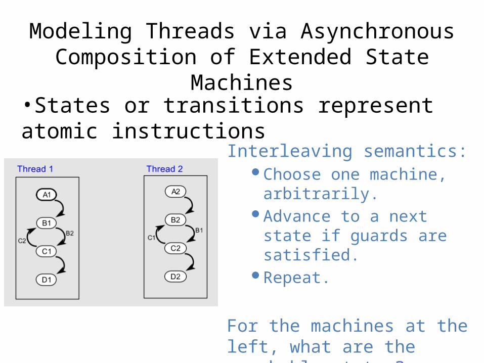
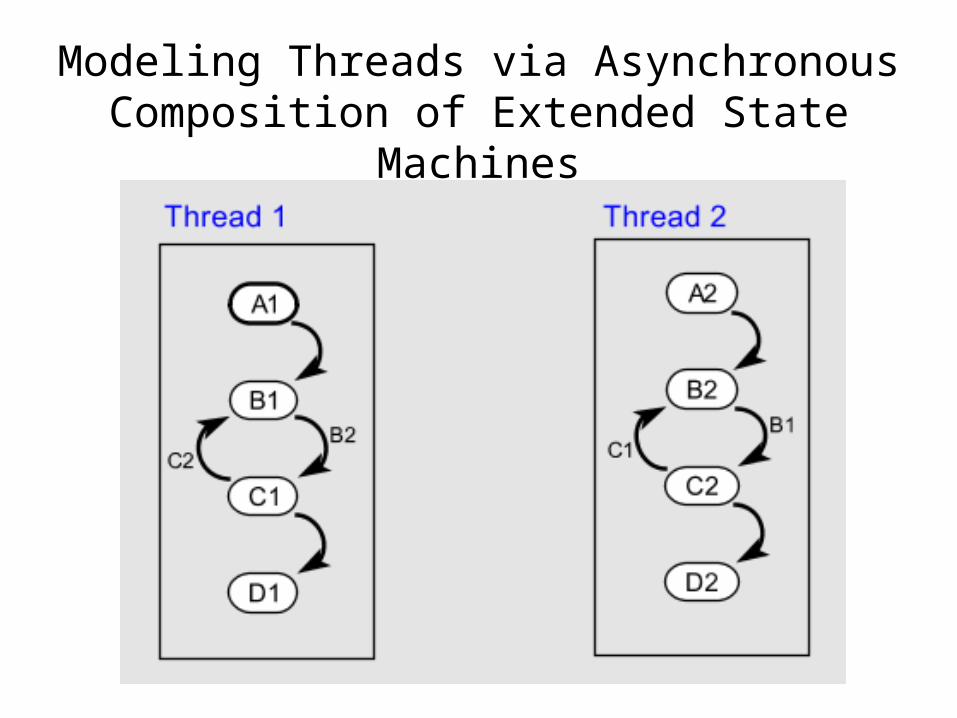
Modeling Threads via Asynchronous Composition of Extended State Machines
•States or transitions represent atomic instructions
Interleaving semantics:Choose one machine,
arbitrarily.Advance to a next state if
guards are satisfied.Repeat.
For the machines at the left, what are the reachable states?
Modeling Threads via Asynchronous Composition of Extended State Machines
This is a very simple, commonly used design pattern. Perhaps Concurrency is Just Hard…
•Sutter and Larus observe:
•“humans are quickly overwhelmed by concurrency and find it much more difficult to reason about concurrent than sequential code. Even careful people miss possible interleavings among even simple collections of partially ordered operations.”
•H. Sutter and J. Larus. Software and the concurrency revolution. ACM Queue, 3(7), 2005.
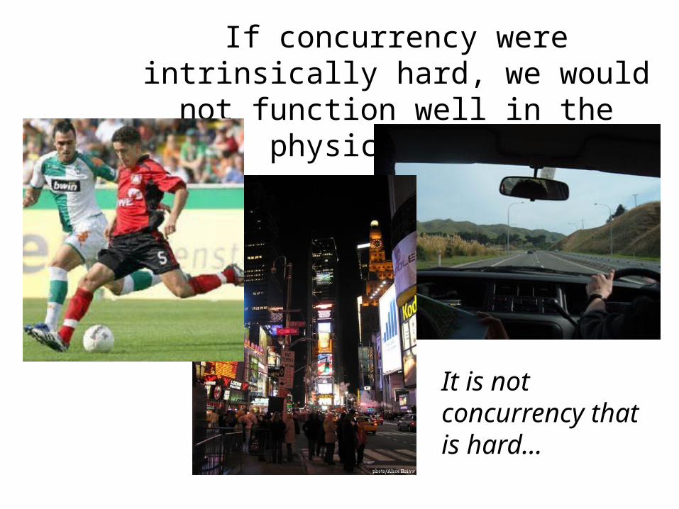
If concurrency were intrinsically hard, we would not function well in the physical
world
It is not concurrency that is hard…
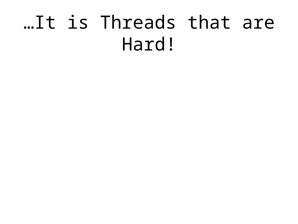
…It is Threads that are Hard!•Threads are sequential processes that share memory. From the perspective of any thread, the entire state of the universe can change between any two atomic actions (itself an ill-defined concept).
•Imagine if the physical world did that…
Problems with the Foundations•A model of computation:
• Bits: B = {0, 1}• Set of finite sequences of bits: B*
• Computation: f : B* B*
• Composition of computations: f f '• Programs specify compositions of computations
•Threads augment this model to admit concurrency.
•But this model does not admit concurrency gracefully.
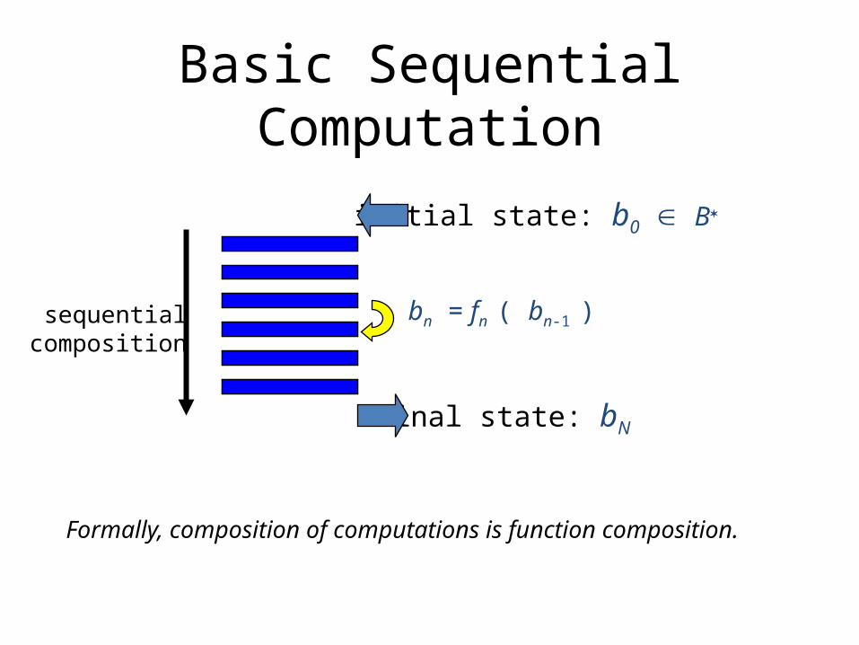
Basic Sequential Computation
initial state: b0 B*
final state: bN
sequentialcomposition
bn = fn ( bn-1 )
Formally, composition of computations is function composition.
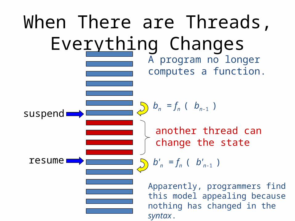
When There are Threads,Everything Changes
suspend
A program no longer computes a function.
resume
another thread can change the state
bn = fn ( bn-1 )
b'n = fn ( b'n-1 )
Apparently, programmers find this model appealing because nothing has changed in the syntax.
Succinct Problem Statement•Threads are wildly nondeterministic.
•The programmer’s job is to prune away the nondeterminism by imposing constraints on execution order (e.g., mutexes) and limiting shared data accesses (e.g., OO design).
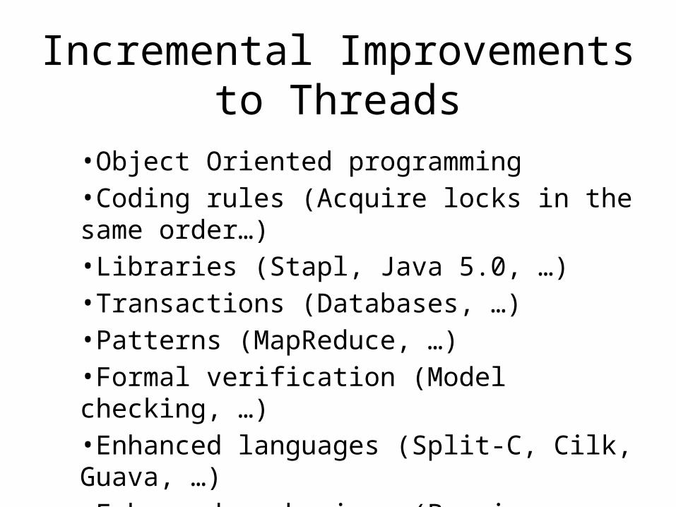
Incremental Improvements to Threads
•Object Oriented programming •Coding rules (Acquire locks in the same order…)•Libraries (Stapl, Java 5.0, …)•Transactions (Databases, …)•Patterns (MapReduce, …)•Formal verification (Model checking, …)•Enhanced languages (Split-C, Cilk, Guava, …)•Enhanced mechanisms (Promises, futures, …)
SCHEDULING
Responsibilities of a Microkernel(a small, custom OS)
Scheduling of threads or processes– Creation and termination of threads– Timing of thread activations
Synchronization– Semaphores and locks
Input and output– Interrupt handling
A Few More Advanced Functions of an Operating System – Not discussed here…
Memory management– Separate stacks– Segmentation– Allocation and deallocation
File system– Persistent storage
Networking– TCP/IP stack
Security– User vs. kernel space– Identity management
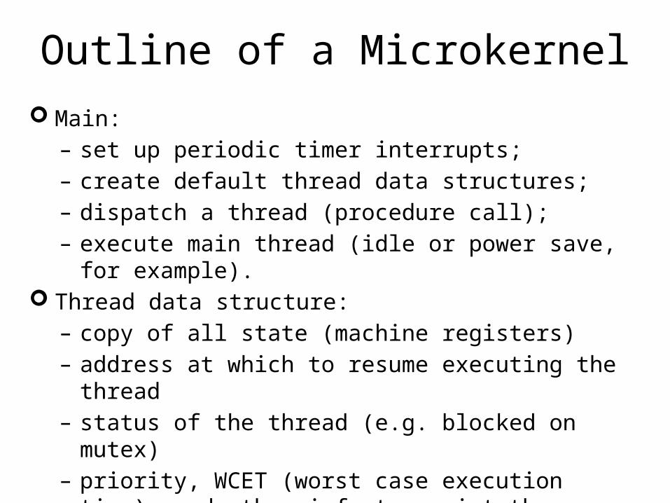
Outline of a Microkernel
Main:– set up periodic timer interrupts;– create default thread data structures;– dispatch a thread (procedure call);– execute main thread (idle or power save, for example).
Thread data structure:– copy of all state (machine registers)– address at which to resume executing the thread– status of the thread (e.g. blocked on mutex)– priority, WCET (worst case execution time), and other
info to assist the scheduler
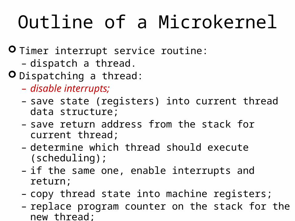
Outline of a Microkernel Timer interrupt service routine:
– dispatch a thread. Dispatching a thread:
– disable interrupts;– save state (registers) into current thread data structure;– save return address from the stack for current thread;– determine which thread should execute (scheduling);– if the same one, enable interrupts and return;– copy thread state into machine registers;– replace program counter on the stack for the new thread;– enable interrupts;– return.
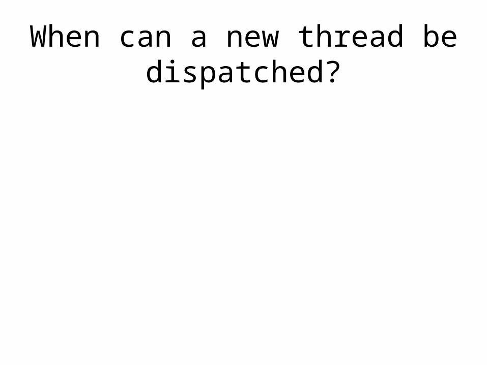
When can a new thread be dispatched?
Under non-preemptive scheduling:– When the current thread completes.
Under Preemptive scheduling:– Upon a timer interrupt– Upon an I/O interrupt (possibly)– When a new thread is created, or one completes.– When the current thread blocks on or releases a mutex– When the current thread blocks on a semaphore– When a semaphore state is changed– When the current thread makes any OS call
• file system access• network access• …
The Focus Today:How to decide which thread to schedule?
• Considerations:Preemptive vs. non-preemptive schedulingPeriodic vs. aperiodic tasksFixed priority vs. dynamic priorityPriority inversion anomaliesOther scheduling anomalies
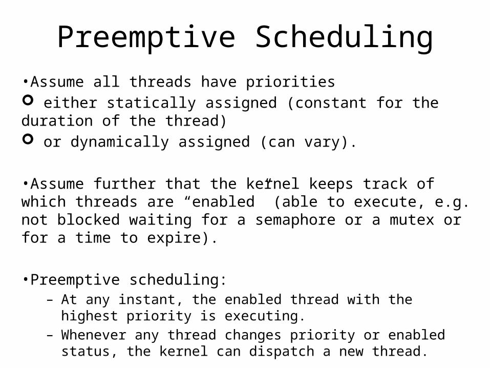
Preemptive Scheduling•Assume all threads have priorities either statically assigned (constant for the duration of the thread) or dynamically assigned (can vary).
•Assume further that the kernel keeps track of which threads are “enabled” (able to execute, e.g. not blocked waiting for a semaphore or a mutex or for a time to expire).
•Preemptive scheduling:– At any instant, the enabled thread with the highest priority is
executing.– Whenever any thread changes priority or enabled status, the kernel
can dispatch a new thread.
Rate Monotonic Scheduling•Assume n tasks invoked periodically with:
– periods T1, … ,Tn (impose real-time constraints)
– worst-case execution times (WCET) C1, … ,Cn • assumes no mutexes, semaphores, or blocking I/O
– no precedence constraints– fixed priorities– preemptive scheduling
•Theorem: If any priority assignment yields a feasible schedule, then priorities ordered by period (smallest period has the highest priority) also yields a feasible schedule.•RMS is optimal in the sense of feasibility.
Liu and Leland, “Scheduling algorithms for multiprogramming in a hard-real-time environment,” J. ACM, 20(1), 1973.
Feasibility for RMS•Feasibility is defined for RMS to mean that every task executes to completion once within its designated period.
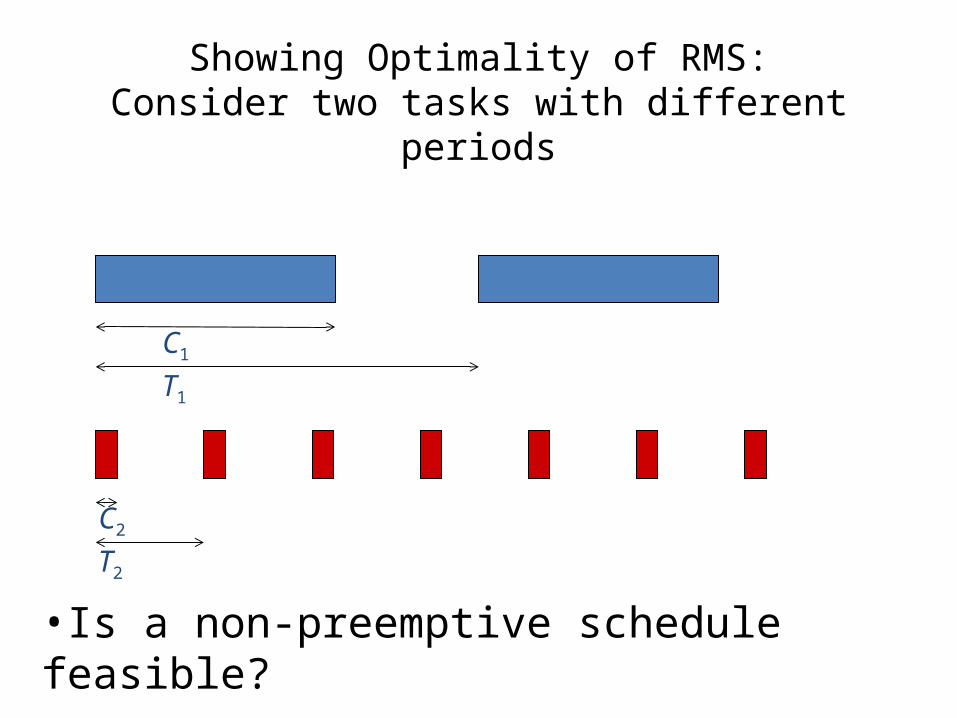
Showing Optimality of RMS:Consider two tasks with different periods
•Is a non-preemptive schedule feasible?
C1
T1
C2
T2
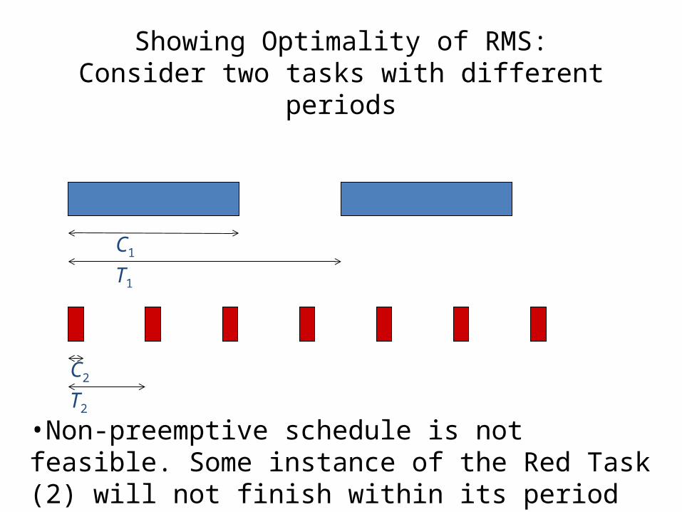
Showing Optimality of RMS:Consider two tasks with different periods
•Non-preemptive schedule is not feasible. Some instance of the Red Task (2) will not finish within its period if we do non-preemptive scheduling.
C1
T1
C2
T2
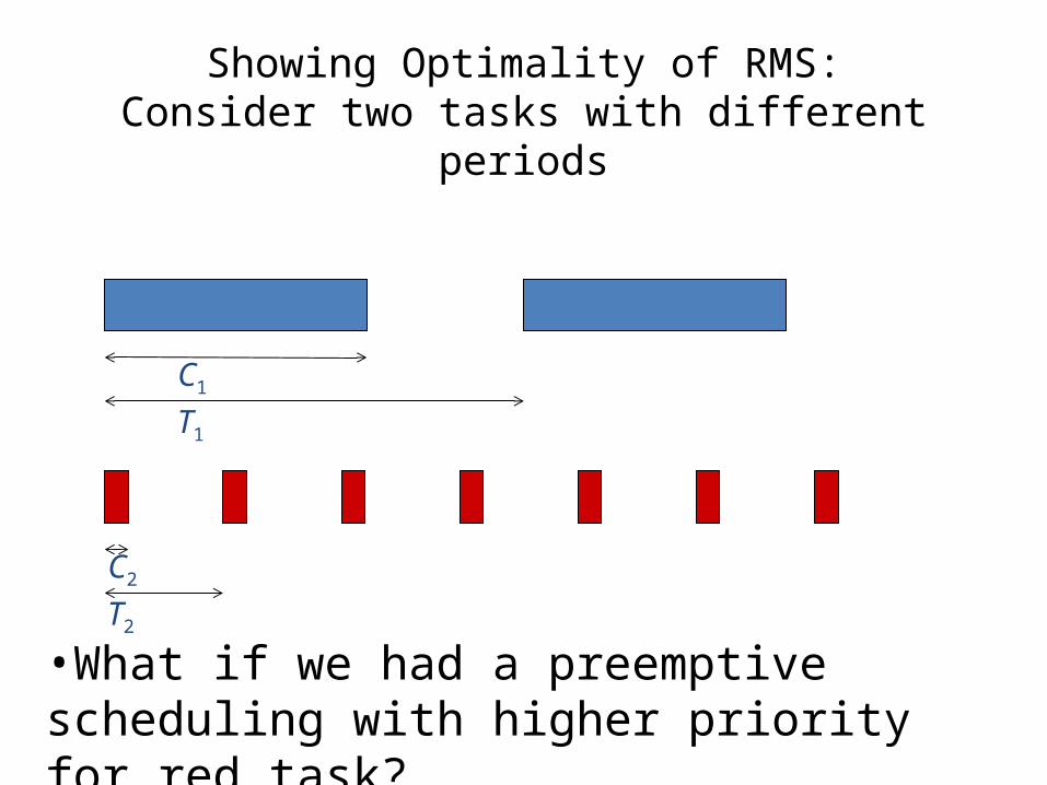
Showing Optimality of RMS:Consider two tasks with different periods
•What if we had a preemptive scheduling with higher priority for red task?
C1
T1
C2
T2
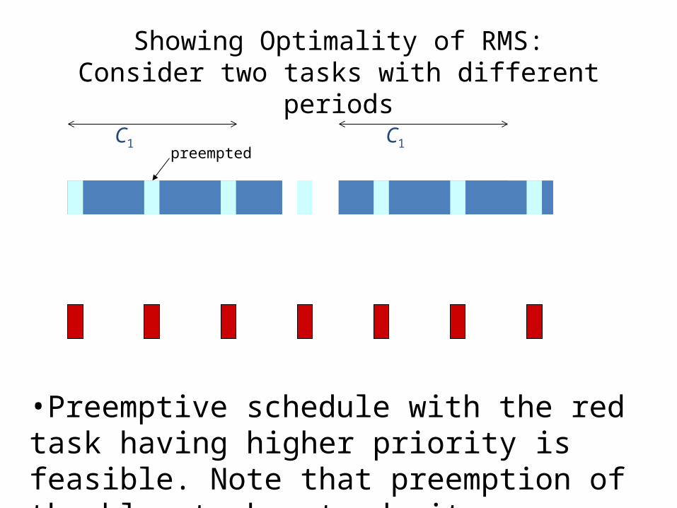
Showing Optimality of RMS:Consider two tasks with different periods
•Preemptive schedule with the red task having higher priority is feasible. Note that preemption of the blue task extends its completion time.
preemptedC1 C1
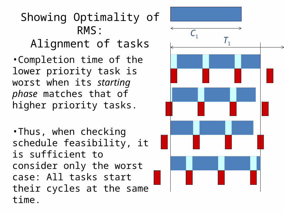
Showing Optimality of RMS:Alignment of tasks
•Completion time of the lower priority task is worst when its starting phase matches that of higher priority tasks.
•Thus, when checking schedule feasibility, it is sufficient to consider only the worst case: All tasks start their cycles at the same time.
T1
C1
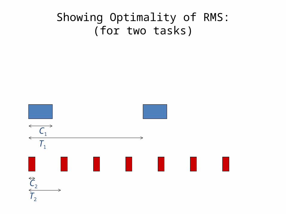
Showing Optimality of RMS:(for two tasks)
•It is sufficient to show that if a non-RMS schedule is feasible, then the RMS schedule is feasible.•Consider two tasks as follows:
C1
T1
C2
T2
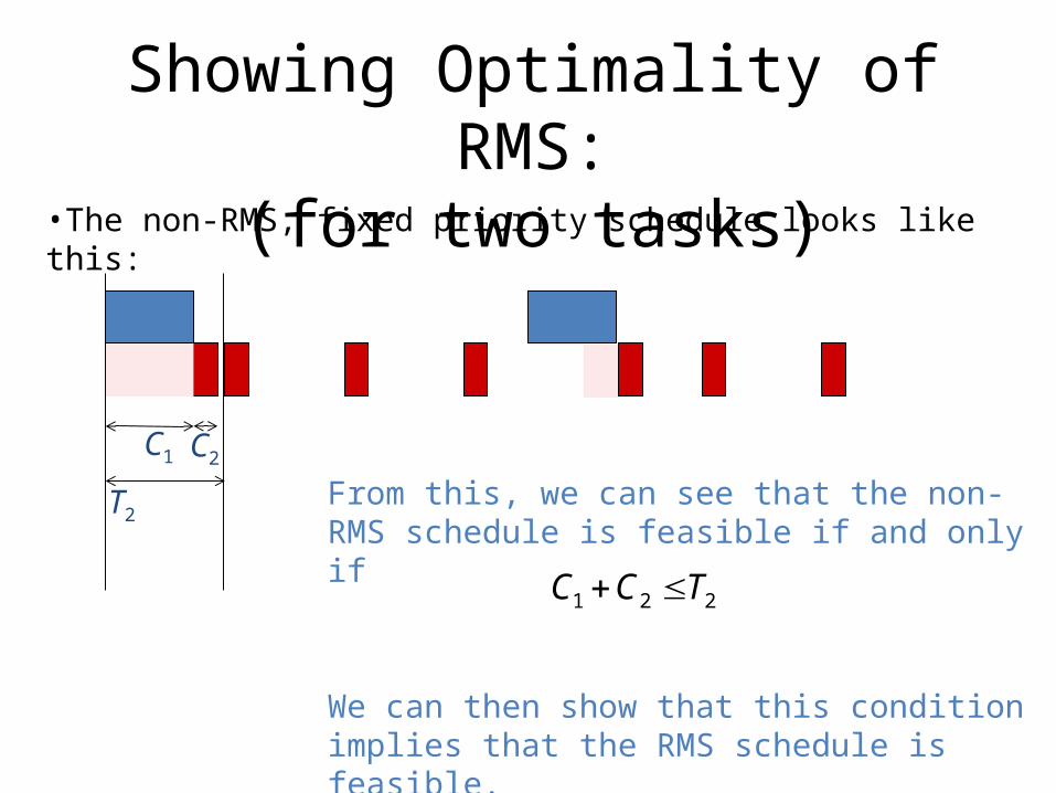
Showing Optimality of RMS:(for two tasks)
•The non-RMS, fixed priority schedule looks like this:
T2
C2C1
From this, we can see that the non-RMS schedule is feasible if and only if
We can then show that this condition implies that the RMS schedule is feasible.
221 TCC
Showing Optimality of RMS:(for two tasks)
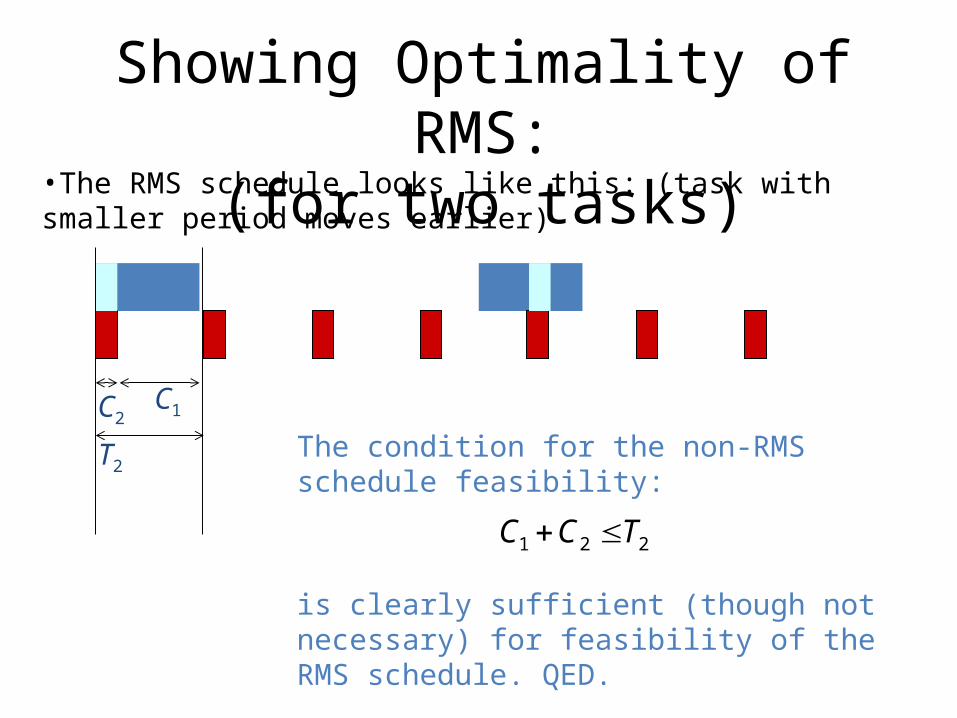
•The RMS schedule looks like this: (task with smaller period moves earlier)
T2
C2C1
The condition for the non-RMS schedule feasibility:
is clearly sufficient (though not necessary) for feasibility of the RMS schedule. QED.
221 TCC
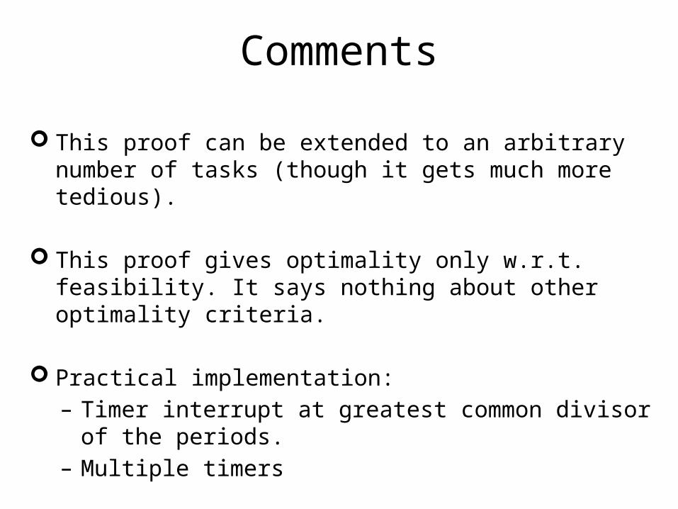
Comments
This proof can be extended to an arbitrary number of tasks (though it gets much more tedious).
This proof gives optimality only w.r.t. feasibility. It says nothing about other optimality criteria.
Practical implementation:– Timer interrupt at greatest common divisor of the periods.– Multiple timers
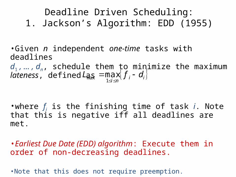
Deadline Driven Scheduling:1. Jackson’s Algorithm: EDD (1955)
•Given n independent one-time tasks with deadlinesd1 , … , dn, schedule them to minimize the maximum lateness, defined as
•where fi is the finishing time of task i. Note that this is negative iff all deadlines are met.
•Earliest Due Date (EDD) algorithm: Execute them in order of non-decreasing deadlines.
•Note that this does not require preemption.
iini
dfL 1
max max
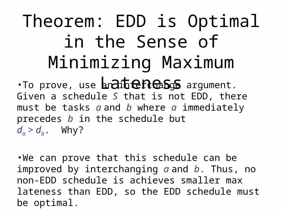
Theorem: EDD is Optimal in the Sense of Minimizing Maximum
Lateness•To prove, use an interchange argument. Given a schedule S that is not EDD, there must be tasks a and b where a immediately precedes b in the schedule but da > db. Why?
•We can prove that this schedule can be improved by interchanging a and b. Thus, no non-EDD schedule is achieves smaller max lateness than EDD, so the EDD schedule must be optimal.
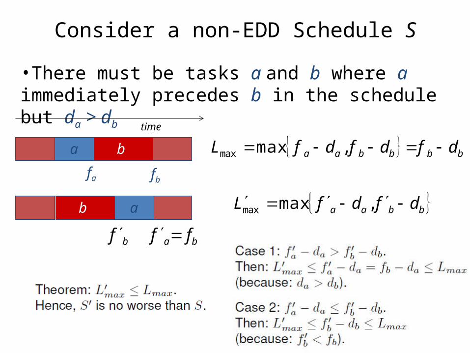
Consider a non-EDD Schedule S
•There must be tasks a and b where a immediately precedes b in the schedule but da > db
a b
fa fb
time
bbbbaa dfdfdfL ,maxmax
ab
ba ff bf
bbaa dfdfL ,maxmax
Deadline Driven Scheduling:1. Horn’s algorithm: EDF (1974)
•Extend EDD by allowing tasks to “arrive” (become ready) at any time.
•Earliest deadline first (EDF): Given a set of n independent tasks with arbitrary arrival times, any algorithm that at any instant executes the task with the earliest absolute deadline among all arrived tasks is optimal w.r.t. minimizing the maximum lateness.
•Proof uses a similar interchange argument.
RMS vs. EDF? Which one is better?
•What are the pros and cons of each?
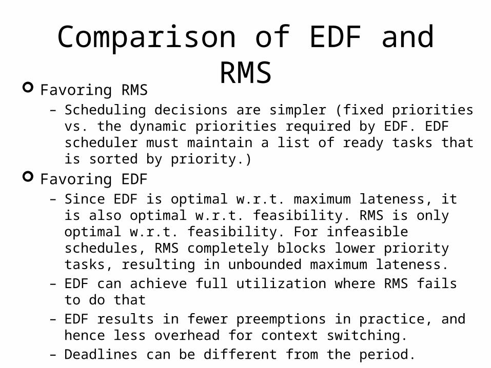
Comparison of EDF and RMS
Favoring RMS– Scheduling decisions are simpler (fixed priorities vs. the dynamic
priorities required by EDF. EDF scheduler must maintain a list of ready tasks that is sorted by priority.)
Favoring EDF– Since EDF is optimal w.r.t. maximum lateness, it is also optimal
w.r.t. feasibility. RMS is only optimal w.r.t. feasibility. For infeasible schedules, RMS completely blocks lower priority tasks, resulting in unbounded maximum lateness.
– EDF can achieve full utilization where RMS fails to do that– EDF results in fewer preemptions in practice, and hence less
overhead for context switching.– Deadlines can be different from the period.
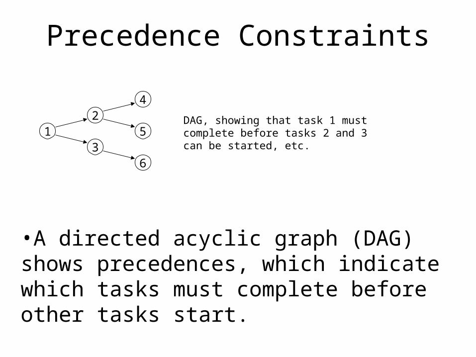
Precedence Constraints
•A directed acyclic graph (DAG) shows precedences, which indicate which tasks must complete before other tasks start.
12
3
4
5
6
DAG, showing that task 1 must complete before tasks 2 and 3 can be started, etc.

Example: EDF Schedule
•Is this feasible? Is it optimal?
12
3
4
5
6C1 = 1d1 = 2 C3 = 1
d3 = 4
C2 = 1d2 = 5
C4 = 1d4 = 3
C5 = 1d5 = 5
C6 = 1d6 = 6

EDF is not optimal under precedence constraints
•The EDF schedule chooses task 3 at time 1 because it has an earlier deadline. This choice results in task 4 missing its deadline.
•Is there a feasible schedule?
12
3
4
5
6C1 = 1d1 = 2 C3 = 1
d3 = 4
C2 = 1d2 = 5
C4 = 1d4 = 3
C5 = 1d5 = 5
C6 = 1d6 = 6
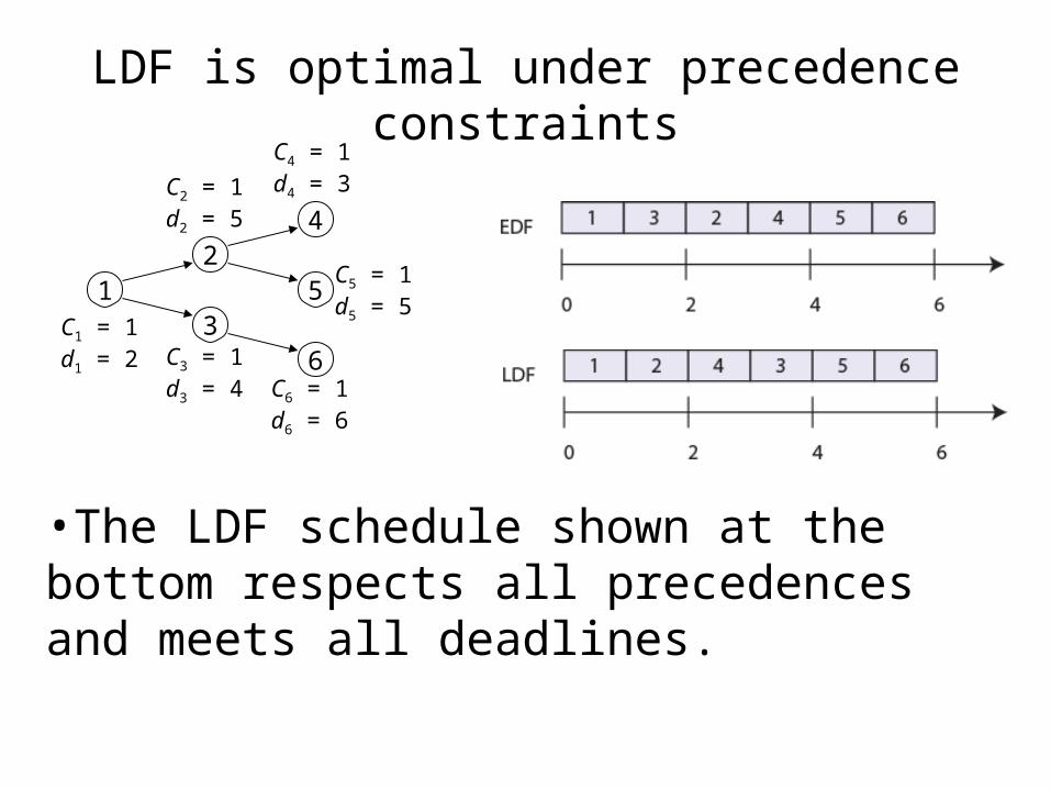
LDF is optimal under precedence constraints
•The LDF schedule shown at the bottom respects all precedences and meets all deadlines.
12
3
4
5
6C1 = 1d1 = 2 C3 = 1
d3 = 4
C2 = 1d2 = 5
C4 = 1d4 = 3
C5 = 1d5 = 5
C6 = 1d6 = 6
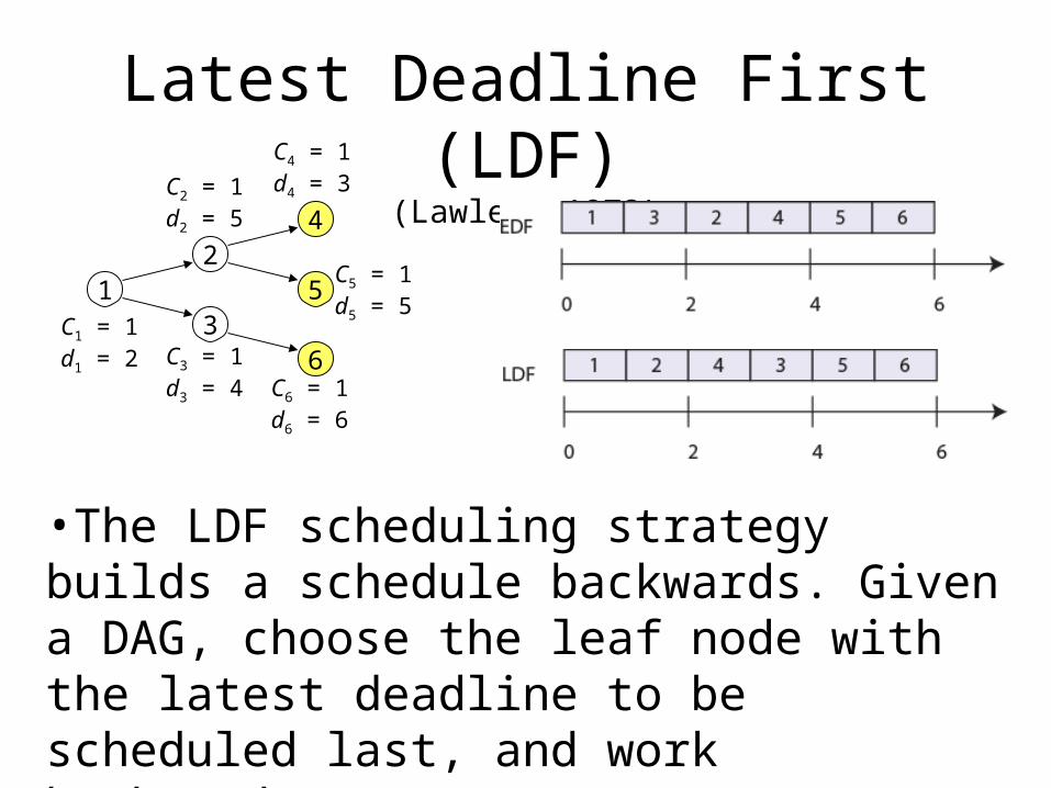
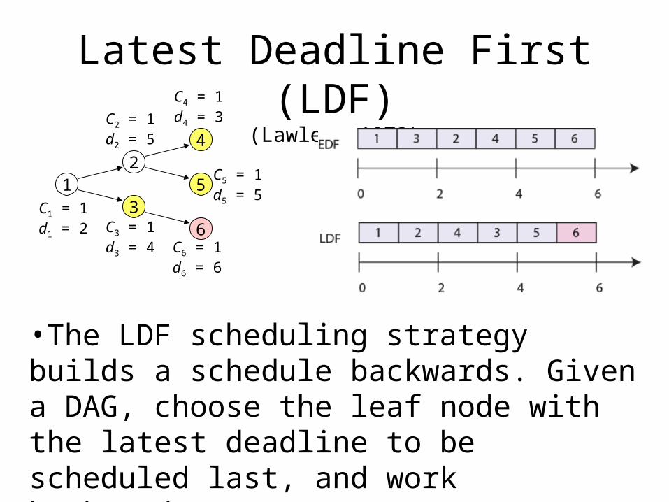
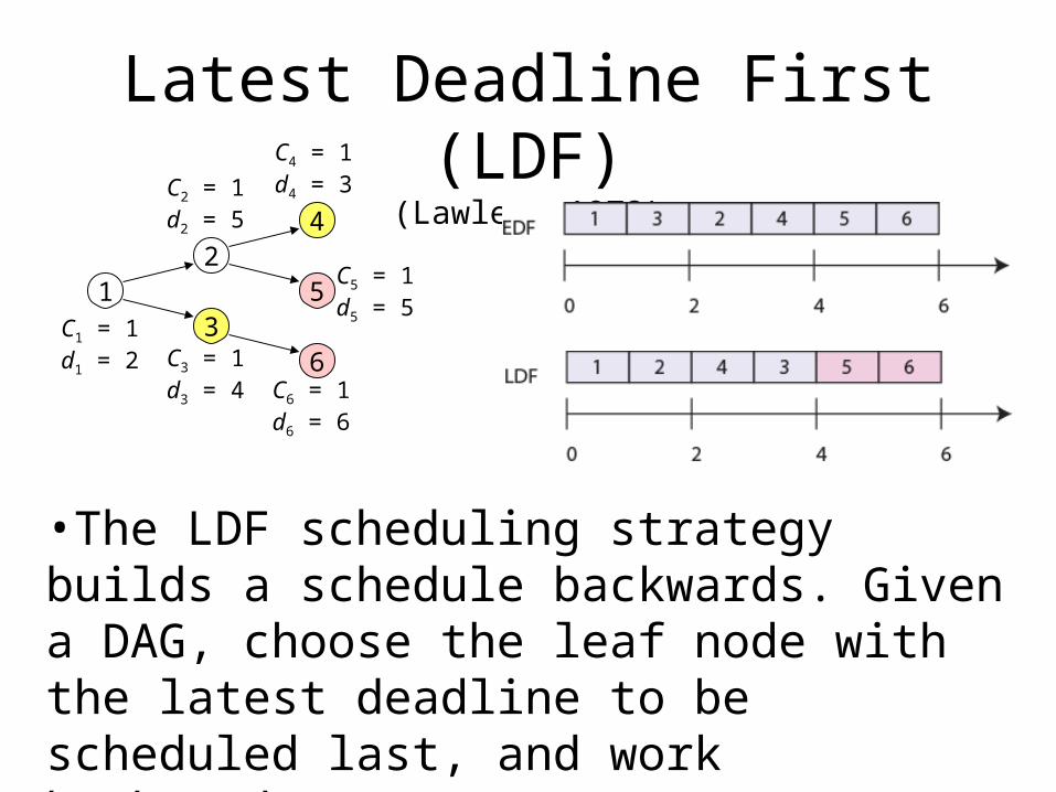
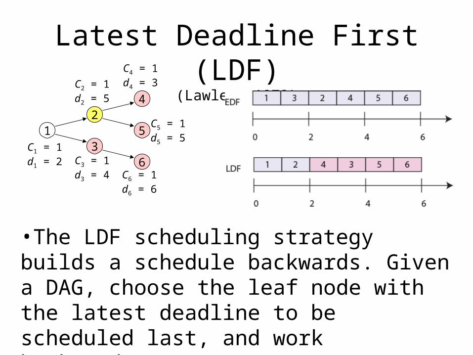
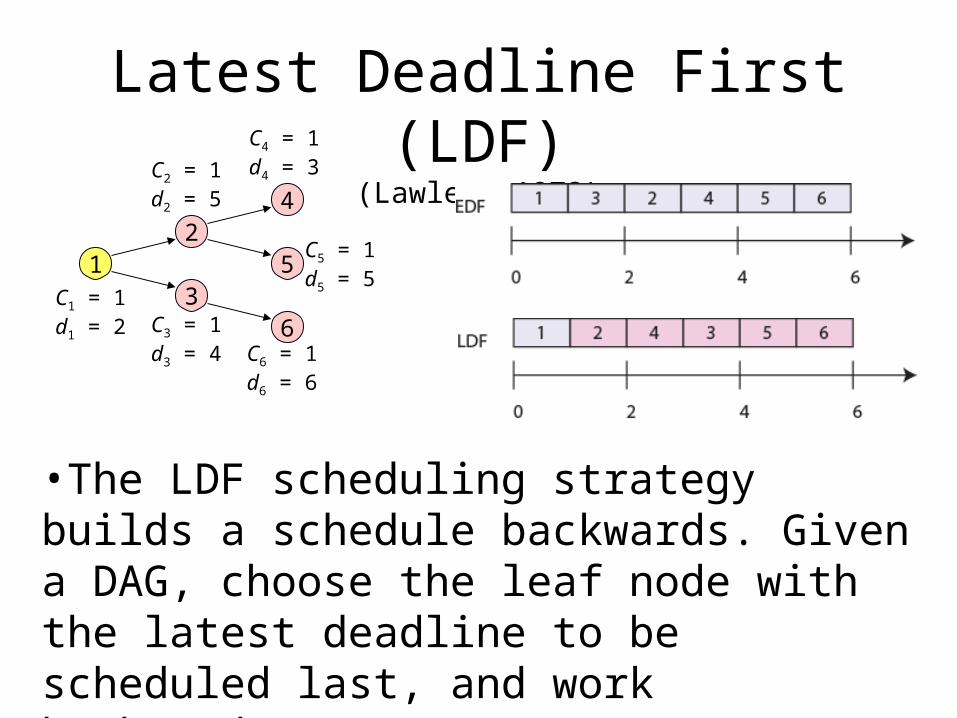
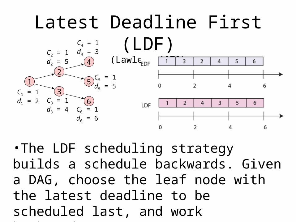
Latest Deadline First (LDF)(Lawler, 1973)
•The LDF scheduling strategy builds a schedule backwards. Given a DAG, choose the leaf node with the latest deadline to be scheduled last, and work backwards.
12
3
4
5
6C1 = 1d1 = 2 C3 = 1
d3 = 4
C2 = 1d2 = 5
C4 = 1d4 = 3
C5 = 1d5 = 5
C6 = 1d6 = 6
Latest Deadline First (LDF)(Lawler, 1973)
•The LDF scheduling strategy builds a schedule backwards. Given a DAG, choose the leaf node with the latest deadline to be scheduled last, and work backwards.
12
3
4
5
6C1 = 1d1 = 2 C3 = 1
d3 = 4
C2 = 1d2 = 5
C4 = 1d4 = 3
C5 = 1d5 = 5
C6 = 1d6 = 6
Latest Deadline First (LDF)(Lawler, 1973)
•The LDF scheduling strategy builds a schedule backwards. Given a DAG, choose the leaf node with the latest deadline to be scheduled last, and work backwards.
12
3
4
5
6C1 = 1d1 = 2 C3 = 1
d3 = 4
C2 = 1d2 = 5
C4 = 1d4 = 3
C5 = 1d5 = 5
C6 = 1d6 = 6

Latest Deadline First (LDF)(Lawler, 1973)
•The LDF scheduling strategy builds a schedule backwards. Given a DAG, choose the leaf node with the latest deadline to be scheduled last, and work backwards.
12
3
4
5
6C1 = 1d1 = 2 C3 = 1
d3 = 4
C2 = 1d2 = 5
C4 = 1d4 = 3
C5 = 1d5 = 5
C6 = 1d6 = 6
Latest Deadline First (LDF)(Lawler, 1973)
•The LDF scheduling strategy builds a schedule backwards. Given a DAG, choose the leaf node with the latest deadline to be scheduled last, and work backwards.
12
3
4
5
6C1 = 1d1 = 2 C3 = 1
d3 = 4
C2 = 1d2 = 5
C4 = 1d4 = 3
C5 = 1d5 = 5
C6 = 1d6 = 6
Latest Deadline First (LDF)(Lawler, 1973)
•The LDF scheduling strategy builds a schedule backwards. Given a DAG, choose the leaf node with the latest deadline to be scheduled last, and work backwards.
12
3
4
5
6C1 = 1d1 = 2 C3 = 1
d3 = 4
C2 = 1d2 = 5
C4 = 1d4 = 3
C5 = 1d5 = 5
C6 = 1d6 = 6
Latest Deadline First (LDF)(Lawler, 1973)
•The LDF scheduling strategy builds a schedule backwards. Given a DAG, choose the leaf node with the latest deadline to be scheduled last, and work backwards.
12
3
4
5
6C1 = 1d1 = 2 C3 = 1
d3 = 4
C2 = 1d2 = 5
C4 = 1d4 = 3
C5 = 1d5 = 5
C6 = 1d6 = 6
Latest Deadline First (LDF)(Lawler, 1973)
•LDF is optimal in the sense that it minimizes the maximum lateness.
•It does not require preemption. (We’ll see that EDF does.)
•However, it requires that all tasks be available and their precedences known before any task is executed.
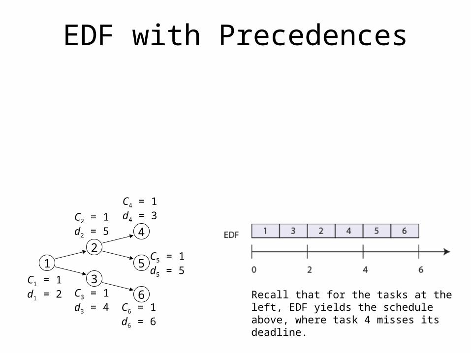
EDF with Precedences•With a preemptive scheduler, EDF can be modified to account for precedences and to allow tasks to arrive at arbitrary times. Simply adjust the deadlines and arrival times according to the precedences.
12
3
4
5
6C1 = 1d1 = 2 C3 = 1
d3 = 4
C2 = 1d2 = 5
C4 = 1d4 = 3
C5 = 1d5 = 5
C6 = 1d6 = 6
Recall that for the tasks at the left, EDF yields the schedule above, where task 4 misses its deadline.

Optimality•EDF with precedences is optimal in the sense of minimizing the maximum lateness.
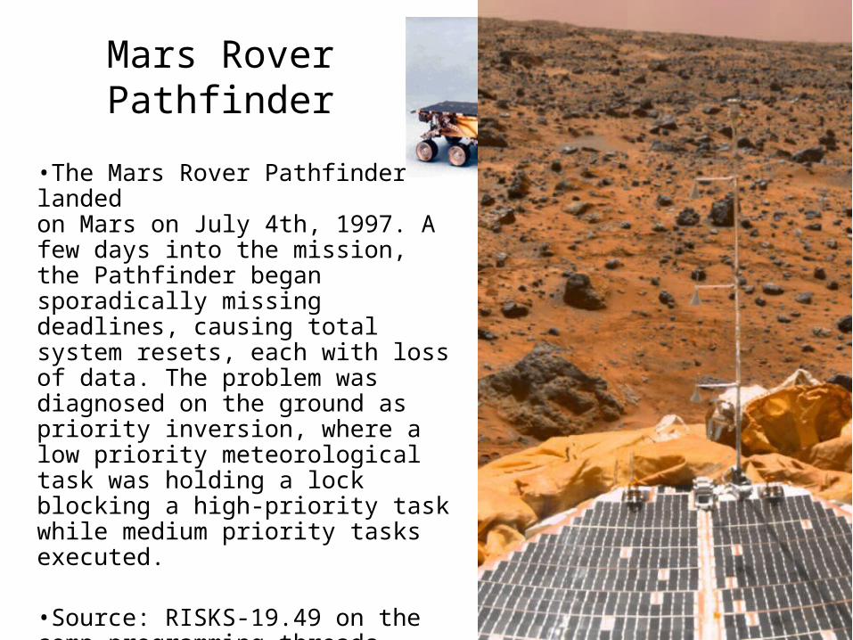
Mars Rover Pathfinder
•The Mars Rover Pathfinder landedon Mars on July 4th, 1997. A few days into the mission, the Pathfinder began sporadically missing deadlines, causing total system resets, each with loss of data. The problem was diagnosed on the ground as priority inversion, where a low priority meteorological task was holding a lock blocking a high-priority task while medium priority tasks executed.
•Source: RISKS-19.49 on the comp.programming.threads newsgroup, December 07, 1997, by Mike Jones ([email protected]).
How do we fix this?
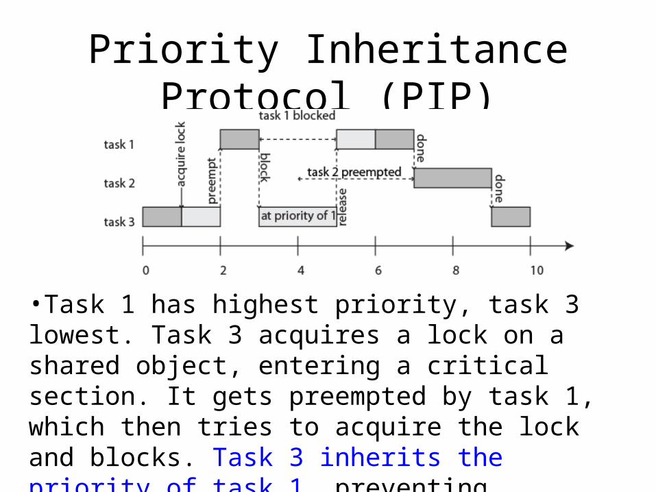
Priority Inheritance Protocol (PIP)
(Sha, Rajkumar, Lehoczky, 1990)
•Task 1 has highest priority, task 3 lowest. Task 3 acquires a lock on a shared object, entering a critical section. It gets preempted by task 1, which then tries to acquire the lock and blocks. Task 3 inherits the priority of task 1, preventing preemption by task 2.
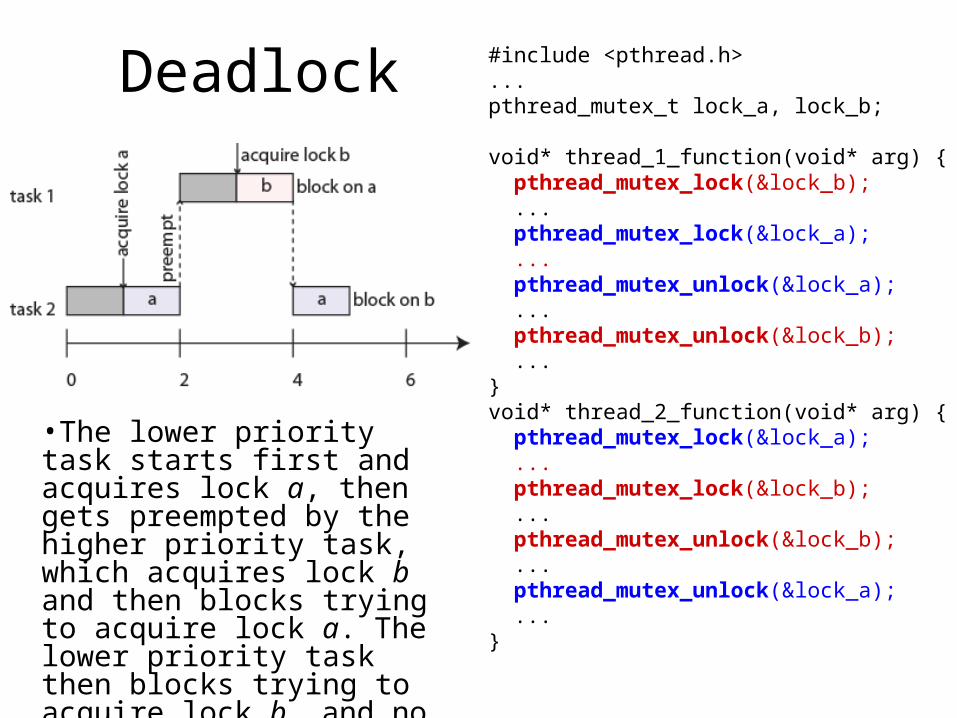
Deadlock #include <pthread.h>...pthread_mutex_t lock_a, lock_b;
void* thread_1_function(void* arg) { pthread_mutex_lock(&lock_b); ... pthread_mutex_lock(&lock_a); ... pthread_mutex_unlock(&lock_a); ... pthread_mutex_unlock(&lock_b); ...}void* thread_2_function(void* arg) { pthread_mutex_lock(&lock_a); ... pthread_mutex_lock(&lock_b); ... pthread_mutex_unlock(&lock_b); ... pthread_mutex_unlock(&lock_a); ...}
•The lower priority task starts first and acquires lock a, then gets preempted by the higher priority task, which acquires lock b and then blocks trying to acquire lock a. The lower priority task then blocks trying to acquire lock b, and no further progress is possible.
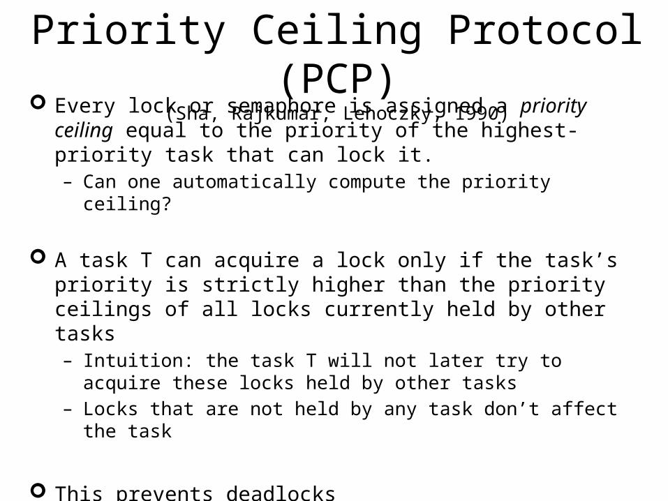
Priority Ceiling Protocol (PCP)(Sha, Rajkumar, Lehoczky, 1990)
Every lock or semaphore is assigned a priority ceiling equal to the priority of the highest-priority task that can lock it.– Can one automatically compute the priority ceiling?
A task T can acquire a lock only if the task’s priority is strictly higher than the priority ceilings of all locks currently held by other tasks– Intuition: the task T will not later try to acquire these locks held by
other tasks – Locks that are not held by any task don’t affect the task
This prevents deadlocks There are extensions supporting dynamic priorities and dynamic
creations of locks (stack resource policy)

Priority Ceiling Protocol
•In this version, locks a and b have priority ceilings equal to the priority of task 1. At time 3, task 1 attempts to lock b, but it can’t because task 2 currently holds lock a, which has priority ceiling equal to the priority of task 1.
#include <pthread.h>...pthread_mutex_t lock_a, lock_b;
void* thread_1_function(void* arg) { pthread_mutex_lock(&lock_b); ... pthread_mutex_lock(&lock_a); ... pthread_mutex_unlock(&lock_a); ... pthread_mutex_unlock(&lock_b); ...}void* thread_2_function(void* arg) { pthread_mutex_lock(&lock_a); ... pthread_mutex_lock(&lock_b); ... pthread_mutex_unlock(&lock_b); ... pthread_mutex_unlock(&lock_a); ...}
Brittleness•In general, all thread scheduling algorithms are brittle: Small changes can have big, unexpected consequences.
•I will illustrate this with multiprocessor (or multicore) schedules.
Theorem (Richard Graham, 1976): If a task set with fixed priorities, execution times, and precedence constraints is scheduled according to priorities on a fixed number of processors, then increasing the number of processors, reducing execution times, or weakening precedence constraints can increase the schedule length.

Richard’s Anomalies
•What happens if you increase the number of processors to four?
1
2
3
4
9
8
9 tasks with precedences and the shown execution times, where lower numbered tasks have higher priority than higher numbered tasks. Priority-based 3 processor schedule:
7
6
5
C1 = 3
C2 = 2
C3 = 2
C4 = 2
C9 = 9
C8 = 4
C7 = 4
C6 = 4
C5 = 4
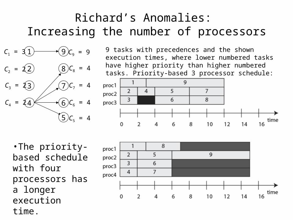
Richard’s Anomalies: Increasing the number of processors
•The priority-based schedule with four processors has a longer execution time.
1
2
3
4
9
8
9 tasks with precedences and the shown execution times, where lower numbered tasks have higher priority than higher numbered tasks. Priority-based 3 processor schedule:
7
6
5
C1 = 3
C2 = 2
C3 = 2
C4 = 2
C9 = 9
C8 = 4
C7 = 4
C6 = 4
C5 = 4
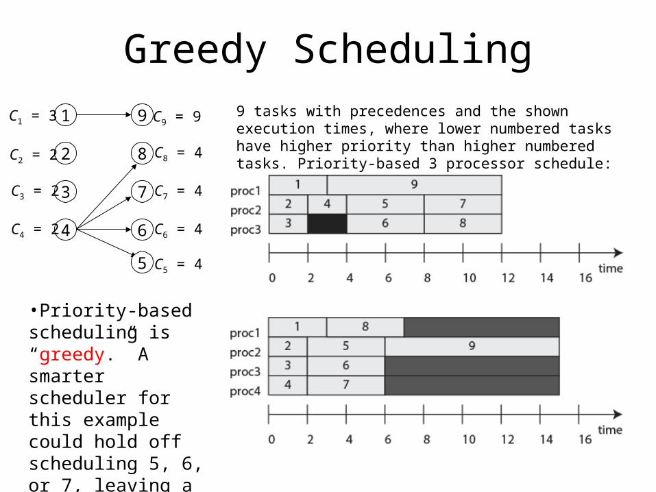
Greedy Scheduling
•Priority-based scheduling is “greedy.” A smarter scheduler for this example could hold off scheduling 5, 6, or 7, leaving a processor idle for one time unit.
1
2
3
4
9
8
9 tasks with precedences and the shown execution times, where lower numbered tasks have higher priority than higher numbered tasks. Priority-based 3 processor schedule:
7
6
5
C1 = 3
C2 = 2
C3 = 2
C4 = 2
C9 = 9
C8 = 4
C7 = 4
C6 = 4
C5 = 4
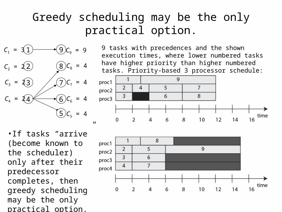
Greedy scheduling may be the only practical option.
•If tasks “arrive” (become known to the scheduler) only after their predecessor completes, then greedy scheduling may be the only practical option.
1
2
3
4
9
8
9 tasks with precedences and the shown execution times, where lower numbered tasks have higher priority than higher numbered tasks. Priority-based 3 processor schedule:
7
6
5
C1 = 3
C2 = 2
C3 = 2
C4 = 2
C9 = 9
C8 = 4
C7 = 4
C6 = 4
C5 = 4

Richard’s Anomalies
•What happens if you reduce all computation times by 1?
1
2
3
4
9
8
9 tasks with precedences and the shown execution times, where lower numbered tasks have higher priority than higher numbered tasks. Priority-based 3 processor schedule:
7
6
5
C1 = 3
C2 = 2
C3 = 2
C4 = 2
C9 = 9
C8 = 4
C7 = 4
C6 = 4
C5 = 4
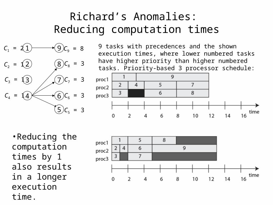
Richard’s Anomalies: Reducing computation times
•Reducing the computation times by 1 also results in a longer execution time.
1
2
3
4
9
8
9 tasks with precedences and the shown execution times, where lower numbered tasks have higher priority than higher numbered tasks. Priority-based 3 processor schedule:
7
6
5
C1 = 2
C2 = 1
C3 = 1
C4 = 1
C9 = 8
C8 = 3
C7 = 3
C6 = 3
C5 = 3
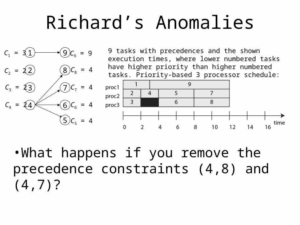
Richard’s Anomalies
•What happens if you remove the precedence constraints (4,8) and (4,7)?
1
2
3
4
9
8
9 tasks with precedences and the shown execution times, where lower numbered tasks have higher priority than higher numbered tasks. Priority-based 3 processor schedule:
7
6
5
C1 = 3
C2 = 2
C3 = 2
C4 = 2
C9 = 9
C8 = 4
C7 = 4
C6 = 4
C5 = 4
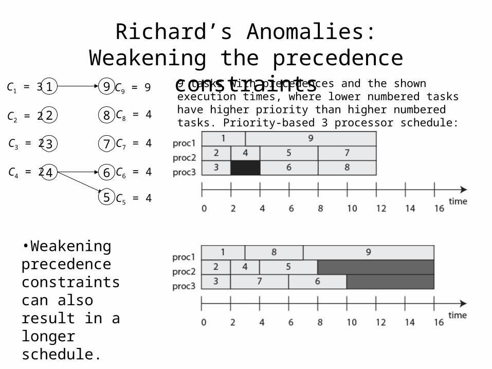
Richard’s Anomalies:Weakening the precedence constraints
•Weakening precedence constraints can also result in a longer schedule.
1
2
3
4
9
8
9 tasks with precedences and the shown execution times, where lower numbered tasks have higher priority than higher numbered tasks. Priority-based 3 processor schedule:
7
6
5
C1 = 3
C2 = 2
C3 = 2
C4 = 2
C9 = 9
C8 = 4
C7 = 4
C6 = 4
C5 = 4
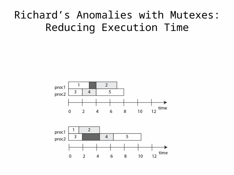
Richard’s Anomalies with Mutexes:Reducing Execution Time
•Assume tasks 2 and 4 share the same resource in exclusive mode, and tasks are statically allocated to processors. Then if the execution time of task 1 is reduced, the schedule length increases:
Conclusion•Timing behavior under all known task scheduling strategies is brittle. Small changes can have big (and unexpected) consequences.
•Unfortunately, since execution times are so hard to predict, such brittleness can result in unexpected system failures.

WRAP UP
For next time
Exam Review