Embed Size (px)
Citation preview
MULTISTATIONARITY IN SEQUENTIAL DISTRIBUTED MULTISITEPHOSPHORYLATION NETWORKS
KATHARINA HOLSTEIN, DIETRICH FLOCKERZI AND CARSTEN CONRADI
Abstract. Multisite phosphorylation networks are encountered in many intracellular processeslike signal transduction, cell-cycle control or nuclear signal integration. In this contribution net-works describing the phosphorylation and dephosphorylation of a protein at n sites in a sequentialdistributive mechanism are considered. Multistationarity (i.e. the existence of at least two pos-itive steady state solutions of the associated polynomial dynamical system) has been analyzedand established in several contributions. It is, for example, known that there exist values for therate constants where multistationarity occurs. However, nothing else is known about these rateconstants.
Here we present a sign condition that is necessary and sufficient for multistationarity in n-site sequential, distributive phosphorylation. We express this sign condition in terms of linearsystems and show that solutions of these systems define rate constants where multistationarity ispossible. We then present, for n ≥ 2, a collection of feasible linear systems and hence give a newand independent proof that multistationarity is possible for n ≥ 2. Moreover, our results allowto explicitly obtain values for the rate constants where multistationarity is possible. Hence webelieve that, for the first time, a systematic exploration of the region in parameter space wheremultistationarity occurs has become possible. One consequence of our work is that, for any pairof steady states, the ratio of the steady state concentrations of kinase-substrate complexes equalsthat of phosphatase-substrate complexes.
Keywords: sequential distributed phosphorylation; mass-action kinetics; multistationarity; signcondition; rate constants
1. Introduction
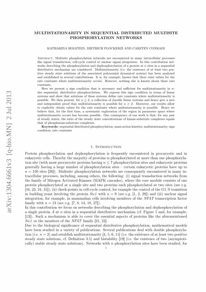
Protein phosphorylation and dephosphorylation is frequently encountered in procaryotic and ineukaryotic cells. Thereby the majority of proteins is phosphorylated at more than one phosphoryla-tion site (with most procaryotic proteins having n ≤ 7 phosphorylation sites and eukaryotic proteinsgenerally having a large number of phosphorylation sites – certain eukaryotic proteins have up ton = 150 sites [26]). Multisite phosphorylation networks are consequently encountered in many in-tracellular processes, including, among others, the following: (i) signal transduction networks fromthe family of Mitogen Activated Kinases (MAPK cascades), where the core module consists of oneprotein phosphorylated at a single site and two proteins each phosphorylated at two sites (see e.g.[16, 23, 24, 31]); (ii) check-points in cell-cycle control, for example the control of the G1/S transitionin budding yeast involving the protein Sic1 with n = 9 (see e.g. [1, 2, 28]) and (iii) nuclear signalintegration, for example, in mammalian cells involving members of the NFAT transcription factorfamily with n = 13 (see e.g. [7, 8, 14, 18, 27]).In this contribution we focus on networks describing the phosphorylation and dephosphorylation ofa single protein A at n sites in a sequential distributive mechanism (cf. Figure 1 and, for example,[13]). Such a mechanism is able to cover the essential aspects of proteins like the aforementionedSic1 or the members of the NFAT family [21, 22].Due to the biological significance of sequential distributive phosphorylation, mathematical modelshave been studied in a variety of publications. Several publications deal with double phosphoryla-tion (i.e. n = 2) and establish multistationarity [4, 5, 6, 11] (i.e. the existence of at least two positivesteady state solutions, cf. Definition 3.5) and bistability [19] (i.e. the existence of two (asymptoti-cally) stable steady state solutions). Networks with n phosphorylation sites have been studied, for
1
arX
iv:1
304.
6661
v3 [
q-bi
o.M
N]
2 J
ul 2
013
2 KATHARINA HOLSTEIN, DIETRICH FLOCKERZI AND CARSTEN CONRADI
Figure 1. Network describing the sequential distributive phosphorylation and de-phosphorylation of protein A at n-sites by a kinase E1 a phosphatase E2. Thephosphorylated forms of A are denoted by the subscript nP (denoting the numberof phosphorylated sites).
example, in [21, 22], where bistability is demonstrated numerically and in [12], where it is arguedthat even though bistability is in principle possible, it is unlikely to occur in-vivo.The set of positive steady states of networks with n phosphorylation sites has been studied alge-braically in [25] and in [20]. In [25] the set of positive steady states of the more general class of socalled post translational modification networks (with n-site sequential distributive phosphorylationas a special case) is analyzed. Such networks admit a rational parameterization of the set of pos-itive steady states. And in [20] it is shown that for n-site sequential distributive phosphorylationthis set is defined by a binomial ideal. Hence n-site sequential distributive phosphorylation is aninstance of a Chemical Reaction System with toric steady states. In [20] a condition for multista-tionarity in these reaction systems is given in terms of a sign condition on elements of two linearsubspaces. Based on the results presented in [3, 4], this condition can be restated in terms of linearsystems: to decide the sign condition, a large set of linear systems has to be examined and multi-stationarity is possible, if and only if at least one of these is feasible (cf. [20, Theorem 5.5] and [3,Lemma 2 & Theorem 2]).The number of steady states in general n-site sequential distributive phosphorylation has beenstudied in [30]. There upper and lower bounds have been established: there exist parameter valuessuch that, for n even (odd), there are at least n+1 (n) steady states. And for all (positive) parametervalues there are at most 2 n − 1 steady states. Hence multistationarity has been established forsequential distributive phosphorylation in [30]. However, no information other than existence isgiven about the parameter values where multistationarity is possible. In this contribution we addressthis question: we present for every n ≥ 2 a collection of feasible linear systems and show thatevery solution of one of those systems defines parameter values where multistationarity is possible(together with two positive steady states as witness). Thus these results not only constitute a newand independent proof that multistationarity is possible for n ≥ 2, they additionally enable, forthe first time, a systematic exploration of the region in parameter space where multistationarityis possible. Due to the ubiquity of multisite phosphorylation this may be of potential interest toresearchers working in many fields of (quantitative) biology. For the purpose of finding parametervalues in biologically meaningful ranges we will start with this exploration in [15].We arrive at our main result on the basis of our previous work from [3, 4] and [20]: as in theaforementioned references we derive a sign condition that is necessary and sufficient for the existenceof multistationarity (Theorem 4.2 & 4.6). In contrast to [3, 20] our condition is formulated in termsof the sign patterns generated by two linear subspaces (given as the image of two matrices definedin eqns. (8e) & (17c)). We then exploit the fact that every sign pattern uniquely defines a linearsystem to restate the sign condition in terms of these linear systems: multistationarity is possible,if and only if at least one out of 1
2
(3(3n+3) − 1
)or 2(3n+2) linear systems is feasible depending on
whether some or all components of the two witness steady state vectors have to differ to qualify

MULTISTATIONARITY IN SEQUENTIAL DISTRIBUTED MULTISITE PHOSPHORYLATION NETWORKS 3
for multistationarity, cf. Definition 3.5 and Remark 4.7. For the latter case, we present formulae toconstruct all sign patterns defining feasible linear systems (cf. Theorem 4.10) and show that everysolution of one of these linear systems defines parameter values where multistationarity occurs withtwo positive steady states differing in every component. We show that there are 2 (n− 1)(n+ 2)such sign patterns (cf. Proposition 4.14).This paper is organized as follows: Section 2 introduces some of the basic notations. In Section 3a mass action network is derived from Fig. 1 and the associated dynamical system is defined alongwith a formal definition of multistationarity. In Section 4 the main results address multistationarityin terms of sign patterns defining feasible linear systems (cf. Theorem 4.2 & 4.10). The proofs oftwo of these results have been relegated to separate Sections 5 & 6 for easier reading.
2. Notation
We use the symbol IRm to denote Euclidian m-space, the symbol IRm≥0 to denote the nonnegativeorthant and IRm>0 to denote the interior of the nonnegative orthant. Vectors are considered as columnvectors and, for convenience, usually displayed as row vectors using T to denote the transpose. Forexample, x ∈ IRm will usually be displayed as (x1, . . . , xm)T .For positive vectors x ∈ IRm>0 we use the shorthand notation lnx to denote
lnx := (lnx1, . . . , lnxm)T ∈ IRm. (1a)
Similarly, for x ∈ IRm, we use ex to denote
ex := (ex1 , . . . , exm)T ∈ IRm>0 (1b)
and, for x ∈ IRm with xi 6= 0, i = 1, . . ., m,
x−1 :=
(1
x1, . . . ,
1
xm
)T∈ IRm . (1c)
Finally, xy with x, y ∈ IRm≥0 will be defined by
xy :=m∏i=1
xyii ∈ IRm≥0 . (1d)
The set of real (p × q)-matrices with p rows and q columns will be denoted by IRp×q. For p-dimensional column vectors s(j) = (s1j , ..., spj)
T ∈ IRp, j = 0, 1, ..., q, we denote the p(q + 1)-dimensional column vector (s10, ..., sp0, s11, ..., sp1, ....... , s1q, ..., spq)
T by
col(s(0), ..., s(q)) ∈ IRp(q+1) with the matrix (s(0), ...s(q)) ∈ IRp×(q+1) . (2)
3. Mathematical models of n-site sequential distributive phosphorylation
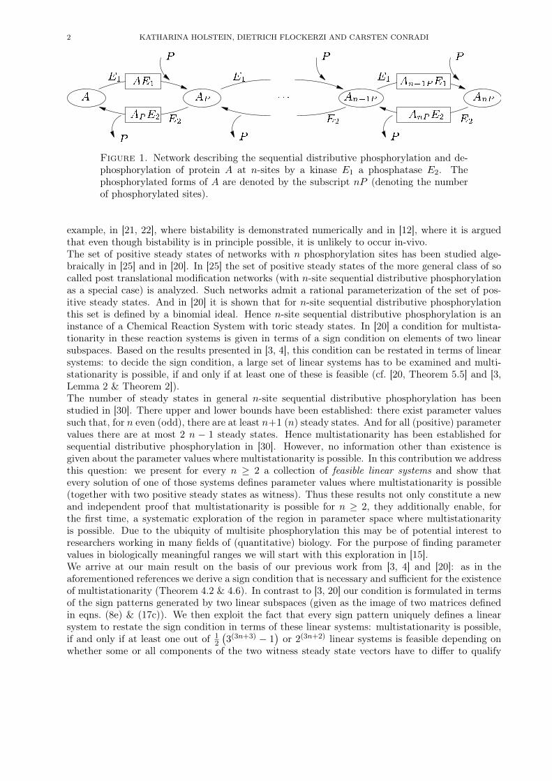
Here we first introduce the notation used to describe dynamical systems defined by mass actionnetworks by means of the example network depicted in Fig. 2. Then we discuss the mass actionnetwork derived from Fig.1 and present the dynamical system defined by this mass action network.

4 KATHARINA HOLSTEIN, DIETRICH FLOCKERZI AND CARSTEN CONRADI
(a) 1-site phosphorylation
x1E1 +
x2A
k1GGGGGGBFGGGGGG
k2
x4AE1
k3GGGGGGA
x1E1 +
x5AP
x3E2 +
x5AP
l1GGGGGBFGGGGG
l2
x6APE2
l3GGGGGA
x3E2 +
x2A
(b) Mass action network
Figure 2. Phosphorylation of protein A at a single phosphorylation site: processdiagram (A) and mass action network (B).
3.1. Dynamical systems defined by a single phosphorylation network. The network de-picted in Fig. 2 describes the phosphorylation of a protein A at a single site by the kinase E1 and thedephosphorylation of mono-phosphorylated protein AP by the phosphatase E2 (cf. Fig. 2a). Fig-ure 2b contains a mass action network describing this process, where chemical reactions are denotedby arrows pointing from the species that are consumed in a reaction (the educts) to the species thatare produced (the products) and ki (li) denote rate constants. The network consists of 6 species, thekinase E1 (with concentration variable x1), the protein A (x2), the phosphatase E2 (x3), the enzymesubstrate complexes AE1 (x4) and APE2 (x6) and the mono-phosphorylated AP (x5). The networkis composed of 6 reactions, two describing the reversible binding of protein and kinase E1+AAE1,one the irreversible release of mono-phosphorylated protein and kinase AE1→E1 +AP , two the re-versible binding of mono-phosphorylated protein and phosphatase E2 + APAPE2 and one theirreversible release unphosphorylated protein and phosphatase APE2→E2 +A.To every reaction we associate a reaction vector describing the stoichiometry of that reaction. Forexample in the reaction
E1 +Ak1
GGGGGGAAE1
one unit of A (x2) and E1 (x1) are consumed and one unit of AE1 (x4) is produced, which yieldsthe vector
(−1, −1, 0, 1, 0, 0)T .
All in all one obtains six reaction vectors, that we collect as column vectors of the stoichiometricmatrix
S(1) =
−1 1 1 0 0 0−1 1 0 0 0 1
0 0 0 −1 1 11 −1 −1 0 0 00 0 1 −1 1 00 0 0 1 −1 −1
,
where the superscript (1) is used to denote the stoichiometric matrix of a 1-site phosphorylationnetwork. Columns 1 and 2 of S(1) correspond to the reversible binding of A and E1, column 3 tothe irreversible release of AP and E1, columns 4 and 5 to the reversible binding of AP and E2 andcolumn 6 to the irreversible release of A and E2.Using mass action kinetics the reaction rate ri (i.e. the speed of reaction i) is proportional to theproduct of the concentrations of the educts, for example, the rate r1 = k1 x1 x2 for the reactionE1 + A → AE1. Similarly one obtains r2 = k2 x4 for AE1 → E1 + A, r3 = k3 x4 for AE1 →E1 + AP , r4 = l1 x3 x5 for E2 + AP → APE2, r5 = l2 x6 for APE2 → E2 + AP and r6 = l3 x6 for
MULTISTATIONARITY IN SEQUENTIAL DISTRIBUTED MULTISITE PHOSPHORYLATION NETWORKS 5
APE2 → E2 +A. With x = (x1,. . . , x6)T , κ = (k1, . . . , k3, l1, . . . , l3)T we collect r1, . . . , r6 in thevector
r(1) (κ, x) = (k1 x1 x2, k2 x4, k3 x4, l1 x3 x5, l2 x6, l3 x6)T (3a)
and obtain the dynamical system
x = S(1) r(1) (κ, x) , (3b)
which can be written componentwise as
x1 = (k2 + k3)x4 − k1x1x2,x2 = −k1x1x2 + k2x4 + l3x6,
x3 = (l2 + l3)x6 − l1x3x5,x4 = − (k2 + k3)x4 + k1x1x2, (3c)x5 = k3x4 − l1x3x5 + l2x6,
x6 = − (l2 + l3)x6 + l1x3x5.
Note that the vector r(1) (κ, x) is fully characterized by the vector κ and the exponents of themonomials. We collect those in the rate exponent matrix Y(1) corresponding to the educt complexes(i.e., the ‘left-hand sides’ of the reactions):
Y(1) =
1 0 0 0 0 01 0 0 0 0 00 0 0 1 0 00 1 1 0 0 00 0 0 1 0 00 0 0 0 1 1
. (3d)
Fig. 2 does not consider protein synthesis and degradation, the total amount of protein A is thereforeconstant, that is, one has the conservation relation
x2 + x4 + x5 + x6 = c1,
where c1 is a constant denoting the total concentration of A. The name conservation relation stemsform the fact that the above sum of concentrations is constant along solutions of (3b): from (3c) itis easy to see that x2 (t)+ x4 (t)+ x5 (t)+ x6 (t) = 0 and hence x2 (t)+x4 (t)+x5 (t)+x6 (t) = const.Likewise one has
x1 + x4 = c2 and x3 + x6 = c3,
with constants c2 and c3 denoting the total concentration of E1 and E2, respectively. Conservationrelations are defined by elements of the left kernel of the matrix S(1). One obtains, for example, thefollowing full row-rank matrix
Z(1) =
1 0 0 1 0 00 0 1 0 0 10 1 0 1 1 1
with Z(1) S(1) ≡ 0 where the rows form a basis of the left kernel of S(1).
3.2. The mass action network derived from Figure 1. The mass action network derivedfrom Fig. 1 (with n an arbitrary but fixed positive number) has been described in [20, 30]. Herewe use a similar mathematical description: the network consists of the following chemical species:the protein (substrate) A together with n phosphoforms AP , . . . , AnP ; the kinase E1 togetherwith n kinase-substrate complexes AE1, . . . , An−1P E1 and the phosphatase E2 together with nphosphatase-substrate complexes AP E2, . . . , AnP E2. Hence there is a total of 3n+ 3 species. To

6 KATHARINA HOLSTEIN, DIETRICH FLOCKERZI AND CARSTEN CONRADI
Phos. # Species Var.
0E1 x1A x2E2 x3
1AE1 x4AP x5
AP E2 x6...
iAi−1P E1 x1+3i
AiP x2+3i
AiP E2 x3+3i...
nAn−1P E1 x1+3n
AnP x2+3n
AnP E2 x3+3n
Table 1. Assignment of variables to species
each species, a variable xi denoting its concentration is assigned as depicted in Table 1. We collectall variables in a (3n+ 3)-dimensional vector
x := (x1, . . . , x3n+3)T .
As it will turn out, the chosen labeling entails a simple block structure for the matrices associatedto the dynamical system (11b) of the network in Fig. 1, cf., for example, the block structure (15b)for the generators of the nonnegative cone in the kernel of the stoichiometric matrix.Assuming a distributive mechanism, a single phosphorylation occurs with each encounter of sub-strate and kinase [13] and n phosphorylations therefore require n encounters of substrate and kinaseof the form
E1 +Ai−1P GGGBFGGGAi−1P E1GGGAE1 +AiP , i = 1, . . . , n ,
where A0P = A and A1P = AP . Similarly, n dephosphorylations following a distributive mechanismrequire n encounters of substrate and phosphatase of the form:
E2 +AiP GGGBFGGGAiP E2GGGAE2 +Ai−1P , i = 1, . . . , n .
Each phosphorylation and each dephosphorylation therefore consists of 3 reactions and consequentlythe network consists of 6n reactions. To each reaction we associate a rate constant. We use ki forphosphorylation and li for dephosphorylation reactions and obtain the following reaction network:
E1 +Ai−1Pk3i−2
GGGGGGGGGBFGGGGGGGGG
k3i−1Ai−1P E1
k3iGGGAE1 +AiP , i = 1, . . . , n
E2 +AiPl3i−2
GGGGGGGGBFGGGGGGGG
l3i−1AiP E2
l3iGGGAE2 +Ai−1P , i = 1, . . . , n .
(4)
Using this notation, k3i−2 (l3i−2) denotes the association constant, k3i−1 (l3i−1) the dissociationconstant and k3i (l3i) the catalytic constant of the i-th phosphorylation (dephosphorylation) step.We collect all rate constants in a vector κ defined in the following way:
MULTISTATIONARITY IN SEQUENTIAL DISTRIBUTED MULTISITE PHOSPHORYLATION NETWORKS 7
Definition 3.1 (The vector of rate constants κ).We collect the six rate constants associated to the i-th phosphorylation/dephosphorylation in net-work (4) in a sub-vector
κ(i) := (k3i−2, k3i−1, k3i, l3i−2, l3i−1, l3i)T . (5a)
We then combine the sub-vectors to a 6n-dimensional column vector
κ := col(κ(1), . . . , κ(n)
). (5b)
We conclude this subsection with a brief comment on the notation used to denote (sub-)vectors andmatrices throughout this contribution.
Remark 3.2 (Vector and matrix notation).In the following sections the dimension of vectors is determined by the number of phosphorylationsites n according to the formula 3n + 3. (The vector x, for example, lives in Euclidian IR3n+3, cf.Table 1). We will use the symbol ej to denote elements of the standard basis of Euclidian vectorspaces and use the superscript (i) to distinguish basis vectors of vector spaces of different dimension3i+ 3:
e(i)j . . . denotes elements of the standard basis of IR3i+3. (6)
Likewise for matrices the superscript (i) is used to indicate that the number of rows and/or columnsdepends on an integer i (see, for example, equations (10), (8e), (9d) or (15b) below).Later on we will split vectors of length 3n + 3 into consecutive sub-vectors of length three and wewill use the subscript (i) to denote the i-th sub-vector
x(i) := (x3i+1, x3i+2, x3i+3)T
and we will use x = col(x(0), . . . , x(n)
)to denote that x consists of n+1 such sub-vectors. Likewise
we will split vectors of length 6n into sub-vectors
y(i) := (y6i−5, . . . , y6i)T
of length six and use y = col(y(1), . . . , y(n)
)to denote that y consists of n such sub-vectors. �
3.3. The dynamical system defined by the mass action network (4). Starting with thestoichiometric matrix S(1) and the rate exponent matrix Y(1) defined by the mass action networkdepicted in Fig. 2b one can recursively construct matrices S(n) and Y(n) for the network (4). Usingthe ordering of species and reactions introduced above in Table 1 one obtains S(n) ∈ IR(3n+3)×6n,Y(n) ∈ IR(3n+3)×6n and Z(n) by the following steps:(I) Concerning S(n):
S(1) =
[n11n21
], S(2) =
S(1) n12n22
03×6 n21
, . . . (7a)
S(j) =
S(j−1)n12
03(j−2)×6n22
03×6(j−1) n21
(7b)

8 KATHARINA HOLSTEIN, DIETRICH FLOCKERZI AND CARSTEN CONRADI
for j = 3, ..., n with the following sub-matrices of dimension 3× 6:
n11 =
−1 1 1 0 0 0−1 1 0 0 0 1
0 0 0 −1 1 1
, (8a)
n12 =
−1 1 1 0 0 00 0 0 0 0 00 0 0 −1 1 1
, (8b)
n21 =
1 −1 −1 0 0 00 0 1 −1 1 00 0 0 1 −1 −1
, (8c)
n22 =
0 0 0 0 0 0−1 1 0 0 0 1
0 0 0 0 0 0
. (8d)
For fixed n, the recursive formula (7b) evaluates to
S(n) :=
n11 n12 n12 n12 n12n21 n22 03×6 02·3×6
0(n−2)·3×6
03×6 n21 n22 . . .03×6·2 n21 n22
03×6·3 n21...
. . .03×6·(n−1) n21
∈ IR(3n+3)×6n . (8e)
(II) Concerning Y(n):
Y(1) =[e(1)1 + e
(1)2 e
(1)4 e
(1)4 e
(1)3 + e
(1)5 e
(1)6 e
(1)6
], (9a)
Y(j) =
[Y(j−1)
03×6(j−1)e(j)1 + e
(j)3j−1 e
(j)3j+1 e
(j)3j+1 e
(j)3 + e
(j)3j+2 e
(j)3j+3 e
(j)3j+3
](9b)
for j = 2, ..., n with Y(1) ∈ IR6×6 (cf. eq.(3d)) and Y(j) ∈ IR(3j+3)×6j . Using
Y0 (i) :=[e(i)1 + e
(i)3i−1 e
(i)3i+1 e
(i)3i+1 e
(i)3 + e
(i)3i+2 e
(i)3i+3 e
(i)3i+3
]∈ IR(3i+3)×6 , (9c)
the recursive formula (9b) evaluates to
Y(n)T :=
Y0 (1)T 06·1×3 06·2×3 06·3×306·n×3
Y0 (2)T
Y0 (3)T
. . .Y0 (n− 1)T
Y0 (n)T
. (9d)
(III) Concerning Z(n):

MULTISTATIONARITY IN SEQUENTIAL DISTRIBUTED MULTISITE PHOSPHORYLATION NETWORKS 9
Z(n) =
1 0 00 0 10 1 0
1 0 0 1 0 00 0 1 · · · 0 0 11 1 1 1 1 1
︸ ︷︷ ︸
n−times
∈ IR3×(3n+3).(10)
We note that the three rows of Z(n) form a basis for the left kernel of S(n).
Definition 3.3 (Reaction rate vector defined by network (4)).The vector of rate constants κ from (5b) and the columns yi of Y(n) from (9d) define two monomialfunctions Φ(n) : IR3n+3 → IR6n and r(n) (κ, x) : IR3n+3 → IR6n:
Φ(n) (x) := (xy1 , . . . , xy6n)T (11a)
and
r(n) (κ, x) := diag (κ) Φ(n) (x) (11b)
for x ∈ IR3n+3≥0 (cf. (1d)). The 6n-dimensional vector r(n) (κ, x) is called the reaction rate vector.
Together with the stoichiometric matrix S(n) from (8e), the dynamical system, defined by thenetwork (4) of Fig. 1, is then given by
x = S(n) r(n) (κ, x) (12)
Remark 3.4 (The monomial function Φ(n) (x)).Observe that the monomial function Φ(n) (x) in (11b) satisfies
Φ(n) (eµ) = eY(n)T µ , (13a)
1
Φ(n) (x)= Φ(n)
(x−1
)(13b)
for vectors µ ∈ IR3n+3 and x ∈ IR3n+3 with xi 6= 0, i = 1, . . . , 3n+ 3. �
From equation (12) follows that level sets {x ∈ IR3n+3|Z(n) x = const.} are invariant under the flowof (12) as Z(n) x(t) = Z(n) x(0) along solutions x(t) of (12). This observation motivates the classicaldefinition of multistationarity originating in chemical engineering (cf. Figure 3 and, for example, [3,Definition 1&Remark 2] or [9, 10]):
Definition 3.5 (Multistationarity).The system x = S(n) r(n) (κ, x) from (12) is said to exhibit multistationarity if and only if thereexist a positive vector κ ∈ IR6n
>0 and at least two distinct positive vectors a, b ∈ IR3n+3>0 with
S(n) r(n) (κ, a) = 0 (14a)
S(n) r(n) (κ, b) = 0 (14b)
Z(n) a = Z(n) b. (14c)
We conclude this section by a discussion of ker(S(n)
)and of the pointed polyhedral cone ker
(S(n)
)∩
IR3n+3≥0 :

10 KATHARINA HOLSTEIN, DIETRICH FLOCKERZI AND CARSTEN CONRADI
Figure 3. Multistationarity and bistability: While the equation S(n) r(n)(κ, x) = 0often has infinitely many steady state solutions, a solution x(t) of the differentialequation x = S(n) r(n)(κ, x) ‘sees’ only those contained in the level set Lx(0) := {x ∈IR3n+3≥0 |Z(n) x = Z(n) x(0)}. Multistationarity requires at least two positive steady
state solutions in Lx(0), bistability two ‘stable’ positive steady state solutions inLx(0). The triangle in the figure shows such a level set Lx(0) in IR3
≥0 with two stablepositive steady states. The stable manifold (in red) of the third positive steady stategenerates the threshold separating the domains of attraction of the two stable steadystates.
Lemma 3.6 (A nonnegative basis of ker(S(n)
)).
Let n ≥ 2 be given and recall the stoichiometric matrix S(n) as defined in (8e). Let
E =
1 0 11 0 00 0 10 1 10 1 00 0 1
(15a)
and define the 6n× 3n matrix with E on the block diagonal (and zero otherwise):
E(n) :=
E. . .
E
(15b)
Then columns of E(n) form a basis of ker(S(n)
). In addition, the columns of E(n) are generators of
ker(S(n)
)∩ IR3n+3
≥0 .
Proof. First recall the building blocks of S(n), the 3× 6 sub-matrices n11, n21, n12 and n22 (cf. (8)).We show that im
(E(n)
)= ker
(S(n)
)by proving the two inclusions im
(E(n)
)⊆ ker
(S(n)
)and
ker(S(n)
)⊆ im
(E(n)
).
(i) Concerning im(E(n)
)⊆ ker
(S(n)
):
Straightforward computations show that n11E = 03×3, n12E = 03×3, n21E = 03×3 and n22E =03×3. Thus S(n)E(n) = 0(3n+3)×3n.

MULTISTATIONARITY IN SEQUENTIAL DISTRIBUTED MULTISITE PHOSPHORYLATION NETWORKS 11
(ii) Concerning ker(S(n)
)⊆ im
(E(n)
):
We first note that the columns of E form a basis of ker (n11) and ker (n21). Pick any vectorη ∈ ker
(S(n)
)and split it in consecutive sub-vectors of length 6 as described in Remark 3.2:
η = col(η(1), . . . , η(n)
). The vector η satisfies S(n) η = 0, that is (cf. eq.(8e) defining S(n))
n11η(1) +n∑i=2
n12η(i) = 0,
n21η(1) + n22η(2) = 0,
...n21η(n−1) + n22η(n) = 0,
n21η(n) = 0.
From the last equation follows that η(n) ∈ ker(n21) = im (E). The preceding equations then implyη(i) ∈ ker(n21) = im (E), for i = n−1, . . . , 1. Hence η ∈ im
(E(n)
)and thus ker
(S(n)
)⊆ im
(E(n)
).
Finally, concerning the pointed polyhedral cone, observe that a vector η is called a generator of thecone ker
(S(n)
)∩ IR3n+3
≥0 , if and only if η satisfies the following three conditions (cf. for example,[17]):
(i) η ≥ 0 , (ii) S(n) η = 0,
(iii) for generators η1 and η2 of ker(S(n)
)∩ IR3n+3
≥0 one hassupp (η1) ⊆ supp (η2)⇒ η1 = 0 or η1 = αη2 with α > 0,
where the symbol supp (η) denotes the support of a vector η ∈ IR3n+3 (i.e. the set of indices of thenonzero elements). Observe that the column vectors of E satisfy these conditions and recall theblock diagonal structure of E(n). Hence the columns of E(n) satisfy these conditions as well. �
4. Results
In this section we first introduce a condition for multistationarity (cf. Definition 3.5) in terms of signpatterns, followed by a discussion of sign patterns satisfying this condition. The rather technicalproofs of Theorem 4.2 and Theorem 4.10 will be presented in Section 5 and Section 6 respectively.
4.1. A sign condition for multistationarity in the dynamical system (12). We now turnto multistationarity for dynamical systems defined by network (4), that is to the system definedin (12). It follows from Definition 3.5 that multistationarity requires, for a given vector κ, theexistence of two positive solutions a and b to the polynomial equations (14a) and (14b) that satisfythe linear condition (14c). In Theorem 4.2 below, we first turn to the polynomial equations. Thelinear constraint is taken into account afterwards in Corollary 4.5. In the following Theorem 4.2 weuse matrices Π(n) and M (n) to argue that, for system (12), the existence of positive solutions to thepolynomial equations is equivalent to the existence of solutions of a linear system.
Definition 4.1 (Matrices Π(n) and M (n)).Let 1 denote a vector of dimension 6 filled with the number 1. Define the 6× 2 matrix
Π0 (i) : =[
(2− i) 1 (i− 1) 1], i = 1, . . . , n (16a)

12 KATHARINA HOLSTEIN, DIETRICH FLOCKERZI AND CARSTEN CONRADI
and the 6n× 2 matrix
Π(n) :=
Π0 (1)...
Π0 (n)
. (16b)
Further define the 3× 3 matrices
M (0, n) :=
−1 −n+ 1 n1 n −n−1 −n+ 2 n− 1
(17a)
and
M (i, n) :=
0 −i+ 2 i− 11 n− i −n+ i0 −i+ 2 i− 1
(17b)
for i = 1, ..., n and the (3n+ 3)× 3 matrix
M (n) :=
M (0, n)M (1, n)
...M (n, n)
. (17c)
In Section 5 below we prove the following result.
Theorem 4.2 (Solutions to the polynomial equations).Consider the n-site sequential distributed phosphorylation network (4) and recall the correspondingmatrices S(n), Y(n), E(n), Π(n) and M (n) (cf. eqns. (8e), (9d), (15b), (16b) and (17c)). Thefollowing are equivalent:(A) There exists a vector κ ∈ IR6n
>0 and vectors a, b ∈ IR3n+3>0 with a 6= b satisfying (14a) & (14b),
that isS(n) r(n) (κ, a) = 0, S(n) r(n) (κ, b) = 0.
(B) There exist vectors µ ∈ IR3n+3, µ 6= 0, and (ν, λ) ∈ IR3n>0 × IR3n
>0, such that
Y(n)T µ = lnE(n) ν
E(n) λ. (18)
(C) There exist vectors µ ∈ IR3n+3, ξ ∈ IR2 and ν, λ ∈ IR6n>0 × IR6n
>0, with µ 6= 0 such that(a) the vectors µ and ξ satisfy
Y(n)T µ = Π(n) ξ, (19a)(b) and the vectors ν, λ and ξ satisfy
λ ∈ IR6n>0, free, (19b)
and, for i = 1, . . ., n
ν3i = λ3i e(2−i) ξ1+(i−1) ξ2 , (19c)
ν3i−2 = λ3i−2ν3iλ3i
, (19d)
ν3i−1 = λ3i−1ν3iλ3i
. (19e)
MULTISTATIONARITY IN SEQUENTIAL DISTRIBUTED MULTISITE PHOSPHORYLATION NETWORKS 13
(D) There exists a vector µ ∈ IR3n+3, µ 6= 0 with
µ ∈ im(M (n)
). (20)
Remark 4.3 (Solutions a, b and κ to the polynomial equations (14a)&(14b)).Recall the matrices M (n) and E(n) (cf. eq. (17c) and eq. (15b)) and the monomial function Φ(n)
from eq.(11b) with the properties (13a) and (13b) stated in Remark 3.4. Fix any two vectorsµ ∈ im
(M (n)
)and λ ∈ IR6n
>0. Then vectors (κ, a) and (κ, b) satisfying the polynomial equations(14a) & (14b) are determined by
diag(κ)Φ(n)(eln a) = E(n)ν , diag(κ)Φ(n)(eln b) = E(n)λ , (ν, λ) ∈ IR3n>0 × IR3n
>0 .
By (13a), they fulfill (18) for µ = ln(ab
). Thus, vectors (κ, a) and (κ, b) given by
a, free in IR3n+3>0 , (21a)
b := diag (eµ) a, (21b)
κ := diag(
Φ(n)(a−1))
E(n) λ. (21c)
are solutions to the polynomial equations (14a)&(14b). Note that, in particular, the vector a ∈IR3n+3>0 is free and that a and b satisfy by construction
ln b− ln a = µ ∈ im(M (n)
). (22)
This follows from the proof of Theorem 4.2, given in Section 5 below. See also [3, Remark 7]. InSection 7, we will interpret the fact that eq. (17b) implies µ3i+1 = µ3i+3 in eq. (22) for i = 1, 2, , ..., n.
�
As a consequence of Theorem 4.2, any two distinct solutions a and b to the polynomial equations(14a) & (14b) satisfy the condition (22) with µ 6= 0. And vice versa in case κ is chosen accordingto (21c). From Definition 3.5 follows that for multistationarity a and b additionally have to satisfyZ(n) (b− a) = 0 and hence b − a ∈ im
(S(n)
). The existence of vectors a and b satisfying both
conditions is covered by Corollary 4.5 given below (this result itself is a consequence of [4, Lemma 1];see also [3] and, for example, [10] for an earlier, more informal discussion). The corollary is basedon the sign patterns of vectors and sets thereof.
Definition 4.4 (Sign patterns defined by vectors and linear subspaces).Given v ∈ IRm, a vector σ ∈ {−1, 0, 1}m with
σi = sign (vi) (23a)
is called the sign pattern of v: σ = sign (v). Given a linear subspace V ⊆ IRm, the set sign (V ) ofsign patterns is defined by
sign (V ) := {σ ∈ {−1, 0, 1}m | ∃v ∈ V with σ = sign (v)} . (23b)
Now we can state the announced result:
Corollary 4.5 (cf. Lemma 1 of [4]).Two vectors a, b ∈ IR3n+3
>0 with
a 6= b (24a)
ln b− ln a ∈ im(M (n)
)(24b)
b− a ∈ im(S(n)
)(24c)

14 KATHARINA HOLSTEIN, DIETRICH FLOCKERZI AND CARSTEN CONRADI
exist if and only if
M(n) := sign(
im(M (n)
))∩ sign
(im(S(n)
))6= {0} . (25)
In case (25) holds, every pair µ ∈ im(M (n)
), s ∈ im
(S(n)
)with
sign (µ) = sign (s) 6= 0 (26)
defines a pair of positive vectors a and b with the property (24) via:
a = (ai)i=1,...,3n+3 (27a)
with
ai =
{si
eµi−1 , if µi 6= 0
ai > 0, free,(27b)
b = diag (eµ) a. (27c)
Proof. Apply [4, Lemma 1] with a as p, b as q, im(M (n)
)as M1 and im
(S(n)
)as M2. �
As a consequence one can state a condition for multistationarity in system (12) defined by thenetwork (4) based on the sign patterns defined by the linear subspaces im
(S(n)
)and im
(M (n)
)and
the setM(n). We will argue in Remark 4.7 that this condition is satisfied if and only if at least oneout of 1
2
(33n+3− 1
)linear systems is feasible. Hence one may in fact establish multistationarity for
the polynomial system (12) by an analysis of linear inequality systems.
Theorem 4.6 (A sign condition for multistationarity of systems (12)).Consider the n-site sequential distributed phosphorylation network (4) and recall the correspondingmatrices S(n), Z(n) and M (n), (cf. eqns. (8e), (10)) and (17c). There exists vectors a, b ∈ IR3n+3
>0
and κ ∈ IR6n>0 satisfying
S(n) r(n) (κ, a) = 0, S(n) r(n) (κ, b) = 0, Z(n) (b− a) = 0,
if and only if
M(n) = sign(
im(M (n)
))∩ sign
(im(S(n)
))6= {0}.
Proof. Suppose that M(n) 6= {0}. Then, by Corollary 4.5 vectors a and b satisfying (24a) – (24c)are given by (27a) – (27c). By Remark 4.3 (where a > 0 is free and may be chosen as in (27a) &(27b)) and Theorem 4.2 there exists a vector κ ∈ IR6n
>0 given by eq.(21c) such that a, b and κ aresolutions of the polynomials (14a) & (14b). By (24c) a and b additionally satisfy Z(n) (b− a) = 0.Vice versa, let a, b ∈ IR3n+3
>0 with a 6= b and κ ∈ IR6n>0 be given, such that (14a), (14b) & (14c)
hold. From eq. (20) of Theorem 4.2 follows that µ := ln b− ln a ∈ im(M (n)
)(cf. also Remark 4.3,
eq. (22)) and, as Z(n) (b− a) = 0⇔ b− a ∈ im(S(n)
), Corollary 4.5 implies that (25) holds. �
Remark 4.7 (The conditionM(n) 6= {0}).(A) M(n) 6= {0} is equivalent to feasibility of (at least) one linear system: We emphasize the
relation between condition (25) and linear inequality systems. An element σ ∈ {−1, 0, 1}3n+3
is an element ofM(n) from (25) if and only if the following linear system is feasible:
∃s ∈ IR3n+3 and ξ ∈ IR3 such that
Z(n) s = 0, with σi si > 0 if σi 6= 0 and si = 0 else, and
µ = M (n) ξ, with σi µi > 0 if σi 6= 0 and µi = 0 else.
(28)
MULTISTATIONARITY IN SEQUENTIAL DISTRIBUTED MULTISITE PHOSPHORYLATION NETWORKS 15
(B) Elements of {−1, 1}3n+3: Recall the formulae (27a)–(27c) and observe that µi = 0 ⇔ ai = bi.Hence a vector µ (and corresponding s) with sign (µ) ∈ {−1, 1}3n+3 yields a and b that differ inevery coordinate, while a vector µ (and corresponding s) with sign (µ) ∈ {−1, 0, 1}3n+3, µ 6= 0yields a and b that may be equal in some coordinates.
(C) Testing M(n) 6= {0}: Note that there are 33(n+1) (23(n+1)) sign patterns σ ∈ {−1, 0, 1}3n+3
(σ ∈ {−1, 1}3n+3). A naive algorithm for computing nontrivial elements σ ofM(n) from (25)would therefore be to enumerate 1
2
(3(3n+3) − 1
)(2(3n+2)) of these sign patterns and check
feasibility of every linear system (28) associated to one of those. (As feasibility of (28) foran element σ implies feasibility for −σ, one has to check only half of the sign patterns.) Forthe general problem of computing all sign patterns defined by two linear subspaces, a moreadvanced algorithm involving mixed integer linear programming is described in the thesis [29].This software has aided the discovery of the sign patterns described below. �
Before turning to the elements ofM(n), we conclude this section by examining the linear system (28)for n = 2:
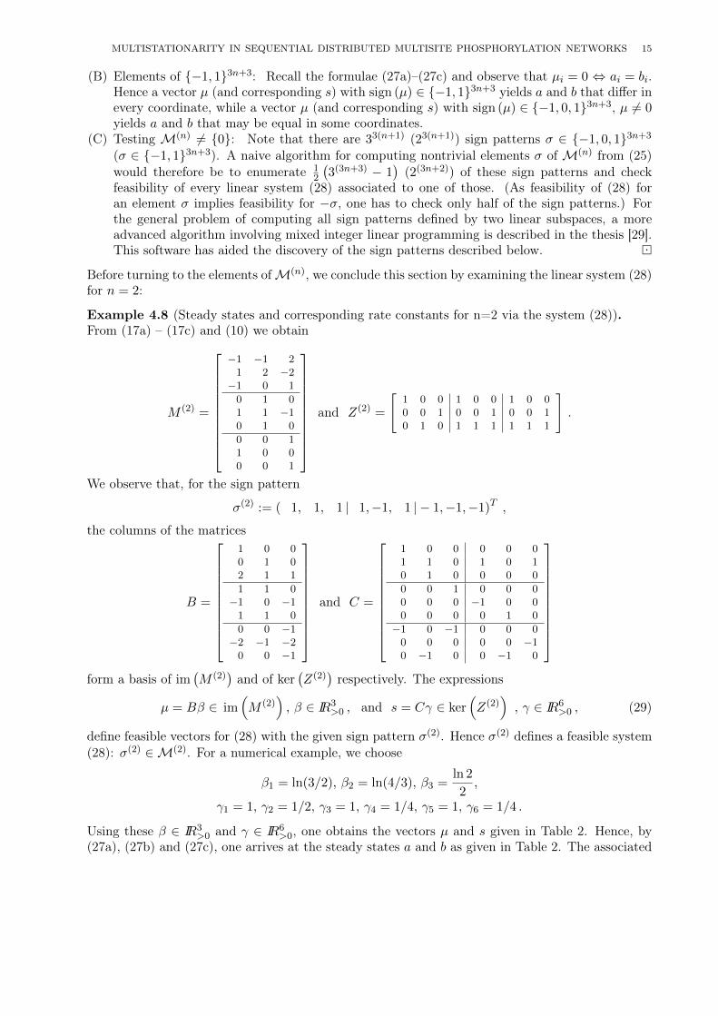
Example 4.8 (Steady states and corresponding rate constants for n=2 via the system (28)).From (17a) – (17c) and (10) we obtain
M (2) =
−1 −1 21 2 −2
−1 0 1
0 1 01 1 −10 1 0
0 0 11 0 00 0 1
and Z(2) =
[1 0 0 1 0 0 1 0 00 0 1 0 0 1 0 0 10 1 0 1 1 1 1 1 1
].
We observe that, for the sign pattern
σ(2) := ( 1, 1, 1 | 1,−1, 1 | − 1,−1,−1)T ,
the columns of the matrices
B =
1 0 00 1 02 1 1
1 1 0−1 0 −11 1 0
0 0 −1−2 −1 −20 0 −1
and C =
1 0 0 0 0 01 1 0 1 0 10 1 0 0 0 0
0 0 1 0 0 00 0 0 −1 0 00 0 0 0 1 0
−1 0 −1 0 0 00 0 0 0 0 −10 −1 0 0 −1 0
form a basis of im
(M (2)
)and of ker
(Z(2)
)respectively. The expressions
µ = Bβ ∈ im(M (2)
), β ∈ IR3
>0 , and s = Cγ ∈ ker(Z(2)
), γ ∈ IR6
>0 , (29)
define feasible vectors for (28) with the given sign pattern σ(2). Hence σ(2) defines a feasible system(28): σ(2) ∈M(2). For a numerical example, we choose
β1 = ln(3/2), β2 = ln(4/3), β3 =ln 2
2,
γ1 = 1, γ2 = 1/2, γ3 = 1, γ4 = 1/4, γ5 = 1, γ6 = 1/4 .
Using these β ∈ IR3>0 and γ ∈ IR6
>0, one obtains the vectors µ and s given in Table 2. Hence, by(27a), (27b) and (27c), one arrives at the steady states a and b as given in Table 2. The associated
16 KATHARINA HOLSTEIN, DIETRICH FLOCKERZI AND CARSTEN CONRADI
µ s a b
ln 32 1 2 3
ln 43 2 6 8
− ln 22 + ln 6 1
2134
(1 + 3
√2)
334
(6 +√
2)
ln 2 1 1 2
ln√23 −1
4328
(3 +√
2)
128
(2 + 3
√2)
ln 2 1 1 2
− ln 22 −2 2
(2 +√
2)
2(1 +√
2)
− ln 6 −14
310
120
− ln 22 −3
2 3 + 3√2
32
(1 +√
2)
Table 2. Columns 1&2: vectors µ and s with sign (µ) = sign (s) satisfying thesystem (28) (with n = 2 and σ(2)). Columns 3&4: Steady state vectors a andb computed from µ and s via (27a), (27b) & (27c). Simple computation showsc = Z(2) a = Z(2) b =
(7 + 2
√2, 1
34
(137 + 54
√2), 1140
(2187 + 505
√2))T .
k1 k2 k3 l1 l2 l3 k4 k5 k6 l4 l5 l65√
2 30√
2 30√
2 952 27 30√
2 43
(4 +√
2)
12
12
403
(4 + 5
√2)
23
23
Table 3. One choice of rate constants such that a and b from Table 2 are steadystates (i.e. κ = (k1, k2, k3, l1, l2, l3, k4, k5, k6, l4, l5, l6)T with S(2) r(2) (κ, a) =
S(2) r(2) (κ, b) = 0).
rate constant vectors κ are obtained by (21c) for the value of a from Table 2 and for free λ ∈ IR6>0.
Here we choose
λ =(
30√
2, 27, 30√
2, 2 +√
2, 2 +√
2, 2 +√
2)T
to obtain the rate constants given in Table 3. For the illustration in Fig. 4, a numerical continuationof the steady state a has been performed using the rate constants from Table 3. The numericalcontinuation reveals that, for the rate constants of Table 3 and the total concentrations c = Z(2)a =Z(2)b defined by either a or b, the system has three steady states, namely a, b and
b = (1.52.., 1.01.., 0.01.., 0.12.., 0.74.., 0.12.., 8.17.., 4.39.., 6.13.. )T .
A local stability analysis shows the exponential stability of b and b. The steady state a turns outto be a saddle point because of the presence of exactly one simple positive eigenvalue. Hence thesystem shows bistability as indicated in Figure 3. By the results of [30], these are all steady statesof the double phosphorylation system once β, γ and λ are fixed. �
4.2. Sign patterns for feasibility of system (28). Given a σ(n) ∈ {−1, 1}3n+3, we first turn tothe subproblem Z(n) s = 0 with sign (s) = σ(n) in (28). To this end, we consider sign patterns in col-umn and matrix form. With (n+1) column vectors τ(0) = (τ10, τ20, τ30)
T , . . . , τ(n) = (τ1n, τ2n, τ3n)T
from {−1, 1}3 we associate the sign pattern matrix
τ =(τ(0) · · · τ(n)
)∈ {−1, 1}3×(n+1) . (30)
and the sign pattern column τ (n) = col(τ) = col(τ(0), ..., τ(n)) ∈ {−1, 1}3n+3.

MULTISTATIONARITY IN SEQUENTIAL DISTRIBUTED MULTISITE PHOSPHORYLATION NETWORKS 17
9.2 9.3 9.4 9.5 9.6 9.7 9.8 9.9 10 10.10
0.5
1
1.5
2
2.5
3
c1
x8
a8 =3
10
b8 =1
20LP
LP
c1 = 7+ 2√
2
Figure 4. Numerical continuation starting in a from Table 3. Here x8 (i.e. theconcentration of A2P ) is plotted against c1 (i.e. the total concentration of kinaseE1). Green triangles mark the components a8 and b8 of the steady state vectors aand b from Table 2, the total concentration c1 at a (and b) is displayed in red. Thecomponent b8 of the third steady state is close to 4.39.
Lemma 4.9 ( Feasibility of Z(n) s = 0 and sign (s) = σ(n) ∈ {−1, 1}3n+3).For a given sign pattern matrix
σ = (σ(0), ..., σ(n)) =
σ10 ... σ1nσ20 ... σ2nσ30 ... σ3n
∈ {−1, 1}3×(n+1)
and its associated sign pattern vector σ(n) = col(σ(0), ..., σ(n)) ∈ {−1, 1}3n+3, the subproblem
Z(n) s = 0 with sign (s) = σ(n) (31)
in (28) is not feasible if and only if σ has one of the following three properties:(1) The elements of the first row are all of the same sign σ10.(2) The elements of the second row are all of the same sign σ20 with σ20σ10 < 0 and σ20σ30 < 0.(3) The elements of the third row are all of the same sign σ30.
Proof. In analogy to σ(n), we use the notation s = (s10, s20, s30, s11, s21, s31, ...... , s1n, s2n, s3n)T .The claim follows easily from the fact that Z(n) s = 0 is equivalent to the decoupled linear system
n∑j=0
s1j = 0,
n∑j=0
s3j = 0,
n∑j=0
s2j = s10 + s30
(cf. the definition of Z(n) in eq.(10)). �
We now turn to those sign patterns σ(n) ∈ {−1, 1}3n+3, where (31) is feasible and where, additionally,the second subproblem
µ = M (n) ξ with sign (µ) = σ(n) (32)is feasible. In particular, we will show that (31) and (32) are only feasible for sign patterns involving
σ1 := (+1,+1,+1)T , σ2 := (+1,−1,+1)T , σ3 := (−1,−1,−1)T = −σ1 (33a)
σ4 := (+1,−1,−1)T , σ5 := (−1,+1,−1)T = −σ2 , σ6 := (−1,+1,+1)T = −σ4, (33b)

18 KATHARINA HOLSTEIN, DIETRICH FLOCKERZI AND CARSTEN CONRADI
while it is infeasible for sign patterns involving
σ7 := (+1,+1,−1)T , σ8 := (−1,−1,+1)T = −σ7. (33c)
We use these σj to encode sign patterns σ(n) ∈ {−1, 1}3n+3. For example, for n = 2 we encode
σ(2) := ( 1, 1, 1| 1,−1, 1| − 1,−1,−1)T ∈ IR9 (34)
as the 3× 3 arrayσ = (σ1 σ2 σ3)
with the columns σ1, σ2 and σ3. We use the symbol [τ ]i as shorthand notation for the i-foldconcatenation of τ ∈ {−1, 1}3, i.e., for the 3× i–matrix
[τ ]i = ( τ . . . τ︸ ︷︷ ︸i times
) . (35)
For an example with n = 5,
σ = ([σ3]3 [σ5]2 σ1) = (σ3σ3σ3σ5σ5σ1)
stands for the 18-dimensional sign pattern
σ(5) = (−1,−1,−1| − 1,−1,−1| − 1,−1,−1| − 1,+1,−1| − 1,+1,−1|+ 1,+1,+1)T .
In the following Theorem 4.10 we characterize the sign patterns σ(n) ∈ {−1, 1}3n+3 that are feasiblefor (28) for n ≥ 2. In Section 6 below we will prove this result.
Theorem 4.10. Recall the linear system (28) associated to the sign pattern vector σ(n) ∈ {−1, 1}3n+3
and hence to the equivalent sign pattern matrix σ ∈ {−1, 1}3×(n+1). For n ≥ 2 the linear systems(28) associated to σ(n) and to −σ(n) are feasible if and only if σ is one of the following sign patterns(s1) to (s7):
• For n ≥ 2:
σ =(σ2 [σ3]i1 [σ1]i2
)with i1, i2 ≥ 1 and i1 + i2 = n (s1)
σ =(σ3 [σ5]i1 [σ1]i2
)with i1, i2 ≥ 1 and i1 + i2 = n (s2)
σ =(σ4 [σ5]i1 [σ1]i2
)with i1 = 1, i2 ≥ 1 and i1 + i2 = n (s3)
σ =(σ4 [σ3]i1 [σ1]i2
)with i1, i2 ≥ 1 and i1 + i2 = n . (s4)
• Additionally for n ≥ 3:
σ =(σ2 [σ3]i1 [σ2]i2 [σ1]i3
)with i1, i2, i3 ≥ 1 and i1 + i2 + i3 = n (s5)
σ =(σ3 [σ3]i1 [σ5]i2 [σ1]i3
)with i1, i2, i3 ≥ 1 and i1 + i2 + i3 = n (s6)
σ =(σ4 [σ3]i1 [σ5]i2 [σ1]i3
)with i1 , i3 ≥ 1, i2 = 1 and i1 + i2 + i3 = n . (s7)
By Remark 4.7(A), σ(n) is a nontrivial element ofM(n) from (25) if and only if σ(n) is one of thesign patterns (s1) to (s7) or its negative. As an immediate consequence of Theorem 4.10 above wenote the following:
Remark 4.11 (M (n) 6= {0}: multistationarity in n-site sequential distributive phosphorylation forn ≥ 2).As a consequence of Theorem 4.6 and 4.10 we conclude that for every n ≥ 2 there exists a vectorof rate constants κ such that the system (14a), (14b) & (14c) has at least two distinct positivesolutions a and b. Every element σ described in Theorem 4.10 defines a feasible linear system ofthe form (28). And solutions thereof parameterize the steady states a and b and the vectors κ ofrate constants via the equations (27a), (27b) and (21c) respectively (cf. Example 4.8). It will beinteresting to systematically explore the corresponding regions in the rate constant space, especiallywith respect to biological plausibility and function.

MULTISTATIONARITY IN SEQUENTIAL DISTRIBUTED MULTISITE PHOSPHORYLATION NETWORKS 19
Remark 4.12 (M(1) = {0} excludes multistationarity for n = 1 (single phosphorylation)).Any µ ∈ im
(M (1)
)and any s ∈ ker
(Z(1)
)can be written as
µ = (µ1, µ4 − µ1, µ3, µ4, µ4 − µ1, µ4)T and s = (s1, s2, s3,−s1, s3 − s2 + s1,−s3)T
respectively. We assume sign(µ) = sign(s). In case of µ4 = 0 we arrive at µ = 0 = s. Incase of µ4 6= 0 we assume without loss of generality µ4 > 0 and are led to the sign patternσ(1) = (−,+,−,+,+,+)T with sign pattern matrix
σ =
− ++ +− +
.
By Lemma 4.9 these sign patterns cannot belong to an element of ker(Z(1)
)and we conclude
M(1) = {0}.
Finally we want to count the number of sign patterns of the form (s1) – (s7). To demonstrate thereasoning we first examine sign patterns of the form (s2) for n = 2, . . . , 5:
Example 4.13 (The sign pattern (s2)).For 2 ≤ n ≤ 5 one obtains from the formula (s2) the following patterns:
n = 2 n = 3 n = 4 n = 5
σ3 σ5 σ1σ3 σ5 σ5 σ1
σ3 σ5 σ1 σ1
σ3 σ5 σ5 σ5 σ1
σ3 σ5 σ5 σ1 σ1
σ3 σ5 σ1 σ1 σ1
σ3 σ5 σ5 σ5 σ5 σ1
σ3 σ5 σ5 σ5 σ1 σ1
σ3 σ5 σ5 σ1 σ1 σ1
σ3 σ5 σ1 σ1 σ1 σ1
We summarize for (s2) in case of n = 5:• The integer 5 can be partitioned in the sum of two integers i1, i2 in the following two ways:
5 = 1 + 4 = 3 + 2. As we have to take the ordering of i1 and i2 into account (and hence, forexample, (4, 1) differs from (1, 4)) we obtain the following pairs of integers:
{(1, 4) , (4, 1) , (3, 2) , (2, 3)} .
• This yields the sign patterns
σ3 [σ5]4 [σ1]1 , σ3 [σ5]1 [σ1]4 , σ3 [σ5]3 [σ1]2 , σ3 [σ5]2 [σ1]3
�
Concerning the number of elements σ(n) ∈ {−1, 1}3n+3 corresponding to (s1) – (s7) we observe
Proposition 4.14.For n ≥ 3 there exist (n− 1)(n+ 2) elements in {−1, 1}3×(n+1) of the form (s1) – (s7).
Proof. We note that for n ≥ 3 fixed formulae (s5) and (s6) each yield as many elements as thereare partitions of n into three positive integers (taking order into account). Similarly (s1), (s2) and(s4) each yield as many elements as there are partitions of n into two positive integers (taking orderinto account), while (s7) yields as many elements as there are partitions of n− 1 into two positiveintegers (taking order into account). Finally, (s3) yields one element.First we count the number of ways an integer can be partitioned into the sum of two positive integers(if order is taken into account). One has
n = (n− 1) + 1 = (n− 2) + 2 = · · · = (n− (n− 1)) + (n− 1) .
20 KATHARINA HOLSTEIN, DIETRICH FLOCKERZI AND CARSTEN CONRADI
Note that there is no other way to partition n into the sum of two positive integers. Hence weconclude that there is a total of n− 1 ways to partition n into two positive integers.Second we count the number of partitions of n into three positive integers. To this end we observe:
n = (n− 2) + (1 + 1)
= (n− 3) + {2 ways to write 3 as the sum of two positive integers}...= (n− j) + {j − 1 ways to write j as the sum of two positive integers}...= (n− (n− 1)) + {n− 2 ways to write n− 1 as the sum of two positive integers}
Consequently there is a total of
n−1∑j=2
(j − 1) =1
2(n− 2) (n− 1)
ways to partition n into the sum of three positive integers. Now we can sum over the contributionof each of the formulae
(n− 2)(n− 1)︸ ︷︷ ︸(s5) & (s6)
+ 3 (n− 1)︸ ︷︷ ︸(s1), (s2) & (s4)
+ (n− 2)︸ ︷︷ ︸(s7)
+ ( 1 )︸ ︷︷ ︸(s3)
= (n− 1)(n+ 2) .
�
5. Proof of Theorem 4.2
To prove the Theorem 4.2 we show the following implications:
(A)⇒ (D)⇒ (C)⇒ (B)⇒ (A)
(A)⇒ (D) :
Suppose there exists a, b ∈ IR3n+3>0 and κ ∈ IR3n+3
>0 such that (14a) & (14b) hold. Then, byTheorem 4.3 of [20] one has
ln b− ln a ∈ im(AT),
with
A =
1 0 0 1 1 1 2 2 2 . . . n n n1 0 1 1 0 1 1 0 1 . . . 1 0 10 1 0 1 1 1 1 1 1 . . . 1 1 1
,where the columns of A have been reordered to match the ordering introduced in Table 1 (in theaforementioned reference [20], the columns of A correspond to the exponents of t1, t2, t3 in thestatement of Theorem 4.3, the matrix itself is displayed in the proof of said Theorem).
AT = M (n)Q for the nonsingular Q :=
n 0 11 1 12 1 1
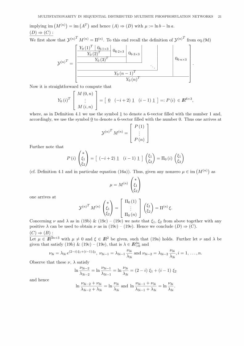
MULTISTATIONARITY IN SEQUENTIAL DISTRIBUTED MULTISITE PHOSPHORYLATION NETWORKS 21
implying im(M (n)
)= im
(AT)and hence (A)⇒ (D) with µ := ln b− ln a.
(D)⇒ (C) :
We first show that Y(n)T M (n) = Π(n). To this end recall the definition of Y(n)T from eq.(9d)
Y(n)T =
Y0 (1)T 06·1×3 06·2×3 06·3×306·n×3
Y0 (2)T
Y0 (3)T
. . .Y0 (n− 1)T
Y0 (n)T
.
Now it is straightforward to compute that
Y0 (i)T
M (0, n)...
M (i, n)
=[
0 (−i+ 2) 1 (i− 1) 1]
=: P (i) ∈ IR6×3,
where, as in Definition 4.1 we use the symbol 1 to denote a 6-vector filled with the number 1 and,accordingly, we use the symbol 0 to denote a 6-vector filled with the number 0. Thus one arrives at
Y(n)T M (n) =
P (1)...
P (n)
Further note that
P (i)
∗ξ1ξ2
=[
(−i+ 2) 1 (i− 1) 1] (ξ1
ξ2
)= Π0 (i)
(ξ1ξ2
)(cf. Definition 4.1 and in particular equation (16a)). Thus, given any nonzero µ ∈ im
(M (n)
)as
µ = M (n)
∗ξ1ξ2
one arrives at
Y(n)T M (n)
∗ξ1ξ2
=
Π0 (1)...
Π0 (n)
(ξ1ξ2)
= Π(n) ξ.
Concerning ν and λ as in (19b) & (19c) – (19e) we note that ξ1, ξ2 from above together with anypositive λ can be used to obtain ν as in (19c) – (19e). Hence we conclude (D)⇒ (C).(C)⇒ (B) :
Let µ ∈ IR3n+3 with µ 6= 0 and ξ ∈ IR2 be given, such that (19a) holds. Further let ν and λ begiven that satisfy (19b) & (19c) – (19e), that is λ ∈ IR3n
>0 and
ν3i = λ3i e(2−i) ξ1+(i−1) ξ2 , ν3i−1 = λ3i−1
ν3iλ3i
and ν3i−2 = λ3i−2ν3iλ3i
, i = 1, . . . , n.
Observe that these ν, λ satisfy
lnν3i−2λ3i−2
= lnν3i−1λ3i−1
= lnν3iλ3i
= (2− i) ξ1 + (i− 1) ξ2
and hencelnν3i−2 + ν3iλ3i−2 + λ3i
= lnν3iλ3i
and lnν3i−1 + ν3iλ3i−1 + λ3i
= lnν3iλ3i
.
22 KATHARINA HOLSTEIN, DIETRICH FLOCKERZI AND CARSTEN CONRADI
Defineν(i) := (ν3i−2, ν3i−1, ν3i) and λ(i) := (λ3i−2, λ3i−1, λ3i)
and letν = col
(ν(1), . . . , ν(n)
)and col
(λ(1), . . . , λ(n)
).
Recall the matrices E(n) and E from eqns. (15b) & (15a) and observe that
lnE(n) ν
E(n) λ=
(lnE ν(1)
E λ(1), . . . , ln
E ν(n)
E λ(n)
)and
lnE ν(i)
E λ(i)=
(lnν3i−2 + ν3iλ3i−2 + λ3i
, lnν3i−2λ3i2
, lnν3iλ3i
, lnν3i−1 + ν3iλ3i−1 + λ3i
, lnν3i−1λ3i−1
, lnν3iλ3i
).
Hence one has for ν, λ from above
lnE ν(i)
E λ(i)=[
(2− i) 1 (i− 1) 1](ξ1
ξ2
)and
lnE(n) ν
E(n) λ= Π(n) ξ.
Consequently, if there exist vectors µ ∈ IR3n+3, µ 6= 0 and ξ ∈ IR2 satisfying (19a) and vectors ν, λsatisfying (19b), (19c) – (19e), then µ, ν and λ also satisfy (18). Note that ν and λ satisfying (19b)& (19c) – (19e) are positive. Thus we conclude (C)⇒ (B).(B)⇒ (A) :
Finally, assume µ ∈ IR3n+3 with µ 6= 0 and (ν, λ) ∈ IR3n>0 × IR3n
>0 satisfy (18). Fix a ∈ IRn>0 anddefine
b := diag (eµ) a
κ := diag(
Φ(n)(a−1))
E(n) λ.
Then
S(n) diag (κ) Φ(n) (a) = S(n) diag(
Φ(n)(a−1))
diag(E(n) λ
)Φ(n) (a) = S(n)E(n) λ = 0
and (as, by (18), Y(n)T µ = ln E(n) νE(n) λ
)
S(n) diag (κ) Φ(n) (b) = S(n) diag (κ) diag(
Φ(n) (a))eY
(n)T µ = S(n)E(n) ν = 0
and therefore (B)⇒ (A) where we have used equation (13a) of Remark 3.4. �
6. Proof of Theorem 4.10
First, we observe that sign(M (n) ξ
)= σ(n) implies sign
(M (n) (−ξ)
)= −σ(n) and that Z(n) s = 0
implies Z(n) (−s) = 0. Hence, if the system (28) associated to σ(n) is feasible for (ξ, s), then thesystem (28) associated to −σ(n) is feasible for (−ξ, −s). Thus σ(n) ∈ M(n) implies −σ(n) ∈ M(n).
MULTISTATIONARITY IN SEQUENTIAL DISTRIBUTED MULTISITE PHOSPHORYLATION NETWORKS 23
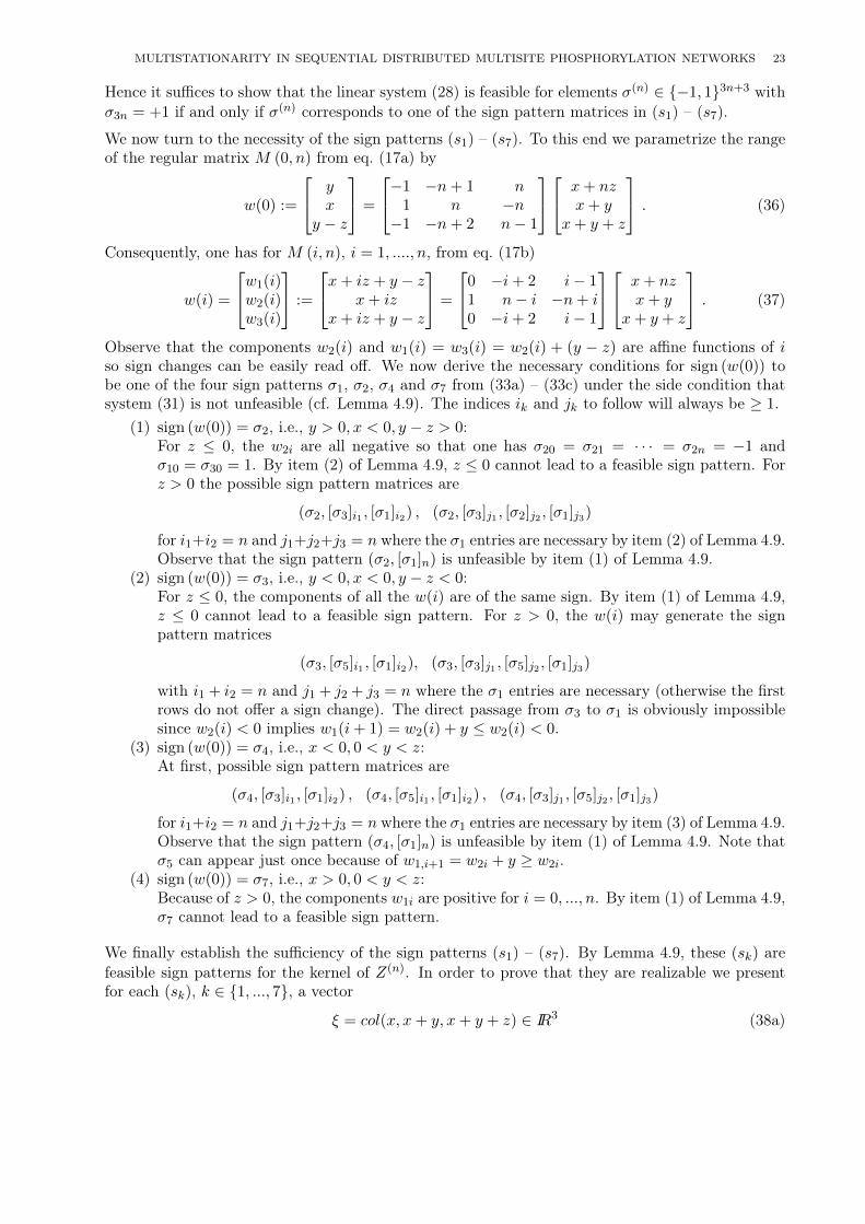
Hence it suffices to show that the linear system (28) is feasible for elements σ(n) ∈ {−1, 1}3n+3 withσ3n = +1 if and only if σ(n) corresponds to one of the sign pattern matrices in (s1) – (s7).
We now turn to the necessity of the sign patterns (s1) – (s7). To this end we parametrize the rangeof the regular matrix M (0, n) from eq. (17a) by
w(0) :=
yx
y − z
=
−1 −n+ 1 n1 n −n−1 −n+ 2 n− 1
x+ nzx+ y
x+ y + z
. (36)
Consequently, one has for M (i, n), i = 1, ...., n, from eq. (17b)
w(i) =
w1(i)w2(i)w3(i)
:=
x+ iz + y − zx+ iz
x+ iz + y − z
=
0 −i+ 2 i− 11 n− i −n+ i0 −i+ 2 i− 1
x+ nzx+ y
x+ y + z
. (37)
Observe that the components w2(i) and w1(i) = w3(i) = w2(i) + (y − z) are affine functions of iso sign changes can be easily read off. We now derive the necessary conditions for sign (w(0)) tobe one of the four sign patterns σ1, σ2, σ4 and σ7 from (33a) – (33c) under the side condition thatsystem (31) is not unfeasible (cf. Lemma 4.9). The indices ik and jk to follow will always be ≥ 1.
(1) sign (w(0)) = σ2, i.e., y > 0, x < 0, y − z > 0:For z ≤ 0, the w2i are all negative so that one has σ20 = σ21 = · · · = σ2n = −1 andσ10 = σ30 = 1. By item (2) of Lemma 4.9, z ≤ 0 cannot lead to a feasible sign pattern. Forz > 0 the possible sign pattern matrices are
(σ2, [σ3]i1 , [σ1]i2) , (σ2, [σ3]j1 , [σ2]j2 , [σ1]j3)
for i1+i2 = n and j1+j2+j3 = n where the σ1 entries are necessary by item (2) of Lemma 4.9.Observe that the sign pattern (σ2, [σ1]n) is unfeasible by item (1) of Lemma 4.9.
(2) sign (w(0)) = σ3, i.e., y < 0, x < 0, y − z < 0:For z ≤ 0, the components of all the w(i) are of the same sign. By item (1) of Lemma 4.9,z ≤ 0 cannot lead to a feasible sign pattern. For z > 0, the w(i) may generate the signpattern matrices
(σ3, [σ5]i1 , [σ1]i2), (σ3, [σ3]j1 , [σ5]j2 , [σ1]j3)
with i1 + i2 = n and j1 + j2 + j3 = n where the σ1 entries are necessary (otherwise the firstrows do not offer a sign change). The direct passage from σ3 to σ1 is obviously impossiblesince w2(i) < 0 implies w1(i+ 1) = w2(i) + y ≤ w2(i) < 0.
(3) sign (w(0)) = σ4, i.e., x < 0, 0 < y < z:At first, possible sign pattern matrices are
(σ4, [σ3]i1 , [σ1]i2) , (σ4, [σ5]i1 , [σ1]i2) , (σ4, [σ3]j1 , [σ5]j2 , [σ1]j3)
for i1+i2 = n and j1+j2+j3 = n where the σ1 entries are necessary by item (3) of Lemma 4.9.Observe that the sign pattern (σ4, [σ1]n) is unfeasible by item (1) of Lemma 4.9. Note thatσ5 can appear just once because of w1,i+1 = w2i + y ≥ w2i.
(4) sign (w(0)) = σ7, i.e., x > 0, 0 < y < z:Because of z > 0, the components w1i are positive for i = 0, ..., n. By item (1) of Lemma 4.9,σ7 cannot lead to a feasible sign pattern.
We finally establish the sufficiency of the sign patterns (s1) – (s7). By Lemma 4.9, these (sk) arefeasible sign patterns for the kernel of Z(n). In order to prove that they are realizable we presentfor each (sk), k ∈ {1, ..., 7}, a vector
ξ = col(x, x+ y, x+ y + z) ∈ IR3 (38a)

24 KATHARINA HOLSTEIN, DIETRICH FLOCKERZI AND CARSTEN CONRADI
leading to the sign pattern (sk) for M (n)ξ:
For (s1): x = i2 − 34 , y = −n+ 5
4 , z = 1 .
For (s2): x = n− 14 , y = −n− i1 + 3
4 , z = 1 .
For (s3): x = n− 34 , y = −n+ 1
4 , z = 1 .
For (s4): x = i2 − 14 , y = −n+ 3
4 , z = 1 .
For (s5): x = i3 − 34 , y = −n+ i2 + 5
4 , z = 1 .
For (s6): x = i2 + i3 − 14 , y = −n− i2 + 3
4 , z = 1 .
For (s7): x = i2 + 14 , y = −n+ 1
4 , z = 1 .
(38b)
�
7. Discussion
The main topic of this contribution is the existence of multistationarity for n-site sequential distribu-tive phosphorylation. Via the equations (21c) and (27a) – (27c) we were able to link the existence ofpairs of steady states (a, b) and a corresponding vector of rate constants κ to solutions of the linearsystems (28). These systems are uniquely defined by sign patterns σ(n) ∈ {−1, 0, 1}3n+3 and hencethe existence of a single sign pattern defining a feasible system (28) is sufficient. Concerning signpatterns σ ∈ {−1, 1}3n+3 where (28) is feasible, Theorem 4.10 establishes four such sign patternsfor n = 2 and (n− 1) (n+ 2) for n ≥ 3.Unfortunately the biological interpretation of elements σ where (28) is feasible is unclear (unlike inthe case of multistationarity itself, that is usually associated with a specific biological function). Ifdifferent elements could be associated to different biological functions, this would limit the number of(different) biological functions a network can perform and hence be of significant biological interest.Moreover, knowledge of all sign patterns σ defining feasible (28) would then correspond to knowledgeof all biological functions a network is capable of.However, the following observations concerning pairs of steady states (a, b) can easily be madeby inspection of the feasible sign patterns (s1) – (s7) and the structure of the matrices M (i) from(17b): (i) every sign pattern ends with the triplet (1, 1, 1)T or (−1,−1,−1)T and hence the lastthree components of steady state b are greater (smaller) than those of a (recall that µ = ln bi
aiand
hence µi > 0 implies bi > ai and µi < 0 implies bi < ai). (ii) The first and the third row of thematrices M (i) are identical. Hence µ3i+1 = µ3i+3, i = 1, . . . , n. For a pair of steady states (a, b)these correspond to the ratio of steady state concentrations of kinase-substrate complex Ai−1 pE1 (incase of µ3i+1) and phosphatase-substrate complex Aip E2 (in case of µ3i+3, cf. Table 1). Hence, forany pair of steady states, the ratio of the steady state concentrations of kinase-substrate complexesequals that of phosphatase-substrate complexes.Finally we’d like to discuss two observations related to the formulae (21c) and (27a) – (27c). Considera sign pattern matrix σ as in (s1) – (s7) and let σ(n) be the corresponding sign pattern vector. Pickvectors µ ∈ im
(M (n)
), s ∈ im
(S(n)
)with sign (s) = sign (µ) = σ(n). Let (aσ, bσ) be the pair of
steady states defined by µ, s via (27a) – (27c). Let (a−σ, b−σ) be the pair of steady states definedby −µ and −s. Then it is not difficult to see that a−σ = bσ and b−σ = aσ (cf. a similar discussionin [4]). Further note that a given pair (a, b), obtained via (27a) – (27c), is a pair of steady statesfor all vectors of rate constants defined by the formula (21c), where λ ∈ IR3n
>0 is free.The formula (21c) for the vectors of rate constants may be interesting for two reasons: first, itallows to replace the 6n rate constants ki, li by the 3n ‘coordinates’ λi and hence a reduction ofthe degrees of freedom in the dynamical system (12). Second, it means that multistationarity isrobust with respect to perturbations within the image of the map (21c) and fragile with respect totransversal perturbations. In a future publication we will explore the image of this map with theaim of establishing parameter values for multistationarity in biologically meaningful domains.

MULTISTATIONARITY IN SEQUENTIAL DISTRIBUTED MULTISITE PHOSPHORYLATION NETWORKS 25
7.1. Acknowledgments. KH and CC acknowledge financial support from the International MaxPlanck Research School in Magdeburg and the Research Center ’Dynamic Systems’ of the Ministryof Education of Saxony-Anhalt, respectively. Finally, we’d like to thank the diligent reviewers fortheir valuable suggestions.
References
[1] D. Barik, W. T. Baumann, M. R. Paul, B. Novak, and J. J. Tyson. A model of yeast cell-cycle regulation basedon multisite phosphorylation. Molecular Systems Biology, 6:1–18, 2010.
[2] K. C. Chen, L. Calzone, A. Csikasz-Nagy, F. R. Cross, B. Novak, and J. J. Tyson. Integrative analysis of cellcycle control in budding yeast. Molecular Biology of the Cell, 15(8):3841–3862, 2004.
[3] C. Conradi and D. Flockerzi. Multistationarity in mass action networks with applications to ERK activation.Journal of Mathematical Biology, 65(1):107–156, 2012.
[4] C. Conradi, D. Flockerzi, and J. Raisch. Multistationarity in the activation of a MAPK: Parametrizing therelevant region in parameter space. Mathematical Biosciences, 211:05–131, 2008.
[5] C. Conradi, J. Saez-Rodriguez, E.-D. Gilles, and J. Raisch. Using chemical reaction network theory to discarda kinetic mechanism hypothesis. Systems Biology, IEE Proceedings (now IET Systems Biology), 152(4):243–248,2005.
[6] C. Conradi, J. Saez-Rodriguez, E.-D. Gilles, and J. Raisch. Chemical Reaction Network Theory – a tool forsystems biology. Proceedings of the 5th MATHMOD, 2006.
[7] M. T. Cooling, P. Hunter, and E. J. Crampin. Sensitivity of NFAT cycling to cytosolic calcium concentration:implications for hypertrophic signals in cardiac myocytes. Biophysical Journal, 96:2095–2104, 2009.
[8] G. R. Crabtree and E. N. Olson. NFAT signaling: Choreographing the social lives of cells. Cell, 109(2, Supplement1):S67–S79, 2002.
[9] M. Feinberg. The existence and uniqueness of steady states for a class of chemical reaction networks. Archivefor Rational Mechanics and Analysis, 132:311–370, 1995.
[10] M. Feinberg. Multiple steady states for chemical reaction networks of deficiency one. Archive for Rational Me-chanics and Analysis, 132:371–406, 1995.
[11] E. Feliu and C. Wiuf. Enzyme-sharing as a cause of multi-stationarity in signalling systems. Journal of TheRoyal Society Interface, 9(71):1224–1232, 2012.
[12] J. Gunawardena. Multisite protein phosphorylation makes a good threshold but can be a poor switch. Proceedingsof the National Academy of Sciences, 102(41):14617–14622, 2005.
[13] J. Gunawardena. Distributivity and processivity in multisite phosphorylation can be distinguished throughsteady-state invariants. Biophysical Journal, 93(11):3828–3834, 2007.
[14] N. Hermann-Kleiter and G. Baier. NFAT pulls the strings during CD4+ T helper cell effector functions. Blood,115(15):2989–2997, 2010.
[15] K. Holstein, D. Flockerzi, and C. Conradi. Parameter regimes for bistability in multisite phosphorylation net-works. in preparation, 2013.
[16] C.-Y. F. Huang and J. E. Ferrell. Ultrasensitivity in the mitogen-activated protein kinase cascade. Proceedingsof the National Academy of Science, 93(19):10078–10083, 1996.
[17] S. Klamt and J. Gagneur. Computation of elementary modes: a unifying framework and the new binary approach.BMC Bioninformatics, 175(5), 2004.
[18] F. Macian. NFAT proteins: key regulators of T-cell development and function. Nature Reviews Immunology,5(6):472–484, 2005.
[19] N. I. Markevich, J. B. Hoek, and B. N. Kholodenko. Signaling switches and bistability arising from multisitephosphorylation in protein kinase cascades. Journal of Cell Biology, 164(3):353–359, 2004.
[20] M. Pérez Millán, A. Dickenstein, A. Shiu, and C. Conradi. Chemical reaction systems with toric steady states.Bulletin of Mathematical Biology, 74:1027–1065, 2012.
[21] C. Salazar and T. Höfer. Versatile regulation of multisite protein phosphorylation by order of phosphate pro-cessing and protein-protein interactions. Federation of European Biochemical Societies, 274:1046–1061, 2007.
[22] C. Salazar and T. Höfer. Multisite protein phosphorylation – from molecular mechanisms to kinetic models.FEBS Journal, 276(12):3177–3198, 2009.
[23] R. Seger and E. G. Krebs. The MAPK signaling cascade. The FASEB Journal, 9:726–735, 1995.[24] Y. D. Shaul and R. Seger. The MEK/ERK cascade: From signaling specificity to diverse functions. Biochimica
et Biophysica Acta (BBA) – Molecular Cell Research, 1773(8):1213–1226, 2007.[25] M. Thomson and J. Gunawardena. The rational parameterisation theorem for multisite post-translational mod-
ification systems. Journal of Theoretical Biology, 261(4):626–636, 2009.[26] M. Thomson and J. Gunawardena. Unlimited multistability in multisite phosphorylation systems. Nature,
460(7252):274–277, 2009.

26 KATHARINA HOLSTEIN, DIETRICH FLOCKERZI AND CARSTEN CONRADI
[27] T. Tomida, K. Hirose, A. Takizawa, F. Shibasaki, and M. Iino. NFAT functions as a working memory of Ca+2
signals in decoding Ca+2 oscillation. The European Molecular Biology Organization Journal, 22(15):3825–3832,2003.
[28] J. J. Tyson and B. Novák. Temporal organization of the cell cycle. Current Biology, 18:R759–R768, 2008.[29] M. Uhr. Structural analysis of inference problems arising in systems biology. PhD thesis, ETH Zurich, 2012.[30] L. Wang and E. Sontag. On the number of steady states in a multiple futile cycle. Journal of Mathematical
Biology, 57:29–52, 2008.[31] Z. Yao and R. Seger. The ERK signaling cascade – views from different subcellular compartments. BioFactors,
35(5):407–416, 2009.
Max-Planck-Institut Dynamik komplexer technischer Systeme, Sandtorstr. 1, 39106 Magdeburg,Germany.E-mail address: [email protected],[email protected],[email protected]


![Multisite Phosphorylation Provides an Effective and ...cheresearch.engin.umich.edu/lin/publications/... · multisite phosphorylation [9,32,40–44], and substrate competition [45]](https://img.dokumen.tips/doc/110x75/5fbc6296dcda681bbd3afe99/multisite-phosphorylation-provides-an-effective-and-multisite-phosphorylation.jpg)