Multisource Least-squares Reverse Time Migration Wei Dai

Multisource Least-squares Reverse Time Migration

Wei Dai

Outline• Introduction and Overview

• Chapter 2: Multisource least-squares reverse time

migration

• Chapter 3: Frequency-selection encoding LSRTM

• Chapter 4: Super-virtual inteferometric diffractions

• Summary

Introduction: Least-squares Migration

• Seismic migration: Given: Observed data

modelling operator

Goal: find a reflectivity model to explain by solving

the equation

Direct solution: expensive

Conventional migration:

Iterative solution:

Migration velocity

0 X (km) 60 X (km) 6

30

Z (

km)

• Problems in conventional migration image

Introduction: Motivation for LSM

migration artifacts

migration artifacts

imbalanced amplitudeimbalanced amplitude

• Least-squares migration has been shown to

produce high quality images, but it is considered

too expensive for practical imaging.

• Solution: combine multisource technique and

least-squares migration (MLSM).

Problem of LSM

Motivation for MultisourceMotivation for Multisource

Multisource LSMTo: Increase efficiency Remove artifacts Suppress crosstalk

• Problem: LSM is too slow

• Solution: multisource phase-encoding technique• Solution: multisource phase-encoding technique

Many (i.e. 20) times slower than standard migrationMany (i.e. 20) times slower than standard migration

Multisource Migration Image

Multisource CrosstalkMultisource Crosstalk

Overview• Chapter 2 : Multisource least-squares reverse time

migration is implemented with random time-shift and

source-polarity encoding functions.

• Chapter 3: Multisource LSRTM is implemented with

frequency-selection encoding for marine data.

• Chapter 4: An interferometric method is proposed to

extract diffractions from seismic data and enhance its

signal-to-noise ratio.



migration



• Summary

Random Time Shift𝑳𝟏𝒎=𝒅𝟏

O(1/S) cost!

Encoding Matrix

Supergather

Random source time shifts

𝑳𝟐𝒎=𝒅𝟐

𝒅=𝑵𝟏𝒅𝟏+𝑵𝟐𝒅𝟐

Encoded supergather modeler

𝑳𝒎=[𝑵 ¿¿𝟏𝑳𝟏+𝑵𝟐 𝑳𝟐 ]𝒎¿

Random Time Shift𝑳𝟏𝒎=𝒅𝟏

Encoding Matrix

Supergather

𝑳𝟐𝒎=𝒅𝟐

𝒅=𝑵𝟏𝒅𝟏+𝑵𝟐𝒅𝟐

Encoded supergather modeler

𝑳𝒎=[𝑵 ¿¿𝟏𝑳𝟏+𝑵𝟐 𝑳𝟐 ]𝒎¿

× (-1) × (+1)

Conventional Least-squares

Find: an s.t. min

Given: &

Direct solution:

Iterative solution:

Note: subscripts agree

If is too big

In general, hugedimension matrix

Problem: Each prediction is a FD solve

Solution: Multisource technique

Conventional Least-squares

Multisource Least-squares

Find: an s.t. min

Given: &

Direct solution:

In general, smalldimension matrix

If is too big

Iterative solution:

+ crosstalk

0 X (km) 18

0Z

(km

)7.

5

4.5

1.5

km/s

Size: 1800 x 750Grid interval: 10 mSource number: 1800Receiver number: 1800

FD kernel: 2-4 staggered gridSource: 15 Hz

HESS VTI Model

HESS VTI ModelDelta and Epsilon Models

0Z

(km

)7.

5

1.5

0

0 X (km) 18

0Z

(km

)7.

5

2.5

0

Delta

Epsilon

Migration Velocity and Reflectivity

0Z

(km

)7.

5

4.5

1.5

0 X (km) 18

0Z

(km

)7.

5

0.2

-0.4

km/sMigration Velocity

Reflectivity

RTM VS Multisource LSRTM

0 X (km) 18

0Z

(km

)7.

5

0 X (km) 18

0Z

(km

)7.

5

8 supergather30 iterationsSpeedup: 3.75

Standard RTM

Multisource LSRTM, 1 Supergather Multisource LSRTM, 4 Supergather Multisource LSRTM, 8 Supergather

Artifacts removed

Resolution Enhanced

Signal-to-noise Ratio

SNR ∞

3D SEG/EAGE Model400 Shots Evenly Distributed400 Shots Evenly Distributed

Size: 676 x 676 x 201Grid interval: 20 mReceiver: 114244

Source: 5.0 hz

13.5 km

4.0 km 13.5 km

Smooth Migration Velocity

20

13.5 km

4.0 km 13.5 km

Obtained by 3D boxcar smoothingObtained by 3D boxcar smoothing

Conventional RTM

13.5 km

4.0 km13.5 km

400 Shots, Migrated One by One400 Shots, Migrated One by One

13.5 km

4.0 km13.5 km

LSRTM400 Shots, 25 Shots/Supergather400 Shots, 25 Shots/Supergather

13.5 km

4.0 km13.5 km

Conventional RTM100 Shots100 Shots

13.5 km

4.0 km13.5 km

LSRTM100 Shots, 10 Shots/Supergather100 Shots, 10 Shots/Supergather

Chapter 2: Conclusions

• MLSM can produce high quality images efficiently.

LSM produces high quality image.

Multisource technique increases computational

efficiency.

SNR analysis suggests that not too many iterations

are needed.

• Random encoding is not applicable to marine streamer data.

Fixed spread geometry (synthetic) Marine streamer geometry (observed)

6 traces 4 traces

Mismatch between acquisition geometries will dominate the misfit.

Chapter 2: Limitations



migration



• Summary

28

observeddata

simulateddata

misfit = erroneous

misfit

Problem with Marine Data

29

Solution• Every source is encoded with a unique

signature.

observed simulated

• Every receiver acknowledge the contribution from the ‘correct’ sources.

4 shots/group

R( )w

Group 1

Nw frequency bands of source spectrum:

Frequency Selection

2 km

w

Accommodate up to Nw shots

Single Frequency Modeling

(𝜵𝟐+𝝎𝟐

𝒗𝟐 )~𝑷=−𝐖 (𝝎 )𝛅(𝒙 −𝒔)

Helmholtz Equation

(𝜵𝟐−𝟏𝒗𝟐

𝝏𝟐

𝝏𝟐 𝒕 )𝐏=−𝐑𝐞 {𝐖 (𝝎 )𝐞𝐱𝐩 (−𝒊𝝎𝒕)}𝛅(𝒙−𝒔)

Acoustic Wave Equation

• Advantages: Lower complexity in 3D case.

Applicable with multisource technique.

Harmonic wave source

Single Frequency Modeling

(𝜵𝟐−𝟏𝒗𝟐

𝝏𝟐

𝝏𝟐 𝒕 )𝐏=−𝐑𝐞 {𝐖 (𝝎 )𝐞𝐱𝐩 (−𝒊𝝎𝒕)}𝛅(𝒙−𝒔)

Am

plit

ud

e

T T

Single Frequency ModelingA

mp

litu

de

0 Freqency (Hz) 50

Am

plit

ud

e

20 Freqency (Hz) 30

Marmousi2

0 X (km) 8

0Z

(km

)3

.5

4.5

1.5

km/s

• Model size: 8 x 3.5 km• Shots: 301

• Cable: 2km

• Receivers: 201

• Freq.: 400 (0~50 hz)

0 X (km) 8

0Z

(km

)3

.5

0 X (km) 8

Z (

km)

3.5

Conventional RTM0

LSRTM Image (iteration=1)LSRTM Image (iteration=20)LSRTM Image (iteration=80) Cost: 2.4

Frequency-selection LSRTM of 2D Marine Data

0 X (km) 18.7

0Z

(km

)2

.5

2.1

1.5

km/s

• Model size: 18.7 x 2.5 km • Freq: 625 (0-62.5 Hz) • Shots: 496 • Cable: 6km• Receivers: 480

Conventional RTM

Frequency-selection LSRTM

Z (

km)

2.5

0Z

(km

)2

.50

0 X (km) 18.7

Freq. Select LSRTM

Conventional RTM Conventional RTM

Freq. Select LSRTM

Zoom Views


• MLSM can produce high quality images efficiently.

LSM produces high quality image.

Frequency-selection encoding applicable to marine

data.

• Limitation:

High frequency noises are present.



migration



• Summary

Chapter 4: Super-virtual inteferometric diffractions

• Diffracted energy contains valuable

information about the subsurface structure.

• Goal: extract diffractions from seismic data

and enhance its SNR.

Rotate

Guide Stars

Step 1: Virtual Diffraction Moveout + Stacking

y zw3

dt

w2 w1 y z

y’

dt

dt

dt

w

y z

y’

=

Super-virtual stacking theory

Step 2: Redatum virtual refraction to known surface position

y z

y’

y zx y zx

=*

y z x x

=

y z

i.e.

y’


Step 3: Repeat Steps 1&2 for a Different Master Trace

y z

y’

y zx y zx

=*

y z x x

=

y z

i.e.

y’


Stacking Over Master Trace Location

x zDesired shot/

receiver combination

Common raypaths


Super-virtual Diffraction Algorithm

=w z

=

+

*

1. Crosscorrelate and stack to generate virtual diffractions

2. Convolve to generate super-virtual diffractions

3. Stack super-virtual diffractions to increase SNR

w

w z w z

w z

Virtual srcexcited at -tzz’ z’

w z

w z w z w z

+

Synthetic Results: Fault Model

0 X (km) 6

0Z

(k

m)

3

3.4

1.8

km/s

Synthetic Shot Gather: Fault Model

0 Offset (km)

6

0ti

me

(s)

3

Diffraction

Synthetic Shot Gather: Fault Model0.

5ti

me

(s)

1.5

Raw Data

0 Offset (km) 6

0.5

tim

e (s

)1.

5

0 Offset (km) 6

Our Method

0.5

tim

e (s

)1.

5

Median Filter

Estimation of Statics

0 Offset (km) 6

0.5

tim

e (s

)1.

0

Picked Traveltimes

Predicted Traveltimes

Estimate statics

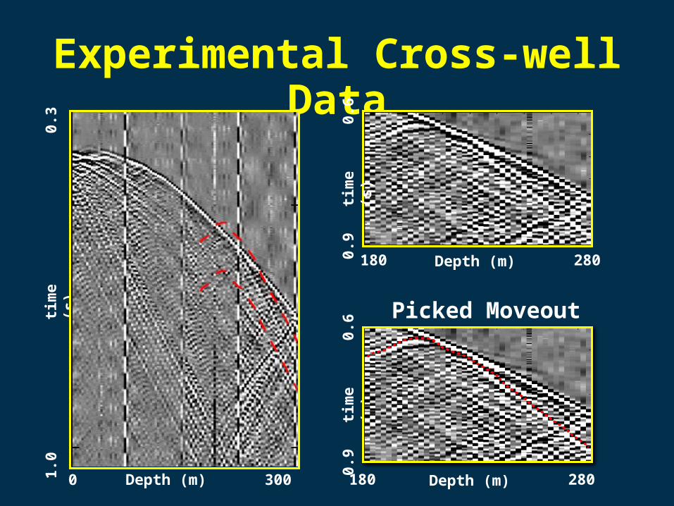
Experimental Cross-well Data

0 Depth (m) 300

0.3

tim

e (s

)1.

0

180 Depth (m) 280

0.6

tim

e (s

)0.

9

Picked Moveout

0.6

tim

e (s

)0.

9

180 Depth (m) 280


180 Depth (m) 280

0.6

tim

e (s

)0.

9

180 Depth (m) 280

0.6

tim

e (s

)0.

9

Median Filter

Time Windowed

180 Depth (m)

0.6

tim

e (s

)0.

9

280

Super-virtual Diffractions


0 Depth (m) 300

0.3

tim

e (s

)1.

0

180 Depth (m) 280

0.6

tim

e (s

)0.

9

Super-virtual Diffraction

0.6

tim

e (s

)0.

9

Median Filtered

180 Depth (m) 280

• Super-virtual diffraction algorithm can greatly improve

the SNR of diffracted waves..

Limitation• Dependence on median filtering when there are other coherent

events.• Wavelet is distorted (solution: deconvolution or match filter).




migration



• Summary

Chapter 2: Multisource LSRTM

• Multisource LSRTM is implemented with random encoding

functions.

LSM produces high quality image. Multisource technique increases computational

efficiency.

Multisource LSRTM, 8 Supergather

Chapter 2: Frequency-selection LSRTM

• Multisource LSRTM is implemented with frequency-

selection encoding functions.

Applicable to marine data.

Frequency-selection LSRTM

• Super-virtual diffraction algorithm can extract diffraction

waves and greatly improve its SNR.

Chapter 4: Super-virtual inteferometric diffractions

Before Before After

Acknowledgements

I thank the sponsors of CSIM consortium for their financial support.

I thank my advisor Prof. Gerard T. Schuster and other committee members for the supervision

over my program of study.

I thank my fellow graduate students for the collaborations and help over last 4 years.

WorkflowRaw data

Pick a master trace

Cross-correlate all the traces with the master trace

Repeat for all the shots and stack the result to give virtual diffractions

Convolve the virtual diffractions with the master trace to restore original traveltime

Stack to generate Super-virtual Diffractions

Diffraction Waveform Modeling

Born

Modeling

0 Distance (km) 3.8

0D

epth

(km

)1.

20

Dep

th (

km)

1.2

0ti

me

(s)

4.0

0 Distance (km) 3.8

Velocity

Reflectivity

Diffraction Waveform Inversion

0 Distance (km) 3.8

0D

epth

(km

)1.

20

Dep

th (

km)

1.2

Initial Velocity

Estimated Reflectivity

0D

epth

(km

)1.

2

Inverted Velocity

0 Distance (km) 3.8

0D

epth

(km

)1.

2

True Velocity

Documents

Multisource Least-squares Reverse Time Migration Wei Dai