Embed Size (px)
Citation preview
HAL Id: tel-01400625https://tel.archives-ouvertes.fr/tel-01400625v2
Submitted on 12 Dec 2016
HAL is a multi-disciplinary open accessarchive for the deposit and dissemination of sci-entific research documents, whether they are pub-lished or not. The documents may come fromteaching and research institutions in France orabroad, or from public or private research centers.
L’archive ouverte pluridisciplinaire HAL, estdestinée au dépôt et à la diffusion de documentsscientifiques de niveau recherche, publiés ou non,émanant des établissements d’enseignement et derecherche français ou étrangers, des laboratoirespublics ou privés.
Multisite Management of Scientific Workflows in theCloudJi Liu
To cite this version:Ji Liu. Multisite Management of Scientific Workflows in the Cloud. Distributed, Parallel, and ClusterComputing [cs.DC]. Université de Montpellier, 2016. English. <tel-01400625v2>
Délivré par l’Université de Montpellier
Préparée au sein de l’école doctorale I2S∗Et de l’unité de recherche UMR 5506
Spécialité: Informatique
Présentée par Ji [email protected]
Gestion multisite de workflowsscientifiques dans le cloud
Soutenue le 03/11/2016 devant le jury composé de :
M. Pascal MOLLI Professeur Université de Nantes Rapporteur
M. Sébastien MONNET Professeur Université de Savoie Rapporteur
Mme. Christine MORIN Directrice de recherche INRIA Examinatrice
Mme. Marta MATTOSO Professeur COPPE / Federal University of Rio de Janeiro Co-encadrante
Mme. Esther PACITTI Professeur Université de Montpellier Co-directrice
M. Patrick VALDURIEZ Directeur de recherche INRIA Co-directeur
∗ I2S: ÉCOLE DOCTORALE INFORMATION STRUCTURES SYSTÈMES


Don’t lose faith,as long as the unremittingly,you will get some fruits.
—Hsue-Chu Tsien

ii
Dedication
To my family.
Acknowledgments
First, I would like to express my sincere appreciation to my advisors: Esther Pacitti,Patrick Valduriez and Marta Mattoso for their patient, helpful, effective guidance. Theygave me excellent advice to improve my writing skills, helped me to develop my ownideas and corrected my papers, posters, articles. In addition, they offered me many op-portunities to connect with reputable experts in different disciplines.
I would like to also thank my family: Jirong Liu and Xiuqin Hao, for giving birth tome and providing me with continuous encouragement and support. You make me strongin heart so that I could pursue my dreams without hesitation.
I am also deeply grateful to my committee members, Pascal Molli and Sébastien Mon-net and my evaluator Christine Morin for spending their time to evaluate my thesis.
I would like to express my gratitude towards my internship supervisors and collabo-rators at Microsoft, Seattle, USA: Vinod Nair, Markus Weimer, Sriram Rao and RaghuRamakrishnan. I am thankful to the collaborators and contributors during my thesis. ToGabriel Antoniu, Alexandru Costan, Luis Pineda-Morales, Radu Tudoran, Raghu Ra-makrishnan, Olivier Nano, Laurent Massoulie and Pierre-Louis Xech for the great collab-oration that we had in the Z-CloudFlow project. To Vítor Silva, Daniel de Oliveira andKary Ocaña for our productive collaboration in the MUSIC project. I would also like tothank Weiwei Chen, who helped me with the experiments and gave me valuable advice onmy ideas. Special thanks go to Idy Camara, Leye Wang, Qiu Han, Yue Li, Haoyi Xiongand Xin Jin, who offered me their advice on my research and my career planning. Thanksalso go to Amelie Chi Zhou, who shared her valuable research experience with me.
I would also like to record my sincere thanks to all the current and former members ofthe Zenith team. Special thanks to Reza Akbarinia, Maximilien Servajean, Miguel Liroz,Mohamed Reda Bouadjenek, Saber Salah, Oleksandra Levchenko and Rim Moussa, whogave me helpful advice on my research work. Thanks also go to Tristan Allard, FlorentMasseglia, Daniel Gaspar, Djamel-Edine Yagoubi, Sen Wang and Carlyna Bondiombouy,with whom, I often recall the happy time we spent together.
I am grateful to my friends who are particular helpful along this path. Thanks go toZhan Li, Wenlong Liu and Liuyang Zhang for all the fun we had and their help on mythesis.
Finally, I would like to thank everyone at UM, LIRMM, MSR-INRIA, INRIA andall the other people who had a direct or indirect contribution to this work and were notmentioned above. I appreciate their help and support.
iii

Résumé
Les workflows scientifiques (SWfs) permettent d’exprimer facilement des activités de cal-cul sur des données, comme charger des fichiers d’entrée, exécuter des analyses, et agré-ger les résultats. Un SWf décrit les dépendances entre les activités, généralement commeun graphe où les nœuds sont des activités et les arêtes représentent les dépendances entreles activités. Les SWfs sont souvent orientés-données, manipulant de grandes quantitésde données. Afin d’éxecuter des SWfs orientés-données dans un temps raisonnable, lessystèmes de gestion de workflows scientifiques (SWfMSs) peuvent être utilisés et déployésdans un environnement de calcul à haute performance (HPC).
Parce qu’il offre des services stables et des ressources de calcul et de stockage quasi-ment infinies à un coût raisonnable, le cloud devient attractif pour l’exécution de SWfs.Un cloud est généralement constitué de plusieurs sites (ou data centers), chacun avecses propres ressources et données. L’exécution de SWf doit alors être adaptée à un cloudmultisite tout en exploitant les ressources de calcul ou de stockage distribuées.
Dans cette thèse, nous étudions le problème d’exécution efficace des SWfs orientés-données dans un cloud multisite. La plupart des SWfMSs ont été conçus pour des clustersou grilles, et quelques uns ont été étendus pour le cloud, en les déployant simplementdans des machines virtuelles (VMs), mais seulement pour un seul site. Pour résoudre leproblème dans le cas multisite, nous proposons une approche distribuée et parallèle quiexploite les ressources disponibles de chaque site. Pour exploiter le parallélisme, nousutilisons une approche algébrique, qui permet d’exprimer les activités en utilisant desopérateurs et les transformer automatiquement en de multiples tâches.
La principale contribution de la thèse est une architecture multisite et des techniquesdistribuées pour exécuter les SWfs. Les principales techniques utilisent des algorithmesde partitionnement de SWf, un algorithme dynamique pour le provisionnement de VMs,un algorithme d’ordonnancement des activités et un algorithme d’ordonnancement detâches. Les algorithmes de partitionnement de SWfs décomposent un SWf en plusieursfragments, chacun pour un site différent. L’algorithme dynamique pour le provisionne-ment de VMs est utilisé pour créer une combinaison optimale de VMs pour exécuter desfragments à chaque site. L’algorithme d’ordonnancement des activités distribue les frag-ments vers les sites, selon un modèle de coût multi-objectif, qui combine à la fois tempsd’exécution et coût monétaire. L’algorithme d’ordonnancement de tâches distribue direc-tement des tâches sur les différents sites en réalisant l’équilibrage de charge au niveau dechaque site. Nos expérimentations montrent que notre approche peut réduire considéra-blement le coût global de l’exécution de SWfs dans un cloud multisite.
v
vi 0. Résumé
Titre en français
Gestion multisite de workflows scientifiques dans le cloud
Mots-clés
• Workflow scientifique
• Système de gestion de workflows scientifiques
• Multisite cloud
• Ordonnancement
Abstract
Scientific Workflows (SWfs) allow scientists to easily express multi-step computationalactivities, such as load input data files, process the data, run analyses, and aggregate theresults. A SWf describes the dependencies between activities, typically as a graph wherethe nodes are activities and the edges express the activity dependencies.
SWfs are often data-intensive, i.e. process, manage or produce huge amounts of data.In order to execute data-intensive SWfs within a reasonable time, Scientific WorkflowManagement Systems (SWfMSs) can be used and deployed in High Performance Comput-ing (HPC) environments (cluster, grid or cloud). By offering stable services and virtuallyinfinite computing, and storage resources at a reasonable cost, the cloud becomes ap-pealing for SWf execution. SWfMSs can be easily deployed in the cloud using VirtualMachines (VMs). A cloud is typically made of several sites (or data centers), each withits own resources and data. Since a SWf may process data located at different sites, SWfexecution should be adapted to a multisite cloud while exploiting distributed computingor storage resources.
In this thesis, we study the problem of efficiently executing data-intensive SWfs in amultisite cloud, where each site has its own cluster, data and programs. Most SWfMSshave been designed for computer clusters or grids, and some have been extended to op-erate in the cloud, but only for single site. To address the problem in the multisite case,we propose a distributed and parallel approach that leverages the resources available atdifferent cloud sites. To exploit parallelism, we use an algebraic approach, which al-lows expressing SWf activities using operators and automatically transforming them intomultiple tasks.
The main contribution is a multisite architecture for SWfMSs and distributed tech-niques to execute SWfs. The main techniques consist of SWf partitioning algorithms, adynamic VM provisioning algorithm, an activity scheduling algorithm and a task schedul-ing algorithm. SWf partitioning algorithms partition a SWf to several fragments, each tobe executed at a different cloud site. The VM provisioning algorithm is used to dynam-ically create an optimal combination of VMs for executing workflow fragments at eachcloud site. The activity scheduling algorithm distributes the SWf fragments to the cloudsites based on a multi-objective cost model, which combines both execution time andmonetary cost. The task scheduling algorithm directly distributes tasks among differentcloud sites while achieving load balancing at each site. Our experiments show that ourapproach can reduce considerably the overall cost of SWf execution in a multisite cloud.
vii
viii 0. Abstract
Title in English
Multisite Management of Scientific Workflows in the Cloud
Keywords
• Scientific workflow
• Scientific workflow management system
• Multisite cloud
• Scheduling

ix
Equipe de RechercheZenith Team, INRIA & LIRMM
LaboratoireLIRMM - Laboratoire d’Informatique, Robotique et Micro-électronique de Montpellier
AdresseUniversité MontpellierBâtiment 5CC 05 018Campus St Priest - 860 rue St Priest34095 Montpellier cedex 5

Résumé Étendu
IntroductionLes workflows scientifiques (SWfs) permettent d’exprimer des activités de calcul à étapesmultiples, p. ex. charger les fichiers d’entrée, traiter les données, exécuter les analyses,et agréger les résultats. Les activités de calcul sont liées par des dépendances. Un SWfdécrit les activités et les dépendances généralement sous forme de graphe, où les nœudsreprésentent les activités de calcul et les arêtes représentent les dépendances entre elles.Les SWfs sont largement utilisés dans plusieurs domaines, tels que l’astronomie [59], labiologie [137], la physique [138], la sismologie [56], la météorologie [190], et cetera.
Les SWfs sont souvent orientés-données, c.-à-d. traitent, gèrent ou produisent d’énormesquantités de données. La gestion et la manipulation des SWfs orientés-données avec desoutils traditionnels de programmation (p. ex. des bibliothèques de code, des langages descript) devient très difficile à mesure que la complexité augmente. Par conséquent, lessystèmes de gestion de workflows scientifiques (SWfMSs) ont été spécialement mis aupoint afin de faciliter le traitement de SWfs, qui incluent de nombreux aspects tels quela modélisation, la programmation, le débogage, et l’exécution de SWfs. Les SWfMSspeuvent générer des données de provenance en cours d’exécution des SWfs. Les donnéesde provenance, qui retracent l’exécution de SWfs et la relation entre les données d’entréeet les données de sortie, sont parfois plus importantes que l’exécution elle-même. Pourexécuter les SWfs orientés-données dans un délai raisonnable, les SWfMSs exploitent lestechniques de parallélisme avec des ressources de calcul à haute performance (HPC) dansun environnement de cluster, grille ou cloud. Quelques SWfMSs existants, p. ex., Pegasus[60, 61], Swift [201], et Chiron [139], sont accessibles au public pour l’exécution et lagestion de SWfs. Cependant, la plupart d’entre eux sont conçus pour les environnementsde cluster ou grille. Dans les environnements de cloud, les SWfMSs utilisent générale-ment les mêmes approches conçues pour le calcul de clusters ou de grilles, qui ne sontpas optimisées pour les environnements de cloud.
En offrant des ressources quasi infinies, des services évolutifs et divers, la qualité deservice stable et des politiques de paiement flexibles, le cloud devient une solution at-tractive pour l’exécution de SWfs. Les SWfMSs peuvent être facilement déployés dans lecloud en exploitant des Machines Virtuelles (VMs). Avec une méthode de pay-as-you-go,les utilisateurs de cloud n’ont pas besoin d’acheter des machines physiques et la mainte-nance des machines est assurée par les fournisseurs de cloud. Ainsi, les environnements
xi
xii 0. Résumé Étendu
de cloud deviennent les infrastructures intéressantes pour l’exécution de SWfs.Un cloud est typiquement multisite (composé de plusieurs sites ou centres de don-
nées), avec chacun ses propres ressources et données et est explicitement accessible auxutilisateurs du cloud. En raison d’une faible latence et des problèmes de propriété, lesdonnées sont généralement stockées dans le site de cloud où sont localisées les sources dedonnées. En conséquence, les données d’entrée d’un SWf peuvent être distribuées géo-graphiquement. Par exemple, les données climatiques dans le système terrestre de grille[189], les grandes quantités de données brutes de la chromodynamique quantique (QCD)[149] et les données du projet ALICE [1] sont distribuées géographiquement. Puisqu’unSWf peut traiter des données distribuées géographiquement, l’exécution de SWf doit êtreadaptée à un cloud multisite en exploitant les ressources de calcul ou de stockage dis-tribuées au-delà d’un site de cloud. Les approches existantes restent limitées à des envi-ronments avec un seul cluster, dans une grille ou un cloud, et ne sont pas adaptées à unenvironnement multisite.
Cette thèse a été préparée dans le cadre de deux projets scientifiques : Z-CloudFlow(projet du centre MSR-Inria avec l’équipe Inria Kerdata) et MUSIC (projet FAPERJ-Inriaavec des équipes de Rio de Janeiro) avec l’objectif principal d’exécuter efficacement lesSWfs orientés-données dans un cloud multisite, où chaque site a son propre cluster, sesdonnées et ses programmes. Cette thèse contient 5 chapitres principaux : état de l’art,partitionnement de SWfs, provisionnement de VMs dans un seul site, ordonnancementmulti-objectif de SWfs dans un cloud multisite et ordonnancement de tâches avec lesdonnées de provenance. Elle commence par un chapitre d’introduction et se termine parun chapitre de conclusion qui résume les contributions et propose des directions de re-cherche futures.
État de l’artUn SWf est l’assemblage d’activités scientifiques de traitement de données avec des dé-pendances de données entre elles [57]. Un SWfMS est un outil efficace pour exécuter lesSWfs et gérer des ensembles de données dans différents environnements informatiques.Afin d’exécuter un SWf dans un environnement donné, un SWfMS génère un plan d’exé-cution de workflow (WEP), qui est un programme qui saisit les décisions d’optimisation etles directives d’exécution, typiquement le résultat de la compilation et l’optimisation d’unworkflow, avant l’exécution. Cette section présente les techniques existantes de SWfs etSWfMSs, y compris l’architecture fonctionnelle, les techniques de parallélisation, l’ana-lyse de SWfMSs différents et l’environnement de cloud multisite.
L’architecture fonctionnelle d’un SWfMS peut être décrite en couches comme suit[60, 201, 21, 139] : présentation, services aux utilisateurs, génération de WEP, exécutionde WEP et infrastructures. Un utilisateur interagit avec un SWfMS à travers la couche deprésentation et réalise les fonctions souhaitées dans la couche de services aux utilisateurs.La couche de services d’utilisateur prend généralement en compte les données de prove-nance, qui sont les métadonnées qui capturent l’histoire de dérivation d’un ensemble de
xiii
données. Un SWf est traité dans la couche de génération de WEP pour produire un WEP,qui est exécuté dans la couche d’exécution de WEP. Afin de réduire le temps d’exécu-tion, les SWfs sont généralement exécutés en parallèle. Le SWfMS accède aux ressourcesphysiques à travers la couche d’infrastructure pour l’exécution de SWfs.
L’exécution en parallèle de SWfs comprend le parallélisme et l’ordonnancement. Leparallélisme de SWfs identifie les tâches qui peuvent être exécutées en parallèle. Il y adeux niveaux de parallélisme : le parallélisme à gros grain et le parallélisme à grain fin.Le parallélisme à gros grain, qui est effectué au niveau de SWf, est obtenu en exécutantdes fragments de SWfs en parallèle. Un fragment de SWf (ou fragment pour faire court)peut être défini comme un sous-ensemble des activités et des dépendances de donnéesd’un SWf original, qui est généré par le partitionnement de SWf. Le parallélisme à grainfin réalise le parallélisme en exécutant différentes activités en parallèle dans un SWf ouun fragment du SWf. L’ordonnancement de SWfs est un processus d’attribution de tâchesaux ressources informatiques (c.-à-d. nœuds de calcul) à exécuter [33]. Les méthodesd’ordonnancement peuvent être statiques, dynamiques ou hybrides. L’ordonnancementstatique génère un plan d’ordonnacement (SP) qui attribue toutes les tâches exécutablesaux nœuds de calcul avant l’exécution et le SWfMS respecte strictement le SP pendanttoute l’exécution de SWf [33]. Il est efficace lorsque l’environnement d’exécution variepeu au cours de l’exécution de SWfs, et quand le SWfMS a suffisamment d’informa-tions sur les capacités informatiques et de stockage des nœuds de calcul correspondants.L’ordonnancement dynamique produit des SPs qui distribuent les tâches exécutables auxnœuds de calcul lors de l’exécution de SWfs [33]. Ce type d’ordonnacement est appro-prié pour les SWfs dont la charge de travail des tâches est difficile à estimer, ou pour lesenvironnements où les capacités des nœuds de calcul varient beaucoup pendant l’exécu-tion. Les méthodes d’ordonnancement statiques et dynamiques ont leurs propres avan-tages. Elles peuvent être combinées en méthode d’ordonnacement hybride pour obtenirde meilleures performances.
Nous avons étudié huit SWfMSs typiques : Pegasus, Swift, Kepler, Taverna, Chiron,Galaxy, Triana [173], Ascalon [68] ; ainsi que le portail de SWfMSs WS-PGRADE/gUSE[105]. Pegasus et Swift ont un excellent soutien sur l’évolutivité et la haute performancede SWfs orientés-données. Pegasus, Swift, Kepler, Taverna et WS-PGRADE/gUSE sontlargement utilisés dans l’astronomie, la biologie, et cetera. Par contre, Galaxy ne peutexécuter que les SWfs bioinformatiques. Tous les frameworks supportent le parallélismeà grain fin, l’ordonnancement dynamique et trois d’entre eux (Pegasus, Kepler et WS-PGRADE/gUSE) supportent l’ordonnancement statique. Tous ces systèmes supportentl’exécution de SWfs dans l’environnement de grille et de cloud. Chiron exploite une ap-proche algébrique [146] pour gérer l’exécution en parallèle de SWfs orientés-données. Ilutilise un modèle de données algébriques pour exprimer toutes les données comme lesrelations et représentent les activités de SWfs comme des expressions algébriques dans lacouche de présentation. Une relation contient des ensembles de tuples composés d’attri-buts de base. Une expression algébrique consiste en activités algébriques, opérandes sup-plémentaires, opérateurs et relations d’entrée et de sortie. Une activité algébrique contientun programme ou une expression SQL, et les schémas de relations d’entrée et de sortie.
xiv 0. Résumé Étendu
Un opérande supplémentaire est l’information latérale pour l’expression algébrique, quipeut être une relation ou un ensemble d’attributs de regroupement. Il y a six opérateursqui peuvent automatiquement transformer une activité en de multiples tâches à exécuter.
Il y a des cas importants où les SWfs devront être exécutés sur plusieurs sites decloud, p. ex. parce que les données accessibles par le SWf sont dans les bases de donnéesde différents groupes de recherche dans les différents sites ou parce que l’exécution d’unSWf a besoin de plus de ressources que celles d’un seul site. Les grands fournisseurs decloud tels que Microsoft et Amazon ont généralement plusieurs centres de données distri-bués géographiquement dans les différents sites. Dans un cloud multisite, nous pouvonsexécuter un SWf avec le parallélisme à grain fin ou le parallélisme à gros grain au ni-veau multisite. L’exécution de SWfs avec le parallélisme à grain fin est d’attribuer toutesles tâches dans chaque site de cloud. Bien qu’il existe des méthodes d’ordonnancement[65, 145], elles n’ont pas de support à la gestion des données de provenance, celles quisont importantes pour l’exécution de SWfs. Avec le parallélisme à gros grain, un SWf estpartitionné en fragments. Chaque fragment est affecté à un site spécifique et ses tâchessont allouées dans les VMs de ce site. Certaines méthodes [38, 39] sont proposées pourpermettre d’exécuter les SWfs dans un cloud multisite par le partitionnement de SWfs, ilsse concentrent généralement sur un seul objectif, c.-à-d. la réduction du temps d’exécu-tion, avec une contrainte de stockage mais le cas multi-objectif reste un problème, p. ex.réduire à la fois le temps d’exécution et le coût monétaire. En outre, ils n’ont générale-ment pas de support pour le provisionnement dynamique de VMs dans le cloud, ce qui estessentiel pour l’exécution dans un environnement de cloud. Chiron est adapté au cloudgrâce à son extension, Scicumulus [51, 52], qui supporte le provisionnement de calculdynamique [50]. Cependant, cette approche se concentre sur un environnement de cloudmono site.
Partitionnement de SWfsNous attaquons le problème de partitionnement de SWfs afin d’exécuter les SWfs dansun cloud multisite. Notre objectif principal est de permettre l’exécution de SWfs dans uncloud multisite pour partitionner les SWfs en fragments afin de réduire le temps d’exé-cution, tout en assurant que certaines activités soient exécutées sur les sites de cloudspécifiques.
Il y a essentiellement deux techniques de partitionnement de SWfs, c.-à-d. le partition-nement de DAG et le partitionnement de données. Le partitionnement de DAG transformeun DAG composé des activités en un DAG composé des fragments tandis que chaquefragment est un DAG composé des activités et des dépendances. Le partitionnement dedonnées divise les données d’entrée d’un fragment généré par le partitionnement de DAGen plusieurs ensembles de données, dont chacun est encapsulé dans un fragment nouvel-lement généré. Nous nous concentrons sur le partitionnement de DAG dans ce travail. Ily a une technique de partitionnement général, c.-à-d. l’encapsulation des activités, quiencapsule chaque activité dans un fragment de SWf.
xv
Nous proposons trois méthodes de partitionnement de SWfs, c.-à-d. la confidentialitéscientifique (SPr), la minimisation de la transmission de données (DTM) et l’adaptationde la capacité informatique (CCA). SPr partitionne les SWfs en mettant les activités deblocage et ses activités suivantes disponibles à un fragment, pour mieux supporter la sur-veillance de l’exécution sous la contrainte de sécurité. DTM partitionne les SWfs avec laprise en compte des activités de blocage, tout en minimisant le volume de données à trans-férer entre les fragments de SWfs différents. CCA partitionne les SWfs selon la capacitéde calcul de différents sites de cloud. Cette technique tente de mettre plus d’activités aufragment à exécuter dans un site de cloud avec une plus grande capacité de calcul. Nostechniques de partitionnement sont adaptées aux différentes configurations de cloud afinde réduire le temps d’exécution des SWfs. De plus, nous proposons également d’utiliserdes techniques de raffinage de données, c.-à-d. la combinaison de fichiers et la compres-sion de données, afin de réduire le temps de la transmission de données entre les différentssites.
Nous prenons Buzz SWf [64] comme un cas d’utilisation et adaptons Chiron pourl’exécution de SWfs dans le cloud multisite. Nous évaluons largement nos techniquesde partitionnement proposées en exécutant Buzz avec Chiron déployé dans deux sites,c.-à-d. Europe occidentale et l’Est des États-Unis, du cloud Azure. Nous considéronsdeux configurations de cloud : homogène et hétérogène. Le cas où tous les sites ont lesmêmes nombres et types de VMs correspond à la configuration homogène tandis que dansune configuration hétérogène les sites ont des nombres ou types de VMs différents. Lesrésultats de nos expérimentations montrent que DTM avec des techniques de raffinagede données est adapté (24, 1% du temps épargné par rapport à ACC sans raffinage dedonnées) à exécuter les SWfs dans un cloud multisite avec une configuration homogène,et qu’ACC fonctionne mieux (28, 4% du temps épargné par rapport à la technique SPr sansraffinage de données) avec une configuration hétérogène. En outre, les résultats montrentque les techniques de raffinage de données peuvent réduire considérablement le temps dela transmission de données entre deux sites différents.
Provisionnement de VMs dans un siteNous traitons le problème de la génération de plans de provisionnement de VMs pourl’exécution de SWfs dans un seul site de cloud pour plusieurs objectifs. Notre princi-pale contribution est de proposer un modèle de coût et un algorithme afin de générer desplans de provisionnement de VMs pour réduire à la fois le temps d’exécution et le coûtmonétaire pour l’exécution de SWfs dans un seul site de cloud.
Pour résoudre le problème, nous concevons un modèle de coût multi-objectif pourl’exécution de SWfs dans un seul site de cloud. Le modèle de coût est une fonction pon-dérée avec les objectifs de réduction du temps d’exécution et le coût monétaire basé sur letemps d’exécution et le coût monétaire souhaité par les utilisateurs. L’importance de l’ob-jectif du temps d’exécution doit être supérieure à zéro et inférieure à 1, p. ex. 0.1 ou 0.9.Notre modèle de coût considère la charge de travail séquentiel et le coût pour démarrer
xvi 0. Résumé Étendu
les VMs, qui est plus précis par rapport aux modèles de coûts existants, p. ex. GraspCC[47]. Le temps d’exécution estimé est basé sur la loi d’Amdahl [170]. Le coût monétaireestimé est basé sur le temps d’exécution estimé et le coût monétaire pour utiliser des VMsdans une unité de temps.
En nous appuyant sur le modèle de coût, nous proposons un algorithme de provision-nement dans un seul site (SSVP) pour générer des plans de provisionnement à exécuter lesSWfs dans un seul site de cloud. SSVP calcule d’abord un nombre optimal de cœurs deprocesseurs pour l’exécution de SWfs basé sur le modèle de coût multi-objectif. Ensuite,il génère un plan de provisionnement et améliore itérativement le plan de provisionne-ment afin de réduire le coût basé sur le modèle de coût et le nombre optimal de cœurs deprocesseurs. Enfin, SSVP génère un plan de provisionnement de VMs correspondant aucoût minimum pour exécuter les SWfs avec l’importance spécifique de chaque objectif.
Nous avons réalisé des évaluations approfondies à comparer notre modèle de coût etcelui de GraspCC. Nous avons exécuté le workflow SciEvol [137] avec différentes quan-tités de données d’entrée et de différentes importance du temps d’exécution, en déployantChiron dans le site de l’Est du Japon du cloud d’Azure. Les résultats des expérimentationsmontrent que notre algorithme peut adapter les plans de provisionnement de VMs aux dif-férentes configurations, c.-à-d. générer différents plans de provisionnement de VMs pourles différentes importances du temps d’exécution. SSVP génère de meilleurs plans deprovisionnement (53, 6%) par rapport à GraspCC. Les résultats révèlent également quenotre modèle de coût est plus (76, 7%) précis pour estimer le temps d’exécution et le coûtmonétaire par rapport à GraspCC, en raison de la prise en compte de la charge de travailséquentiel et le coût pour démarrer les VMs.
Ordonnancement multi-objectif de SWfs dans un cloud mul-tisiteNous résolvons le problème de l’ordonnancement des fragments de SWfs avec plusieursobjectifs, afin de permettre l’exécution de SWfs dans un cloud multisite avec une contraintede données stockées. Nous imaginons que les données stockées dans un site spécifique nepeuvent pas être autorisées à être transférées vers d’autres sites en raison de la propriétéou grandes quantités de données, qui s’appelle la contrainte de données stockées. Dansce travail, nous avons pris en compte les différents prix des VMs et les données stockéesdans des sites différents.
Le modèle de coût multisite est une fonction pondérée composée du temps d’exécutionet du coût monétaire basé sur le temps d’exécution et le coût monétaire souhaité parl’utilisateur. Toutefois, puisqu’il est difficile d’estimer le temps d’exécution et le coûtmonétaire globale pour exécuter un SWf dans un cloud multisite, nous proposons unmodèle de coût multisite comme une combinaison du coût pour exécuter chaque fragmentdu SWf. Nous décomposons également le temps d’exécution et le coût monétaire souhaitéd’un SWf en une combinasion de ceux de chaque fragment du SWf. Basé sur le tempsd’exécution et le coût monétaire souhaité de chaque fragment du SWf, on peut estimer
xvii
le coût pour exécuter chaque fragment du SWf sur un site prévu basé sur le modèle decoût correspondant à SSVP. Enfin, notre modèle de coût multisite peut estimer le coûtglobal en considérant le coût à transférer des données à travers différents sites avec unplan d’ordonnancement.
Nous présentons deux algorithmes d’ordonnancement que nous avons adaptés, l’or-donnancement basé sur les localisations de données (LocBased) et l’ordonnancementgourmand de sites (SGreedy), et l’algorithme que nous proposons : l’ordonnancementgourmand des activités (ActGreedy). LocBased exploite DTM à partitionner les SWfset attribue les fragments aux sites où les données d’entrée sont stockées. Cet algorithmeignore le coût monétaire et peut encourir un coût énorme à exécuter les SWfs. SGreedyprend l’avantage de la technique d’encapsulation des activités pour partitionner les SWfset attribue le meilleur fragment à chaque site. Il attribue les activités d’un pipeline desactivités aux sites différents, qui conduit à une grande transmission de données intersiteet un temps d’exécution plus long. ActGreedy partitionne les SWfs avec la techniqued’encapsulation des activités et regroupe de petits fragments en plus gros fragments pourréduire la transmission de données entre les différents sites et attribue chaque fragment aumeilleur site. Cet algorithme permet de réduire le temps d’exécution global en comparantle coût pour exécuter des fragments dans chaque site, qui est généré basé sur SSVP.
Nous avons évalué notre algorithme d’ordonnancement en exécutant SciEvol avecdifférentes quantités de données d’entrée et les différentes importances des objectifs danstrois sites du cloud d’Azure. Les trois sites de cloud sont l’Ouest de l’Europe, l’Ouest duJapon, et l’Orient du Japon et les coûts d’utilisation de VMs sur chaque site sont différents.Nous avons utilisé SSVP pour générer des plans de provisionnement de VMs et Chironpour exécuter des fragments du SWf dans chaque site. Les résultats des expérimentationsmontrent qu’ActGreedy fonctionne mieux en termes du coût pondéré pour exécuter lesSWfs dans un cloud multisite par rapport à LocBased (jusqu’à 10.7%) et SGreedy (jus-qu’à 17, 2%). En outre, les résultats révèlent également que le temps d’ordonnancementd’ActGreedy est raisonnable par rapport aux deux approches générales, c.-à-d. Brut Forceet Genetic.
Ordonnancement de tâches avec les données de provenanceNous traitons le problème d’ordonnancement de tâches pour l’exécution de SWfs en mul-tisite avec le soutien sur les données de provenance. L’objectif principal est de permettrel’exécution de SWfs avec les données d’entrée distribuées dans les différents sites dansun délai minimum avec le soutien sur les données de provenance, tandis que les bandespassantes entre les différents sites sont différentes. Dans ce travail, nous proposons ChironMultisite et un algorithme d’ordonnancement de tâches.
Chiron Multisite est une extension de Chiron pour les environnements de cloud mul-tisite. Chiron met en œuvre une approche algébrique pour exprimer les SWfs et optimiserl’exécution de SWfs dans un seul site. Chiron Multisite permet d’exécuter simultané-ment des tâches d’une activité sur des sites différents pour traiter les données distribuées.

xviii 0. Résumé Étendu
Nous proposons aussi le modèle de provenance multisite pour Chiron Multisite. Dans uncloud multisite, nous proposons différentes méthodes pour le transfert de données inter-site. Nous utilisons notre méthode d’ordonnancement à deux niveaux, c.-à-d. l’ordonnan-cement multisite et l’ordonnancement d’un seul site, pour l’ordonnancement de tâchesdans un cloud multisite. Multisite Chiron correspond au parallélisme à grain fin au ni-veau multisite, qui permet aux différentes tâches d’un fragment d’être exécutées dans lesdifférents sites de cloud.
Nous proposons un algorithme de l’ordonnancement multisite de tâches orientés-données (DIM) pour attribuer des tâches au niveau multisite en considérant le support desdonnées de provenance, différentes bandes passantes entre les différents sites et la distri-bution de données d’entrée. D’abord, DIM attribue les tâches en fonction de localisationsde données sur différents sites. Puis, il redistribue les tâches afin d’atteindre l’équilibrede charge entre les différents sites de cloud basés sur un modèle de coût pour estimer lacharge d’exécution de chaque site. L’équilibre de charge représente qu’il faut exécuterles tâches dans le même temps dans chaque site. Le modèle de coût prend en compte letemps de transférer les données d’entrée des tâches entre les différents sites et le temps detransférer les données de provenance à une base de données centralisée.
Nous avons évalué nos algorithmes avec Chiron Multisite en exécutant Buzz et Mon-tage [6] dans trois sites de cloud Azure, c.-à-d. US centrale, l’Ouest de l’Europe et le Nordde l’Europe. Nous avons exécuté buzz avec différentes quantités de données d’entrée etMontage avec différents degrés en utilisant le Chiron Multisite. Les résultats expérimen-taux montrent que DIM est beaucoup mieux que deux algorithmes d’ordonnancementexistants, c.-à-d. MCT (jusqu’à 24, 3%) et OLB (jusqu’à 49, 6%), en termes du tempsd’exécution. DIM peut également réduire de manière significative (jusqu’à plus de 7 fois)les données transférées entre les sites, comparé avec MCT et OLB. En outre, les résultatsrévèlent également que le temps d’ordonnancement de DIM est raisonnable par rapportà la durée d’exécution globale de SWfs (moins de 3%). En particulier, les expérimenta-tions montrent que la distribution de tâches est adaptée en fonction de différentes bandespassantes entre les différents sites pour la génération de données de provenance.
ConclusionDans cette thèse, nous avons traité le problème de l’exécution de SWfs orientés-donnéesdans un cloud multisite, où les données et les ressources informatiques peuvent être dis-tribués aux différents sites de cloud. Pour cette raison, nous avons proposé une approchedistribuée et parallèle qui exploite les ressources disponibles dans les différents sites decloud. Dans notre étude de l’état de l’art, nous avons proposé une architecture fonction-nelle de SWfMS en analysant et en catégorisant les techniques existantes. Pour exploiterle parallélisme, nous avons utilisé une approche algébrique, ce qui permet d’exprimerles activités de SWfs en utilisant des opérateurs à automatiquement les transformer ende multiples tâches. Nous avons proposé l’algorithmes de partitionnement de SWfs, unalgorithme dynamique de provisionnement de SWfs dans un seul site, un algorithme d’or-
xix
donnancement multi-objectif dans un cloud multisite, un algorithme d’ordonnancementde tâches avec les données de provenance et Chiron Multisite. Différents algorithmesde partitionnement de SWfs partitionnent un SWf à plusieurs fragments. L’algorithme deprovisionnement de VMs est utilisé pour créer dynamiquement une combinaison optimalede VMs pour exécuter des fragments d’un SWf dans chaque site de cloud. L’algorithmed’ordonnancement multi-objectif distribue les fragments d’un SWf aux sites de cloud avecle coût minimum basé sur un modèle de coût multi-objectif. L’algorithme d’ordonnance-ment de tâches distribue directement des tâches entre les différents sites de cloud tout enréalisant l’équilibrage de charge au niveau de chaque site basé sur un SWfMS multisite,Chiron Multisite. Chiron Multisite est une extension de Chiron pour exécuter les SWfsdans les environnements de cloud multisite. Nous avons évalué nos solutions proposées enexécutant des SWfs réels dans le cloud de Microsoft Azure. Nos résultats expérimentauxmontrent les avantages de nos solutions par rapport aux techniques existantes.
Nos contributions peuvent être utilisées comme le point de départ pour la recherchefuture. Nous proposons les futures directions de recherche suivantes :
• Distribution de la provenance. La gestion de données de provenance distribuéespeut réduire le temps de générer ou de récupérer des données de provenance danschaque site afin de réduire le temps d’exécution global de SWfs dans un cloudmultisite.
• Transfert de données. Une solution possible de transférer efficacement des don-nées entre deux sites de cloud est de sélectionner plusieurs nœuds sur chaque sitepour envoyer ou recevoir des données, en exploitant le transfert de données en pa-rallèle et en faisant le transfert de données plus efficace.
• Spark multisite. Nos algorithmes et optimisations d’ordonnancement multisite pour-raient être adaptées pour le framework Spark pour l’exécution de SWfs dans uncloud multisite.
• Architecture : Une architecture peer-to-peer peut être utilisée pour atteindre la to-lérance aux pannes lors de l’exécution de SWfs dans un seul site de cloud ou uncloud multisite.
• Ordonnancement dynamique. L’ordonnancement dynamique des activités ou destâches peut être mieux adapté à l’environnement d’exécution en considérant lesparamètres mesurés lors de l’exécution de SWfs, p. ex. le coût monétaire des VMs,la bande passante pour transferer ou recevoir des données dans les VMs, etc.
PublicationsLes contributions ont conduit aux publications suivantes :
• Ji Liu, Esther Pacitti, Patrick Valduriez, Daniel de Oliveira and Marta Mattoso.Multi-Objective Scheduling of Scientific Workflows in Multisite Clouds. Dans BDA’
xx 0. Résumé Étendu
2016 : Gestion de données - principles, technologies et applications, 2016. À pa-raître.
• Luis Pineda-Morales, Ji Liu, Alexandru Costan, Esther Pacitti, Gabriel Antoniu,Patrick Valduriez, and Marta Mattoso. Managing Hot Metadata for Scientific Work-flows on Multisite Clouds. Dans IEEE International Conference on Big Data, 2016.À paraître.
• Ji Liu, Esther Pacitti, Patrick Valduriez, Marta Mattoso. Scientific Workflow Sche-duling with Provenance Support in Multisite Cloud. Dans 12th International Mee-ting on High Performance Computing for Computational Science (VECPAR), 2016,1− 8.
• Ji Liu, Esther Pacitti, Patrick Valduriez, Daniel Oliveira, Marta Mattoso. Multi-objective scheduling of Scientific Workflows in multisite clouds. Dans Future Ge-neration Computer Systems, 2016, volume 63, 76− 95.
• Ji Liu, Esther Pacitti, Patrick Valduriez, Marta Mattoso. A Survey of Data-IntensiveScientific Workflow Management. Dans Journal of Grid Computing, 2015, volume13, numéro 4, 457− 493.
• Ji Liu, Esther Pacitti, Patrick Valduriez, Marta Mattoso, Parallelization of ScientificWorkflows in the Cloud, Rapport de recherche RR-8565, 2014.
• Ji Liu, Vítor Silva, Esther Pacitti, Patrick Valduriez, Marta Mattoso. Scientific Work-flow Partitioning in Multi-site Clouds. Dans BigDataCloud’2014 : 3rd Workshopon Big Data Management in Clouds in conjunction with Euro-Par, 2014. Springer,Lecture Notes in Computer Science, 8805, 105− 116.
• Ji Liu. Multisite Management of Data-intensive Scientific Workflows in the Cloud.Dans BDA’2014 : Gestion de données - principles, technologies et applications,2014, 28− 30.
Contents
Acknowledgments iii
Résumé v
Abstract vii
Résumé Étendu xi
1 Introduction 11.1 Thesis Context . . . . . . . . . . . . . . . . . . . . . . . . . . . . . . . 21.2 Contributions . . . . . . . . . . . . . . . . . . . . . . . . . . . . . . . . 31.3 Organization of the Thesis . . . . . . . . . . . . . . . . . . . . . . . . . 6
2 State of the Art 92.1 Overview and Motivations . . . . . . . . . . . . . . . . . . . . . . . . . 92.2 Scientific Workflow Management . . . . . . . . . . . . . . . . . . . . . 11
2.2.1 Basic Concepts . . . . . . . . . . . . . . . . . . . . . . . . . . . 112.2.1.1 Scientific Workflows . . . . . . . . . . . . . . . . . . . 112.2.1.2 Scientific Workflow Life Cycle . . . . . . . . . . . . . 122.2.1.3 Scientific Workflow Management Systems . . . . . . . 132.2.1.4 Scientific Workflow Examples . . . . . . . . . . . . . 13
2.2.2 Functional Architecture of SWfMSs . . . . . . . . . . . . . . . . 162.2.2.1 Presentation Layer . . . . . . . . . . . . . . . . . . . . 162.2.2.2 User Services Layer . . . . . . . . . . . . . . . . . . . 182.2.2.3 WEP Generation Layer . . . . . . . . . . . . . . . . . 202.2.2.4 WEP Execution Layer . . . . . . . . . . . . . . . . . . 222.2.2.5 Infrastructure Layer . . . . . . . . . . . . . . . . . . . 23
2.2.3 Techniques for Data-intensive Scientific Workflows . . . . . . . . 242.3 Parallel Execution in SWfMSs . . . . . . . . . . . . . . . . . . . . . . . 27
2.3.1 Scientific Workflow Parallelism . . . . . . . . . . . . . . . . . . 282.3.1.1 Coarse-Grained Parallelism . . . . . . . . . . . . . . . 282.3.1.2 Fine-Grained Parallelism . . . . . . . . . . . . . . . . 28
2.3.2 Scientific Workflow Scheduling . . . . . . . . . . . . . . . . . . 312.3.2.1 Task Clustering . . . . . . . . . . . . . . . . . . . . . 32
xxi
xxii CONTENTS
2.3.2.2 Static Scheduling . . . . . . . . . . . . . . . . . . . . 322.3.2.3 Dynamic Scheduling . . . . . . . . . . . . . . . . . . 332.3.2.4 Hybrid Scheduling . . . . . . . . . . . . . . . . . . . . 342.3.2.5 Scheduling Optimization Algorithms . . . . . . . . . . 342.3.2.6 Conclusion . . . . . . . . . . . . . . . . . . . . . . . . 35
2.4 SWfMS in a Multisite Cloud . . . . . . . . . . . . . . . . . . . . . . . . 352.4.1 Cloud Computing . . . . . . . . . . . . . . . . . . . . . . . . . . 362.4.2 Multisite Management in the Cloud . . . . . . . . . . . . . . . . 372.4.3 Data Storage in the Cloud . . . . . . . . . . . . . . . . . . . . . 38
2.4.3.1 File Systems . . . . . . . . . . . . . . . . . . . . . . . 392.4.4 Scientific Workflow Execution in the Cloud . . . . . . . . . . . . 41
2.4.4.1 Execution at a Single Cloud Site . . . . . . . . . . . . 422.4.4.2 Execution in a Multisite Cloud . . . . . . . . . . . . . 43
2.4.5 Conclusion and Remarks . . . . . . . . . . . . . . . . . . . . . . 442.5 Overview of Existing Solutions . . . . . . . . . . . . . . . . . . . . . . . 44
2.5.1 Parallel Processing Frameworks . . . . . . . . . . . . . . . . . . 442.5.2 SWfMS . . . . . . . . . . . . . . . . . . . . . . . . . . . . . . . 47
2.5.2.1 Pegasus . . . . . . . . . . . . . . . . . . . . . . . . . 482.5.2.2 Swift . . . . . . . . . . . . . . . . . . . . . . . . . . . 512.5.2.3 Kepler . . . . . . . . . . . . . . . . . . . . . . . . . . 512.5.2.4 Taverna . . . . . . . . . . . . . . . . . . . . . . . . . 532.5.2.5 Chiron . . . . . . . . . . . . . . . . . . . . . . . . . . 542.5.2.6 Galaxy . . . . . . . . . . . . . . . . . . . . . . . . . . 552.5.2.7 Triana . . . . . . . . . . . . . . . . . . . . . . . . . . 552.5.2.8 Askalon . . . . . . . . . . . . . . . . . . . . . . . . . 562.5.2.9 WS-PGRADE/gUSE . . . . . . . . . . . . . . . . . . 56
2.5.3 Concluding Remarks . . . . . . . . . . . . . . . . . . . . . . . . 582.6 Conclusion . . . . . . . . . . . . . . . . . . . . . . . . . . . . . . . . . 58
3 Scientific Workflow Partitioning in a Multisite Cloud 613.1 Overview of the Proposal and Motivations . . . . . . . . . . . . . . . . . 613.2 Related Work . . . . . . . . . . . . . . . . . . . . . . . . . . . . . . . . 633.3 System Model . . . . . . . . . . . . . . . . . . . . . . . . . . . . . . . . 633.4 Use Case: Buzz Workflow . . . . . . . . . . . . . . . . . . . . . . . . . 643.5 Workflow Partitioning Techniques . . . . . . . . . . . . . . . . . . . . . 673.6 Validation . . . . . . . . . . . . . . . . . . . . . . . . . . . . . . . . . . 693.7 Conclusion . . . . . . . . . . . . . . . . . . . . . . . . . . . . . . . . . 71
4 VM Provisioning of Scientific Workflows in a Single Site Cloud 734.1 Motivations and Overview . . . . . . . . . . . . . . . . . . . . . . . . . 734.2 Multi-objective Cost Model . . . . . . . . . . . . . . . . . . . . . . . . . 75
4.2.1 Time Cost . . . . . . . . . . . . . . . . . . . . . . . . . . . . . . 754.2.2 Monetary Cost . . . . . . . . . . . . . . . . . . . . . . . . . . . 77
CONTENTS xxiii
4.3 Single Site VM Provisioning . . . . . . . . . . . . . . . . . . . . . . . . 784.4 Use Case . . . . . . . . . . . . . . . . . . . . . . . . . . . . . . . . . . 814.5 Experimental Evaluation . . . . . . . . . . . . . . . . . . . . . . . . . . 814.6 Conclusion . . . . . . . . . . . . . . . . . . . . . . . . . . . . . . . . . 88
5 Multi-Objective Scheduling of Scientific Workflows in a Multisite Cloud 895.1 Overview and Motivations . . . . . . . . . . . . . . . . . . . . . . . . . 895.2 Related Work . . . . . . . . . . . . . . . . . . . . . . . . . . . . . . . . 915.3 Problem Definition . . . . . . . . . . . . . . . . . . . . . . . . . . . . . 935.4 Multisite SWfMS Architecture . . . . . . . . . . . . . . . . . . . . . . . 955.5 Multi-objective Optimization . . . . . . . . . . . . . . . . . . . . . . . . 96
5.5.1 Multi-objective Cost Model . . . . . . . . . . . . . . . . . . . . 965.5.1.1 Time Cost . . . . . . . . . . . . . . . . . . . . . . . . 975.5.1.2 Monetary Cost . . . . . . . . . . . . . . . . . . . . . . 99
5.5.2 Cost Estimation . . . . . . . . . . . . . . . . . . . . . . . . . . . 1015.6 Fragment Scheduling . . . . . . . . . . . . . . . . . . . . . . . . . . . . 101
5.6.1 Use Case . . . . . . . . . . . . . . . . . . . . . . . . . . . . . . 1015.6.2 Scheduling approaches . . . . . . . . . . . . . . . . . . . . . . . 102
5.6.2.1 Data Location Based Scheduling . . . . . . . . . . . . 1045.6.2.2 Site Greedy Scheduling . . . . . . . . . . . . . . . . . 1045.6.2.3 Activity Greedy Scheduling . . . . . . . . . . . . . . . 1055.6.2.4 Solution analysis . . . . . . . . . . . . . . . . . . . . . 108
5.7 Experimental Evaluation . . . . . . . . . . . . . . . . . . . . . . . . . . 1105.8 Conclusion . . . . . . . . . . . . . . . . . . . . . . . . . . . . . . . . . 122
6 Task Scheduling with Provenance Support in Multisite Clouds 1236.1 Proposal Overview and Motivations . . . . . . . . . . . . . . . . . . . . 1236.2 Related Work . . . . . . . . . . . . . . . . . . . . . . . . . . . . . . . . 1256.3 Problem Definition . . . . . . . . . . . . . . . . . . . . . . . . . . . . . 1266.4 System Design . . . . . . . . . . . . . . . . . . . . . . . . . . . . . . . 128
6.4.1 Single Site Chiron . . . . . . . . . . . . . . . . . . . . . . . . . 1286.4.2 Multisite Chiron . . . . . . . . . . . . . . . . . . . . . . . . . . 130
6.5 Task Scheduling . . . . . . . . . . . . . . . . . . . . . . . . . . . . . . . 1326.5.1 Single Site Task Scheduling . . . . . . . . . . . . . . . . . . . . 1326.5.2 Multisite Task Scheduling . . . . . . . . . . . . . . . . . . . . . 1326.5.3 Complexity . . . . . . . . . . . . . . . . . . . . . . . . . . . . . 1356.5.4 Execution Time Estimation . . . . . . . . . . . . . . . . . . . . . 136
6.6 Experimental Evaluation . . . . . . . . . . . . . . . . . . . . . . . . . . 1376.6.1 SWf Use Cases . . . . . . . . . . . . . . . . . . . . . . . . . . . 137
6.6.1.1 Buzz Workflow . . . . . . . . . . . . . . . . . . . . . 1386.6.1.2 Montage Workflow . . . . . . . . . . . . . . . . . . . 138
6.6.2 Intersite Communication . . . . . . . . . . . . . . . . . . . . . . 1396.6.3 Experiments . . . . . . . . . . . . . . . . . . . . . . . . . . . . 139

xxiv CONTENTS
6.7 Conclusion . . . . . . . . . . . . . . . . . . . . . . . . . . . . . . . . . 144
7 Conclusions 1477.1 Contributions . . . . . . . . . . . . . . . . . . . . . . . . . . . . . . . . 1477.2 Directions for Future Work . . . . . . . . . . . . . . . . . . . . . . . . . 151
Bibliography 153
Chapter 1
Introduction
Scientific Workflows (SWfs) enable scientists to easily express multi-step computationalactivities, such as load input data files, process the data, run analyses, and aggregate theresults. The computational activities are related by dependencies. A SWf describes activ-ities and the dependencies typically as a graph, where vertexes represent data processingactivities and edges represent dependencies between them. As the computation in scien-tific experiments becomes complex and analyzes big amounts of data, SWfs are widelyused in multiple domains, such as astronomy [59], biology [137], physics [138], seismol-ogy [56], meteorology [190] and so on.
SWfs are often data-intensive, i.e. process, manage or produce huge amounts of data.Managing and manipulating data-intensive SWfs with traditional programming tools (e.g.code libraries, scripting languages) becomes very hard and impossible as complexity in-creases. Therefore, SWf Management Systems (SWfMSs) have been specifically developedto ease dealing with SWfs, which includes many aspects such as modeling, programming,debugging, and executing SWfs. SWfMSs generally generate provenance data duringSWf execution. Provenance data, which traces the execution of SWfs and the relationshipbetween input data and output data, is sometimes more important than SWf executionitself. In order to execute data-intensive SWfs within a reasonable time, SWfMSs exploitparallelism techniques with High Performance Computing (HPC) resources in a cluster,grid or cloud environment. Some existing SWfMSs, e.g. Pegasus [60, 61], Swift [201],and Chiron [139], are publicly available for SWf execution and management. However,most of them are designed for computing cluster or grid environments. In cloud environ-ments, SWfMSs generally use the same approaches designed for computing clusters orgrids, which are not optimized for cloud environments.
By offering virtually infinite resources, diverse scalable services, stable service qualityand flexible payment policies, the cloud becomes an appealing solution for SWf execu-tion. SWfMSs can be easily deployed in the cloud exploiting Virtual Machines (VMs).With a pay-as-you-go method, the users of clouds do not need to buy physical machinesand the maintenance of the machines is ensured by cloud providers. Thus, cloud environ-ments become interesting infrastructures for SWf execution.
A cloud is typically multisite, i.e. made of several sites (or data centers), each with
1
2 1. Introduction
its own resources and data and is explicitly accessible to cloud users. Because of lowlatency and proprietary issues, the data are generally stored at the cloud site where thedata sources are located. For instance, the climate data in the Earth System Grid [189],large amounts of raw data from Quantum Chromodynamics (QCD) [149] and the data ofthe ALICE project [1] are geographically distributed. As a consequence, the input data ofa SWf can be geographically distributed and SWf execution should be adapted to a multi-site cloud while exploiting distributed computing or storage resources beyond one cloudsite. The existing approaches focus on the computing cluster, grid or a single site cloudenvironment, which leave space for executing SWfs in multisite cloud environments.
1.1 Thesis ContextThis thesis has been prepared in the context of two collaborative research projects: Z-CloudFlow and MUSIC (MUltiSite Cloud data management). The Z-CloudFlow projectis supported by the Microsoft Research-INRIA joint center (France). It focuses on the datamanagement of SWfs in the cloud. The goal of this project is to propose a framework toefficiently execute SWfs with large data volumes while leveraging the cloud infrastructurecapabilities. MUSIC is a joint project between LNCC, COPPE/UFRJ and UFF (Brazil)and INRIA, focusing on a multisite cloud model where each site is visible from outside.The main objective of this project is to develop a multisite cloud architecture for process-ing, managing and analyzing scientific data, which can be heterogeneous data or complexbig data, possibly using SWfs and SWfMSs. In this thesis, we use an algebraic SWfMS(Chiron) developed at COPPE/UFRJ.
We consider the problem of efficiently executing data-intensive SWfs in a multisitecloud, where the data and computing resources are distributed in different cloud sites.There are basically three challenges:
• How to execute SWfs with distributed data in the multisite cloud? The data can bedistributed at different sites but may not be allowed to be moved to other sites be-cause of large size or proprietary reasons. We call this the data location constraint.This data, which cannot be moved, can be input data or configuration data of aSWf. The input data is the data to be processed by SWfs. During SWf execution,intermediate data can be generated by processing the input data by one or severalactivities. The intermediate data, which is the input data of following activities, canbe of large size and moved across multiple sites. Some configuration data locatedat specific sites are used for SWf execution. Thus, during SWf execution, the datalocation constraint should be considered for the scheduling of activities or tasks atmultiple sites.
• How to deal with heterogeneous features of each cloud sites for SWf execution?Within one cloud site, the bandwidth between any two computing nodes may besimilar while the bandwidth between two computing nodes located at differentcloud sites may vary significantly. In addition, the cost to use VMs at different cloud

1.2 Contributions 3
sites can be very different. Thus, the challenge is how to schedule the execution ofSWfs in order to reduce execution time and monetary cost with the considerationof these heterogeneous features in a multisite cloud.
• How to manage the VM provisioning in the cloud for SWf execution? A majordifference between cloud and grid or cluster is that we can dynamically provisionVMs before or during SWf execution in the cloud. However, the challenge of VMprovisioning, i.e. how to decide the number and types of VMs for SWf executionin order to reduce both execution time and monetary cost, remains critical for SWfexecution in the cloud.
In order to address these challenges, we deal with the following aspects:
• Partitioning of SWfs for multisite execution considering the data stored at each sitewhile reducing execution time.
• Provisioning of VMs for SWf execution in the clouds in order to reduce both exe-cution time and monetary cost.
• Scheduling of activities in a multisite cloud considering the distributed data anddifferent costs of using VMs at different cloud sites while reducing execution timeand monetary cost.
• Adapting a single site SWfMS to multisite, which can execute the tasks at differentsites to process the distributed data.
• Scheduling tasks with provenance support and distributed data for a single activitywhile considering different bandwidths among different sites in order to reduceexecution time.
1.2 ContributionsThe main objective of this thesis is to efficiently execute data-intensive SWfs in a multisitecloud, where each site has its own cluster, data and programs. Our survey (see Chapter 2on State of the Art) shows that most SWfMSs have been designed for computer clustersor grids, and some have been extended to operate in the cloud, but only for a singlesite. In order to achieve the objective, we propose a distributed and parallel approachthat leverages the resources available at different cloud sites. To exploit parallelism, weuse an algebraic approach, which allows expressing SWf activities using operators andautomatically transforming them into multiple tasks.
The main techniques consist of SWf partitioning algorithms, a dynamic VM pro-visioning algorithm, an activity scheduling algorithm and a task scheduling algorithm.Different SWf partitioning algorithms partition a SWf to several fragments according todifferent cloud configurations. The VM provisioning algorithm is used to dynamicallycreate an optimal combination of VMs for executing SWf fragments at each cloud site,
4 1. Introduction
based on a multi-objective cost model composed of execution time and monetary cost.The activity scheduling algorithm distributes the SWf fragments to the cloud sites withthe minimum cost based on a multi-objective cost model, which combines both executiontime and monetary cost. The task scheduling algorithm directly distributes tasks amongdifferent cloud sites while achieving load balancing at each site. This scheduling algo-rithm is based on a multisite SWfMS, which generates provenance data for multisite SWfexecution using a centralized method. Our experiments show that our approach can re-duce considerably the overall cost of SWf execution in a multisite cloud.
The contributions of thesis are:
• A survey of techniques to execute data-intensive SWfs in a multisite cloud.First, we define the important concepts, e.g. SWfs, SWfMSs. We propose a generalfunctional architecture of SWfMSs and identify different parallelism techniquesand scheduling approaches for SWf execution. We also present the parallelizationtechniques to execute SWfs in clouds. Furthermore, we analyze the features ofdifferent systems including frameworks and eight widely used SWfMSs. Finally,we propose some research issues for SWf execution in a multisite cloud.
• A non-intrusive method to execute SWfs in a multisite cloud. Most SWfMSscan be used in a single site cloud. However, some activities of a SWf may need tobe executed at different specific cloud sites. To this end, we propose a non-intrusivemethod with three SWf partitioning techniques for SWf execution in a multisitecloud in order to reduce execution time. We consider using the existing VMs ateach cloud site and do not change the VMs before or during SWf execution. Thethree partitioning techniques are based on scientific privacy, computing capacityand data transfer minimization respectively. With each partitioning technique, aSWf can be partitioned to several SWf fragments. Each fragment can be executedat a cloud site with a single site SWfMS. In addition, SWf fragments are sched-uled by respecting all the data dependencies in the original SWf. The partitioningtechniques are validated by executing the Buzz SWf in Microsoft Azure multisitecloud with a variation of the Chiron SWfMS. Our experiment results reveal thatdifferent partitioning techniques can reduce execution time for different cloud con-figurations.
• A VM provisioning algorithm for SWf execution in a single site cloud. The usersof SWfMSs generally have multiple objectives to execute SWfs in a cloud, e.g. re-ducing execution time and monetary cost. In order to achieve multiple objectiveswithout modifying SWfMSs and scheduling approaches, we propose a VM provi-sioning algorithm for single site SWf execution with a proposed cost model. Thisis a base for the SWf execution in a multisite cloud. The cost model is composedof monetary cost and execution time, with the consideration of sequential workloadof SWf execution and the cost to initialize VMs in the cloud. Based on the costmodel, we propose a VM provisioning algorithm (SSVP) in order to generate VM
1.2 Contributions 5
provisioning plans for SWf execution with the minimum cost. SSVP calculates anoptimal number of virtual CPU cores for SWf execution and then generates a VMprovisioning plan corresponding to the minimum cost to execute the SWf. SSVPis compared with an existing algorithm, i.e. GraspCC, by executing SciEvol usingChiron in the Azure cloud. The experimental results show that our proposed algo-rithm (SSVP) generates better (smaller cost) VM provisioning plans for differentconfigurations of SWf execution compared with GraspCC.
• A multi-objective general approach to executing SWfs in a multisite cloud. Ina multisite cloud, the configuration data of some activities may be stored at spe-cific cloud sites. Because of the stored data, some activities can be just executedat the site where the configuration data is stored. In addition, the cost of usingVMs at different cloud sites are different. In this situation, we propose a generalmulti-objective approach to executing SWfs in a multisite cloud with the storeddata constraint. First, we propose a system model for multisite SWf execution withcoarse-grained parallelism at the multisite level, i.e. one SWf fragment can onlybe executed at one cloud site. An activity can only be executed at a single cloudsite with the coarse-grained parallelism. Then, we propose a multi-objective costmodel for multisite SWf execution in the cloud. The cost model is also composedof monetary cost and execution time. Based on the multisite multi-objective costmodel, SWf partitioning methods and the SSVP algorithm, we propose a multisitefragment scheduling algorithm (ActGreedy) and adapt two existing scheduling al-gorithms (LocBased and SGreedy) to multisite cloud environments. We validateour proposed scheduling algorithm by executing the SciEvol SWf with Chiron atthree sites of the Azure cloud. The experimental results show that ActGreedy per-forms much better than LocBased and SGreedy in terms of the cost to execute SWfsin the multisite cloud.
• Multisite Chiron. Multisite Chiron is an extension of Chiron for multisite cloudenvironments. Chiron implements an algebraic approach to express SWfs, opti-mize SWf execution in a single cluster. Multisite Chiron enables task execution ofan activity at different sites to process the distributed data simultaneously. We alsopropose the multisite provenance model for multisite Chiron. In a multisite cloud,we propose different data communication methods for multisite Chiron. We useour two level scheduling method, i.e. multisite scheduling and single site schedul-ing, for task scheduling in a multisite cloud. Multisite Chiron corresponds to fine-grained parallelism at the multisite level, which is different from the coarse-grainedparallelism. The fine-grained parallelism enables different tasks of one activity tobe executed at different cloud sites.
• A multisite task scheduling (DIM) algorithm. DIM is a multisite scheduling al-gorithm with the assumption that the provenance data is stored at a centralized site.DIM schedules tasks to different sites with the consideration of data location anddifferent bandwidths among different sites for provenance data generation. In this
6 1. Introduction
work, we also propose a model to estimate the time to execute bags of tasks at asite. We use Buzz and Montage SWfs to validate our proposed algorithm using themultisite Chiron. The experimental results reveal that DIM is much better than twobaseline algorithms in terms of execution time and intersite data transfer.
All these contributions have been published in the following publications:
• Ji Liu, Esther Pacitti, Patrick Valduriez, Daniel de Oliveira and Marta Mattoso.Multi-Objective Scheduling of Scientific Workflows in Multisite Clouds. In BDA’2016:Gestion de données - principles, technologies et applications, 2016. To appear.
• Luis Pineda-Morales, Ji Liu, Alexandru Costan, Esther Pacitti, Gabriel Antoniu,Patrick Valduriez, and Marta Mattoso. Managing Hot Metadata for Scientific Work-flows on Multisite Clouds. In IEEE International Conference on Big Data, 2016.To appear.
• Ji Liu, Esther Pacitti, Patrick Valduriez, Marta Mattoso. Scientific Workflow Schedul-ing with Provenance Support in Multisite Cloud. In 12th International Meeting onHigh Performance Computing for Computational Science (VECPAR), 2016, 1− 8.
• Ji Liu, Esther Pacitti, Patrick Valduriez, Daniel Oliveira, Marta Mattoso. Multi-objective scheduling of Scientific Workflows in multisite clouds. In Future Gener-ation Computer Systems, 2016, volume 63, 76− 95.
• Ji Liu, Esther Pacitti, Patrick Valduriez, Marta Mattoso. A Survey of Data-IntensiveScientific Workflow Management. In Journal of Grid Computing, 2015, volume 13,number 4, 457− 493.
• Ji Liu, Esther Pacitti, Patrick Valduriez, Marta Mattoso, Parallelization of ScientificWorkflows in the Cloud, Research Report RR-8565, 2014.
• Ji Liu, Vítor Silva, Esther Pacitti, Patrick Valduriez, Marta Mattoso. ScientificWorkflow Partitioning in Multi-site Clouds. In BigDataCloud’2014: 3rd Work-shop on Big Data Management in Clouds in conjunction with Euro-Par, Aug 2014.Springer, Lecture Notes in Computer Science, 8805, 105− 116.
• Ji Liu. Multisite Management of Data-intensive Scientific Workflows in the Cloud.In BDA’2014: Gestion de données - principles, technologies et applications, 2014,28− 30.
1.3 Organization of the ThesisThe rest of the thesis is organized as follows.
1.3 Organization of the Thesis 7
Chapter 2: State Of The Art. This chapter is a survey of the existing techniquesfor SWf execution. First, it introduces a general definition of SWfs and SWfMSs, andpresents the functional architecture of SWfMSs, the features, and techniques for data-intensive SWfs. Then, it presents parallelism techniques, including coarse-grained par-allelism and fine-grained parallelism (data parallelism, independent parallelism, pipelineparallelism, and hybrid parallelism), and scheduling techniques, i.e. static scheduling, dy-namic scheduling, and hybrid scheduling. Afterward, it focuses on the cloud environmentfor SWf execution including multisite management, data storage, and the techniques toexecute SWfs in the cloud. Furthermore, it analyzes the features of different systems in-cluding frameworks and eight widely used SWfMSs. Finally, it analyzes the limitations ofthe existing approaches and proposes research directions for SWf execution in a multisitecloud.
Chapter 3: SWf Partitioning. In this chapter, we propose an approach to executingSWfs with SWf partitioning techniques in a multisite cloud. First, we propose a prelimi-nary system model. Then, we present DAG partitioning, data partitioning, and a generalDAG partitioning techniques. Afterward, we propose three DAG partitioning techniques,i.e. Scientist Privacy (SPr), Data Transfer Minimization (DTM) and Computing CapacityAdaptation (CCA), and a data refining technique composed of data combining and com-pression. We validate the techniques by executing a Buzz SWf with the Chiron SWfMSin the Azure multisite cloud. The results show that DTM performs better when all thecloud sites have the same amounts and types of VMs and that CCA is suitable for theenvironment where not all the cloud sites have the same amounts or types of VMs. Theresults also show that data refining technique can significantly reduce the data transfertime between two cloud sites.
Chapter 4: VM Provisioning for a single site cloud. In this chapter, we propose a VMprovisioning approach for SWf execution in a single site cloud with multiple objectives,i.e. reducing execution time and monetary cost. We present our cost model and detail ourproposed Single Site VM provisioning (SSVP) algorithm. SSVP considers the time toinitialize VMs and the sequential part of the workload in SWf execution. Then, we vali-date the cost model and algorithm by executing SciEvol in Azure and compare SSVP withan existing approach. The results show that SSVP can generate better VM provisioningplans compared with the existing approach, i.e. GraspCC, with the different importance ofobjectives. In addition, the results show that our cost model is precise. Furthermore, theresults reveal that because of our cost model, SSVP is sensitive to the different importanceof objectives, which can generate better provisioning plans for different configurations.
Chapter 5: Multi-objective Fragment scheduling. In this chapter, we propose a multi-objective fragment scheduling algorithm for multisite SWf execution in a multisite cloud.First, we define the fragment scheduling problem with a stored data constraint and presentthe system architecture. Then, we show our multi-objective cost model for multisite SWf
8 1. Introduction
execution in the cloud. Afterward, we propose the fragment scheduling algorithms includ-ing two adapted scheduling algorithms, i.e. Data Location Based Scheduling (LocBased)and Site Greedy Scheduling (SGreedy), and our proposed scheduling algorithm, namelyActivity Greedy Scheduling (ActGreedy). Finally, we validate our proposed schedulingalgorithm by executing the SciEvol SWf at three sites of the Azure cloud. The resultsshow that ActGreedy corresponds to less cost compared with LocBased and SGreedy andthat the scheduling time of our proposed algorithm is reasonable.
Chapter 6: Task Scheduling with Provenance Support. In this chapter, we proposea task scheduling approach and the Multisite Chiron. First, we define the task schedul-ing problem and present multisite Chiron, including the architecture and the provenancemodel for multisite SWf execution with a centralized provenance database. Then, we pro-pose our task scheduling algorithm, i.e. Data-Intensive Multisite task scheduling (DIM),which considers the time to transfer intersite data, including input data of activities andprovenance data. In addition, DIM can achieve load balance of each site in order to re-duce overall execution. We validate DIM based on multisite Chiron by executing Buzzand Montage in the Azure cloud with three sites. The experimental results reveal thatour scheduling algorithm performs much better in terms of both execution time and theamounts of intersite data transfer compared with two existing algorithms.
Chapter 7: Conclusion. In this last chapter, we summarize our contributions, discussthe limitations, and point out the future research directions.
Chapter 2
State of the Art
Nowadays, more and more computer-based scientific experiments need to handle mas-sive amounts of data. Their data processing consists of multiple computational steps anddependencies within them. A data-intensive scientific workflow (SWf) is useful for mod-eling such process. Since the sequential execution of data-intensive SWfs may take muchtime, Scientific Workflow Management Systems (SWfMSs) should enable the parallelexecution of data-intensive SWfs and exploit the resources distributed in different infras-tructures such as grid and cloud. This chapter provides a survey of data-intensive SWfmanagement in SWfMSs and their parallelization techniques. This chapter is based on[120][119].
Section 2.2 gives an overview of SWf management, including system architecturesand basic functionality. Section 2.3 focuses on the techniques used for parallel executionof SWfs. Then, Section 2.4 details the cloud computing including file system, multisitemanagement in the cloud and the adaptation of SWfMSs to a multisite cloud environment.Afterwards, Section 2.5 presents the recent frameworks for parallelization, eight SWfMSsand a science gateway to execute SWfs. Finally, Section 2.6 summarizes the main findingsof this study and discusses the open issues raised for executing data-intensive SWfs in amultisite cloud.
2.1 Overview and MotivationsMany large-scale scientific experiments take advantage of SWfs to model data operationssuch as loading input data, data processing, data analysis, and aggregating output data.SWfs allow scientists to easily model and express the entire data processing steps andtheir dependencies, typically as a directed graph or Directed Acyclic Graph (DAG). Asmore and more data is consumed and produced in modern scientific experiments, SWfsbecome data-intensive. In order to process large-scale data within a reasonable time, theyneed to be executed with parallel processing techniques in the grid or the cloud.
A SWf Management System (SWfMS) is an efficient tool to execute workflows andmanage data sets in various computing environments. A SWfMS gateway framework isa system for SWfMS users to execute SWfs with different SWfMSs. Several SWfMSs,
9

10 2. State of the Art
e.g. Pegasus [60, 61], Swift [201], Kepler [21], Taverna [141], Galaxy [82], Chiron [139]and SWfMS gateway frameworks such as WS-PGRADE/gUSE [105] are now used in-tensively by various research communities, e.g. astronomy, biology, computational en-gineering. Although many SWfMSs exist, the architecture of SWfMSs have commonfeatures, in particular, the capability to produce a Workflow Execution Plan (WEP) froma high-level workflow specification. Most SWfMSs are composed of five layers, e.g. pre-sentation layer, user services layer, WEP generation layer, WEP execution layer and in-frastructure layer. These five layers enable SWfMSs users to design, execute and analyzedata-intensive SWfs throughout the workflow lifecyle.
Since the sequential execution of data-intensive SWfs may take much time, SWfMSsshould enable the parallel execution of data-intensive SWfs and exploit large amountsof distributed resources. Executable tasks can be generated based on diverse types ofparallelism and submitted to the execution environment according to different schedulingapproaches.
The ability to exploit large amounts of computing and storage resources for SWf ex-ecution is provided by cluster, grid and cloud computing. Grid computing enables ac-cess to distributed, heterogeneous resources using web services. These resources canbe data sources (files, databases, web sites, etc.), computing resources (multiprocessors,supercomputers, clusters) and application resources (scientific applications, informationmanagement services, etc.). These resources are owned and managed by the institutionsinvolved in a virtual organization.
Cloud computing is the latest trend in distributed computing and has been the sub-ject of much hype. The vision encompasses on demand, reliable services provided overthe Internet (typically represented as a cloud) with easy access to virtually infinite com-puting, storage and networking resources. Through very simple web interfaces and atsmall incremental cost, users can outsource complex tasks, such as data storage, systemadministration, or application deployment, to very large data centers operated by cloudproviders. Since the resources are accessed through services, everything gets deliveredas a service. Thus, as in the services industry, this enables cloud providers to propose apay-as-you-go pricing model, whereby users only pay for the resources they consume. Acloud is typically made of several sites (or data centers), each with its own resources anddata. Thus, in order to use more resources than available at a single site or to access dataat different sites, SWfs could also be executed in a distributed manner at different sites.
There have been a few surveys of techniques for SWfMSs. Some [33] provide anoverview of parallelization techniques for SWfMSs, including their implementation inreal systems, and discuss major improvements to the landscape of SWfMS. Some otherwork [195] examines the existing SWfMSs designed for grid computing, and proposestaxonomies for different aspects of SWfMSs, including workflow design, informationretrieval, workflow scheduling, fault tolerance and data movement. In this chapter, weprovide a survey of data-intensive SWf management in SWfMSs and their parallelizationtechniques and we focus on the following points:
1. A SWfMS functional architecture, which is useful to discuss the techniques fordata-intensive SWfs. This architecture can also be a baseline for other work and
2.2 Scientific Workflow Management 11
help with the assessment and comparison of SWfMSs.
2. A taxonomy of SWf parallelization techniques and SWf scheduling algorithms, anda comparative analysis of the existing solutions.
3. A discussion of research issues for improving the execution of data-intensive SWfsin a multisite cloud.
2.2 Scientific Workflow ManagementThis section introduces SWf management, including SWfs and systems. First, we de-fine SWfs and SWfMSs. Then, we detail the functional architecture and the correspond-ing functionality of SWfMSs. Finally, we discuss the features and techniques for data-intensive SWfs used in SWfMSs.
2.2.1 Basic ConceptsA SWfMS manages a SWf all along its life cycle. This section introduces the concepts ofSWfs, SWf life cycle, SWfMS and illustrates with SWf examples.
2.2.1.1 Scientific Workflows
A workflow is the automation of a process, during which data is processed by differentlogical data processing activities according to a set of rules. Workflows can be dividedinto business workflows and SWfs. Business workflows are widely used for business dataprocessing. According to the workflow management coalition, a business workflow is theautomation of a business process, in whole or part, during which documents, informationor tasks are passed from one participant to another for action, according to a set of proce-dural rules [43]. A business process is a set of one or more linked procedures or activitiesthat collectively realize a business objective or policy goal, normally within the contextof an organizational structure defining functional roles and relationships [43]. Businessworkflows make business processes more efficient and more reliable.
Different from business workflows, SWfs are typically used for modeling and runningscientific experiments. SWfs can assemble scientific data processing activities and auto-mate the execution of these activities to reduce the makespan, which represents the entireSWf execution time. A SWf is the assembly of complex sets of scientific data processingactivities with data dependencies between them [57]. A SWf may contain one or severalsub-workflows. A sub-workflow is composed of a subset of activities and data dependen-cies in the SWf while representing a step to process data. SWfs can be represented indifferent ways. The most general representation is a directed graph, in which nodes cor-respond to data processing activities and edges represent the data dependencies. But mostoften, a SWf is represented as a DAG or even as a sequence (pipeline) of activities whichis sufficient for many applications. Directed Cyclic Graphs (DCG) are harder to support

12 2. State of the Art
since iteration is needed to represent repeated activities, e.g. with a whiledo construct[195].
Although business workflows and SWfs have some similarities, they are quite dif-ferent. The first difference is the abstraction level. Business workflows take advantageof traditional programming languages while SWfs exploit higher abstraction level toolsto prove a scientific hypothesis [25]. The second difference is the interaction with par-ticipants. In business workflows, data can be processed by different participants, whichcan be data processing machines or humans. In SWfs, data is processed only by machineswhile the scientists just need to monitor the workflow execution or control execution whennecessary. The interaction of humans during the execution of SWfs is much less than thatof business workflows. The third difference lies in the data flows and control flows [194].Business workflows focus on procedural rules that generally represent the control flowswhile SWfs highlight data flows that are depicted by data dependencies [25]. This isreasonable since scientific experiments may need to deal with big experimental data. Adata-intensive SWf processes, manages or produces huge amounts of data during exe-cution. In addition, SWfs must be fully reproducible [25], which is not necessary forbusiness workflows.
An activity is a description of a piece of work that forms a logical step within a SWfrepresentation. In a SWf, an activity defines the associated data formats and data process-ing methods but requires associated data and computing resources to carry out execution.The associated data in an activity consists of input data and configurable parameters.When the configurable parameters are fixed and the input data is provided, the executionof a workflow activity is represented by several tasks. A task is the representation of anactivity within a one-time execution of this activity, which processes a data chunk. An ac-tivity can correspond to a set of tasks for different parts of input data. Sometimes, “jobs”are used to represent the meaning of tasks [33] or activities [38, 61].
2.2.1.2 Scientific Workflow Life Cycle
The life cycle of a SWf is a description of the state transitions of a SWf from creationto completion [57, 86]. A SWf life cycle generally contains four phases. Görlach et al.[86] propose that a SWf life cycle contains modeling phase, deployment phase, executionand monitoring phase, and analysis phase. Deelman et al. [57] argue that a SWf lifecycle consists of composition phase, mapping phase, execution phase and provenancephase. Provenance data represents information regarding workflow execution [74]. Wepresent provenance in more details in the next section. In [130], a provenance database isproposed to represent and relate data from several phases of the workflow life cycle. Inthis chapter, we adopt a combination of workflow life cycle views [57, 86, 130] with afew variations, condensed in four phases:
1. The composition phase [57, 130] is for the creation of an abstract SWf. An abstractSWf is defined by the functionality of each activity (or sub-workflow) and datadependencies between activities (or sub-workflows) [87, 174]. SWf composition

2.2 Scientific Workflow Management 13
can be done through a textual or Graphical User Interface (GUI). SWfMS users canreuse the existing SWfs with or without modification [94].
2. The deployment phase [86] is for constructing a concrete SWf, which consistsof concrete methods (and associated codes) for each functional activity (or sub-workflow) defined in the composition phase, so that the SWf can be executed.
3. The execution phase [57, 130] is for the execution of SWfs with associated data,during which input data is processed and output data is produced.
4. The analysis phase [86, 130] is to apply the output data to scientific experiments, toanalyze SWf provenance data and to share the SWf information.
2.2.1.3 Scientific Workflow Management Systems
A Workflow Management System (WfMS) is a system that defines, creates, and managesthe execution of workflows. A WfMS is able to interpret the workflow process definitiontypically in the context of business applications. A SWfMS is a WfMS that handles andmanages SWf execution. It is powerful tool to execute SWfs in a SWf engine, whichis a software service that provides the runtime environment for SWf execution [24]. Inorder to execute a SWf in a given environment, a SWfMS typically generates a Work-flow Execution Plan (WEP), which is a program that captures optimization decisions andexecution directives, typically the result of compiling and optimizing a workflow, beforeexecution.
To support SWf analysis, SWfMS should support additional functionality such asprovenance. SWf provenance may be as (or more) important as the scientific experimentitself [74]. Provenance is the metadata that captures the derivation history of a dataset,including the original data sources, intermediate datasets, and the SWf computationalsteps that were applied to produce this dataset [46, 50, 84, 95]. Provenance data is usedfor SWf analysis and SWf reproducibility.
2.2.1.4 Scientific Workflow Examples
SWfs have been used in various scientific domains. In the astronomy domain, Montage1 isa computing and data-intensive application that can be modeled as a SWf initially definedfor the Pegasus SWfMS. This application is the result of a national virtual observatoryproject that stitches tiles of images of the sky from diverse sky surveys into a photoreal-istic single image [59]. Montage is able to handle a wide range of astronomical imagedata including the Two Micron All Sky Survey, (2MASS2), the Digitized Palomar Obser-vatory Sky Survey, (DPOSS3), and the Sloan Digital Sky Survey (SDSS4) [100]. Each
1Montage project: http://montage.ipac.caltech.edu/22MASS: http://www.ipac.caltech.edu/2mass/3DPOSS: http://www.astro.caltech.edu/~george/dposs/4SDSS: http://www.sdss.org/
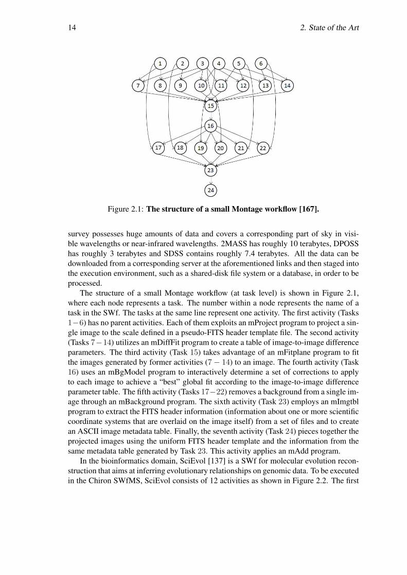
14 2. State of the Art
Figure 2.1: The structure of a small Montage workflow [167].
survey possesses huge amounts of data and covers a corresponding part of sky in visi-ble wavelengths or near-infrared wavelengths. 2MASS has roughly 10 terabytes, DPOSShas roughly 3 terabytes and SDSS contains roughly 7.4 terabytes. All the data can bedownloaded from a corresponding server at the aforementioned links and then staged intothe execution environment, such as a shared-disk file system or a database, in order to beprocessed.
The structure of a small Montage workflow (at task level) is shown in Figure 2.1,where each node represents a task. The number within a node represents the name of atask in the SWf. The tasks at the same line represent one activity. The first activity (Tasks1−6) has no parent activities. Each of them exploits an mProject program to project a sin-gle image to the scale defined in a pseudo-FITS header template file. The second activity(Tasks 7−14) utilizes an mDiffFit program to create a table of image-to-image differenceparameters. The third activity (Task 15) takes advantage of an mFitplane program to fitthe images generated by former activities (7− 14) to an image. The fourth activity (Task16) uses an mBgModel program to interactively determine a set of corrections to applyto each image to achieve a “best” global fit according to the image-to-image differenceparameter table. The fifth activity (Tasks 17−22) removes a background from a single im-age through an mBackground program. The sixth activity (Task 23) employs an mImgtblprogram to extract the FITS header information (information about one or more scientificcoordinate systems that are overlaid on the image itself) from a set of files and to createan ASCII image metadata table. Finally, the seventh activity (Task 24) pieces together theprojected images using the uniform FITS header template and the information from thesame metadata table generated by Task 23. This activity applies an mAdd program.
In the bioinformatics domain, SciEvol [137] is a SWf for molecular evolution recon-struction that aims at inferring evolutionary relationships on genomic data. To be executedin the Chiron SWfMS, SciEvol consists of 12 activities as shown in Figure 2.2. The first

2.2 Scientific Workflow Management 15
Figure 2.2: SciEvol workflow [137].
activity (pre-processing FASTA file) is a Python script to format the multi-fasta inputfile. FASTA file is a textual presenting format for nucleotide or peptide sequences. Thesecond activity (MSA construction) constructs a Multiple Sequence Alignment (MSA)using a MAFFT program (or other MSA programs). A MAFFT program is generally forgenerating the alignment of three or more biological sequences (protein or nucleic acids)of similar length. The third activity (MSA conversion) executes ReadSeq to convert theMSA in FASTA format to that in PHYLIP format, which is used in the phylogenetic treeconstruction activity. The fourth activity (pre-processing PHYLIP file) formats the inputfile (referenced as “phylip-file-one”) according to the format definition and generates asecond file (referenced as “phylip-file-two”). The fifth activity (tree construction) receivesthe “phylip-file-one” as input and produces a phylogenetic tree [72] as output. The sixthactivities (evolutionary analysis from 6.1 to 6.6) analyze the phylogenetic tree with cor-responding parameters and generate a set of files containing evolutionary information asoutput. Each of the activities (evolutionary phases) is related to one of six codon substitu-tion models, which are used to verify if the groups of genes are under positive Darwinianselection. These activities exploit the same program using different parameters. The lastactivity (data analysis) automatically processes the output files obtained from the previousactivities.
There are many other data-intensive SWfs in bioinformatics. For instance, SciPhy-lomics [53] is designed for producing phylogenomic trees based on an input set of pro-tein sequences of genomes to infer evolutionary relationships among living organisms.SciPPGx [63] is a computing and data-intensive pharmacophylogenomic analysis SWffor providing thorough inferring support for pharmacophylogenomic hypotheses. SciPhy[136] is used to construct phylogenetic trees from a set of drug target enzymes found inprotozoan genomes. All these bioinformatics SWfs have been executed using SciCumulus
16 2. State of the Art
SWfMS [51].The components of SWfs can be classified by their functionality, motifs, or structure
patterns. The functionality can be data processing, activity scheduling, activity execution,and resource management [21]. The motifs may be data-oriented and workflow-oriented.Data-oriented motifs consist of recurring activities such as data storage [24], data anal-ysis, data cleaning, data moving [24] and data visualization. Workflow-oriented motifsmay correspond to remote invocations, repetitive activities, parameter sweep workflowsand meta-workflows [24, 78]. A parameter sweep workflow is a workflow with multipleinput parameter sets, which needs to be executed for each input parameter set [41, 87]. Ameta-workflow is a workflow composed of sub-workflows. Workflow structure patternscan be patterns for parallelization, e.g. representing SWfs as algebraic expressions [139],or component structure patterns, e.g. single activity with one or more input/output depen-dencies, sequential control and sequential/concurrent data, synchronization of sequentialdata, data duplication [194]. Moreover, similar structure patterns of SWfs can be foundbased on a similarity model of nodes and edges in the workflow DAG [27]. IdentifyingSWfs or workflow components of the same type enables workflow information sharingand reuse (see Section 2.2.2.2) among workflow designers [194].
2.2.2 Functional Architecture of SWfMSsThe functional architecture of a SWfMS can be layered as follows [60, 201, 21, 139]:presentation, user services, WEP generation, WEP execution and infrastructure. Figure2.3 shows this architecture. The higher layers take advantage of the lower layers to re-alize more concrete functionality. A user interacts with a SWfMS through presentationand realizes the desired functions at user services layer. A SWf is processed at WEPgeneration layer to produce a WEP, which is executed at the WEP execution layer. TheSWfMS accesses the physical resources through the infrastructure layer for SWf execu-tion. The combination of WEP generation layer, WEP execution layer and infrastructurelayer corresponds to a SWf execution engine.
2.2.2.1 Presentation Layer
The presentation layer serves as a User Interface (UI) for the interaction between usersand SWfMSs at all stages of the SWf life cycle. The UI can be textual or graphical.This interface is responsible for designing a SWf by assembling data processing activitieslinked by dependencies. This layer also supports the functionality of showing executionstatus, expressing SWf steering and information sharing commands.
The language for the textual interface is largely used for designing SWfs in SWfMSs.Different from batch scripts, the textual language supports parallel computations on dis-tributed computing and storage resources. The configuration or administration becomescomplicated in this environment while the language defined by a SWfMS should be easyto use. Most SWfMS languages support the specification of a SWf in a DAG structurewhile some SWfMS languages also support iteration for DCG.

2.2 Scientific Workflow Management 17
Figure 2.3: Functional architecture of a SWfMS.
Wilde et al. [188] propose a distributed parallel scripting language called Swift. Swiftsupports SWf specifications in both DAG and DCG. It is a C-like syntax that describesdata, data flows and applications by focusing on concurrent execution, composition andcoordination of independent computational activities. Variables are used in Swift to namethe local variables, arguments, and returns of a function. The variables in Swift havethree types: primitive, mapped, and collection. Primitive variables have the basic datastructures such as integer, float, string, boolean and array. Mapped variables refer to filesexternal to the Swift script. Collection variables are in the structures that contain a set ofvariables, such as arrays. Swift operations have three categories: built-in functions, appli-cation interface functions and compound functions. Built-in functions are implementedby the Swift runtime system to perform various utility functions such as numeric conver-sion, string manipulation, etc. An application interface function provides the informationto the Swift runtime system to invoke a program. A compound function is a function thatinvokes other functions.
Pegasus uses Wings to create SWfs [81]. The SWfs are created through three stagesin Pegasus/Wings: the first stage specifies the abstract structure of the SWf and createsa SWf template; the second stage specifies what data to be used in the SWf and createsa SWf instance; the third stage specifies the data replicas and their locations to form anexecutable SWf. The later stage is done by Pegasus while the first two are realized byWings. In Wings, workflow and its activities are represented as semantic objects. Theprograms are represented as SWf components to process data, which is represented asindividual files or file collections. An activity is represented as a node that contains a
18 2. State of the Art
set of computations, which may contain one computation component or a collection ofcomputations. The data dependencies are represented as links to carry data from or to aSWf node. After the presentation of programs, activities and data dependencies, a SWftemplate is created. With the binding of input data sets, a SWf instance is generated as aDAG in XML format. Then, Pegasus automatically maps the SWf instance to distributedcomputing nodes to form an executable workflow and manages SWf execution.
Chiron [139] also represents the SWfs activities and dependencies as a DAG in XMLtextual format. Ogasawara et al. [138] propose an algebraic language implemented inChiron to encapsulate the SWf activities in six operators: Map, SplitMap, Reduce, Filter,SRQuery and JoinQuery. The Map operator consumes and produces a basic data chunk,which represents the data chunk that has a smallest amount of data while it contains allthe necessary data to be processed in an activity. The SplitMap operator consumes a basicdata chunk while it produces several basic data chunks. The Reduce operator reducesseveral basic data chunks to one basic data chunk. The Filter operator removes uselessdata chunks. SRQuery and MRQuery are traditional relational algebra expressions. Eachactivity corresponds to an operator. These operators are able to parallelize SWf executiononto the distributed computation resources.
Taverna utilizes a simple conceptual unified flow language (Scufl) to represent SWfs[141]. Scufl is an XML-based language, which consists of three main entities: processors,data links, and coordination constraints. Processors represent a computational activity ina SWf. Data links and coordination constraints separately represent the data dependenciesand control dependencies between two activities.
SWfMSs such as Galaxy [82], Taverna [141] and Kepler [21] offer a GUI for SWfdesign. The GUI simplifies the designing process of a SWf for the SWfMS users toassemble the components described as icons through drag-and-drop functionality. Graph-ical SWfMSs combine the efficiency of SWf design and the ease of SWf representation.Desktop-based graphical SWfMSs are typically installed either in a local computer or ina remote server that is accessible through network connection. The local computer orremote server can be connected to large computing and storage resources for large-scaleSWf execution. Some graphical SWfMSs such as Galaxy are web-portal-based, whichmakes it easy to share SWf information among the SWfMS users. With these SWfMSs,a SWf is generally designed in a browser on the client side but executed in a private orpublic web server. Some of the graphical SWfMSs take textual languages as inner repre-sentation of a SWf. For instance, Taverna utilizes Scufl within the SWfMS while Galaxyrepresents workflows in JSON format [16].
2.2.2.2 User Services Layer
The user services layer is responsible for supporting user functionality, i.e. SWf monitor-ing and steering, SWf information sharing and providing SWf provenance data.
SWf monitoring makes it possible to get real-time execution status for SWfMS users.Since SWf execution may take a long time, dynamic monitoring and steering of the exe-cution are important to control SWf execution [57]. SWf monitoring tracks the execution
2.2 Scientific Workflow Management 19
status and displays this information to users during SWf execution [43]. Through SWfmonitoring, a scientist can verify if the result is already enough to prove her hypothesis[46]. SWf monitoring remains an open challenge as it is hard to fully support. How-ever, it can be achieved based on log data (in log files) or more general provenance data,typically in a database [129]. Gunter et al. [89] and Samak et al. [159] propose theStampede monitoring infrastructure for real-time SWf monitoring and troubleshooting.This infrastructure takes a common data model to represent SWf execution and utilizes ahigh-performance loader to normalize the log data. It offers a query interface for extract-ing data from the normalized data. It has been initially integrated with Pegasus SWfMSand then adapted in Triana SWfMS [181]. Horta et al. [95] propose a provenance in-terface to describe the production and consumption relationships between data artifactssuch as output data files and computational activities at runtime for SWf monitoring. Thisinterface can be used to select the desired output data to monitor the SWf execution forSWfMS users through browsers or a high-resolution tiled display. This interface is basedon on-line provenance query supported by algebraic approach. The on-line provenancequery is different from the provenance collected at runtime, but made available only afterthe execution, where monitoring is no longer possible. This interface is available for Ch-iron [139] or SciCumulus [51] that store all the provenance data in a relational database.SciCumulus is an extension of Chiron for cloud environments.
SWf steering is the interaction between a SWfMS and a user to control the work-flow execution progress or configuration parameters [129]. Thus, through SWf steering, ascientist can control SWf execution dynamically so that she does not need to continue un-necessary execution or execute a SWf again when an error occurs [46, 84]. SWf steering,which still remains an open issue, saves much time for SWfMS users.
Information sharing functionality enables SWf information sharing for SWf reusing.Through SWf information sharing, SWfMS users of the same SWfMS environments ordifferent SWfMS environments can share SWf information including SWf design, theinput data or the output data. Since designing a SWf is challenging work, SWf infor-mation sharing is useful to reduce repetitive work between different scientist groups. ASWfMS can directly integrate SWf repositories to support SWf information sharing. ASWf repository is a SWf information pool, where SWf data (input data and output data),SWf designs (structures) and available programs (to be used in activities of workflows)are stored. The SWf repository can contain shared SWfs for the same SWfMS envi-ronments, e.g. “ the myExperiment” social network [191] for Taverna, the web-basedsharing functionality of Galaxy [82], the SWf hosting environment for Askalon [91], orfor different SWfMS environments, e.g. SHIWA Repository [174]. The SWf reposito-ries should support SWf uploading, publishing, download or searching. The SWfs fordifferent SWfMS environments can be adapted to an intermediate representation [151] tocompose a meta-workflow, which can be executed by execution platforms such as SHIWA[175], with corresponding SWfMS engines for the sub-workflows. Except for SHIWA,the information sharing indicates SWf information sharing among the users of the sameSWfMS environment.
Provenance data in SWfs is important to support reproducibility, result interpreta-
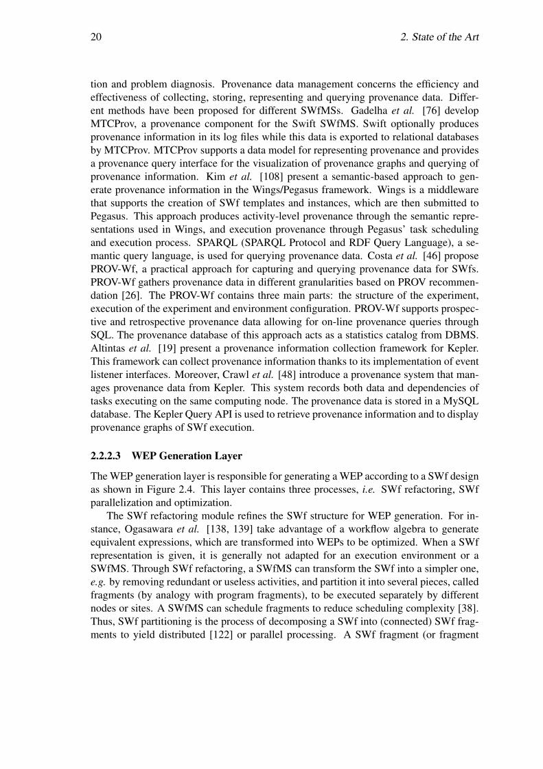
20 2. State of the Art
tion and problem diagnosis. Provenance data management concerns the efficiency andeffectiveness of collecting, storing, representing and querying provenance data. Differ-ent methods have been proposed for different SWfMSs. Gadelha et al. [76] developMTCProv, a provenance component for the Swift SWfMS. Swift optionally producesprovenance information in its log files while this data is exported to relational databasesby MTCProv. MTCProv supports a data model for representing provenance and providesa provenance query interface for the visualization of provenance graphs and querying ofprovenance information. Kim et al. [108] present a semantic-based approach to gen-erate provenance information in the Wings/Pegasus framework. Wings is a middlewarethat supports the creation of SWf templates and instances, which are then submitted toPegasus. This approach produces activity-level provenance through the semantic repre-sentations used in Wings, and execution provenance through Pegasus’ task schedulingand execution process. SPARQL (SPARQL Protocol and RDF Query Language), a se-mantic query language, is used for querying provenance data. Costa et al. [46] proposePROV-Wf, a practical approach for capturing and querying provenance data for SWfs.PROV-Wf gathers provenance data in different granularities based on PROV recommen-dation [26]. The PROV-Wf contains three main parts: the structure of the experiment,execution of the experiment and environment configuration. PROV-Wf supports prospec-tive and retrospective provenance data allowing for on-line provenance queries throughSQL. The provenance database of this approach acts as a statistics catalog from DBMS.Altintas et al. [19] present a provenance information collection framework for Kepler.This framework can collect provenance information thanks to its implementation of eventlistener interfaces. Moreover, Crawl et al. [48] introduce a provenance system that man-ages provenance data from Kepler. This system records both data and dependencies oftasks executing on the same computing node. The provenance data is stored in a MySQLdatabase. The Kepler Query API is used to retrieve provenance information and to displayprovenance graphs of SWf execution.
2.2.2.3 WEP Generation Layer
The WEP generation layer is responsible for generating a WEP according to a SWf designas shown in Figure 2.4. This layer contains three processes, i.e. SWf refactoring, SWfparallelization and optimization.
The SWf refactoring module refines the SWf structure for WEP generation. For in-stance, Ogasawara et al. [138, 139] take advantage of a workflow algebra to generateequivalent expressions, which are transformed into WEPs to be optimized. When a SWfrepresentation is given, it is generally not adapted for an execution environment or aSWfMS. Through SWf refactoring, a SWfMS can transform the SWf into a simpler one,e.g. by removing redundant or useless activities, and partition it into several pieces, calledfragments (by analogy with program fragments), to be executed separately by differentnodes or sites. A SWfMS can schedule fragments to reduce scheduling complexity [38].Thus, SWf partitioning is the process of decomposing a SWf into (connected) SWf frag-ments to yield distributed [122] or parallel processing. A SWf fragment (or fragment
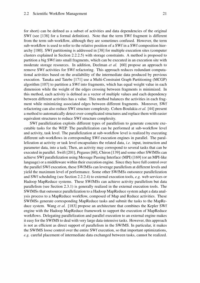
2.2 Scientific Workflow Management 21
for short) can be defined as a subset of activities and data dependencies of the originalSWf (see [138] for a formal definition). Note that the term SWf fragment is differentfrom the term sub-workflow, although they are sometimes confused. However, the termsub-workflow is used to refer to the relative position of a SWf in a SWf composition hier-archy [180]. SWf partitioning is addressed in [38] for multiple execution sites (computerclusters explained in Section 2.2.2.5) with storage constraints. A method is proposed topartition a big SWf into small fragments, which can be executed in an execution site withmoderate storage resources. In addition, Deelman et al. [60] propose an approach toremove SWf activities for SWf refactoring. This approach reduces redundant computa-tional activities based on the availability of the intermediate data produced by previousexecution. Tanaka and Tatebe [171] use a Multi-Constraint Graph Partitioning (MCGP)algorithm [107] to partition a SWf into fragments, which has equal weight value in eachdimension while the weight of the edges crossing between fragments is minimized. Inthis method, each activity is defined as a vector of multiple values and each dependencybetween different activities has a value. This method balances the activities in each frag-ment while minimizing associated edges between different fragments. Moreover, SWfrefactoring can also reduce SWf structure complexity. Cohen-Boulakia et al. [44] presenta method to automatically detect over-complicated structures and replace them with easierequivalent structures to reduce SWf structure complexity.
SWf parallelization exploits different types of parallelism to generate concrete exe-cutable tasks for the WEP. The parallelization can be performed at sub-workflow leveland activity, task level. The parallelization at sub-workflow level is realized by executingdifferent sub-workflows in corresponding SWf execution engines in parallel. The paral-lelization at activity or task level encapsulates the related data, i.e. input, instruction andparameter data, into a task; Then, an activity may correspond to several tasks that can beexecuted in parallel. Swift [201], Pegasus [60], Chiron [139] and some other SWfMSs canachieve SWf parallelization using Message Passing Interface (MPI) [169] (or an MPI-likelanguage) or a middleware within their execution engine. Since they have full control overthe parallel SWf execution, these SWfMSs can leverage parallelism at different levels andyield the maximum level of performance. Some other SWfMSs outsource parallelizationand SWf scheduling (see Section 2.2.2.4) to external execution tools, e.g. web services orHadoop MapReduce systems. These SWfMSs can achieve activity parallelism but dataparallelism (see Section 2.3.1) is generally realized in the external execution tools. TheSWfMSs that outsource parallelization to a Hadoop MapReduce system adapt a data anal-ysis process to a MapReduce workflow, composed of Map and Reduce activities. TheseSWfMSs generate corresponding MapReduce tasks and submit the tasks to the MapRe-duce system. Wang et al. [183] propose an architecture that combines the Kepler SWfengine with the Hadoop MapReduce framework to support the execution of MapReduceworkflows. Delegating parallelization and parallel execution to an external engine makesit easy for the SWfMS to deal with very large data-intensive tasks. However, this approachis not as efficient as direct support of parallelism in the SWfMS. In particular, it makesthe SWfMS loose control over the entire SWf execution, so that important optimizations,e.g. careful placement of intermediate data exchanged between tasks, cannot be realized.
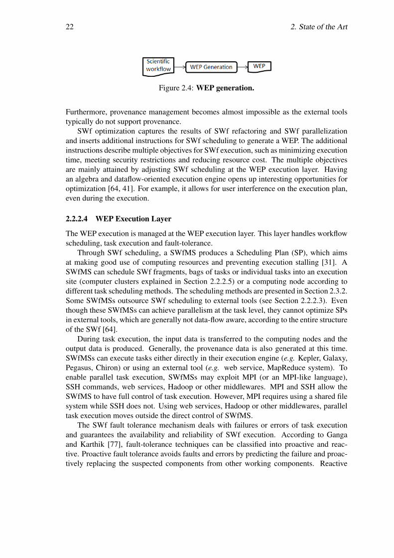
22 2. State of the Art
Figure 2.4: WEP generation.
Furthermore, provenance management becomes almost impossible as the external toolstypically do not support provenance.
SWf optimization captures the results of SWf refactoring and SWf parallelizationand inserts additional instructions for SWf scheduling to generate a WEP. The additionalinstructions describe multiple objectives for SWf execution, such as minimizing executiontime, meeting security restrictions and reducing resource cost. The multiple objectivesare mainly attained by adjusting SWf scheduling at the WEP execution layer. Havingan algebra and dataflow-oriented execution engine opens up interesting opportunities foroptimization [64, 41]. For example, it allows for user interference on the execution plan,even during the execution.
2.2.2.4 WEP Execution Layer
The WEP execution is managed at the WEP execution layer. This layer handles workflowscheduling, task execution and fault-tolerance.
Through SWf scheduling, a SWfMS produces a Scheduling Plan (SP), which aimsat making good use of computing resources and preventing execution stalling [31]. ASWfMS can schedule SWf fragments, bags of tasks or individual tasks into an executionsite (computer clusters explained in Section 2.2.2.5) or a computing node according todifferent task scheduling methods. The scheduling methods are presented in Section 2.3.2.Some SWfMSs outsource SWf scheduling to external tools (see Section 2.2.2.3). Eventhough these SWfMSs can achieve parallelism at the task level, they cannot optimize SPsin external tools, which are generally not data-flow aware, according to the entire structureof the SWf [64].
During task execution, the input data is transferred to the computing nodes and theoutput data is produced. Generally, the provenance data is also generated at this time.SWfMSs can execute tasks either directly in their execution engine (e.g. Kepler, Galaxy,Pegasus, Chiron) or using an external tool (e.g. web service, MapReduce system). Toenable parallel task execution, SWfMSs may exploit MPI (or an MPI-like language),SSH commands, web services, Hadoop or other middlewares. MPI and SSH allow theSWfMS to have full control of task execution. However, MPI requires using a shared filesystem while SSH does not. Using web services, Hadoop or other middlewares, paralleltask execution moves outside the direct control of SWfMS.
The SWf fault tolerance mechanism deals with failures or errors of task executionand guarantees the availability and reliability of SWf execution. According to Gangaand Karthik [77], fault-tolerance techniques can be classified into proactive and reac-tive. Proactive fault tolerance avoids faults and errors by predicting the failure and proac-tively replacing the suspected components from other working components. Reactive
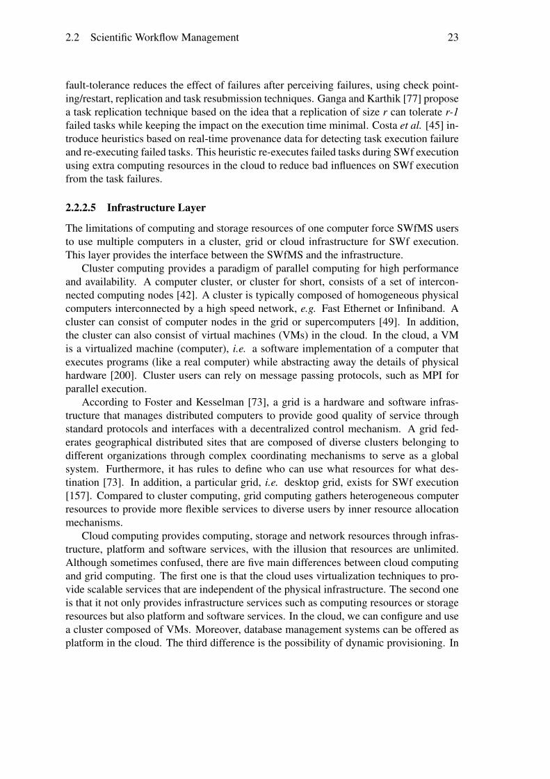
2.2 Scientific Workflow Management 23
fault-tolerance reduces the effect of failures after perceiving failures, using check point-ing/restart, replication and task resubmission techniques. Ganga and Karthik [77] proposea task replication technique based on the idea that a replication of size r can tolerate r-1failed tasks while keeping the impact on the execution time minimal. Costa et al. [45] in-troduce heuristics based on real-time provenance data for detecting task execution failureand re-executing failed tasks. This heuristic re-executes failed tasks during SWf executionusing extra computing resources in the cloud to reduce bad influences on SWf executionfrom the task failures.
2.2.2.5 Infrastructure Layer
The limitations of computing and storage resources of one computer force SWfMS usersto use multiple computers in a cluster, grid or cloud infrastructure for SWf execution.This layer provides the interface between the SWfMS and the infrastructure.
Cluster computing provides a paradigm of parallel computing for high performanceand availability. A computer cluster, or cluster for short, consists of a set of intercon-nected computing nodes [42]. A cluster is typically composed of homogeneous physicalcomputers interconnected by a high speed network, e.g. Fast Ethernet or Infiniband. Acluster can consist of computer nodes in the grid or supercomputers [49]. In addition,the cluster can also consist of virtual machines (VMs) in the cloud. In the cloud, a VMis a virtualized machine (computer), i.e. a software implementation of a computer thatexecutes programs (like a real computer) while abstracting away the details of physicalhardware [200]. Cluster users can rely on message passing protocols, such as MPI forparallel execution.
According to Foster and Kesselman [73], a grid is a hardware and software infras-tructure that manages distributed computers to provide good quality of service throughstandard protocols and interfaces with a decentralized control mechanism. A grid fed-erates geographical distributed sites that are composed of diverse clusters belonging todifferent organizations through complex coordinating mechanisms to serve as a globalsystem. Furthermore, it has rules to define who can use what resources for what des-tination [73]. In addition, a particular grid, i.e. desktop grid, exists for SWf execution[157]. Compared to cluster computing, grid computing gathers heterogeneous computerresources to provide more flexible services to diverse users by inner resource allocationmechanisms.
Cloud computing provides computing, storage and network resources through infras-tructure, platform and software services, with the illusion that resources are unlimited.Although sometimes confused, there are five main differences between cloud computingand grid computing. The first one is that the cloud uses virtualization techniques to pro-vide scalable services that are independent of the physical infrastructure. The second oneis that it not only provides infrastructure services such as computing resources or storageresources but also platform and software services. In the cloud, we can configure and usea cluster composed of VMs. Moreover, database management systems can be offered asplatform in the cloud. The third difference is the possibility of dynamic provisioning. In

24 2. State of the Art
a grid environment, a list of resources is generally fixed during the entire execution ofthe SWf. Thus, it is very unusual to use dynamic provisioning in the grid as it does notprovide any benefit. In contrast, in cloud environments, we have a list of resource typesfrom which we can provision a potentially unlimited number of resource instances. Suchdynamic provisioning can provide much more benefits, in particular better performance,and reduced financial cost. The fourth difference is in the use of service-level agree-ment (SLA), which defines the quality of service provided to users by service providers[187]. Cloud SLA includes relatively full performance metrics for on-demand services[32] while grid SLA is relatively informal. The fifth difference is that the cloud providessupport for pricing and accounting services, which is not necessary in the grid. Somegrids evolve towards the cloud. For instance, Grid’5000 [13] is a grid in France whichprovides virtualized resources and services for big data (e.g. Hadoop).
The operational layer is also in charge of provisioning, which can be static or dy-namic. Static provisioning can provide unchangeable resources for SWfMSs during SWfexecution while dynamic provisioning can add or remove resources for SWfMSs at run-time. Based on the types of resources, provisioning can be classified into computing pro-visioning and storage provisioning. Computing provisioning means offering computingnodes to SWfMSs while storage provisioning means providing storage resources for datacaching or data persistence. However, most SWfMSs are just adapted to static computingand storage provisioning.
The data storage module generally exploit database management systems and file sys-tems to manage the data during SWf execution. Some SWfMSs such as Taverna putintermediate data and output data in a database. As proposed in [202], some SWfMSssuch as Pegasus and Chiron utilize a shared-disk file system (see Section 2.4.3.1). SomeSWfMSs such as Kepler [183] can exploit distributed file systems (see Section 2.4.3.1).Some SWfMSs such as Pegasus can directly take advantage of the local file systems ineach computing node. Generally, the file systems and the database management systemstake advantage of computing nodes and storage resources provided by the provisioningmodule. In a multisite environment, SWfMSs can cluster the data and place each data setat a single site, distribute the newly generated data to multiple sites at runtime and adjustdata among multiple sites [197]. SWfMSs can also put some data in the disk cache of onecomputing node to accelerate data access during SWf execution [165]. However, existingSWfMSs just use few types of storage resources, some other types of storage resources,e.g. cache for a single site, cache in one computing node etc., can be also exploited.
2.2.3 Techniques for Data-intensive Scientific WorkflowsBecause they deal with big data, data-intensive SWfs have some features that make themmore complicated to handle, compared with traditional SWfs. From the existing solutions,we can observe three main features, which we briefly discuss.
The first feature is the diversity of data sources and data formats in data-intensiveSWfs. The data can consist of the input data stored in a shared-disk file system and theintermediate data stored in a database. The data of various data sources differ in data
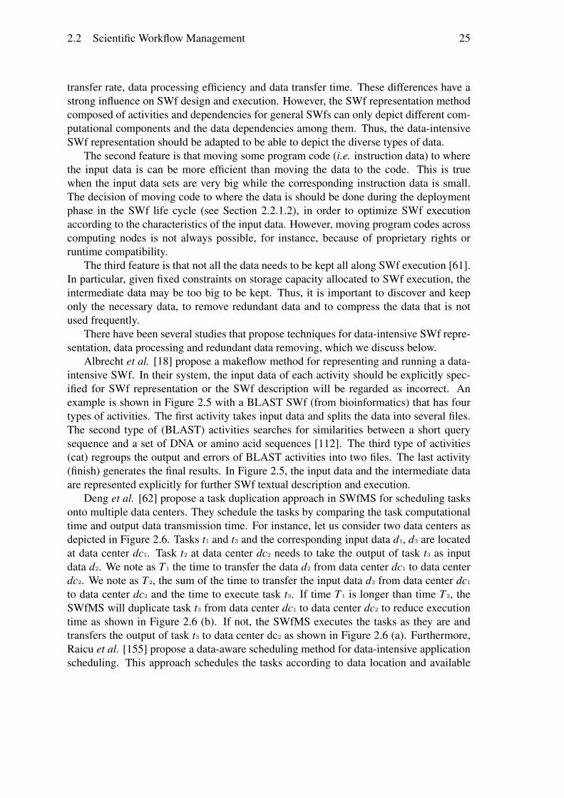
2.2 Scientific Workflow Management 25
transfer rate, data processing efficiency and data transfer time. These differences have astrong influence on SWf design and execution. However, the SWf representation methodcomposed of activities and dependencies for general SWfs can only depict different com-putational components and the data dependencies among them. Thus, the data-intensiveSWf representation should be adapted to be able to depict the diverse types of data.
The second feature is that moving some program code (i.e. instruction data) to wherethe input data is can be more efficient than moving the data to the code. This is truewhen the input data sets are very big while the corresponding instruction data is small.The decision of moving code to where the data is should be done during the deploymentphase in the SWf life cycle (see Section 2.2.1.2), in order to optimize SWf executionaccording to the characteristics of the input data. However, moving program codes acrosscomputing nodes is not always possible, for instance, because of proprietary rights orruntime compatibility.
The third feature is that not all the data needs to be kept all along SWf execution [61].In particular, given fixed constraints on storage capacity allocated to SWf execution, theintermediate data may be too big to be kept. Thus, it is important to discover and keeponly the necessary data, to remove redundant data and to compress the data that is notused frequently.
There have been several studies that propose techniques for data-intensive SWf repre-sentation, data processing and redundant data removing, which we discuss below.
Albrecht et al. [18] propose a makeflow method for representing and running a data-intensive SWf. In their system, the input data of each activity should be explicitly spec-ified for SWf representation or the SWf description will be regarded as incorrect. Anexample is shown in Figure 2.5 with a BLAST SWf (from bioinformatics) that has fourtypes of activities. The first activity takes input data and splits the data into several files.The second type of (BLAST) activities searches for similarities between a short querysequence and a set of DNA or amino acid sequences [112]. The third type of activities(cat) regroups the output and errors of BLAST activities into two files. The last activity(finish) generates the final results. In Figure 2.5, the input data and the intermediate dataare represented explicitly for further SWf textual description and execution.
Deng et al. [62] propose a task duplication approach in SWfMS for scheduling tasksonto multiple data centers. They schedule the tasks by comparing the task computationaltime and output data transmission time. For instance, let us consider two data centers asdepicted in Figure 2.6. Tasks t1 and t3 and the corresponding input data d1, d3 are locatedat data center dc1. Task t2 at data center dc2 needs to take the output of task t3 as inputdata d2. We note as T1 the time to transfer the data d2 from data center dc1 to data centerdc2. We note as T2, the sum of the time to transfer the input data d3 from data center dc1
to data center dc2 and the time to execute task t3. If time T1 is longer than time T2, theSWfMS will duplicate task t3 from data center dc1 to data center dc2 to reduce executiontime as shown in Figure 2.6 (b). If not, the SWfMS executes the tasks as they are andtransfers the output of task t3 to data center dc2 as shown in Figure 2.6 (a). Furthermore,Raicu et al. [155] propose a data-aware scheduling method for data-intensive applicationscheduling. This approach schedules the tasks according to data location and available

26 2. State of the Art
Figure 2.5: BLAST SWf [18].
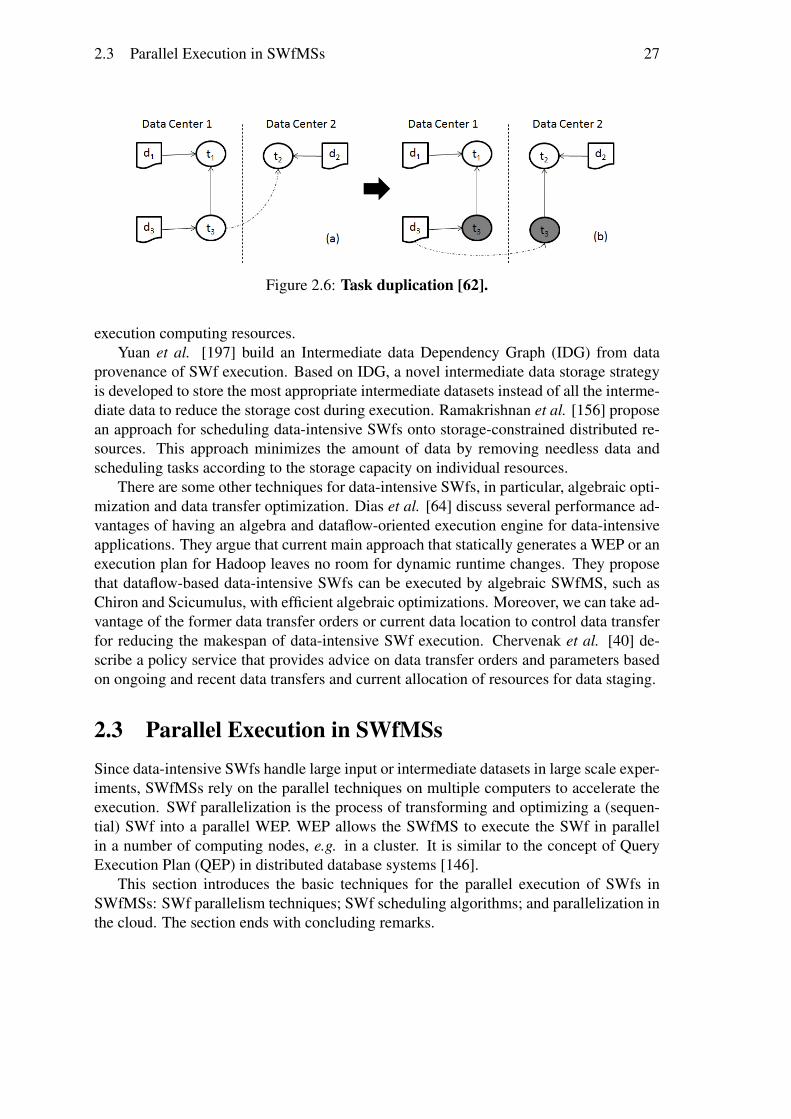
2.3 Parallel Execution in SWfMSs 27
Figure 2.6: Task duplication [62].
execution computing resources.Yuan et al. [197] build an Intermediate data Dependency Graph (IDG) from data
provenance of SWf execution. Based on IDG, a novel intermediate data storage strategyis developed to store the most appropriate intermediate datasets instead of all the interme-diate data to reduce the storage cost during execution. Ramakrishnan et al. [156] proposean approach for scheduling data-intensive SWfs onto storage-constrained distributed re-sources. This approach minimizes the amount of data by removing needless data andscheduling tasks according to the storage capacity on individual resources.
There are some other techniques for data-intensive SWfs, in particular, algebraic opti-mization and data transfer optimization. Dias et al. [64] discuss several performance ad-vantages of having an algebra and dataflow-oriented execution engine for data-intensiveapplications. They argue that current main approach that statically generates a WEP or anexecution plan for Hadoop leaves no room for dynamic runtime changes. They proposethat dataflow-based data-intensive SWfs can be executed by algebraic SWfMS, such asChiron and Scicumulus, with efficient algebraic optimizations. Moreover, we can take ad-vantage of the former data transfer orders or current data location to control data transferfor reducing the makespan of data-intensive SWf execution. Chervenak et al. [40] de-scribe a policy service that provides advice on data transfer orders and parameters basedon ongoing and recent data transfers and current allocation of resources for data staging.
2.3 Parallel Execution in SWfMSsSince data-intensive SWfs handle large input or intermediate datasets in large scale exper-iments, SWfMSs rely on the parallel techniques on multiple computers to accelerate theexecution. SWf parallelization is the process of transforming and optimizing a (sequen-tial) SWf into a parallel WEP. WEP allows the SWfMS to execute the SWf in parallelin a number of computing nodes, e.g. in a cluster. It is similar to the concept of QueryExecution Plan (QEP) in distributed database systems [146].
This section introduces the basic techniques for the parallel execution of SWfs inSWfMSs: SWf parallelism techniques; SWf scheduling algorithms; and parallelization inthe cloud. The section ends with concluding remarks.
28 2. State of the Art
2.3.1 Scientific Workflow ParallelismSWf parallelization identifies the tasks that can be executed in parallel in the WEP. Similarto parallel query processing [146], whereby a QEP can be parallelized based on data andoperator dependencies. There are two parallelism levels: coarse-grained parallelism andfine-grained parallelism. Coarse-grained parallelism can achieve parallelism by executingsub-workflows or fragments in parallel. Fine-grained parallelism realizes parallelism byexecuting different activities in parallel. If a SWf is composed of sub-workflows, it can beexecuted in parallel at coarse-grained level to parallelize the execution of sub-workflowsand then, executed in parallel at fine-grained level to parallelize the execution of activitieswithin sub-workflows. If a SWf is directly composed of activities, it can just be executedat fine-grained parallelism level to parallelize the execution of activities.
According to the dependencies defined in a SWf, different parallelization techniquescan result in various execution plans. Some parameters can be used to evaluate the ef-ficiency of each technique. An important parameter of parallelization is the degree ofparallelism, which is defined as the number of concurrently running computing nodes orthreads at any given time and that can vary for a given SWf depending on the type ofparallelism [33].
2.3.1.1 Coarse-Grained Parallelism
Coarse-grained parallelism is performed at workflow level, which is critical to the exe-cution of meta-workflows or parameter sweep workflows. To execute a meta-workflow,the independent sub-workflows are identified as SWf fragments to be submitted to cor-responding SWf execution engine [174]. The execution of a parameter sweep SWf cor-responds to the execution of the SWf with different sets of input parameter values. Thecombination of SWf and each set of input parameter values is viewed as independentsub-workflows, which can be run in parallel [104]. In addition, a SWf can achieve coarse-grained parallelism by SWf partitioning. The coarse-grained parallelism for parallel ex-ecution of sub-workflows resembles to the independent activity parallelism presented inthe next section.
2.3.1.2 Fine-Grained Parallelism
The fine-grained parallelism is realized within a SWf, a sub-workflow (for meta-workflows)or a SWf fragment. Three types of parallelism exist at this level: data parallelism, inde-pendent parallelism and pipeline parallelism. Data parallelism deals with the parallelismwithin an activity while independent parallelism and pipeline parallelism handle the par-allelism between different activities.
Data Parallelism
Data parallelism, similar to intra-operator parallelism in [146], is obtained by having mul-tiple tasks performing the same activity, each on a different data chunk. As shown in Fig-
2.3 Parallel Execution in SWfMSs 29
ure 2.7(b), data parallelism happens when the input data of an activity can be partitionedinto different chunks and each chunk is processed independently by a task in a differentcomputing node or processor. As the input data needs be partitioned, e.g. by a partition-ing task, the activity result is also partitioned. Thus, the partitioned output data can be thebase for data parallelism for the next activities. However, to combine the different resultsto produce a single result, e.g. the final result to be delivered to the user, requires specialprocessing, e.g. by having all the tasks writing to a shared disk or sending their results toa task that produces the single result.
Data parallelism can be static, dynamic or adaptive [148]. If the number of datachunks is indicated before execution and fixed during execution, the data parallelism isstatic. If the number of data chunks is determined at run-time, the data parallelism is dy-namic. In addition, if the number is automatically adapted to the execution environment,the data parallelism is adaptive. The adaptive data parallelism can determine the bestnumber of data chunks to balance SWf execution, to increase parallelism degree whilemaintaining a reasonable overhead.
Independent Parallelism
Different activities of a SWf can be executed in parallel over several computing nodes.Two activities can be either independent, i.e. the execution of any activity does not dependon the output data of the other one, or dependent, i.e. there is a data dependency betweenthem. Independent parallelism exploits independent activities while pipeline parallelism(see next subsection) deals with dependent activities.
Independent parallelism is achieved by having tasks of different independent activi-ties executed simultaneously. As shown in Figure 2.7(c), independent parallelism occurswhen a SWf has more than one independent part in the graph and the activities in eachpart have no data dependencies with those in another part. To achieve independent par-allelism, a SWfMS should identify activities that can be executed in parallel. SWfMSscan partition the SWf into independent parts (or SWf fragments) of activities to achieveindependent parallelism.
Pipeline Parallelism
With pipeline parallelism (see Figure 2.7(d)), several dependent activities with a producer-consumer relationship are executed in parallel by different tasks. One output data chunkof one activity is consumed directly by the next dependent activities in a pipeline fashion.The advantage of pipeline execution is that the result of the producer activity does notneed to be entirely materialized. Instead, data chunks can be consumed as soon as theyare ready, thus saving memory and disk accesses.
Hybrid Parallelism
As shown in Figure 2.7(e), the three basic types of parallelism can be combined to achievehigher degrees of parallelism. A SWfMS can first perform data parallelism within each

30 2. State of the Art
(a) Sequential execution in one computing node. Activity B starts execution after theexecution of activity A and activity C starts execution after the execution of activity B. Allthe execution is realized in one computing node.
(b) Data parallelism. The execution of activities A, B, C is performed in two computingnodes simultaneously. Each computing node processes a data chunk.
(c) Independent parallelism. The execution of activities A and B is performed in two com-puting nodes simultaneously. Activity C begins execution after the execution of activities Aand B.
(d) Pipeline parallelism. Activity C starts execution once a data chunk is ready. Whenactivities A and B are processing the second part of data (i2, i4), activity C can process theoutput data of the first part (a1, b1) at the same time.
(e) Hybrid parallelism. Activity A is executed through data parallelism at nodes 1 and 2.Activity B is executed through data parallelism at nodes 4 and 5. Activities A and B are alsoexecuted through independent parallelism. Activities A and C, respectively B and C, areexecuted through pipeline parallelism between nodes (1, 2) and 3, respectively nodes (4, 5)and 3.
Figure 2.7: Different types of parallelism. Circles represent activities. There are threeactivities: A, B and C. C processes the output data produced by A and B. Rectangles rep-resent data chunks. “i1” stands for the first part of input data. “a1” stands for the outputdata corresponding to the first part of input data after being processed by activity A.
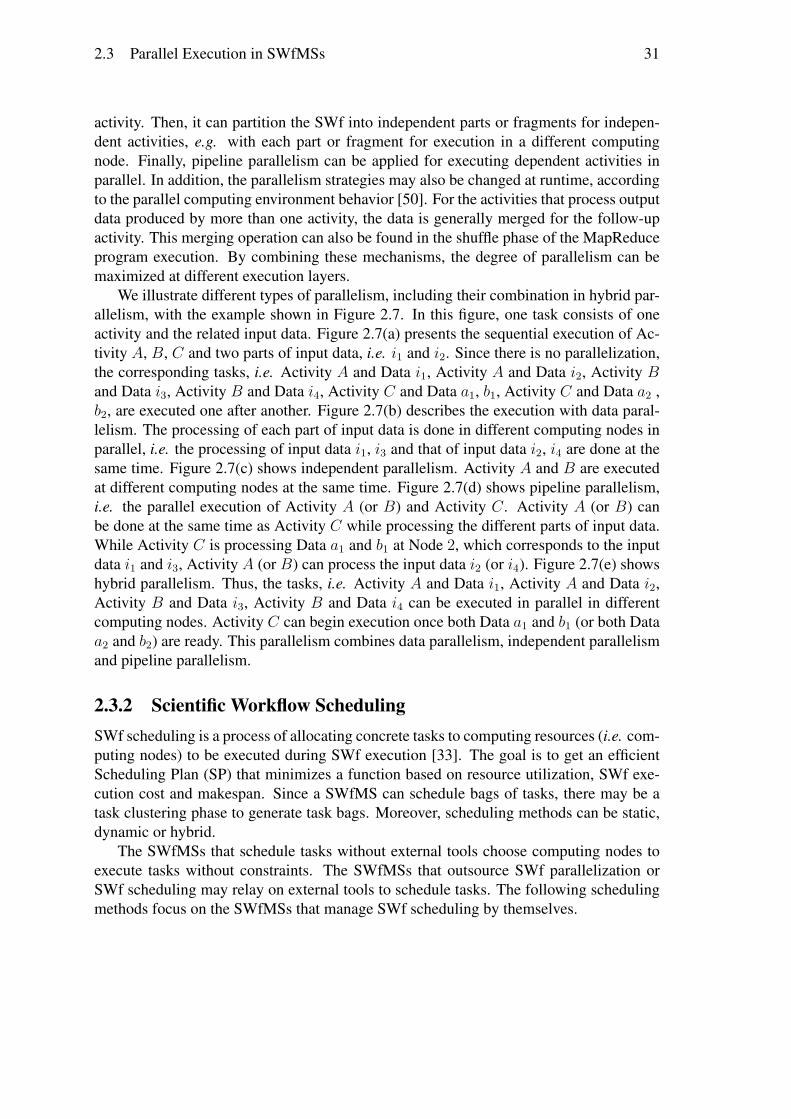
2.3 Parallel Execution in SWfMSs 31
activity. Then, it can partition the SWf into independent parts or fragments for indepen-dent activities, e.g. with each part or fragment for execution in a different computingnode. Finally, pipeline parallelism can be applied for executing dependent activities inparallel. In addition, the parallelism strategies may also be changed at runtime, accordingto the parallel computing environment behavior [50]. For the activities that process outputdata produced by more than one activity, the data is generally merged for the follow-upactivity. This merging operation can also be found in the shuffle phase of the MapReduceprogram execution. By combining these mechanisms, the degree of parallelism can bemaximized at different execution layers.
We illustrate different types of parallelism, including their combination in hybrid par-allelism, with the example shown in Figure 2.7. In this figure, one task consists of oneactivity and the related input data. Figure 2.7(a) presents the sequential execution of Ac-tivity A, B, C and two parts of input data, i.e. i1 and i2. Since there is no parallelization,the corresponding tasks, i.e. Activity A and Data i1, Activity A and Data i2, Activity Band Data i3, Activity B and Data i4, Activity C and Data a1, b1, Activity C and Data a2 ,b2, are executed one after another. Figure 2.7(b) describes the execution with data paral-lelism. The processing of each part of input data is done in different computing nodes inparallel, i.e. the processing of input data i1, i3 and that of input data i2, i4 are done at thesame time. Figure 2.7(c) shows independent parallelism. Activity A and B are executedat different computing nodes at the same time. Figure 2.7(d) shows pipeline parallelism,i.e. the parallel execution of Activity A (or B) and Activity C. Activity A (or B) canbe done at the same time as Activity C while processing the different parts of input data.While Activity C is processing Data a1 and b1 at Node 2, which corresponds to the inputdata i1 and i3, Activity A (or B) can process the input data i2 (or i4). Figure 2.7(e) showshybrid parallelism. Thus, the tasks, i.e. Activity A and Data i1, Activity A and Data i2,Activity B and Data i3, Activity B and Data i4 can be executed in parallel in differentcomputing nodes. Activity C can begin execution once both Data a1 and b1 (or both Dataa2 and b2) are ready. This parallelism combines data parallelism, independent parallelismand pipeline parallelism.
2.3.2 Scientific Workflow SchedulingSWf scheduling is a process of allocating concrete tasks to computing resources (i.e. com-puting nodes) to be executed during SWf execution [33]. The goal is to get an efficientScheduling Plan (SP) that minimizes a function based on resource utilization, SWf exe-cution cost and makespan. Since a SWfMS can schedule bags of tasks, there may be atask clustering phase to generate task bags. Moreover, scheduling methods can be static,dynamic or hybrid.
The SWfMSs that schedule tasks without external tools choose computing nodes toexecute tasks without constraints. The SWfMSs that outsource SWf parallelization orSWf scheduling may relay on external tools to schedule tasks. The following schedulingmethods focus on the SWfMSs that manage SWf scheduling by themselves.
32 2. State of the Art
2.3.2.1 Task Clustering
A SWfMS can schedule bags of tasks to a computing nodes or multiple computing nodesto reduce the scheduling overhead so that the execution time can be reduced. A bag oftasks contains several tasks to be executed in the same computing node. Note that bags oftasks are different from fragments. Fragments are generated by analyzing activities whilebags of tasks are produced by grouping executable tasks. Several studies have been donefor generating bags of tasks. Deng et al. [62] present a clustering method for efficientSWf execution. They use a k-means clustering method to group the tasks into several taskbags according to different dependencies: data-data dependency, task-task dependency,and task-data dependency. These three types of dependencies are used to measure thecorrelations between datasets and tasks in a SWf. W. Chen et al. [39] present a balancedtask clustering approach for SWf execution. They cluster the tasks by balancing totalexecution of each bag of task.
2.3.2.2 Static Scheduling
Static scheduling generates a SP that allocates all the executable tasks to computing nodesbefore execution and the SWfMS strictly abides the SP during the whole SWf execution[33]. Because it is before execution, static scheduling yields little overhead at runtime. Itis efficient if the SWfMS can predict the execution load of each task accurately, when theexecution environment varies little during the SWf execution, and when the SWfMS hasenough information about the computing and storage capabilities of the correspondingcomputers. However, when the execution environment experiences dynamical changes, itis very difficult to achieve load balance. The static task scheduling algorithms have twokinds of processor selection methods [177]: heuristic-based and guided random searchbased. The heuristic-based method schedules tasks according to a predefined rule whilethe random search based method schedules tasks randomly. Static task scheduling al-gorithms can also be classified between task-based and workflow-based [30]. The task-based method directly schedules tasks into computing nodes while the workflow-basedmethod schedules a fragment into computing nodes. Since the workflow-based methodtransfers the data with less overhead compared to the task-based method, it is better fordata-intensive applications.
Topcuouglu et al. [177] propose two static scheduling algorithms: HeterogeneousEarliest-Finish-Time (HEFT) and Critical-Path-on-a-Processor (CPOP). Both algorithmscontain a task prioritizing phase and a processor selection phase. The task prioritizingphase is for ranking tasks while the processor selection phase is for scheduling a selectedtask on a “best” computing node, which minimizes the total execution time. We note theaverage computation cost of a task as CPC and the average communication cost of thecurrent task to a succeed task as CMC. The ranku is the rank that is based on CPC andCMC. The rankd indicates the rank based on CPC and CMC consisting of the commu-nication from a preceding task to the current task. In the task prioritizing phase, HEFTranks tasks based on ranku. In the processor selection phase, HEFT selects a computingnode, which finishes its current task firsts. HEFT can also insert a task in a computing
2.3 Parallel Execution in SWfMSs 33
node when there is idle time between the execution of two consecutive tasks. The CPOPalgorithm uses a rankc that combines both ranku and rankd in the task prioritizing phase.It utilizes a critical path in the processor selection phase. A critical path is a pipeline oftasks, in which a task has no more than one input dependency and no more than one outputdependency. Each task in the critical path has the highest priority value (in rankc) in allthe tasks that have the input data dependencies from the same parent task. CPOP choosesa computing node as a critical-path processor and schedules the tasks in the critical pathto the critical-path processor. It schedules the other tasks to the other computing nodeswith the same mechanism as HEFT.
2.3.2.3 Dynamic Scheduling
Dynamic scheduling produces SPs that distribute and allocate executable tasks to comput-ing nodes during SWf execution [33]. This kind of scheduling is appropriate for SWfs, inwhich the workload of tasks is difficult to estimate, or for environments where the capabil-ities of the computers varies a lot during execution. Dynamic scheduling can achieve loadbalancing while it takes time to dynamically generate SPs during execution. The schedul-ing algorithms can be based on the queue techniques in a publish/subscribe model withdifferent strategies such as First In First Out (FIFO), adaptive and so on. SWfMSs suchas Swift [188], Chiron [139], and Galaxy [106] exploit dynamic scheduling algorithms.
Dynamic SPs may be generated by adapting a static scheduling method to dynamicenvironment. Yu and Shi [196] introduce an HEFT-based dynamic scheduling algorithm.This algorithm is suited to the situation where a SWf has been executed partially beforescheduling. It schedules the tasks by applying an HEFT-based algorithm according to adynamically generated rank of tasks.
There are some original approaches to generate dynamic SPs. Maheswaran et al.[125] present a min-min algorithm that is designed as a batch mode scheduling of twosteps. First, a list of tasks ready to be executed is created. This phase is called “taskprioritizing” phase. Then, the tasks in the list are scheduled to computing nodes basedon a heuristic. The heuristic maps the task T to the computing node M such that T is thetask that has minimum expected execution time in the non-mapped tasks and that M is thecomputing node that is executing a task having minimum expected execution time in themapped tasks. This phase is called the “resource selection” phase.
Anglano and Canonico [22] present several knowledge-free scheduling algorithmsthat are able to schedule multiple bags of tasks. A knowledge-free algorithm does notrequire any information on the resources for scheduling. These algorithms implementdifferent policies: First Come First Served – Exclusive (FCFS-Excl), First Come FirstServed – Shared (FCFS-Share), Round Robin (RR), Round Robin –No Replica First (RR-NRF) and Longest Idle. With the FCFS-Excl policy, bags of tasks are scheduled in orderof arrival. Different from FCFS-Excl, FCFS-Share can allocate more than one bag oftasks to a computing node. The RR policy schedules bags of tasks in a fixed circularorder while all the bags have the same probability to be scheduled. With the RR-NRFpolicy, a bag of tasks that does not have any task executed will be given priority. In this

34 2. State of the Art
policy, all the bags of tasks have at least a task running. The longest idle policy tries toreduce waiting time by giving preference to the bag of tasks hosting the task that exhibitsthe largest waiting time. The paper shows that the FCFS-based policy performs better forsmall task granularity scheduling.
2.3.2.4 Hybrid Scheduling
Both of static and dynamic scheduling have their own advantages and they can be com-bined as a hybrid scheduling method to achieve better performance than just using oneor the other. For example, a SWfMS might schedule a part of the tasks of a SWf, e.g.those tasks for which there is enough information, using static scheduling and schedulethe other part during execution with dynamic scheduling [62].
Oliveira et al. [50] propose a hybrid scheduling method with several algorithms:greedy scheduling, task grouping, task performing, and load balancing. The greedyscheduling algorithm produces static WEPs to choose the most suitable task to executefor a given idle VM based on a proposed cost model. The task grouping algorithm pro-duces new tasks by encapsulating two or more tasks into a new one. The task performingalgorithm sets up the granularity factor for each VM in the system and modifies the granu-larity according to the average execution time. The load balancing algorithm is a dynamicscheduling algorithm that adjusts the number of VMs and static WEP in order to meet thedeadline of execution time and the budget limit.
2.3.2.5 Scheduling Optimization Algorithms
Since there are many criteria to measure SWf execution, SWfMS users may have multipleobjectives for SWf execution, such as reducing execution time, minimizing monetary costetc. Therefore, SPs should also be optimized to attain multiple objective in a given context(cluster, grid, cloud). Unlike query optimization in database, however, this optimizationphase is often not explicit and mixed with the scheduling method. Though there aresome existing scheduling optimization algorithms [50, 88, 70, 65], they do not considera multisite environment with distributed data at each site. We present [88] and [70] asexamples.
Gu et al. [88] address the scheduling optimization problem of mapping distributedSWf to maximize the throughput in unstable networks where nodes and links are sub-ject to probabilistic failures. And they propose a mapping algorithm to maximize boththroughput and reliability for SWf scheduling. They consider a network where the failureoccurrences follow a Poisson distribution with a constant parameter. The mapping algo-rithm includes three algorithms: disLDP-F, Greedy disLDP-F and decentralized GreedydisLDP-F. The disLDP-F algorithm schedules the tasks by identifying and minimizing theglobal bottleneck time based on the rank of computational requirements of tasks. GreedydisLDP-F reduces the search complexity of disLDP-F by selecting the best node for eachtype of requirement of the current task and then generates a best computing node for thecurrent task. The decentralized Greedy disLDP-F algorithm decentralizes the disLDP-F
2.4 SWfMS in a Multisite Cloud 35
algorithm by storing all the parameters of each individual node locally and selecting thenode through the communication between individual nodes instead of centralized control.
Fard et al. [70] propose a multi-objective scheduling method of SWf execution in dis-tributed computing infrastructures. Their approach generates a best scheduling strategy,which is a Pareto optimality (no other strategy can achieve a result of a better componentwhile ensuring the other components of the result as well as this strategy), to achieve 4objectives, i.e. execution time, monetary cost, energy consumption and reliability. Nev-ertheless, this approach does not consider data distribution in a multisite environment.
2.3.2.6 Conclusion
Data-intensive SWfs need to process big data, which may take a very long time with se-quential execution. Parallel execution is therefore necessary to reduce execution time onparallel computers. SWf parallel execution exploits a WEP that includes parallel execu-tion decisions, which achieves SWf parallelism. The parallel execution also schedulesexecution tasks to computing nodes with optimization instructions.
SWf parallelism consists of two lelvels, i.e. fine-grained and coarse-grained. Fine-grained parallelism is for parallelizing the execution of sub-workflows and fragments.Coarse-grained parallelism parallelizes the execution of activities in three basic types:data parallelism, independent parallelism and pipeline parallelism. Data parallelism isfine-grained parallelism within one activity and can yield a very high degree of parallelismon big datasets. Independent parallelism and pipeline parallelism exploit the parallelismbetween different activities. These are coarse-grained and the degree of parallelism isbound by the maximum of activities. Therefore, the highest levels of parallelism can beachieved by combining these three types of parallelism into hybrid parallelism.
SWf scheduling is a process of allocating concrete tasks to computing node duringSWf execution. Static scheduling method generates a SP prior to SWf execution and thusSWf execution is very fast, but it makes SWfMSs difficult to achieve load balancing at adynamically changing environment. Dynamic scheduling can better achieve load balanc-ing but takes more time to generate SPs at run-time. Hybrid scheduling can combine thebest of both static and dynamic scheduling. SWf scheduling performs some optimization,trying to reach multiple objectives such as minimizing the makespan of SWf execution orreducing monetary expenses.
2.4 SWfMS in a Multisite CloudThe cloud, which provides virtually infinite computing and storage resources, appears asa cost-effective solution to deploy and to run data-intensive SWfs. For scalability andhigh availability, large cloud providers such as Amazon and Microsoft typically havemultiple data centers located at different sites. In general, a user uses a single site, whichis sufficient for most applications. However, there are important cases where SWfs willneed to be deployed at several sites, e.g. because the data accessed by the SWf is indifferent research groups’ databases at different sites or because SWf execution needs
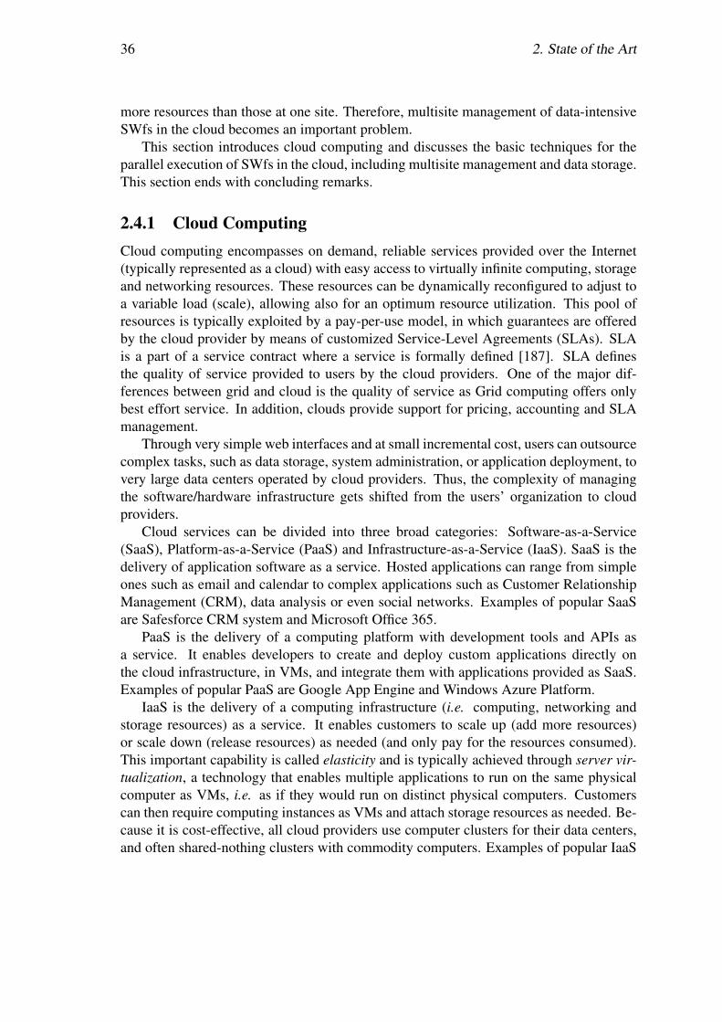
36 2. State of the Art
more resources than those at one site. Therefore, multisite management of data-intensiveSWfs in the cloud becomes an important problem.
This section introduces cloud computing and discusses the basic techniques for theparallel execution of SWfs in the cloud, including multisite management and data storage.This section ends with concluding remarks.
2.4.1 Cloud ComputingCloud computing encompasses on demand, reliable services provided over the Internet(typically represented as a cloud) with easy access to virtually infinite computing, storageand networking resources. These resources can be dynamically reconfigured to adjust toa variable load (scale), allowing also for an optimum resource utilization. This pool ofresources is typically exploited by a pay-per-use model, in which guarantees are offeredby the cloud provider by means of customized Service-Level Agreements (SLAs). SLAis a part of a service contract where a service is formally defined [187]. SLA definesthe quality of service provided to users by the cloud providers. One of the major dif-ferences between grid and cloud is the quality of service as Grid computing offers onlybest effort service. In addition, clouds provide support for pricing, accounting and SLAmanagement.
Through very simple web interfaces and at small incremental cost, users can outsourcecomplex tasks, such as data storage, system administration, or application deployment, tovery large data centers operated by cloud providers. Thus, the complexity of managingthe software/hardware infrastructure gets shifted from the users’ organization to cloudproviders.
Cloud services can be divided into three broad categories: Software-as-a-Service(SaaS), Platform-as-a-Service (PaaS) and Infrastructure-as-a-Service (IaaS). SaaS is thedelivery of application software as a service. Hosted applications can range from simpleones such as email and calendar to complex applications such as Customer RelationshipManagement (CRM), data analysis or even social networks. Examples of popular SaaSare Safesforce CRM system and Microsoft Office 365.
PaaS is the delivery of a computing platform with development tools and APIs asa service. It enables developers to create and deploy custom applications directly onthe cloud infrastructure, in VMs, and integrate them with applications provided as SaaS.Examples of popular PaaS are Google App Engine and Windows Azure Platform.
IaaS is the delivery of a computing infrastructure (i.e. computing, networking andstorage resources) as a service. It enables customers to scale up (add more resources)or scale down (release resources) as needed (and only pay for the resources consumed).This important capability is called elasticity and is typically achieved through server vir-tualization, a technology that enables multiple applications to run on the same physicalcomputer as VMs, i.e. as if they would run on distinct physical computers. Customerscan then require computing instances as VMs and attach storage resources as needed. Be-cause it is cost-effective, all cloud providers use computer clusters for their data centers,and often shared-nothing clusters with commodity computers. Examples of popular IaaS
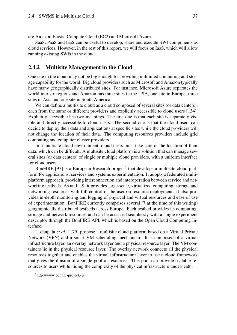
2.4 SWfMS in a Multisite Cloud 37
are Amazon Elastic Compute Cloud (EC2) and Microsoft Azure.SaaS, PaaS and IaaS can be useful to develop, share and execute SWf components as
cloud services. However, in the rest of this report, we will focus on IaaS, which will allowrunning existing SWfs in the cloud.
2.4.2 Multisite Management in the CloudOne site in the cloud may not be big enough for providing unlimited computing and stor-age capability for the world. Big cloud providers such as Microsoft and Amazon typicallyhave many geographically distributed sites. For instance, Microsoft Azure separates theworld into six regions and Amazon has three sites in the USA, one site in Europe, threesites in Asia and one site in South America.
We can define a multisite cloud as a cloud composed of several sites (or data centers),each from the same or different providers and explicitly accessible to cloud users [134].Explicitly accessible has two meanings. The first one is that each site is separately vis-ible and directly accessible to cloud users. The second one is that the cloud users candecide to deploy their data and applications at specific sites while the cloud providers willnot change the location of their data. The computing resources providers include gridcomputing and computer cluster providers.
In a multisite cloud environment, cloud users must take care of the location of theirdata, which can be difficult. A multisite cloud platform is a solution that can manage sev-eral sites (or data centers) of single or multiple cloud providers, with a uniform interfacefor cloud users.
BonFIRE [97] is a European Research project5 that develops a multisite cloud plat-form for applications, services and systems experimentation. It adopts a federated multi-platform approach, providing interconnection and interoperation between service and net-working testbeds. As an IaaS, it provides large-scale, virtualized computing, storage andnetworking resources with full control of the user on resource deployment. It also pro-vides in-depth monitoring and logging of physical and virtual resources and ease of useof experimentation. BonFIRE currently comprises several (7 at the time of this writing)geographically distributed testbeds across Europe. Each testbed provides its computing,storage and network resources and can be accessed seamlessly with a single experimentdescriptor through the BonFIRE API, which is based on the Open Cloud Computing In-terface.
U-chupala et al. [179] propose a multisite cloud platform based on a Virtual PrivateNetwork (VPN) and a smart VM scheduling mechanism. It is composed of a virtualinfrastructure layer, an overlay network layer and a physical resource layer. The VM con-tainers lie in the physical resource layer. The overlay network connects all the physicalresources together and enables the virtual infrastructure layer to use a cloud frameworkthat gives the illusion of a single pool of resources. This pool can provide scalable re-sources to users while hiding the complexity of the physical infrastructure underneath.
5http://www.bonfire-project.eu
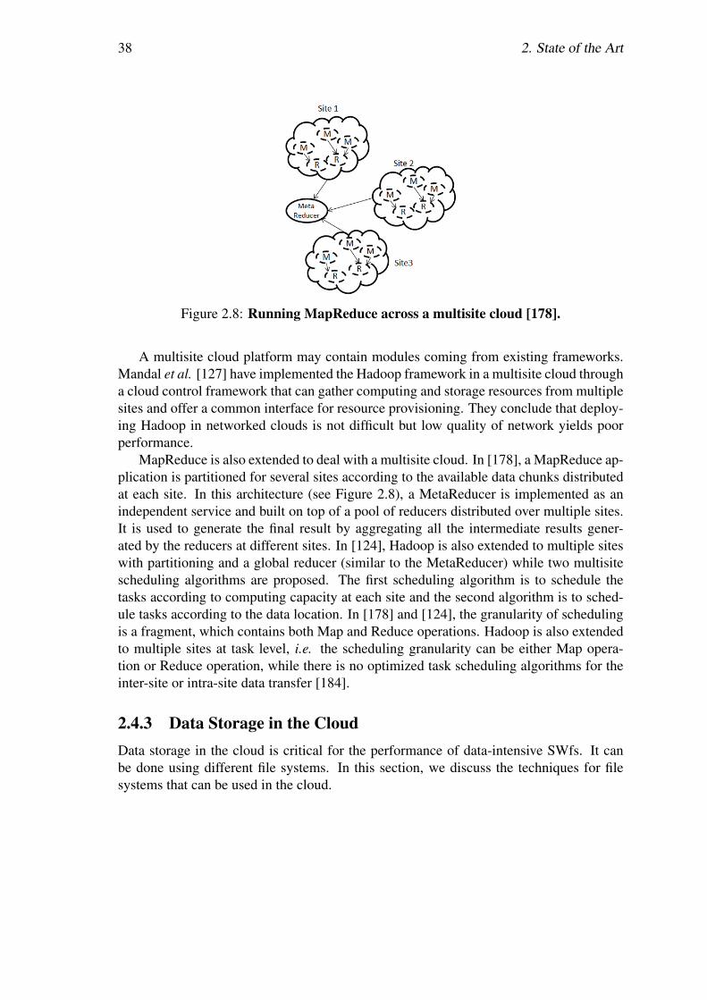
38 2. State of the Art
Figure 2.8: Running MapReduce across a multisite cloud [178].
A multisite cloud platform may contain modules coming from existing frameworks.Mandal et al. [127] have implemented the Hadoop framework in a multisite cloud througha cloud control framework that can gather computing and storage resources from multiplesites and offer a common interface for resource provisioning. They conclude that deploy-ing Hadoop in networked clouds is not difficult but low quality of network yields poorperformance.
MapReduce is also extended to deal with a multisite cloud. In [178], a MapReduce ap-plication is partitioned for several sites according to the available data chunks distributedat each site. In this architecture (see Figure 2.8), a MetaReducer is implemented as anindependent service and built on top of a pool of reducers distributed over multiple sites.It is used to generate the final result by aggregating all the intermediate results gener-ated by the reducers at different sites. In [124], Hadoop is also extended to multiple siteswith partitioning and a global reducer (similar to the MetaReducer) while two multisitescheduling algorithms are proposed. The first scheduling algorithm is to schedule thetasks according to computing capacity at each site and the second algorithm is to sched-ule tasks according to the data location. In [178] and [124], the granularity of schedulingis a fragment, which contains both Map and Reduce operations. Hadoop is also extendedto multiple sites at task level, i.e. the scheduling granularity can be either Map opera-tion or Reduce operation, while there is no optimized task scheduling algorithms for theinter-site or intra-site data transfer [184].
2.4.3 Data Storage in the CloudData storage in the cloud is critical for the performance of data-intensive SWfs. It canbe done using different file systems. In this section, we discuss the techniques for filesystems that can be used in the cloud.
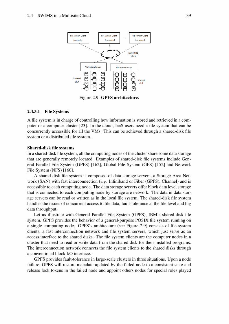
2.4 SWfMS in a Multisite Cloud 39
Figure 2.9: GPFS architecture.
2.4.3.1 File Systems
A file system is in charge of controlling how information is stored and retrieved in a com-puter or a computer cluster [23]. In the cloud, IaaS users need a file system that can beconcurrently accessible for all the VMs. This can be achieved through a shared-disk filesystem or a distributed file system.
Shared-disk file systemsIn a shared-disk file system, all the computing nodes of the cluster share some data storagethat are generally remotely located. Examples of shared-disk file systems include Gen-eral Parallel File System (GPFS) [162], Global File System (GFS) [152] and NetworkFile System (NFS) [160].
A shared-disk file system is composed of data storage servers, a Storage Area Net-work (SAN) with fast interconnection (e.g. Infiniband or Fiber (GPFS), Channel) and isaccessible to each computing node. The data storage servers offer block data level storagethat is connected to each computing node by storage are network. The data in data stor-age servers can be read or written as in the local file system. The shared-disk file systemhandles the issues of concurrent access to file data, fault-tolerance at the file level and bigdata throughput.
Let us illustrate with General Parallel File System (GPFS), IBM’s shared-disk filesystem. GPFS provides the behavior of a general-purpose POSIX file system running ona single computing node. GPFS’s architecture (see Figure 2.9) consists of file systemclients, a fast interconnection network and file system servers, which just serve as anaccess interface to the shared disks. The file system clients are the computer nodes in acluster that need to read or write data from the shared disk for their installed programs.The interconnection network connects the file system clients to the shared disks througha conventional block I/O interface.
GPFS provides fault-tolerance in large-scale clusters in three situations. Upon a nodefailure, GPFS will restore metadata updated by the failed node to a consistent state andrelease lock tokens in the failed node and appoint others nodes for special roles played
40 2. State of the Art
by the failed node. Upon a communication failure, the mechanism for one node lost ishandled as the node failures while a network equipment failure causes a network partition.In the case of partition, the nodes in the partition that has the highest number of nodeshave access to the shared disks. GPFS uses data replication across multiple disks to dealwith disk failures.
Cloud users can deploy a shared-disk file system by installing the correspondingframeworks (e.g. GPFS framework) in the VMs with the cloud storage resources suchas Microsoft Blob Storage and Amazon Elastic Block Store (EBS). Alternatively, cloudusers can mount Amazon Simple Storage Service (S3) into all the Linux-based VMs torealize the functionality that all the VMs can have access to the same storage resource, aswith a shared-disk file system.
Distributed file systemsA distributed file system stores data directly in the file system that is constructed by gath-ering storage space in each computing node in a shared-nothing architecture. The dis-tributed file system integrates solutions for load balancing among computing nodes, fault-tolerance and concurrent access. Files must be partitionned into chunks, e.g. through ahash function on records’ keys, and the chunks are distributed among computing nodes.Different from the shared-disk file system, computing nodes have to load the data chunksfrom the distributed file system to the local system before local processing.
Let us illustrate with Google File System (GFS) [80], which had a major impact oncloud data management. For instance, Hadoop Distributed File System (HDFS) is an opensource framework based on GFS. GFS is designed for a shared-nothing cluster made ofcommodity computers, and applications with frequent read operations while write oper-ations mainly consist of appending new data. GFS is composed of a single GFS masternode and multiple GFS chunk servers. The GFS master maintains all the file systemmetadata while GFS chunk servers store all the real data. The master can send instruc-tion information to the chunk servers while the chunk server can send chunk server statusinformation to the master. A GFS client can get the data location information from thefile namespace of the GFS master. Then it can write data to the GFS chunk servers at thisdata location or get the data chunks from a corresponding GFS chunk server according tothe data location information and required data size. This mechanism is shown in Figure2.10. GFS also provides snapshot support, garbage collection, fault-tolerance and diag-nosis. For high availability, GFS supports master replication and data chunk replication.
BlobSeer [135] is another distributed file system optimized for Binary Large OB-jects (BLOBs). The architecture of BlobSeer is shown in Figure 2.11. Data providersphysically store the data in the storage resources (data providers) while physical storageresources can be inserted or removed dynamically in the data providers. The providermanager tracks the information about the storage resources and schedules the placementof newly generated data. All the stored data has a version. Metadata providers storethe metadata for identifying data chunks that make up a snapshot version. The versionmanager assigns new snapshot version numbers to writers and appenders and reveals newsnapshots to readers. The write operation is performed in parallel on data chunks and

2.4 SWfMS in a Multisite Cloud 41
Figure 2.10: GFS architecture [80].
Figure 2.11: BlobSeer Architecture [135].
creates a new version of the data. Because of data versioning, read and write opera-tions can be asynchronous and thus improve the read and write throughput. The clientcan get the data location of the required files corresponding to the file name and therequired version when the required version is equal or inferior to the latest snapshot ver-sion. Then it can write data to the data providers or get the corresponding data chunksfrom the data providers by the data location and desired data size. BlobSeer also providesfault-tolerance through replication, consistency semantics and scalability based on sev-eral versioning mechanisms. Nicolae et al. [135] made a first performance comparison ofBlobster with HDFS, which shows important improvements in read and write thoughput,because of versioning.
Cloud users can deploy a distributed file system by installing corresponding frame-works (e.g. HDFS) of the aforementioned systems in available VMs to gather storageresources in each VM for executing applications in the Cloud.
2.4.4 Scientific Workflow Execution in the CloudThe cloud has some useful features to execute SWfs. In particular, the quality of serviceguaranteed by SLA can yield more stable performance. Juve et al. [103] compare the
42 2. State of the Art
performance of an astronomy application with the Pegasus SWfMS in the grid, the com-mercial cloud and the academic cloud. They conclude that the performance is the leaststable in grid and more stable in commercial cloud than academic cloud. We present theadaptations of SWfMSs for cloud environments, including SWf execution in a single sitecloud and that in multiple cloud sites.
2.4.4.1 Execution at a Single Cloud Site
In a single site cloud environment, SWfMSs can be directly installed in the VMs andexploit services deployed in the cloud [101, 191, 58]. Existing parallelization techniques,e.g. parallelism techniques (see Section 2.3.1), scheduling techniques (see Section 2.3.2),existing execution execution models in grid [58], can be used to execute a data-intensiveSWf in the environment. SWfMSs can exploit some middleware to create or remove VMsand enable the communication between VMs in order to execute data-intensive SWfs inthe cloud [90, 182, 17], such as Coasters [90] in Swift, Kepler EC2 actors [182] for Kepler,CloudMan [17] for Galaxy and RabbitMQ12 for Triana6 SWfMS. These tools can providecomputing or storage provisioning for SWf execution or communication between VMs.However, they cannot take advantage of the dynamic provisioning features of the cloud.
Some SWfMSs can take advantage of the scalability of cloud to provision VMs andstorage for SWf execution. For instance, Afgan et al. [17] propose CloudMan that permitsGalaxy to make use of Amazon EC2 and EBS for computing and storage provisioning forSWf execution. Some other SWfMSs are optimized for the cloud by supporting dynamicresource provisioning under budget and time limits, such as Pegasus [126, 133] withWrangler [102] (a dynamic provisioning system in the cloud) and Askalon [145, 144, 69]SWfMS. Since high parallelization degree can lead to less execution time, SWfMSs candynamically create new VMs in order to reduce execution time under monetary cost con-straint. But if the estimated monetary cost of SWf execution with current number of VMsexceeds the monetary cost constraint, SWfMSs can remove some VMs.
Chiron is adapted to the cloud through its extension, Scicumulus [51, 52]. The archi-tecture of Scicumulus contains three layers and four corresponding tiers: desktop layerfor client tier, distribution layer for distribution tier, execution layer for execution tier anddata tier. The desktop layer is to compose and execute SWfs. The distribution layer isresponsible for parallel execution of activities in the cloud. The execution layer man-ages activity execution in VM instances. Finally, the data tier manages the related dataduring SWf execution. Scicumulus exploits hybrid scheduling approaches with dynamiccomputing provisioning support. Furthermore, Scicumulus uses services such as SciDim[53] to determine an initial virtual cluster size through a multi-objective cost function andprovenance data under budget and time limits. Moreover, Scicumulus can be coupledwith SciMultaneous, which is used to manage fault tolerance in the cloud [45].
6Triana in cloud: http://www.trianacode.org/news.php
2.4 SWfMS in a Multisite Cloud 43
2.4.4.2 Execution in a Multisite Cloud
Clouds are independent of geographical distribution of physical resources by nature.However, it is possible to control the location of deployed services for better performancein some cloud environments, e.g. Microsoft Azure cloud [14] and Amazon cloud [12].In general, a user uses a single site, which is sufficient for most applications. However,there are important cases where SWfs will need to be deployed at several sites, e.g. be-cause the data accessed by the SWf is in different research groups’ databases in differentsites or because SWf execution needs more resources than those at a single site. Bigcloud providers such as Microsoft and Amazon typically have multiple geographicallydistributed data centers located at different sites. In some cases, a SWf must be executedat multiples sites. There are two approaches to do this. The first approach is to deploya SWfMS in a multisite cloud platform as discussed in Section 2.4.2. The second ap-proach is to make a SWfMS multisite-aware and capable to utilize computing and storageresources distributed at different sites. This is the approach we now focus on.
In a multisite cloud, we can execute a SWf with or without SWf partitioning. SWfexecution without partitioning is to schedule all the tasks into all the VMs in the multiplesites. This centralized method makes it hard to realize load balancing, incurs much over-head for each task and makes scheduling very complicated. With partitioning, a SWf isdivided in fragments (see Section 2.3.1) and each fragment is scheduled at a specific siteand its tasks scheduled within the VMs at this site. This method can reduce the overheadof task scheduling, which is done in parallel at multiple sites, and realize load balancingat two levels: inter-site and intra-site. Inter-site load balancing is realized by schedulingfragments, with a global scheduler, and intra-site load balancing is realized by local taskscheduling. This two-level approach makes the scheduling operation easier.
Swift and Pegasus achieve multisite execution by SWf partitioning. Swift performsSWf partitioning by generating corresponding abstract WEPs for each site [201]. Pegasusrealizes partitioning through several methods [38, 39]. As discussed in Section 2.2.2.3,Chen and Deelman [38] propose a SWf partitioning method under storage constraints ateach site. This SWf partitioning method is used in a multisite environment with dynamiccomputing provisioning as explained in [37]. Another method is balanced task clustering[39]. The SWf is partitioned into several fragments which have almost the same workload.This method can realize load balancing for homogeneous computing resources. Askaloncan execute SWf in a federated multisite cloud [145], i.e. a multisite cloud composed ofresources from different providers. Nevertheless, it schedules tasks in computing nodeswithout considering the organization of computing resources, i.e. which VMs are at thesame site, for optimization. This method just takes the VMs as the grid computing nodeswithout considering the features of multisite resources, e.g. the difference of data transferrate, resource sharing for intra-site and inter-site, etc.
44 2. State of the Art
2.4.5 Conclusion and RemarksThere are important cases where SWfs will need to be deployed at several data centersin the cloud, either from the same or different cloud providers, thus making multisitemanagement an important problem. Although some SWfMSs such as Swift and Pegasusprovide some functionality to execute SWfs in the multisite environment, this is gener-ally done by simply reusing the techniques from a grid environment or simple dynamicprovisioning and scheduling mechanisms, without exploiting new data storage and datatransfer capabilities provided by multisite clouds.
We believe that much more work is needed to improve the execution of data-intensiveSWfs in a multisite cloud. First, the co-scheduling of tasks and data should be exploited.Most SWfMSs make use of a shared file system to store data but do not care about wherethe data is stored for task scheduling. We believe that the co-scheduling of tasks and datacan be efficient at maximizing local data processing. Second, SWfMSs could optimizethe task scheduling while ensuring provenance support with the consideration of differentbandwidths among different sites. Third, the communication between two sites is gener-ally achieved by having two nodes, each at one of the two sites, communicating directly,which is not efficient in a multisite cloud. For instance, selecting several nodes at one siteto send or receive data to or from several nodes at another site could exploit parallel datatransfer and make it more efficient.
2.5 Overview of Existing SolutionsIn this section, we illustrate SWf parallel execution solutions in existing SWfMSs. Thissection starts by a short presentation of parallel processing frameworks such as MapRe-duce. Although they are not full-fledged SWfMS, they do share techniques in commonand are often used for complex scientific data analyses, or in conjunction with SWfMS todeal with big data [183]. Then, the section introduces eight widely used SWfMSs and ascience gateway platform. Finally, the section ends with concluding remarks.
2.5.1 Parallel Processing FrameworksParallel processing frameworks enable the programming and execution of big data analy-sis applications in massively parallel computing infrastructures.
MapReduce [55] is a popular parallel processing framework for shared-nothing clus-ters, i.e. highly-scalable clusters with no sharing of either disk or memory among com-puters. MapReduce was initially developed by Google as a proprietary product to processlarge amounts of unstructured or semi-structured data, such as web documents and logsof web page requests, on large shared-nothing clusters of commodity nodes and producevarious kinds of data such as inverted indices or URL access frequencies. Different im-plementations of MapReduce are now available such as Amazon MapReduce (as a cloudservice) or Hadoop [185].
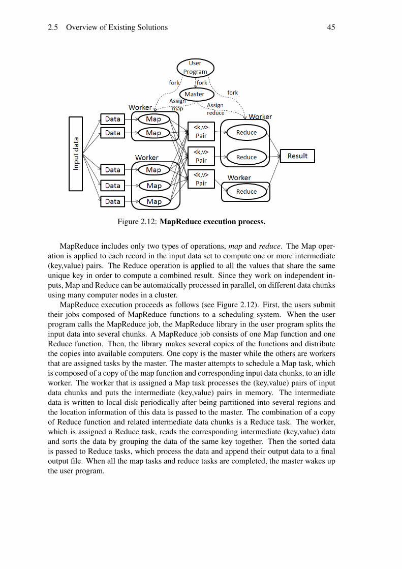
2.5 Overview of Existing Solutions 45
Figure 2.12: MapReduce execution process.
MapReduce includes only two types of operations, map and reduce. The Map oper-ation is applied to each record in the input data set to compute one or more intermediate(key,value) pairs. The Reduce operation is applied to all the values that share the sameunique key in order to compute a combined result. Since they work on independent in-puts, Map and Reduce can be automatically processed in parallel, on different data chunksusing many computer nodes in a cluster.
MapReduce execution proceeds as follows (see Figure 2.12). First, the users submittheir jobs composed of MapReduce functions to a scheduling system. When the userprogram calls the MapReduce job, the MapReduce library in the user program splits theinput data into several chunks. A MapReduce job consists of one Map function and oneReduce function. Then, the library makes several copies of the functions and distributethe copies into available computers. One copy is the master while the others are workersthat are assigned tasks by the master. The master attempts to schedule a Map task, whichis composed of a copy of the map function and corresponding input data chunks, to an idleworker. The worker that is assigned a Map task processes the (key,value) pairs of inputdata chunks and puts the intermediate (key,value) pairs in memory. The intermediatedata is written to local disk periodically after being partitioned into several regions andthe location information of this data is passed to the master. The combination of a copyof Reduce function and related intermediate data chunks is a Reduce task. The worker,which is assigned a Reduce task, reads the corresponding intermediate (key,value) dataand sorts the data by grouping the data of the same key together. Then the sorted datais passed to Reduce tasks, which process the data and append their output data to a finaloutput file. When all the map tasks and reduce tasks are completed, the master wakes upthe user program.
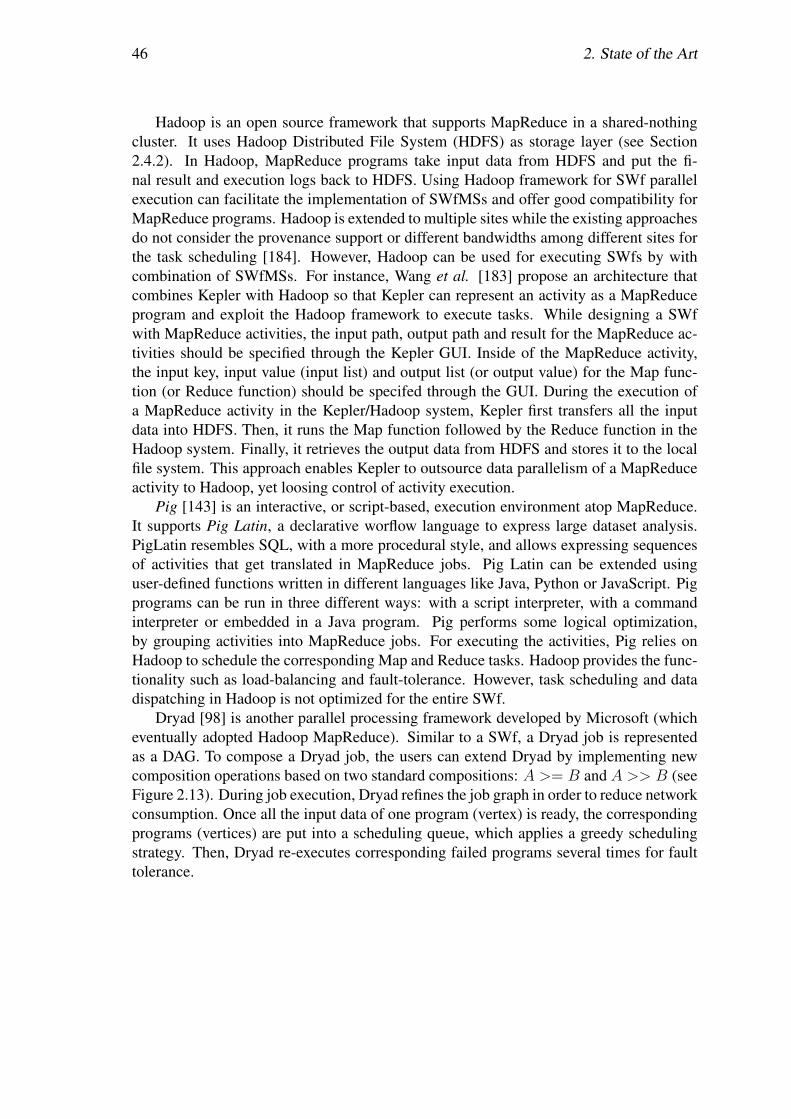
46 2. State of the Art
Hadoop is an open source framework that supports MapReduce in a shared-nothingcluster. It uses Hadoop Distributed File System (HDFS) as storage layer (see Section2.4.2). In Hadoop, MapReduce programs take input data from HDFS and put the fi-nal result and execution logs back to HDFS. Using Hadoop framework for SWf parallelexecution can facilitate the implementation of SWfMSs and offer good compatibility forMapReduce programs. Hadoop is extended to multiple sites while the existing approachesdo not consider the provenance support or different bandwidths among different sites forthe task scheduling [184]. However, Hadoop can be used for executing SWfs by withcombination of SWfMSs. For instance, Wang et al. [183] propose an architecture thatcombines Kepler with Hadoop so that Kepler can represent an activity as a MapReduceprogram and exploit the Hadoop framework to execute tasks. While designing a SWfwith MapReduce activities, the input path, output path and result for the MapReduce ac-tivities should be specified through the Kepler GUI. Inside of the MapReduce activity,the input key, input value (input list) and output list (or output value) for the Map func-tion (or Reduce function) should be specifed through the GUI. During the execution ofa MapReduce activity in the Kepler/Hadoop system, Kepler first transfers all the inputdata into HDFS. Then, it runs the Map function followed by the Reduce function in theHadoop system. Finally, it retrieves the output data from HDFS and stores it to the localfile system. This approach enables Kepler to outsource data parallelism of a MapReduceactivity to Hadoop, yet loosing control of activity execution.
Pig [143] is an interactive, or script-based, execution environment atop MapReduce.It supports Pig Latin, a declarative worflow language to express large dataset analysis.PigLatin resembles SQL, with a more procedural style, and allows expressing sequencesof activities that get translated in MapReduce jobs. Pig Latin can be extended usinguser-defined functions written in different languages like Java, Python or JavaScript. Pigprograms can be run in three different ways: with a script interpreter, with a commandinterpreter or embedded in a Java program. Pig performs some logical optimization,by grouping activities into MapReduce jobs. For executing the activities, Pig relies onHadoop to schedule the corresponding Map and Reduce tasks. Hadoop provides the func-tionality such as load-balancing and fault-tolerance. However, task scheduling and datadispatching in Hadoop is not optimized for the entire SWf.
Dryad [98] is another parallel processing framework developed by Microsoft (whicheventually adopted Hadoop MapReduce). Similar to a SWf, a Dryad job is representedas a DAG. To compose a Dryad job, the users can extend Dryad by implementing newcomposition operations based on two standard compositions: A >= B and A >> B (seeFigure 2.13). During job execution, Dryad refines the job graph in order to reduce networkconsumption. Once all the input data of one program (vertex) is ready, the correspondingprograms (vertices) are put into a scheduling queue, which applies a greedy schedulingstrategy. Then, Dryad re-executes corresponding failed programs several times for faulttolerance.
2.5 Overview of Existing Solutions 47
Figure 2.13: Dryad operations [98]. Circles represent programs and arrows representdata dependencies. Box (a) and box (b) illustrate program cloning with the ^ operator.We note each program P of type x as Px. The operation AS >= BS in (c) means thateach Pa has an input data flow to each Pb. The operation AS >> BS in (d) expressescomplete bipartite composition. Box (e) shows an operation by combining the data fromPb to Pc and Pd.
2.5.2 SWfMSMost SWfMSs implement the five layer architecture discussed in Section 2.2.2. Weselected eight typical SWfMSs and a gateway framework to illustrate their techniques:Pegasus, Swift, Kepler, Taverna, Chiron, Galaxy, Triana [173], Askalon [68] and WS-PGRADE/gUSE [105]. Pegasus and Swift have excellent support for scalability andhigh-performance of data-intensive SWfs, with reported results using more than a hundredthousand of cores and terabytes of data during SWf execution [61, 201]. Kepler, Taverna,Triana have a GUI for desktop computers. Chiron is widely used because of a powerfulalgebraic approach for SWf parallelization. Galaxy integrates a GUI that can be accessedthrough web browsers. Triana is able to use P2P services. Askalon implements both desk-top and web GUI and has been adapted to cloud environments. WS-PGRADE/gUSE is awidely used gateway framework, which enables SWf execution in Distributed ComputingInfrastructures (DCI) with a web interface for users.
Pegasus, Swift, Kepler, Taverna and WS-PGRADE/gUSE are widely used in astron-omy, biology, and so on while Galaxy can only execute bioinformatics SWfs. Pegasus,Swift and Chiron design and execute a SWf through a textual interface while Kepler, Tav-erna, Galaxy, Triana, Askalon and WS-PGRADE/gUSE integrate a GUI for SWf design.All of the eight SWfMSs and the gateway framework support SWf specification in a DAGstructure while Swift, Kepler, Chiron, Galaxy, Triana and Askalon also support SWfs ina DCG structure [195]. Users can share SWf information from Taverna, Galaxy, Askalonand WS-PGRADE/gUSE. All of them support independent parallelism. All of them sup-port dynamic scheduling and three of them (Pegasus, Kepler and WS-PGRADE/gUSE)support static scheduling. All the eight SWfMSs and the gateway framework supportSWf execution in both grid and cloud environments. A brief comparison of these eightSWfMSs and the gateway framework is given in Table 2.1.
48 2. State of the Art
2.5.2.1 Pegasus
Pegasus7 [61] is widely used in multiple disciplines such as astronomy, bioinformatics,climate modeling, earthquake science, genome analysis, etc. Pegasus has interesting fea-tures: portability on different infrastructures such as grid and cloud, optimized schedulingalgorithms; good scalability, support for provenance data that can be used for debugging,data transfer support for data-intensive SWfs, fault-tolerance support, detailed user guide[15] and available package in the Debian repository.
Pegasus consists of five components, i.e. mapper, local execution engine, job sched-uler, remote execution engine and monitoring component. The mapper generates an exe-cutable SWf and partitions SWf to fragments based on an abstract SWf provided by theusers. The local execution engine submits the fragments to execution engines accordingto dependencies. The job scheduler schedules the fragments to available remote execu-tion engines. The remote execution engine manages the execution of the tasks of thefragments. Finally, the monitoring component monitors the execution of the SWf.
The process of executing SWfs in Pegasus is shown in Figure 2.14. In the presenta-tion layer, Pegasus takes an abstract SWf represented as a DAX (DAG in an XML file).Pegasus provides programmatic APIs in Python, Java, and Perl for DAX generation[15].Pegasus exploits a lightweight web dashboard to monitor and the execution of SWfs fora user. In the user services layer, Pegasus supports SWf monitoring through Stampedemonitoring infrastructure [89, 159]. Pegasus also support provenance data gathering and
7Pegasus: http://pegasus.isi.edu/

2.5O
verviewofE
xistingSolutions
49
Table 2.1: Comparison of SWfMSs. A categorization of SWfMSs based on supported SWf structures, SWf information sharing,UI types, parallelism types and scheduling methods. “activity” means that this SWfMS supports both independent parallelism andpipeline parallelism. WPg represents WS-PGRADE/gUSE. WP indicates that the interface is a web-portal.
SWfMS structures SWf sharing UI type parallelism schedulingPegasus DAG not supported GUI & textual data & independent static & dynamic
Swift DCG not supported textual activity dynamicKepler DCG not supported GUI activity static & dynamicTaverna DAG supported GUI data & activity dynamicChiron DCG not supported textual data & activity & hybrid dynamicGalaxy DCG supported GUI (WP) independent dynamicTriana DCG not supported GUI data & activity dynamic
Askalon DCG supported GUI activity dynamic & hybridWPg DAG supported GUI (WP) data & independent & hybrid static & dynamic
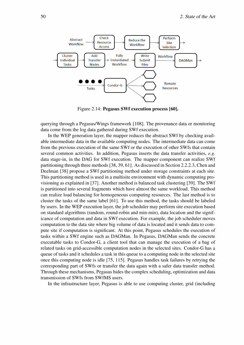
50 2. State of the Art
Figure 2.14: Pegasus SWf execution process [60].
querying through a Pegasus/Wings framework [108]. The provenance data or monitoringdata come from the log data gathered during SWf execution.
In the WEP generation layer, the mapper reduces the abstract SWf by checking avail-able intermediate data in the available computing nodes. The intermediate data can comefrom the previous execution of the same SWf or the execution of other SWfs that containseveral common activities. In addition, Pegasus inserts the data transfer activities, e.g.data stage-in, in the DAG for SWf execution. The mapper component can realize SWfpartitioning through three methods [38, 39, 61]. As discussed in Section 2.2.2.3, Chen andDeelman [38] propose a SWf partitioning method under storage constraints at each site.This partitioning method is used in a multisite environment with dynamic computing pro-visioning as explained in [37]. Another method is balanced task clustering [39]. The SWfis partitioned into several fragments which have almost the same workload. This methodcan realize load balancing for homogeneous computing resources. The last method is tocluster the tasks of the same label [61]. To use this method, the tasks should be labeledby users. In the WEP execution layer, the job scheduler may perform site execution basedon standard algorithms (random, round-robin and min-min), data location and the signif-icance of computation and data in SWf execution. For example, the job scheduler movescomputation to the data site where big volume of data is located and it sends data to com-pute site if computation is significant. At this point, Pegasus schedules the execution oftasks within a SWf engine such as DAGMan. In Pegasus, DAGMan sends the concreteexecutable tasks to Condor-G, a client tool that can manage the execution of a bag ofrelated tasks on grid-accessible computation nodes in the selected sites. Condor-G has aqueue of tasks and it schedules a task in this queue to a computing node in the selected siteonce this computing node is idle [75, 115]. Pegasus handles task failures by retrying thecorresponding part of SWfs or transfer the data again with a safer data transfer method.Through these mechanisms, Pegasus hides the complex scheduling, optimization and datatransmission of SWfs from SWfMS users.
In the infrastructure layer, Pegasus is able to use computing cluster, grid (including

2.5 Overview of Existing Solutions 51
desktop grids) and cloud to execute a SWf. It can exploit a shared file system, localstorage resources at each computing node or cloud storage, e.g. Amazon S3, for datastorage and it provides static computing and storage provisioning for SWf execution.Pegasus can be directly executed in a virtual cluster in cloud [101] while it can also usedynamic scheduling algorithms [126, 133] for budget constraint and time limit throughWrangler [102], a dynamic provisioning system in the cloud.
2.5.2.2 Swift
Similar to Pegasus, Swift [201] has been used in multiple disciplines such as biology,astronomy, economics, neuroscience, etc. Swift grew out of the GriPhyN Virtual DataSystem (VDS) whose objective is to express, execute, track the results of SWfs throughprogram optimization and scheduling, task management, and data management. Swift hasbeen revised and improved its (already) large-scale performance into the Turbine system[192].
Swift executes data-intensive SWfs through five functional phases: program speci-fication, scheduling, execution, provenance management and provisioning. In the pre-sentation layer, Swift takes a SWf specification that can be described in two languages:XDTM and SwfitScript. XDTM is an interface to map the logical structure of data tophysical resources. SwiftScript defines the sequential or parallel computational proce-dures that operate on the data defined by XDTM. In the user services layer, provenancedata is available for the users.
In the WEP generation layer, the SwiftScript is compiled to an abstract computationspecification. Swift performs partitioning by generating corresponding abstract WEPs foreach site [201]. In the WEP execution layer, the abstract WEPs are scheduled to execu-tion sites. The Karajan SWf execution engine is used by Swift to realize the functionssuch as data transfer, task submission, grid services access, task instantiation, and taskschedule. Swift runtime callouts provide the information for task and data scheduling andoffer status reporting, which shows the SPs. During SWf execution, provenance data isgathered by a launcher program (e.g. kickstart). Swift achieves fault tolerance by retryingthe failed tasks and provides a restart log when the failures are permanent.
In the infrastructure layer, the provisioning phase of Swift provides computing re-sources in a computer cluster, grid, and cloud through a dynamic resource provisionerfor each execution site. In the cloud, Swift takes advantage of Coasters [90] to managecommunication, task allocation and data stage for scientific SWf execution while it is notoptimized for dynamic provisioning of VMs and storage. Figure 2.15 depicts the Swiftsystem architecture.
2.5.2.3 Kepler
Kepler [21, 20] is a SWfMS built upon the Ptolemy II system from the Kepler8 project. Itallows to plug in different execution models into SWfs. Kepler is used in many projects of
8Kepler project: https://kepler-project.org/
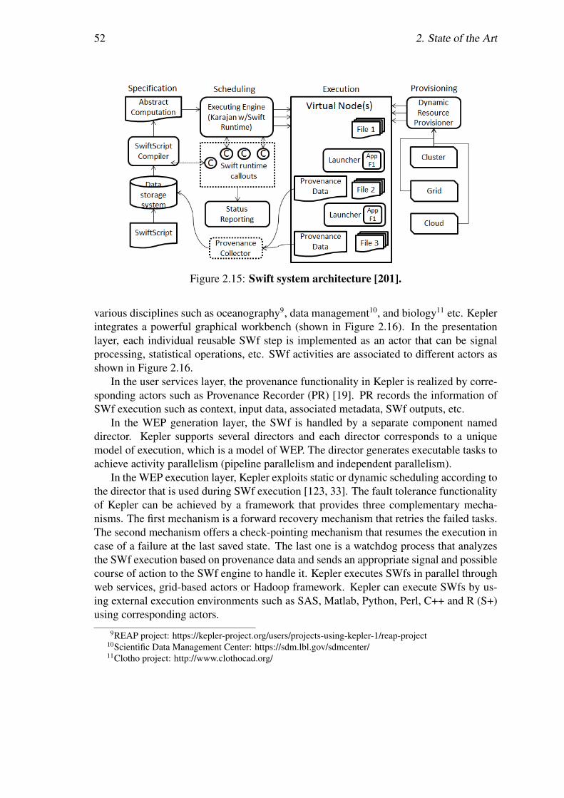
52 2. State of the Art
Figure 2.15: Swift system architecture [201].
various disciplines such as oceanography9, data management10, and biology11 etc. Keplerintegrates a powerful graphical workbench (shown in Figure 2.16). In the presentationlayer, each individual reusable SWf step is implemented as an actor that can be signalprocessing, statistical operations, etc. SWf activities are associated to different actors asshown in Figure 2.16.
In the user services layer, the provenance functionality in Kepler is realized by corre-sponding actors such as Provenance Recorder (PR) [19]. PR records the information ofSWf execution such as context, input data, associated metadata, SWf outputs, etc.
In the WEP generation layer, the SWf is handled by a separate component nameddirector. Kepler supports several directors and each director corresponds to a uniquemodel of execution, which is a model of WEP. The director generates executable tasks toachieve activity parallelism (pipeline parallelism and independent parallelism).
In the WEP execution layer, Kepler exploits static or dynamic scheduling according tothe director that is used during SWf execution [123, 33]. The fault tolerance functionalityof Kepler can be achieved by a framework that provides three complementary mecha-nisms. The first mechanism is a forward recovery mechanism that retries the failed tasks.The second mechanism offers a check-pointing mechanism that resumes the execution incase of a failure at the last saved state. The last one is a watchdog process that analyzesthe SWf execution based on provenance data and sends an appropriate signal and possiblecourse of action to the SWf engine to handle it. Kepler executes SWfs in parallel throughweb services, grid-based actors or Hadoop framework. Kepler can execute SWfs by us-ing external execution environments such as SAS, Matlab, Python, Perl, C++ and R (S+)using corresponding actors.
9REAP project: https://kepler-project.org/users/projects-using-kepler-1/reap-project10Scientific Data Management Center: https://sdm.lbl.gov/sdmcenter/11Clotho project: http://www.clothocad.org/
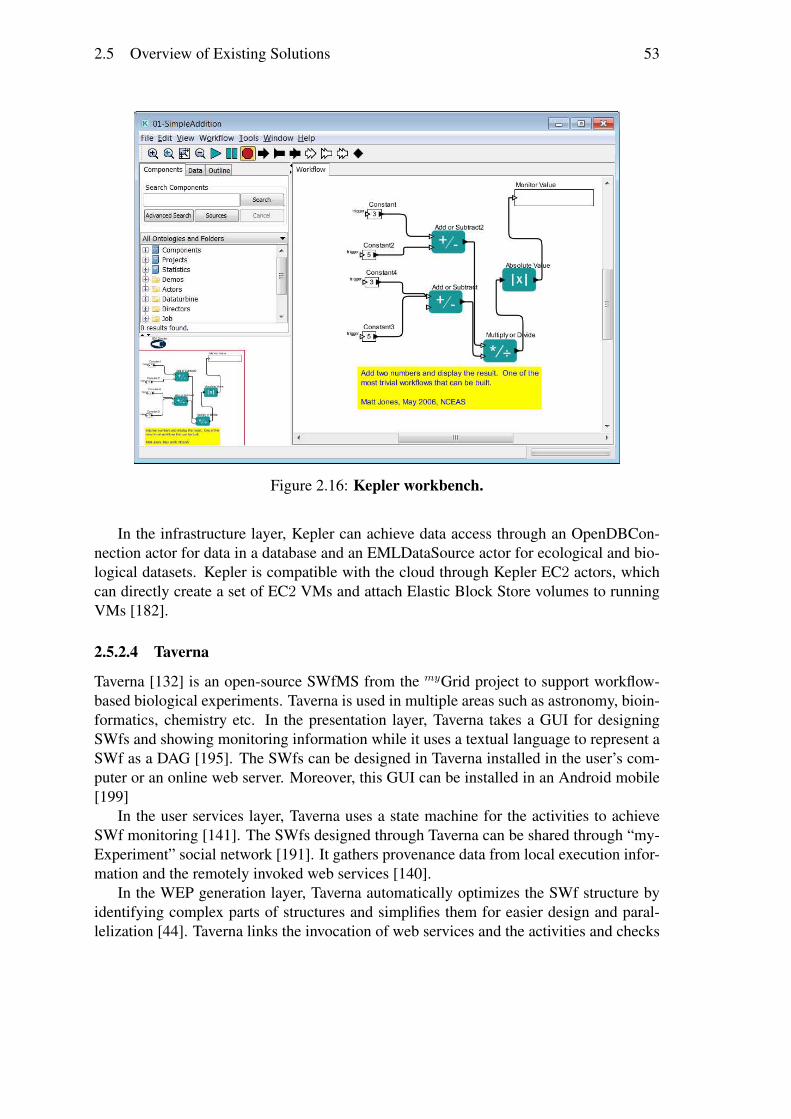
2.5 Overview of Existing Solutions 53
Figure 2.16: Kepler workbench.
In the infrastructure layer, Kepler can achieve data access through an OpenDBCon-nection actor for data in a database and an EMLDataSource actor for ecological and bio-logical datasets. Kepler is compatible with the cloud through Kepler EC2 actors, whichcan directly create a set of EC2 VMs and attach Elastic Block Store volumes to runningVMs [182].
2.5.2.4 Taverna
Taverna [132] is an open-source SWfMS from the myGrid project to support workflow-based biological experiments. Taverna is used in multiple areas such as astronomy, bioin-formatics, chemistry etc. In the presentation layer, Taverna takes a GUI for designingSWfs and showing monitoring information while it uses a textual language to represent aSWf as a DAG [195]. The SWfs can be designed in Taverna installed in the user’s com-puter or an online web server. Moreover, this GUI can be installed in an Android mobile[199]
In the user services layer, Taverna uses a state machine for the activities to achieveSWf monitoring [141]. The SWfs designed through Taverna can be shared through “my-Experiment” social network [191]. It gathers provenance data from local execution infor-mation and the remotely invoked web services [140].
In the WEP generation layer, Taverna automatically optimizes the SWf structure byidentifying complex parts of structures and simplifies them for easier design and paral-lelization [44]. Taverna links the invocation of web services and the activities and checks

54 2. State of the Art
the availability of the needed web services for generating a WEP. In the WEP executionlayer, Taverna relies on web and grid services for task execution.
In the infrastructure layer, Taverna is able to use the computing resources from grid orcloud. It also stores execution data in a database.
2.5.2.5 Chiron
Chiron exploits a database approach [146] to manage the parallel execution of data-intensive SWfs. In the presentation layer, it uses an algebraic data model to express alldata as relations and represent SWf activities as algebraic expressions in the presentationlayer. A relation contains sets of tuples composed of basic attributes such as integer, float,string, and file references, etc. An algebraic expression consists of algebraic activities,additional operands, operators, input relations and output relations. An algebraic activitycontains a program or an SQL expression, and input and output relation schemas. Anadditional operand is the side information for the algebraic expression, which can be re-lations or a set of grouping attributes. There are six operators: Map, SplitMap, Reduce,Filter, SRQuery and MRQuery (see Section 2.2.2.1 for the function of each operator). Inthe user services layer, Chiron supports SWf monitoring, steering and gathers provenancedata based on algebraic approach.
In the WEP generation layer, a SWf is wholly expressed in an XML file called con-ceptual model. Chiron supports all types of parallelism (data parallelism, independentparallelism, pipeline parallelism, hybrid parallelism) and optimizes SWf scheduling bydistinguishing between blocking activities, i.e. activities that require all their input datato proceed, and non blocking, i.e. that can be pipelined. Chiron generates concrete exe-cutable tasks for each activity and schedules the tasks of the same fragments to multiplecomputing nodes. Chiron uses two scheduling policies, called blocking and pipeline in[64]. Let A be a task that produces data consumed by a task B. With the blocking policy,B can start only after all the data produced by A are ready. Hence, there is no paral-lelism between A and B. With the pipeline policy, B can start as soon as some of its inputdata chunks are ready. Hence, there is pipeline parallelism. This pipeline parallelism isinspired by DBMS pipeline parallelism in [146]. Moreover, Chiron takes advantage ofalgebraic approach for SWf execution optimization to generate a WEP.
In the WEP execution layer, Chiron uses an execution module file to specify thescheduling method, database information and input data information. Chiron exploitsdynamic scheduling method for task execution. Chiron gathers execution data, light do-main data and provenance data into a database structured by following the PROV-Wf [46]provenance model. The execution of tasks in Chiron is based on MPJ [35], an MPI-likemessage passing system. In the infrastructure layer, Chiron exploits a shared-disk filesystem and database for data storage.
Chiron is adapted to the cloud through its extension, Scicumulus [51, 52], which sup-ports dynamic computing provisioning [50]. The architecture of Scicumulus containsthree layers and four corresponding tiers: desktop layer for client tier, distribution layerfor distribution tier, execution layer for execution tier and data tier. The desktop layer
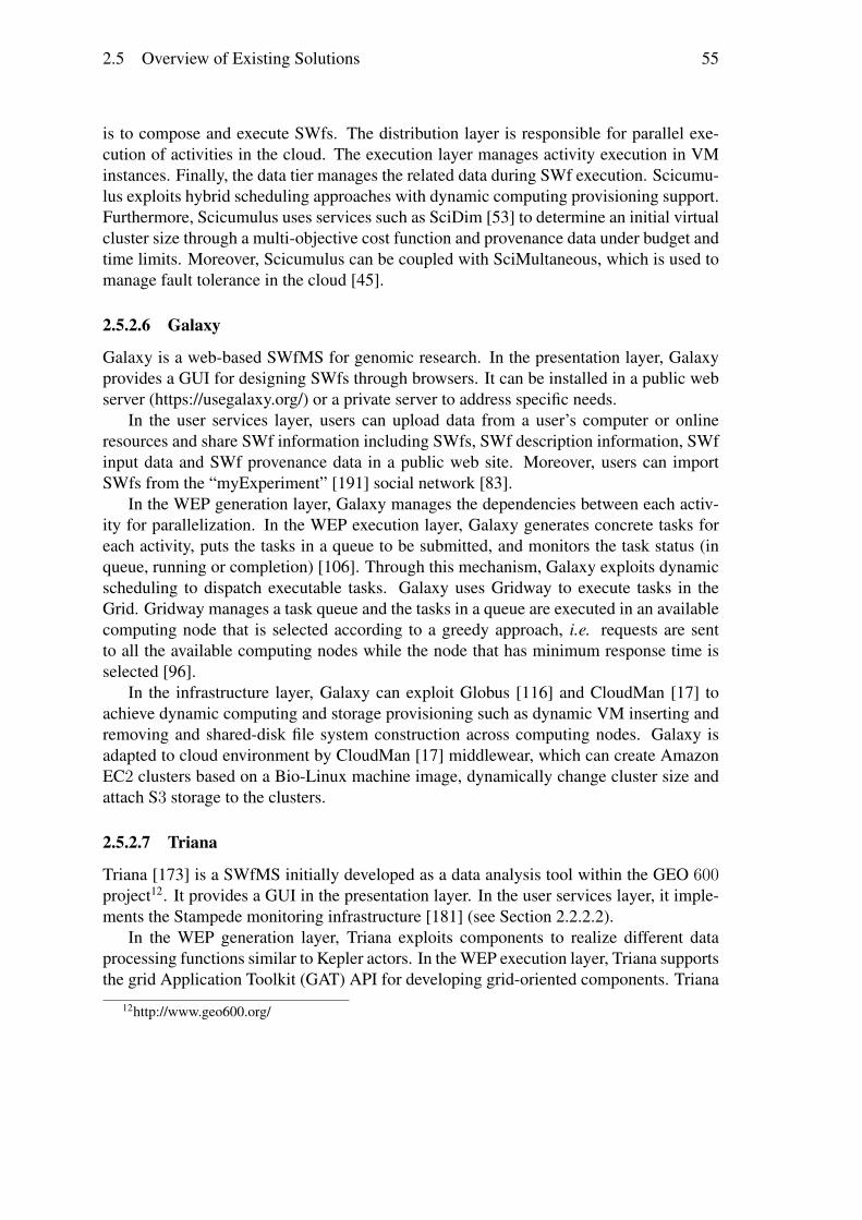
2.5 Overview of Existing Solutions 55
is to compose and execute SWfs. The distribution layer is responsible for parallel exe-cution of activities in the cloud. The execution layer manages activity execution in VMinstances. Finally, the data tier manages the related data during SWf execution. Scicumu-lus exploits hybrid scheduling approaches with dynamic computing provisioning support.Furthermore, Scicumulus uses services such as SciDim [53] to determine an initial virtualcluster size through a multi-objective cost function and provenance data under budget andtime limits. Moreover, Scicumulus can be coupled with SciMultaneous, which is used tomanage fault tolerance in the cloud [45].
2.5.2.6 Galaxy
Galaxy is a web-based SWfMS for genomic research. In the presentation layer, Galaxyprovides a GUI for designing SWfs through browsers. It can be installed in a public webserver (https://usegalaxy.org/) or a private server to address specific needs.
In the user services layer, users can upload data from a user’s computer or onlineresources and share SWf information including SWfs, SWf description information, SWfinput data and SWf provenance data in a public web site. Moreover, users can importSWfs from the “myExperiment” [191] social network [83].
In the WEP generation layer, Galaxy manages the dependencies between each activ-ity for parallelization. In the WEP execution layer, Galaxy generates concrete tasks foreach activity, puts the tasks in a queue to be submitted, and monitors the task status (inqueue, running or completion) [106]. Through this mechanism, Galaxy exploits dynamicscheduling to dispatch executable tasks. Galaxy uses Gridway to execute tasks in theGrid. Gridway manages a task queue and the tasks in a queue are executed in an availablecomputing node that is selected according to a greedy approach, i.e. requests are sentto all the available computing nodes while the node that has minimum response time isselected [96].
In the infrastructure layer, Galaxy can exploit Globus [116] and CloudMan [17] toachieve dynamic computing and storage provisioning such as dynamic VM inserting andremoving and shared-disk file system construction across computing nodes. Galaxy isadapted to cloud environment by CloudMan [17] middlewear, which can create AmazonEC2 clusters based on a Bio-Linux machine image, dynamically change cluster size andattach S3 storage to the clusters.
2.5.2.7 Triana
Triana [173] is a SWfMS initially developed as a data analysis tool within the GEO 600project12. It provides a GUI in the presentation layer. In the user services layer, it imple-ments the Stampede monitoring infrastructure [181] (see Section 2.2.2.2).
In the WEP generation layer, Triana exploits components to realize different dataprocessing functions similar to Kepler actors. In the WEP execution layer, Triana supportsthe grid Application Toolkit (GAT) API for developing grid-oriented components. Triana
12http://www.geo600.org/
56 2. State of the Art
also uses the Grid Application Prototype (GAP) as an interface to interact with service-oriented networks. The GAP contains three bindings, i.e. implemented GAP, such asP2PS and JXTA to use P2P network and Web services binding to invoke Web services.
In the infrastructure layer, Triana can employ computing resources in the grid or cloud.Triana uses RabbitMQ12 13, a message broker platform, to realize the communicationamong different VMs in order to run SWfs in the cloud environment.
2.5.2.8 Askalon
Askalon [68] is also a SWfMS initially designed for a grid environment. In the presenta-tion layer, it provides a GUI, through which a SWf can be modeled using Unified Model-ing Language. It also exploits an XML-based language to model workflows. In the userservices layer, it provides on-line SWf execution monitoring functionality through SWfexecution monitoring and dynamic workflow steering to deal with exceptions in dynamicand unpredictable execution environments [153].
In the WEP generation layer, Askalon optimizes the SWf representation with loops,i.e. within DCG structures, to a DAG SWf structure. In the WEP execution layer, Askalonexploits an execution engine to provide fault-tolerance at the levels of workflow, activityand control-flow. It can exploit static and hybrid scheduling, e.g. rescheduling because ofunpredictable changes in the execution environment.
In the infrastructure layer, Askalon uses a resource manager to discover and reserveavailable resources and to deploy executable tasks in the grid environment. Askalon isable to execute SWfs in cloud environment by dynamic creation of VMs with availablecloud images [145]. In the cloud environment, Askalon can estimate the cost of SWf exe-cution by simulation [144] and provide dynamic resource provisioning and task schedul-ing under budget constraint [69].
Moreover, Askalon can execute SWfs in a federated multisite cloud [145], i.e. a mul-tisite cloud composed of resources from different providers. Nevertheless, it schedulestasks in computing nodes without considering the organization of computing resources,i.e. which VMs are at the same site, for optimization. This method just takes the VMs asthe grid computing nodes without considering the features of multisite resources, e.g. thedifference of data transfer rate, resource sharing for intra-site and inter-site, etc.
2.5.2.9 WS-PGRADE/gUSE
WS-PGRADE/gUSE is a science gateway framework widely used in various disciplinessuch as biology [79], seismology [111], astronomy [163], and neuroscience [164]. It isan open source software [105] used for teaching [142], research [109] and commercialactivities [110].
The architecture of WS-PGRADE/gUSE framework is shown in Figure 2.17. WS-PGRADE portal is a web-portal interface to help the users designing SWfs. The grid andcloud User Support Environment (gUSE) is a middle layer for different user services. The
13Triana in cloud: http://www.trianacode.org/news.php

2.5 Overview of Existing Solutions 57
Figure 2.17: Architecture of WS-PGRADE/gUSE [87].
DCI bridge is a web service based application that provides access to divers infrastructuressuch as grid and cloud [105].
In the presentation layer, the WS-PGRADE portal [104] has a web browser based in-terface, which supports the definition of different kinds of SWfs, including meta-workflowsand parameter sweep workflows. The meta-workflows can contain embedded SWfs,which are supported by the SHIWA repository, as sub-workflows. In the user serviceslayer, WS-PGRADE supports SWf information sharing between the users of WS-PGRA-DE/gUSE through a build-in SWf repository, which enables publishing, searching anddownloading programs, SWf designs and templates [24]. A SWf template is an availableSWf pattern that can be changed to other SWfs by modifying corresponding parameters.In addition, it can exploit the SHIWA repository [151] to support SWf sharing betweenthe users of different SWfMSs. The monitoring functionality is supported by the gUSEservices. However, the framework lacks provenance support.
In the WEP generation layer, a SWf is represented in XML format. The frameworkmay use data and independent parallelism according to the structure of the SWf [24]. TheDCI bridge dynamically schedules the tasks through a submit queue. The task executionis handled by web services enabled by a web container, e.g. Tomcat or Glassfish.
Provisioning and data storage are provided by the DCI Bridge [113] and CloudBrokerframework. The DCI Bridge can dynamically create VMs through existing images andcloud configurations. The CloudBroker is able to exploit resources distributed in multipleclouds [71], including major cloud types , e.g. Amazon, OpenStack [99] and OpenNebula[131]. Moreover, it can take advantage of GPUs to execute the SWfs that invoke GPUprograms [24].
The SHIWA simulation platform enables reusing of SWfs in ten different SWfMS en-vironments [174]. First, the users can search for SWfs in the SHIWA repository, whereSWf developers can upload available programs or SWfs. Then, the SWfs can be down-loaded and adjusted to an Interoperable Workflow Intermediate Representation (IWIR)language to compose a meta-workflow [151]. Then, when the meta-workflow is submit-ted in the platform, each sub-workflow of the meta-workflow can be scheduled to theappropriate SWfMS execution environment.

58 2. State of the Art
2.5.3 Concluding RemarksWe observed that some SWfMSs take advantage of parallel processing frameworks suchas Hadoop as lower-level tools to parallelize SWf execution and schedule tasks. Thisis a straightforward approach to extend a SWfMS with parallel processing capabilities.However, it lacks the capability to perform parallelization according to the entire SWfstructure. Our comparative presentation of eight SWfMSs showed that most SWfMSs donot exploit hybrid parallelism (only Chiron does) and hybrid scheduling methods (onlyAskalon does), which may bring the highest degrees of parallelism and good load balanc-ing.
Although there has been much work on data-intensive SWf management, we believethere is a lot of room for improvement. First, input data staging needs more attention.Most SWfMSs just do this as a preprocessing step before actual SWf execution. Fordata-intensive SWfs, this step may take a very long time, for instance, to transfer severalgigabytes to a computing node. Integrating this step as part of the WEP can help optimizeit, based on the activities and their execution at computing nodes. Second, SWf parti-tioning strategies should pay attention to the computing capabilities of the resources anddata to be transferred across computing nodes, as this is a major performance and costfactor, and not focus only on one constraint, e.g. storage limitation. Third, although thereis already study on the VM provisioning techniques, it remains open problem to executeSWfs in a multisite cloud with the consideration of distributed data, features of the cloudsites. In addition, a cost model to estimate the execution of SWfs in a multisite cloud andcorresponding VM provisioning methods are also critical to the multisite SWf executionin the clouds. Fourth, the structure of SWfMSs is generally centralized (the new versionof Swift is not centralized). In this structure, a master node manages all the optimizationand scheduling processes. This master node becomes a single point of failure and perfor-mance bottleneck. Distributed and P2P techniques [147] could be applied to address thisproblem. Fourth, although most SWfMSs are capable to produce provenance data, theylack integrated UI with provenance data which is very useful for SWf steering.
2.6 ConclusionIn this chapter, we discussed the current state of the art of the SWfMSs, parallel executionof data-intensive SWfs in different infrastructures, especially in the cloud.
First, we introduced the definitions in SWf management, including SWfs and SWfMSs.In particular, we illustrated the representation of SWfs with real examples from astron-omy and biology. Then, we presented in more details a five-layer functional architectureof SWfMSs and the corresponding functions. Special attention has been paid to data-intensive SWfs by identifying their features and presenting the corresponding techniques.
Second, we presented the basic techniques for the parallel execution of SWfs inSWfMSs: parallelization and scheduling. We showed how different kinds of parallelism(coarse-grained parallelism, data parallelism, independent parallelism and pipeline paral-lelism) can be exploited for parallelizing SWfs. The scheduling methods to allocate tasks

2.6 Conclusion 59
to computing resources can be static or dynamic, with different trade-offs, or hybrid tocombine the advantages of static and dynamic scheduling methods. SWf scheduling mayinclude an optimization phase to minimize a multi-objective function, in a given context(cluster, grid, cloud). However, unlike in database query optimization, this schedulingoptimization phase is often not explicit and mixed with the scheduling method.
Third, we discussed cloud computing and the basic techniques for parallel executionof SWfs in the cloud, including single site cloud and multisite cloud. We discussed threecategories of cloud computing, multisite management in the cloud and data storage inthe cloud. The data storage techniques includes shared-disk file systems and distributedfile systems. Then, we analyzes the parallelization techniques of SWfs in both single sitecloud and multisite cloud.
Fourth, to illustrate the use of the techniques, we introduced the recent paralleliza-tion frameworks such as MapReduce and gave a comparative analysis of eight popularSWfMSs (Pegasus, Swift, Kepler, Taverna, Chiron, Galaxy, Triana and Askalon) and ascience gateway framework (WS-PGRADE/gUSE).
The current solutions for the parallel execution of SWfMSs are appropriate for staticcomputing and storage resources in a grid environment. They have been extended to dealwith more elastic resources in a cloud, but only with single site. Although some SWfMSssuch as Swift and Pegasus provide some functionality to execute SWfs in the multisiteenvironment, this is generally done by reusing techniques from grid computing or simpledynamic provisioning and scheduling mechanisms, without exploiting new data storageand data transfer capabilities provided by a multisite cloud. Our analysis of the currenttechniques of SWf parallelization and SWf execution has shown that there is a lot of roomfor improvement. And we proposed research directions addressed in this thesis (the firstfour points) and for future research, which we summarize as follows:
1. SWf partitioning: To partition a SWf into several parts based on resources in eachsite is also a difficult optimization problem in a multisite environment.
2. VM provisioning: In order to achieved multiple objectives, e.g. reducing executiontime and monetary cost, a cost model and corresponding VM provisioning methodis critical to SWf execution in a single cloud site or a multisite cloud. The costmodel could be optimized by considering the sequential workload and the cost toinitiate the cloud sites, i.e. creation and configuration of VMs.
3. Fragment scheduling: In order to execute a SWfs in a multisite cloud, it is alsoimportant to consider the distributed data at each site and different prices to useVMs at each site. A cost model and scheduling methods remain open problem forexecuting SWfs in a multisite with multiple objectives, e.g. reducing execution timeand monetary cost.
4. Task scheduling and data location: most SWfMSs do not take data location intoconsideration during task scheduling period. For data-intensive SWfs, a uniformscheduling method is needed to handle task and data scheduling at the same time.

60 2. State of the Art
Furthermore, SWfMSs should also consider provenance support for SWf executionwith different bandwidths among different sites.
5. Multisite Data transfer: the current data transfer methods between two sites are re-alized by two nodes, each of which located at a site. We believe that using multiplenodes at each site can achieve bigger bandwidths. However, the problem of map-ping heterogeneous computing nodes at a site to the computing nodes at anothersite requires better algorithms.
Chapter 3
Scientific Workflow Partitioning in aMultisite Cloud
As the scale of the data increases, SWfMSs need to support SWf execution in High Per-formance Computing (HPC) environments. Because of various benefits, cloud emerges asan appropriate infrastructure for SWf execution. However, it is difficult to execute someSWfs at a cloud site because of geographical distribution of scientists, data and computingresources. Therefore, a SWf often needs to be partitioned and executed in a multisite en-vironment. This chapter proposes a non-intrusive approach to execute SWfs in a multisitecloud with three SWf partitioning techniques. This chapter is based on [122].
Section 3.3 introduces our system model based on an adaptation of Chiron for multi-site cloud. Then, Section 3.4 presents the Buzz SWf we use for experimentation. Section3.5 details our three SWf partitioning techniques and Section 3.6 presents our experi-mental validation in Microsoft Azure. The experimental validation used an adaptation ofChiron SWfMS for Microsoft Azure multisite cloud. The experiment results reveal theefficiency of our partitioning techniques, and their superiority in different environments.
3.1 Overview of the Proposal and MotivationsScientific experiments generally contain multiple computational activities to process ex-perimental data and these activities are related by data or control dependencies. SWfsenable scientists to model these data processing activities together to be automatically ex-ecuted. In a SWf, one activity may consist of several executable tasks for different partsof experimental data during SWf execution. SWfs exploit SWfMSs to manage SWf rep-resentation, execution and data sets in various computing environments. SWfMSs mayexploit High Performance Computing (HPC) to execute SWfs within reasonable time.The HPC environment may be provided by a cluster, grid or cloud. Cloud computing,which promises virtually infinite resources, scalable services, stable service quality andflexible payment policies, has recently become a viable solution for SWf execution.
In general, one cloud site is sufficient for executing one user application. However,
61
62 3. Scientific Workflow Partitioning in a Multisite Cloud
in the case of SWfs, some important restrictions may force their execution in a multisitecloud, i.e. a cloud with multiple distributed data centers, each being explicitly accessibleto cloud users. For instance, some activities need to be executed at a cloud site trusted bythe scientists for SWf monitoring without malicious attack, i.e. scientist security restric-tion; some activities need to be moved to another cloud site because of stored big inputdata at that site and the cost of transferring this big data to another site is very high, i.e.data transfer restriction; some activities have to be executed at a site where more comput-ing resources are available, i.e. computing capacity restriction; some other activities mayinvoke special programs (instruction data), which are located at a specific cloud site andcannot be moved to another site because of proprietary reasons, i.e. proprietary restric-tion. The configuration data, which includes SWf representation files or SWf parameters,can be located at one site or distributed at different sites. In this situation, multisite cloudis appealing for data-intensive SWfs.
For a given application, a multisite cloud configuration, which is the configuration ofVirtual Machines (VMs) at each site, can be homogeneous, with homogeneous computingcapacity at each site, e.g. 8 VMs at sites 1 and 2, or heterogeneous, e.g. 8 VMs at site 1 and2 VMs at site 2. The homogeneous configuration is obviously easier to deal with in termsof SWf partitioning and execution. However, even the homogeneous configuration makesit difficult to reproduce experiments as the allocation of VMs to real resources is typicallycontrolled at runtime by the cloud provider. For instance, at time t1, one VM may beallocated to a processor that is already very busy (e.g. running 16 other VMs) while attime t2, the same VM may be allocated to an underloaded processor (e.g. running 2 otherVMs).
In order to execute SWfs in a multisite cloud environment, a SWfMS can generatea Workflow Execution Plan (WEP) for SWf execution. Similar to the concept of QueryExecution Plan (QEP) in distributed database systems [146], the WEP is a program thatcaptures optimization decisions and execution directives, typically the result of compilingand optimizing a SWf. Since the multiple sites are interconnected but share nothing, theWEP includes a SWf partitioning result, which is the decision of partitioning a SWf intoSWf fragments for independent execution. A SWf fragment (or fragment for short) can bedefined as a subset of activities and data dependencies of the original SWf (see [138] fora formal definition). In order to execute a fragment within reasonable time at one site, theWEP generally contains a SWf parallelization plan, which parallelizes SWf execution.
We formulate the problems addressed in this chapter as follows. A SWf W = {V ,E}consists of a set of activities V and a set of dependencies E. A multisite cloud MS = {S1,S2, ..., Sn} is composed of multiple cloud sites, each of which has multiple computingnodes and stores its own data (input data, instruction data or configuration data ofW ). TheSWf execution time is the entire time to execute a SWf at a given execution environment.Given a SWf W and a multisite cloud MS, the multisite cloud execution problem is howto execute W in MS in a way that reduces execution time while respecting restrictions.
We propose a non-intrusive approach to execute a SWf in a multisite cloud. We pro-pose three partitioning techniques with the consideration of restrictions. We validate ourapproach with a data-intensive SWf using Chiron [139] SWfMS in Microsoft Azure [5]

3.2 Related Work 63
cloud. The experiment results reveal that our approach can reduce execution time. Sincethe occupied computing resources do not change, the reduction of execution time maylead to less lease time, which corresponds to less monetary cost.
3.2 Related WorkSWf partitioning and execution in a multisite cloud remains a challenge and little workhas been done. Deng et al. [62] adopt a clustering method based on data-data, data-activity and activity-activity dependencies. This method is adapted for SWf structures,but it may have big amount of data to be transferred among fragments. Chen et al. [37]present SWf partitioning based on storage constraints. Since a cloud environment can of-fer big storage capacity and the VMs can be mounted additional storage resources beforeor during SWf exeuciton, the storage capacity limitation is not general in a cloud envi-ronment. In addition, this method do not take data transfer cost and different computingcapacity at each site into consideration. Tanaka and Tatebe [171] use a Multi-ConstraintGraph Partitioning (MCGP) algorithm [107] to partition a SWf. This approach partitionsa SWf by minimizing the removed dependency and balancing the activities in each frag-ment. However, this approach is appropriate only for homogeneous execution sites. Inthis chapter, we propose several partitioning techniques to address data transfer restrictionand computing capacity restriction in the multisite cloud. Because of SWf partitioning,distributed provenance data is supported in the multisite cloud. In addition, data compres-sion and file archiving is proposed to accelerate the data transfer between different cloudsites.
3.3 System ModelIn this section, we present our system model based on Chiron SWfMS, its adaptation formultisite cloud and a SWf partitioner.
Chiron implements an algebraic approach for data-intensive SWfs proposed by Oga-sawara et al. [139], to perform SWf parallelization and scheduling. This approach asso-ciates each activity with an operator, which has a semantic meaning for parallel execution.Since it models SWf data as relations similar to relational database management systems,this approach can optimize the entire SWf parallel execution based on well-founded rela-tional algebra query optimization models [138].
The algebraic approach also allows online provenance data to be managed (and storedin a database by Chiron) for SWf activity monitoring [46]. Provenance data is the meta-data that captures the derivation history of a dataset, including the original data sources,intermediate datasets, and the SWf computational steps that were applied to produce thisdataset [46].
Chiron was initially developed for a one site execution environment as shown in Fig.3.1-A. In a one site environment, a database is installed in a master node and all thecomputing nodes share storage resources through Network File System. Chiron achieves
64 3. Scientific Workflow Partitioning in a Multisite Cloud
activity parallelism, data parallelism and dynamic scheduling for SWf parallelization asexplained in Section 3.2. Chiron was modified to gather necessary produced data at theend of SWf execution at one site.
In a multisite cloud environment (see Fig. 3.1-B), all the sites have the same con-figuration as one site environment, i.e. a database installed in a master node and sharedstorage resources, while each site can have different numbers of slave computing nodes.We developped a SWf partitioner to automatically partition a processed SWf representa-tion file into SWf fragment representation files when the first activity in each fragmentis given. All the activities in a fragment are placed together in the processed SWf rep-resentation file. The SWf partitioner removes the dependencies in the original SWf andgenerates corresponding configuration files for each fragment. The execution of the gen-erated fragments should respect the dependencies removed from the original SWf. Letus suppose that, in a SWf, activity A2 consumes the output data produced by activity A1.If these two activities are allocated to different fragments, their data dependencies willbe removed from the explicit data dependencies. In this case, the fragment that containsactivity A2 should be executed after the execution of the fragment that contains activityA1.
In order to reduce data transfer volume between different sites, we can use data com-pression and file archiving techniques. Data compression can just reduce the volume oftransferred data to reduce transmission time. Through file archiving, we can also transferthe data at a relatively high speed to reduce transmission time. When transferring one filebetween two sites and the default transfer speed is less than the average transfer speedbetween two sites, the file transfer is accelerated (accelerating phase) at the beginningand decreased (decreasing phase) at the end. The data transfer rate remains high in themiddle (high speed transfer phase). If we transfer several small files, there will be manyaccelerating and decreasing phases. But if we transfer a big file of the same data volume,there will be an accelerating phase and a decreasing phase while the high speed transferphase will be longer. Therefore, the transmission speed of a big file is higher than that ofseveral small files of the same data volume. In the remainder of the chapter, we note datarefining as the combination of file archiving and data compression.
3.4 Use Case: Buzz WorkflowThis section presents Buzz SWf [64], a data-intensive SWf, as a use case to illustrateour partitioning techniques. Buzz SWf is modeled and executed using Chiron. BuzzSWf searches for trends and measures correlations in published papers from scientificpublications. This SWf uses data collected from bibliography databases such as the DBLPComputer Science Bibliography (DBLP) [4] or the U.S. National Institutes of Health’sNational Library of Medicine (PubMed). We used a DBLP 2013 XML file of 1, 29GB asinput for Buzz SWf in our experiments.
Buzz SWf has thirteen activities (Fig. 3.2(a)). Each activity has a specific operator ac-cording to the algebraic approach. Boxes in the figure represent activities together with the
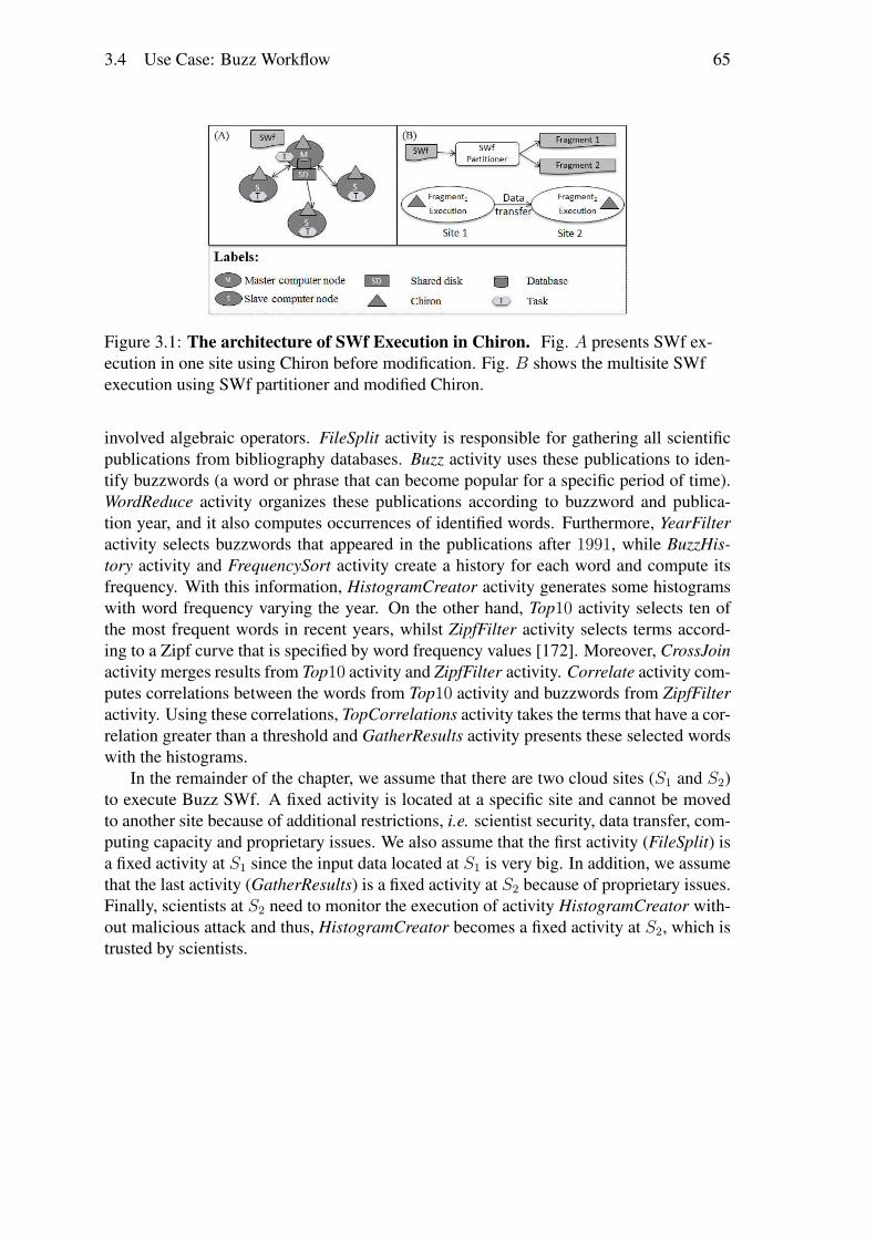
3.4 Use Case: Buzz Workflow 65
Figure 3.1: The architecture of SWf Execution in Chiron. Fig. A presents SWf ex-ecution in one site using Chiron before modification. Fig. B shows the multisite SWfexecution using SWf partitioner and modified Chiron.
involved algebraic operators. FileSplit activity is responsible for gathering all scientificpublications from bibliography databases. Buzz activity uses these publications to iden-tify buzzwords (a word or phrase that can become popular for a specific period of time).WordReduce activity organizes these publications according to buzzword and publica-tion year, and it also computes occurrences of identified words. Furthermore, YearFilteractivity selects buzzwords that appeared in the publications after 1991, while BuzzHis-tory activity and FrequencySort activity create a history for each word and compute itsfrequency. With this information, HistogramCreator activity generates some histogramswith word frequency varying the year. On the other hand, Top10 activity selects ten ofthe most frequent words in recent years, whilst ZipfFilter activity selects terms accord-ing to a Zipf curve that is specified by word frequency values [172]. Moreover, CrossJoinactivity merges results from Top10 activity and ZipfFilter activity. Correlate activity com-putes correlations between the words from Top10 activity and buzzwords from ZipfFilteractivity. Using these correlations, TopCorrelations activity takes the terms that have a cor-relation greater than a threshold and GatherResults activity presents these selected wordswith the histograms.
In the remainder of the chapter, we assume that there are two cloud sites (S1 and S2)to execute Buzz SWf. A fixed activity is located at a specific site and cannot be movedto another site because of additional restrictions, i.e. scientist security, data transfer, com-puting capacity and proprietary issues. We also assume that the first activity (FileSplit) isa fixed activity at S1 since the input data located at S1 is very big. In addition, we assumethat the last activity (GatherResults) is a fixed activity at S2 because of proprietary issues.Finally, scientists at S2 need to monitor the execution of activity HistogramCreator with-out malicious attack and thus, HistogramCreator becomes a fixed activity at S2, which istrusted by scientists.
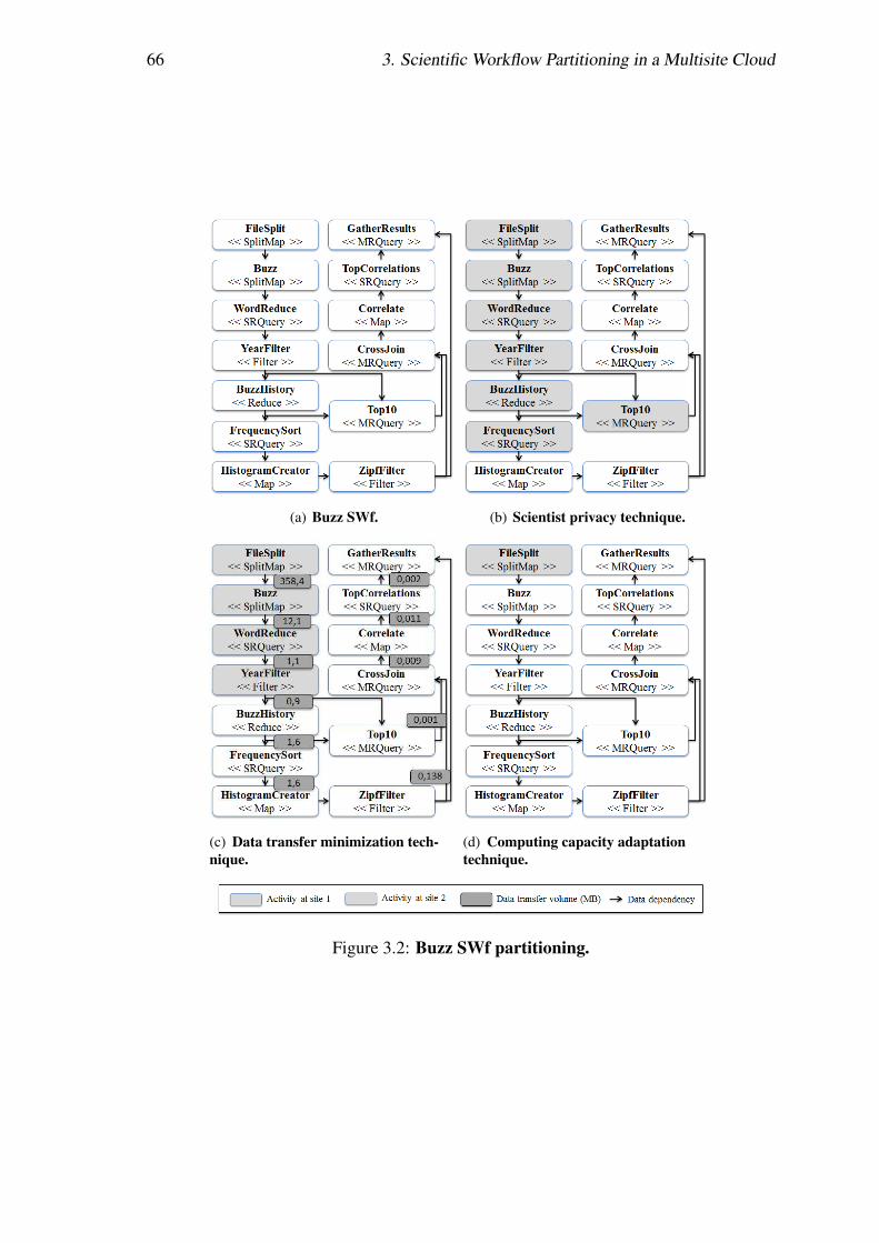
66 3. Scientific Workflow Partitioning in a Multisite Cloud
(a) Buzz SWf. (b) Scientist privacy technique.
(c) Data transfer minimization tech-nique.
(d) Computing capacity adaptationtechnique.
Figure 3.2: Buzz SWf partitioning.
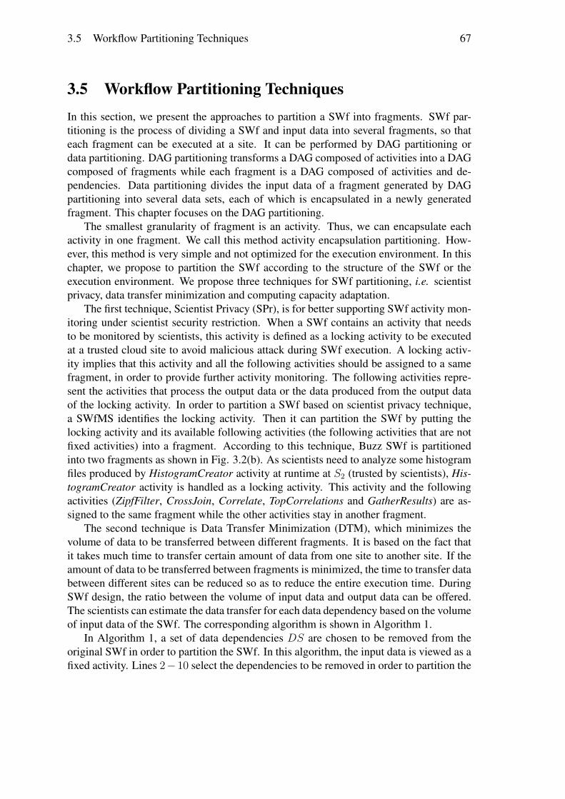
3.5 Workflow Partitioning Techniques 67
3.5 Workflow Partitioning TechniquesIn this section, we present the approaches to partition a SWf into fragments. SWf par-titioning is the process of dividing a SWf and input data into several fragments, so thateach fragment can be executed at a site. It can be performed by DAG partitioning ordata partitioning. DAG partitioning transforms a DAG composed of activities into a DAGcomposed of fragments while each fragment is a DAG composed of activities and de-pendencies. Data partitioning divides the input data of a fragment generated by DAGpartitioning into several data sets, each of which is encapsulated in a newly generatedfragment. This chapter focuses on the DAG partitioning.
The smallest granularity of fragment is an activity. Thus, we can encapsulate eachactivity in one fragment. We call this method activity encapsulation partitioning. How-ever, this method is very simple and not optimized for the execution environment. In thischapter, we propose to partition the SWf according to the structure of the SWf or theexecution environment. We propose three techniques for SWf partitioning, i.e. scientistprivacy, data transfer minimization and computing capacity adaptation.
The first technique, Scientist Privacy (SPr), is for better supporting SWf activity mon-itoring under scientist security restriction. When a SWf contains an activity that needsto be monitored by scientists, this activity is defined as a locking activity to be executedat a trusted cloud site to avoid malicious attack during SWf execution. A locking activ-ity implies that this activity and all the following activities should be assigned to a samefragment, in order to provide further activity monitoring. The following activities repre-sent the activities that process the output data or the data produced from the output dataof the locking activity. In order to partition a SWf based on scientist privacy technique,a SWfMS identifies the locking activity. Then it can partition the SWf by putting thelocking activity and its available following activities (the following activities that are notfixed activities) into a fragment. According to this technique, Buzz SWf is partitionedinto two fragments as shown in Fig. 3.2(b). As scientists need to analyze some histogramfiles produced by HistogramCreator activity at runtime at S2 (trusted by scientists), His-togramCreator activity is handled as a locking activity. This activity and the followingactivities (ZipfFilter, CrossJoin, Correlate, TopCorrelations and GatherResults) are as-signed to the same fragment while the other activities stay in another fragment.
The second technique is Data Transfer Minimization (DTM), which minimizes thevolume of data to be transferred between different fragments. It is based on the fact thatit takes much time to transfer certain amount of data from one site to another site. If theamount of data to be transferred between fragments is minimized, the time to transfer databetween different sites can be reduced so as to reduce the entire execution time. DuringSWf design, the ratio between the volume of input data and output data can be offered.The scientists can estimate the data transfer for each data dependency based on the volumeof input data of the SWf. The corresponding algorithm is shown in Algorithm 1.
In Algorithm 1, a set of data dependencies DS are chosen to be removed from theoriginal SWf in order to partition the SWf. In this algorithm, the input data is viewed as afixed activity. Lines 2− 10 select the dependencies to be removed in order to partition the
68 3. Scientific Workflow Partitioning in a Multisite Cloud
Input: SWf : a SWf; S: a set of sitesOutput: DS: a set of dependencies to cut in order to partition the SWfbegin
1: DS ← ∅2: for each s ∈ S do3: A← fixedActvities(SWf, s)4: A′ ← fixedOutsideUnprocessedActivities(SWf, s)5: for each a ∈ A do6: for each a′ ∈ A′ do7: paths← findPaths(a, a′)8: for each path ∈ paths do9: ds← minData(path)
10: DS ← DS⋃ds
11: end for12: end for13: end for14: end for15: DS ← sort(DS)16: for each ds ∈ DS do17: if SWf can be partitioned by DS without ds) then18: DS ← DS − ds19: end if20: end forend
algorithm 1: Data transfer minimization SWf partitioning
activities of the SWf at each site. Line 4 selects the fixed activities that are outside of Sites and that the corresponding sites are not processed. If one site is processed in the loopof Lines 5 − 11, it is marked as processed. For the two functions fixedActivities andfixedOutsideUnprocessedActivities, each activity is checked to know if the activityis to be selected. Lines 7 − 10 choose the dependencies to be removed so that the fixedactivities at Site s are not connected with the fixed activities at other sites. Line 7 findsall the paths that connect two activities fixed at different sites. A path has a set of datadependencies that can connect two activities without consideration of direction. In orderto find all the paths, a depth-first search algorithm can be used. For each path (Line 8), thedata dependency that has the least amount of data to be transferred is selected (Line 9) toDS (Line 10). At the same time, the input activity and output activity of the selected datadependency are marked. Line 11 sorts the data dependencies according to the amount ofdata to be transferred in descending order. If two or more data dependencies have the sameamount of data, they are sorted according to the amount of output data of the followingactivity of each data dependency in descending order. This order allows the activities thathave bigger data dependencies with their following activities to be connected with their
3.6 Validation 69
following activities, after the removing of dependencies (Lines 12−14), in order to reducethe amount of data to be transferred among different fragments. Lines 12−14 remove datadependencies from DS while ensuring that the SWf can always be partitioned with DS.Checking if SWf can be partitioned by a set of dependencies can be realized by checkingif the corresponding input and output activities of ds are connected with a depth-firstsearch algorithm (Line 13).
With this algorithm, Buzz SWf is partitioned as shown in Fig. 3.2(c). The dark grayboxes represent the data transfer volume for the corresponding dependencies. The datadependencies of each possible route between FileSplit and HistogramCreator is analyzed.The dependencies (YearFilter to BuzzHistory and YearFilter to Top10) are put in DS tobe removed. Finally, Buzz SWf is partitioned by removing the selected dependencies(YearFilter to BuzzHistory and YearFilter to Top10).
The third technique is Computing Capacity Adaptation (CCA), which adapts SWfspartitioning to the computing capacity at different cloud sites. This technique is for theheterogeneous multisite cloud configurations, which may be incurred by the differentconfigurations of different groups of scientists. If a SWf is partitioned into two fragmentsthat are sequentially executed, i.e. one fragment begins execution after the execution ofanother one, a SWfMS can put all the possible activities to one fragment while leavingfixed activities in another fragment. As an example, Buzz SWf is partitioned into twofragments (WF1 and WF2) as shown in Fig. 3.2(d) . Since the input data of activityFileSplit is relatively big and located at a specific site, we keep this activity in the grayfragment. Then, the white fragments can be scheduled to a cloud site that has morecomputing capacity.
3.6 ValidationIn this section, we present experiments to validate our approach, by executing Buzz SWfusing our partitioning techniques in Microsoft Azure cloud. The VMs are distributedat two cloud sites: Western Europe (Amsterdam, Netherlands) and Eastern US (NorthVirginia). In the first experiment, we use a homogeneous configuration by creating twoA4 VMs at both of Western Europe site and Eastern US site. In the second experiment,we use a heterogeneous configuration by creating two A4 VMs at the Western Europe siteand eight A4 VMs at the Eastern US site. Each A4 VM has 8 CPU cores, 14 GB of RAMmemory, 127 GB of instance storage and a network of 800 Mbps [11, 10].
We executed Buzz SWf with Chiron and the SWf partitioner. We used Linux tarcommand and Linux scp command for data refining and data transfer. We launched thefragment execution by hand at each cloud site, which resembles to the cooperation be-tween two scientist group. In our execution, Chiron exploits data parallelism and thedynamic scheduling method for SWf parallel execution within one site. Table 3.1 showsthe experimental results. Elapsed time 1 represents the execution time without consid-ering data transfer time. Elapsed time 2 shows the execution time plus the data transfertime. Elapsed time 3 is the execution time plus data transfer time with data refining. Data

70 3. Scientific Workflow Partitioning in a Multisite Cloud
Table 3.1: Experimental Results.
Approach Execution Transmission Execution Transmission Execution(Time in minutes) time 1 time 1 time 2 time 2 time 3
1st experiment 2*A4 VM (EU) + 2*A4 VM (US)SPr technique 199 38 237 0 199
DTM technique 186 0 186 0 186CCA technique 209 35 245 0.5 2091st experiment 2*A4 VM (EU) + 8*A4 VM (US)SPr technique 198 38 236 0 198
DTM technique 182 0 182 0 182CCA technique 169 35 201 0.5 169
transfer 1 reveals the data transfer time without data refining. Data transfer 2 presentsthe data refining and data transfer time. The three techniques correspond to the threepartitioning techniques as explained in Section 5.
In the first experiment, the SWf execution time of the three techniques without con-sidering data transfer time is different because there are different amounts of data loadedinto RAM memory for the white SWf fragment execution. Since the DTM technique min-imizes the data transfer between two fragments, it also reduces the data to be transferredfrom disk to RAM at the beginning of the second fragment (white fragment) execution.When the data is transferred without data refining, the execution time of the DTM tech-nique is 21.5% and 24.1% less than the SPr and the CCA technique. When the data istransferred with data refining, the DTM technique saves 6.5% and 11.0% of the execu-tion time compared to the SPr and the CCA technique. As the two sites have the samecomputing capacity and it incurs big data transfer volume, the CCA is the least efficienttechnique. In this experiment, the SWf execution with the best partitioning technique(DTM with data refining) takes 24.1% less time than the least efficient technique (CCAwithout data refining). In the second experiment, because of the difference of computingcapacity at two cloud sites, the execution of the CCA technique takes the least amount oftime without considering data transfer. When the data is transferred without data refining,the DTM technique is still the best performance because of the minimized data transfercost. This technique yields a gain of 22.9% and 10.4% of the execution time comparedto the SPr and CCA technique. However, when we use data refining techniques, the thirdtechnique yields the best performance because of the adaptation of SWf partitioning tothe computing capacity at each cloud site. In this case, the SWf execution of the CCAtechnique takes 14.6% and 7.1% less time compared to the SPr and DTM technique. Inthis experiment, the best partitioning technique (CCA with data refining) saves 28.4%time compared to the least efficient technique (SPr without data refining).
The experiments reveal that the DTM technique with data refining is the best for ahomogeneous configuration and that the CCA technique with data refining has betterperformance for a heterogeneous configuration.
3.7 Conclusion 71
3.7 ConclusionThe cloud is emerging as an appropriate infrastructure for SWf execution. However,because of different restrictions, a SWf often needs to be partitioned and executed in par-allel in a multisite environment. In this chapter, we proposed a non-intrusive approachto execute SWfs in a multisite cloud with three SWf partitioning techniques. We pro-posed a system model based on Chiron SWfMS and its adaptation to multisite cloud anda SWf partitioner. We presented the scheduling of fragment execution by respecting allthe data dependencies in the original SWf. We described an experimental validation usingan adaptation of Chiron SWfMS for Microsoft Azure multisite cloud. The experimentsexperiments reveal the efficiency of our partitioning techniques, and their superiority indifferent environments. The experiment results show that data transfer minimization tech-nique with data refining, i.e. file archiving and data compression, has better performance(24.1% of time saved compared to computing capacity adaptation technique without datarefining) for homogeneous configurations while computing capacity adaptation techniquewith data refining (28.4% of time saved compared to scientist privacy technique withoutdata refining) is appropriate to heterogeneous configurations.


Chapter 4
VM Provisioning of ScientificWorkflows in a Single Site Cloud
A Cloud provide diverse computing resources and appear as appropriate infrastructuresfor executing Scientific Workflows (SWfs). However, the problem of how to provisionVirtual Machines (VMs) is critical for SWf execution. In addition, since SWf executiontakes much time and money, it is important to achieve multi-objectives, i.e. reducingboth execution time and monetary cost. In this chapter, we address a problem of how toprovision VMs to execute a SWf in a multisite cloud, while reducing execution time andmonetary costs. The solution consists of a multi-objective cost model including executiontime and monetary costs and a Single Site VM Provisioning approach (SSVP). We presentan experimental evaluation, based on the execution of the SciEvol SWf in Microsoft Azurecloud. This chapter is based on [117].
Section 4.2 propose our multi-objective cost model. Then, Section 4.3 describes ourSSVP algorithm including the SciEvol SWf use case. Section 4.5 presents our experi-mental evaluation in Microsoft Azure cloud [5]. The results reveal that our cost modelis accurate and that SSVP can generate better VM provisioning plans compared with anexisting approach.
4.1 Motivations and OverviewSWfs are used to model large-scale in silico scientific experiments to process big amountsof data. In order to process big data, the execution of SWfs generally takes much time. Asa result, it is important to use parallelism techniques to execute SWfs within a reasonabletime. Some SWf Management Systems (SWfMSs) with parallelism techniques alreadyexist, e.g. Pegasus [60, 61], Swift [201], Chiron [139], which can take advantage ofclusters, grids, and clouds to execute SWfs.
Since a cloud offers diverse resources, virtually infinite computing and storage re-sources, it becomes an interesting infrastructure for SWf execution. For instance, Infrastr-ucture-as-a-Service, i.e. IaaS, providers offer VMs to the general public, including sci-
73
74 4. VM Provisioning of Scientific Workflows in a Single Site Cloud
entists, through the Internet [85]. Diverse types of VMs are available. The VM typedetermines some parameters such as the number of virtual CPUs, the size of memory andthe default storage size of hard disk. The VMs can be used to create a cluster in the cloud.
However, the problem of choosing the number and the type of VMs remains a criticalproblem for SWf execution in the cloud since the estimation involves various parameters,such as VM types, different SWfs [47]. Although some existing VM provisioning solu-tions exist, some [66] focus on a single objective and some generate provisioning planswithout consideration of the workload of SWfs [166, 47] or just simulates SWf executionto validate the approach [193]. SciDim [54] is proposed to generate a provisioning planbased on a heuristic, i.e. genetic algorithm. However, it depends on the provenance dataand needs to dynamically modify the provisioning plans, which are not supported by mostSWfMSs. Coutinho et al. [47] propose a GraspCC algorithm to generate a provisioningplan for SWf execution. However, GraspCC relies on the strong assumption that the en-tire workload of SWfs can be executed in parallel. Furthermore, it cannot reuse existingstarted VMs and its cost model is too simple, e.g. does not consider the cost of startingVMs, which may be high with many VMs to provision. As a result, the real executiontime of two SWfs (SciEvol and SciPhylomics [53]) in Amazon EC2 [12] is two times theestimated time. In addition, some cost models [52][161] for SWf scheduling cannot beused for generating a proper number of virtual CPUs (CPUs designed to VMs) to instan-tiate for SWf execution at a multisite cloud. In our VM provisioning approach, we use amore precise cost model to calculate a proper number of virtual CPUs, assuming that partof the workload can be executed only sequentially. We also consider the existing startedVMs and the cost to start VMs before SWf execution. In addition, we use a real-life SWfto validate our approach.
In this chapter, we propose a Single Site VM Provisioning (SSVP) approach based ona multi-objective cost model. The cost model is used to estimate the cost of the executionof SWfs [52], which includes two objectives, namely reducing execution time and mone-tary costs. A VM provisioning plan defines how to provision VMs. SSVP generates VMprovisioning plans for the execution of SWfs with minimum cost for SWf execution at asingle cloud site. We consider a single cloud site, i.e. from a single provider and in thesame data center. The case of a multisite cloud (with single or multiple cloud providers)is beyond the scope of this chapter. The main contributions of this chapter are:
1. The design of a multi-objective cost model that includes execution time and mone-tary costs, to estimate the cost of executing SWfs at a single cloud site.
2. A single site VM provisioning approach (SSVP), to generate VM provisioningplans to execute SWfs at a single site.
3. An extensive experimental evaluation, based on the implementation of our approachin Microsoft Azure, and using a real SWf use case (SciEvol [137], a bioinformat-ics SWf for molecular evolution reconstruction) that shows the advantages of ourapproach, compared with baseline algorithms.

4.2 Multi-objective Cost Model 75
4.2 Multi-objective Cost ModelThis section focuses on multi-objective cost model, used to estimate the cost of executingSWfs at a single cloud site. We propose a multi-objective cost model, which is composedof time cost, i.e. execution time, and monetary cost for the execution of SWfs. In order togenerate a VM provisioning plan, we need a cost model to estimate the cost of executinga SWf with the VMs to provision. A cost model is composed of a set of formulas toestimate the cost of the execution of SWfs [52]. Our proposed cost model is an extensionof the model proposed in [52] and [161].
The cost of executing a SWf can be defined by:
Cost(SWf, PL) = ωt ∗ Timen(SWf, PL) + ωm ∗Moneyn(SWf, PL) (4.1)
, ωt and ωm represent the weights for execution time and monetary costs, which are pos-itive. Timen(wf, s) and Moneyn(wf, s) are normalized values that are defined in Sec-tions 4.2.1 and 4.2.2. Since the value of time and money is normalized, the cost has nounit. In the rest of this chapter, cost represents the normalized cost, which has no real unit.PL is the provisioning plan, which defines the number of virtual CPU cores to instantiate.
4.2.1 Time CostIn this section, we present the method to estimate the time to execute SWf . The normal-ized time cost used in Formula 4.1 can be defined as:
Timen(SWf, PL) = Time(SWf, PL)DesiredT ime
(4.2)
, where Time(SWf, PL) represents the entire time for the execution of SWf with theVM provisioning plan PL and DesiredT ime is the user defined desired time to executeSWf . BothDesiredT ime andDesiredMoney (see Section 4.2.2) are configured by theusers. Note that these may be unfeasible to obtain for the execution of the SWf. We takethe desired execution time and monetary costs into consideration in the cost model whilethe real execution time and monetary costs may be bigger or smaller depending on thereal execution environment.
In order to execute SWf , the system needs to initialize the corresponding executionenvironment and to run the program in the VMs. The initialization deploys and initializesVMs for the execution of SWfs. The deployment of a VM is to create a VM under a useraccount in the cloud. The deployment of the VM defines the type and location, namelythe cloud site, of the VM. The initialization of a VM is the process of starting the VM,installing programs and configuring parameters of the VM, so that the VM can be usedfor executing the tasks of SWfs. This way, the entire time for the execution of SWf can

76 4. VM Provisioning of Scientific Workflows in a Single Site Cloud
be estimated by the following formula:
Time(SWf, PL) =InitializationT ime(PL)+ ExecutionT ime(SWf, PL)
(4.3)
InitializationT ime represents the time to initialize the environment andExecutionT imeis the time to execute the SWf. The time to provision the VMs is estimated by Formula4.4.
InitializationT ime(PL) = m ∗ InitializationT ime (4.4)
InitializationT ime represents the average time to provision a VM. The value of Initial-izationT ime can be configured by users according to the cloud environment, which canbe obtained by measuring the average time to start, install the required programs andconfigure 2 - 3 VMs. In the rest of the chapter, we assume that the provisioning plan PLcorresponds to m VMs and that there is only one VM being started at a Web domain atthe same time, which is true in Azure.
Assuming that the provisioning plan corresponds to n virtual CPU cores to execute aSWf, according to Amdahl’s law [170], the execution time can be estimated by Formula4.5.
ExecutionT ime(SWf, PL)
=(αn
+ (1− α)) ∗Workload(SWf, InputData)ComputingSpeedPerCPUCore
(4.5)
α1 represents the percentage of the workload that can be executed in parallel. Computing-SpeedPerCPUCore2 represents the average computing performance of each virtualCPU core, which is measured by FLOPS (FLoating-point Operations Per Second) [47].Workload represents the workload of SWf with specific amounts of input data InputD-ata, which can be measured by the number of FLOP (FLoat-point Operations) [47]. α,the function ofWorkload and the parameter ComputingSpeedPerCPUCore should beconfigured by the user according to the features of the cloud and the SWf to be executed.
1α can be obtained by measuring the execution time of executing the SWf with a small amount ofinput data two times with different numbers of virtual CPUs. For instance, assume that we have t1 for nvirtual CPUs and t2 for m virtual CPUs,
α = m ∗ n ∗ (t2 − t1)m ∗ n ∗ (t2 − t1) + n ∗ t1 −m ∗ t2
(4.6)
2According to [3], we use the following formula to calculate the computing speed of a virtual CPUcore. The unit of CPU Frequency is GHz and the unit of Computing speed is GFLOPS.
ComputingSpeedPerCPU = 4 ∗ CPUFrequency (4.7)
4.2 Multi-objective Cost Model 77
In this chapter, we calculate the workload of a SWf by the following function:
Workload(SWf, InputData) =∑
actj∈wfworkload(actj, inputData) (4.8)
The workload of an activity with a specific amount of input data is estimated according tothe SWf.
4.2.2 Monetary CostIn this section, we present the method to estimate the monetary cost to execute SWfwith a provisioning plan PL. The normalized monetary cost used in Formula 4.1 can bedefined by the following formula:
Moneyn(SWf, PL) = Money(SWf, PL)DesiredMoney
(4.9)
Let us assume that each activity has a user defined workload Workload(act, inputData)similar to that of time cost. Similar to Formula 4.3 for estimating the time cost, themonetary cost also contains two parts, i.e. initialization and SWf execution, as defined inFormula 4.10.
Money(SWf, PL) =InitializationMoney(PL)+ ExecutionMoney(SWf, PL)
(4.10)
where InitializationMoney represents the monetary cost to provision the VMs for SWfexecution and ExecutionMoney is the monetary cost to execute the SWf.
The monetary cost to initialize the execution environment is estimated by Formula4.11, i.e. the sum of the monetary cost of provisioning each VM.
InitializationMoney(PL) =m∑i=1
(MonetaryCost(VMi) ∗(m− i) ∗ InitializationT ime
T imeQuantum)
(4.11)
MonetaryCost(VMi) is the monetary cost to use a VM VMi per time quantum at Sites. InitializationT ime represents the average time to provision a VM. TimeQuantumis the time quantum in the cloud, which is the smallest possible discrete unit to calculatethe cost of using a VM. For instance, if the time quantum is one minute and the price of aVM is 0.5 dollar per hour, the cost to use the VM for the time period of T (T ≥ N − 1minutes and T < N minutes) will be N∗0.5
60 dollars. m (determined by SSVP) representsthat there are m VMs to execute SWf . Similar to the time cost estimation, we assumethat there is only one VM being started at a Web domain at the same time. In addition,during the provisioning of VMs, the VM that has less virtual CPU cores is provisioned
78 4. VM Provisioning of Scientific Workflows in a Single Site Cloud
first in order to reduce the monetary cost for waiting for the provisioning of other VMs.Thus, the order of VMi is also in this order in Formula 4.11, i.e. VMi begins with theVM that has less virtual CPU cores.
The monetary cost for SWf execution can be estimated by Formula 4.12, i.e. themonetary cost of using n virtual CPU cores during SWf execution.
ExecutionMoney(SWf, PL)
= n ∗MCostPerCPU ∗ bExecutionT ime(SWf, PL)TimeQuantum
c(4.12)
ExecutionT ime(SWf, PL) is defined in Formula 4.5. The parameter MCostPerCPUrepresents the average monetary cost to use one virtual CPU core in one time quantum inthe cloud, which can be the price of VMs divided by the number of virtual CPU cores. Weassume that the monetary cost of each virtual CPU in the VMs of available different typesare the same in the cloud. TimeQuantum represents the time quantum in the cloud.
4.3 Single Site VM ProvisioningWe propose a single site VM provisioning algorithm, called SSVP, to generate VM provi-sioning plans. In order to execute a SWf at a single site cloud, the SWfMS system needsto provision a set of VMs to construct a cluster at a site. The problem of how to provisionVMs, i.e. to determine the number, type and order of VMs to provision, is critical to thecost of SWf execution.
Based on the aforementioned formulas, we can calculate the execution cost to exe-cute SWf without considering the cost of site initialization according to Formula 4.13.This formula is used to calculate an optimal number, which is used to generate a VMprovisioning plan in SSVP, of virtual CPU cores to instantiate for the execution of SWfs.
ExecutionCost(SWf, PL) = ωt ∗ExecutionT ime(SWf, PL)
DesiredT ime
+ ωm ∗ExecutionMoney(SWf, PL)
DesiredMoney
(4.13)
In Formula 4.13, ExecutionT ime(SWf, PL) is defined in Formula 4.5, ExecutionMo-ney(SWf, PL) is defined in Formula 4.12 and DesiredT ime and DesiredMoney aredefined by users. In order to get a general formula to calculate the optimal number of vir-tual CPUs, we use Formula 4.14, which has no floor function, forExecutionMoney(SW -f, PL).
ExecutionMoney(SWf, PL)
= n ∗MCostPerCPU ∗ ExecutionT ime(SWf, PL)TimeQuantum
(4.14)

4.3 Single Site VM Provisioning 79
Finally, the execution cost can be expressed as Formula 4.15 with the parametersdefined in Formula 4.16.
ExecutionCost(SWf, PL) = a ∗ n+ b
n+ c (4.15)
where
a = ωm ∗MCostPerCPU ∗Workload(SWf, InputData) ∗ (1− α)ComputingSpeedPerCPUCore ∗ TimeQuantum ∗DesiredMoney
b = ωt ∗ α ∗Workload(SWf, InputData)ComputingSpeedPerCPU(s) ∗DesiredT ime
c =( ωm ∗ α ∗MCostPerCPU
DesiredMoney ∗ TimeQuantum+ ωt ∗ (1− α)DesiredT ime
)
∗ Workload(SWf, InputData)ComputingSpeedPerCPU(s)
(4.16)
Based on Formula 4.15, we can calculate a minimal execution cost Costmin and an opti-mal number of virtual CPUs, i.e. nopt, according to Formula 4.17 and Formula 4.18.
Costmin(wf, s) = 2 ∗√a ∗ b+ c (4.17)
Nopt =√b
a(4.18)
When the system provisions VMs of nopt virtual CPUs, the cost is the minimal3 based onFormula 4.13, namely Costmin, for the execution of SWf .
In order to provision VMs in a cloud, the system can exploit Algorithm 2 to generatea provisioning plan, which minimizes the cost based on the cost model and nopt. In Algo-rithm 2, Line 2 calculates the optimal number of virtual CPUs to instantiate according toFormulas 4.16 and 4.18. Since the number of virtual CPUs should be a positive integer,we take d
√bae as the optimal number of virtual CPUs to instantiate. Lines 4− 9 optimize
the provisioning plan to reduce the cost to execute SWf . Lines 4 and 6 calculate thecost to execute the SWf based on Formulas 4.1, 4.3 and 4.10. Line 5 improves the provi-
3Considering that a, b and n are positive numbers, we can calculate the derivative of function 4.15 as:
ExecutionCost′(N,wf, s) = d
dnExecutionCost(n,wf, s) = a− b
n2(4.19)
When n is smaller than√
ba , ExecutionCost′(n,wf, s) is negative and ExecutionCost(n,wf, s)
declines when n grows. When n is bigger than√
ba , ExecutionCost′(n,wf, s) is positive and
ExecutionCost(n,wf, s) increases when n grows. So ExecutionCost(n,wf, s) has a minimum value
when ExecutionCost′(n,wf, s) equals zero, i.e. n =√
ba . And we can calculate the corresponding
value of ExecutionCost′(n,wf, s) as shown in Formula 4.17.
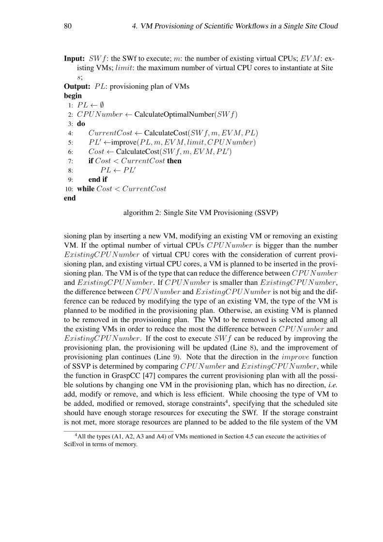
80 4. VM Provisioning of Scientific Workflows in a Single Site Cloud
Input: SWf : the SWf to execute; m: the number of existing virtual CPUs; EVM : ex-isting VMs; limit: the maximum number of virtual CPU cores to instantiate at Sites;
Output: PL: provisioning plan of VMsbegin
1: PL← ∅2: CPUNumber ← CalculateOptimalNumber(SWf)3: do4: CurrentCost← CalculateCost(SWf,m,EVM,PL)5: PL′ ←improve(PL,m,EVM, limit, CPUNumber)6: Cost← CalculateCost(SWf,m,EVM,PL′)7: if Cost < CurrentCost then8: PL← PL′
9: end if10: while Cost < CurrentCostend
algorithm 2: Single Site VM Provisioning (SSVP)
sioning plan by inserting a new VM, modifying an existing VM or removing an existingVM. If the optimal number of virtual CPUs CPUNumber is bigger than the numberExistingCPUNumber of virtual CPU cores with the consideration of current provi-sioning plan, and existing virtual CPU cores, a VM is planned to be inserted in the provi-sioning plan. The VM is of the type that can reduce the difference betweenCPUNumberand ExistingCPUNumber. If CPUNumber is smaller than ExistingCPUNumber,the difference between CPUNumber and ExistingCPUNumber is not big and the dif-ference can be reduced by modifying the type of an existing VM, the type of the VM isplanned to be modified in the provisioning plan. Otherwise, an existing VM is plannedto be removed in the provisioning plan. The VM to be removed is selected among allthe existing VMs in order to reduce the most the difference between CPUNumber andExistingCPUNumber. If the cost to execute SWf can be reduced by improving theprovisioning plan, the provisioning will be updated (Line 8), and the improvement ofprovisioning plan continues (Line 9). Note that the direction in the improve functionof SSVP is determined by comparing CPUNumber and ExistingCPUNumber, whilethe function in GraspCC [47] compares the current provisioning plan with all the possi-ble solutions by changing one VM in the provisioning plan, which has no direction, i.e.add, modify or remove, and which is less efficient. While choosing the type of VM tobe added, modified or removed, storage constraints4, specifying that the scheduled siteshould have enough storage resources for executing the SWf. If the storage constraintis not met, more storage resources are planned to be added to the file system of the VM
4All the types (A1, A2, A3 and A4) of VMs mentioned in Section 4.5 can execute the activities ofSciEvol in terms of memory.
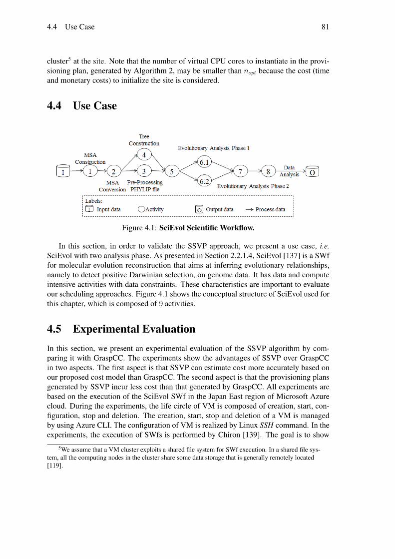
4.4 Use Case 81
cluster5 at the site. Note that the number of virtual CPU cores to instantiate in the provi-sioning plan, generated by Algorithm 2, may be smaller than nopt because the cost (timeand monetary costs) to initialize the site is considered.
4.4 Use Case
Figure 4.1: SciEvol Scientific Workflow.
In this section, in order to validate the SSVP approach, we present a use case, i.e.SciEvol with two analysis phase. As presented in Section 2.2.1.4, SciEvol [137] is a SWffor molecular evolution reconstruction that aims at inferring evolutionary relationships,namely to detect positive Darwinian selection, on genome data. It has data and computeintensive activities with data constraints. These characteristics are important to evaluateour scheduling approaches. Figure 4.1 shows the conceptual structure of SciEvol used forthis chapter, which is composed of 9 activities.
4.5 Experimental EvaluationIn this section, we present an experimental evaluation of the SSVP algorithm by com-paring it with GraspCC. The experiments show the advantages of SSVP over GraspCCin two aspects. The first aspect is that SSVP can estimate cost more accurately based onour proposed cost model than GraspCC. The second aspect is that the provisioning plansgenerated by SSVP incur less cost than that generated by GraspCC. All experiments arebased on the execution of the SciEvol SWf in the Japan East region of Microsoft Azurecloud. During the experiments, the life circle of VM is composed of creation, start, con-figuration, stop and deletion. The creation, start, stop and deletion of a VM is managedby using Azure CLI. The configuration of VM is realized by Linux SSH command. In theexperiments, the execution of SWfs is performed by Chiron [139]. The goal is to show
5We assume that a VM cluster exploits a shared file system for SWf execution. In a shared file sys-tem, all the computing nodes in the cluster share some data storage that is generally remotely located[119].
82 4. VM Provisioning of Scientific Workflows in a Single Site Cloud
Table 4.1: Parameters of different types of VMs. Type represents the type of VMs.vCPUs represents the number of virtual CPUs in a VM. RAM represents the size ofmemory in a VM. Disk represents the size of the hard disk in a VM. CC represents thecomputing capacity of VMs. MC represents Monetary Cost.
Type vCPUs RAM Disk CC MCA1 1 1.75 70 9.6 0.0604A2 2 3.5 135 19.2 0.1208A3 4 7 285 38.4 0.2416A4 8 14 605 76.8 0.4832
that SSVP is suitable to dynamic provisioning of VMs by making a good trade-off amongdifferent objectives for the execution of SWfs. Microsoft Azure provides 5 tiers of VM,which are basic tier, standard tier, optimized compute, performance optimized computeand compute intensive. Each tier of VM contains several types of VMs. In one Web do-main, users can provision different types of VMs at the same tier. In our experiments, weconsider 4 types, namely A1, A2, A3, and A4, in the standard tier. The features of theVM types are summarized in Table 4.1. In Azure, the time quantum is one minute. Inaddition, the average time to provision a VM is estimated as 2.9 minutes. Each VM usesLinux Ubuntu 12.04 (64-bit), and is configured with the necessary software for SciEvol.All VMs are configured to be accessed using Secure Shell (SSH).
Table 4.2: Workload Estimation.
ActivityNumber of Fasta Files
100 500 1000Estimated Workload (in GFLOP)
1 1440 10416 208332 384 2778 55563 576 4167 83334 1440 10416 20833
6.1 5760 41667 833346.2 10560 76389 1527786.3 49920 361111 7222226.4 59520 430556 8611116.5 75840 548611 10972226.6 202560 1465278 29305568 6720 48611 97222
In the experiments, we use 100, 500, 1000 fasta files generated from the data stored ina genome database [7][9]. The programs used are: mafft (version 7.221) for Activity 1,ReadSeq 2.1.26 for Activity 2, raxmhpc (7.2.8 alpha) for Activity 4, pamlX1.3.1 for Ac-tivities 6.1−6.2, in-house script for Activity 3 and Activity 8, and Activity 5 and Activity
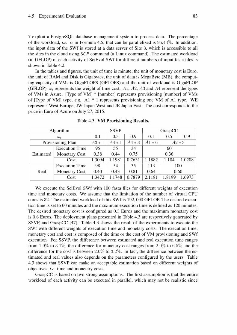
4.5 Experimental Evaluation 83
7 exploit a PostgreSQL database management system to process data. The percentageof the workload, i.e. α in Formula 4.5, that can be parallelized is 96.43%. In addition,the input data of the SWf is stored at a data server of Site 3, which is accessible to allthe sites in the cloud using SCP command (a Linux command). The estimated workload(in GFLOP) of each activity of SciEvol SWf for different numbers of input fasta files isshown in Table 4.2.
In the tables and figures, the unit of time is minute, the unit of monetary cost is Euro,the unit of RAM and Disk is Gigabytes, the unit of data is MegaByte (MB), the comput-ing capacity of VMs is GigaFLOPS (GFLOPS) and the unit of workload is GigaFLOP(GFLOP). ωt represents the weight of time cost. A1, A2, A3 and A4 represent the typesof VMs in Azure. [Type of VM] * [number] represents provisioning [number] of VMsof [Type of VM] type, e.g. A1 * 1 represents provisioning one VM of A1 type. WErepresents West Europe; JW Japan West and JE Japan East. The cost corresponds to theprice in Euro of Azure on July 27, 2015.
Table 4.3: VM Provisioning Results.
Algorithm SSVP GraspCCωt 0.1 0.5 0.9 0.1 0.5 0.9
Provisioning Plan A3 ∗ 1 A4 ∗ 1 A4 ∗ 3 A1 ∗ 6 A2 ∗ 3
EstimatedExecution Time 95 55 34 60Monetary Cost 0.38 0.44 0.75 0.36
Cost 1.3094 1.1981 0.7631 1.1882 1.104 1.0208
RealExecution Time 98 54 35 113 100Monetary Cost 0.40 0.43 0.81 0.64 0.60
Cost 1.3472 1.1748 0.7879 2.1181 1.8199 1.6973
We execute the SciEvol SWf with 100 fasta files for different weights of executiontime and monetary costs. We assume that the limitation of the number of virtual CPUcores is 32. The estimated workload of this SWf is 192, 000 GFLOP. The desired execu-tion time is set to 60 minutes and the maximum execution time is defined as 120 minutes.The desired monetary cost is configured as 0.3 Euros and the maximum monetary costis 0.6 Euros. The deployment plans presented in Table 4.3 are respectively generated bySSVP, and GraspCC [47]. Table 4.3 shows the result of the experiments to execute theSWf with different weights of execution time and monetary costs. The execution time,monetary cost and cost is composed of the time or the cost of VM provisioning and SWfexecution. For SSVP, the difference between estimated and real execution time rangesfrom 1.9% to 3.1%, the difference for monetary cost ranges from 2.0% to 6.5% and thedifference for the cost is between 2.0% to 3.2%. In fact, the difference between the es-timated and real values also depends on the parameters configured by the users. Table4.3 shows that SSVP can make an acceptable estimation based on different weights ofobjectives, i.e. time and monetary costs.
GraspCC is based on two strong assumptions. The first assumption is that the entireworkload of each activity can be executed in parallel, which may not be realistic since
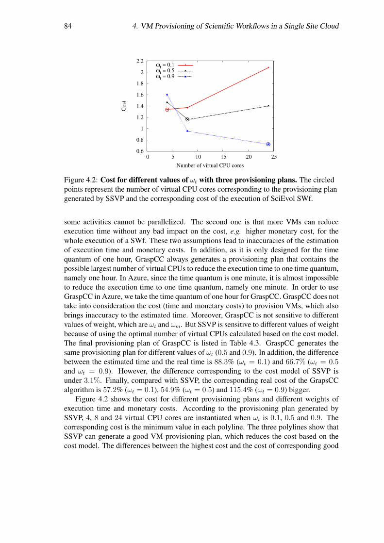
84 4. VM Provisioning of Scientific Workflows in a Single Site Cloud
0.6
0.8
1
1.2
1.4
1.6
1.8
2
2.2
0 5 10 15 20 25
Cost
Number of virtual CPU cores
ωt = 0.1ωt = 0.5ωt = 0.9
Figure 4.2: Cost for different values of ωt with three provisioning plans. The circledpoints represent the number of virtual CPU cores corresponding to the provisioning plangenerated by SSVP and the corresponding cost of the execution of SciEvol SWf.
some activities cannot be parallelized. The second one is that more VMs can reduceexecution time without any bad impact on the cost, e.g. higher monetary cost, for thewhole execution of a SWf. These two assumptions lead to inaccuracies of the estimationof execution time and monetary costs. In addition, as it is only designed for the timequantum of one hour, GraspCC always generates a provisioning plan that contains thepossible largest number of virtual CPUs to reduce the execution time to one time quantum,namely one hour. In Azure, since the time quantum is one minute, it is almost impossibleto reduce the execution time to one time quantum, namely one minute. In order to useGraspCC in Azure, we take the time quantum of one hour for GraspCC. GraspCC does nottake into consideration the cost (time and monetary costs) to provision VMs, which alsobrings inaccuracy to the estimated time. Moreover, GraspCC is not sensitive to differentvalues of weight, which are ωt and ωm. But SSVP is sensitive to different values of weightbecause of using the optimal number of virtual CPUs calculated based on the cost model.The final provisioning plan of GraspCC is listed in Table 4.3. GraspCC generates thesame provisioning plan for different values of ωt (0.5 and 0.9). In addition, the differencebetween the estimated time and the real time is 88.3% (ωt = 0.1) and 66.7% (ωt = 0.5and ωt = 0.9). However, the difference corresponding to the cost model of SSVP isunder 3.1%. Finally, compared with SSVP, the corresponding real cost of the GrapsCCalgorithm is 57.2% (ωt = 0.1), 54.9% (ωt = 0.5) and 115.4% (ωt = 0.9) bigger.
Figure 4.2 shows the cost for different provisioning plans and different weights ofexecution time and monetary costs. According to the provisioning plan generated bySSVP, 4, 8 and 24 virtual CPU cores are instantiated when ωt is 0.1, 0.5 and 0.9. Thecorresponding cost is the minimum value in each polyline. The three polylines show thatSSVP can generate a good VM provisioning plan, which reduces the cost based on thecost model. The differences between the highest cost and the cost of corresponding good
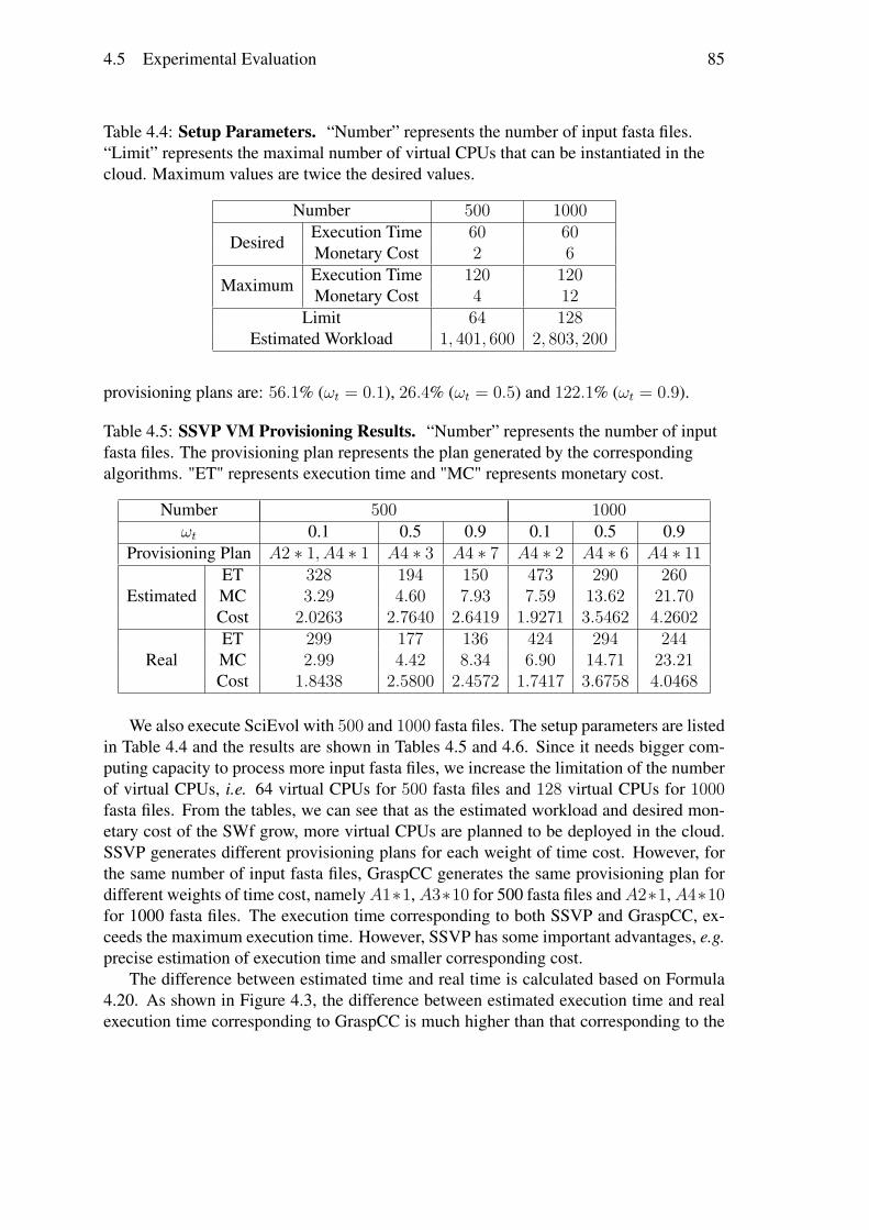
4.5 Experimental Evaluation 85
Table 4.4: Setup Parameters. “Number” represents the number of input fasta files.“Limit” represents the maximal number of virtual CPUs that can be instantiated in thecloud. Maximum values are twice the desired values.
Number 500 1000
DesiredExecution Time 60 60Monetary Cost 2 6
MaximumExecution Time 120 120Monetary Cost 4 12
Limit 64 128Estimated Workload 1, 401, 600 2, 803, 200
provisioning plans are: 56.1% (ωt = 0.1), 26.4% (ωt = 0.5) and 122.1% (ωt = 0.9).
Table 4.5: SSVP VM Provisioning Results. “Number” represents the number of inputfasta files. The provisioning plan represents the plan generated by the correspondingalgorithms. "ET" represents execution time and "MC" represents monetary cost.
Number 500 1000ωt 0.1 0.5 0.9 0.1 0.5 0.9
Provisioning Plan A2 ∗ 1, A4 ∗ 1 A4 ∗ 3 A4 ∗ 7 A4 ∗ 2 A4 ∗ 6 A4 ∗ 11
EstimatedET 328 194 150 473 290 260MC 3.29 4.60 7.93 7.59 13.62 21.70Cost 2.0263 2.7640 2.6419 1.9271 3.5462 4.2602
RealET 299 177 136 424 294 244MC 2.99 4.42 8.34 6.90 14.71 23.21Cost 1.8438 2.5800 2.4572 1.7417 3.6758 4.0468
We also execute SciEvol with 500 and 1000 fasta files. The setup parameters are listedin Table 4.4 and the results are shown in Tables 4.5 and 4.6. Since it needs bigger com-puting capacity to process more input fasta files, we increase the limitation of the numberof virtual CPUs, i.e. 64 virtual CPUs for 500 fasta files and 128 virtual CPUs for 1000fasta files. From the tables, we can see that as the estimated workload and desired mon-etary cost of the SWf grow, more virtual CPUs are planned to be deployed in the cloud.SSVP generates different provisioning plans for each weight of time cost. However, forthe same number of input fasta files, GraspCC generates the same provisioning plan fordifferent weights of time cost, namelyA1∗1,A3∗10 for 500 fasta files andA2∗1,A4∗10for 1000 fasta files. The execution time corresponding to both SSVP and GraspCC, ex-ceeds the maximum execution time. However, SSVP has some important advantages, e.g.precise estimation of execution time and smaller corresponding cost.
The difference between estimated time and real time is calculated based on Formula4.20. As shown in Figure 4.3, the difference between estimated execution time and realexecution time corresponding to GraspCC is much higher than that corresponding to the

86 4. VM Provisioning of Scientific Workflows in a Single Site Cloud
Table 4.6: GraspCC VM Provisioning Results. “Number” represents the number ofinput fasta files. The provisioning plan represents the plan generated by the correspond-ing algorithms.
Number 500 1000Provisioning Plan A1 ∗ 1, A3 ∗ 10 A2 ∗ 1, A4 ∗ 10
EstimatedExecution Time 60 60Monetary Cost 2.48 4.95
Cost 1.2144 1.1191 1.0238 0.8429 0.9127 0.9825
RealExecution Time 166 257Monetary Cost 6.19 22.43
Cost 3.06 2.93 2.80 3.79 4.01 4.23
1
10
100
100 500 1000
Diff
eren
ce(%
)
Number of fasta files
GraspCC ωt = 0.1GraspCC ωt = 0.5GraspCC ωt = 0.9
SSVP ωt = 0.1SSVP ωt = 0.5SSVP ωt = 0.9
Figure 4.3: Difference between estimated time and real time.
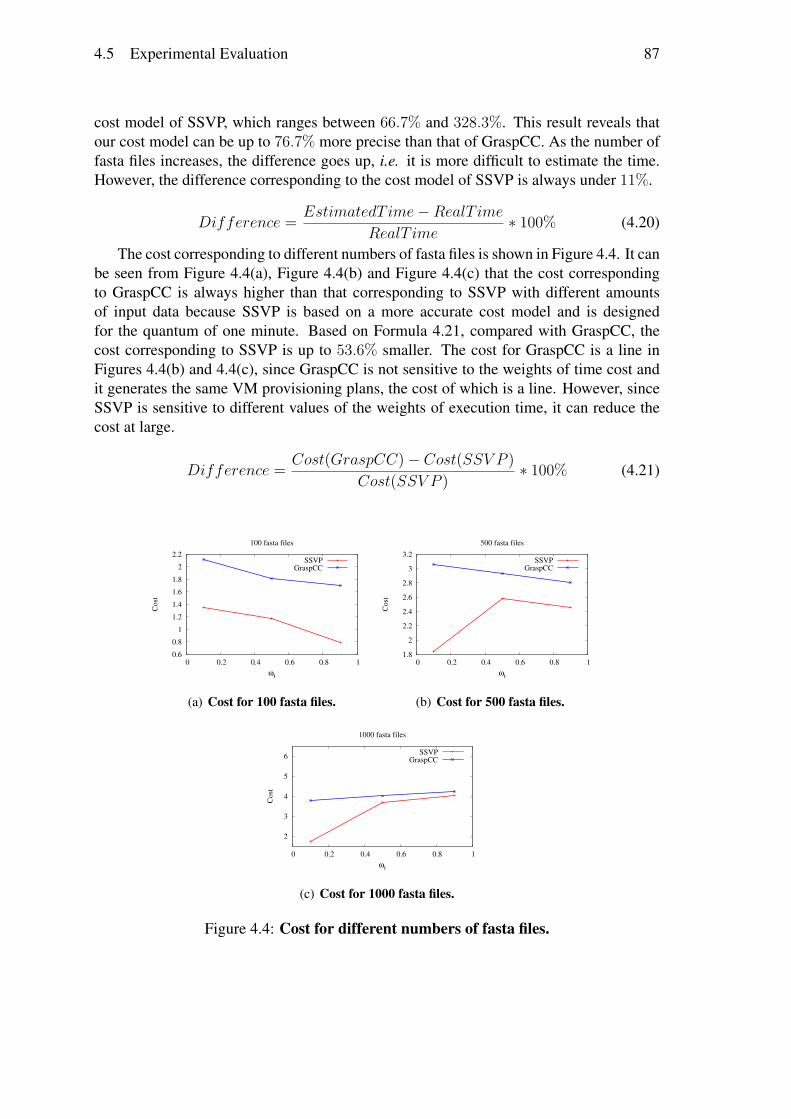
4.5 Experimental Evaluation 87
cost model of SSVP, which ranges between 66.7% and 328.3%. This result reveals thatour cost model can be up to 76.7% more precise than that of GraspCC. As the number offasta files increases, the difference goes up, i.e. it is more difficult to estimate the time.However, the difference corresponding to the cost model of SSVP is always under 11%.
Difference = EstimatedT ime−RealT imeRealT ime
∗ 100% (4.20)
The cost corresponding to different numbers of fasta files is shown in Figure 4.4. It canbe seen from Figure 4.4(a), Figure 4.4(b) and Figure 4.4(c) that the cost correspondingto GraspCC is always higher than that corresponding to SSVP with different amountsof input data because SSVP is based on a more accurate cost model and is designedfor the quantum of one minute. Based on Formula 4.21, compared with GraspCC, thecost corresponding to SSVP is up to 53.6% smaller. The cost for GraspCC is a line inFigures 4.4(b) and 4.4(c), since GraspCC is not sensitive to the weights of time cost andit generates the same VM provisioning plans, the cost of which is a line. However, sinceSSVP is sensitive to different values of the weights of execution time, it can reduce thecost at large.
Difference = Cost(GraspCC)− Cost(SSV P )Cost(SSV P ) ∗ 100% (4.21)
0.60.8
11.21.41.61.8
22.2
0 0.2 0.4 0.6 0.8 1
Cost
ωt
100 fasta files
SSVPGraspCC
(a) Cost for 100 fasta files.
1.8
2
2.2
2.4
2.6
2.8
3
3.2
0 0.2 0.4 0.6 0.8 1
Cost
ωt
500 fasta files
SSVPGraspCC
(b) Cost for 500 fasta files.
2
3
4
5
6
0 0.2 0.4 0.6 0.8 1
Cost
ωt
1000 fasta files
SSVPGraspCC
(c) Cost for 1000 fasta files.
Figure 4.4: Cost for different numbers of fasta files.
88 4. VM Provisioning of Scientific Workflows in a Single Site Cloud
From the experimental results, we can get the conclusion that SSVP can generatebetter VM provisioning plans than GraspCC because of accurate cost estimation of thecost model.
4.6 ConclusionIn this chapter, we proposed a new VM provisioning approach, namely SSVP, to generateVM provisioning plans for SWf execution with multiple objectives in a single site cloud.The cost model aims at minimizing two costs: execution time and monetary costs. Weused a real SWf that is SciEvol, with real data from the bioinformatics domain as a usecase. We evaluated our approaches by executing SciEvol in Microsoft Azure cloud. Theresults show the provisioning approach (SSVP) generates better provisioning plans fordifferent weights of time cost to execute a SWf at a site, compared with other existingapproaches, namely GraspCC. The advantage of SSVP can be up to 53.6%. In addition,our cost model can estimate the cost within an acceptable error limit and it is 76.7% moreprecise than that of GraspCC.
Chapter 5
Multi-Objective Scheduling of ScientificWorkflows in a Multisite Cloud
Clouds appear as appropriate infrastructures for executing Scientific Workflows (SWfs).A cloud is typically made of several sites (or data centers), each with its own resourcesand data. Thus, it becomes important to be able to execute some SWfs at more than onecloud site because of the geographical distribution of data or available resources amongdifferent cloud sites. Therefore, a major problem is how to execute a SWf in a multisitecloud, while reducing execution time and monetary costs. This chapter is based on [117]and [118].
Section 5.3 defines the problems for SWf scheduling. In this chapter, we propose ageneral solution based on multi-objective scheduling in order to execute SWfs in a mul-tisite cloud. The solution consists of a multi-objective cost model including executiontime and monetary costs and ActGreedy, a multisite scheduling approach. Section 5.4describes the system architecture for SWf execution in a multisite cloud. Section 5.5 de-scribes our multi-objective optimization approach and Section 5.6 describes our schedul-ing approaches including the SciEvol SWf use case, the approaches for SWf partitioningand three scheduling approaches, i.e. ActGreedy, LocBased and SGreedy. Then, Section5.7 is our experimental evaluation based on the execution of the SciEvol SWf in MicrosoftAzure cloud. The results reveal that our scheduling approach significantly outperformstwo adapted baseline algorithms (which we propose by adapting two existing algorithms)and the scheduling time is reasonable compared with genetic and brute-force algorithms.
5.1 Overview and MotivationsLarge-scale in silico scientific experiments typically take advantage of SWfs to modeldata operations such as loading input data, data processing, data analysis, and aggregat-ing output data. SWfs enable scientists to model the data processing of these experimentsas a graph, in which vertices represent data processing activities and edges represent de-pendencies between them. A SWf is the assembly of scientific data processing activities
89

90 5. Multi-Objective Scheduling of Scientific Workflows in a Multisite Cloud
with data dependencies among them [57]. An activity is the description of a piece ofwork that forms a logical step within a SWf representation [120]. Since SWf activitiesmay process big data, we can exploit data parallelism whereby one activity correspondsto several executable tasks, each working in parallel on a different part of the input data.
In order to execute SWfs efficiently, SWfMSs typically exploit High PerformanceComputing (HPC) resources in a cluster, grid or cloud environment. Because of virtuallyinfinite resources, diverse scalable services, stable quality of service and flexible paymentpolicies, clouds have become an interesting solution for SWf execution. In particular, theuser of Virtual Machines (VMs) makes it easy to deal with elasticity and workloads thatchange rapidly. A cloud is typically made of several sites (or data centers), each with itsown resources and data. Thus, in order to use more resources than available at a single siteor to access data at different sites, SWfs could also be executed in a distributed mannerat different sites. Nowadays, the computing resources or data of a cloud provider suchas Amazon or Microsoft are distributed at different sites and should be used during theexecution of SWfs. As a result, a multisite cloud is an appealing solution for large scaleSWf execution. As defined in [119], a multisite cloud is a cloud with multiple data centers,each at a different location (possibly in a different region) and being explicitly accessibleto cloud users, typically in the data center close to them for performance reasons.
To enable SWf execution in a multisite cloud, the execution of each activity should bescheduled to a corresponding cloud site (or site for short). Then, the scheduling problemis to decide where to execute the activities. In general, to map the execution of activitiesto distributed computing resources is an NP-hard problem [195]. The objectives can be toreduce execution time or monetary cost, to maximize performance, reliability etc. SinceSWf execution may take a long time and cost much money, the scheduling problem mayhave multiple objectives, i.e. multi-objective. Thus, the multisite scheduling problemmust take into account the impact of resources distributed at different sites, e.g. differentbandwidths and data distribution at different sites, and different prices for VMs.
In this chapter, we propose a general solution based on multi-objective schedulingin order to execute SWfs in a multisite cloud. The solution includes a multi-objectivecost model for multisite SWf execution and ActGreedy, a multisite scheduling approach.The cost model includes two objectives, namely reducing execution time and monetarycosts, under stored data constraints, which specify that some data should not be moved,because it is either too big or for proprietary reasons. Although useful for fixing someactivities, these constraints do not reduce much the complexity of activity scheduling.We consider a homogeneous cloud environment, i.e. from single provider. The caseof federated clouds (with multiple cloud providers) is beyond the scope of this chapterand relatively new to cloud users [176]. ActGreedy handles multiple objectives, namelyreducing execution time and monetary costs. In order to schedule a SWf in a multisitecloud, the SWf should be partitioned to SWf fragments, which can be executed at a singlesite. Each fragment can be scheduled by ActGreedy to the site that yields the minimumcost among all available sites. When a fragment is scheduled to a site, the execution ofits associated activities is scheduled to the site. ActGreedy is based on our dynamic VMprovisioning algorithm, i.e. SSVP (see Section 4.3), which generates VM provisioning

5.2 Related Work 91
plans for the execution of fragments with minimum cost at the scheduled site based ona cost model. The cost model is used to estimate the cost of the execution of SWfs [52]according to a scheduling plan, which defines the schedule of fragments to execution sites.A VM provisioning plan defines how to provision VMs. For instance, it determines thetypes, corresponding number and the order of VMs to provision, for the execution of afragment. The VM type determines some parameters such as the number of virtual CPUs,the size of memory and the default storage size of hard disk. The main contributions ofthis chapter are:
1. The design of a multi-objective cost model that includes execution time and mone-tary costs, to estimate the cost of executing SWfs in a multisite cloud.
2. ActGreedy multisite scheduling algorithm that uses the cost model and SSVP toschedule and execute SWfs in a multisite cloud.
3. An extensive experimental evaluation, based on the implementation of our approachin Microsoft Azure, and using a real SWf use case (SciEvol [137], a bioinformat-ics SWf for molecular evolution reconstruction) that shows the advantages of ourapproach, compared with baseline algorithms.
5.2 Related WorkTo the best of authors’ knowledge, there is no solution to execute SWfs in a multisite cloudenvironment that takes into account both multiple objectives and dynamic VM provision-ing. The related work either focuses on static VM provisioning [65], single objective[22, 125, 154, 168, 177, 196, 186, 67, 125, 122] or single site execution [52, 70, 158].Static VM provisioning refers to the use of the existing VMs (before execution) for SWfexecution without changing the types of VMs during execution. However, existing costmodels are not suitable for the SWfs that have a big part of the sequential workload. Forinstance, the dynamic approach proposed in [47] ignores the sequential part of the SWfand the cost of provisioning VMs, which may generate VM provisioning plans that yieldhigh cost.
Many solutions for SWf scheduling [22, 125, 154, 168, 177, 196] focus on a singleobjective, i.e. reducing execution time. These solutions address the scheduling problemin a single site cloud. Classic heuristics have been used in scheduling algorithms, suchas HEFT [186], min-min [67], max-min [67] and Opportunistic Load Balancing (OLB)[125], but they only address the single objective. Furthermore, they are designed for staticcomputing resources in grid or cluster environments. In contrast, our algorithm handlesmultiple objectives, which are reducing execution time and monetary costs, with dynamicVM provisioning support. Although some general heuristics, e.g. genetic algorithms[186], can generate near optimal scheduling plans, it is not always feasible to designalgorithms for every possible optimization problem [186] and it is not trivial to configureparameters for the problem. In addition, it may take much time to generate scheduling

92 5. Multi-Objective Scheduling of Scientific Workflows in a Multisite Cloud
plans. A brute-force method can generate an optimal scheduling plan, but its complexityis very high.
Some multi-objective scheduling techniques [52, 70, 158] have been proposed. How-ever, they do not take the distribution of resources at different sites into consideration, sothey are not suitable for a multisite environment. De Oliveira et al. [52] propose a greedyscheduling approach for the execution of SWfs at a single site. However, this approach isnot appropriate for multisite execution of SWfs as it schedules the most suitable activitiesto each VM, which may incur transferring of big data. Rodriguez and Buyya [158] intro-duce an algorithm for scheduling dynamic bags of tasks and dynamic VM provisioningfor the execution of SWfs with multiple objectives in a single site cloud. Rather than us-ing real execution, they simulate the execution of SWfs , thus missing the heterogeneityamong the activities of the same SWf, to evaluate their proposed approaches. In real SWfexecution, the activities generally correspond to different programs to process data. How-ever, in simulations of SWf execution, the activities are typically made homogeneous,namely, they correspond to the same program. Different from the existing approaches,our approach is suitable for multisite execution and is evaluated by executing a real-lifeSWf on a multisite cloud (Azure).
Some scheduling techniques have been proposed for the multisite cloud, yet focusingon a single objective, i.e. reducing execution time. For instance, Liu et al. [122] presenta workflow partitioning approach and data location based scheduling approach. But thisapproach does not take monetary cost into consideration. Our approach uses an a pri-ori method, where preference information is given by users and then the best solution isproduced. Our approach is based on a multi-objective scheduling algorithm focusing onminimizing a weighted sum of objectives. The advantage of such approach is that it isautomatically guided by predetermined weights while the disadvantage is that it is hard todetermine the right values for the weights [29]. In contrast, a posteriori methods producea Pareto front of solutions without predetermined values [29]. Each solution is better thanthe others with respect to at least one objective and users can choose one from the pro-duced solutions. However, this method requires users to pick the most suitable solution.In this chapter, we assume that users have a clear idea of the importance of objectives, andthey can determine the value for the weight of each objective. One advantage of usinga priori method is that we can produce optimal or near optimal solutions without userinterference at run-time. When we are using the method of Pareto front, several solutionsmay be produced to be chosen by the user. Finally, when the weight of each objectiveis positive, the minimum of the sum is already a Pareto optimal solution [198] [128] andour proposed approach can generate a Pareto optimal or near-optimal solution with thepredefined weights. Therefore, we do not consider a posteriori methods.
The existing cost models for generating VM provisioning plans [47] are not suitablefor SWfs in multisite environments [52, 161] and they do not consider sequential work-load in SWfs. Our cost model is based on the cost model presented in Section 4.2, whichdoes consider the cost to provision VMs and the sequential parts of the workload in SWfexecution. Furthermore, the cost model also works for multisite SWf execution.
Duan et al. [65] propose a multisite multi-objective scheduling approach with consid-

5.3 Problem Definition 93
eration of different bandwidths in a multisite environment. However, it is only suitablefor static computing resources. In our approach, our scheduling approach is based on amore precise cost model and our SSVP algorithmfor dynamic VM provisioning.
5.3 Problem DefinitionThis section introduces some important terms, i.e. SWf, SWf fragment and multisitecloud and defines the scheduling problem in the multisite cloud.
A SWf is described as a Directed Acyclic Graph (DAG) denoted by W (V ,E). LetV = {v1, v2, ..., vn} be a set of vertices, which are associated with the scientific dataprocessing activities and E = {ei,j: vi, vj ∈ V and vj consumes the output data of vi } bea set of edges that correspond to dependencies between activities in V . Activity vj is thefollowing activity of Activity vi and Activity vi is a preceding activity of Activity vj . Thedependencies can be data or control dependencies. Compared to data dependencies, fewerdata are transferred in control dependencies. The transferred data in a control dependencyis the configuration parameters for activity execution while the transferred data in a datadependency is the input data to be processed by the following activity. The activity thatprocesses control parameters is a control activity. Since the control activity takes littletime to execute, we assume that a control activity has no workload. In addition, we assumethat the data stored at a specific site may not be allowed to be transferred to other sitesbecause of proprietary or big amounts of data, which is denoted as stored data constraint.If an activity needs to read the data from the stored data located at a specific site, thisactivity is denoted as fixed activity.
A large-scale SWf and its input data can be partitioned into several fragments [39][122]. Thus, a SWf can be described as the assembly of fragments and fragment de-pendencies, i.e. W (WF , FE) where WF = {wf1, wf2, ..., wfn} represents a set offragments connected by dependencies in the set FE = {fei,j: wfi, wfj ∈ WF and wfjconsumes the output data of wfi}. A fragment dependency fei,j represents that fragmentwfj processes the output data of fragment wfi. fei,j is the input dependency of wfj andoutput dependency of wfi. A fragment can be denoted by wf (V , E, D). V representsthe activities, E represents the dependencies and D represents the input data of the SWffragment.
We denote the SWf execution environment by a configured multisite cloud1 MS(S),which consists of a set of sites S. A multisite cloud configuration defines the instancesof VMs and storage resources for cloud users in a multisite cloud. One site si ∈ S iscomposed of a set of Web domains. A Web domain contains a set of VMs, shared storageresources, and stored data. In this chapter, we assume that one site contains only one Webdomain for the execution of a SWf. We assume that the available VMs for the executionof SWfs in a multisite cloud have the same virtual CPUs, i.e. the virtual CPUs have thesame computing capacity, but the number of virtual CPUs in each VM may be different.
1The multisite cloud environment configured for the quota of resources that can be used by a clouduser.

94 5. Multi-Objective Scheduling of Scientific Workflows in a Multisite Cloud
In addition, we assume that the price to instantiate VMs of the same type are the same atthe same site while the prices at different sites can be different. The price is the monetarycost to use a VM during a time quantum (the quantum varies according to the cloudprovider, e.g. one hour or one minute). Time quantum is the smallest possible discreteunit to calculate the cost of using a VM. For instance, if the time quantum is one minuteand the price of a VM is 0.5 dollar per hour, the cost to use the VM for the time period ofT (T ≥ N − 1 minutes and T < N minutes) will be N∗0.5
60 dollars.Scheduling fragments requires choosing a site to execute a fragment, i.e. mapping
each fragment to an execution site. A fragment scheduling plan defines the map of frag-ments and sites. When a fragment is scheduled at a site, the activities of the fragment arealso scheduled at that site. Based on a multi-objective cost model, the problem we addresshas the following form [146]:
min(Cost(Sch(SWf, S)))subject to
stored data constraintThe decision variable is Schedule(wf, s), which is defined as
Schedule(wf, s) ={
1 if Fragment wf is scheduled at Site s0 otherwise
Thus, the scheduling problem is, given a multi-objective cost model, how to generate afragment scheduling plan Sch(SWf, S), for which the corresponding SWf execution hasminimum Cost(Sch(SWf, S)) while respecting the stored data constraints Const(data)with data ∈ input(SWf). The cost is the value calculated based on formulas definedin a cost model, e.g. Formulas 5.1 and 5.2, which depends on a scheduling plan and VMprovisioning plans at scheduled sites. In the scheduling plan, for each Fragment wf andsite s, only if Fragment wf is scheduled at Site s, the decision variable is 1; otherwise,the variable is 0. One fragment can be scheduled at only one site. The search space ofscheduling plans contains all the possible scheduling plans, i.e. for any combination ofwf and s, we can find a scheduling plan in the search space that contains the decisionvariable Schedule(wf, s) = 1. If the cost is composed of just one objective, the problemis a single objective optimization problem. Otherwise, the problem is a multi-objectiveproblem. The cost model is detailed in Section 5.5.1. In this chapter, we use SSVP(see Section 4.3) to generate VM provisioning plans. The stored data constraints can berepresented as a matrix (as the one presented below), and its cell values are known beforeexecution, where each row ai represents an activity, each column sj represents a cloudsite, and (ai, sj) = 1 means that ai needs to read the data stored at sj .
s1 s2 s3a1 1 0 0a2 0 0 1a3 0 1 0
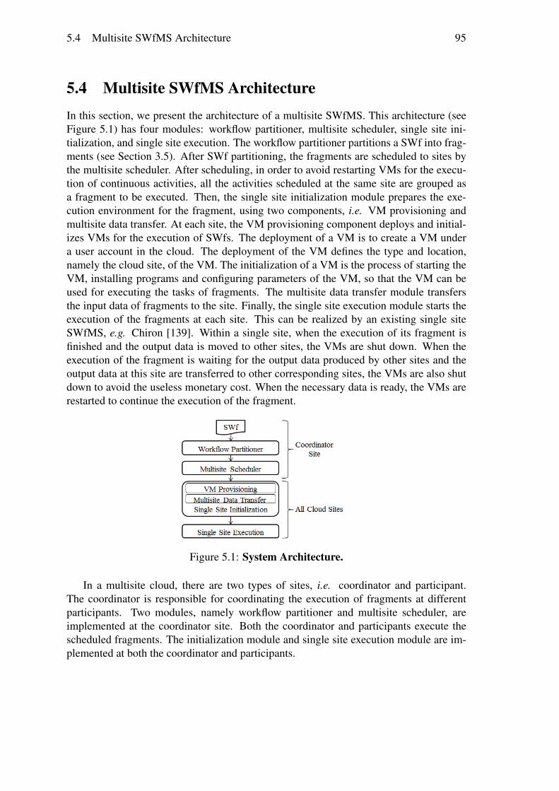
5.4 Multisite SWfMS Architecture 95
5.4 Multisite SWfMS ArchitectureIn this section, we present the architecture of a multisite SWfMS. This architecture (seeFigure 5.1) has four modules: workflow partitioner, multisite scheduler, single site ini-tialization, and single site execution. The workflow partitioner partitions a SWf into frag-ments (see Section 3.5). After SWf partitioning, the fragments are scheduled to sites bythe multisite scheduler. After scheduling, in order to avoid restarting VMs for the execu-tion of continuous activities, all the activities scheduled at the same site are grouped asa fragment to be executed. Then, the single site initialization module prepares the exe-cution environment for the fragment, using two components, i.e. VM provisioning andmultisite data transfer. At each site, the VM provisioning component deploys and initial-izes VMs for the execution of SWfs. The deployment of a VM is to create a VM undera user account in the cloud. The deployment of the VM defines the type and location,namely the cloud site, of the VM. The initialization of a VM is the process of starting theVM, installing programs and configuring parameters of the VM, so that the VM can beused for executing the tasks of fragments. The multisite data transfer module transfersthe input data of fragments to the site. Finally, the single site execution module starts theexecution of the fragments at each site. This can be realized by an existing single siteSWfMS, e.g. Chiron [139]. Within a single site, when the execution of its fragment isfinished and the output data is moved to other sites, the VMs are shut down. When theexecution of the fragment is waiting for the output data produced by other sites and theoutput data at this site are transferred to other corresponding sites, the VMs are also shutdown to avoid the useless monetary cost. When the necessary data is ready, the VMs arerestarted to continue the execution of the fragment.
Figure 5.1: System Architecture.
In a multisite cloud, there are two types of sites, i.e. coordinator and participant.The coordinator is responsible for coordinating the execution of fragments at differentparticipants. Two modules, namely workflow partitioner and multisite scheduler, areimplemented at the coordinator site. Both the coordinator and participants execute thescheduled fragments. The initialization module and single site execution module are im-plemented at both the coordinator and participants.
96 5. Multi-Objective Scheduling of Scientific Workflows in a Multisite Cloud
5.5 Multi-objective OptimizationThis section focuses on multi-objective optimization, which is composed of a multi-objective cost model, used to estimate the cost of executing SWfs in a multisite cloudand a cost estimation method for the scheduling process.
5.5.1 Multi-objective Cost ModelWe propose a multi-objective cost model, which is composed of time cost, i.e. executiontime, and monetary cost for the execution of SWfs. In order to choose a good schedulingplan, we need a cost model to estimate the cost of executing a SWf in a multisite cloud. Acost model is composed of a set of formulas to estimate the cost of the execution of SWfs[52] according to a scheduling plan. It is generally implemented in the scheduling moduleand under a specific execution environment. In the case of this chapter, the executionenvironment is a multisite cloud. Our proposed cost model is an extension of the modelproposed in [52] and [161]. In addition, the cost model is also used to calculate the realcost by replacing estimated parameters by real values obtained from the real execution inthe evaluation part, i.e. Section 5.7.
The cost of executing a SWf can be defined by:
Cost(Sch(SWf, S)) =ωt ∗Time(Sch(SWf, S))
DesiredT ime
+ ωm ∗Money(Sch(SWf, S))
DesiredMoney
(5.1)
, where DesiredT ime represents the desired execution time to execute the SWf andDesiredMoney is the desired monetary cost for the execution. Both DesiredT ime andDesiredMoney are configured by the users. Note that these may be unfeasible to obtainfor the execution of the SWf. We take the desired execution time and monetary costs intoconsideration in the cost model while the real execution time and monetary costs maybe bigger or smaller depending on the real execution environment. Time(SWf) andMoney(SWf) is the real execution time and real monetary cost for the execution of theSWf. ωt and ωm represent the weights for execution time and monetary costs, which arepositive.
However, it is difficult to estimate the execution time and monetary costs for the wholeSWf even with a scheduling plan according to Formula 5.1 since it is hard to generatea VM provisioning plan for each site with global desired execution time and monetarycosts. As shown in Formula 5.2, we decompose the cost model as the sum of the cost ofexecuting each fragment.
Cost(Sch(SWf, S)) =Schedule(wfi,sj)=1∑
wfi∈SWf
Cost(wfi, sj) (5.2)
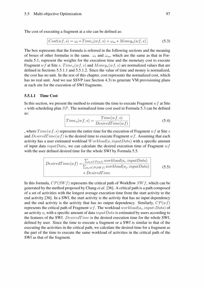
5.5 Multi-objective Optimization 97
The cost of executing a fragment at a site can be defined as:
Cost(wf, s) = ωt ∗ Timen(wf, s) + ωm ∗Moneyn(wf, s) (5.3)
The box represents that the formula is referred in the following sections and the meaningof boxes of other formulas is the same. ωt and ωm, which are the same as that in For-mula 5.1, represent the weights for the execution time and the monetary cost to executeFragment wf at Site s. Timen(wf, s) and Moneyn(wf, s) are normalized values that aredefined in Sections 5.5.1.1 and 5.5.1.2. Since the value of time and money is normalized,the cost has no unit. In the rest of this chapter, cost represents the normalized cost, whichhas no real unit. And we use SSVP (see Section 4.3) to generate VM provisioning plansat each site for the execution of SWf fragments.
5.5.1.1 Time Cost
In this section, we present the method to estimate the time to execute Fragment wf at Sites with scheduling plan SP . The normalized time cost used in Formula 5.3 can be definedas:
Timen(wf, s) = Time(wf, s)DesiredT ime(wf) (5.4)
, where Time(wf, s) represents the entire time for the execution of Fragment wf at Site sand DesiredT ime(wf) is the desired time to execute Fragment wf . Assuming that eachactivity has a user estimated workload Workload(a, inputData) with a specific amountof input data inputData, we can calculate the desired execution time of Fragment wfwith the user defined desired time for the whole SWf by Formula 5.5.
DesiredT ime(wf) =∑ai∈CP (wf) workload(ai, inputData)∑aj∈CP (SWf) workload(aj, inputData)∗DesiredT ime
(5.5)
In this formula, CP (SWf) represents the critical path of Workflow SWf , which can begenerated by the method proposed by Chang et al. [36]. A critical path is a path composedof a set of activities with the longest average execution time from the start activity to theend activity [36]. In a SWf, the start activity is the activity that has no input dependencyand the end activity is the activity that has no output dependency. Similarly, CP (wf)represents the critical path of Fragment wf . The workload workload(ai, input-Data) ofan activity ai with a specific amount of data inputData is estimated by users according tothe features of the SWf. DesiredT ime is the desired execution time for the whole SWf,defined by user. Since the time to execute a fragment or a SWf is similar to that of theexecuting the activities in the critical path, we calculate the desired time for a fragment asthe part of the time to execute the same workload of activities in the critical path of theSWf as that of the fragment.

98 5. Multi-Objective Scheduling of Scientific Workflows in a Multisite Cloud
In order to execute Fragment wf at Site s, the system needs to initialize the corre-sponding execution site, to transfer the corresponding input data of Fragment wf to Sites and to run the program in the VMs of the site. The initialization of the site is explainedin Section 5.4. This way, the entire time for the execution of Fragment wf at Site s canbe estimated by the following formula:
Time(wf, s) =InitializationT ime(wf, s)+ TransferT ime(wf, s)+ ExecutionT ime(wf, s)
(5.6)
, where s represents the site to execute Fragment wf according to the scheduling planSP , InitializationT ime represents the time to initialize Site s, TransferT ime is thetime to transfer input data from other sites to Site s and ExecutionT ime is the time toexecute the fragment. In order to simplify the problem, we ignore the cost (both timecost and monetary cost) to restart VMs at a site to wait for the output data produced byother sites. In this formula, the time to wait for the input data produced by the activitiesexecuted at another site (Site so) is not considered since this time is considered in that ofthe fragment executed at Site so.
The multisite SWfMS needs to provision m (determined by SSVP) VMs to executeFragment wf at a single site. As explained in Section 5.4, to provision a VM is to deployand to initialize a VM at a cloud site. The time to provision the VMs at a single site isestimated by Formula 4.4.
The time for data transfer is the sum of the time to transfer input data stored in othersites to Site s. The data transfer time can be estimated by formula 5.7.
TransferT ime(wf, s) =∑si 6=s
DataTransferAmount(wf, si)DataTransferRate(si, s)
(5.7)
DataTransferAmount(wf, si) is the amount of input data of Fragment wf stored atSite si, which is defined later (see Formula 5.8). DataTransferRate(si, s) representsthe data transfer rate between Site si and Site s, which can be roughly obtained by mea-suring the amount of data transferred by Linux SCP command during a specific period oftime between two VMs located at the two sites.
We assume that the amount of input data for each dependency is estimated by the user.The amount of data to be transferred from another site (si) to the site (s) to execute thefragment can be estimated by Formula 5.8.
DataTransferAmount(wf, si)
=∑aj∈wf
ak∈activities(si)∑ak∈preceding(aj)
AmountOfData(ek,j)(5.8)
where preceding(aj) represents the preceding activities of Activity aj at Site so. si repre-
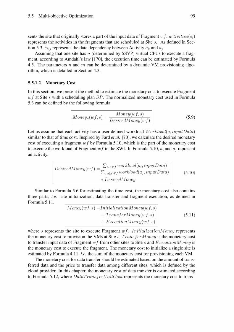
5.5 Multi-objective Optimization 99
sents the site that originally stores a part of the input data of Fragment wf . activities(si)represents the activities in the fragments that are scheduled at Site si. As defined in Sec-tion 5.3, ek,j represents the data dependency between Activity ak and aj .
Assuming that one site has n (determined by SSVP) virtual CPUs to execute a frag-ment, according to Amdahl’s law [170], the execution time can be estimated by Formula4.5. The parameters n and m can be determined by a dynamic VM provisioning algo-rithm, which is detailed in Section 4.3.
5.5.1.2 Monetary Cost
In this section, we present the method to estimate the monetary cost to execute Fragmentwf at Site s with a scheduling plan SP . The normalized monetary cost used in Formula5.3 can be defined by the following formula:
Moneyn(wf, s) = Money(wf, s)DesiredMoney(wf) (5.9)
Let us assume that each activity has a user defined workload Workload(a, inputData)similar to that of time cost. Inspired by Fard et al. [70], we calculate the desired monetarycost of executing a fragment wf by Formula 5.10, which is the part of the monetary costto execute the workload of Fragment wf in the SWf. In Formula 5.10, ai and aj representan activity.
DesiredMoney(wf) =∑ai∈wf workload(ai, inputData)∑aj∈SWf workload(aj, inputData)∗DesiredMoney
(5.10)
Similar to Formula 5.6 for estimating the time cost, the monetary cost also containsthree parts, i.e. site initialization, data transfer and fragment execution, as defined inFormula 5.11.
Money(wf, s) =InitializationMoney(wf, s)+ TransferMoney(wf, s)+ ExecutionMoney(wf, s)
(5.11)
where s represents the site to execute Fragment wf . InitializationMoney representsthe monetary cost to provision the VMs at Site s, TransferMoney is the monetary costto transfer input data of Fragment wf from other sites to Site s and ExecutionMoney isthe monetary cost to execute the fragment. The monetary cost to initialize a single site isestimated by Formula 4.11, i.e. the sum of the monetary cost for provisioning each VM.
The monetary cost for data transfer should be estimated based on the amount of trans-ferred data and the price to transfer data among different sites, which is defined by thecloud provider. In this chapter, the monetary cost of data transfer is estimated accordingto Formula 5.12, where DataTransferUnitCost represents the monetary cost to trans-
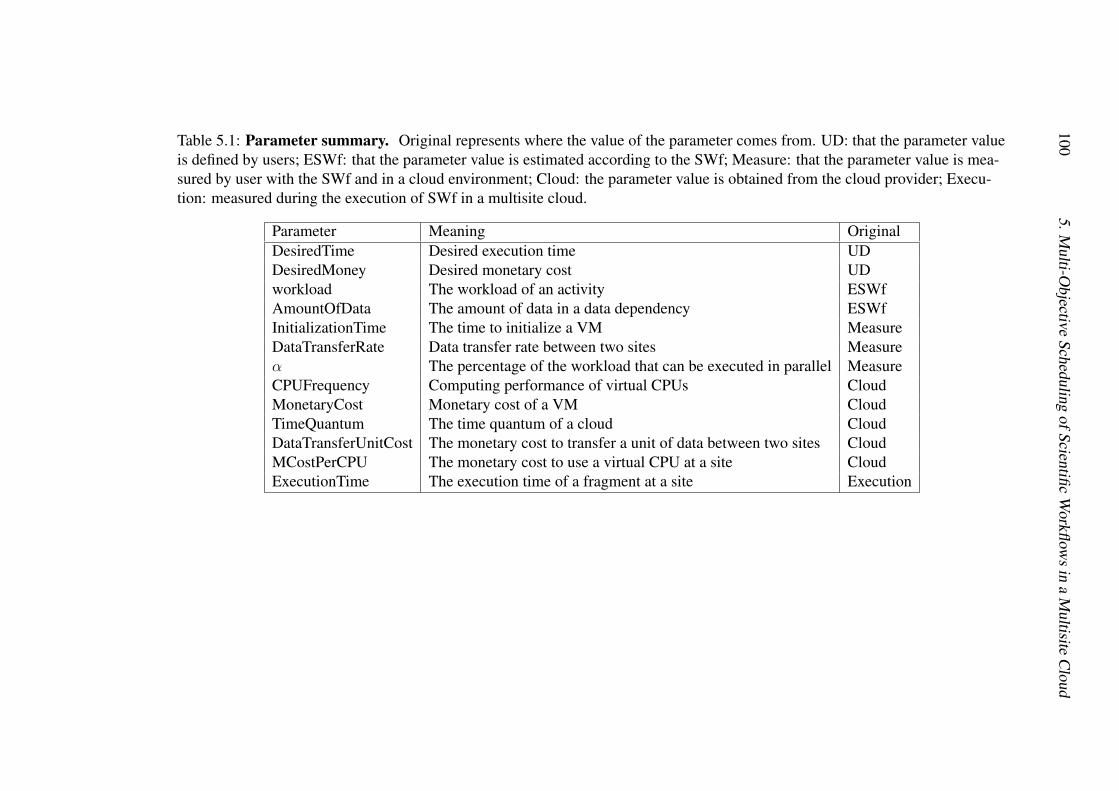
1005.M
ulti-Objective
SchedulingofScientific
Workflow
sin
aM
ultisiteC
loud
Table 5.1: Parameter summary. Original represents where the value of the parameter comes from. UD: that the parameter valueis defined by users; ESWf: that the parameter value is estimated according to the SWf; Measure: that the parameter value is mea-sured by user with the SWf and in a cloud environment; Cloud: the parameter value is obtained from the cloud provider; Execu-tion: measured during the execution of SWf in a multisite cloud.
Parameter Meaning OriginalDesiredTime Desired execution time UDDesiredMoney Desired monetary cost UDworkload The workload of an activity ESWfAmountOfData The amount of data in a data dependency ESWfInitializationTime The time to initialize a VM MeasureDataTransferRate Data transfer rate between two sites Measureα The percentage of the workload that can be executed in parallel MeasureCPUFrequency Computing performance of virtual CPUs CloudMonetaryCost Monetary cost of a VM CloudTimeQuantum The time quantum of a cloud CloudDataTransferUnitCost The monetary cost to transfer a unit of data between two sites CloudMCostPerCPU The monetary cost to use a virtual CPU at a site CloudExecutionTime The execution time of a fragment at a site Execution
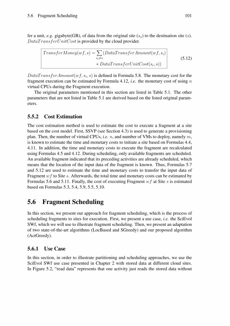
5.6 Fragment Scheduling 101
fer a unit, e.g. gigabyte(GB), of data from the original site (so) to the destination site (s).DataTransferUnitCost is provided by the cloud provider.
TransferMoney(wf, s) =∑si 6=s
(DataTransferAmount(wf, si)
∗DataTransferUnitCost(si, s))(5.12)
DataTransferAmount(wf, si, s) is defined in Formula 5.8. The monetary cost for thefragment execution can be estimated by Formula 4.12, i.e. the monetary cost of using nvirtual CPUs during the Fragment execution.
The original parameters mentioned in this section are listed in Table 5.1. The otherparameters that are not listed in Table 5.1 are derived based on the listed original param-eters.
5.5.2 Cost EstimationThe cost estimation method is used to estimate the cost to execute a fragment at a sitebased on the cost model. First, SSVP (see Section 4.3) is used to generate a provisioningplan. Then, the number of virtual CPUs, i.e. n, and number of VMs to deploy, namely m,is known to estimate the time and monetary costs to initiate a site based on Formulas 4.4,4.11. In addition, the time and monetary costs to execute the fragment are recalculatedusing Formulas 4.5 and 4.12. During scheduling, only available fragments are scheduled.An available fragment indicated that its preceding activities are already scheduled, whichmeans that the location of the input data of the fragment is known. Thus, Formulas 5.7and 5.12 are used to estimate the time and monetary costs to transfer the input data ofFragment wf to Site s. Afterwards, the total time and monetary costs can be estimated byFormulas 5.6 and 5.11. Finally, the cost of executing Fragment wf at Site s is estimatedbased on Formulas 5.3, 5.4, 5.9, 5.5, 5.10.
5.6 Fragment SchedulingIn this section, we present our approach for fragment scheduling, which is the process ofscheduling fragments to sites for execution. First, we present a use case, i.e. the SciEvolSWf, which we will use to illustrate fragment scheduling. Then, we present an adaptationof two state-of-the-art algorithms (LocBased and SGreedy) and our proposed algorithm(ActGreedy).
5.6.1 Use CaseIn this section, in order to illustrate partitioning and scheduling approaches, we use theSciEvol SWf use case presented in Chapter 2 with stored data at different cloud sites.In Figure 5.2, “read data” represents that one activity just reads the stored data without
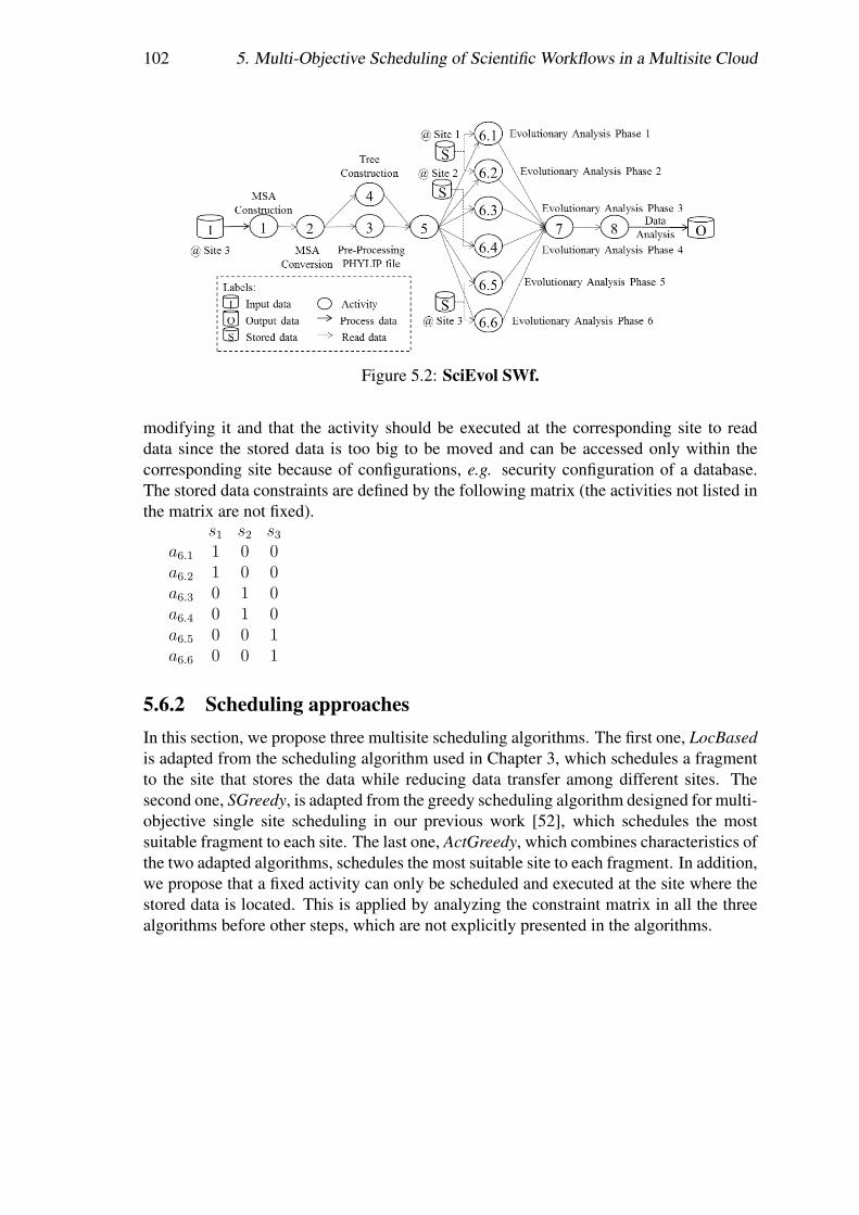
102 5. Multi-Objective Scheduling of Scientific Workflows in a Multisite Cloud
Figure 5.2: SciEvol SWf.
modifying it and that the activity should be executed at the corresponding site to readdata since the stored data is too big to be moved and can be accessed only within thecorresponding site because of configurations, e.g. security configuration of a database.The stored data constraints are defined by the following matrix (the activities not listed inthe matrix are not fixed).
s1 s2 s3a6.1 1 0 0a6.2 1 0 0a6.3 0 1 0a6.4 0 1 0a6.5 0 0 1a6.6 0 0 1
5.6.2 Scheduling approachesIn this section, we propose three multisite scheduling algorithms. The first one, LocBasedis adapted from the scheduling algorithm used in Chapter 3, which schedules a fragmentto the site that stores the data while reducing data transfer among different sites. Thesecond one, SGreedy, is adapted from the greedy scheduling algorithm designed for multi-objective single site scheduling in our previous work [52], which schedules the mostsuitable fragment to each site. The last one, ActGreedy, which combines characteristics ofthe two adapted algorithms, schedules the most suitable site to each fragment. In addition,we propose that a fixed activity can only be scheduled and executed at the site where thestored data is located. This is applied by analyzing the constraint matrix in all the threealgorithms before other steps, which are not explicitly presented in the algorithms.

5.6 Fragment Scheduling 103
Figure 5.3: SWf partitioning and data location based scheduling. The number repre-sents the relative (compared with the input data) amount of output data for correspond-ing activities.
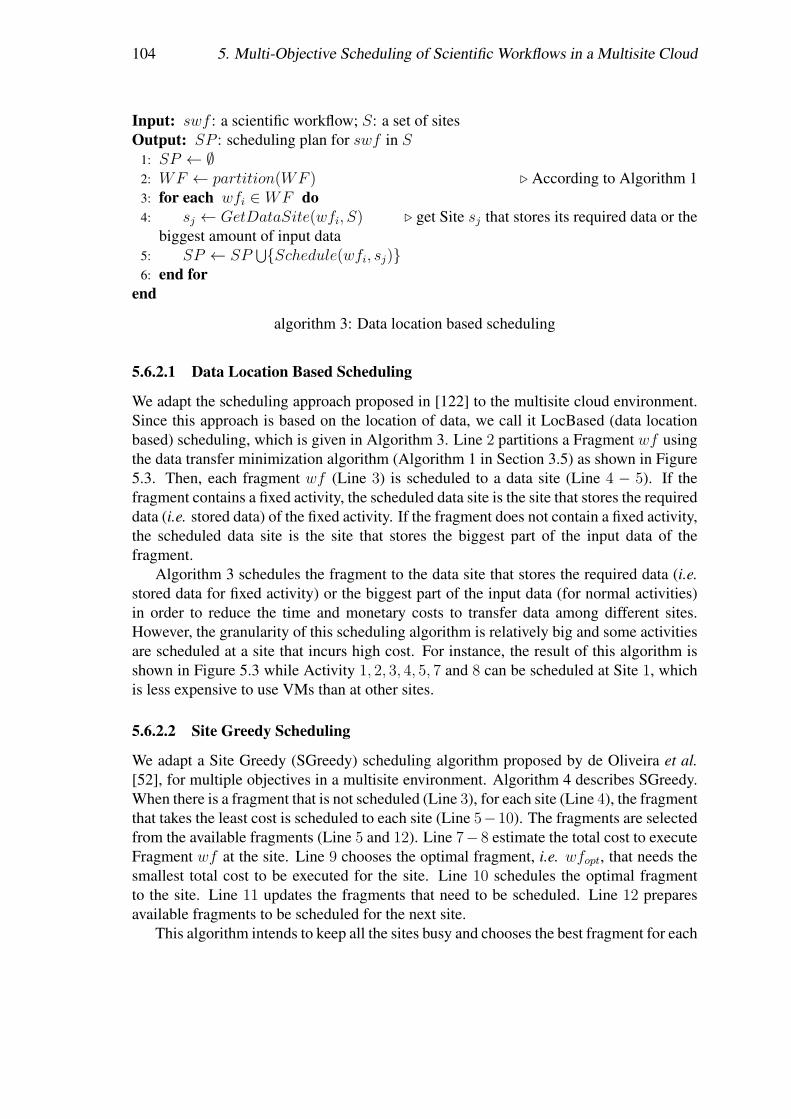
104 5. Multi-Objective Scheduling of Scientific Workflows in a Multisite Cloud
Input: swf : a scientific workflow; S: a set of sitesOutput: SP : scheduling plan for swf in S
1: SP ← ∅2: WF ← partition(WF ) . According to Algorithm 13: for each wfi ∈ WF do4: sj ← GetDataSite(wfi, S) . get Site sj that stores its required data or the
biggest amount of input data5: SP ← SP
⋃{Schedule(wfi, sj)}6: end for
end
algorithm 3: Data location based scheduling
5.6.2.1 Data Location Based Scheduling
We adapt the scheduling approach proposed in [122] to the multisite cloud environment.Since this approach is based on the location of data, we call it LocBased (data locationbased) scheduling, which is given in Algorithm 3. Line 2 partitions a Fragment wf usingthe data transfer minimization algorithm (Algorithm 1 in Section 3.5) as shown in Figure5.3. Then, each fragment wf (Line 3) is scheduled to a data site (Line 4 − 5). If thefragment contains a fixed activity, the scheduled data site is the site that stores the requireddata (i.e. stored data) of the fixed activity. If the fragment does not contain a fixed activity,the scheduled data site is the site that stores the biggest part of the input data of thefragment.
Algorithm 3 schedules the fragment to the data site that stores the required data (i.e.stored data for fixed activity) or the biggest part of the input data (for normal activities)in order to reduce the time and monetary costs to transfer data among different sites.However, the granularity of this scheduling algorithm is relatively big and some activitiesare scheduled at a site that incurs high cost. For instance, the result of this algorithm isshown in Figure 5.3 while Activity 1, 2, 3, 4, 5, 7 and 8 can be scheduled at Site 1, whichis less expensive to use VMs than at other sites.
5.6.2.2 Site Greedy Scheduling
We adapt a Site Greedy (SGreedy) scheduling algorithm proposed by de Oliveira et al.[52], for multiple objectives in a multisite environment. Algorithm 4 describes SGreedy.When there is a fragment that is not scheduled (Line 3), for each site (Line 4), the fragmentthat takes the least cost is scheduled to each site (Line 5−10). The fragments are selectedfrom the available fragments (Line 5 and 12). Line 7− 8 estimate the total cost to executeFragment wf at the site. Line 9 chooses the optimal fragment, i.e. wfopt, that needs thesmallest total cost to be executed for the site. Line 10 schedules the optimal fragmentto the site. Line 11 updates the fragments that need to be scheduled. Line 12 preparesavailable fragments to be scheduled for the next site.
This algorithm intends to keep all the sites busy and chooses the best fragment for each

5.6 Fragment Scheduling 105
Input: swf : a scientific workflow; S: a set of sitesOutput: SP : scheduling plan for swf in S
1: SP ← ∅2: WF ← partition(WF ) . According to activity encapsulation partitioning method3: while WF 6= ∅ do4: for each s ∈ S do5: WFA← GetAvailableFragments(WF )6: if WFA 6= ∅ then7: for each wf ∈ WFA do8: Cost[i]← EstimateCost(wf, s) . According to the cost estimation
method9: end for
10: wfopt ← GetFragment(s, Cost) . Get the fragment that takes theminimal cost for the execution at Site s
11: SP ← SP⋃{Schedule(wfopt, s)}
12: WF ← WF − wfopt13: WFA← GetAvailableFragments(WF )14: end if15: end for16: end whileend
algorithm 4: Site greedy scheduling
site. However, as shown in Figure 5.4, this algorithm may break the dataflow between theparent activity and child activity, which may incur high cost to transfer the data amongdifferent sites, e.g. Activities 1, 2, 3, 4, 7, 8. In addition, in order to avoid useless usage ofVMs at Site 1 and Site 2 during the execution of the SWf, the VMs are shut down afterfinishing the execution of the corresponding activities, and restarted for the followingactivities when the input data is ready. After executing Activities 1, 6.3 and 6.4, the VMsat Site 1 are shut down. The VMs at Site 2 are shut down after executing Activity 2.Since Activity 5 is a control activity, which takes little time to be executed, the VMs atSite 1 and 3 are not shut down after executing Activities 4 and 3. When the execution ofActivities 6.5 and 6.6 are to be finished, the VMs at Site 2 are restarted to continue theexecution (since the execution of Activities 6.5 and 6.6 may take more time because ofbig workload). This process may also incur high cost when there are many VMs to restart.
5.6.2.3 Activity Greedy Scheduling
Based on LocBased and SGreedy, we propose the ActGreedy (Activity Greedy) schedul-ing algorithm, which is described in Algorithm 5. In this algorithm, all the fragments ofa SWf are not scheduled, i.e. Sch(SWf, S) = ∅, at beginning. During the schedul-ing process, all the fragments are scheduled at a corresponding site, which takes the

106 5. Multi-Objective Scheduling of Scientific Workflows in a Multisite Cloud
Figure 5.4: Site greedy scheduling.
minimum cost, namely Sch(SWf, S) = {Schedule(wf, s)|wf ∈ SWf, s ∈ S} and∀ wf ∈ SWf,∃ Schedule(wf, s) ∈ Sch(SWf, S) while cost Cost(Schedule(wf, s))is the minimum compared to schedule Fragment wf to other sites. As a result, the costCost(Sch(SWf, S)) of executing a SWf in a multisite cloud is minimized. Similar toLocBased, ActGreedy schedules fragments of multiple activities. ActGreedy can sched-ule a pipeline of activities to reduce data transfer between different fragments, i.e. thepossible data transfer between different sites. As formally defined in [158], a pipelineis a group of activities with a one-to-one, sequential relationship between them. How-ever, ActGreedy is different from LocBased since it makes a trade-off between time andmonetary costs. Similar to SGreedy, ActGreedy schedules the available fragments, whilechoosing the best site for an available fragment instead of choosing the best fragment foran available site.
ActGreedy chooses the best site for each fragment. First, it partitions a SWf accordingto the activity encapsulation partitioning method (Line 3). Then, it groups the fragmentsof three types into bigger fragments to be scheduled (Line 6). The first type is a pipelineof activities. We use a recursive algorithm presented in [158] to find pipelines. Then,the fragments of corresponding activities of each pipeline are grouped into a fragment.If there are stored activities of different sites in a fragment of a pipeline, the fragment ispartitioned into several fragments by the data transfer minimization algorithm (Algorithm1) in the Group function. The second type is the control activities. If it has only onepreceding activity, a control activity is grouped into the fragment of its preceding activity.
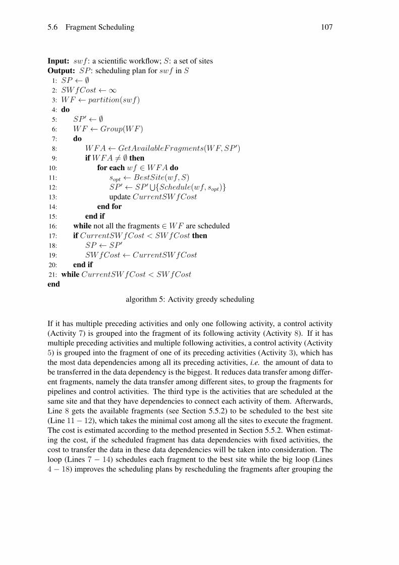
5.6 Fragment Scheduling 107
Input: swf : a scientific workflow; S: a set of sitesOutput: SP : scheduling plan for swf in S
1: SP ← ∅2: SWfCost←∞3: WF ← partition(swf)4: do5: SP ′ ← ∅6: WF ← Group(WF )7: do8: WFA← GetAvailableFragments(WF,SP ′)9: if WFA 6= ∅ then
10: for each wf ∈ WFA do11: sopt ← BestSite(wf, S)12: SP ′ ← SP ′
⋃{Schedule(wf, sopt)}13: update CurrentSWfCost14: end for15: end if16: while not all the fragments ∈ WF are scheduled17: if CurrentSWfCost < SWfCost then18: SP ← SP ′
19: SWfCost← CurrentSWfCost20: end if21: while CurrentSWfCost < SWfCostend
algorithm 5: Activity greedy scheduling
If it has multiple preceding activities and only one following activity, a control activity(Activity 7) is grouped into the fragment of its following activity (Activity 8). If it hasmultiple preceding activities and multiple following activities, a control activity (Activity5) is grouped into the fragment of one of its preceding activities (Activity 3), which hasthe most data dependencies among all its preceding activities, i.e. the amount of data tobe transferred in the data dependency is the biggest. It reduces data transfer among differ-ent fragments, namely the data transfer among different sites, to group the fragments forpipelines and control activities. The third type is the activities that are scheduled at thesame site and that they have dependencies to connect each activity of them. Afterwards,Line 8 gets the available fragments (see Section 5.5.2) to be scheduled to the best site(Line 11− 12), which takes the minimal cost among all the sites to execute the fragment.The cost is estimated according to the method presented in Section 5.5.2. When estimat-ing the cost, if the scheduled fragment has data dependencies with fixed activities, thecost to transfer the data in these data dependencies will be taken into consideration. Theloop (Lines 7 − 14) schedules each fragment to the best site while the big loop (Lines4 − 18) improves the scheduling plans by rescheduling the fragments after grouping the
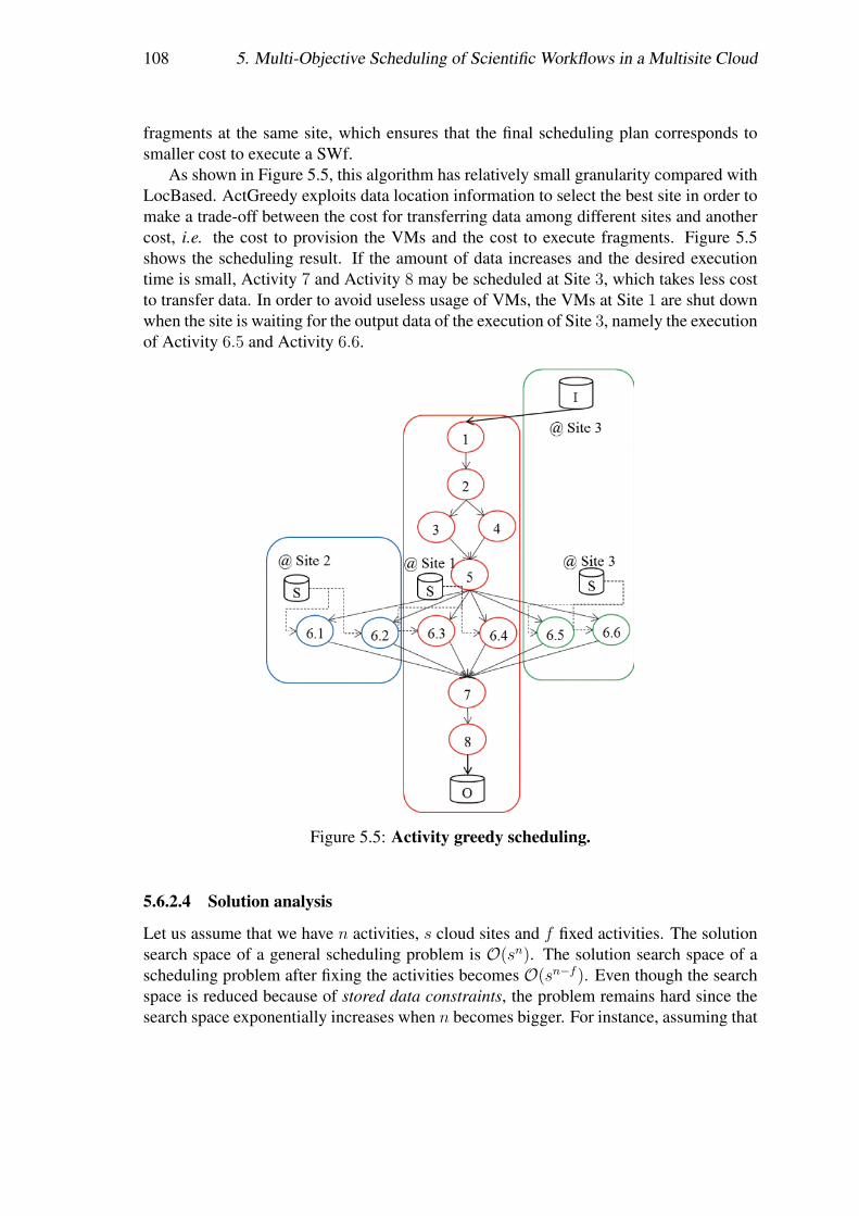
108 5. Multi-Objective Scheduling of Scientific Workflows in a Multisite Cloud
fragments at the same site, which ensures that the final scheduling plan corresponds tosmaller cost to execute a SWf.
As shown in Figure 5.5, this algorithm has relatively small granularity compared withLocBased. ActGreedy exploits data location information to select the best site in order tomake a trade-off between the cost for transferring data among different sites and anothercost, i.e. the cost to provision the VMs and the cost to execute fragments. Figure 5.5shows the scheduling result. If the amount of data increases and the desired executiontime is small, Activity 7 and Activity 8 may be scheduled at Site 3, which takes less costto transfer data. In order to avoid useless usage of VMs, the VMs at Site 1 are shut downwhen the site is waiting for the output data of the execution of Site 3, namely the executionof Activity 6.5 and Activity 6.6.
Figure 5.5: Activity greedy scheduling.
5.6.2.4 Solution analysis
Let us assume that we have n activities, s cloud sites and f fixed activities. The solutionsearch space of a general scheduling problem is O(sn). The solution search space of ascheduling problem after fixing the activities becomes O(sn−f ). Even though the searchspace is reduced because of stored data constraints, the problem remains hard since thesearch space exponentially increases when n becomes bigger. For instance, assuming that
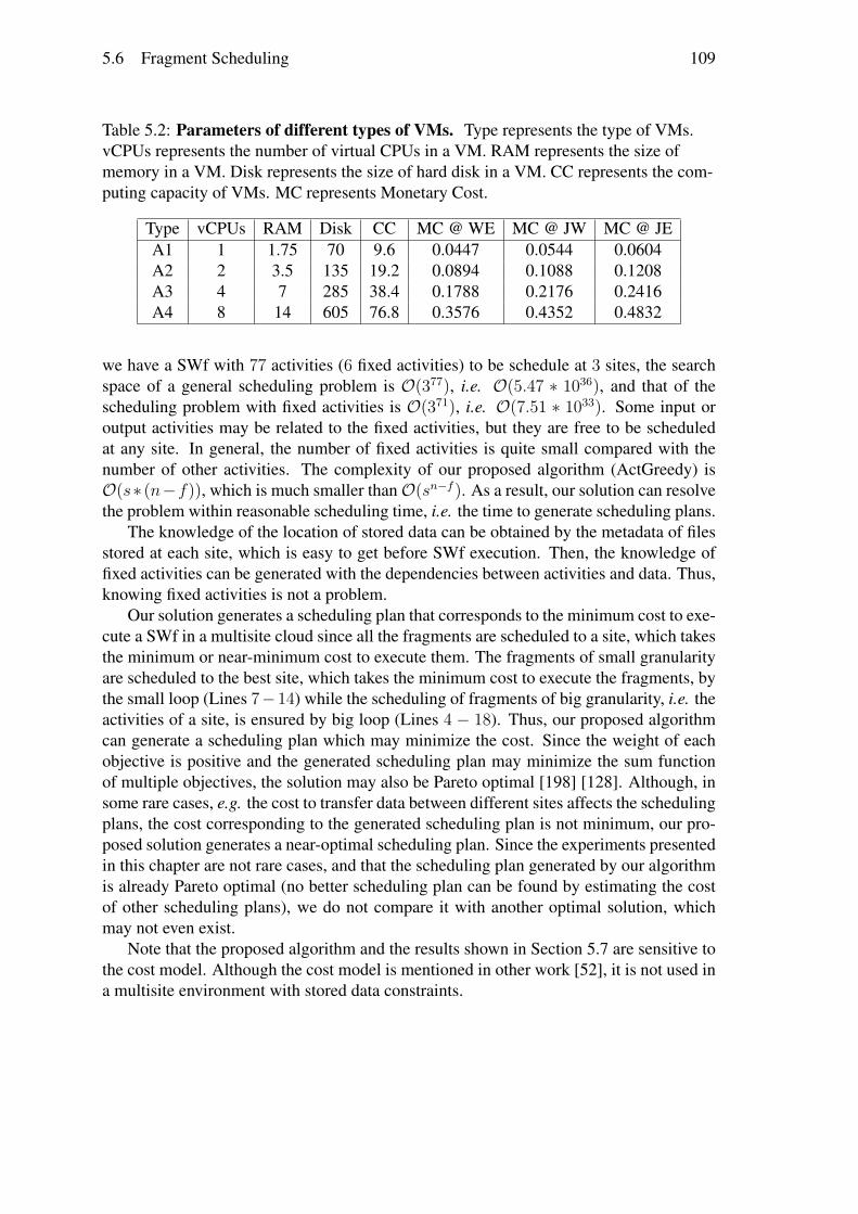
5.6 Fragment Scheduling 109
Table 5.2: Parameters of different types of VMs. Type represents the type of VMs.vCPUs represents the number of virtual CPUs in a VM. RAM represents the size ofmemory in a VM. Disk represents the size of hard disk in a VM. CC represents the com-puting capacity of VMs. MC represents Monetary Cost.
Type vCPUs RAM Disk CC MC @ WE MC @ JW MC @ JEA1 1 1.75 70 9.6 0.0447 0.0544 0.0604A2 2 3.5 135 19.2 0.0894 0.1088 0.1208A3 4 7 285 38.4 0.1788 0.2176 0.2416A4 8 14 605 76.8 0.3576 0.4352 0.4832
we have a SWf with 77 activities (6 fixed activities) to be schedule at 3 sites, the searchspace of a general scheduling problem is O(377), i.e. O(5.47 ∗ 1036), and that of thescheduling problem with fixed activities is O(371), i.e. O(7.51 ∗ 1033). Some input oroutput activities may be related to the fixed activities, but they are free to be scheduledat any site. In general, the number of fixed activities is quite small compared with thenumber of other activities. The complexity of our proposed algorithm (ActGreedy) isO(s∗ (n−f)), which is much smaller thanO(sn−f ). As a result, our solution can resolvethe problem within reasonable scheduling time, i.e. the time to generate scheduling plans.
The knowledge of the location of stored data can be obtained by the metadata of filesstored at each site, which is easy to get before SWf execution. Then, the knowledge offixed activities can be generated with the dependencies between activities and data. Thus,knowing fixed activities is not a problem.
Our solution generates a scheduling plan that corresponds to the minimum cost to exe-cute a SWf in a multisite cloud since all the fragments are scheduled to a site, which takesthe minimum or near-minimum cost to execute them. The fragments of small granularityare scheduled to the best site, which takes the minimum cost to execute the fragments, bythe small loop (Lines 7−14) while the scheduling of fragments of big granularity, i.e. theactivities of a site, is ensured by big loop (Lines 4 − 18). Thus, our proposed algorithmcan generate a scheduling plan which may minimize the cost. Since the weight of eachobjective is positive and the generated scheduling plan may minimize the sum functionof multiple objectives, the solution may also be Pareto optimal [198] [128]. Although, insome rare cases, e.g. the cost to transfer data between different sites affects the schedulingplans, the cost corresponding to the generated scheduling plan is not minimum, our pro-posed solution generates a near-optimal scheduling plan. Since the experiments presentedin this chapter are not rare cases, and that the scheduling plan generated by our algorithmis already Pareto optimal (no better scheduling plan can be found by estimating the costof other scheduling plans), we do not compare it with another optimal solution, whichmay not even exist.
Note that the proposed algorithm and the results shown in Section 5.7 are sensitive tothe cost model. Although the cost model is mentioned in other work [52], it is not used ina multisite environment with stored data constraints.
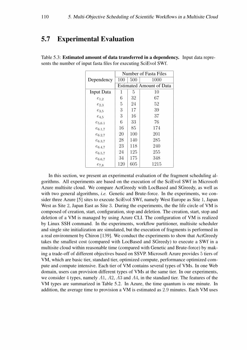
110 5. Multi-Objective Scheduling of Scientific Workflows in a Multisite Cloud
5.7 Experimental Evaluation
Table 5.3: Estimated amount of data transferred in a dependency. Input data repre-sents the number of input fasta files for executing SciEvol SWf.
DependencyNumber of Fasta Files
100 500 1000Estimated Amount of Data
Input Data 1 5 10e1,2 6 32 67e2,3 5 24 52e3,5 3 17 39e4,5 3 16 37e5,6.1 6 33 76e6.1,7 16 85 174e6.2,7 20 100 201e6.3,7 28 140 285e6.4,7 23 118 240e6.5,7 24 125 255e6.6,7 34 175 348e7,8 120 605 1215
In this section, we present an experimental evaluation of the fragment scheduling al-gorithms. All experiments are based on the execution of the SciEvol SWf in MicrosoftAzure multisite cloud. We compare ActGreedy with LocBased and SGreedy, as well aswith two general algorithms, i.e. Genetic and Brute-force. In the experiments, we con-sider three Azure [5] sites to execute SciEvol SWf, namely West Europe as Site 1, JapanWest as Site 2, Japan East as Site 3. During the experiments, the the life circle of VM iscomposed of creation, start, configuration, stop and deletion. The creation, start, stop anddeletion of a VM is managed by using Azure CLI. The configuration of VM is realizedby Linux SSH command. In the experiments, workflow partitioner, multisite schedulerand single site initialization are simulated, but the execution of fragments is performed ina real environment by Chiron [139]. We conduct the experiments to show that ActGreedytakes the smallest cost (compared with LocBased and SGreedy) to execute a SWf in amultisite cloud within reasonable time (compared with Genetic and Brute-force) by mak-ing a trade-off of different objectives based on SSVP. Microsoft Azure provides 5 tiers ofVM, which are basic tier, standard tier, optimized compute, performance optimized com-pute and compute intensive. Each tier of VM contains several types of VMs. In one Webdomain, users can provision different types of VMs at the same tier. In our experiments,we consider 4 types, namely A1, A2, A3 and A4, in the standard tier. The features of theVM types are summarized in Table 5.2. In Azure, the time quantum is one minute. Inaddition, the average time to provision a VM is estimated as 2.9 minutes. Each VM uses
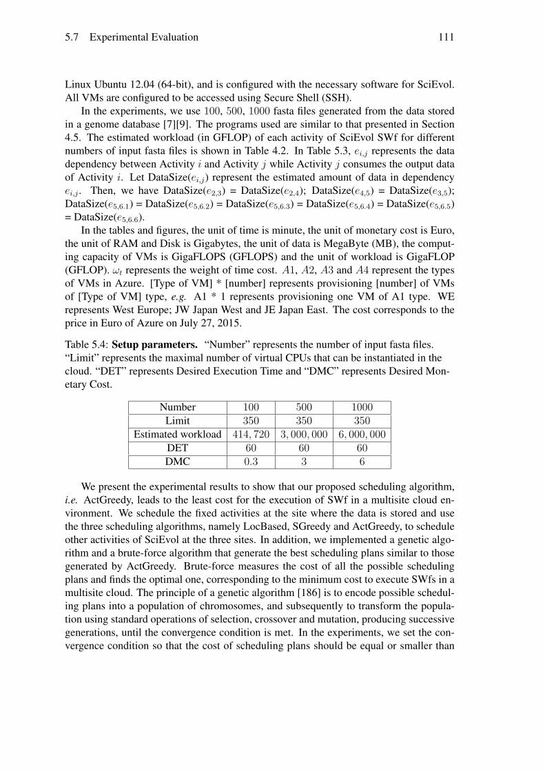
5.7 Experimental Evaluation 111
Linux Ubuntu 12.04 (64-bit), and is configured with the necessary software for SciEvol.All VMs are configured to be accessed using Secure Shell (SSH).
In the experiments, we use 100, 500, 1000 fasta files generated from the data storedin a genome database [7][9]. The programs used are similar to that presented in Section4.5. The estimated workload (in GFLOP) of each activity of SciEvol SWf for differentnumbers of input fasta files is shown in Table 4.2. In Table 5.3, ei,j represents the datadependency between Activity i and Activity j while Activity j consumes the output dataof Activity i. Let DataSize(ei,j) represent the estimated amount of data in dependencyei,j . Then, we have DataSize(e2,3) = DataSize(e2,4); DataSize(e4,5) = DataSize(e3,5);DataSize(e5,6.1) = DataSize(e5,6.2) = DataSize(e5,6.3) = DataSize(e5,6.4) = DataSize(e5,6.5)= DataSize(e5,6.6).
In the tables and figures, the unit of time is minute, the unit of monetary cost is Euro,the unit of RAM and Disk is Gigabytes, the unit of data is MegaByte (MB), the comput-ing capacity of VMs is GigaFLOPS (GFLOPS) and the unit of workload is GigaFLOP(GFLOP). ωt represents the weight of time cost. A1, A2, A3 and A4 represent the typesof VMs in Azure. [Type of VM] * [number] represents provisioning [number] of VMsof [Type of VM] type, e.g. A1 * 1 represents provisioning one VM of A1 type. WErepresents West Europe; JW Japan West and JE Japan East. The cost corresponds to theprice in Euro of Azure on July 27, 2015.
Table 5.4: Setup parameters. “Number” represents the number of input fasta files.“Limit” represents the maximal number of virtual CPUs that can be instantiated in thecloud. “DET” represents Desired Execution Time and “DMC” represents Desired Mon-etary Cost.
Number 100 500 1000Limit 350 350 350
Estimated workload 414, 720 3, 000, 000 6, 000, 000DET 60 60 60DMC 0.3 3 6
We present the experimental results to show that our proposed scheduling algorithm,i.e. ActGreedy, leads to the least cost for the execution of SWf in a multisite cloud en-vironment. We schedule the fixed activities at the site where the data is stored and usethe three scheduling algorithms, namely LocBased, SGreedy and ActGreedy, to scheduleother activities of SciEvol at the three sites. In addition, we implemented a genetic algo-rithm and a brute-force algorithm that generate the best scheduling plans similar to thosegenerated by ActGreedy. Brute-force measures the cost of all the possible schedulingplans and finds the optimal one, corresponding to the minimum cost to execute SWfs in amultisite cloud. The principle of a genetic algorithm [186] is to encode possible schedul-ing plans into a population of chromosomes, and subsequently to transform the popula-tion using standard operations of selection, crossover and mutation, producing successivegenerations, until the convergence condition is met. In the experiments, we set the con-vergence condition so that the cost of scheduling plans should be equal or smaller than
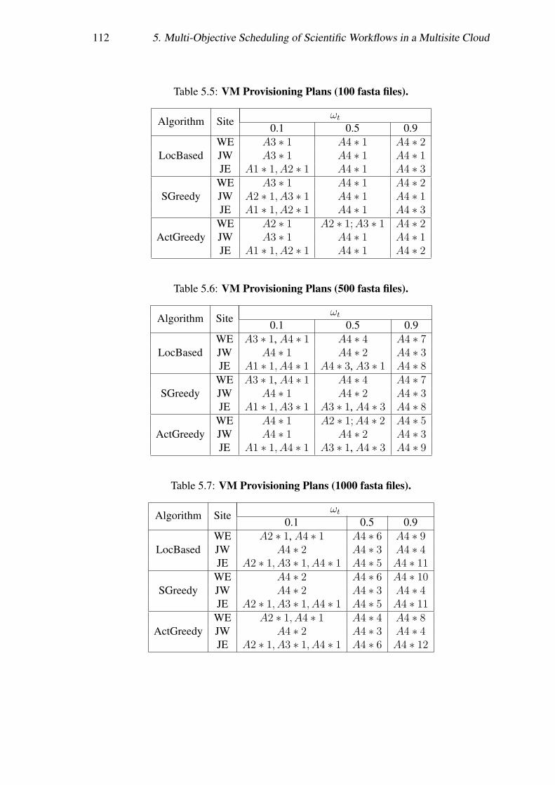
112 5. Multi-Objective Scheduling of Scientific Workflows in a Multisite Cloud
Table 5.5: VM Provisioning Plans (100 fasta files).
Algorithm Siteωt
0.1 0.5 0.9
LocBasedWE A3 ∗ 1 A4 ∗ 1 A4 ∗ 2JW A3 ∗ 1 A4 ∗ 1 A4 ∗ 1JE A1 ∗ 1, A2 ∗ 1 A4 ∗ 1 A4 ∗ 3
SGreedyWE A3 ∗ 1 A4 ∗ 1 A4 ∗ 2JW A2 ∗ 1, A3 ∗ 1 A4 ∗ 1 A4 ∗ 1JE A1 ∗ 1, A2 ∗ 1 A4 ∗ 1 A4 ∗ 3
ActGreedyWE A2 ∗ 1 A2 ∗ 1;A3 ∗ 1 A4 ∗ 2JW A3 ∗ 1 A4 ∗ 1 A4 ∗ 1JE A1 ∗ 1, A2 ∗ 1 A4 ∗ 1 A4 ∗ 2
Table 5.6: VM Provisioning Plans (500 fasta files).
Algorithm Siteωt
0.1 0.5 0.9
LocBasedWE A3 ∗ 1, A4 ∗ 1 A4 ∗ 4 A4 ∗ 7JW A4 ∗ 1 A4 ∗ 2 A4 ∗ 3JE A1 ∗ 1, A4 ∗ 1 A4 ∗ 3, A3 ∗ 1 A4 ∗ 8
SGreedyWE A3 ∗ 1, A4 ∗ 1 A4 ∗ 4 A4 ∗ 7JW A4 ∗ 1 A4 ∗ 2 A4 ∗ 3JE A1 ∗ 1, A3 ∗ 1 A3 ∗ 1, A4 ∗ 3 A4 ∗ 8
ActGreedyWE A4 ∗ 1 A2 ∗ 1;A4 ∗ 2 A4 ∗ 5JW A4 ∗ 1 A4 ∗ 2 A4 ∗ 3JE A1 ∗ 1, A4 ∗ 1 A3 ∗ 1, A4 ∗ 3 A4 ∗ 9
Table 5.7: VM Provisioning Plans (1000 fasta files).
Algorithm Siteωt
0.1 0.5 0.9
LocBasedWE A2 ∗ 1, A4 ∗ 1 A4 ∗ 6 A4 ∗ 9JW A4 ∗ 2 A4 ∗ 3 A4 ∗ 4JE A2 ∗ 1, A3 ∗ 1, A4 ∗ 1 A4 ∗ 5 A4 ∗ 11
SGreedyWE A4 ∗ 2 A4 ∗ 6 A4 ∗ 10JW A4 ∗ 2 A4 ∗ 3 A4 ∗ 4JE A2 ∗ 1, A3 ∗ 1, A4 ∗ 1 A4 ∗ 5 A4 ∗ 11
ActGreedyWE A2 ∗ 1, A4 ∗ 1 A4 ∗ 4 A4 ∗ 8JW A4 ∗ 2 A4 ∗ 3 A4 ∗ 4JE A2 ∗ 1, A3 ∗ 1, A4 ∗ 1 A4 ∗ 6 A4 ∗ 12
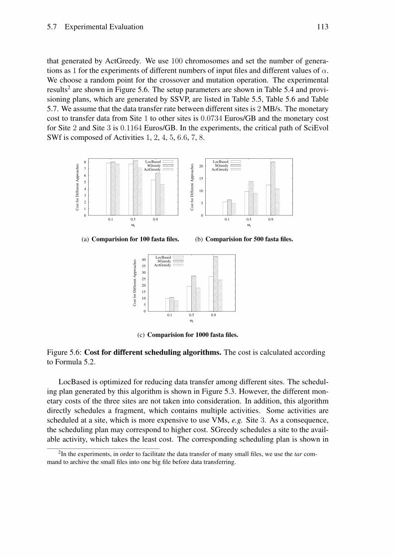
5.7 Experimental Evaluation 113
that generated by ActGreedy. We use 100 chromosomes and set the number of genera-tions as 1 for the experiments of different numbers of input files and different values of α.We choose a random point for the crossover and mutation operation. The experimentalresults2 are shown in Figure 5.6. The setup parameters are shown in Table 5.4 and provi-sioning plans, which are generated by SSVP, are listed in Table 5.5, Table 5.6 and Table5.7. We assume that the data transfer rate between different sites is 2 MB/s. The monetarycost to transfer data from Site 1 to other sites is 0.0734 Euros/GB and the monetary costfor Site 2 and Site 3 is 0.1164 Euros/GB. In the experiments, the critical path of SciEvolSWf is composed of Activities 1, 2, 4, 5, 6.6, 7, 8.
0
1
2
3
4
5
6
7
8
0.1 0.5 0.9
Cost
for D
iffer
ent A
ppro
ache
s
ωt
LocBasedSGreedy
ActGreedy
(a) Comparision for 100 fasta files.
0
5
10
15
20
0.1 0.5 0.9
Cost
for D
iffer
ent A
ppro
ache
s
ωt
LocBasedSGreedy
ActGreedy
(b) Comparision for 500 fasta files.
0
5
10
15
20
25
30
35
40
0.1 0.5 0.9
Cost
for D
iffer
ent A
ppro
ache
s
ωt
LocBasedSGreedy
ActGreedy
(c) Comparision for 1000 fasta files.
Figure 5.6: Cost for different scheduling algorithms. The cost is calculated accordingto Formula 5.2.
LocBased is optimized for reducing data transfer among different sites. The schedul-ing plan generated by this algorithm is shown in Figure 5.3. However, the different mon-etary costs of the three sites are not taken into consideration. In addition, this algorithmdirectly schedules a fragment, which contains multiple activities. Some activities arescheduled at a site, which is more expensive to use VMs, e.g. Site 3. As a consequence,the scheduling plan may correspond to higher cost. SGreedy schedules a site to the avail-able activity, which takes the least cost. The corresponding scheduling plan is shown in
2In the experiments, in order to facilitate the data transfer of many small files, we use the tar com-mand to archive the small files into one big file before data transferring.
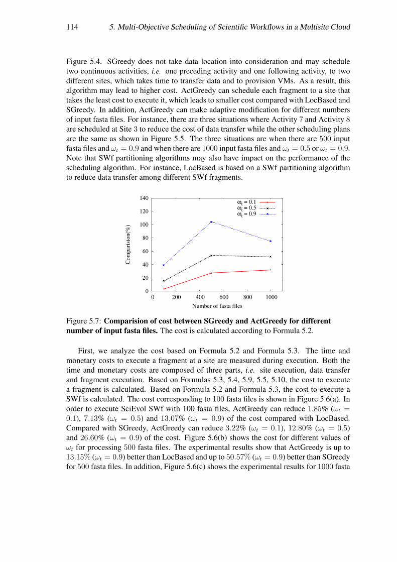
114 5. Multi-Objective Scheduling of Scientific Workflows in a Multisite Cloud
Figure 5.4. SGreedy does not take data location into consideration and may scheduletwo continuous activities, i.e. one preceding activity and one following activity, to twodifferent sites, which takes time to transfer data and to provision VMs. As a result, thisalgorithm may lead to higher cost. ActGreedy can schedule each fragment to a site thattakes the least cost to execute it, which leads to smaller cost compared with LocBased andSGreedy. In addition, ActGreedy can make adaptive modification for different numbersof input fasta files. For instance, there are three situations where Activity 7 and Activity 8are scheduled at Site 3 to reduce the cost of data transfer while the other scheduling plansare the same as shown in Figure 5.5. The three situations are when there are 500 inputfasta files and ωt = 0.9 and when there are 1000 input fasta files and ωt = 0.5 or ωt = 0.9.Note that SWf partitioning algorithms may also have impact on the performance of thescheduling algorithm. For instance, LocBased is based on a SWf partitioning algorithmto reduce data transfer among different SWf fragments.
0
20
40
60
80
100
120
140
0 200 400 600 800 1000
Com
paris
ion(
%)
Number of fasta files
ωt = 0.1ωt = 0.5ωt = 0.9
Figure 5.7: Comparision of cost between SGreedy and ActGreedy for differentnumber of input fasta files. The cost is calculated according to Formula 5.2.
First, we analyze the cost based on Formula 5.2 and Formula 5.3. The time andmonetary costs to execute a fragment at a site are measured during execution. Both thetime and monetary costs are composed of three parts, i.e. site execution, data transferand fragment execution. Based on Formulas 5.3, 5.4, 5.9, 5.5, 5.10, the cost to executea fragment is calculated. Based on Formula 5.2 and Formula 5.3, the cost to execute aSWf is calculated. The cost corresponding to 100 fasta files is shown in Figure 5.6(a). Inorder to execute SciEvol SWf with 100 fasta files, ActGreedy can reduce 1.85% (ωt =0.1), 7.13% (ωt = 0.5) and 13.07% (ωt = 0.9) of the cost compared with LocBased.Compared with SGreedy, ActGreedy can reduce 3.22% (ωt = 0.1), 12.80% (ωt = 0.5)and 26.60% (ωt = 0.9) of the cost. Figure 5.6(b) shows the cost for different values ofωt for processing 500 fasta files. The experimental results show that ActGreedy is up to13.15% (ωt = 0.9) better than LocBased and up to 50.57% (ωt = 0.9) better than SGreedyfor 500 fasta files. In addition, Figure 5.6(c) shows the experimental results for 1000 fasta
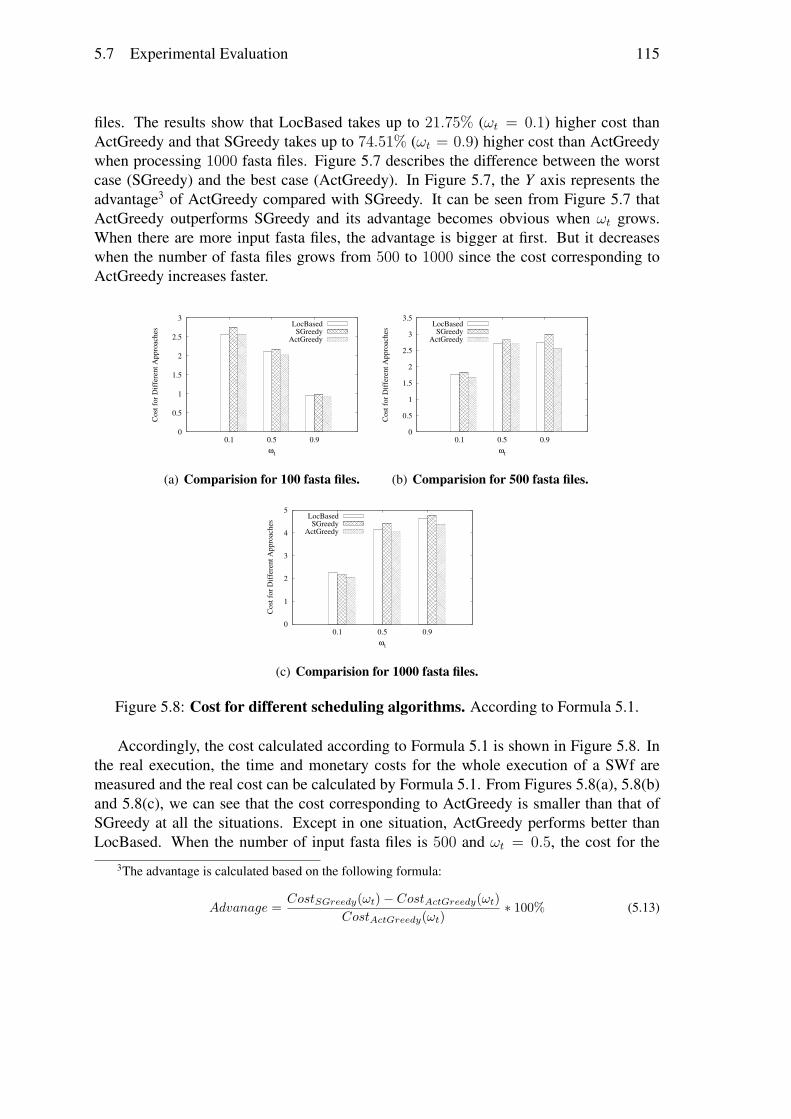
5.7 Experimental Evaluation 115
files. The results show that LocBased takes up to 21.75% (ωt = 0.1) higher cost thanActGreedy and that SGreedy takes up to 74.51% (ωt = 0.9) higher cost than ActGreedywhen processing 1000 fasta files. Figure 5.7 describes the difference between the worstcase (SGreedy) and the best case (ActGreedy). In Figure 5.7, the Y axis represents theadvantage3 of ActGreedy compared with SGreedy. It can be seen from Figure 5.7 thatActGreedy outperforms SGreedy and its advantage becomes obvious when ωt grows.When there are more input fasta files, the advantage is bigger at first. But it decreaseswhen the number of fasta files grows from 500 to 1000 since the cost corresponding toActGreedy increases faster.
0
0.5
1
1.5
2
2.5
3
0.1 0.5 0.9
Cost
for D
iffer
ent A
ppro
ache
s
ωt
LocBasedSGreedy
ActGreedy
(a) Comparision for 100 fasta files.
0
0.5
1
1.5
2
2.5
3
3.5
0.1 0.5 0.9
Cost
for D
iffer
ent A
ppro
ache
s
ωt
LocBasedSGreedy
ActGreedy
(b) Comparision for 500 fasta files.
0
1
2
3
4
5
0.1 0.5 0.9
Cost
for D
iffer
ent A
ppro
ache
s
ωt
LocBasedSGreedy
ActGreedy
(c) Comparision for 1000 fasta files.
Figure 5.8: Cost for different scheduling algorithms. According to Formula 5.1.
Accordingly, the cost calculated according to Formula 5.1 is shown in Figure 5.8. Inthe real execution, the time and monetary costs for the whole execution of a SWf aremeasured and the real cost can be calculated by Formula 5.1. From Figures 5.8(a), 5.8(b)and 5.8(c), we can see that the cost corresponding to ActGreedy is smaller than that ofSGreedy at all the situations. Except in one situation, ActGreedy performs better thanLocBased. When the number of input fasta files is 500 and ωt = 0.5, the cost for the
3The advantage is calculated based on the following formula:
Advanage = CostSGreedy(ωt)− CostActGreedy(ωt)CostActGreedy(ωt)
∗ 100% (5.13)
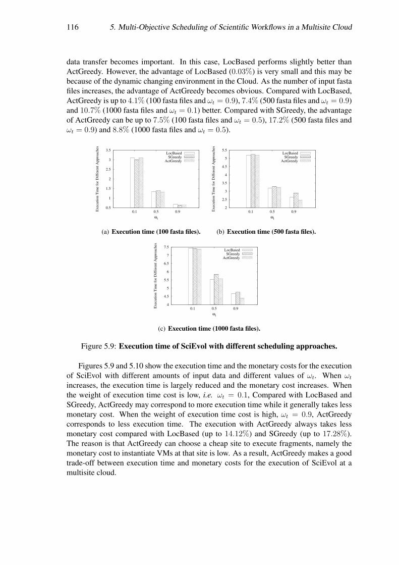
116 5. Multi-Objective Scheduling of Scientific Workflows in a Multisite Cloud
data transfer becomes important. In this case, LocBased performs slightly better thanActGreedy. However, the advantage of LocBased (0.03%) is very small and this may bebecause of the dynamic changing environment in the Cloud. As the number of input fastafiles increases, the advantage of ActGreedy becomes obvious. Compared with LocBased,ActGreedy is up to 4.1% (100 fasta files and ωt = 0.9), 7.4% (500 fasta files and ωt = 0.9)and 10.7% (1000 fasta files and ωt = 0.1) better. Compared with SGreedy, the advantageof ActGreedy can be up to 7.5% (100 fasta files and ωt = 0.5), 17.2% (500 fasta files andωt = 0.9) and 8.8% (1000 fasta files and ωt = 0.5).
0.5
1
1.5
2
2.5
3
3.5
0.1 0.5 0.9Exec
utio
n Ti
me
for D
iffer
ent A
ppro
ache
s
ωt
LocBasedSGreedy
ActGreedy
(a) Execution time (100 fasta files).
2
2.5
3
3.5
4
4.5
5
5.5
0.1 0.5 0.9Exec
utio
n Ti
me
for D
iffer
ent A
ppro
ache
sωt
LocBasedSGreedy
ActGreedy
(b) Execution time (500 fasta files).
4
4.5
5
5.5
6
6.5
7
7.5
0.1 0.5 0.9Exec
utio
n Ti
me
for D
iffer
ent A
ppro
ache
s
ωt
LocBasedSGreedy
ActGreedy
(c) Execution time (1000 fasta files).
Figure 5.9: Execution time of SciEvol with different scheduling approaches.
Figures 5.9 and 5.10 show the execution time and the monetary costs for the executionof SciEvol with different amounts of input data and different values of ωt. When ωtincreases, the execution time is largely reduced and the monetary cost increases. Whenthe weight of execution time cost is low, i.e. ωt = 0.1, Compared with LocBased andSGreedy, ActGreedy may correspond to more execution time while it generally takes lessmonetary cost. When the weight of execution time cost is high, ωt = 0.9, ActGreedycorresponds to less execution time. The execution with ActGreedy always takes lessmonetary cost compared with LocBased (up to 14.12%) and SGreedy (up to 17.28%).The reason is that ActGreedy can choose a cheap site to execute fragments, namely themonetary cost to instantiate VMs at that site is low. As a result, ActGreedy makes a goodtrade-off between execution time and monetary costs for the execution of SciEvol at amultisite cloud.
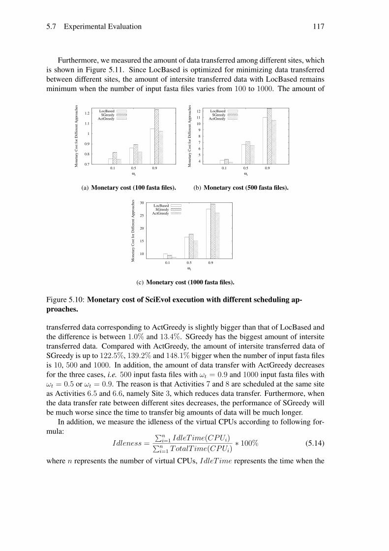
5.7 Experimental Evaluation 117
Furthermore, we measured the amount of data transferred among different sites, whichis shown in Figure 5.11. Since LocBased is optimized for minimizing data transferredbetween different sites, the amount of intersite transferred data with LocBased remainsminimum when the number of input fasta files varies from 100 to 1000. The amount of
0.7
0.8
0.9
1
1.1
1.2
0.1 0.5 0.9Mon
etar
y Co
st fo
r Diff
eren
t App
roac
hes
ωt
LocBasedSGreedy
ActGreedy
(a) Monetary cost (100 fasta files).
456789
101112
0.1 0.5 0.9Mon
etar
y Co
st fo
r Diff
eren
t App
roac
hes
ωt
LocBasedSGreedy
ActGreedy
(b) Monetary cost (500 fasta files).
10
15
20
25
30
0.1 0.5 0.9Mon
etar
y Co
st fo
r Diff
eren
t App
roac
hes
ωt
LocBasedSGreedy
ActGreedy
(c) Monetary cost (1000 fasta files).
Figure 5.10: Monetary cost of SciEvol execution with different scheduling ap-proaches.
transferred data corresponding to ActGreedy is slightly bigger than that of LocBased andthe difference is between 1.0% and 13.4%. SGreedy has the biggest amount of intersitetransferred data. Compared with ActGreedy, the amount of intersite transferred data ofSGreedy is up to 122.5%, 139.2% and 148.1% bigger when the number of input fasta filesis 10, 500 and 1000. In addition, the amount of data transfer with ActGreedy decreasesfor the three cases, i.e. 500 input fasta files with ωt = 0.9 and 1000 input fasta files withωt = 0.5 or ωt = 0.9. The reason is that Activities 7 and 8 are scheduled at the same siteas Activities 6.5 and 6.6, namely Site 3, which reduces data transfer. Furthermore, whenthe data transfer rate between different sites decreases, the performance of SGreedy willbe much worse since the time to transfer big amounts of data will be much longer.
In addition, we measure the idleness of the virtual CPUs according to following for-mula:
Idleness =∑ni=1 IdleT ime(CPUi)∑ni=1 TotalT ime(CPUi)
∗ 100% (5.14)
where n represents the number of virtual CPUs, IdleT ime represents the time when the
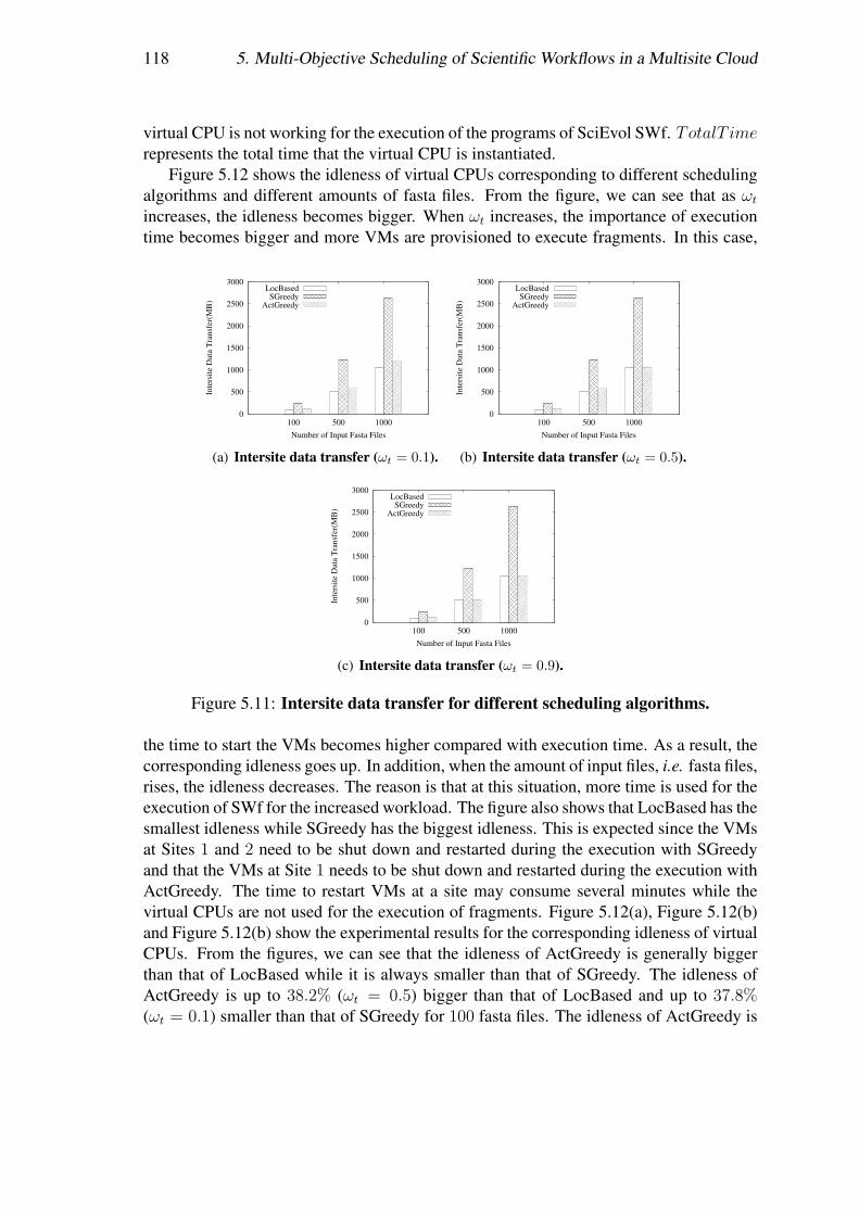
118 5. Multi-Objective Scheduling of Scientific Workflows in a Multisite Cloud
virtual CPU is not working for the execution of the programs of SciEvol SWf. TotalT imerepresents the total time that the virtual CPU is instantiated.
Figure 5.12 shows the idleness of virtual CPUs corresponding to different schedulingalgorithms and different amounts of fasta files. From the figure, we can see that as ωtincreases, the idleness becomes bigger. When ωt increases, the importance of executiontime becomes bigger and more VMs are provisioned to execute fragments. In this case,
0
500
1000
1500
2000
2500
3000
100 500 1000
Inte
rsite
Dat
a T
rans
fer(
MB
)
Number of Input Fasta Files
LocBasedSGreedy
ActGreedy
(a) Intersite data transfer (ωt = 0.1).
0
500
1000
1500
2000
2500
3000
100 500 1000
Inte
rsite
Dat
a T
rans
fer(
MB
)
Number of Input Fasta Files
LocBasedSGreedy
ActGreedy
(b) Intersite data transfer (ωt = 0.5).
0
500
1000
1500
2000
2500
3000
100 500 1000
Inte
rsite
Dat
a T
rans
fer(
MB
)
Number of Input Fasta Files
LocBasedSGreedy
ActGreedy
(c) Intersite data transfer (ωt = 0.9).
Figure 5.11: Intersite data transfer for different scheduling algorithms.
the time to start the VMs becomes higher compared with execution time. As a result, thecorresponding idleness goes up. In addition, when the amount of input files, i.e. fasta files,rises, the idleness decreases. The reason is that at this situation, more time is used for theexecution of SWf for the increased workload. The figure also shows that LocBased has thesmallest idleness while SGreedy has the biggest idleness. This is expected since the VMsat Sites 1 and 2 need to be shut down and restarted during the execution with SGreedyand that the VMs at Site 1 needs to be shut down and restarted during the execution withActGreedy. The time to restart VMs at a site may consume several minutes while thevirtual CPUs are not used for the execution of fragments. Figure 5.12(a), Figure 5.12(b)and Figure 5.12(b) show the experimental results for the corresponding idleness of virtualCPUs. From the figures, we can see that the idleness of ActGreedy is generally biggerthan that of LocBased while it is always smaller than that of SGreedy. The idleness ofActGreedy is up to 38.2% (ωt = 0.5) bigger than that of LocBased and up to 37.8%(ωt = 0.1) smaller than that of SGreedy for 100 fasta files. The idleness of ActGreedy is
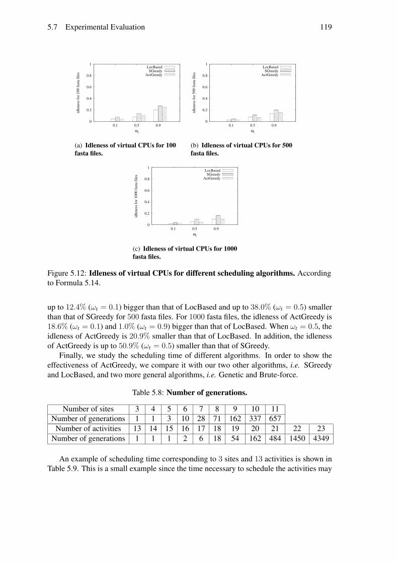
5.7 Experimental Evaluation 119
0
0.2
0.4
0.6
0.8
1
0.1 0.5 0.9
idle
ness
for 1
00 fa
sta
file
s
ωt
LocBasedSGreedy
ActGreedy
(a) Idleness of virtual CPUs for 100fasta files.
0
0.2
0.4
0.6
0.8
1
0.1 0.5 0.9
idle
ness
for 5
00 fa
sta
file
s
ωt
LocBasedSGreedy
ActGreedy
(b) Idleness of virtual CPUs for 500fasta files.
0
0.2
0.4
0.6
0.8
1
0.1 0.5 0.9
idle
ness
for 1
000
fast
a fi
les
ωt
LocBasedSGreedy
ActGreedy
(c) Idleness of virtual CPUs for 1000fasta files.
Figure 5.12: Idleness of virtual CPUs for different scheduling algorithms. Accordingto Formula 5.14.
up to 12.4% (ωt = 0.1) bigger than that of LocBased and up to 38.0% (ωt = 0.5) smallerthan that of SGreedy for 500 fasta files. For 1000 fasta files, the idleness of ActGreedy is18.6% (ωt = 0.1) and 1.0% (ωt = 0.9) bigger than that of LocBased. When ωt = 0.5, theidleness of ActGreedy is 20.9% smaller than that of LocBased. In addition, the idlenessof ActGreedy is up to 50.9% (ωt = 0.5) smaller than that of SGreedy.
Finally, we study the scheduling time of different algorithms. In order to show theeffectiveness of ActGreedy, we compare it with our two other algorithms, i.e. SGreedyand LocBased, and two more general algorithms, i.e. Genetic and Brute-force.
Table 5.8: Number of generations.
Number of sites 3 4 5 6 7 8 9 10 11Number of generations 1 1 3 10 28 71 162 337 657
Number of activities 13 14 15 16 17 18 19 20 21 22 23Number of generations 1 1 1 2 6 18 54 162 484 1450 4349
An example of scheduling time corresponding to 3 sites and 13 activities is shown inTable 5.9. This is a small example since the time necessary to schedule the activities may

120 5. Multi-Objective Scheduling of Scientific Workflows in a Multisite Cloud
Figure 5.13: SciEvol SWf. Activities 9 − n are added control activities, which have noworkload.
be unfeasible for Brute-force and Genetic when the numbers of activities or sites becomehigh. Then, we vary the numbers of activities or sites. When we increase the number ofsites, we fix the number of activities at 13 and when we increase the number of activities,we fix the number of sites to 3. The number of generations for different numbers of activi-ties or different numbers of sites is shown in Table 5.8. Since the search space gets biggerwhen the number of activities or sites increases, we increase the number of generationsin order to evaluate at least 30% of all the possible scheduling plans for Genetic. We addadditional control activities in the SciEvol SWf, which have little workload but increasethe search space of scheduling plans. The modified SciEvol SWf is shown in Figure5.13 and the scheduling time corresponding to different numbers of activities is shown in5.14(a). In addition, we measure the scheduling time corresponding to different numbersof sites while using the original SciEvol SWf, as shown in Figure 5.14(b). The unit ofscheduling time is millisecond. The data constraint remains the same while the numberof input files is 100 and α equals to 0.9. In the experiments, only ActGreedy generatesthe same scheduling plans as that of Brute-force. Since the point of mutation operationand the points of crossover operation of Genetic are randomly selected, the schedulingplans generated by Genetic may not be stable, i.e. the scheduling plans may not be thesame for each execution of the algorithm. Both LocBased and SGreedy cannot generatethe optimal scheduling plans as that of Brute-force.
Table 5.9: Comparison of scheduling algorithms.
Algorithms Scheduling time (ms)LocBased 0.010SGreedy 0.014
ActGreedy 1.260Genetic 727
Brute-force 161
Table 5.9 shows that the scheduling time of Genetic and Brute-force is much longer
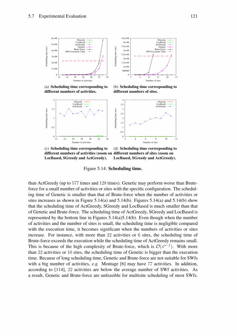
5.7 Experimental Evaluation 121
0
1e+06
2e+06
3e+06
4e+06
5e+06
6e+06
12 14 16 18 20 22 24
Sche
dulin
g tim
e (m
s)
Number of activities
SGreedyLocBased
ActGreedyGenetic
Brute ForceSWf Execution Time
(a) Scheduling time corresponding todifferent numbers of activities.
0
500000
1e+06
1.5e+06
2e+06
2.5e+06
3e+06
3.5e+06
4e+06
4.5e+06
2 4 6 8 10 12
Sche
dulin
g tim
e (m
s)
Number of sites
SGreedyLocBased
ActGreedyGenetic
Brute ForceSWf Execution Time
(b) Scheduling time corresponding todifferent numbers of sites.
0
0.5
1
1.5
2
12 14 16 18 20 22 24
Sche
dulin
g tim
e (m
s)
Number of activities
SGreedyLocBased
ActGreedy
(c) Scheduling time corresponding todifferent numbers of activities (zoom onLocBased, SGreedy and ActGreedy).
0
0.5
1
1.5
2
2.5
3
3.5
4
2 4 6 8 10 12
Sche
dulin
g tim
e (m
s)
Number of sites
SGreedyLocBased
ActGreedy
(d) Scheduling time corresponding todifferent numbers of sites (zoom onLocBased, SGreedy and ActGreedy).
Figure 5.14: Scheduling time.
than ActGreedy (up to 577 times and 128 times). Genetic may perform worse than Brute-force for a small number of activities or sites with the specific configuration. The schedul-ing time of Genetic is smaller than that of Brute-force when the number of activities orsites increases as shown in Figure 5.14(a) and 5.14(b). Figures 5.14(a) and 5.14(b) showthat the scheduling time of ActGreedy, SGreedy and LocBased is much smaller than thatof Genetic and Brute-force. The scheduling time of ActGreedy, SGreedy and LocBased isrepresented by the bottom line in Figures 5.14(a)5.14(b). Even though when the numberof activities and the number of sites is small, the scheduling time is negligible comparedwith the execution time, it becomes significant when the numbers of activities or sitesincrease. For instance, with more than 22 activities or 6 sites, the scheduling time ofBrute-force exceeds the execution while the scheduling time of ActGreedy remains small.This is because of the high complexity of Brute-force, which is O(sn−f ). With morethan 22 activities or 10 sites, the scheduling time of Genetic is bigger than the executiontime. Because of long scheduling time, Genetic and Brute-force are not suitable for SWfswith a big number of activities, e.g. Montage [6] may have 77 activities. In addition,according to [114], 22 activities are below the average number of SWf activities. Asa result, Genetic and Brute-force are unfeasible for multisite scheduling of most SWfs.
122 5. Multi-Objective Scheduling of Scientific Workflows in a Multisite Cloud
These two algorithms are not suitable for SWf scheduling with a big number of sites.For instance, Azure has 15 sites (regions). Although the scheduling time of ActGreedy ismuch bigger (see Figures 5.14(c)5.14(d) for details) than that of SGreedy and LocBased,it remains reasonable compared with the overall SWf execution time.
The experimental results show that although ActGreedy may yield more data trans-ferred among different sites and higher idleness (compared with LocBased), it generallyyields smaller cost compared with both LocBased and SGreedy and the scheduling timeof ActGreedy is much lower than that of Genetic and Brute-force.
5.8 ConclusionScientists usually make intensive usage of parallelism techniques in HPC environments.However, it is not simple to schedule and manage executions of SWfs, particularly inmultisite cloud environments, which present different characteristics in comparison witha single site cloud. To increase the uptake of the cloud model for executing SWfs thatdemand HPC capabilities provided by a multisite cloud and to benefit from data locality,new solutions have to be developed, especially for scheduling SWf fragments in cloudresources. In previous work [52] we have addressed SWf execution in a single site cloudusing a scheduling algorithm but these solutions are not suitable for a multisite cloud.
In this chapter, we proposed a new multi-objective scheduling approach, i.e. Act-Greedy, for SWfs in a multisite cloud (from the same provider). We first proposed a novelmulti-objective cost model, which aims at minimizing two costs: execution time and mon-etary costs. Our proposed fragment scheduling approach that is ActGreedy, allows forconsidering stored data constraints while reducing the cost based on the multi-objectivecost model to execute a SWf in a multisite cloud. We used a real SWf that is SciEvol,with real data from the bioinformatics domain as a use case. We evaluated our approachesby executing SciEvol in Microsoft Azure cloud. The results show that since ActGreedymakes a good trade-off between execution time and monetary costs, ActGreedy leadsto the least total normalized cost, which is calculated based on the multi-objective costmodel, than LocBased (up to 10.7%) and SGreedy (up to 17.2%) approaches. In addition,compared with LocBased (up to 14.12%) and SGreedy (up to 17.28%), ActGreedy alwayscorresponds to less monetary cost since it can choose cheap cloud sites to execute SWffragments. Furthermore, compared with SGreedy, ActGreedy corresponds to more thantwo times smaller amounts of transferred data. Additionally, ActGreedy scales very well,i.e. it takes a very small time to generate the optimal or near optimal scheduling planswhen the number of activities or sites increases, compared with general approaches, e.g.Genetic and Brute-force.

Chapter 6
Task Scheduling with ProvenanceSupport in Multisite Clouds
Recently, some Scientific Workflow Management Systems (SWfMSs) with provenancesupport (e.g. Chiron) have been deployed in the cloud. However, they typically use asingle cloud site. In this chapter, we consider a multisite cloud, where the data and com-puting resources are distributed at different sites (possibly in different regions). Based ona multisite architecture of SWfMS, i.e. multisite Chiron, and its provenance model, wepropose a multisite task scheduling algorithm that considers the time to generate prove-nance data. This thesis is based on [121].
Section 6.3 presents the problems for task scheduling of SWf execution in a multisitecloud environment. Then, Section 6.4 gives the design of a multisite SWfMS. Afterwards,Section 6.5 explains our proposed scheduling algorithm. Section 6.6 gives our our exten-sive experimental evaluation of the algorithm using Microsoft Azure multisite cloud andtwo real-life scientific workflows (Buzz and Montage). The results show that our schedul-ing algorithm is much better than baseline algorithms in terms of execution time and theamounts of intersite transferred data.
6.1 Proposal Overview and MotivationsSWfs are generally used to model the data processing of large scale in silico scientificexperiments as a graph, in which vertices represent data processing activities and edgesrepresent dependencies between them. Since SWf activities may process multiple datachunks, one activity can correspond to several executable tasks for different parts of inputdata during SWf execution. Thus, efficiently executing data-intensive SWfs, e.g. Montage[6] and Buzz [64], becomes an important issue.
Some implementations of SWfMSs are publicly available, e.g. Pegasus [60] and Ch-iron [139]. A SWfMS generally supports provenance data, which is the metadata thatcaptures the derivation history of a dataset [120], during SWf execution. Provenancedata, which is used for SWf analysis and SWf reproducibility, may be as important as the
123

124 6. Task Scheduling with Provenance Support in Multisite Clouds
scientifc experiment itself [120]. The provenance data is typically stored in a databaseto provide on-line provenance query [129], and contains the information regarding activ-ities, tasks and files. During the execution of a task, there may be multiple exchanges ofprovenance data between the computing node and the provenance database.
Recently, some SWfMSs with provenance support (e.g. Chiron) have been deployedin the cloud. However, they typically focus the execution of a SWf at a single cloud siteor in even a single computing node [92][93]. Although there are some multisite solutions[65][150], they do not support provenance data, which is important for the analysis of SWfexecution. However, the data and computing resources (including programs) necessaryto run a SWf may well be distributed at different sites (possibly in different regions), e.g.because of collaboration between different groups of scientists. And it may not be alwayspossible to move all the resources to a single site for execution. Chapter 5 focuses onthe scheduling of fragments, which is coarse-grained and cannot address the problem ofexecuting an activities at multiple sites. In this chapter, we consider a multisite cloud thatis composed of several sites (or data centers) of the same cloud provider, each with itsown resources and data for the execution of each activity. In addition, we also take intoconsideration of the influence of the functionality of provenance data on the SWf multisiteexecution.
To enable SWf execution in a multisite cloud with distributed input data, the executionof the tasks of each activity should be scheduled to a corresponding cloud site (or site forshort). Then, the scheduling problem is to decide at which sites to execute the tasks inorder to achieve a given objective, e.g. reducing execution time. Compared with theapproach of scheduling activities at a single site [122], the task scheduling is fine-grained,which enables the execution of the same activity at different sites to deal with distributeddata and programs. Furthermore, since it may take much time to transfer data between twodifferent sites, the multisite scheduling problem should take into account the resources atdifferent sites, e.g. different bandwidths.
We focus on the task scheduling problem to reduce the makespan, i.e. the executiontime, of executing a SWf in a multisite cloud. We use a distributed SWfMS architecturewith a master site that coordinates the execution of each site and that stores all the prove-nance data of SWf execution. In this architecture, the intersite transferred data can beintermediate data or provenance data produced by SWf execution. The intermediate datais the data generated by executing activities and can also be the input data for the tasks offollowing activities. In the multisite cloud, the bandwidth between two different sites (ofdifferent regions) may be small. For data-intensive SWfs, there may be many data, e.g.intermediate data and provenance data, to transfer across different sites for the executionof a task while the time to execute the task can be very small, e.g. a few seconds or evenless than one second. As a result, the time to transfer intermediate data and the time togenerate the provenance data connot be ignored in the scheduling process. Thus, we alsoconsider the time to transfer both the intermediate data and the provenance data in thescheduling process in order to better reduce the overall execution time of SWf execution.
We make the following contributions. First, we propose multisite Chiron, with anovel architecture to execute SWfs in a multisite cloud environment while generating
6.2 Related Work 125
provenance data. Second, an extended multisite provenance model and global prove-nance management of distributed provenance data in multisite cloud. Third, we proposea novel multisite task scheduling algorithm, i.e. Data-Intensive Multisite task scheduling(DIM), for SWf execution with provenance support in multisite Chiron. Fourth, we makean extensive experimental evaluation, based on the implementation of multisite Chiron inMicrosoft Azure, and using two real SWf use cases (Buzz and Montage).
6.2 Related WorkClassic scheduling algorithms, e.g. Opportunistic Load Balancing (OLB) [125], Mini-mum Completion Time (MCT) [125], min-min [67], max-min [67] and HeterogeneousEarliest Finish Time (HEFT) [186], address the scheduling problem for the objective ofreducing execution time within a single site. The OLB algorithm randomly assigns eachtask to an available computing node without considering the feature of the task or thecomputing node. The MCT algorithm schedules each task to the computing node that canfinish the execution first. HEFT gives the priority to each task according to the dependen-cies of tasks and the workload of the task. Then, it schedules the tasks with the highestpriority to the computing node that can finish the execution first. The min-min algorithmschedules the task, which takes the least time to execute, to the computing node that canfinish the execution first. The max-min algorithm schedules the task, which takes thebiggest time to execute, to the computing node that can finish the execution first. For thetasks of the same activity, they are independent of each other and have the same estimatedexecution time. As a result, the HEFT, min-min and max-min algorithms degrade to theMCT algorithm for this kind of tasks. Some other solutions [168][177][196] for SWfscheduling also focus on single site execution. These techniques do not consider the timeto generate provenance data. Dean and Ghemawat [55] propose to schedule tasks to wherethe data is. Although this method focuses on single site, it considers the cost to transferdata among different computing nodes. However, this algorithm depends on the locationof data. When the data is not evenly distributed at each computing node, this algorithmmay lead to unbalanced load at some computing nodes and long execution time of tasks.De Oliveira et al. [52] propose a provenance based task scheduling algorithm for singlesite cloud environments. Some adaptation of SWfMSs [28][34] in the cloud environmentcan provide the parallelism in workflow level or activity level, which is coarse-grained,at a single site cloud. These methods cannot perform parallelism of the tasks of the sameactivities and they cannot handle the distributed input data at different sites.
Duan et al. [65] propose a multisite multi-objective scheduling algorithm with consid-eration of different bandwidths in a multisite environment. However, they do not considerthe input data distribution at different sites and do not provide provenance support, , whichmay incur much time for intersite provenance data transfer. In Chapter 5, we proposed asolution of multisite activity scheduling of SWfs according to the data location. However,the activity scheduling method is coarse-grained: it can schedule the execution of each ac-tivity to a site but cannot schedule different tasks of one activity to different sites. Thus, it

126 6. Task Scheduling with Provenance Support in Multisite Clouds
Figure 6.1: Activity and tasks.
cannot handle the distributed input data of a SWf in a multisite cloud environment. Luis etal. [150] propose caching metadata in the memory and replicating the metadata for SWfexecution in a multisite cloud. The metadata is the description information of files at eachsite. In this method, data transfer is analyzed in multi-site SWf execution, stressing theimportance of optimizing data provisioning. However, the metadata is not yet explored ontask scheduling and, they just simulated SWf execution in the experiments. Their methodcan be used to optimize the metadata management in our multisite Chiron in the future.Hadoop [185] is extended to multiple sites while the the existing approaches do not con-sider the provenance support or different bandwidths among different sites for the taskscheduling [184].
6.3 Problem DefinitionThis section introduces some important terms, i.e. SWf and multisite cloud, and formallydefines the task scheduling problem we address.
A SWf can be described as a Directed Acyclic Graph (DAG) denoted by W (V ,E).Let V = {v1, v2, ..., vn} be a set of vertices, which represent the scientific data processingactivities. E = {ei,j: vi, vj ∈ V and Activity vj consumes the output data of Activityvi } represents a set of edges that correspond to dependencies between activities in V .Activity vi is the parent activity of Activity vj and Activity vj is the child activity ofActivity vi. If it has no parent activity, an activity is a start activity. If it has no childactivity, an activity is an end activity. If it has neither parent activity nor child activity,an activity is an intermediate activity. Since an activity may process big amount of data,it corresponds to multiple tasks. Thus, as shown in Figure 6.1, an activity Ak may haven tasks {t1, t2, ..., tn}, each consuming a data chunk produced by the tasks of parentactivities of Activity Ak, i.e. Activities Ai and Aj . A data-intensive SWf is the SWf thatit is difficult to manage or transfer data compared to the data processing. For instance,for data-intensive SWfs, the time to transfer data cannot be ignored compared with the
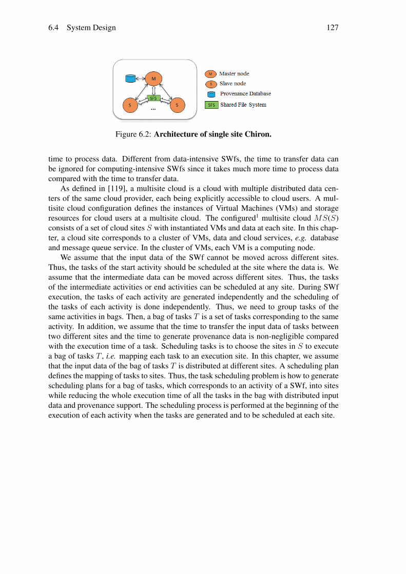
6.4 System Design 127
Figure 6.2: Architecture of single site Chiron.
time to process data. Different from data-intensive SWfs, the time to transfer data canbe ignored for computing-intensive SWfs since it takes much more time to process datacompared with the time to transfer data.
As defined in [119], a multisite cloud is a cloud with multiple distributed data cen-ters of the same cloud provider, each being explicitly accessible to cloud users. A mul-tisite cloud configuration defines the instances of Virtual Machines (VMs) and storageresources for cloud users at a multisite cloud. The configured1 multisite cloud MS(S)consists of a set of cloud sites S with instantiated VMs and data at each site. In this chap-ter, a cloud site corresponds to a cluster of VMs, data and cloud services, e.g. databaseand message queue service. In the cluster of VMs, each VM is a computing node.
We assume that the input data of the SWf cannot be moved across different sites.Thus, the tasks of the start activity should be scheduled at the site where the data is. Weassume that the intermediate data can be moved across different sites. Thus, the tasksof the intermediate activities or end activities can be scheduled at any site. During SWfexecution, the tasks of each activity are generated independently and the scheduling ofthe tasks of each activity is done independently. Thus, we need to group tasks of thesame activities in bags. Then, a bag of tasks T is a set of tasks corresponding to the sameactivity. In addition, we assume that the time to transfer the input data of tasks betweentwo different sites and the time to generate provenance data is non-negligible comparedwith the execution time of a task. Scheduling tasks is to choose the sites in S to executea bag of tasks T , i.e. mapping each task to an execution site. In this chapter, we assumethat the input data of the bag of tasks T is distributed at different sites. A scheduling plandefines the mapping of tasks to sites. Thus, the task scheduling problem is how to generatescheduling plans for a bag of tasks, which corresponds to an activity of a SWf, into siteswhile reducing the whole execution time of all the tasks in the bag with distributed inputdata and provenance support. The scheduling process is performed at the beginning of theexecution of each activity when the tasks are generated and to be scheduled at each site.
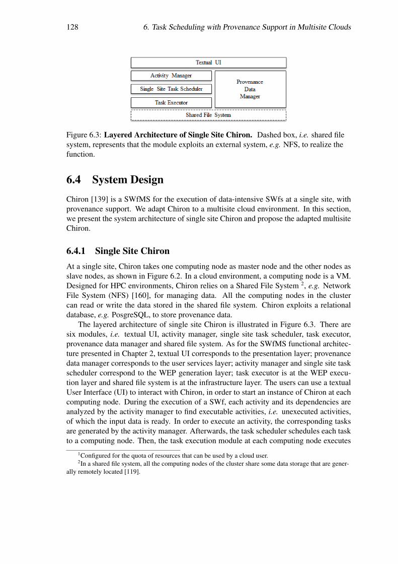
128 6. Task Scheduling with Provenance Support in Multisite Clouds
Figure 6.3: Layered Architecture of Single Site Chiron. Dashed box, i.e. shared filesystem, represents that the module exploits an external system, e.g. NFS, to realize thefunction.
6.4 System DesignChiron [139] is a SWfMS for the execution of data-intensive SWfs at a single site, withprovenance support. We adapt Chiron to a multisite cloud environment. In this section,we present the system architecture of single site Chiron and propose the adapted multisiteChiron.
6.4.1 Single Site ChironAt a single site, Chiron takes one computing node as master node and the other nodes asslave nodes, as shown in Figure 6.2. In a cloud environment, a computing node is a VM.Designed for HPC environments, Chiron relies on a Shared File System 2, e.g. NetworkFile System (NFS) [160], for managing data. All the computing nodes in the clustercan read or write the data stored in the shared file system. Chiron exploits a relationaldatabase, e.g. PosgreSQL, to store provenance data.
The layered architecture of single site Chiron is illustrated in Figure 6.3. There aresix modules, i.e. textual UI, activity manager, single site task scheduler, task executor,provenance data manager and shared file system. As for the SWfMS functional architec-ture presented in Chapter 2, textual UI corresponds to the presentation layer; provenancedata manager corresponds to the user services layer; activity manager and single site taskscheduler correspond to the WEP generation layer; task executor is at the WEP execu-tion layer and shared file system is at the infrastructure layer. The users can use a textualUser Interface (UI) to interact with Chiron, in order to start an instance of Chiron at eachcomputing node. During the execution of a SWf, each activity and its dependencies areanalyzed by the activity manager to find executable activities, i.e. unexecuted activities,of which the input data is ready. In order to execute an activity, the corresponding tasksare generated by the activity manager. Afterwards, the task scheduler schedules each taskto a computing node. Then, the task execution module at each computing node executes
1Configured for the quota of resources that can be used by a cloud user.2In a shared file system, all the computing nodes of the cluster share some data storage that are gener-
ally remotely located [119].

6.4 System Design 129
Figure 6.4: Single Site Provenance Model [139].
the corresponding scheduled tasks. When all the tasks of the executable activity are ex-ecuted, the activity manager analyzes the activities to find new executable activities toexecute. The process of activity analysis, task scheduling and task execution are repeateduntil all activities have been executed. Since the input data, intermediate data and out-put data of SWfs are stored in a shared file system, Chiron does not need to manage datatransfer between different computing nodes. During SWf execution, the activity manager,the task scheduler and the task executor generate provenance data, which is gathered bythe provenance data manager. The provenance data manager is located at the master nodeof the cluster.
The single site provenance model [139] is shown in Figure 6.4. In this model, a SWf iscomposed of several activities. An activity has an operator, i.e. the program for this activ-ity. The status of the activity can be ready, running or finished. The activationCommandof an activity is to execute the activity. The extractorCommand is to generate prove-nance data for the corresponding tasks. The time at which the activity execution starts isexecutionStart and the time at which it ends is executionEnd. One activity is relatedto several tasks, input relations and output relations. One relation is the input or outputparameters for the activity. Each relation has its own attributes and tuples. The tasks ofan activity are generated based on the input relation of the activity. A task processes thefiles associated with the corresponding activity. Each task has a status, i.e. ready, run-ning or finished. In addition, the start time and end time of its execution is recorded asExecutionStart and ExecutionEnd. During execution, the corresponding informationof activities, files and tasks are stored as provenance data.
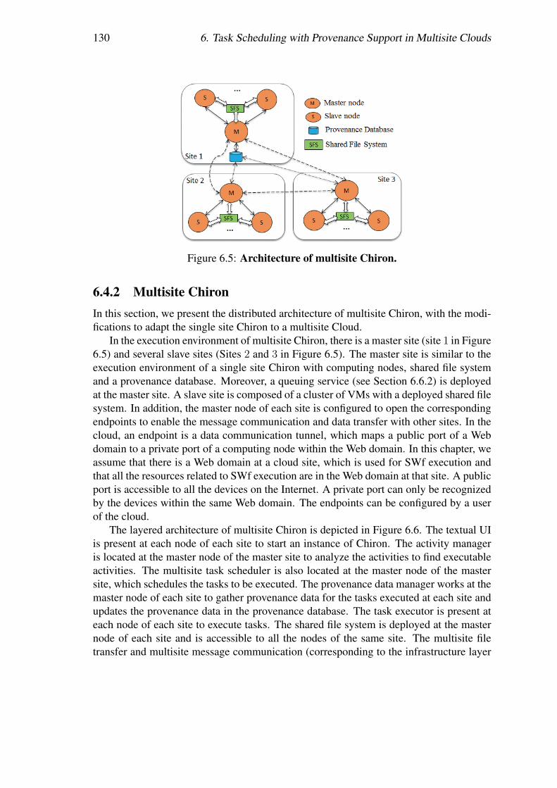
130 6. Task Scheduling with Provenance Support in Multisite Clouds
Figure 6.5: Architecture of multisite Chiron.
6.4.2 Multisite ChironIn this section, we present the distributed architecture of multisite Chiron, with the modi-fications to adapt the single site Chiron to a multisite Cloud.
In the execution environment of multisite Chiron, there is a master site (site 1 in Figure6.5) and several slave sites (Sites 2 and 3 in Figure 6.5). The master site is similar to theexecution environment of a single site Chiron with computing nodes, shared file systemand a provenance database. Moreover, a queuing service (see Section 6.6.2) is deployedat the master site. A slave site is composed of a cluster of VMs with a deployed shared filesystem. In addition, the master node of each site is configured to open the correspondingendpoints to enable the message communication and data transfer with other sites. In thecloud, an endpoint is a data communication tunnel, which maps a public port of a Webdomain to a private port of a computing node within the Web domain. In this chapter, weassume that there is a Web domain at a cloud site, which is used for SWf execution andthat all the resources related to SWf execution are in the Web domain at that site. A publicport is accessible to all the devices on the Internet. A private port can only be recognizedby the devices within the same Web domain. The endpoints can be configured by a userof the cloud.
The layered architecture of multisite Chiron is depicted in Figure 6.6. The textual UIis present at each node of each site to start an instance of Chiron. The activity manageris located at the master node of the master site to analyze the activities to find executableactivities. The multisite task scheduler is also located at the master node of the mastersite, which schedules the tasks to be executed. The provenance data manager works at themaster node of each site to gather provenance data for the tasks executed at each site andupdates the provenance data in the provenance database. The task executor is present ateach node of each site to execute tasks. The shared file system is deployed at the masternode of each site and is accessible to all the nodes of the same site. The multisite filetransfer and multisite message communication (corresponding to the infrastructure layer
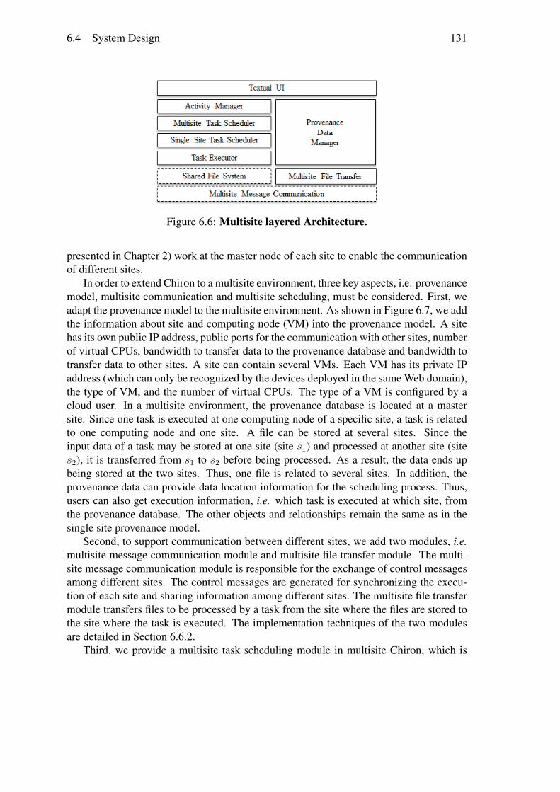
6.4 System Design 131
Figure 6.6: Multisite layered Architecture.
presented in Chapter 2) work at the master node of each site to enable the communicationof different sites.
In order to extend Chiron to a multisite environment, three key aspects, i.e. provenancemodel, multisite communication and multisite scheduling, must be considered. First, weadapt the provenance model to the multisite environment. As shown in Figure 6.7, we addthe information about site and computing node (VM) into the provenance model. A sitehas its own public IP address, public ports for the communication with other sites, numberof virtual CPUs, bandwidth to transfer data to the provenance database and bandwidth totransfer data to other sites. A site can contain several VMs. Each VM has its private IPaddress (which can only be recognized by the devices deployed in the same Web domain),the type of VM, and the number of virtual CPUs. The type of a VM is configured by acloud user. In a multisite environment, the provenance database is located at a mastersite. Since one task is executed at one computing node of a specific site, a task is relatedto one computing node and one site. A file can be stored at several sites. Since theinput data of a task may be stored at one site (site s1) and processed at another site (sites2), it is transferred from s1 to s2 before being processed. As a result, the data ends upbeing stored at the two sites. Thus, one file is related to several sites. In addition, theprovenance data can provide data location information for the scheduling process. Thus,users can also get execution information, i.e. which task is executed at which site, fromthe provenance database. The other objects and relationships remain the same as in thesingle site provenance model.
Second, to support communication between different sites, we add two modules, i.e.multisite message communication module and multisite file transfer module. The multi-site message communication module is responsible for the exchange of control messagesamong different sites. The control messages are generated for synchronizing the execu-tion of each site and sharing information among different sites. The multisite file transfermodule transfers files to be processed by a task from the site where the files are stored tothe site where the task is executed. The implementation techniques of the two modulesare detailed in Section 6.6.2.
Third, we provide a multisite task scheduling module in multisite Chiron, which is
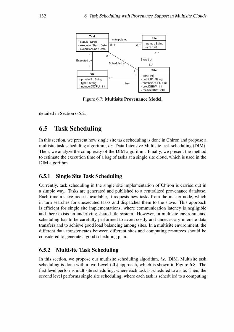
132 6. Task Scheduling with Provenance Support in Multisite Clouds
Figure 6.7: Multisite Provenance Model.
detailed in Section 6.5.2.
6.5 Task SchedulingIn this section, we present how single site task scheduling is done in Chiron and propose amultisite task scheduling algorithm, i.e. Data-Intensive Multisite task scheduling (DIM).Then, we analyze the complexity of the DIM algorithm. Finally, we present the methodto estimate the execution time of a bag of tasks at a single site cloud, which is used in theDIM algorithm.
6.5.1 Single Site Task SchedulingCurrently, task scheduling in the single site implementation of Chiron is carried out ina simple way. Tasks are generated and published to a centralized provenance database.Each time a slave node is available, it requests new tasks from the master node, whichin turn searches for unexecuted tasks and dispatches them to the slave. This approachis efficient for single site implementations, where communication latency is negligibleand there exists an underlying shared file system. However, in multisite environments,scheduling has to be carefully performed to avoid costly and unnecessary intersite datatransfers and to achieve good load balancing among sites. In a multisite environment, thedifferent data transfer rates between different sites and computing resources should beconsidered to generate a good scheduling plan.
6.5.2 Multisite Task SchedulingIn this section, we propose our mutlisite scheduling algorithm, i.e. DIM. Multisite taskscheduling is done with a two Level (2L) approach, which is shown in Figure 6.8. Thefirst level performs multisite scheduling, where each task is scheduled to a site. Then, thesecond level performs single site scheduling, where each task is scheduled to a computing
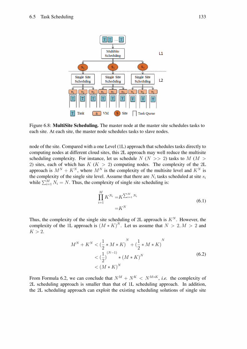
6.5 Task Scheduling 133
Figure 6.8: MultiSite Scheduling. The master node at the master site schedules tasks toeach site. At each site, the master node schedules tasks to slave nodes.
node of the site. Compared with a one Level (1L) approach that schedules tasks directly tocomputing nodes at different cloud sites, this 2L approach may well reduce the multisitescheduling complexity. For instance, let us schedule N (N >> 2) tasks to M (M >2) sites, each of which has K (K > 2) computing nodes. The complexity of the 2Lapproach is MN + KN , where MN is the complexity of the multisite level and KN isthe complexity of the single site level. Assume that there are Ni tasks scheduled at site siwhile
∑Mi=1 Ni = N . Thus, the complexity of single site scheduling is:
M∏i=1
KNi =K∑M
i=1 Ni
=KN
(6.1)
Thus, the complexity of the single site scheduling of 2L approach is KN . However, thecomplexity of the 1L approach is (M ∗K)N . Let us assume that N > 2,M > 2 andK > 2.
MN +KN < (12 ∗M ∗K)
N
+ (12 ∗M ∗K)
N
< (12)
(N−1)∗ (M ∗K)N
< (M ∗K)N
(6.2)
From Formula 6.2, we can conclude that NM + NK < NM∗K , i.e. the complexity of2L scheduling approach is smaller than that of 1L scheduling approach. In addition,the 2L scheduling approach can exploit the existing scheduling solutions of single site
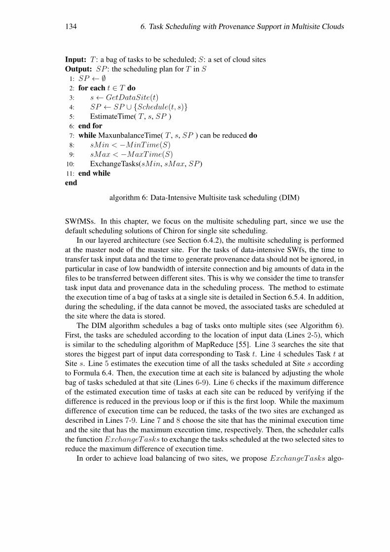
134 6. Task Scheduling with Provenance Support in Multisite Clouds
Input: T : a bag of tasks to be scheduled; S: a set of cloud sitesOutput: SP : the scheduling plan for T in S
1: SP ← ∅2: for each t ∈ T do3: s← GetDataSite(t)4: SP ← SP ∪ {Schedule(t, s)}5: EstimateTime( T , s, SP )6: end for7: while MaxunbalanceTime( T , s, SP ) can be reduced do8: sMin < −MinTime(S)9: sMax < −MaxTime(S)
10: ExchangeTasks(sMin, sMax, SP )11: end whileend
algorithm 6: Data-Intensive Multisite task scheduling (DIM)
SWfMSs. In this chapter, we focus on the multisite scheduling part, since we use thedefault scheduling solutions of Chiron for single site scheduling.
In our layered architecture (see Section 6.4.2), the multisite scheduling is performedat the master node of the master site. For the tasks of data-intensive SWfs, the time totransfer task input data and the time to generate provenance data should not be ignored, inparticular in case of low bandwidth of intersite connection and big amounts of data in thefiles to be transferred between different sites. This is why we consider the time to transfertask input data and provenance data in the scheduling process. The method to estimatethe execution time of a bag of tasks at a single site is detailed in Section 6.5.4. In addition,during the scheduling, if the data cannot be moved, the associated tasks are scheduled atthe site where the data is stored.
The DIM algorithm schedules a bag of tasks onto multiple sites (see Algorithm 6).First, the tasks are scheduled according to the location of input data (Lines 2-5), whichis similar to the scheduling algorithm of MapReduce [55]. Line 3 searches the site thatstores the biggest part of input data corresponding to Task t. Line 4 schedules Task t atSite s. Line 5 estimates the execution time of all the tasks scheduled at Site s accordingto Formula 6.4. Then, the execution time at each site is balanced by adjusting the wholebag of tasks scheduled at that site (Lines 6-9). Line 6 checks if the maximum differenceof the estimated execution time of tasks at each site can be reduced by verifying if thedifference is reduced in the previous loop or if this is the first loop. While the maximumdifference of execution time can be reduced, the tasks of the two sites are exchanged asdescribed in Lines 7-9. Line 7 and 8 choose the site that has the minimal execution timeand the site that has the maximum execution time, respectively. Then, the scheduler callsthe function ExchangeTasks to exchange the tasks scheduled at the two selected sites toreduce the maximum difference of execution time.
In order to achieve load balancing of two sites, we propose ExchangeTasks algo-
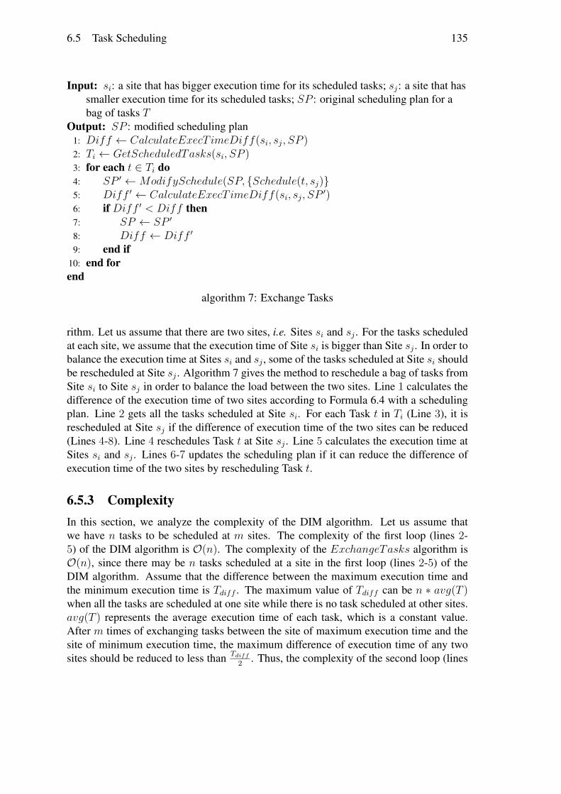
6.5 Task Scheduling 135
Input: si: a site that has bigger execution time for its scheduled tasks; sj: a site that hassmaller execution time for its scheduled tasks; SP : original scheduling plan for abag of tasks T
Output: SP : modified scheduling plan1: Diff ← CalculateExecT imeDiff(si, sj, SP )2: Ti ← GetScheduledTasks(si, SP )3: for each t ∈ Ti do4: SP ′ ←ModifySchedule(SP, {Schedule(t, sj)}5: Diff ′ ← CalculateExecT imeDiff(si, sj, SP ′)6: if Diff ′ < Diff then7: SP ← SP ′
8: Diff ← Diff ′
9: end if10: end forend
algorithm 7: Exchange Tasks
rithm. Let us assume that there are two sites, i.e. Sites si and sj . For the tasks scheduledat each site, we assume that the execution time of Site si is bigger than Site sj . In order tobalance the execution time at Sites si and sj , some of the tasks scheduled at Site si shouldbe rescheduled at Site sj . Algorithm 7 gives the method to reschedule a bag of tasks fromSite si to Site sj in order to balance the load between the two sites. Line 1 calculates thedifference of the execution time of two sites according to Formula 6.4 with a schedulingplan. Line 2 gets all the tasks scheduled at Site si. For each Task t in Ti (Line 3), it isrescheduled at Site sj if the difference of execution time of the two sites can be reduced(Lines 4-8). Line 4 reschedules Task t at Site sj . Line 5 calculates the execution time atSites si and sj . Lines 6-7 updates the scheduling plan if it can reduce the difference ofexecution time of the two sites by rescheduling Task t.
6.5.3 ComplexityIn this section, we analyze the complexity of the DIM algorithm. Let us assume thatwe have n tasks to be scheduled at m sites. The complexity of the first loop (lines 2-5) of the DIM algorithm is O(n). The complexity of the ExchangeTasks algorithm isO(n), since there may be n tasks scheduled at a site in the first loop (lines 2-5) of theDIM algorithm. Assume that the difference between the maximum execution time andthe minimum execution time is Tdiff . The maximum value of Tdiff can be n ∗ avg(T )when all the tasks are scheduled at one site while there is no task scheduled at other sites.avg(T ) represents the average execution time of each task, which is a constant value.After m times of exchanging tasks between the site of maximum execution time and thesite of minimum execution time, the maximum difference of execution time of any twosites should be reduced to less than Tdiff
2 . Thus, the complexity of the second loop (lines

136 6. Task Scheduling with Provenance Support in Multisite Clouds
6-9) of the DIM algorithm is O(m · n · log n). Therefore, the complexity of the DIMalgorithm is O(m · n · log n). It is only a little bit higher than that of OLB and MCT,which is O(m · n), but yields high reduction in SWf execution (see Section 6.6.3).
6.5.4 Execution Time EstimationWe now give the method to estimate the execution time of a bag of tasks at a single site,which is used in both the DIM algorithm and the MCT algorithm. Formula 6.3 gives theestimation of execution time without considering the time to generate provenance data,which is used in the MCT algorithm.
TotalT ime(T, s) =ExecT ime(T, s)+ InputTransT ime(T, s)
(6.3)
T represents the bag of tasks scheduled at site s. ExecT ime is the time to execute the bagof tasks T at site s, i.e. the time to run the corresponding programs. InputTransT imeis the time to transfer the input data of the tasks from other sites to site s. In the DIMalgorithm, we use Formula 6.4 to estimate the execution time with the consideration ofthe time to generate provenance data.
TotalT ime(T, s) =ExecT ime(T, s)+ InputTransT ime(T, s)+ ProvTransT ime(T, s)
(6.4)
ProvTransT ime is the time to generate provenance data in the provenance database.We assume that the workload of each task of the same activity is similar. The average
workload (in GFLOP) of the tasks of each activity and the computing capacity of eachVM at Site s is known to the system. The computing capacity (in GFLOPS) indicatesthe workload that can be realized per second. Then, the time to execute the tasks canbe estimated by dividing the total workload by the total computing capacity of Site s, asshown in Formula 6.5.
ExecT ime(T, s) = |T | ∗ AvgWorkload(T )∑VMi∈sComputingCapacity(VMi)
(6.5)
|T | represents the number of tasks in Bag T . AvgWorkload is the average workload ofthe bag of tasks.
The time to transfer input data can be estimated as the sum of the time to transfer theinput data from other sites to Site s as shown in Formula 6.6.
InTransT ime(T, s) =∑ti∈T
∑si∈S
InDataSize(ti, si)DataRate(si, s)
(6.6)
InDataSize(ti, si) represents the size of input data of Task ti, which is stored at Site si.

6.6 Experimental Evaluation 137
Figure 6.9: Buzz Workflow.
The size can be measured at runtime. DataRate(si, s) represents the data transfer rate,which can be configured by users. S represents the set of sites.
Finally, the time to generate provenance data is estimated by Formula 6.7.
ProvTransT ime(T, s) =|T | ∗ TransctionT imes(T )∗ AvgTransactionT ime(s)
(6.7)
|T | represents the number of tasks in Bag T . We can estimate AvgTransactionT imeby counting the time to perform a data exchange to update the provenance data of a taskin the provenance database from Site s. TransctionT imes(T ) represents the number ofdata exchanges to perform for generating the provenance data of each task in Bag T . Itcan be configured according to the features of the SWfMS.
6.6 Experimental EvaluationIn this section, we present an experimental evaluation of our DIM scheduling algorithmusing Microsoft Azure multisite cloud [5]. First, we present two real-life SWfs, i.e. Buzzand Montage, as use cases. Then, we explain the techniques for the implementation ofintersite communication of multisite Chiron in Azure. Afterwards, we show the exper-imental results of executing the two SWfs in Azure with different multisite schedulingalgorithms.
6.6.1 SWf Use CasesIn this section, we present two SWfs, i.e. Buzz and Montage, to evaluate our proposedalgorithms. The two SWfs have different structures, which can show that our proposedalgorithm is suitable for different SWfs.
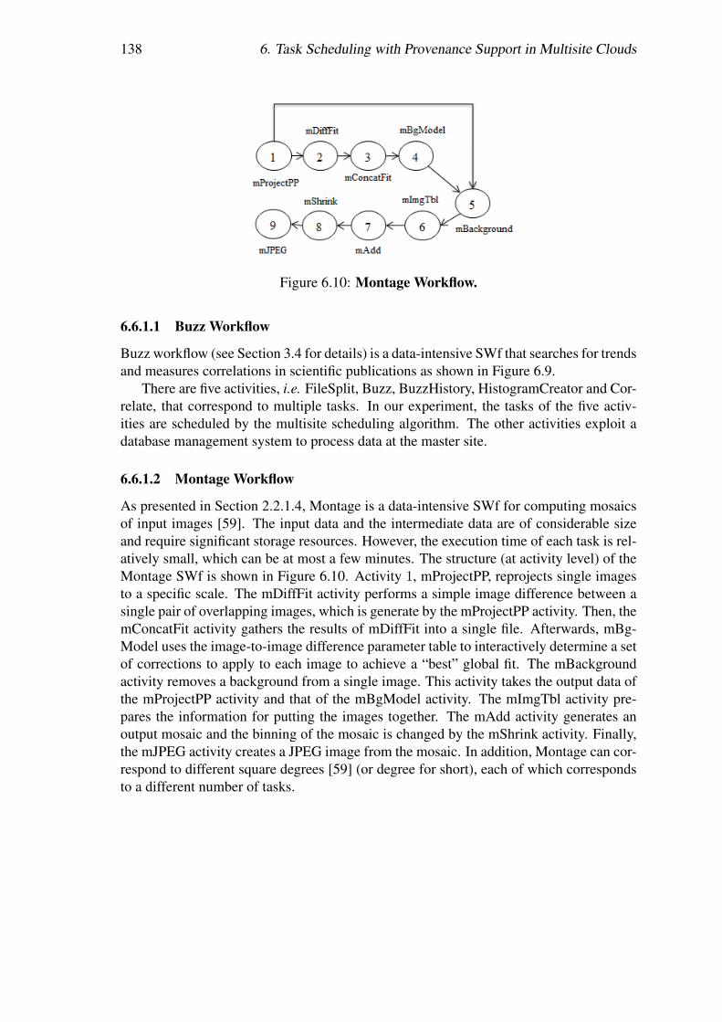
138 6. Task Scheduling with Provenance Support in Multisite Clouds
Figure 6.10: Montage Workflow.
6.6.1.1 Buzz Workflow
Buzz workflow (see Section 3.4 for details) is a data-intensive SWf that searches for trendsand measures correlations in scientific publications as shown in Figure 6.9.
There are five activities, i.e. FileSplit, Buzz, BuzzHistory, HistogramCreator and Cor-relate, that correspond to multiple tasks. In our experiment, the tasks of the five activ-ities are scheduled by the multisite scheduling algorithm. The other activities exploit adatabase management system to process data at the master site.
6.6.1.2 Montage Workflow
As presented in Section 2.2.1.4, Montage is a data-intensive SWf for computing mosaicsof input images [59]. The input data and the intermediate data are of considerable sizeand require significant storage resources. However, the execution time of each task is rel-atively small, which can be at most a few minutes. The structure (at activity level) of theMontage SWf is shown in Figure 6.10. Activity 1, mProjectPP, reprojects single imagesto a specific scale. The mDiffFit activity performs a simple image difference between asingle pair of overlapping images, which is generate by the mProjectPP activity. Then, themConcatFit activity gathers the results of mDiffFit into a single file. Afterwards, mBg-Model uses the image-to-image difference parameter table to interactively determine a setof corrections to apply to each image to achieve a “best” global fit. The mBackgroundactivity removes a background from a single image. This activity takes the output data ofthe mProjectPP activity and that of the mBgModel activity. The mImgTbl activity pre-pares the information for putting the images together. The mAdd activity generates anoutput mosaic and the binning of the mosaic is changed by the mShrink activity. Finally,the mJPEG activity creates a JPEG image from the mosaic. In addition, Montage can cor-respond to different square degrees [59] (or degree for short), each of which correspondsto a different number of tasks.

6.6 Experimental Evaluation 139
0
20
40
60
80
DIM MCT OLB0
5
10
15
Exec
utio
n tim
e (m
inut
e)
Tran
sfer
red
data
size
(MB)
Execution TimeData-transfer Size
Figure 6.11: Buzz SWf Execution time. The amount of data is 60MB.
6.6.2 Intersite CommunicationIn this section, we present the detailed techniques for the multisite file transfer moduleand multisite message communication module. We choose Azure Service Bus [2] torealize the functionality of message communication module. Azure Service Bus is ageneric, cloud-based messaging system for the communication among different devices.The communication can be based on the HTTP protocol, which does not need to maintainconnection information (HTTP is stateless). Although this may bring more overhead foreach message, the amount of control messages is low and this cost is negligible. The filetransfer module is realized by Java TCP connections between two master nodes of twodifferent sites. Since the idle intersite TCP connections may be cut down by the cloudoperator, e.g. every 5 − 10 minutes in Azure, the connections are maintained by sendingkeepalive messages. For instance, two messages per time period. Before execution,a task is scheduled at a site by the multisite task scheduler. If they are not stored atthe scheduled site, the input files of the task are transferred to the scheduled site by themultisite file transfer module.
6.6.3 ExperimentsThis section gives our experimental evaluation of the DIM algorithm, within MicrosoftAzure. Azure [5] has multiple cloud sites, e.g. Central US (CUS), West Europe (WEU)and North Europe (NEU). We instantiated three A4 (the type of VMs in Azure [8]) VMsat each of the three site, i.e. CUS, WEU and NEU. We take WEU as a master site.We deploy an A2 VM at WEU and install PostgreSQL database to manage provenancedata. We assume that the input data of the SWfs are distributed at the three sites. Wecompare our proposed algorithm with two representative baseline scheduling algorithms,i.e. Opportunistic Load Balancing (OLB) and Minimum Completion Time (MCT). In themultisite environment, OLB randomly selects a site for a task while MCT schedules atask to the site that can finish the execution first.
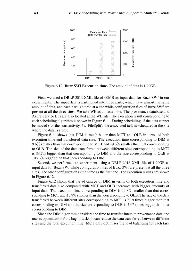
140 6. Task Scheduling with Provenance Support in Multisite Clouds
0
200
400
600
800
1000
DIM MCT OLB0
500
1000
1500
2000
Exec
utio
n tim
e (m
inut
e)
Tran
sfer
red
data
size
(MB)
Execution TimeData-transfer Size
Figure 6.12: Buzz SWf Execution time. The amount of data is 1.29GB.
First, we used a DBLP 2013 XML file of 60MB as input data for Buzz SWf in ourexperiments. The input data is partitioned into three parts, which have almost the sameamount of data, and each part is stored at a site while configuration files of Buzz SWf arepresent at all the three sites. We take WE as a master site. The provenance database andAzure Service Bus are also located at the WE site. The execution result corresponding toeach scheduling algorithm is shown in Figure 6.11. During scheduling, if the data cannotbe moved (for the start activity, i.e. FileSplit), the associated task is scheduled at the sitewhere the data is stored.
Figure 6.11 shows that DIM is much better than MCT and OLB in terms of bothexecution time and transferred data size. The execution time corresponding to DIM is9.6% smaller than that corresponding to MCT and 49.6% smaller than that correspondingto OLB. The size of the data transferred between different sites corresponding to MCTis 38.7% bigger than that corresponding to DIM and the size corresponding to OLB is108.6% bigger than that corresponding to DIM.
Second, we performed an experiment using a DBLP 2013 XML file of 1.29GB asinput data for Buzz SWf while configuration files of Buzz SWf are present at all the threesites. The other configuration is the same as the first one. The execution results are shownin Figure 6.12.
Figure 6.12 shows that the advantage of DIM in terms of both execution time andtransferred data size compared with MCT and OLB increases with bigger amounts ofinput data. The execution time corresponding to DIM is 24.3% smaller than that corre-sponding to MCT and 45.9% smaller than that corresponding to OLB. The size of the datatransferred between different sites corresponding to MCT is 7.19 times bigger than thatcorresponding to DIM and the size corresponding to OLB is 7.67 times bigger than thatcorresponding to DIM.
Since the DIM algorithm considers the time to transfer intersite provenance data andmakes optimization for a bag of tasks, it can reduce the data transferred between differentsites and the total execution time. MCT only optimizes the load balancing for each task

6.6 Experimental Evaluation 141
0
200
400
600
800
DIM MCT OLB0
200
400
600
Exec
utio
n tim
e (s
econ
d)
Tran
sfer
red
data
size
(MB)
Execution TimeData-transfer Size
Figure 6.13: Montage SWf Execution time. 0.5 degree.
among different sites without consideration of the time to transfer intersite provenancedata. It is a greedy algorithm that can reduce the execution time by balancing the ex-ecution time of each site while scheduling each task. However, it cannot optimize thescheduling for the whole execution of all the tasks of an activity. In addition, comparedwith OLB, MCT cannot reduce much the transferred data among different sites. SinceOLB simply tries to keep all the sites working on arbitrary tasks, it has the worst perfor-mance.
Furthermore, we executed the Montage SWf with 0.5 degree with three sites, i.e. CUS,WEU and NEU. The size of input data is 5.5GB. The input data is evenly partitioned tothree parts stored at the corresponding sites with configuration files stored at all the threesites. The execution time and amount of intersite transferred data corresponding to eachscheduling algorithm are shown in Figure 6.13.
The execution results of Montage with 0.5 degree reveals that the execution time ofDIM is 21.7% smaller than that of MCT and 37.1% smaller than that of OLB. This isexpected since DIM makes optimization for a bag of tasks in order to reduce intersitetransferred data with consideration of the time to transfer intersite intermediate data andprovenance data. MCT is optimized for load balancing only with consideration of in-termediate data. OLB has no optimization for load balancing. In addition, the intersitetransferred data of DIM is 42.3% bigger than that of MCT. Since DIM is designed toachieve load balancing of each site to reduce execution time, it may yield more intersitetransferred data in order to achieve load balance. However, the amount of intersite trans-ferred data of DIM is 28.6% smaller than that of OLB. This shows the efficiency of theoptimization for the data transfer of DIM. Moreover, when the degree (0.5) is low, there isless data to be processed by Montage, and the number of tasks to schedule is small. SinceDIM is designed for high numbers of tasks, the amounts of intersite transferred data arenot reduced very much in this situation.
Finally, we executed Montage SWf of 1 degree in the multisite cloud. We used thesame input data as in the previous experiment, i.e. 5.5GB input data evenly distributed at

142 6. Task Scheduling with Provenance Support in Multisite Clouds
0
300
600
900
1200
1500
DIM MCT OLB0
400
800
1200
1600
2000
2400
Exec
utio
n tim
e (s
econ
d)
Tran
sfer
red
data
size
(MB)
Execution TimeData-transfer Size
Figure 6.14: Montage SWf Execution time. 1 degree.
three sites. The execution time and the amount of intersite transferred data correspondingto each scheduling algorithm are shown in Figure 6.14.
The execution results of Montage with 1 degree reveals that the execution time of DIMis 16.4% smaller than that of MCT and 17.8% smaller than that of OLB. As explainedbefore, this is expected since DIM can reduce the execution time by balancing the loadamong different sites compared with MCT and OLB. In addition, the intersite transferreddata of DIM is 10.7% bigger than that of MCT. This is much smaller than the valuefor 0.5 degree (42.3%), since there are more tasks to schedule when the degree is 1 andDIM reduces intersite transferred data for a big amount of tasks. However, the amountof intersite transferred data is bigger than that of MCT. This happens since the mainobjective of DIM is to reduce execution time instead of reducing intersite transferreddata. In addition, the amount of intersite transferred data of DIM is 33.4% smaller thanthat of OLB, which shows the efficiency of the optimization for the data transfer of DIM.
Table 6.1: Scheduling Time. The unit of time is second. The size of the input data ofBuzz SWf is 1.2GB and the degree of Montage is 13.
Algorithm DIM MCT OLBBuzz 633 109 17
Montage 29.2 28.8 1.5
In addition, we measured the time to execute the scheduling algorithms to generatescheduling plans while executing Buzz and Montage. The scheduling time is shown inTable 6.1. The complexity of MCT is the same as that of OLB, which is O(m · n).However, the scheduling time of MCT is much bigger than OLB. The reason is that MCTneeds to interact with the provenance database to get the information of the files in orderto estimate the time to transfer the files among different sites. The table shows that thetime to execute DIM is much higher than OLB for both Buzz and Montage since thecomplexity of DIM is higher than that of OLB and that DIM has more interactions with
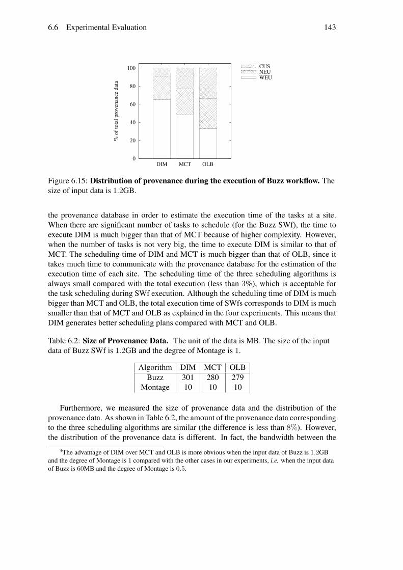
6.6 Experimental Evaluation 143
0
20
40
60
80
100
DIM MCT OLB
% o
f tot
al p
rove
nanc
e da
ta
WEUNEUCUS
Figure 6.15: Distribution of provenance during the execution of Buzz workflow. Thesize of input data is 1.2GB.
the provenance database in order to estimate the execution time of the tasks at a site.When there are significant number of tasks to schedule (for the Buzz SWf), the time toexecute DIM is much bigger than that of MCT because of higher complexity. However,when the number of tasks is not very big, the time to execute DIM is similar to that ofMCT. The scheduling time of DIM and MCT is much bigger than that of OLB, since ittakes much time to communicate with the provenance database for the estimation of theexecution time of each site. The scheduling time of the three scheduling algorithms isalways small compared with the total execution (less than 3%), which is acceptable forthe task scheduling during SWf execution. Although the scheduling time of DIM is muchbigger than MCT and OLB, the total execution time of SWfs corresponds to DIM is muchsmaller than that of MCT and OLB as explained in the four experiments. This means thatDIM generates better scheduling plans compared with MCT and OLB.
Table 6.2: Size of Provenance Data. The unit of the data is MB. The size of the inputdata of Buzz SWf is 1.2GB and the degree of Montage is 1.
Algorithm DIM MCT OLBBuzz 301 280 279
Montage 10 10 10
Furthermore, we measured the size of provenance data and the distribution of theprovenance data. As shown in Table 6.2, the amount of the provenance data correspondingto the three scheduling algorithms are similar (the difference is less than 8%). However,the distribution of the provenance data is different. In fact, the bandwidth between the
3The advantage of DIM over MCT and OLB is more obvious when the input data of Buzz is 1.2GBand the degree of Montage is 1 compared with the other cases in our experiments, i.e. when the input dataof Buzz is 60MB and the degree of Montage is 0.5.
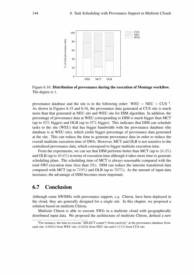
144 6. Task Scheduling with Provenance Support in Multisite Clouds
0
20
40
60
80
100
DIM MCT OLB
% o
f tot
al p
rove
nanc
e da
ta
WEUNEUCUS
Figure 6.16: Distribution of provenance during the execution of Montage workflow.The degree is 1.
provenance database and the site is in the following order: WEU > NEU > CUS 4.As shown in Figures 6.15 and 6.16, the provenance data generated at CUS site is muchmore than that generated at NEU site and WEU site for DIM algorithm. In addition, thepercentage of provenance data at WEU corresponding to DIM is much bigger than MCT(up to 95% bigger) and OLB (up to 97% bigger). This indicates that DIM can scheduletasks to the site (WEU) that has bigger bandwidth with the provenance database (thedatabase is at WEU site), which yields bigger percentage of provenance data generatedat the site. This can reduce the time to generate provenance data in order to reduce theoverall multisite execution time of SWfs. However, MCT and OLB is not sensitive to thecentralized provenance data, which correspond to bigger multisite execution time.
From the experiments, we can see that DIM performs better than MCT (up to 24.3%)and OLB (up to 49.6%) in terms of execution time although it takes more time to generatescheduling plans. The scheduling time of MCT is always reasonable compared with thetotal SWf execution time (less than 3%). DIM can reduce the intersite transferred datacompared with MCT (up to 719%) and OLB (up to 767%). As the amount of input dataincreases, the advantage of DIM becomes more important.
6.7 ConclusionAlthough some SWfMSs with provenance support, e.g. Chiron, have been deployed inthe cloud, they are generally designed for a single site. In this chapter, we proposed asolution based on multisite Chiron.
Multisite Chiron is able to execute SWfs in a multisite cloud with geographicallydistributed input data. We proposed the architecture of multisite Chiron, defined a new
4For instance, the time to execute "SELECT count(*) from eactivity" at the provenance database fromeach site: 0.0027s from WEU site, 0.0253s from NEU site and 0.1117s from CUS site.

6.7 Conclusion 145
provenance model for multisite SWf execution and a global method to gather the dis-tributed provenance data in a centralized database. Based on this architecture, we pro-posed a new scheduling algorithm, i.e. DIM, which considers the latency to transfer dataand to generate provenance data in multisite cloud. We analyzed the complexity of DIM(O(m · n · log n)), which is quite acceptable for scheduling bags of tasks. We used tworeal-life SWfs, i.e. Buzz and Montage to evaluate the DIM algorithm in Microsoft Azurewith three sites. The experiments show that although its complexity is higher than thatof OLB and MCT, DIM is much better than two representative baseline algorithms, i.e.MCT (up to 24.3%) and OLB (up to 49.6%), in terms of execution time. In addition,DIM can also reduce significantly data transfer between sites, compared with MCT (up to719%) and OLB (up to 767%). Moreover, the scheduling time of MCT is always reason-able compared with the total SWf execution time (less than 3%). The advantage of DIMbecomes important with high numbers of tasks.


Chapter 7
Conclusions
In this thesis, we addressed the problem of executing data-intensive SWfs in a multisitecloud, where the data and computing resources may be distributed in different cloud sites.To this end, we proposed a distributed and parallel approach that leverages the resourcesavailable at different cloud sites, based on a survey of existing techniques. In the sur-vey, we proposed a functional SWfMS architecture by analyzing and categorizing theexisting techniques. To exploit parallelism, we used an algebraic approach, which al-lows expressing SWf activities using operators and automatically transforming them intomultiple tasks. We proposed SWf partitioning algorithms, a dynamic VM provisioningalgorithm, an activity scheduling algorithm and a task scheduling algorithm. DifferentSWf partitioning algorithms partition a SWf to several fragments. The VM provisioningalgorithm is used to dynamically create an optimal combination of VMs for executingSWf fragments at each cloud site. The activity scheduling algorithm distributes the SWffragments to the cloud sites with the minimum cost based on a multi-objective cost model.The task scheduling algorithm directly distributes tasks among different cloud sites whileachieving load balancing at each site based on a multisite SWfMS. We evaluated our pro-posed solutions by executing real-life SWfs in the Microsoft Azure cloud, the results ofwhich shown the advantages of our solutions over the existing techniques. In this chap-ter, we summarize and discuss the contributions made in this thesis. Then, we give someresearch directions for future work.
7.1 ContributionsA survey of existing techniques for SWfs execution.
We discussed the existing techniques for parallel execution of data-intensive SWfs indifferent infrastructures, especially in the cloud. First, we introduced the definitions inSWf management, including SWfs and SWfMSs. Then, we presented in more detailsa five-layer functional architecture of SWfMSs and the corresponding functions. Specialattention has been paid to data-intensive SWfs by identifying their features and presentingthe corresponding techniques. Second, we presented the basic techniques for the parallel
147

148 7. Conclusions
execution of SWfs in SWfMSs: parallelization and scheduling. We showed how differ-ent kinds of parallelism (coarse-grained parallelism, data parallelism, independent paral-lelism and pipeline parallelism) can be exploited for parallelizing SWfs. The schedulingmethods to allocate tasks to computing resources can be static or dynamic, with differenttrade-offs, or hybrid to combine the advantages of static and dynamic scheduling meth-ods. SWf scheduling may include an optimization phase to minimize a multi-objectivefunction, in a given context (cluster, grid, cloud). Third, we discussed cloud computingand the basic techniques for parallel execution of SWfs in the cloud, including singlesite cloud and multisite cloud. We discussed three categories of cloud computing, multi-site management in the cloud and data storage in the cloud. The data storage techniquesinclude shared-disk file systems and distributed file systems. Then, we analyzed the par-allelization techniques of SWfs in both single site cloud and multisite cloud. Fourth, toillustrate the use of the techniques, we introduced the recent parallelization frameworkssuch as MapReduce and gave a comparative analysis of eight popular SWfMSs (Pega-sus, Swift, Kepler, Taverna, Chiron, Galaxy, Triana and Askalon) and a science gatewayframework (WS-PGRADE/gUSE). Finally, we identified the limitations of existing tech-niques and proposed some research issues.
SWf Partitioning for the Execution in a Multisite Cloud.
We tackled the problem of SWf partitioning problem in order to execute SWfs in a mul-tisite cloud. Our main objective was to enable SWf execution in a multisite cloud by par-titioning SWfs into fragments while ensuring some activities executed at specific cloudsites. First, we presented the general SWf partitioning techniques, i.e. data partitioningand DAG partitioning. Then, we focused on DAG partitioning and mentioned activity en-capsulation technique. Afterward, we proposed our SWf partitioning methods, namelyScientist Privacy (SPr), Data Transfer Minimization (DTM) and Computing CapacityAdaptation (CCA). SPr partitions SWfs by putting locking activities and its availablefollowing activities to a fragment, in order to better support execution monitoring undersecurity restriction. DTM partitions SWfs with the consideration of locking activitieswhile minimizing the volume of data to be transferred among different SWf fragments.CCA partitions SWfs according to the computing capacity of different cloud sites. Thistechnique tries to put more activities to the fragment to be executed within a cloud sitewith bigger computing capacity. Our proposed partitioning techniques are suitable fordifferent configurations of clouds in order to reduce SWf execution time. In addition, wealso proposed to use data refining techniques, namely, file combining and data compres-sion, to reduce the time to transfer data among different sites.
We evaluated extensively our proposed partitioning techniques by executing the BuzzSWf at two sites, i.e. Western Europe and Eastern US, of the Azure cloud with differ-ent configurations. All the sites have the same amounts and types of VMs correspond tothe homogeneous configuration while the sites have different amounts or types of VMscorrespond to the heterogeneous configuration. The experimental results show that DTMwith data refining techniques is suitable (24.1% of time saved compared to CCA withoutdata refining) for executing SWfs in a multisite cloud with a homogeneous configuration,

7.1 Contributions 149
and that CCA performs better (28.4% of time saved compared to SPr technique withoutdata refining) with a heterogeneous configuration. In addition, the results also reveal thatdata refining techniques can significantly reduce the time to transfer data between twodifferent sites.
VM Provisioning in a Single Site Cloud.
We handled the problem of generating VM provisioning plans for SWf execution withina single cloud site for multiple objectives. Our main contribution was to propose a costmodel and an algorithm in order to generate VM provisioning plans to reduce both exe-cution time and monetary cost for SWf execution in a single site cloud. To address theproblem, we designed a multi-objective cost model for the execution of SWfs within asingle cloud site. The cost model is a weighted function with the objectives of reducingexecution time and monetary cost. Our cost model takes the sequential workload andthe cost to start VMs into consideration, which is more precise compared with existingcost models. Then, based on the cost model, we proposed Single Site VM Provisioning(SSVP) algorithm to generate provisioning plans for SWf execution within a single cloudsite. The SSVP first calculates an optimal number of CPU cores for SWf execution. Then,it generates a provisioning plan and iteratively improves the provisioning plan in order toreduce the cost based on the cost model and the optimal number of CPU cores.
We made extensive evaluations to compare our cost model and algorithm with anexisting approach, i.e. GraspCC. We executed SciEvol with different amounts of inputdata and different weights of execution time at the Japan East site of Azure cloud. Theexperimental results show that our algorithm can adapt VM provisioning plans to differentconfigurations, i.e. different weights of execution time and generate better (53.6%) VMprovisioning plans compared with GraspCC. The results also reveal that our cost modelis more (76.7%) precise to estimate the execution time and the monetary cost comparedwith the existing approach.
Multi-Objective SWf Fragment Scheduling in a Multisite cloud.
We addressed the problem of SWf fragment scheduling for multiple objectives in orderto enable SWf execution in a multisite cloud with a stored data constraint. In this work,we took into consideration of different prices to use VMs and stored data at differentsites. We formally defined the scheduling problem of executing SWfs in a multisite cloudfor multiple objectives with the stored data constraint. Then, we presented the systemmodel for multisite SWf execution. Afterward, we detailed our multi-objective cost modelcomposed of a weighted function with two objectives, i.e reducing execution time andmonetary cost. In addition, the cost model considers different costs of using VMs atdifferent cloud sites. Finally, we presented two adapted scheduling algorithms, i.e. datalocation based scheduling (LocBased) and site greedy scheduling (SGreedy), and ourproposed algorithm, namely activity greedy scheduling (ActGreedy). LocBased exploitsDTM to partition SWfs and schedules the fragments to the site where its input data isstored. This algorithm does not take the monetary cost into consideration and may incur a
150 7. Conclusions
big cost to execute SWfs. SGreedy takes advantage of the activity encapsulation techniqueto partition SWfs and schedules the best fragment for each site. SGreedy schedules theactivities of a pipeline of activities to different sites, which leads to bigger intersite datatransfer and execution time. ActGreedy partitions SWfs with the activity encapsulationtechnique and groups small fragments to bigger fragments to reduce data transfer amongdifferent sites and schedules each fragment to the best site. This algorithm can reduce theoverall execution time by comparing the cost to execute fragments at each site, which isgenerated based on the SSVP algorithm.
We evaluated our scheduling algorithm by executing SciEvol with different amountsof input data and different weights of objectives at three cloud sites of Azure. The threecloud sites are West Europe, Japan West, and Japan East and the costs of using VMs ateach site are different. We used SSVP to generate VM provisioning plans to execute SWffragments at each site. The experimental results shown that ActGreedy performs better interms of the weighted cost to execute SWfs in a multisite cloud compared with LocBased(up to 10.7%) and SGreedy (up to 17.2%). In addition, the results also reveal that thescheduling time of ActGreedy is reasonable compared with two general approaches.
Multisite Chiron and Multisite Task Scheduling with Provenance Support.
We dealt with task scheduling problem for multisite SWf execution with provenance sup-port. The main goal was to enable SWf execution with the distributed input data at differ-ent sites within the minimum time with provenance support while the bandwidths amongdifferent sites are different. In this work, we formally defined the task scheduling problemfor multisite SWf execution, including the support for provenance data, different band-widths among different sites and the distribution of input data. Then, we proposed multi-site Chiron, which enables scheduling and executing tasks of one activity at different siteswith a centralized provenance database. We also detailed the modifications made to adaptsingle site Chiron to multisite. Then, we proposed our two level scheduling and our inter-site task scheduling algorithm, i.e. Data-Intensive Multisite task scheduling (DIM). DIMconsiders the data locality and different bandwidths among different sites while transfer-ring intersite provenance data. DIM also achieves load balance among different sites forthe task execution based on an execution time estimation method.
We evaluated our algorithms and multisite Chiron by executing Buzz and Montage inthree Azure cloud sites, i.e. Central US, West Europe and North Europe. We executedBuzz with different amounts of input data and Montage with different degrees using themultisite Chiron. The experimental results show that DIM performs much better than twoexisting scheduling algorithms, i.e. MCT (up to 24.3%) and OLB (up to 49.6%), in termsof execution time. Moreover, DIM can also reduce significantly (up to more than 7 times)data transfer between sites, compared with MCT and OLB. In addition, the results alsoreveal that the scheduling time of DIM is reasonable compared with the overall executiontime of SWfs (less than 3%). In particular, the experiments show that the distribution oftasks is adapted according to different bandwidths among different sites for the generationof provenance data.
7.2 Directions for Future Work 151
7.2 Directions for Future WorkOur contributions can be used as a starting point for future research. With big data beingproduced and to be processed at different sites of the cloud, multisite management of SWfexecution in the cloud becomes more and more important. Based on this thesis’ results,we can propose some future research directions:
• Provenance distribution. The existing SWfMSs generally store the provenancedata in a centralized way and stores the data at a centralized site. This may incurnetwork congestion when large amounts of tasks are executed in parallel. Thus,we believe that distributed provenance data management can reduce the time togenerate or retrieve data at each site in order to reduce the overall SWf executiontime in a multisite cloud. In addition, with data replication approaches in the dis-tributed provenance data architecture, we believe that this approach can also helpfault-tolerance at the multisite level, i.e. the situation where a cloud site is down.
• Data transfer. The data transfer between two sites is generally achieved by havingtwo nodes, each at one of the two sites, communicating directly. This method isnot efficient in a multisite cloud. One possible solution is to select several nodes ateach site to send or receive data, by exploiting parallel data transfer and making thedata transfer more efficient. Then, the problem of matching the nodes at two cloudsites is critical for the multisite data transfer rate.
• Multisite Spark. Because of in-memory data processing, Spark has become a ma-jor framework for big data processing. Spark can be used as an engine to executeSWfs. However, Spark is designed for a single cluster environment, where thebandwidth among different computing nodes are high and similar. Thus, it is in-teresting to propose multisite scheduling algorithms and optimizations to use Sparkfor multisite SWf execution. In addition, the problem of VM provisioning for Sparkclusters in the cloud also remains critical to use Spark in a multisite cloud.
• Architecture. The structure of SWfMSs is generally centralized, with a masternode, which is a single point of failure and performance bottleneck, managing allthe optimization and scheduling processes. In addition, the system models (seeChapter 3, 5, 6) presented in this thesis are based on a master-worker model. Apeer-to-peer architecture can be used in order to achieve fault-tolerance during theexecution of SWfs both within a single site cloud or a multisite cloud. With apeer-to-peer architecture and data replication approaches, we believe the multisiteSWfMSs are robust enough to address the situation where one computing node isdown or even a cloud site is down.
• Dynamic Scheduling. The scheduling algorithms generally schedule activities ortasks according to predefined parameters with a static scheduling approach. How-ever, the workload or the features of VMs are dynamically varying at each site of thecloud. We believe that dynamic scheduling of activities or tasks can perform better

152 7. Conclusions
with the parameters measured during SWf execution in terms of execution time,monetary cost, energy consumption, and others for SWf execution in a multisitecloud.
Bibliography
[1] Alice Collaboration. http://aliceinfo.cern.ch/general/index.html.
[2] Azure service bus. http://azure.microsoft.com/en-us/services/service-bus/.
[3] Computing capacity for a CPU. http://en.community.dell.com/techcenter/high-performance-computing/w/wiki/2329.
[4] DBLP Computer Science Bibliography. http://dblp.uni-trier.de/.
[5] Microsoft Azure. http://azure.microsoft.com.
[6] Montage. http://montage.ipac.caltech.edu/docs/gridtools.html.
[7] Oma genome database. http://omabrowser.org/All/eukaryotes.cdna.fa.gz.
[8] Parameters of different types of vms in microsoft Azure. https://azure.microsoft.com/en-us/pricing/details/virtual-machines/.
[9] Sequence identifier. http://omabrowser.org/All/oma-groups.txt.gz.
[10] VM bandwidth in Azure. http://windowsazureguide.net/tag/auzre-virtual-machines-sizes-bandwidth/.
[11] VM parameters in Azure. http://msdn.microsoft.com/en-us/library/azure/dn197896.aspx.
[12] Amazon cloud. http://aws.amazon.com/, 2015.
[13] Grid’5000 project. https://www.grid5000.fr/mediawiki/index.php, 2015.
[14] Microsoft Azure cloud. http://azure.microsoft.com/, 2015.
153

154 7. Bibliography
[15] Pegasus 4.4.1 user guide. https://pegasus.isi.edu/wms/docs/latest/, 2015.
[16] ABOUELHODA, M., ISSA, S., AND GHANEM, M. Tavaxy: Integrating tavernaand galaxy workflows with cloud computing support. BMC Bioinformatics 13, 1(2012), 77.
[17] AFGAN, E., BAKER, D., CORAOR, N., CHAPMAN, B., NEKRUTENKO, A., AND
TAYLOR, J. Galaxy cloudman: delivering cloud compute clusters. BMC Bioinfor-matics 11, Suppl 12 (2010), S4.
[18] ALBRECHT, M., DONNELLY, P., BUI, P., AND THAIN, D. Makeflow: A portableabstraction for data intensive computing on clusters, clouds, and grids. In 1st ACMSIGMOD Workshop on Scalable Workflow Execution Engines and Technologies(2012), pp. 1:1–1:13.
[19] ALTINTAS, I., BARNEY, O., AND JAEGER-FRANK, E. Provenance collectionsupport in the kepler scientific workflow system. In Int. Conf. on Provenance andAnnotation of Data (2006), pp. 118–132.
[20] ALTINTAS, I., BERKLEY, C., JAEGER, E., JONES, M., LUDASCHER, B., AND
MOCK, S. Kepler: an extensible system for design and execution of scientificworkflows. In 16th Int. Conf. on Scientific and Statistical Database Management(SSDBM) (2004), pp. 423–424.
[21] ALTINTAS, I., BERKLEY, C., JAEGER, E., JONES, M., LUDÄSCHER, B., AND
MOCK, S. Kepler: Towards a Grid-Enabled system for scientific workflows.The Workflow in Grid Systems Workshop in GGF10-The 10th Global Grid Forum(2004).
[22] ANGLANO, C., AND CANONICO, M. Scheduling algorithms for multiple bag-of-task applications on desktop grids: A knowledge-free approach. In 22nd IEEE Int.Symposium on Parallel and Distributed Processing (IPDPS) (2008), pp. 1–8.
[23] ARKOUDAS, K., ZEE, K., KUNCAK, V., AND RINARD, M. Verifying a file sys-tem implementation. In 6th Int. Conf. on Formal Engineering Methods (ICFEM),vol. 3308. 2004, pp. 373–390.
[24] BALASKÓ, Á. Workflow concept of ws-pgrade/guse. In Science Gateways forDistributed Computing Infrastructures, P. Kacsuk, Ed. Springer International Pub-lishing, 2014, pp. 33–50.
[25] BARKER, A., AND HEMERT, J. V. Scientific workflow: A survey and research di-rections. In 7th Int. Conf. on Parallel Processing and Applied Mathematics (2008),pp. 746–753.

155
[26] BELHAJJAME, K., CRESSWELL, S., GIL, Y., GOLDEN, R., GROTH, P., KLYNE,G., MCCUSKER, J., MILES, S., MYERS, J., AND SAHOO, S. The provdata model and abstract syntax notation. http://www.w3.org/TR/2011/WD-prov-dm-20111215/, 2011.
[27] BERGMANN, R., AND GIL, Y. Retrieval of semantic workflows with knowledgeintensive similarity measures. In 19th Int. Conf. on Case-Based Reasoning Re-search and Development (2011), pp. 17–31.
[28] BHUVANESHWAR, K., SULAKHE, D., GAUBA, R., RODRIGUEZ, A., MADDURI,R., DAVE, U., LACINSKI, L., FOSTER, I., GUSEV, Y., AND MADHAVAN, S. Acase study for cloud based high throughput analysis of {NGS} data using the globusgenomics system. Computational and Structural Biotechnology Journal 13 (2015),64 – 74.
[29] BLAGODUROV, S., FEDOROVA, A., VINNIK, E., DWYER, T., AND HERMENIER,F. Multi-objective job placement in clusters. In Proceedings of the Int. Conf.for High Performance Computing, Networking, Storage and Analysis, SC (2015),pp. 66:1–66:12.
[30] BLYTHE, J., JAIN, S., DEELMAN, E., GIL, Y., VAHI, K., MANDAL, A., AND
KENNEDY, K. Task scheduling strategies for workflow-based applications in grids.In 5th IEEE Int. Symposium on Cluster Computing and the Grid (CCGrid) (2005),pp. 759–767.
[31] BOUGANIM, L., FABRET, F., MOHAN, C., AND VALDURIEZ, P. Dynamic queryscheduling in data integration systems. In International Conference on Data Engi-neering (ICDE) (2000), pp. 425–434.
[32] BRANDIC, I., AND DUSTDAR, S. Grid vs cloud - A technology comparison. it -Information Technology 53, 4 (2011), 173–179.
[33] BUX, M., AND LESER, U. Parallelization in scientific workflow managementsystems. The Computing Research Repository (CoRR) abs/1303.7195 (2013).
[34] CALA, J., XU, Y., WIJAYA, E., AND MISSIER, P. From scripted hpc-based NGSpipelines to workflows on the cloud. In 14th IEEE/ACM Int. Symposium on Cluster,Cloud and Grid Computing (CCGrid) (2014), pp. 694–700.
[35] CARPENTER, B., GETOV, V., JUDD, G., SKJELLUM, A., AND FOX, G. Mpj:Mpi-like message passing for java. Concurrency and Computation: Practice andExperience 12, 11 (2000), 1019–1038.
[36] CHANG, D., SON, J. H., AND KIM, M. Critical path identification in the contextof a workflow. Information & Software Technology 44, 7 (2002), 405–417.
156 7. Bibliography
[37] CHEN, W., AND DEELMAN, E. Integration of workflow partitioning and resourceprovisioning. In IEEE/ACM Int. Symposium on Cluster Computing and the Grid(CCGRID) (2012), pp. 764–768.
[38] CHEN, W., AND DEELMAN, E. Partitioning and scheduling workflows acrossmultiple sites with storage constraints. In 9th Int. Conf. on Parallel Processing andApplied Mathematics - Volume Part II (2012), vol. 7204, pp. 11–20.
[39] CHEN, W., SILVA, R. D., DEELMAN, E., AND SAKELLARIOU, R. Balancedtask clustering in scientific workflows. In IEEE 9th Int. Conf. on e-Science (2013),pp. 188–195.
[40] CHERVENAK, A. L., SMITH, D. E., CHEN, W., AND DEELMAN, E. Integrat-ing policy with scientific workflow management for data-intensive applications.In Supercomputing (SC) Companion: High Performance Computing, NetworkingStorage and Analysis (2012), pp. 140–149.
[41] CHIRIGATI, F., SILVA, V., OGASAWARA, E., DE OLIVEIRA, D., DIAS, J.,PORTO, F., VALDURIEZ, P., AND MATTOSO, M. Evaluating parameter sweepworkflows in high performance computing. In 1st ACM SIGMOD Workshop onScalable Workflow Execution Engines and Technologies (2012), pp. 2:1–2:10.
[42] CHOWDHURY, M., ZAHARIA, M., MA, J., JORDAN, M. I., AND STOICA, I.Managing data transfers in computer clusters with orchestra. ACM SIGCOMMConf. on Applications, Technologies, Architectures, and Protocols for ComputerCommunications 41, 4 (2011), 98–109.
[43] COALITION, W. M. Workflow management coalition terminology and glossary,1999.
[44] COHEN-BOULAKIA, S., CHEN, J., MISSIER, P., GOBLE, C. A., WILLIAMS,A. R., AND FROIDEVAUX, C. Distilling structure in taverna scientific workflows:a refactoring approach. BMC Bioinformatics 15, S-1 (2014), S12.
[45] COSTA, F., DE OLIVEIRA, D., OCALA, K., OGASAWARA, E., DIAS, J., AND
MATTOSO, M. Handling failures in parallel scientific workflows using clouds.In Supercomputing (SC) Companion: High Performance Computing, NetworkingStorage and Analysis (2012), pp. 129–139.
[46] COSTA, F., SILVA, V., DE OLIVEIRA, D., OCAÑA, K. A. C. S., OGASAWARA,E. S., DIAS, J., AND MATTOSO, M. Capturing and querying workflow runtimeprovenance with prov: a practical approach. In EDBT/ICDT Workshops (2013),pp. 282–289.

157
[47] COUTINHO, R., DRUMMOND, L., FROTA, Y., DE OLIVEIRA, D., AND OCANA,K. Evaluating grasp-based cloud dimensioning for comparative genomics: A prac-tical approach. In 2014 IEEE Int. Conf. on Cluster Computing (CLUSTER) (2014),pp. 371–379.
[48] CRAWL, D., WANG, J., AND ALTINTAS, I. Provenance for mapreduce-baseddata-intensive workflows. In 6th Workshop on Workflows in Support of Large-scaleScience (2011), pp. 21–30.
[49] CRITCHLOW, T., AND JR., G. C. Supercomputing and scientific workflows gapsand requirements. In World Congress on Services (2011), pp. 208–211.
[50] DE OLIVEIRA, D., OCAÑA, K. A. C. S., BAIÃO, F., AND MATTOSO, M. Aprovenance-based adaptive scheduling heuristic for parallel scientific workflows inclouds. Journal of Grid Computing 10, 3 (2012), 521–552.
[51] DE OLIVEIRA, D., OGASAWARA, E., BAIÃO, F., AND MATTOSO, M. Scicumu-lus: A lightweight cloud middleware to explore many task computing paradigmin scientific workflows. In 3rd Int. Conf. on Cloud Computing (CLOUD) (2010),pp. 378–385.
[52] DE OLIVEIRA, D., OGASAWARA, E., OCAÑA, K., BAIÃO, F., AND MATTOSO,M. An adaptive parallel execution strategy for cloud-based scientific workflows.Concurrency and Computation: Practice & Experience 24, 13 (2012), 1531–1550.
[53] DE OLIVEIRA, D., VIANA, V., OGASAWARA, E., OCANA, K., AND MATTOSO,M. Dimensioning the virtual cluster for parallel scientific workflows in clouds. In4th ACM Workshop on Scientific Cloud Computing (2013), pp. 5–12.
[54] DE OLIVEIRA, D., VIANA, V., OGASAWARA, E. S., OCAÑA, K. A. C. S., AND
MATTOSO, M. Dimensioning the virtual cluster for parallel scientific workflowsin clouds. In ScienceCloud’13, Proceedings of the 4th ACM HPDC Workshop onScientific Cloud Computing (2013), pp. 5–12.
[55] DEAN, J., AND GHEMAWAT, S. Mapreduce: Simplified data processing on largeclusters. In 6th Symposium on Operating System Design and Implementation(OSDI 2004) (2004), pp. 137–150.
[56] DEELMAN, E., CALLAGHAN, S., FIELD, E., FRANCOEUR, H., GRAVES, R.,GUPTA, N., GUPTA, V., JORDAN, T. H., KESSELMAN, C., MAECHLING, P.,MEHRINGER, J., MEHTA, G., OKAYA, D., VAHI, K., AND ZHAO, L. Managinglarge-scale workflow execution from resource provisioning to provenance tracking:The cybershake example. In Second Int. Conf. on e-Science and Grid Technologies(2006), p. 14.

158 7. Bibliography
[57] DEELMAN, E., GANNON, D., SHIELDS, M., AND TAYLOR, I. Workflows ande-science: An overview of workflow system features and capabilities. Future Gen-eration Computer Systems 25, 5 (2009), 528–540.
[58] DEELMAN, E., JUVE, G., AND BERRIMAN, G. B. Using clouds for science, isit just kicking the can down the road? In Cloud Computing and Services Sci-ence (CLOSER), 2nd Int. Conf. on Cloud Computing and Services Science (2012),pp. 127–134.
[59] DEELMAN, E., SINGH, G., LIVNY, M., BERRIMAN, B., AND GOOD, J. The costof doing science on the cloud: The montage example. In ACM/IEEE Conf. on HighPerformance Computing (2008), pp. 1–12.
[60] DEELMAN, E., SINGH, G., SU, M.-H., BLYTHE, J., GIL, Y., KESSELMAN,C., MEHTA, G., VAHI, K., BERRIMAN, G. B., GOOD, J., LAITY, A., JACOB,J. C., AND KATZ, D. S. Pegasus: A framework for mapping complex scientificworkflows onto distributed systems. Scientific Programming 13, 3 (2005), 219–237.
[61] DEELMAN, E., VAHI, K., JUVE, G., RYNGE, M., CALLAGHAN, S., MAECH-LING, P. J., MAYANI, R., CHEN, W., D. SILVA, R. F., LIVNY, M., AND
WENGER, K. Pegasus: a workflow management system for science automation.Future Generation Computer Systems (2014).
[62] DENG, K., KONG, L., SONG, J., REN, K., AND YUAN, D. A weighted k-meansclustering based co-scheduling strategy towards efficient execution of scientificworkflows in collaborative cloud environments. In IEEE 9th Int. Conf. on De-pendable, Autonomic and Secure Computing (DASC) (2011), pp. 547–554.
[63] DIAS, J., DE OLIVEIRA, D., MATTOSO, M., OCANA, K. A. C. S., AND OGA-SAWARA, E. Discovering drug targets for neglected diseases using a pharmaco-phylogenomic cloud workflow. In IEEE 8th Int. Conf. on E-Science (e-Science)(2012), pp. 1–8.
[64] DIAS, J., OGASAWARA, E. S., DE OLIVEIRA, D., PORTO, F., VALDURIEZ, P.,AND MATTOSO, M. Algebraic dataflows for big data analysis. In IEEE Int. Conf.on Big Data (2013), pp. 150–155.
[65] DUAN, R., PRODAN, R., AND LI, X. Multi-objective game theoretic schedulingofbag-of-tasks workflows on hybrid clouds. IEEE Transactions on Cloud Computing2, 1 (2014), 29–42.
[66] EMEAKAROHA, V. C., MAURER, M., STERN, P., LABAJ, P. P., BRANDIC, I.,AND KREIL, D. P. Managing and optimizing bioinformatics workflows for dataanalysis in clouds. Journal of Grid Computing 11, 3 (2013), 407–428.
159
[67] ETMINANI, K., AND NAGHIBZADEH, M. A min-min max-min selective algorihtmfor grid task scheduling. In The Third IEEE/IFIP Int. Conf. in Central Asia onInternet (ICI 2007) (2007), pp. 1–7.
[68] FAHRINGER, T., PRODAN, R., DUAN, R., HOFER, J., NADEEM, F., NERIERI,F., PODLIPNIG, S., QIN, J., SIDDIQUI, M., TRUONG, H., VILLAZON, A., AND
WIECZOREK, M. Askalon: A development and grid computing environment forscientific workflows. In Workflows for e-Science. Springer, 2007, pp. 450–471.
[69] FARD, H. M., FAHRINGER, T., AND PRODAN, R. Budget-constrained resourceprovisioning for scientific applications in clouds. In IEEE 5th Int. Conf. on CloudComputing Technology and Science (CloudCom) (2013), vol. 1, pp. 315–322.
[70] FARD, H. M., PRODAN, R., AND FAHRINGER, T. Multi-objective list schedul-ing of workflow applications in distributed computing infrastructures. Journal ofParallel and Distributed Computing 74, 3 (2014), 2152–2165.
[71] FARKAS, Z., HAJNAL, Á., AND KACSUK, P. Ws-pgrade/guse and clouds. In Sci-ence Gateways for Distributed Computing Infrastructures, P. Kacsuk, Ed. SpringerInternational Publishing, 2014, pp. 97–109.
[72] FELSENSTEIN, J. Phylip - phylogeny inference package (version 3.2). Cladistics5 (1989), 164–166.
[73] FOSTER, I., AND KESSELMAN, C. The Grid 2: Blueprint for a New ComputingInfrastructure. Morgan Kaufmann Publishers Inc., 2003.
[74] FREIRE, J., KOOP, D., SANTOS, E., AND SILVA, C. T. Provenance for com-putational tasks: A survey. Computing in Science and Engineering 10, 3 (2008),11–21.
[75] FREY, J., TANNENBAUM, T., LIVNY, M., FOSTER, I., AND TUECKE, S. Condor-g: a computation management agent for multi-institutional grids. In 10th IEEE Int.Symposium on High Performance Distributed Computing (2001), pp. 55–63.
[76] GADELHA JR., L. M. R., WILDE, M., MATTOSO, M., AND FOSTER, I. Prove-nance traces of the swift parallel scripting system. In EDBT/ICDT Workshops(2013), pp. 325–326.
[77] GANGA, K., AND KARTHIK, S. A fault tolerent approach in scientific workflowsystems based on cloud computing. In Int. Conf. on Pattern Recognition, Informat-ics and Mobile Engineering (PRIME) (2013), pp. 387–390.
[78] GARIJO, D., ALPER, P., BELHAJJAME, K., CORCHO, Ó., GIL, Y., AND GOBLE,C. A. Common motifs in scientific workflows: An empirical analysis. FutureGeneration Computer Systems 36 (2014), 338–351.

160 7. Bibliography
[79] GESING, S., KRÜGER, J., GRUNZKE, R., DE LA GARZA, L., HERRES-PAWLIS,S., AND HOFFMANN, A. Molecular simulation grid (mosgrid): A science gate-way tailored to the molecular simulation community. In Science Gateways forDistributed Computing Infrastructures, P. Kacsuk, Ed. Springer International Pub-lishing, 2014, pp. 151–165.
[80] GHEMAWAT, S., GOBIOFF, H., AND LEUNG, S. The google file system. In 19thACM Symposium on Operating Systems Principles (2003), pp. 29–43.
[81] GIL, Y., KIM, J., RATNAKAR, V., AND DEELMAN, E. Wings for pegasus: A se-mantic approach to creating very large scientific workflows. In OWLED*06 Work-shop on OWL: Experiences and Directions (2006), vol. 216.
[82] GOECKS, J., NEKRUTENKO, A., AND TAYLOR, J. Galaxy: a comprehensiveapproach for supporting accessible, reproducible, and transparent computationalresearch in the life sciences. Genome Biology 11, 8 (2010), 1–13.
[83] GOECKS, J., NEKRUTENKO, A., AND TAYLOR, J. Lessons learned from galaxy,a web-based platform for high-throughput genomic analyses. In IEEE Int. Conf.on E-Science, e-Science (2012), pp. 1–6.
[84] GONÇALVES, J. A. R., OLIVEIRA, D., OCAÑA, K., OGASAWARA, E., AND
MATTOSO, M. Using domain-specific data to enhance scientific workflow steeringqueries. In Provenance and Annotation of Data and Processes, vol. 7525. 2012,pp. 152–167.
[85] GONZALEZ, L. M., RODERO-MERINO, L., CACERES, J., AND LINDNER, M. A.A break in the clouds: towards a cloud definition. Computer Communication Re-view 39, 1 (2009), 50–55.
[86] GÖRLACH, K., SONNTAG, M., KARASTOYANOVA, D., LEYMANN, F., AND RE-ITER, M. Conventional workflow technology for scientific simulation. In Guide toe-Science. 2011, pp. 323–352.
[87] GOTTDANK, T. Introduction to the ws-pgrade/guse science gateway framework.In Science Gateways for Distributed Computing Infrastructures, P. Kacsuk, Ed.Springer International Publishing, 2014, pp. 19–32.
[88] GU, Y., WU, C., LIU, X., AND YU, D. Distributed throughput optimization forlarge-scale scientific workflows under fault-tolerance constraint. Journal of GridComputing 11, 3 (2013), 361–379.
[89] GUNTER, D., DEELMAN, E., SAMAK, T., BROOKS, C., GOODE, M., JUVE,G., MEHTA, G., MORAES, P., SILVA, F., SWANY, M., AND VAHI, K. Onlineworkflow management and performance analysis with stampede. In 7th Int. Conf.on Network and Service Management (CNSM) (2011), pp. 1–10.
161
[90] HATEGAN, M., WOZNIAK, J., AND MAHESHWARI, K. Coasters: Uniform re-source provisioning and access for clouds and grids. In 4th IEEE Int. Conf. onUtility and Cloud Computing (2011), pp. 114–121.
[91] HERNÁNDEZ, F., AND FAHRINGER, T. Towards workflow sharing and reuseinthe askalon grid environment. In Proceedings of Cracow Grid Workshops (CGW)(2008), p. 111–119.
[92] HIDEN, H., WATSON, P., WOODMAN, S., AND LEAHY, D. e-science central:cloud-based e-science and its application to chemical property modelling. TchnicalReport CS-TR-1227, 2010.
[93] HIDEN, H., WOODMAN, S., WATSON, P., AND CALA, J. Developing cloudapplications using the e-science central platform. Philosophical Transactions ofthe Royal Society of London A: Mathematical, Physical and Engineering Sciences371, 1983 (2012).
[94] HOLL, S., ZIMMERMANN, O., AND HOFMANN-APITIUS, M. A new optimiza-tion phase for scientific workflow management systems. In 8th IEEE Int. Conf. onE-Science (2012), pp. 1–8.
[95] HORTA, F., DIAS, J., OCANA, K., DE OLIVEIRA, D., OGASAWARA, E., AND
MATTOSO, M. Abstract: Using provenance to visualize data from large-scaleexperiments. In Supercomputing (SC): High Performance Computing, NetworkingStorage and Analysis (2012), pp. 1418–1419.
[96] HUEDO, E., MONTERO, R. S., AND LLORENTE, I. M. A framework for adaptiveexecution in grids. Software - Practice and Experience (SPE) 34, 7 (2004), 631–651.
[97] HUME, A. C., AL-HAZMI, Y., BELTER, B., CAMPOWSKY, K., CARRIL., L. M.,CARROZZO, G., ENGEN, V., GARCÍA-PÉREZ, D., PONSATÍ, J. J., UBERT,R. K., LIANG, Y., ROHR, C., AND SEGHBROECK, G. Bonfire: A multi-cloudtest facility for internet of services experimentation. In Testbeds and Research In-frastructure. Development of Networks and Communities, vol. 44. 2012, pp. 81–96.
[98] ISARD, M., BUDIU, M., YU, Y., BIRRELL, A., AND FETTERLY, D. Dryad:Distributed data-parallel programs from sequential building blocks. In 2nd ACMSIGOPS/EuroSys European Conf. on Computer Systems (2007), pp. 59–72.
[99] JACKSON, K. OpenStack Cloud Computing Cookbook. Packt Publishing, 2012.
[100] JACOB, J. C., KATZ, D. S., BERRIMAN, G. B., GOOD, J. C., LAITY, A. C.,DEELMAN, E., KESSELMAN, C., SINGH, G., SU, M.-H., PRINCE, T. A., AND
WILLIAMS, R. Montage: a grid portal and software toolkit for science-gradeastronomical image mosaicking. Int. Journal of Computational Science and Engi-neering 4, 2 (2009), 73–87.
162 7. Bibliography
[101] JUVE, G., AND DEELMAN, E. Scientific workflows in the cloud. In Grids, Cloudsand Virtualization. Springer, 2011, pp. 71–91.
[102] JUVE, G., AND DEELMAN, E. Wrangler: Virtual cluster provisioning for thecloud. In 20th Int. Symposium on High Performance Distributed Computing(2011), pp. 277–278.
[103] JUVE, G., RYNGE, M., DEELMAN, E., VOCKLER, J.-S., AND BERRIMAN, G.Comparing futuregrid, amazon ec2, and open science grid for scientific workflows.Computing in Science Engineering 15, 4 (2013), 20–29.
[104] KACSUK, P. P-grade portal family for grid infrastructures. Concurrency and Com-putation: Practice and Experience 23, 3 (2011), 235–245.
[105] KACSUK, P., FARKAS, Z., KOZLOVSZKY, M., HERMANN, G., BALASKO, A.,KAROCZKAI, K., AND MARTON, I. Ws-pgrade/guse generic dci gateway frame-work for a large variety of user communities. Journal of Grid Computing 10, 4(2012), 601–630.
[106] KARUNA, K., MANGALA, N., JANAKI, C., SHASHI, S., AND SUBRATA, C.Galaxy workflow integration on garuda grid. In IEEE Int. Workshop on EnablingTechnologies: Infrastructure for Collaborative Enterprises (WETICE) (2012),pp. 194–196.
[107] KARYPIS, G., AND KUMAR, V. Multilevel algorithms for multi-constraint graphpartitioning. In ACM/IEEE Conf. on Supercomputing (1998), pp. 1–13.
[108] KIM, J., DEELMAN, E., GIL, Y., MEHTA, G., AND RATNAKAR, V. Provenancetrails in the wings-pegasus system. Concurrency and Computation: Practice andExperience 20 (2008), 587–597.
[109] KISS, T., KACSUK, P., LOVAS, R., BALASKÓ, Á., SPINUSO, A., ATKINSON,M., D’AGOSTINO, D., DANOVARO, E., AND SCHIFFERS, M. Ws-pgrade/guse ineuropean projects. In Science Gateways for Distributed Computing Infrastructures,P. Kacsuk, Ed. Springer International Publishing, 2014, pp. 235–254.
[110] KISS, T., KACSUK, P., TAKÁCS, E., SZABÓ, Á., TIHANYI, P., AND TAYLOR, S.Commercial use of ws-pgrade/guse. In Science Gateways for Distributed Com-puting Infrastructures, P. Kacsuk, Ed. Springer International Publishing, 2014,pp. 271–286.
[111] KOCAIR, Ç., SENER, C., AND AKKAYA, A. Statistical seismology science gate-way. In Science Gateways for Distributed Computing Infrastructures, P. Kacsuk,Ed. Springer International Publishing, 2014, pp. 167–180.
[112] KORF, I., YANDELL, M., AND BEDELL, J. A. BLAST - an essential guide to thebasic local alignment search tool. O’Reilly, 2003.
163
[113] KOZLOVSZKY, M., KARÓCZKAI, K., MÁRTON, I., KACSUK, P., AND
GOTTDANK, T. Dci bridge: Executing ws-pgrade workflows in distributed com-puting infrastructures. In Science Gateways for Distributed Computing Infrastruc-tures, P. Kacsuk, Ed. Springer International Publishing, 2014, pp. 51–67.
[114] LITTAUER, R., RAM, K., LUDÄSCHER, B., MICHENER, W., AND KOSKELA, R.Trends in use of scientific workflows: Insights from a public repository and recom-mendations for best practice. International Journal of Digital Curation (IJDC) 7,2 (2012), 92–100.
[115] LITZKOW, M. J., LIVNY, M., AND MUTKA, M. W. Condor-a hunter of idleworkstations. In 8th Int. Conf. on Distributed Computing Systems (1988), pp. 104–111.
[116] LIU, B., SOTOMAYOR, B., MADDURI, R., CHARD, K., AND FOSTER, I. De-ploying bioinformatics workflows on clouds with galaxy and globus provision.In Supercomputing (SC) Companion: High Performance Computing, Networking,Storage and Analysis (SCC) (2012), pp. 1087–1095.
[117] LIU, J., PACITTI, E., VALDURIEZ, P., DE OLIVEIRA, D., AND MATTOSO, M.Multi-objective scheduling of scientific workflows in multisite clouds. Future Gen-eration Computer Systems 63 (2016), 76–95.
[118] LIU, J., PACITTI, E., VALDURIEZ, P., DE OLIVEIRA, D., AND MATTOSO, M.Multi-objective scheduling of scientificworkflows in multisite clouds. In BDA(2016). To appear.
[119] LIU, J., PACITTI, E., VALDURIEZ, P., AND MATTOSO, M. Parallelization ofscientific workflows in the cloud. Research Report RR-8565, 2014.
[120] LIU, J., PACITTI, E., VALDURIEZ, P., AND MATTOSO, M. A survey of data-intensive scientific workflow management. Journal of Grid Computing (2015),1–37.
[121] LIU, J., PACITTI, E., VALDURIEZ, P., AND MATTOSO., M. Scientific work-flow scheduling with provenance support in multisite cloud. In High PerformanceComputing for Computational Science VECPAR (2016). To appear.
[122] LIU, J., SILVA, V., PACITTI, E., VALDURIEZ, P., AND MATTOSO, M. Scientificworkflow partitioning in multisite cloud. In BigDataCloud’2014: 3rd Workshop onBig Data Management in Clouds in conjunction with Euro-Par (2014), pp. 105–116.
[123] LUDÄSCHER, B., ALTINTAS, I., BERKLEY, C., HIGGINS, D., JAEGER, E.,JONES, M. B., LEE, E. A., TAO, J., AND ZHAO, Y. Scientific workflow man-agement and the kepler system. Concurrency and Computation: Practice andExperience 18, 10 (2006), 1039–1065.
164 7. Bibliography
[124] LUO, Y., AND PLALE, B. Hierarchical mapreduce programming model andscheduling algorithms. In Proceedings of 12th IEEE/ACM Int. Symposium on Clus-ter, Cloud and Grid Computing (Ccgrid) (2012), pp. 769–774.
[125] MAHESWARAN, M., ALI, S., SIEGEL, H. J., HENSGEN, D., AND FREUND,R. F. Dynamic matching and scheduling of a class of independent tasks ontoheterogeneous computing systems. In 8th Heterogeneous Computing Workshop(1999), pp. 30–.
[126] MALAWSKI, M., JUVE, G., DEELMAN, E., AND NABRZYSKI, J. Cost- anddeadline-constrained provisioning for scientific workflow ensembles in iaas clouds.In Supercomputing (SC) Conf. on High Performance Computing Networking, Stor-age and Analysis (2012), pp. 1–11.
[127] MANDAL, A., XIN, Y., BALDINE, I., RUTH, P., HEERMAN, C., CHASE, J.,ORLIKOWSKI, V., AND YUMEREFENDI, A. Provisioning and evaluating multi-domain networked clouds for hadoop-based applications. In Cloud ComputingTechnology and Science (CloudCom), IEEE 3rd Int. Conf. on Cloud ComputingTechnology and Science (2011), pp. 690–697.
[128] MARLER, R., AND ARORA, J. Survey of multi-objective optimization methods forengineering. Structural and Multidisciplinary Optimization 26, 6 (2004), 369–395.
[129] MATTOSO, M., DIAS, J., OCAÑA, K. A., OGASAWARA, E., COSTA, F., HORTA,F., SILVA, V., AND DE OLIVEIRA, D. Dynamic steering of HPC scientific work-flows: A survey. Future Generation Computer Systems, 0 (2014).
[130] MATTOSO, M., WERNER, C., TRAVASSOS, G., BRAGANHOLO, V., OGA-SAWARA, E., OLIVEIRA, D., CRUZ, S., MARTINHO, W., AND MURTA, L. To-wards supporting the life cycle of large scale scientific experiments. In Int. J.Business Process Integration and Management, vol. 5. 2010, pp. 79–82.
[131] MILOJICIC, D. S., LLORENTE, I. M., AND MONTERO, R. S. Opennebula: Acloud management tool. IEEE Internet Computing 15, 2 (2011), 11–14.
[132] MISSIER, P., SOILAND-REYES, S., OWEN, S., TAN, W., NENADIC, A., DUN-LOP, I., WILLIAMS, A., OINN, T., AND GOBLE, C. Taverna, reloaded. In Int.Conf. on Scientific and Statistical Database Management (2010), pp. 471–481.
[133] NAGAVARAM, A., AGRAWAL, G., FREITAS, M. A., TELU, K. H., MEHTA, G.,MAYANI, R. G., AND DEELMAN, E. A cloud-based dynamic workflow for massspectrometry data analysis. In IEEE 7th Int. Conf. on E-Science (e-Science) (2011),pp. 47–54.
[134] NGUYEN, D., AND THOAI, N. Ebc: Application-level migration on multi-sitecloud. In Int. Conf. on Systems and Informatics (ICSAI) (2012), pp. 876–880.

165
[135] NICOLAE, B., ANTONIU, G., BOUGÉ, L., MOISE, D., AND CARPEN-AMARIE,A. Blobseer: Next-generation data management for large scale infrastructures.Journal of Parallel and Distributed Computing 71, 2 (2011), 169–184.
[136] OCAÑA, K. A., OLIVEIRA, D., OGASAWARA, E., DÁVILA, A. M., LIMA,A. A., AND MATTOSO, M. Sciphy: A cloud-based workflow for phylogeneticanalysis of drug targets in protozoan genomes. In Advances in Bioinformatics andComputational Biology, vol. 6832. 2011, pp. 66–70.
[137] OCAÑA, K. A. C. S., OLIVEIRA, D., HORTA, F., DIAS, J., OGASAWARA, E.,AND MATTOSO, M. Exploring molecular evolution reconstruction using a parallelcloud based scientific workflow. In Advances in Bioinformatics and ComputationalBiology, vol. 7409. 2012, pp. 179–191.
[138] OGASAWARA, E. S., DE OLIVEIRA, D., VALDURIEZ, P., DIAS, J., PORTO, F.,AND MATTOSO, M. An algebraic approach for data-centric scientific workflows.Proceedings of the VLDB Endowment (PVLDB) 4, 12 (2011), 1328–1339.
[139] OGASAWARA, E. S., DIAS, J., SILVA, V., CHIRIGATI, F. S., DE OLIVEIRA,D., PORTO, F., VALDURIEZ, P., AND MATTOSO, M. Chiron: a parallel enginefor algebraic scientific workflows. Concurrency and Computation: Practice andExperience 25, 16 (2013), 2327–2341.
[140] OINN, T., LI, P., KELL, D. B., GOBLE, C., GODERIS, A., GREENWOOD, M.,HULL, D., STEVENS, R., TURI, D., AND ZHAO, J. Taverna/mygrid: Aligninga workflow system with the life sciences community. In Workflows for e-Science.2007, pp. 300–319.
[141] OINN, T. M., ADDIS, M., FERRIS, J., MARVIN, D., SENGER, M., GREEN-WOOD, R. M., CARVER, T., GLOVER, K., POCOCK, M. R., WIPAT, A., AND
LI, P. Taverna: a tool for the composition and enactment of bioinformatics work-flows. Bioinformatics 20, 17 (2004), 3045–3054.
[142] OLABARRIAGA, S., BENABDELKADER, A., CAAN, M., JAGHOORI, M.,KRÜGER, J., DE LA GARZA, L., MOHR, C., SCHUBERT, B., DANEZI, A., AND
KISS, T. Ws-pgrade/guse-based science gateways in teaching. In Science Gate-ways for Distributed Computing Infrastructures, P. Kacsuk, Ed. Springer Interna-tional Publishing, 2014, pp. 223–234.
[143] OLSTON, C., REED, B., SRIVASTAVA, U., KUMAR, R., AND TOMKINS, A. Piglatin: a not-so-foreign language for data processing. In ACM SIGMOD Int. Conf.on Management of Data (SIGMOD) (2008), pp. 1099–1110.
[144] OSTERMANN, S., PLANKENSTEINER, K., PRODAN, R., AND FAHRINGER, T.Groudsim: An event-based simulation framework for computational grids andclouds. In European Conf. on Parallel Processing (Euro-Par) Workshops (2011),pp. 305–313.
166 7. Bibliography
[145] OSTERMANN, S., PRODAN, R., AND FAHRINGER, T. Extending grids with cloudresource management for scientific computing. In 10th IEEE/ACM Int. Conf. onGrid Computing (2009), pp. 42–49.
[146] ÖZSU, M. T., AND VALDURIEZ, P. Principles of Distributed Database Systems.Springer, 2011.
[147] PACITTI, E., AKBARINIA, R., AND DICK, M. E. P2P Techniques for Decentral-ized Applications. Morgan & Claypool Publishers, 2012.
[148] PAUTASSO, C., AND ALONSO, G. Parallel computing patterns for grid workflows.In Workshop on Workflows in Support of Large-Scale Science (2006), pp. 1–10.
[149] PERRY, J., SMITH, L., JACKSON, A. N., KENWAY, R. D., JOO, B., MAYNARD,C. M., TREW, A., BYRNE, D., BECKETT, G., DAVIES, C. T. H., DOWNING,S., IRVING, A. C., MCNEILE, C., SROCZYNSKI, Z., ALLTON, C. R., ARMOUR,W., AND FLYNN, J. M. Qcdgrid: A grid resource for quantum chromodynamics.Journal of Grid Computing 3, 1 (2005), 113–130.
[150] PINEDA-MORALES, L., COSTAN, A., AND ANTONIU, G. Towards multi-sitemetadata management for geographically distributed cloud workflows. In 2015IEEE Int. Conf. on Cluster Computing, CLUSTER (2015), pp. 294–303.
[151] PLANKENSTEINER, K., PRODAN, R., JANETSCHEK, M., FAHRINGER, T.,MONTAGNAT, J., ROGERS, D., HARVEY, I., TAYLOR, I., BALASKÓ, Á., AND
KACSUK, P. Fine-grain interoperability of scientific workflows in distributed com-puting infrastructures. Journal of Grid Computing 11, 3 (2013), 429–455.
[152] PRESLAN, K. W., BARRY, A. P., BRASSOW, J. E., ERICKSON, G. M., NY-GAARD, E., SABOL, C. J., SOLTIS, S. R., TEIGLAND, D. C., AND O’KEEFE,M. T. A 64-bit, shared disk file system for linux. In 16th IEEE Symposium onMass Storage Systems (1999), pp. 22–41.
[153] PRODAN, R. Online analysis and runtime steering of dynamic workflows in theaskalon grid environment. In 7th IEEE Int. Symposium on Cluster Computing andthe Grid (CCGRID) (2007), pp. 389–400.
[154] RAHMAN, M., HASSAN, M. R., RANJAN, R., AND BUYYA, R. Adaptive work-flow scheduling for dynamic grid and cloud computing environment. Concurrencyand Computation: Practice and Experience 25, 13 (2013), 1816–1842.
[155] RAICU, I., ZHAO, Y., FOSTER, I. T., AND SZALAY, A. S. Data diffusion: Dy-namic resource provision and data-aware scheduling for data intensive applica-tions. The Computing Research Repository (CoRR) abs/0808.3535 (2008).

167
[156] RAMAKRISHNAN, A., SINGH, G., ZHAO, H., DEELMAN, E., SAKELLARIOU,R., VAHI, K., BLACKBURN, K., MEYERS, D., AND SAMIDI, M. Schedul-ing data-intensiveworkflows onto storage-constrained distributed resources. In7th IEEE Int. Symposium on Cluster Computing and the Grid (CCGRID) (2007),pp. 401–409.
[157] REYNOLDS, C. J., WINTER, S. C., TERSTYÁNSZKY, G., KISS, T., GREEN-WELL, P., ACS, S., AND KACSUK, P. Scientific workflow makespan reductionthrough cloud augmented desktop grids. In IEEE 3rd International Conference onCloud Computing Technology and Science (2011), pp. 18–23.
[158] RODRIGUEZ, M. A., AND BUYYA, R. A responsive knapsack-based algorithmfor resource provisioning and scheduling of scientific workflows in clouds. In 44thInt. Conf. on Parallel Processing, ICPP (2015).
[159] SAMAK, T., GUNTER, D., GOODE, M., DEELMAN, E., JUVE, G., MEHTA, G.,SILVA, F., AND VAHI, K. Online fault and anomaly detection for large-scalescientific workflows. In 13th IEEE Int. Conf. on High Performance Computingand Communications (HPCC) (2011), pp. 373–381.
[160] SANDBERG, R., GOLGBERG, D., KLEIMAN, S., WALSH, D., AND LYON, B.Innovations in internetworking. 1988, ch. Design and Implementation of the SunNetwork Filesystem, pp. 379–390.
[161] SARDIÑA, I., BOERES, C., AND DE A. DRUMMOND, L. An efficient weightedbi-objective scheduling algorithm for heterogeneous systems. In Euro-Par 2009 –Parallel Processing Workshops, vol. 6043. 2010, pp. 102–111.
[162] SCHMUCK, F., AND HASKIN, R. GPFS: A shared-disk file system for large com-puting clusters. In 1st USENIX Conf. on File and Storage Technologies (2002).
[163] SCIACCA, E., VITELLO, F., BECCIANI, U., COSTA, A., AND MASSIMINO, P.Visivo gateway and visivo mobile for the astrophysics community. In Science Gate-ways for Distributed Computing Infrastructures, P. Kacsuk, Ed. Springer Interna-tional Publishing, 2014, pp. 181–194.
[164] SHAHAND, S., JAGHOORI, M., BENABDELKADER, A., FONT-CALVO, J.,HUGUET, J., CAAN, M., VAN KAMPEN, A., AND OLABARRIAGA, S. Com-putational neuroscience gateway: A science gateway based on the ws-pgrade/guse.In Science Gateways for Distributed Computing Infrastructures, P. Kacsuk, Ed.Springer International Publishing, 2014, pp. 139–149.
[165] SHANKAR, S., AND DEWITT, D. J. Data driven workflow planning in clustermanagement systems. In 16th International Symposium on High-Performance Dis-tributed Computing (HPDC-16) (2007), pp. 127–136.

168 7. Bibliography
[166] SHEN, Z., SUBBIAH, S., GU, X., AND WILKES, J. Cloudscale: elastic resourcescaling for multi-tenant cloud systems. In ACM Symposium on Cloud Computingin conjunction with SOSP (2011), p. 5.
[167] SINGH, G., SU, M.-H., VAHI, K., DEELMAN, E., BERRIMAN, B., GOOD, J.,KATZ, D. S., AND MEHTA, G. Workflow task clustering for best effort systemswith pegasus. In 15th ACM Mardi Gras Conf.: From Lightweight Mash-ups toLambda Grids: Understanding the Spectrum of Distributed Computing Require-ments, Applications, Tools, Infrastructures, Interoperability, and the IncrementalAdoption of Key Capabilities (2008), pp. 9:1–9:8.
[168] SMANCHAT, S., INDRAWAN, M., LING, S., ENTICOTT, C., AND ABRAMSON,D. Scheduling multiple parameter sweep workflow instances on the grid. In 5thIEEE Int. Conf. on e-Science (2009), pp. 300–306.
[169] SNIR, M., OTTO, S., HUSS-LEDERMAN, S., WALKER, D., AND DONGARRA, J.MPI-The Complete Reference, Volume 1: The MPI Core. MIT Press, 1998.
[170] SUN, X., AND CHEN, Y. Reevaluating amdahl’s law in the multicore era. Journalof Parallel and Distributed Computing 70, 2 (2010), 183–188.
[171] TANAKA, M., AND TATEBE, O. Workflow scheduling to minimize data movementusing multi-constraint graph partitioning. In 12th IEEE/ACM Int. Symposium onCluster, Cloud and Grid Computing (Ccgrid) (2012), pp. 65–72.
[172] TARAPANOFF, K., QUONIAM, L., DE ARAÚJO JÚNIOR, R. H., AND ALVARES,L. Intelligence obtained by applying data mining to a database of french theses onthe subject of brazil. Information Research 7, 1 (2001).
[173] TAYLOR, I., SHIELDS, M., WANG, I., AND HARRISON, A. The triana workflowenvironment: Architecture and applications. In Workflows for e-Science. Springer,2007, pp. 320–339.
[174] TERSTYÁNSZKY, G., KUKLA, T., KISS, T., KACSUK, P., BALASKÓ, Á., AND
FARKAS, Z. Enabling scientific workflow sharing through coarse-grained interop-erability. Future Generation Computer Systems 37 (2014), 46–59.
[175] TERSTYÁNSZKY, G., MICHNIAK, E., KISS, T., AND BALASKÓ, Á. Sharingscience gateway artefacts through repositories. In Science Gateways for DistributedComputing Infrastructures, P. Kacsuk, Ed. Springer International Publishing, 2014,pp. 123–135.
[176] TOOSI, A. N., CALHEIROS, R. N., AND BUYYA, R. Interconnected cloud com-puting environments: Challenges, taxonomy, and survey. ACM Computing Surveys47, 1 (2014), 7:1–7:47.
169
[177] TOPCUOUGLU, H., HARIRI, S., AND WU, M. Performance-effective and low-complexity task scheduling for heterogeneous computing. IEEE Transactions onParallel and Distributed Systems 13, 3 (2002), 260–274.
[178] TUDORAN, R., COSTAN, A., ANTONIU, G., AND SONCU, H. Tomusblobs: To-wards communication-efficient storage for mapreduce applications in azure. In12th IEEE/ACM Int. Symposium on Cluster, Cloud and Grid Computing (CCGrid)(2012), pp. 427–434.
[179] U-CHUPALA, P., UTHAYOPAS, P., ICHIKAWA, K., DATE, S., AND ABE, H. Animplementation of a multi-site virtual cluster cloud. In 10th Int. Joint Conf. onComputer Science and Software Engineering (JCSSE) (2013), pp. 155–159.
[180] V. D. AALST, W. M. P., WESKE, M., AND WIRTZ, G. Advanced topics in work-flow management: Issues, requirements, and solutions. Transactions of the SDPS7, 3 (2003), 49–77.
[181] VAHI, K., HARVEY, I., SAMAK, T., GUNTER, D., EVANS, K., ROGERS, D.,TAYLOR, I., GOODE, M., SILVA, F., AL-SHAKARCHI, E., MEHTA, G., JONES,A., AND DEELMAN, E. A general approach to real-time workflow monitoring.In Supercomputing (SC) Companion: High Performance Computing, Networking,Storage and Analysis (SCC) (2012), pp. 108–118.
[182] WANG, J., AND ALTINTAS, I. Early cloud experiences with the kepler scientificworkflow system. In Int. Conf. on Computational Science (ICCS) (2012), vol. 9,pp. 1630–1634.
[183] WANG, J., CRAWL, D., AND ALTINTAS, I. Kepler + hadoop: A general architec-ture facilitating data-intensive applications in scientific workflow systems. In 4thWorkshop on Workflows in Support of Large-Scale Science (2009), pp. 12:1–12:8.
[184] WANG, L., TAO, J., RANJAN, R., MARTEN, H., STREIT, A., CHEN, J., AND
CHEN, D. G-hadoop: Mapreduce across distributed data centers for data-intensivecomputing. Future Generation Comp. Syst. 29, 3 (2013), 739–750.
[185] WHITE, T. Hadoop: The Definitive Guide. O’Reilly Media, Inc., 2009.
[186] WIECZOREK, M., PRODAN, R., AND FAHRINGER, T. Scheduling of scientificworkflows in the askalon grid environment. SIGMOD Record 34, 3 (2005), 56–62.
[187] WIEDER, P., BUTLER, J. M., THEILMANN, W., AND YAHYAPOUR, R. ServiceLevel Agreements for Cloud Computing. Springer, 2011.
[188] WILDE, M., HATEGAN, M., WOZNIAK, J. M., CLIFFORD, B., KATZ, D. S.,AND FOSTER, I. Swift: A language for distributed parallel scripting. ParallelComputing 37, 9 (2011), 633–652.

170 7. Bibliography
[189] WILLIAMS, D. N., DRACH, R., ANANTHAKRISHNAN, R., FOSTER, I. T.,FRASER, D., SIEBENLIST, F., BERNHOLDT, D. E., CHEN, M., SCHWIDDER, J.,BHARATHI, S., CHERVENAK, A. L., SCHULER, R., SU, M., BROWN, D., CIN-QUINI, L., FOX, P., GARCIA, J., MIDDLETON, D. E., STRAND, W. G., WIL-HELMI, N., HANKIN, S., SCHWEITZER, R., JONES, P., SHOSHANI, A., AND
SIM, A. The earth system grid: Enabling access to multimodel climate simulationdata. Bulletin of the American Meteorological Society 90, 2 (2009), 195–205.
[190] WOITASZEK, M., DENNIS, J. M., AND SINES, T. R. Parallel high-resolutionclimate data analysis using swift. In ACM Int. Workshop on Many Task Computingon Grids and Supercomputers (2011), pp. 5–14.
[191] WOLSTENCROFT, K., HAINES, R., FELLOWS, D., WILLIAMS, A. R., WITH-ERS, D., OWEN, S., SOILAND-REYES, S., DUNLOP, I., NENADIC, A., FISHER,P., BHAGAT, J., BELHAJJAME, K., BACALL, F., HARDISTY, A., DE LA HI-DALGA, A. N., VARGAS, M. P. B., SUFI, S., AND GOBLE, C. A. The tavernaworkflow suite: designing and executing workflows of web services on the desktop,web or in the cloud. Nucleic Acids Research 41, Webserver-Issue (2013), 557–561.
[192] WOZNIAK, J. M., ARMSTRONG, T. G., MAHESHWARI, K., LUSK, E. L., KATZ,D. S., WILDE, M., AND FOSTER, I. T. Turbine: A distributed-memory dataflowengine for extreme-scale many-task applications. In 1st ACM SIGMOD Workshopon Scalable Workflow Execution Engines and Technologies (2012), pp. 5:1–5:12.
[193] XU, L., ZENG, Z., AND YE, X. Multi-objective optimization based virtual re-source allocation strategy for cloud computing. In IEEE/ACIS 11th Int. Conf. onComputer and Information Science (2012), pp. 56–61.
[194] YILDIZ, U., GUABTNI, A., AND NGU, A. H. H. Business versus scientific work-flows: A comparative study. In IEEE Congress on Services, Part I, Services I(2009), pp. 340–343.
[195] YU, J., AND BUYYA, R. A taxonomy of workflow management systems for gridcomputing. Journal of Grid Computing 3 (2005), 171–200.
[196] YU, Z., AND SHI, W. An adaptive rescheduling strategy for grid workflow ap-plications. In IEEE Int. Parallel and Distributed Processing Symposium (IPDPS)(2007), pp. 1–8.
[197] YUAN, D., YANG, Y., LIU, X., AND CHEN, J. A cost-effective strategy for inter-mediate data storage in scientific cloud workflow systems. In IEEE Int. Symposiumon Parallel Distributed Processing (IPDPS) (2010), pp. 1–12.
[198] ZADEH, L. Optimality and non-scalar-valued performance criteria. IEEE Trans-actions on Automatic Control 8, 1 (1963), 59–60.

171
[199] ZHANG, H., SOILAND-REYES, S., AND GOBLE, C. A. Taverna mobile:Taverna workflows on android. The Computing Research Repository (CoRR)abs/1309.2787 (2013).
[200] ZHANG, Q., CHENG, L., AND BOUTABA, R. Cloud computing: state-of-the-artand research challenges. Journal of Internet Services and Applications 1 (2010),7–18.
[201] ZHAO, Y., HATEGAN, M., CLIFFORD, B., FOSTER, I., VON LASZEWSKI, G.,NEFEDOVA, V., RAICU, I., STEF-PRAUN, T., AND WILDE, M. Swift: Fast, re-liable, loosely coupled parallel computation. In IEEE Int. Conf. on Services Com-puting - Workshops (SCW) (2007), pp. 199–206.
[202] ZHAO, Y., RAICU, I., AND FOSTER, I. T. Scientific workflow systems for 21stcentury, new bottle or new wine? In IEEE Congress on Services, Part I, Services I(2008), pp. 467–471.


![[Web Starter 2016] Competitive Analysis - Valentina Pacitti](https://img.dokumen.tips/doc/110x75/586e7f881a28aba0038b4f35/web-starter-2016-competitive-analysis-valentina-pacitti.jpg)