Ocean DynamicsDOI 10.1007/s10236-008-0148-3

Multiscale mesh generation on the sphere

Jonathan Lambrechts · Richard Comblen ·Vincent Legat · Christophe Geuzaine ·Jean-François Remacle

Received: 15 May 2008 / Accepted: 8 September 2008© Springer-Verlag 2008

Abstract A method for generating computationalmeshes for applications in ocean modeling is presented.The method uses a standard engineering approach fordescribing the geometry of the domain that requiresmeshing. The underlying sphere is parametrized usingstereographic coordinates. Then, coastlines are de-scribed with cubic splines drawn in the stereographicparametric space. The mesh generation algorithmbuilds the mesh in the parametric plane using availabletechniques. The method enables to import coastlinesfrom different data sets and, consequently, to buildmeshes of domains with highly variable length scales.The results include meshes together with numericalsimulations of various kinds.

Keywords Mesh generation · Sphere ·Ocean modeling

Responsible Editor: Pierre Lermusiaux

J. Lambrechts (B) · R. Comblen · V. Legat · J.-F. RemacleInstitute for Mechanical, Material and Civil Engineering,Université Catholique de Louvain,Louvain-la-Neuve, Belgiume-mail: jonathanlambrechts@gmail.com

C. GeuzaineElectrical Engineering and Computer Science,Montefiore Institute, Liège, Belgium

1 Introduction

Finite elements have been used in engineering analysisfor several decades. Since the 1990s, geometric domainsthat are used in finite element analysis and designhave been built using computer-aided design (CAD)programs. Today’s CAD systems are highly reliable:they deal with most of the complex geometric featuresof industrial parts or assemblies.

Traditional ocean models are based on finite differ-ence schemes on Cartesian grids (Griffies et al. 2000).It is only recently that finite elements and unstructuredmeshes have been used in ocean modeling (e.g., Piggottet al. 2007; White et al. 2008; Danilov et al. 2005). Oneof the advantages of unstructured grids is their abilityto conform to coastlines.

As unstructured grid ocean models began to appear,mesh generation algorithms were either specifically de-veloped or simply adapted from classical engineeringtools. Le Provost et al. (1994) use the mesh generationtools of Henry and Walters (1993) on several subdo-mains to obtain a mesh of the World Ocean, aiming atglobal scale tidal modeling. Further, Lyard et al. (2006)use a higher-resolution version of the same kind ofmeshes with the state-of-the-art FES2004 tidal model.Hagen et al. (2001) give two algorithms to generatemeshes of coastal domains and use them to modeltides in the Gulf of Mexico. Legrand et al. (2006)show high-resolution meshes of the Great Barrier Reef(Australia). On the global scale, Legrand et al. (2000)and Gorman et al. (2007) developed specific algorithmsto obtain meshes of the World Ocean.

Ocean Dynamics

Our domain of interest is the Earth’s surface, i.e.,within a sufficiently good approximation, a sphereS centered at the origin and of radius R of about6,370 km. The World Ocean is bounded by continents’and islands’ coastlines. The first aim of the paper is todescribe an automatic procedure that enables to builda boundary representation (BRep) of the geometry ofthe World Ocean within a prescribed accuracy. Thisprocedure takes advantage of various sets of data:high-resolution shoreline databases (Wessel and Smith1996), global relief data (National Geographic DataCenter 2006), local cartographic data, etc.

Even if accurate data are available, it cannot beenvisaged to build a BRep with the maximal avail-able resolution everywhere. For example, the currentglobal shoreline database has a resolution of about50 m, which would lead to a huge number of con-trol points (9,451,331). Our procedure enables to con-struct a model with an adaptive geometrical accuracy.Some regions of interest of the globe are discretizedwith the maximal available geometrical accuracy whileother regions are approximated in a coarser way.Our technique also allows to mix various data sets asinput.

Numerical analysis procedures utilize meshes, i.e.,discretized versions of the domains described by CADmodels. In this paper, we have decided not to developa new mesh generation algorithm specifically designedfor doing meshes that can be used in finite elementmarine modeling. Here, we have rather decided to builda CAD model that can serve as input for any surfacemesher. In the last decade, mesh generation procedureshave evolved with the objective of being able to interactdirectly with CAD models (e.g., Beall and Shephard1997; Haimes 2000). More specifically, some of theauthors of this paper have developed Gmsh: a 3D finiteelement mesh generator with built-in pre- and post-processing facilities. The specific nature of the model—the Earth surface with several thousands of islands,including hundreds of thousands of control points—have led us to greatly improve the meshing proceduresimplemented in Gmsh. Those specific features are alsoexplained in the paper.

The paper is divided in three sections. The first sec-tion deals with the procedure for building CAD mod-els of ocean geometries. The second section describesmesh generation procedures. In the last section, we

provide illustrative examples with diverse simulationresults.

2 A geometric model for the World Ocean

Any 3D model can be defined using its BRep: a volume(called region) is bounded by a set of surfaces, and asurface is bounded by a series of curves; a curve isbounded by two end points. Therefore, three kinds ofmodel entity are used: model vertices G0

i (dimension 0),model edges G1

i (dimension 1), and model surfaces G2i

(dimension 2).Model entities are topological entities, i.e., they only

deal with adjacencies in the model. A geometry has tobe associated to each model entity. The geometries ofcurves and surfaces are their shapes. A parametrizationof the shapes, typically a mapping, is usually available.

The geometry of a model edge is its underlying curvedefined by the parametrization:

t ∈ R �→ p(t) ∈ R3.

Similarly, the geometry of a model surface is its under-lying surface defined by the parametrization:

(u, v) ∈ R2 �→ p(u, v) ∈ R3.

If a curve is included within a surface, it is usually drawnon the parameter plane (u, v) of the surface:

t ∈ R �→ (u(t), v(t)) ∈ R2 �→ p (u(t), v(t)) ∈ R3.

As an illustration, let us consider the surface rep-resented in Fig. 1. Most important features of modelentities are highlighted in this example:

– The surface is periodic. A seam curve has beenintroduced in the list of boundary edges of thesurface to define its closure properly.

– The surface is trimmed: it contains four holes andone of those holes is crossed by the seam.

– One of the model edges on the closure of the modelface is degenerated. Degenerated edges are used totake into account singularities of the mapping. Suchdegeneracy is present in many surface geometries:spheres, cones, and other surfaces of revolution.

From an engineering point of view, dealing withthe geometry of the ocean is dealing with a trimmed

Ocean Dynamics

Fig. 1 A model surface in real (left) and parametric (right)coordinates. The seam of the surface is highlighted in the left plot

sphere—i.e., a surface that is periodic, that is boundedby continents and islands and that has degeneracies atboth poles.

2.1 Parametrization of the sphere

Several parametrizations exist for the sphere. CADsystems use spherical coordinates. In geosciences, mostof the available data are expressed in the geographiccoordinate system, which has the same properties as thespherical coordinate system. Spherical coordinates suf-fer from all the problems that we have just mentionedbefore: there exist two singular points in the mapping,leading to the definition of two degenerated edges inthe model; one of the coordinate directions is periodic,leading to the introduction of one seam edge; shorelines

may cross the seam edge, leading to complexity in thedefinition of the geometry. It is indeed impossible tochoose the seam edge so that it does not cross anyshoreline. In Fig. 2, a mesh of the World Ocean builtusing the spherical coordinate system is shown. Theseam passes through the Bering Strait and crosses thePacific Ocean, ending somewhere in the coastline ofAntarctica.

Moreover, the spherical coordinates, as with mostof the parametrizations, are not conformal. A confor-mal mapping will conserve the angle at which curvescross each other. Consequently, in order to obtainan isotropic mesh in real space, one has to build ananisotropic mesh in the parametric plane. In the case ofspherical coordinates, the mapping is highly distortednear the singularities, i.e., near the poles. Robust sur-face meshers might be able to deal with that issue,as illustrated in Fig. 2. Anyway, it is always better touse a conformal mapping, such as the stereographicprojection of Fig. 3.

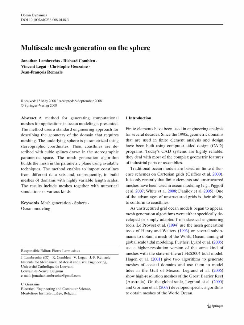
Let us consider a sphere S centered at the origin andof radius R, and one point s. This point lies on thesurface of the sphere, does no belong to the oceans,and will be the only singular point of the mapping. Asuitable choice for s could be a location in the mid-dle of Kazakhstan, but here, we choose s = {0, 0, −R}.It corresponds to the South Pole. Antarctica being acontinent, this choice makes sense for ocean modelingapplications. The stereographic projection consists inprojecting points p of the sphere on the plane z = R.

Beringstrait

Beringstrait

Antarctica

Antarctica

Fig. 2 Mesh of the World Ocean using the spherical coordinate system. The seam edge is visible on the right plot

Ocean Dynamics

Fig. 3 Stereographic projection

The stereographic projection u(x) = {u, v} of a pointx={x, y,z} is the intersection of vector q− p with z= R:

u = {u, v} ={

2RR + z

x,2R

R + zy}

,

x = {x, y, z} = 4R2

u2 + v2 + 4R2

{u, v, R

(4R2 − u2 + v2

)}.

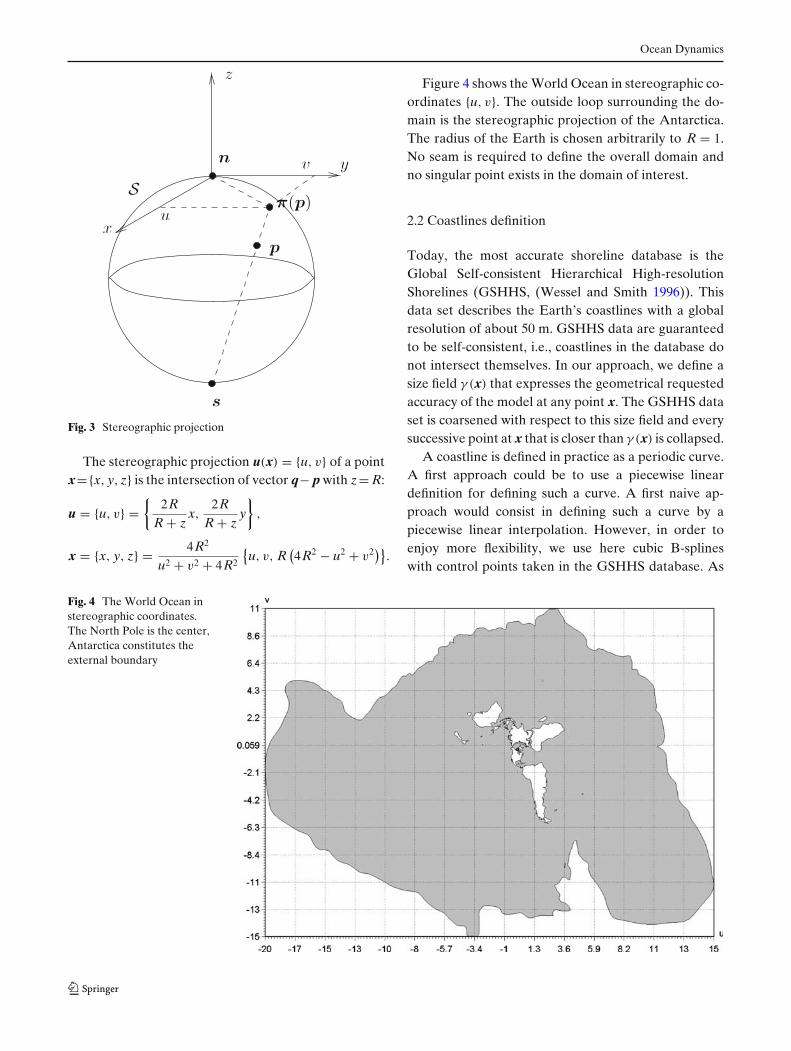
Figure 4 shows the World Ocean in stereographic co-ordinates {u, v}. The outside loop surrounding the do-main is the stereographic projection of the Antarctica.The radius of the Earth is chosen arbitrarily to R = 1.No seam is required to define the overall domain andno singular point exists in the domain of interest.

2.2 Coastlines definition

Today, the most accurate shoreline database is theGlobal Self-consistent Hierarchical High-resolutionShorelines (GSHHS, (Wessel and Smith 1996)). Thisdata set describes the Earth’s coastlines with a globalresolution of about 50 m. GSHHS data are guaranteedto be self-consistent, i.e., coastlines in the database donot intersect themselves. In our approach, we define asize field γ (x) that expresses the geometrical requestedaccuracy of the model at any point x. The GSHHS dataset is coarsened with respect to this size field and everysuccessive point at x that is closer than γ (x) is collapsed.

A coastline is defined in practice as a periodic curve.A first approach could be to use a piecewise lineardefinition for defining such a curve. A first naive ap-proach would consist in defining such a curve by apiecewise linear interpolation. However, in order toenjoy more flexibility, we use here cubic B-splineswith control points taken in the GSHHS database. As

Fig. 4 The World Ocean instereographic coordinates.The North Pole is the center,Antarctica constitutes theexternal boundary

Ocean Dynamics

Fig. 5 Great Britain andIreland with resolutions of100 km (top/left), 15 km(top/right), 1.5 km(bottom/left), and 150 m(bottom/right). Splinescontrol points are depicted onthe geometry with the twolowest resolutions

B-splines remain inside the convex hull defined by thecontrol points, it can be shown that, if the piecewiselinear representation is convex and consistent, then thecurvilinear B-splines representation is also consistent.

In Fig. 5, we generate the coastlines of Great Britainand Ireland with different resolutions. With a resolu-tion γ = 100 km, we only consider Ireland and GreatBritain, and we neglect all smaller islands. With a reso-lution of γ = 15 km, 15 contours appear in the domain.Typically, the Isle of Wight is now included. With a res-olution of γ = 1.5 km, the domain contains 152 islands.With a resolution of γ = 150 m, the domain contains2,176 islands and a total of 83,277 control points.

3 Mesh generation

As an accurate representation of the boundaries isnow available, the next task involves the generation offinite element meshes on curved surface. Two majorapproaches are available:

– Techniques for which the surface mesh is generateddirectly in the real 3D space

– Techniques for which the surface mesh is generatedin the parametric plane of the surface

When a parametrization of the surface exists, build-ing the mesh in the parametric plane appears to be themost robust choice.

3.1 Definition of a local mesh size field

The aim of the mesh generation process is to buildelements of controlled shape and size. Mesh generatorsare usually able to adapt to a so-called mesh size field.An isotropic mesh size field is a scalar function δ(x) thatdefines the optimal length of an edge at position x ofthe real space. In the domain of ocean modeling, thereexist some heuristics on the way mesh sizes should bedistributed in the World Ocean.

The mesh should take into account the bathymetry.The bathymetry H(x) is taken into account in twoways, leading to two fields f1 and f2. Gravity wavesmove at speed

√gH, with g being the acceleration of

gravity. The lengthscale λ of a gravity wave is thereforeproportional to λ = O(1/

√H). If we consider that N

mesh sizes are necessary to capture one wavelength,

Ocean Dynamics

and if λmin is the smallest wavelength that has to becaptured for a reference bathymetry Href , we definef1 as

f1(x) = λmin

N

√Href

H(x).

Another way of taking into account the bathymetryis to force the mesh to capture its variations with agiven accuracy (Gorman et al. 2006). Bathymetry canbe seen as a scalar field defined at mesh vertices andinterpolated piecewise linearly. As the first term oferror in its interpolation is supposed to depend onλmax, the greatest (in absolute value) eigenvalue of theHessian H(x),

H(x) = ∇∇(

H(x)

Href

),

we define the second field as:

f2(x) = 1√λmax

.

In order to represent coastlines well and to capturethe small-scale phenomena generated by the frictionon the coasts, mesh size should be even smaller nearcoastlines. This criterion has already been used in theliterature (e.g., Legrand et al. 2006). We define a firstfield f3(x) as the distance to the closest shoreline:

f3(x) = d(x).

This field f3 is also called a shore proximity function.This distance can be computed in place using the

Approximated Nearest Neighbor Algorithm (Aryaet al. 1998).

For each criterion field fi, a mesh size field δi iscomputed as follows:

δi(x) = δsmalli + αi(x)

(δ

largei − δsmall

i

),

where

αi(x) =

⎧⎪⎪⎪⎪⎨⎪⎪⎪⎪⎩

0 if fi(x) ≤ f mini

fi(x)− f mini

f maxi − f min

iif f min

i < fi(x) < f maxi

1 if fi(x) ≥ f maxi

with δlargei and δsmall

i as large and small desired meshsizes and f max

i and f mini as two field values that define

the zone of refinement. The final size field is simplycomputed as the minimum of all size fields:

δ(x) = min (δ1(x), δ2(x), . . . ).

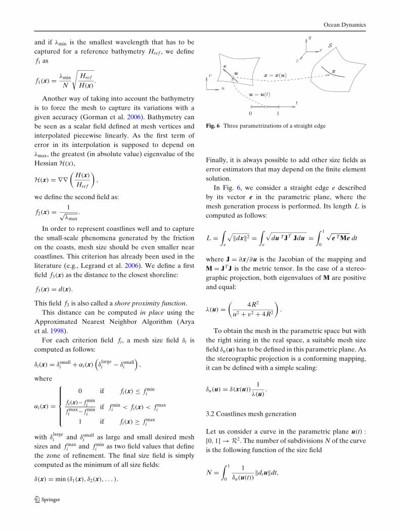
Fig. 6 Three parametrizations of a straight edge

Finally, it is always possible to add other size fields aserror estimators that may depend on the finite elementsolution.

In Fig. 6, we consider a straight edge e describedby its vector e in the parametric plane, where themesh generation process is performed. Its length L iscomputed as follows:

L =∫

e

√‖dx‖2 =

∫e

√du TJT Jdu =

∫ 1

0

√e TMe dt

where J = ∂x/∂u is the Jacobian of the mapping andM = JTJ is the metric tensor. In the case of a stereo-graphic projection, both eigenvalues of M are positiveand equal:

λ(u) =(

4R2

u2 + v2 + 4R2

).

To obtain the mesh in the parametric space but withthe right sizing in the real space, a suitable mesh sizefield δu(u) has to be defined in this parametric plane. Asthe stereographic projection is a conforming mapping,it can be defined with a simple scaling:

δu(u) = δ(x(u))1

λ(u).

3.2 Coastlines mesh generation

Let us consider a curve in the parametric plane u(t) :[0, 1] → R2. The number of subdivisions N of the curveis the following function of the size field

N =∫ 1

0

1

δu(u(t))‖dtu‖dt,

Ocean Dynamics

where ‖dtu‖ = √(∂tu)2 + (∂tv)2. The N + 1 mesh points

on the curve are located at coordinates {t0, . . . , tN}where ti is computed using the following rule:

i =∫ ti

t0

1

δu(u(t))‖dtc‖dt.

Integration of those expressions must be performedwith an adaptive trapeze rule, as coastlines are dis-cretized with cubic splines that contain a large numberof control points. Typically, Europe and Asia are dis-cretized by only one spline with more than 20 thousandcontrol points (Fig. 4).

However, this algorithm does not guarantee that,even if the model edges G1

j that constitute the bound-aries of the domain are nonintersecting, the corre-sponding 1D meshes do not self-intersect. Figure 7shows two islands very close to each other. Yet, even ifthe geometry is itself not self-intersecting, the first 1Dgenerated mesh intersects itself. This can be consideredas a critical issue: modifying the mesh size field by handlocally cannot be considered when several thousandislands are to be involved. It is therefore mandatoryto define a systematic recovery procedure. Such analgorithm, illustrated in Fig. 7, works as follows:

1. A Delaunay mesh that contains all points of the1D mesh is initially constructed using a divide-and-conquer algorithm (Dwyer 1986).

2. Missing edges are recovered using edge swaps(Weatherill 1990). If a mesh edge ei that belongs tothe 1D mesh is to be swapped for recovering edgee j, then the mesh edges ei and e j that both belongto the 1D mesh intersect.

3. All intersecting edges ek are split in two segmentsand the new point is snapped onto the geometry.Then, we go back to the first step until the list ofintersecting edges is empty.

If an intersecting edge is smaller than the geometricaltolerance, then an error message is thrown claimingthat the geometry is self-intersecting. Note that when aunique mesh edge connects two different islands, thoseislands are numerically merged if a nonslip boundarycondition is applied along their coastlines.

3.3 Surface mesh generation

To generate a mesh on the sphere, three approachesare available in Gmsh software. All of them start withan initial Delaunay mesh that contains all the mesh

Fig. 7 A geometry with two islands (in light and dark gray) thatare very close to each other. The top image shows the initial 1Dmesh that respects mesh size field. The middle image shows thefirst iteration of the recovery algorithm. The bottom image showsthe final mesh that was possible to realize after two recoveryiterations

vertices of the contours. Then, every mesh edge of the1D mesh is recovered using edge swaps. Then, internalvertices are iteratively inserted inside the domain.The way points are inserted differently in the threealgorithms:

– The del2d algorithm is inspired by the work ofthe GAMMA team at INRIA (George and Frey

Ocean Dynamics

2000). New points are inserted sequentially at thecircumcenter of the element that has the largestadimensional circumradius. The mesh is then re-connected using an anisotropic Delaunay criterion.

– In the frontal algorithm (Rebay 1993), new pointsare inserted optimally on Voronoï edges. The meshis then reconnected using the same anisotropicDelaunay criterion as the one in the del2d algo-rithm. Note that this algorithm’s implementationonly differs slightly from that of algorithm del2d.

– The meshadapt algorithm is very different from thefirst two ones. It is based on local mesh modifica-tion: This technique makes use of edge swaps, splits,and collapses. Long edges are split, short edgesare collapsed, and edges are swapped if a bettergeometrical configuration is obtained.

The frontal algorithm usually gives the highest-qualitymeshes while the del2d algorithm is the fastest: it pro-duces about five million triangles a minute if the sizefield δ is not too complex to compute. Figure 8 presentsthree meshes of one of the models of Fig. 5 for whichwe have used a shore proximity function as the onlysize field. Meshes have, respectively, 18,698, 19,514,and 17,154 triangles. The percentage of elements thathave an aspect ratio ρ > 0.9 is, respectively, 93.2%,88.1%, and 84.5%. CPU time for generating mesheswas, respectively, 0.7, 0.5, and 5.7 s.

Figures 9 and 10 present a mesh of the World Oceanthat makes use of all size fields defined in Section 3.1:

– A shore proximity function f1 is used with δsmall1 =

30 km, δlarge1 = 200 km, f min

1 = 0, and f max1 =

500 km.– We use f2 and refine the mesh proportionally to

the square root of the ocean depth. The size fieldδ2 ranges from 25 to 500 km.

– We use f3 to capture the bathymetry. The size fieldδ3 ranges from 25 to 500 km.

The resulting mesh is generated of 436,409 trianglesand the whole mesh generation process (data load-ing, coastline reduction, 1D mesh generation, 2D meshgeneration, output files writing) takes 35 s on a re-cent laptop. Those timings compare advantageously

a) Mesh done using the frontal algorithm

b) Mesh done using the del2d algorithm

c) Mesh done using the meshadapt algorithm

Fig. 8 Meshes of the same domain using three differentalgorithms (a–c)

Ocean Dynamics

Fig. 9 Mesh of the World Ocean. The mesh size field is definedusing a shore proximity function, the bathymetry, and its Hessian

with alternative techniques based on mesh decimation(Gorman et al. 2006). The memory footprint of themeshing algorithms is low: about 12 million triangles

(six million nodes) can be generated per gigabyte ofmemory.

4 Examples

In the mesh generation community, it is assumed thata good paper should present nice pictures of meshes.We will not circumvent that prerequisite. Yet, meshgeneration is usually considered as a tool, not as an aim.Therefore, the meshes that we present in this sectionare accompanied by some simulation results.

4.1 Sea ice modeling

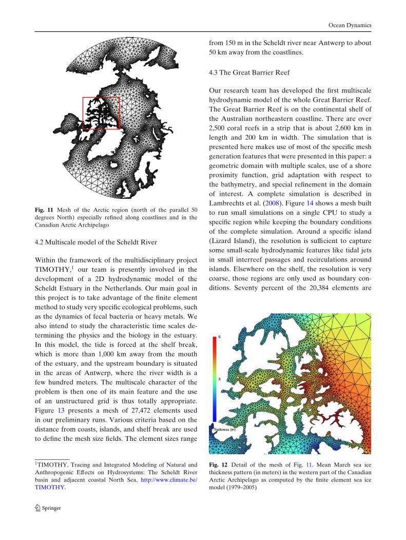
The mesh presented in Fig. 11 was used to investigatethe sensitivity of the Arctic sea ice cover features tothe resolution of the narrow straits constituting theCanadian Arctic Archipelago. This mesh constitutes of17,053 triangles with a resolution of 20 km near theislands in the archipelago and 40 km elsewhere. Farfrom coasts and islands, the resolution decreases up to300 km. Model results are shown in Fig. 12. A completedescription of the model and its validation can be foundin Lietaer et al. (2008).

Fig. 10 Close up of the meshof Fig. 9 in the north PacificOcean; color levels representthe bathymetry (in meters).The effects of the threerefinement rules are clearlyvisible

Ocean Dynamics

Fig. 11 Mesh of the Arctic region (north of the parallel 50degrees North) especially refined along coastlines and in theCanadian Arctic Archipelago

4.2 Multiscale model of the Scheldt River

Within the framework of the multidisciplinary projectTIMOTHY,1 our team is presently involved in thedevelopment of a 2D hydrodynamic model of theScheldt Estuary in the Netherlands. Our main goal inthis project is to take advantage of the finite elementmethod to study very specific ecological problems, suchas the dynamics of fecal bacteria or heavy metals. Wealso intend to study the characteristic time scales de-termining the physics and the biology in the estuary.In this model, the tide is forced at the shelf break,which is more than 1,000 km away from the mouthof the estuary, and the upstream boundary is situatedin the areas of Antwerp, where the river width is afew hundred meters. The multiscale character of theproblem is then one of its main feature and the useof an unstructured grid is thus totally appropriate.Figure 13 presents a mesh of 27,472 elements usedin our preliminary runs. Various criteria based on thedistance from coasts, islands, and shelf break are usedto define the mesh size fields. The element sizes range

1TIMOTHY, Tracing and Integrated Modeling of Natural andAnthropogenic Effects on Hydrosystems: The Scheldt Riverbasin and adjacent coastal North Sea, http://www.climate.be/TIMOTHY.

from 150 m in the Scheldt river near Antwerp to about50 km away from the coastlines.

4.3 The Great Barrier Reef

Our research team has developed the first multiscalehydrodynamic model of the whole Great Barrier Reef.The Great Barrier Reef is on the continental shelf ofthe Australian northeastern coastline. There are over2,500 coral reefs in a strip that is about 2,600 km inlength and 200 km in width. The simulation that ispresented here makes use of most of the specific meshgeneration features that were presented in this paper: ageometric domain with multiple scales, use of a shoreproximity function, grid adaptation with respect tothe bathymetry, and special refinement in the domainof interest. A complete simulation is described inLambrechts et al. (2008). Figure 14 shows a mesh builtto run small simulations on a single CPU to study aspecific region while keeping the boundary conditionsof the complete simulation. Around a specific island(Lizard Island), the resolution is sufficient to capturesome small-scale hydrodynamic features like tidal jetsin small interreef passages and recirculations aroundislands. Elsewhere on the shelf, the resolution is verycoarse, those regions are only used as boundary con-ditions. Seventy percent of the 20,384 elements are

Fig. 12 Detail of the mesh of Fig. 11. Mean March sea icethickness pattern (in meters) in the western part of the CanadianArctic Archipelago as computed by the finite element sea icemodel (1979–2005)

Ocean Dynamics

Fig. 13 Multiscale mesh:North Sea and Scheld RiverEstuary. Color levelsrepresent the amplitudeof the M2 tidal component(in meters)

located in the refined region. A plot of velocity vec-tors is also presented. Tidal jets and eddies due tothe interaction of the flow with the topography nearthe open-sea boundary are clearly visible. Those small-scale features were captured thanks to the accuratedescription of the bottom topography.

5 Summary

A CAD-based mesh generation procedure for oceanmodeling has been developed. The new approach hasthe advantage of relying on existing well-known engi-neering mesh generation procedures. The CAD model,based on a smooth BRep of the domain, allows tobuild a compact, self-consistent, and portable geomet-ric model. Existing robust meshing procedures can beapplied to the CAD model. Various meshes can be

constructed based on the same CAD definition, andvarious meshing algorithms can be used as well. Lastbut not least, everything that has been described inthis paper is now part of Gmsh, a 3D finite elementmesh generator with built-in pre- and postprocessingfacilities (http://www.geuz.org/gmsh). Since Gmsh isopen-source (under the GNU General Public License),anyone within the finite element marine modeling com-munity has the opportunity to use this freely.

Acknowledgements The present study was carried out withinthe scope of the project A second-generation model of theocean system, which is funded by the Communauté Française deBelgique, as Actions de Recherche Concertées, under contractARC 04/09-316. This work is a contribution to the SLIM2 project.

2SLIM, Second-generation Louvain-la-Neuve Ice-ocean Model,http://www.climate.be/SLIM

Ocean Dynamics

Lizard Island

Fig. 14 Coarse mesh of the Great Barrier Reef refined aroundLizard Island (top). Details of the simulation computed on thismesh in the vicinity of this island (bottom). Color levels show thedepth and the arrows indicate the bidimensional velocity field

References

Arya S, Mount DM, Netanyahu NS, Silverman R, Wu AY(1998) An optimal algorithm for approximate nearestneighbor searching. J ACM 45:891–923. http://www.cs.umd.edu/ mount/ANN/

Beall MW, Shephard MS (1997) A general topology-based meshdata structure. Int J Numer Methods Eng 40(9):1573–1596

Danilov S, Kivman G, Schröter J (2005) Evaluation of an eddy-permitting finite-element ocean model in the north atlantic.Ocean Model 10:35–49

Dwyer RA (1986) A simple divide-and-conquer algorithm forcomputing delaunay triangulations in o(n log log n) expectedtime. In: Proceedings of the second annual symposium oncomputational geometry, Yorktown Heights, 2–4 June 1986,pp 276–284

George P-L, Frey P (2000) Mesh generation. Hermes, LyonGorman G, Piggott M, Pain C (2007) Shoreline approxima-

tion for unstructured mesh generation. Comput Geosci 33:666–677

Gorman G, Piggott M, Pain C, de Oliveira R, Umpleby A,Goddard A (2006) Optimisation based bathymetry approx-imation through constrained unstructured mesh adaptivity.Ocean Model 12:436–452

Griffies SM, Böning C, Bryan FO, Chassignet EP, Gerdes R,Hasumi H, Hirst A, Treguier A-M, Webb D (2000) Devel-opments in ocean climate modeling. Ocean Model 2:123–192

Hagen SC, Westerink JJ, Kolar RL, Horstmann O (2001) Two-dimensional, unstructured mesh generation for tidal models.Int J Numer Methods Fluids 35:669–686 (printed version inRichard’s office)

Haimes R (2000) CAPRI: computational analysis programminginterface (a solid modeling based infra-structure for en-gineering analysis and design). Tech. rep., MassachusettsInstitute of Technology

Henry RF, Walters RA (1993) Geometrically based, automaticgenerator for irregular triangular networks. Commun Nu-mer Methods Eng 9:555–566

Lambrechts J, Hanert E, Deleersnijder E, Bernard P-E,Legat V, Wolanski J-FRE (2008) A high-resolution modelof the whole great barrier reef hydrodynamics. Estuar CoastShelf Sci 79(1):143–151. doi:10.1016/j.ecss.2008.03.016

Le Provost C, Genco ML, Lyard F (1994) Spectroscopy ofthe world ocean tides from a finite element hydrodynamicmodel. J Geophys Res 99:777–797

Legrand S, Deleersnijder E, Hanert E, Legat V, Wolanski E(2006) High-resolution, unstructured meshes for hydro-dynamic models of the Great Barrier Reef, Australia. EstuarCoast Shelf Sci 68:36–46

Legrand S, Legat V, Deleersnijder E (2000) Delaunay mesh gen-eration for an unstructured-grid ocean circulation model.Ocean Model 2:17–28

Lietaer O, Fichefet T, Legat V (2008) The effects of resolvingthe Canadian Arctic Archipelago in a finite element seaice model. Ocean Model 24:140–152. doi:10.1016/j.ocemod.2008.06.002

Lyard F, Lefevre F, Letellier T, Francis O (2006) Modelling theglobal ocean tides: modern insights from FES2004. OceanDyn 56:394–415

National Geographic Data Center (2006) ETOPO1 globalrelief model. http://www.ngdc.noaa.gov/mgg/global/global.html.

Piggott M, Gorman G, Pain C (2007) Multi-scale ocean mod-elling with adaptive unstructured grids. CLIVAR Exch

Ocean Dynamics

Ocean Model Dev Assess 12(42):21–23 (http://eprints.soton.ac.uk/47576/)

Rebay S (1993) Efficient unstructured mesh generation by meansof delaunay triangulation and Bowyer-Watson algorithm. JComput Phys 106:25–138

Weatherill NP (1990) The integrity of geometrical boundaries inthe two-dimensional delaunay triangulation. Commun ApplNumer Methods 6(2):101–109

Wessel P, Smith WHF (1996) A global self-consistent, hi-erarchical, high-resolution shoreline database. J GeophysRes 101(B4):8741–8743. http://www.soest.hawaii.edu/wessel/gshhs/gshhs.html

White L, Deleersnijder E, Legat V (2008) A three-dimensionalunstructured mesh finite element shallow-water model, withapplication to the flows around an island and in a wind-driven elongated basin. Ocean Model 22:26–47