Embed Size (px)
Citation preview
Multiscale Entropy and Its Implications to Critical Phenomena,Emergent Behaviors, and Information
Zi-Kui Liu1 • Bing Li2 • Henry Lin3
Submitted: 16 January 2019 / in revised form: 28 May 2019
� ASM International 2019
Abstract Thermodynamics of critical phenomena in a
system is well understood in terms of the divergence of
molar quantities with respect to potentials. However, the
prediction and the microscopic mechanisms of critical
points and the associated property anomaly remain elusive.
It is shown that while the critical point is typically con-
sidered to represent the limit of stability of a system when
the system is approached from a homogenous state to the
critical point, it can also be considered to represent the
convergence of several homogeneous subsystems to
become a macro-homogeneous system when the critical
point is approached from a macro-heterogeneous system.
Through the understanding of statistic characteristics of
entropy in different scales, it is demonstrated that the
statistic competition of key representative configurations
results in the divergence of molar quantities when
metastable configurations have higher entropy than the
stable configuration. Furthermore, the connection between
change of configurations and the change of information is
discussed, which provides a quantitative framework to
study complex, dissipative systems.
Keywords critical phenomena � entropy � information �invar � perovskites � second law of thermodynamics �statistic thermodynamics
1 Introduction
Thermodynamics is a science concerning the state of a
system described by a set of state variables. Entropy is one
of the state variables, representing the degree of disorder of
the system, i.e., the higher the disorder, the larger the
entropy.[1] While the first law of thermodynamics is on the
energy conservation, the second law of thermodynamics
dictates that any internal process (IP or ip) in a system must
produce entropy if it proceeds spontaneously and irre-
versibly. It should be noted though that the total entropy
change of the system also depends on how the system
exchanges entropy with the surroundings through heat and
mass and can be either positive or negative, and it is the
combined first and second laws of thermodynamics that
represents the over-all progress of the system. The degree
of order or disorder of a system may thus either increase or
decrease based on the external conditions and internal
processes, resulting in the change of the state of the system
in terms of internal configurations and their probabilities
that are denoted by the configurational entropy at the cor-
responding time and space scales.
Each of those configurations can be considered as a sub-
system itself with its own set of sub-configurations. For
This article is an invited paper selected from presentations at ‘‘PSDK
XIII: Phase Stability and Diffusion Kinetics,’’ held during MS&T’18,
October 14-18, 2018, in Columbus, Ohio. The special sessions were
dedicated to honor Dr. John Morral, recipient of the ASM
International 2018 J. Willard Gibbs Phase Equilibria Award ‘‘for
fundamental and applied research on topology of phase diagrams and
theory of phase equilibria resulting in major advances in the
calculation and interpretation of phase equilibria and diffusion.’’ It
has been expanded from the original presentation.
& Zi-Kui Liu
1 Department of Materials Science and Engineering, The
Pennsylvania State University, University Park, PA 16802
2 Department of Statistics, The Pennsylvania State University,
University Park, PA 16802
3 Department of Ecosystem Science and Management, The
Pennsylvania State University, University Park, PA 16802
123
J. Phase Equilib. Diffus.
https://doi.org/10.1007/s11669-019-00736-w

example, one can investigate the entropy of the universe
and a black hole,[2,3] a society,[4,5] an ecosystem,[6] a per-
son[7] or a compound,[8] and the entropy from the smaller
scale is homogenized and contributes to the entropy at the
larger scale. The present paper aims to discuss how the
homogenization of configurations can be formulated and
exchanged between scales in terms of configurational
entropies at different scales, its probability at neighboring
scale and its application to systems with critical points.
Additionally, the entropy production of an internal process
is correlated with the generation and erasure of information
and reflects the information stored in the system in terms of
multiscale configurations. It is noted that the present work
is closely related to the renormalization theories[9,10] with
the system at one scale consisting of self-similar copies of
itself when viewed at another scale, and the different
parameters at various scales are used to describe the con-
stituents of the system. It is shown in the present work that
the entropy and statistical probability of each configuration
are the parameters that connect the scales.
2 Review of Fundamentals of Entropy
In thermodynamics, the entropy change of a system, dS,
can be written as follows[11,12]
dS ¼ dQ
TþX
SidNi þ dipS ðEq 1Þ
where dQ and dNi are the heat and the amount of com-
ponent i that the system receives from or release to the
surroundings, T is the temperature, Si is the molar entropy
of component i in the surroundings for dNi[ 0 or the
system for dNi\ 0, often called partial entropy of com-
ponent i, and dipS is the entropy production due to inde-
pendent IPs with each that may contain a group of coupled
processes. It is evident that the first two terms concern the
interactions between the surroundings and the system,
while the third term embodies what happens inside the
system. Equation 1 thus establishes a bridge connecting the
interior of a system in terms of internal entropy production
and the exterior of the system in terms mass and heat
exchanges.
Combining Eq 1 with the first law of thermodynamics,
the combined law of thermodynamics can be obtained.
While the work exchanges between the system and sur-
rounding can involve mechanical, electric, and magnetic
works, it is often that the work due to hydrostatic pressure
is considered,[11,12] and the combined law of thermody-
namics is written as follows
dU ¼ TdS� PdV þX
lidNi � TdipS
¼X
YadXa � TdipS ðEq 2Þ
where T, P and V are temperature, pressure, and volume,
respectively, and li is the chemical potential of component
i. In the second part of Eq 2, Ya denotes the potentials, i.e.,
T, - P and li, and Xa denotes the molar quantities, i.e., S,
V and Ni.[11,12] It should be emphasized that both dV and
dNi in Eq 2 refer to the changes between the system and
surroundings, while dS contains the contributions from IPs
as shown by Eq 1.
By introducing the driving force for each independent
IP, j, the energy change due to the entropy production can
be represented by the product of driving force for the IP,
Dip;j, and the change of corresponding internal variable,
dnj, in terms of the Taylor expansion up to the third order
as follows[11]
TdipS ¼X
Dip;jdnj �1
2
XDip;jkdnjdnk
þ 1
6
XDip;jkldnjdnkdnl ðEq 3Þ
where the second and third terms are added for discussion
of stability of the system based on their signs when the first
summation in the equation equals zero, i.e. the system is at
a state of equilibrium.[13]
The second law of thermodynamics requires that each
independent IP, if proceeding spontaneously, must have a
positive entropy production, i.e. Dip;j [ 0 to give
TdipS[ 0. Consequently, the system reaches a state of
equilibrium when Dip;j � 0 for all IPs. This equilibrium
state is stable with respect to fluctuations of internal vari-
ables when Dip;jk [ 0 due to the negative entropy produc-
tion and unstable when Dip;jk\0 due to the positive entropy
production for the IP of interest, both as shown by Eq 3.
When Dip;jk ¼ 0 the system is at the limit of stability. The
limit of stability becomes a critical point in the space of
independent internal variables njnknl with additional
Dip;jkl ¼ 0. The critical point in the space of all possible
independent internal variables of the system is termed as
the invariant critical point (ICP).[14] For a homogeneous
system, the IPs involve the movement of molar quantities
inside the system, and one can write the stability variables
of one IP as follows[11]
Dip;XaXa ¼ o2U
o Xað Þ2
" #
Xb
¼ oYa
oXa
� �
Xb
ðEq 4Þ
Dip;XaXaXa ¼ o3U
o Xað Þ3
" #
Xb
¼ o2Ya
o Xað Þ2
" #
Xb
ðEq 5Þ
For heterogeneous systems with chemical reactions, the
IPs are more complicated and may or may not be explicitly
spelled out.[15]
Equation 1 concerns the change of entropy. To obtain
the absolute value of entropy, one can integrate the
J. Phase Equilib. Diffus.
123
equation under the condition of reversible addition of heat
to the system in equilibrium with dNi ¼ 0 and dipS ¼ 0, i.e.
S ¼ S0 þ rT0
CdT
TðEq 6Þ
where S0 is the entropy at zero Kelvin, conventionally
assigned to be zero in terms of the third law of thermo-
dynamics, and C the heat capacity of the system, denoting
the heat needed to increase the temperature of the system
by one degree.
3 Statistics of Entropy
The discussion in the previous section has not concerned
the statistic characteristics of entropy. Gibbs[16] pointed out
that the entropy is defined as the average value of the
logarithm of probability of phase where the differences in
phases are with respect to configuration. Therefore, the
configurational entropy in a system of interest with prop-
erly defined time and space scales can be written as
Sconf ¼ �kBXm
k¼1
pk ln pk ðEq 7Þ
where kB is the Boltzmann constant, and pk the probability
of configuration k 2 1; . . .;mf g of the system withPmk¼1 p
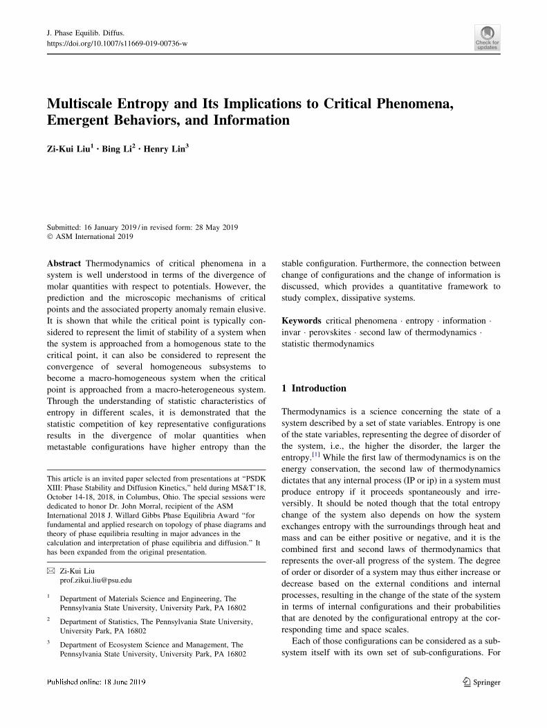
k ¼ 1 as shown in the upper row of Fig. 1(a). Since
each configuration k has its own entropy, Sk, the total
entropy of the system can be written as
S ¼Xm
k¼1
pkSk þ Sconf ¼Xm
k¼1
pk Sk � kB ln pk
� �ðEq 8Þ
Equations 6 and 8 should give the same entropy value
when they are counted on the same time and space scales.
By the same token, the configuration k is composed of
configurations in the scale of short time and smaller
dimension and can be written as
Sk ¼Xn
l¼1
pljk Sljk � kB ln pljk
� �ðEq 9Þ
where pljk and Sljk are the conditional probability and
entropy of configuration l 2 1; . . .; nf g as sub-configura-
tions of configuration k withPn
l¼1
pljk ¼ 1 as shown in the
lower row of Fig. 1(a). Equation 8 can then be re-orga-
nized as follows
S ¼Xm
k¼1
pkXn
l¼1
pljk Sljk � kB ln pljk
� �� kB ln p
k
!
ðEq 10Þ
This equation can be extended in the directions of larger
and smaller dimensions to capture more complexity of the
system or in the directions of longer and shorter time to
capture evolution of the system. The examples of config-
urations k 2 1; . . .;mf g and l 2 1; . . .; nf g are the magnetic
spin and vibrational configurations for cerium and Fe3Pt,
and the atomic and vibrational configurations for the mis-
cibility gap in the fcc Al-Zn solution, respectively, dis-
cussed in section 6.
On the other hand, from a statistics point of view, one
can calculate the direct contributions from the configura-
tions in the scale l to the system as follows by re-organizing
Eq 10 with the joint probability defined as pk;l ¼ pkpljk,
S ¼Xm
k¼1
Xn
l¼1
pkpljk Sljk � kB ln pkpljk� �� �
¼Xm
k¼1
Xn
l¼1
pk;l Sljk � kB ln pk;l
� �ðEq 11Þ
It is self-evident that Eq 11 is the same as the combi-
nation of Eq 8 and 9 due toPn
l¼1 pljk ¼ 1 andPn
l¼1 pljkkB ln pk
� �¼ kB ln p
k. Furthermore, one may
attempt to switch the order of summation of k and l, i.e.,
S ¼Xn
l¼1
Xm
k¼1
pk;lSljk
!� kB
Xm
k¼1
pk;l ln pk;l
" #ðEq 12Þ
This is analogue to Eq 10, but with the configuration
l 2 1; . . .; nf g with sub-configuration of k 2 1; . . .;mf g as
shown in Fig. 1(b). As proved below, the two scenarios in
Fig. 1(a) and (b) indeed give the same entropy of the
system.
Let us define the following
ql ¼Xm
k¼1
pkpljk ðEq 13Þ
Fig. 1 Two scenarios of configurations of a system, (a) k 21; . . .;mf g configurations with each of them composed of l 21; . . .; nf g sub-configurations; (b) l 2 1; . . .; nf g configurations with
each being the statistic average of each l 2 1; . . .; nf g sub-configu-
ration in all k 2 1; . . .;mf g configurations
J. Phase Equilib. Diffus.
123

qkjl ¼ pkpljkPmk¼1 p
kpljk¼ pkpljk
ql¼ pk;l
qlðEq 14Þ
Tl ¼Xm
k¼1
qkjl Sljk � kB ln qkjl
� �ðEq 15Þ
wherePn
l¼1 ql ¼ 1,
Pmk¼1 q
kjl ¼ 1, Tl is the entropy of a
configuration in l 2 1; . . .; nf g with sub-configuration of
k 2 1; . . .;mf g (see Fig. 1b), and Eq 14 the commonly
referred Bayes’s theorem.[17] It can be seen that Tl consists
of two parts: a) the entropy of each configuration in the
lower row of Fig. 1(b), i.e.Pm
k¼1 qkjlSljk which is evaluated
from the entropy of each configuration in l 2 1; . . .; nf g for
all configurations in k 2 1; . . .;mf g, and b) the configura-
tion among them, i.e. �kBPm
k¼1 qkjl ln qkjl.
The proof for the fact that the two scenarios schemati-
cally depicted in Fig. 1(a) and (b) have the same entropy is
as follows.
Theorem If
S ¼Xm
k¼1
pk Sk � kB ln pk
� �ðEq 16Þ
then
S ¼Xn
l¼1
ql Tl � kB ln ql
� �ðEq 17Þ
Proof From Eq 11 or 12 and using Eq 13 to 15
S ¼Xn
l¼1
Xm
k¼1
pk;l Sljk � kB ln pk;l
� �
¼Xn
l¼1
Xm
k¼1
qlqkjl Sljk � kB ln qlqkjl
� �
¼Xn
l¼1
qlXm
k¼1
qkjl Sljk � kB ln qlqkjl
� �( )
¼Xn
l¼1
qlXm
k¼1
qkjl Sljk � kB ln qkjl
� �" #� kB ln q
lXm
k¼1
qkjl
( )
¼Xn
l¼1
ql Tl � kB ln ql
� �
ðEq 18Þ
This proof is important as it demonstrates that the
sequence of configuration averaging can be switched in
terms of their scales, i.e. either at the scale k 2 1; . . .;mf gor l 2 1; . . .; nf g with the other scale as its sub-configura-
tions as schematically depicted in Fig. 1(a) and (b). Pro-
vided individual and joint probabilities of configurations in
the system can be evaluated, the entropy of the system
remains invariant independent of the scale where the
statistic averaging is carried out. The implications of this
conclusion will be further discussed in section 6.
4 Probability of Configurations
Probability of individual configurations of a system at
given time and space scales can be evaluated when their
energetics are known at the corresponding time and space
scales through their partition functions. For a closed system
under constant temperature and volume, a collection of
possible configurations of the system comprises a canonical
ensemble. In the discrete form, the canonical partition
function is defined as follows[18]
Z ¼X
k
Zk ¼X
k
e� Fk
kBT ðEq 19Þ
where Zk and Fk are the partition function and Helmholtz
energy of configuration k with
Fk ¼ �kBT ln Zk ðEq 20Þ
It should be mentioned that in the literature, the internal
or total energy, Uk, is often used in the place of Fk, which
implicitly assumes that the entropy of each configuration is
negligible. This assumption is not valid at high tempera-
tures as the individual configurations can have different
entropy values resulting in significant change of their
respective probabilities. It is noted that Asta et al.[19] used
an equation similar to Eq 19 for systems under constant
temperature, pressure, and chemical potentials.
The probability of each configuration can be defined as
pk ¼ Zk
Z¼ e
F�Fk
kBT ðEq 21Þ
where F is the Helmholtz energy of the system and can be
written as follows[8,20]
F ¼ �kBT ln Z ¼X
k
pkFk þ kBTX
k
pk ln pk ðEq 22Þ
It can be seen that the configurational entropy by Eq 7 is
shown in the last term in Eq 22, and from Eq 21 that
F�Fk for pk � 1, originated fromP
k pk ln pk � 0. The
equality holds when the system has only one configuration.
The above discussion does not consider interactions
between configurations. However, when the fluctuation
dimension is smaller than the dimension of the system,
there are interactions between configurations that may
result in new configurations that are not part of the existing
configurations. These interactions may be considered
explicitly by adding interaction terms in Eq 22 similar to
the CALPHAD modeling method in thermodynamics in the
form of p jpkLjk with Ljk being the interaction
J. Phase Equilib. Diffus.
123

energy.[11,21,22] On the other hand, a better approach is to
expand the set of configurations to include the new con-
figurations with the statistic approach intact as discussed in
this paper.
Furthermore, experimental measurements can only
detect the combined effect from all configurations. For the
properties of individual configurations, one has to rely on
theoretic calculations. The first-principles quantum
mechanics technique based on the density functional theory
(DFT)[23] along with the sophisticated computer pro-
grams[24,25] and ubiquitous high performance comput-
ers[26,27] have enabled the quantitative predictions of
ground states of a vast configurations as reflected in a
number of online databases.[28–30] The Helmholtz energy
of a configuration can be effectively evaluated from either
phonon calculations[31,32] or the Debye model[33] with the
scaling factor obtained from the elastic properties[34] pre-
dicted from first-principles calculations.[35–37] For config-
urations with disordering, the cluster expansion
approach[38,39] or the special quasirandom structures
(SQS)[40–42] can be used. It is also possible to sample
configurations at finite temperatures through the ab initio
molecular dynamics (AIMD) calculations[43] with the
atomic forces computed on the fly using the DFT-based
first-principles calculations as recently demonstrated for
PbTiO3 that are discussed in more detail in section 7.[44,45]
5 Thermodynamics of Critical Phenomena
Thermodynamics of critical phenomena is usually dis-
cussed in terms of the instability of a homogeneous system
derived from the combined law, i.e. Eq 2, as Eq 4 and
follows[11]
oYa
oXa¼ 0 ðEq 23Þ
The thermodynamic criterion of instability based on
entropy is written as
oT
oS¼ 0 ðEq 24Þ
When the system approaches the limit of stability,[11]
this derivative approaches zero, and its inverse, i.e., the
change of the entropy of the system, diverges, i.e.
oS
oT¼ þ1 ðEq 25Þ
The fluctuation of configurations reaches the whole
system. After crossing the limit of stability, the system
becomes inhomogeneous in the time and space scales
under consideration.
Differentiation of Eq 8 with respect to temperature gives
oS
oT¼X
k
opk
oTSk � kB ln p
k� �
þ pkoSk
oT� kB
pkopk
oT
� � �
¼ oSN
oT
þX
k 6¼N
opk
oTSk � SN � kB ln
pk
pN
� þ pk
oSk
oT� oSN
oT
� � �
ðEq 26Þ
where N denotes the configuration with the lowest Helm-
holtz energy, i.e., the ground state at zero Kelvin, andP
k pk ¼ 1 and
Pkopk
oT¼ 0 are used. In Eq 26, oSN
oTis posi-
tive from Eq 4, and the summation in Eq 26 would also be
positive if Sk [ SN that results in the increase of pk from
zero at zero Kelvin at the expense of pN .
Differentiation of Eq 21 yields
opk
oT¼ pk
kBT2Fk � F� �
þ T Sk � S� � �
¼pk Sk � S� �
kBT1þ Fk � F
T Sk � Sð Þ
� �ðEq 27Þ
Equation 27 further demonstrates that opk
oT[ 0 due to
Sk [ S with S � SN at the limit of pk near zero and Fk [F.
It is evident that a dramatic increase of oSoT
has to come from
the dramatic increase of opk
oT, i.e., the significant competition
between the metastable configurations k ¼ 1. . .N � 1ð Þand the ground state configuration (N) with Fk [FN . This
means rapid change rate of some F�Fk
kBTin some temperature
ranges with respect to the limit of stability.
Therefore, the thermodynamic criterion for instability
and critical phenomena is that the entropies of
metastable configurations are higher than that of the
stable configuration, but their differences are large enough
that the stable configuration remains stable with respect to
the metastable configurations so that there are no first-order
transitions until the instability and critical point are
reached.
6 Examples: Anti-Invar Cerium, Invar Fe3Pt,and Al-Zn binary
Cerium (Ce) is a unique element. Its ground state config-
uration under ambient pressure is non-magnetic face cen-
tered cubic (fcc) and its stable configuration at room
temperature is ferromagnetic fcc with some degree of
magnetic disordering, while all other magnetic elements in
the chemical periodic table are opposite with their ground
state configuration being magnetic. Ce has a critical point
around TC = 480-600 K and PC = 1.45-2 GPa with the
upper bound commonly accepted in the literature with
details discussed in Ref. 46.
J. Phase Equilib. Diffus.
123

In an effort to predict the thermodynamic properties of
Ce, we first considered two configurations: non-magnetic
(NM) and ferromagnetic (FM) with their Helmholtz ener-
gies predicted by first-principles calculations using the
partition function approach discussed above.[46] It should
be noted that the entropy in the Helmholtz energy of each
individual configuration contains the configurational con-
tributions from lower scales, i.e. thermal electronic con-
figurational contributions due to non-zero electronic
density at the Fermi level and the vibrational frequency
configurational contributions due to atomic vibrations as
shown below[32]
Fk ¼ Ec þ Fvib þ Fel ðEq 28Þ
where Ec is the static total energy at 0 K predicted by first-
principles calculations, Fvib the lattice vibrational free
energy, and Fel the thermal electronic contribution. The
first term can be calculated directly using e.g. VASP
code.[47] Fvib and Fel are related to contributions at finite
temperatures with the same equation form as Eq 7. Fel,
which is evaluated from the electronic densities of state at
different volumes,[32] is important for metals due to the
non-zero electronic density at the Fermi level. Fvib can be
obtained from first-principles phonon calculations for
accurate results[32,33] or the Debye model for the sake of
simplicity using the modified scaling factor.[34]
However, the consideration of two configurations was
not able to reproduce the experimentally observed critical
phenomena. This is because their fluctuations in the finite
space result in the interactions of magnetic spins in dif-
ferent orientations which are not captured by the two
configurations considered. Following the conventional
approach in the literature, an additional contribution to the
free energy of the system in terms of ‘local-moment’
mechanism was added to account for the magnetic spin
disordering, resulting in good agreement with experimental
observations as shown in Fig. 2 for total entropy and T–V
phase diagram along with all other anomalies in the system
as detailed in Ref. 46 such as the critical point at TC ¼476K and PC ¼ 2:22GPa.
The next step is to add an antiferromagnetic (AFM)
configuration. The first-principles calculations predict that
the static energy of the AFM configuration is between
those of NM and FM configurations.[48] Since the inter-
action due to magnetic spin disordering is included in the
AFM configuration, the ‘local-moment’ mechanism was
no-longer needed. The fluctuation of the NM, AFM, and
FM configurations enabled the predictions of all anomalies
in the system as shown in Fig. 3 for various entropy
changes and T-P phase diagram in addition to Schottky
anomaly for heat capacity. Particularly the overestimated
entropy change of the transition along the phase boundary
in our previous work with two configurations only and the
‘local-moment’ mechanism[46] was corrected, and the
critical point was predicted at TC ¼ 546K and
PC ¼ 2:05GPa, closer to the commonly accepted values
than our previous predictions. The key is that the interac-
tions between two configurations when they fluctuate is
included in the thrid configuration.
The underlying physics of our ‘itinerant-electron’
magnetism model[48] closely resembles the Kondo-Ander-
son magnetic model as summarized by Kouwenhoven and
Glazman.[49] At low temperatures, the Kondo-Anderson
model states that impurity magnetic moment and one
conduction electron moment bind and form an overall
nonmagnetic configuration, while at high temperatures, the
binding is broken resulting in a magnetic entropy of
approximately kB ln 2. In our itinerant-magnetism model
for the Ce transition, the nonmagnetic is the occupied
Fig. 2 (a) Total entropy, S, and vibrational entropy change, DSvib, ofCe at 0 GPa with T (K) and (b) T–V phase diagram of Ce, with details
in Ref. 46
J. Phase Equilib. Diffus.
123

ground configuration and the magnetic configurations are
empty at 0 K. At finite temperatures, our model has a
magnetic entropy term as shown by Eq 7, slightly different
from the simple Kondo-Anderson model. At high enough
temperatures the mixture between the FM and AFM con-
figurations results in a magnetic entropy of � kB ln 2 as
shown by the populations of configurations in Fig. 4.
It should be noted that the changes of all physical
properties diverge at the critical point as shown by Eq 25.
For example, Fig. 5(a) plots the predicted T–V phase dia-
gram of Ce with isobaric volume curves and available
experimental data superimposed. It can be seen that oVoT
)þ1 at the critical point marked by the green circle, and
significant anomaly exists at pressures considerably away
from the pressure at the critical point. Since V and T are not
conjugate variables in the combined law of thermody-
namics (see Eq 2),[11] the positive sign of oVoT
is not
thermodynamically guaranteed. It depends on the volumes
of the metastable configurations.[50,51]
For example, the isobaric volume curves in the T–V
phase diagram of Invar Fe3Pt in Fig. 5(b) show oVoT
) �1at the critical point marked by the green circle and oV
oT\0 in
a considerable temperature ranges away from the critical
point. In this system, a supercell with 9 Fe and 3 Pt atoms
was considered, resulting in 29=512 magnetic configura-
tions with 37 of them being unique due to the symmetry.
This negative thermal expansion or thermal contraction is
because the metastable magnetic spin-flip configurations
have smaller molar volumes than the FM configuration in
Fe3Pt. When the probability of the metastable magnetic
spin-flip configurations increases with temperature due to
their higher entropies than that of the FM configuration, the
thermal expansion of the system, i.e. oVoT, is the result of the
competition between the positive thermal expansion of
each configuration and the volume reduction due to the
replacement of the FM configuration by the magnetic spin-
flip configurations. When the latter is larger than the for-
mer, the thermal expansion of the system becomes nega-
tive. These anomalies can be generalized to a wide range of
emergent behaviors for all physical properties of a system,
when a system exhibits properties that its constituents do
not possess such as negative thermal expansion in Fe3Pt
discussed above, with respect to composition and elastic,
electric, magnetic fields, and their combinations with the
present model as the theoretical foundation.[14,44,45,51]
In both Ce and Fe3Pt cases, the configurations in the
k 2 1; . . .;mf g scale are various magnetic configurations
with two sets of sub-configurations, i.e. thermal electronic
and vibrational configurations, in the l1 2 1; . . .; n1f g and
l2 2 1; . . .; n2f g scales. Based on the discussions in sec-
tion 3, it is possible to construct two new sets of thermal
electronic and vibrational configurations averaged across
Fig. 3 (a) Predicted entropy changes in terms of lattice vibration
(lat), lattice vibration plus thermal electron (lat ? el), and lattice
vibration plus thermal electron and plus configuration coupling
(lat ? el ? f) changes along the phase boundary, (b) Predicted T–P
phase diagram, both in comparison with experimental data with
details in Ref. 48
Fig. 4 Thermal populations, i.e. pk, of the nonmagnetic (red dot-
dashed), anti-ferromagnetic (green dashed), and ferromagnetic (blue
solid) as a function of temperature at the critical pressure of 2.05 GPa
from Ref. 48
J. Phase Equilib. Diffus.
123

various magnetic configurations so that the thermal elec-
tronic and vibrational properties of the system can be
predicted. The corresponding results are being investigated
and will be published separately.
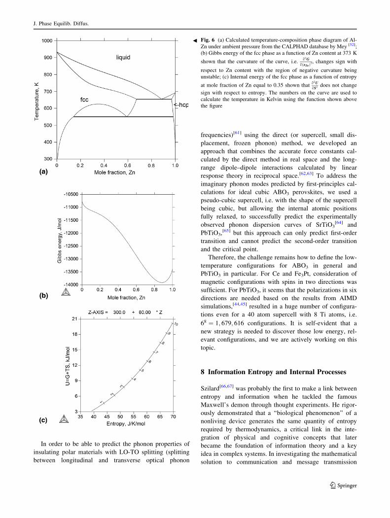
Let us consider the Al-Zn binary system with its phase
diagram under ambient pressure shown in Fig. 6(a) calcu-
lated from the CALPHAD database in the literature[52] with
a miscibility gap in the fcc phase. When the Gibbs energy
is plotted with respect to the composition of Zn in
Fig. 6(b), its curvature, i.e. the chemical potential deriva-
tive with respect to composition, changes sign in accor-
dance with the stability criterion that the derivative of a
potential with respect to its conjugate molar quantity
changes sign at the limit of stability.[11] However, the plot
of the internal energy with respect to entropy in
Fig. 6(c) does not change its curvature as it should when
crossing the stability boundary based on Eq 24. This
indicates that the present CALPHAD modeling of critical
phenomena needs to be further improved with multiple
configurations as discussed above.[45]
7 Unresolved Issues in ABO3 Perovskites
ABO3 perovskites represent a group of ferroelectric
materials that directly convert electrical energy to
mechanical energy or vice versa. Many of them experience
ferroelectric-paraelectric (FE-PE) phase transitions as a
function of temperature or electric field. As an insulator,
lead titanate (PbTiO3, PTO) is a benchmark ferroelectric
material. The phase transition between its two known
perovskite structures, i.e. the ferroelectric tetragonal phase
and the para-electric cubic phase,[53] occurs at about 763 K
at ambient pressure and at room temperature at about
12 GPa[54,55] and has been considered as a classical
example to understand structural and ferroelectric phase
transitions in perovskites.[44,54,56–58]
The ferroelectricity in the tetragonal PbTiO3 phase is due
to the displacement of Ti atoms away from the center position
in the tetragonal structure, resulted in spontaneous electric
polarization. While the FE-PE phase transition is regarded as
the typical displacive transition associated with softening of
the relevant phononmodes, a certain degree of order–disorder
mechanism has been considered in the literature associated
with the orientation change of local distortions.[59,60] The
direct calculation of the free energy of the para-electric cubic
PbTiO3 phase in terms of Eq 28 is not possible because its
vibrational free energy cannot be evaluated due to its insta-
bility at zeroK and ambient pressure. On the other hand, x-ray
absorption fine-structure (XAFS) measurements by Sicron
et al.[59] showed that the Ti atoms are displaced relative to the
oxygen octahedra cage center both below and above the FE-
PE phase transition temperature.
Through AIMD simulations shown in Fig. 7, Fang
et al.[44] observed that the amount of tetragonal configu-
ration decreases with the increase of temperature and
reaches a plateau slightly below 50% above the FE-PE
transition temperature in the cubic PbTiO3 phase region
with this transition temperature defined by the x-ray
diffractions with lower time and spatial resolutions than
those of XAFS (Fig. 7a).[54] Figure 7(b) also shows that
about 80% of the tetragonal configurations in the cubic
phase region are polarized though the over-all polarization
is almost zero.[44] The other half of the Ti atoms in the
cubic configuration are on transition from one to another
polarization directions at any moment of time.[45] This
observation confirms our theory as discussed in the previ-
ous section for Invar Fe3Pt and anti-Invar Ce, i.e. high-
temperature structures are dynamic averages of low-tem-
perature configurations.
Fig. 5 Predicted temperature–volume phase diagrams with the
miscibility gap (yellow shaded area) and critical point (green circle)
marked,[8] (a) cerium and (b) Fe3P. Additional isobaric volumes are
plotted for several pressures with available experimental data
superimposed
J. Phase Equilib. Diffus.
123
In order to be able to predict the phonon properties of
insulating polar materials with LO-TO splitting (splitting
between longitudinal and transverse optical phonon
frequencies)[61] using the direct (or supercell, small dis-
placement, frozen phonon) method, we developed an
approach that combines the accurate force constants cal-
culated by the direct method in real space and the long-
range dipole–dipole interactions calculated by linear
response theory in reciprocal space.[62,63] To address the
imaginary phonon modes predicted by first-principles cal-
culations for ideal cubic ABO3 perovskites, we used a
pseudo-cubic supercell, i.e. with the shape of the supercell
being cubic, but allowing the internal atomic positions
fully relaxed, to successfully predict the experimentally
observed phonon dispersion curves of SrTiO3[64] and
PbTiO3,[65] but this approach can only predict first-order
transition and cannot predict the second-order transition
and the critical point.
Therefore, the challenge remains how to define the low-
temperature configurations for ABO3 in general and
PbTiO3 in particular. For Ce and Fe3Pt, consideration of
magnetic configurations with spins in two directions was
sufficient. For PbTiO3, it seems that the polarizations in six
directions are needed based on the results from AIMD
simulations,[44,45] resulted in a huge number of configura-
tions even for a 40 atom supercell with 8 Ti atoms, i.e.
68 ¼ 1; 679; 616 configurations. It is self-evident that a
new strategy is needed to discover those low energy, rel-
evant configurations, and we are actively working on this
topic.
8 Information Entropy and Internal Processes
Szilard[66,67] was probably the first to make a link between
entropy and information when he tackled the famous
Maxwell’s demon through thought experiments. He rigor-
ously demonstrated that a ‘‘biological phenomenon’’ of a
nonliving device generates the same quantity of entropy
required by thermodynamics, a critical link in the inte-
gration of physical and cognitive concepts that later
became the foundation of information theory and a key
idea in complex systems. In investigating the mathematical
solution to communication and message transmission
Fig. 6 (a) Calculated temperature-composition phase diagram of Al-
Zn under ambient pressure from the CALPHAD database by Mey [52];
(b) Gibbs energy of the fcc phase as a function of Zn content at 373 K
shown that the curvature of the curve, i.e.o2G
o xZnð Þ2, changes sign with
respect to Zn content with the region of negative curvature being
unstable; (c) Internal energy of the fcc phase as a function of entropy
at mole fraction of Zn equal to 0.35 shown thato2U
oS2does not change
sign with respect to entropy. The numbers on the curve are used to
calculate the temperature in Kelvin using the function shown above
the figure
b
J. Phase Equilib. Diffus.
123

problems, Shannon[4,68] proposed the concept of informa-
tion entropy as the measure of the amount of information
that is missing before reception or before communication is
achieved and defined the information entropy as a macro-
state (a source) with the number of possible microstates
(ensembles of possible messages) that could be sent by that
source. Thus, information in the communication begins
with a set of messages, each with a probability, and the
average information content per message is defined in
analogy with Eq 7.
Brillouin extensively studied the relations between
thermodynamics and information and suggested that
information can be quantified using a system’s
entropy.[69–73] He noted that entropy itself measures the
lack of information about the actual structure of a system
and proposed that information corresponds to a negative
term in the final entropy of a physical system as follows[70]
Sfinal ¼ Sinitial � I ðEq 29Þ
where Sinitial and Sfinal are the initial and final entropies of
the system, and I the information of the system. Brillouin’s
idea of dealing with information and physical entropy on
an equal basis has been widely accepted in the commu-
nity.[74] The exchange between energy and information
was further elaborated by Landauer[75,76] who perceived
that a logically irreversible process reduces the degrees of
freedom of the system, thus entropy, and therefore must
dissipate energy into the environment, hence erasing
information in memory entails entropy increase in the
environment. This is commonly referred to as Landauer’s
erasure principle, also investigated theoretically by Ben-
nett[77] and more recently verified experimentally.[78,79]
Let us use the IP discussed in the present paper to
understand the concept of information and its generation or
loss. This IP may consume some masses/nutrients dNni
� �,
generate some output masses/wastes dNwj
� �and heat
dipQ� �
, and re-organize its configurations to produce cer-
tain amount of information dipI� �
, resulting in the entropy
production with a similar form as Eq 1
dipS ¼ dipQ
T�X
Sni dNni þ
XSwj dN
wj � dipI ðEq 30Þ
where Sni and Swj are the entropies of nutrient i and waste j,
respectively. Let us study several thought experiments of
spontaneous IP, i.e. dipS[ 0:
a. dNni ¼ dNw
j ¼ 0, the IP behaves like a closed system
(i.e., involving no nutrient consumption and no waste
generation)
a:1. dipI[ 0, the IP produces more information,
and the sub-system must have
dipQ[ TdipI[ 0, i.e. the IP must generate
heat to be dissipated out to its surroundings, in
accordance with the Landauer’s erasure prin-
ciple. The more information is reflected by the
more distinct configurations, such as formation
of crystal from its liquid and data
writing;[68,80–82]
a:2. dipI\0, with information loss and
dipQ[ TdipI. Since TdipI is negative, dipQ
could be either positive or negative.
a:2:1. dipQ\0: the IP absorbs heat from the
outside of the sub-system, and the less
information is reflected by the resulted
fewer distinct configurations, such as
Fig. 7 (a) Temperature dependence of the lattice parameters a, c of
PbTiO3 unit cell, crossed symbols from AIMD simulations,[44] the
open symbols from the XAFS measurements[59,86] and the closed
symbols are from the x-ray diffraction,[54] (b) Fractions of the
tetragonal (closed squares) with and without polarization and cubic
(closed circles) and configurations as a function of temperature from
the AIMD simulations[44]
J. Phase Equilib. Diffus.
123

melting of crystal into its liquid and the
data erasing;
a:2:2. dipQ[ 0: the IP produces more heat,
resulting in self-destruction, such as fire.
b. dNni [ 0 and dNw
j [ 0, the IP behaves like an open
system (i.e., involving nutrient consumption and waste
generation). By definition, neither dNni nor dNw
j can be
negative as their signs are pre-determined by the signs
in front of them in Eq 30.
b:1. �P
Sni dNni þ
PSwj dN
wj ¼ dSnw [ 0, more waste
entropy than nutrient entropy, and dipQ[ TdipI �TdSnw for a spontaneous IP
b:1:1. dipI[ 0: the IP either must produce heat if
TdipI[ TdSnw as in a.1 or produce/absorb
heat which importantly indicates that the IP
may produce more information through
intensive metabolism without generating
heat or with reduced heat generation;
b:1:2. dipI\0: the IP can either absorb or produce
heat as in the case in a.2.
b:2. �P
Sni dNni þ
PSwj dN
wj ¼ dSnw\0, lower waste
entropy than nutrient entropy, and dipQ[ TdipI �TdSnw for a spontaneous IP.
b:2:1. dipI[ 0: the IP must produce heat as in a.1,
but with the amount being TdipI � TdSnw,
larger than TdipI by �TdSnw, such as the
growth of young organisms;
b:2:2. dipI\0: the IP must produce heat if
TdipI[ TdSnw and may produce/absorb heat
if TdipI\TdSnw as in the case in a.2, noting
that dSnw\0.
b:3. �P
Sni dNni þ
PSwj dN
wj ¼ dSnw ¼ 0, a steady
state in terms of balanced entropy between nutri-
ents and wastes. This case is similar to those in a.1
and in a.2, but with a constant of mass flow in and
out of the spontaneous IP.
From Eq 30, one can further write the information
change for an irreversible process (dipS[ 0) as follows
dipI\dipQ
T�X
Sni dNni þ
XSwj dN
wj ðEq 31Þ
which gives the upbound of information that can be pro-
duced by an internal process. It can be seen that the
information generation (loss) can be increased (decreases)
with higher heat production, lower entropy of nutrient
inputs, and higher entropy of waste outputs. It should be
pointed out that even though the entropy change due to
internal processes is only part of total entropy change of the
system, the information change of the system is fully dic-
tated by the internal processes in the system which are
regulated by the heat and mass exchanges between the
system and its surroundings that control the available
nutrients for internal processes, as shown by Eq 1 and 30.
The total information change of a system would be the
sum of individual internal processes. Following the dis-
cussions by Shannon[4,68] and Brillouin[69–73] we can re-
write Eq 8 and 9 as follows
S ¼ �Ik þXm
k¼1
pkSk ðEq 32Þ
Sk ¼ �Iljk þXn
l¼1
pljkSljk ðEq 33Þ
Ik ¼ �Sconf ¼ kBXm
k¼1
pk ln pk ðEq 34Þ
Iljk ¼ kBXn
l¼1
pljk ln pljk ðEq 35Þ
where Ik and Iljk denote the information in the system level,
i.e., scale k 2 1; . . .;mf g, and the sub-scale level of
l 2 1; . . .; nf g, respectively. The sub-scale information
affects the system level information through its contribu-
tion to the probability pk as shown by Fk in Eq 21.
As all spontaneous internal processes produce entropy,
one may tend to think that the information of the universe
has been decreasing from the beginning of time if the
beginning of time could be defined such as by the Big Bang
though certain sub-systems may experience an increase of
their information as discussed in the thought experiments.
As the sub-systems are brought across their limits of sta-
bility through the interactions with their surroundings, self-
organized structures result. This is what discussed by
Kondepudi and Prigogine,[15] that instability in a system
enables the generation of dissipated structures, thus more
distinct configurations, as also demonstrated in three
examples in section 6. Therefore, the fundamentals of
thermodynamics and information discussed in the present
paper provide a framwwork for investigations of complex
systems such as nano devices,[83] quantum comput-
ing,[82,84] and ecosystems.[6,85]
9 Summary
The fundamentals of entropy are discussed in this paper
emphasizing its statistic nature, configurations, and infor-
mation in comparable time and space scales. It is pointed
out that the entropies of individual configurations play an
essential role in determining their statistic probabilities and
thus the configurational entropy and information of the
J. Phase Equilib. Diffus.
123

system. While a critical point is usually viewed as the
divergence of entropy change with respect to temperature
when the critical point is approached from a homogeneous
system, it can also be considered as a mixture of competing
configurations with the metastable configurations having
higher entropies than the stable one. The importance of
including key configurations containing features of inter-
faces among configurations is discussed in cerium. It is
anticipated that the present model has the potential to be
applied to a wide range of emergent behaviors and infor-
mation change in small and large systems.
Acknowledgments ZKL is grateful for financial supports from many
funding agencies in the United States as listed in the cited references,
including the National Science Foundation (NSF with the latest Grant
1825538), the Department of Energy (with the latest Grants being
DE-FE0031553 and DE-NE0008757), Army Research Lab, Office of
Naval Research (with the latest Grant N00014-17-1-2567), Wright
Patterson AirForce Base, NASA Jet Propulsion Laboratory, and the
National Institute of Standards and Technology, plus a range of
national laboratories and companies that supported the NSF Center
for Computational Materials Design, the LION clusters at the Penn-
sylvania State University, the resources of NERSC supported by the
Office of Science of the U.S. Department of Energy under Contract
No. DE-AC02-05CH11231, and the resources of XSEDE supported
by NSF with Grant ACI-1053575. BL would like to acknowledge the
partial financial support from the NSF Grant Number DMS-1713078.
The authors thank Prof. Yi Wang at Penn State for stimulating
discussions.
References
1. C. Kittel, Introduction to Solid State Physics, Wiley, New York,
2005
2. S.W. Hawking, Black Holes and Thermodynamics, Phys. Rev. D,
1976, 13, p 191-197
3. F. Ross, S.W. Hawking, and G.T. Horowitz, Entropy, Area, and
Black Hole Pairs, Phys. Rev. D, 1995, 51, p 4302-4314
4. C.E. Shannon, A Mathematical Theory of Communication, Bell
Syst. Tech. J., 1948, 27, p 623-656
5. S. Pavoine, S. Ollier, and D. Pontier, Measuring Diversity from
Dissimilarities with Rao’s Quadratic Entropy: Are Any Dissim-
ilarities Suitable?, Theor. Popul. Biol., 2005, 67, p 231-239
6. J. Quijano and H. Lin, Entropy in the Critical Zone: A Com-
prehensive Review, Entropy, 2014, 16, p 3482-3536
7. M.A. Busa and R.E.A. van Emmerik, Multiscale Entropy: A Tool
for Understanding the Complexity of Postural Control, J. Sport
Heal. Sci., 2016, 5, p 44-51
8. Z.K. Liu, Y. Wang, and S.L. Shang, Thermal Expansion Ano-
maly Regulated by Entropy, Sci. Rep., 2014, 4, p 7043
9. K.G. Wilson, The Renormalization Group: Critical Phenomena
and the Kondo Problem, Rev. Mod. Phys., 1975, 47, p 773-840
10. A. Pelissetto and E. Vicari, Critical Phenomena and Renormal-
ization-Group Theory, Phys. Rep.-Rev. Sect. Phys. Lett., 2002,
368, p 549-727
11. Z.K. Liu and Y. Wang, Computational Thermodynamics of
Materials, Cambridge University Press, Cambridge, 2016
12. M. Hillert, Phase Equilibria, Phase Diagrams and Phase
Transformations: Their Thermodynamic Basis, Cambridge
University Press, Cambridge, 2008
13. J.W. Gibbs, The Collected Works of J. Willard Gibbs: Vol. I,
Thermodynamics, Yale University Press, New Haven, 1948
14. Z.K. Liu, X.Y. Li, and Q.M. Zhang, Maximizing the Number of
Coexisting Phases Near Invariant Critical Points for Giant Elec-
trocaloric and Electromechanical Responses in Ferroelectrics,
Appl. Phys. Lett., 2012, 101, p 82904
15. D. Kondepudi and I. Prigogine, Modern Thermodynamics: From
Heat Engines to Dissipative Structures, Wiley, New York, 1998
16. J.W. Gibbs, The Collected Works of J. Willard Gibbs: Vol. II,
Statistic Mechanics, Yale University Press, New Haven, 1948
17. S.M. Ross, A First Course in Probability, Pearson, London, 2012
18. L.D. Landau and E.M. Lifshitz, Statistical Physics, Pergamon
Press Ltd., New York, 1980
19. M. Asta, R. McCormack, and D. de Fontaine, Theoretical Study
of Alloy Stability in the Cd-Mg System, Phys. Rev. B, 1993, 48,p 748
20. Y. Wang, S.L. Shang, H. Zhang, L.Q. Chen, and Z.K. Liu,
Thermodynamic Fluctuations in Magnetic States: Fe3Pt as a
Prototype, Philos. Mag. Lett., 2010, 90, p 851-859
21. H.L. Lukas, S.G. Fries, and B. Sundman, Computational Ther-
modynamics: The CALPHAD Method, Vol 131, Cambridge
University Press, Cambridge, 2007
22. L. Kaufman and H. Bernstein, Computer Calculation of Phase
Diagram, Academic Press Inc., New York, 1970
23. W. Kohn and L.J. Sham, Self-Consisten Equations Including
Exchange and Correlation Effects, Phys. Rev., 1965, 140, p
A1133-A1138
24. G. Kresse, J. Furthmuller. Vienna Ab-initio Simulation Package
(VASP). https://www.vasp.at. Accessed 13 Jan 2019
25. Quantum Espresso. http://www.quantum-espresso.org/. Accessed
13 Jan 2019
26. The Extreme Science and Engineering Discovery Environment
(XSEDE). https://www.xsede.org/. Accessed 13 Jan 2019
27. National Energy Research Scientific Computing Center
(NERSC). http://www.nersc.gov/. Accessed 13 Jan 2019
28. Materials Project. http://materialsproject.org/. Accessed 13 Jan
2019
29. OQMD: An Open Quantum Materials Database. http://oqmd.org.
Accessed 13 Jan 2019
30. AFLOW: Automatic Flow for Materials Discovery. http://www.
aflowlib.org. Accessed 13 Jan 2019
31. A. van de Walle and G. Ceder, The Effect of Lattice Vibrations
on Substitutional Alloy Thermodynamics, Rev. Mod. Phys., 2002,
74, p 11-45
32. Y. Wang, Z.K. Liu, and L.Q. Chen, Thermodynamic Properties of
Al, Ni, NiAl, and Ni3Al from First-Principles Calculations, Acta
Mater., 2004, 52, p 2665-2671
33. S.L. Shang, Y. Wang, D. Kim, and Z.K. Liu, First-Principles
Thermodynamics from Phonon and Debye Model: Application to
Ni and Ni3Al, Comput. Mater. Sci., 2010, 47, p 1040-1048
34. X.L. Liu, B.K. Vanleeuwen, S.L. Shang, Y. Du, and Z.K. Liu, On
the Scaling Factor in Debye–Gruneisen Model: A Case Study of
the Mg-Zn Binary System, Comput. Mater. Sci., 2015, 98, p 34-
41
35. S.L. Shang, Y. Wang, and Z.K. Liu, First-Principles Elastic
Constants of a- and h-Al2O3, Appl. Phys. Lett., 2007, 90,p 101909
36. S.L. Shang, H. Zhang, Y. Wang, and Z.K. Liu, Temperature-
Dependent Elastic Stiffness Constants of Alpha- and Theta-Al2O3
from First-Principles Calculations, J. Phys. Condens. Matter,
2010, 22, p 375403
37. Y. Wang, J.J. Wang, H. Zhang, V.R. Manga, S.L. Shang, L.Q.
Chen, and Z.K. Liu, A First-Principles Approach to Finite
Temperature Elastic Constants, J. Phys. Condens. Matter, 2010,
22, p 225404
J. Phase Equilib. Diffus.
123

38. J.M. Sanchez, Cluster Expansion and the Configurational Energy
of Alloys, Phys. Rev. B: Condens. Matter, 1993, 48, p R14013-
R14015
39. A. van de Walle, M. Asta, and G. Ceder, The Alloy Theoretic
Automated Toolkit: A User Guide, CALPHAD, 2002, 26, p 539-
553
40. A. Zunger, S.H. Wei, L.G. Ferreira, and J.E. Bernard, Special
Quasirandom Structures, Phys. Rev. Lett., 1990, 65, p 353-356
41. C. Jiang, C. Wolverton, J. Sofo, L.Q. Chen, and Z.K. Liu, First-
Principles Study of Binary bcc Alloys Using Special Quasiran-
dom Structures, Phys. Rev. B, 2004, 69, p 214202
42. A. van de Walle, P. Tiwary, M. de Jong, D.L. Olmsted, M. Asta,
A. Dick, D. Shin, Y. Wang, L.-Q. Chen, and Z.K. Liu, Efficient
Stochastic Generation of Special Quasirandom Structures, CAL-
PHAD, 2013, 42, p 13-18
43. R. Car and M. Parrinello, Unified Approach for Molecular-Dy-
namics and Density-Functional Theory, Phys. Rev. Lett., 1985,
55, p 2471-2474
44. H.Z. Fang, Y. Wang, S.L. Shang, and Z.K. Liu, Nature of
Ferroelectric-Paraelectric Phase Transition and Origin of
Negative Thermal Expansion in PbTiO3, Phys. Rev. B, 2015, 91,p 24104
45. Z.K. Liu, Ocean of Data: Integrating First-Principles Calculations
and CALPHAD Modeling with Machine Learning, J. Phase
Equilib. Diffus., 2018, 39, p 635-649
46. Y. Wang, L.G. Hector, H. Zhang, S.L. Shang, L.Q. Chen, and
Z.K. Liu, Thermodynamics of the Ce Gamma-Alpha Transition:
Density-Functional Study, Phys. Rev. B, 2008, 78, p 104113
47. G. Kresse, J. Furthmuller, J. Furthmuller, J. Furthmueller, J.
Furthmuller, and J. Furthmuller, Efficient Iterative Schemes for
Ab Initio Total-Energy Calculations Using a Plane-Wave Basis
Set, Phys. Rev. B, 1996, 54, p 11169
48. Y. Wang, L.G. Hector, H. Zhang, S.L. Shang, L.Q. Chen, and
Z.K. Liu, A Thermodynamic Framework for a System with
Itinerant-Electron Magnetism, J. Phys. Condens. Matter, 2009,
21, p 326003
49. L. Kouwenhoven and L. Glazman, Revival of the Kondo Effect,
Phys. World, 2001, 14, p 33-38
50. Z.K. Liu, Y. Wang, and S.-L. Shang, Origin of Negative Thermal
Expansion Phenomenon in Solids, Scr. Mater., 2011, 66, p 130
51. Z.K. Liu, S.L. Shang, and Y. Wang, Fundamentals of Thermal
Expansion and Thermal Contraction, Materials (Basel), 2017, 10,p 410
52. S.A. Mey, Reevaluation of the Al-Zn System, Z. Met., 1993, 84,p 451-455
53. Z.K. Liu, Z.G. Mei, Y. Wang, and S.L. Shang, Nature of Ferro-
electric–Paraelectric Transition, Philos. Mag. Lett., 2012, 92,p 399-407
54. G. Shirane and S. Hoshino, On the Phase Transition in Lead
Titanate, J. Phys. Soc. Jpn., 1951, 6, p 265
55. S.G. Jabarov, D.P. Kozlenko, S.E. Kichanov, A.V. Belushkin,
B.N. Savenko, R.Z. Mextieva, and C. Lathe, High Pressure Effect
on the Ferroelectric-Paraelectric Transition in PbTiO3, Phys.
Solid State, 2011, 53, p 2300-2304
56. D. Damjanovic, Ferroelectric, Dielectric and Piezoelectric Prop-
erties of Ferroelectric Thin Films and Ceramics, Rep. Prog.
Phys., 1998, 61, p 1267-1324
57. J. Chen, X. Xing, C. Sun, P. Hu, R. Yu, X. Wang, and L. Li, Zero
Thermal Expansion in PbTiO3-Based Perovskites, J. Am. Chem.
Soc., 2008, 130, p 1144-1145
58. P.-E. Janolin, P. Bouvier, J. Kreisel, P.A. Thomas, I.A. Kornev,
L. Bellaiche, W. Crichton, M. Hanfland, and B. Dkhil, High-
Pressure PbTiO3: An Investigation by Raman and X-Ray Scat-
tering up to 63 GPa, Phys. Rev. Lett., 2008, 101, p 237601
59. N. Sicron, B. Ravel, Y. Yacoby, E.A. Stern, F. Dogan, and J.J.
Rehr, Nature of the Ferroelectric Phase-Transition in PbTiO3,
Phys. Rev. B, 1994, 50, p 13168-13180
60. K. Sato, T. Miyanaga, S. Ikeda, and D. Diop, XAFS Study of
Local Structure Change in Perovskite Titanates, Phys. Scr., 2005,
2005, p 359
61. W. Cochran and R.A. Cowley, Dielectric Constants and Lattice
Vibrations, J. Phys. Chem. Solids, 1962, 23, p 447-450
62. Y. Wang, J.J. Wang, W.Y. Wang, Z.G. Mei, S.L. Shang, L.Q.
Chen, and Z.K. Liu, A Mixed-Space Approach to First-Principles
Calculations of Phonon Frequencies for Polar Materials, J. Phys.-
Condens. Matter, 2010, 22, p 202201
63. Y. Wang, S.L. Shang, H. Fang, Z.K. Liu, and L.Q. Chen, First-
Principles Calculations of Lattice Dynamics and Thermal Prop-
erties of Polar Solids, Comput. Mater., 2016, 2, p 16006
64. Y. Wang, J.E. Saal, Z.G. Mei, P.P. Wu, J.J. Wang, S.L. Shang,
Z.K. Liu, and L.Q. Chen, A First-Principles Scheme to Phonons
of High Temperature Phase: No Imaginary Modes for Cubic
SrTiO3, Appl. Phys. Lett., 2010, 97, p 162907
65. M.J. Zhou, Y. Wang, Y. Ji, Z.K. Liu, L.Q. Chen, and C.-W. Nan,
First-Principles Lattice Dynamics and Thermodynamic Properties
of Pre-Perovskite PbTiO3, Acta Mater, 2019, 171, p 146-153
66. L. Szilard, Uber die Entropieverminderung in einem thermody-
namischen System bei Eingriffen intelligenter Wesen, Z. Phys.,
1929, 53, p 840-856
67. L. Szilard, On the Decrease of Entropy in a Thermodynamic
System by the Intervention of Intelligent Beings, Behav. Sci.,
1964, 9, p 301-310
68. C.E. Shannon, Prediction and Entropy of Printed English, Bell
Syst. Tech. J., 1951, 30, p 50-64
69. L. Brillouin, Physical Entropy and Information. II, J. Appl. Phys.,
1951, 22, p 338-343
70. L. Brillouin, The Negentropy Principle of Information, J. Appl.
Phys., 1953, 24, p 1152-1163
71. L. Brillouin, Information Theory and Its Applications to Funda-
mental Problems in Physics, Nature, 1959, 183, p 501-502
72. L. Brillouin, Thermodynamics, Statistics, and Information, Am.
J. Phys., 1961, 29, p 318-328
73. L. Brillouin, Science and Information Theory, Academic Press,
New York, 1962
74. K. Maruyama, F. Nori, and V. Vedral, Colloquium: The Physics
of Maxwell’s Demon and Information, Rev. Mod. Phys., 2009,
81, p 1-23
75. R. Landauer, Irreversibility and Heat Generation in the Com-
puting Process, IBM J. Res. Dev., 1961, 5, p 183-191
76. R. Landauer, Dissipation and Noise Immunity in Computation
and Communication, Nature, 1988, 335, p 779-784
77. C.H. Bennett, The Thermodynamics of Computation—A Review,
Int. J. Theor. Phys., 1982, 21, p 905-940
78. S. Toyabe, T. Sagawa, M. Ueda, E. Muneyuki, and M. Sano,
Experimental Demonstration of Information-to-Energy Conver-
sion and Validation of the Generalized Jarzynski Equality, Nat.
Phys., 2010, 6, p 988-992
79. A. Berut, A. Arakelyan, A. Petrosyan, S. Ciliberto, R. Dillen-
schneider, and E. Lutz, Experimental Verification of Landauer’s
Principle Linking Information and Thermodynamics, Nature,
2012, 483, p 187-189
80. L. Brillouin, Negentropy and Information in Telecommunica-
tions, Writing, and Reading, J. Appl. Phys., 1954, 25, p 595-599
81. U. Seifert, Stochastic Thermodynamics, Fluctuation Theorems
and Molecular Machines, Rep. Prog. Phys., 2012, 75, p 126001
82. P. Strasberg, G. Schaller, T. Brandes, and M. Esposito, Quantum
and Information Thermodynamics: A Unifying Framework Based
on Repeated Interactions, Phys. Rev. X, 2017, 7, p 021003
J. Phase Equilib. Diffus.
123

83. E. Pop, Energy Dissipation and Transport in Nanoscale Devices,
Nano Res, 2010, 3, p 147-169
84. S. Vinjanampathy and J. Anders, Quantum Thermodynamics,
Contemp. Phys., 2016, 57, p 545-579
85. S.E. Jørgensen, A New Ecology: Systems Perspective, Elsevier,
Amsterdam, 2007
86. B. Ravel, N. Slcron, Y. Yacoby, E.A. Stern, F. Dogan, and J.J.
Rehr, Order-Disorder Behavior in the Phase Transition of
PbTiO3, Ferroelectrics, 1995, 164, p 265-277
Publisher’s Note Springer Nature remains neutral with regard to
jurisdictional claims in published maps and institutional affiliations.
J. Phase Equilib. Diffus.
123