Embed Size (px)
Citation preview

IN DEGREE PROJECT MATHEMATICS,SECOND CYCLE, 30 CREDITS
, STOCKHOLM SWEDEN 2020
Multiple Time Series Analysis of Freight Rate Indices
SIMON KOLLER
KTH ROYAL INSTITUTE OF TECHNOLOGYSCHOOL OF ENGINEERING SCIENCES


Multiple Time Series Analysis of Freight Rate Indices
SIMON KOLLER
Degree Projects in Financial Mathematics (30 ECTS credits)
Degree Programme in Applied and Computational Mathematics
KTH Royal Institute of Technology year 2020
Supervisor at RISE Research Institutes of Sweden AB: Johannes Hüffmeier
Supervisor at KTH: Boualem Djehiche
Examiner at KTH: Boualem Djehiche

TRITA-SCI-GRU 2020:384
MAT-E 2020:091
Royal Institute of Technology School of Engineering Sciences KTH SCI SE-100 44 Stockholm, Sweden URL: www.kth.se/sci

Abstract
In this master thesis multiple time series of shipping industry and financial data are analysed in
order to create a forecasting model to forecast freight rate indices. The data of main interest which
are predicted are the two freight rate indices, BDI and BDTI, from the Baltic Exchange. The project
investigates the possibilities for aggregated Vector Autoregression(VAR) models to outperform sim-
ple univariate models, in this case, an Autoregressive Integrated Moving Average(ARIMA) with
seasonal components. The other part of this thesis is to model market shocks in the freight rate
indices, given impulses in the other underlying VAR-model time series using the impulse response
function. The main results are that the VAR-model forecast outperforms the ARIMA-model in fore-
casting the tanker freight rate index (BDTI), while the the bulk freight rate index(BDI) is better
predicted by the simple ARIMA when calculating the forecast mean square error.
Keywords: VAR, Vector Autoregression, Impulse Response Function, Forecasting, Freight Rates,
Shipping, Seaborne trade, BDI, BDTI.


Sammanfattning
I denna avhandling analyseras multipla tidsserier over rederinarings- och finansiell data i syfte att
skapa en prognosticerande modell for att prognosticera fraktratsindex. Dataserierna som i huvud-
sak prognosticeras ar fraktratsindexen BDI och BDTI fran Baltic exchange. I projektet undersoks
om en aggregerad Vektor Autoregressiv(VAR) modell overtraffar en univariat modell, i detta fall
en Autoregressive Integrated Moving Average(ARIMA) med sasongsvariabel. I andra delen av
denna avhandling modelleras chocker i fraktratsindexen givet impulser i de andra underliggande
tidsserierna i de aggregerade VAR-modellerna. Huvudresultaten ar att VAR-modellens prognos
overtraffar ARIMA-modellen for tankerraterna (BDTI), medan bulkraterna(BDI) battre prognos-
ticeras av ARIMA-modellen, i avseende pa prognosernas beraknade mean square error.
Svensk titel: Multipel Tidsserieanalys av Fraktratsindex
Keywords: VAR, Vektor Autoregression, Impulse Response Function, Prognostisering, Fraktrater,
Sjofart, Sjoburen Frakt, BDI, BDTI.


Contents
1 Introduction 3
1.1 Background . . . . . . . . . . . . . . . . . . . . . . . . . . . . . . . . . . . . . . . . . 3
1.1.1 Summary of Shipping . . . . . . . . . . . . . . . . . . . . . . . . . . . . . . . 3
1.1.2 Freight Rates . . . . . . . . . . . . . . . . . . . . . . . . . . . . . . . . . . . . 4
1.1.3 The Covid-19 Pandemic and Freight Market . . . . . . . . . . . . . . . . . . . 6
1.2 Aim . . . . . . . . . . . . . . . . . . . . . . . . . . . . . . . . . . . . . . . . . . . . . 7
1.3 Relevance . . . . . . . . . . . . . . . . . . . . . . . . . . . . . . . . . . . . . . . . . . 7
1.4 Problem Formulation . . . . . . . . . . . . . . . . . . . . . . . . . . . . . . . . . . . . 7
1.5 Limitations . . . . . . . . . . . . . . . . . . . . . . . . . . . . . . . . . . . . . . . . . 7
1.6 Previous Work . . . . . . . . . . . . . . . . . . . . . . . . . . . . . . . . . . . . . . . 8
1.7 Expectations . . . . . . . . . . . . . . . . . . . . . . . . . . . . . . . . . . . . . . . . 9
2 Theoretical Framework 10
2.1 Multiple Time Series Analysis and Forecasting . . . . . . . . . . . . . . . . . . . . . 10
2.2 Vector Autoregression . . . . . . . . . . . . . . . . . . . . . . . . . . . . . . . . . . . 10
2.3 Stable VAR(p) Process . . . . . . . . . . . . . . . . . . . . . . . . . . . . . . . . . . . 11
2.4 Stationary Model . . . . . . . . . . . . . . . . . . . . . . . . . . . . . . . . . . . . . . 13
2.5 Autoregressive Integrated Moving Average-Model . . . . . . . . . . . . . . . . . . . . 14
2.6 Autocovariance and Autocorrelation . . . . . . . . . . . . . . . . . . . . . . . . . . . 14
2.7 Estimations of a VAR(p)-process . . . . . . . . . . . . . . . . . . . . . . . . . . . . . 15
2.8 Order Selection of VAR(p) . . . . . . . . . . . . . . . . . . . . . . . . . . . . . . . . . 15
2.9 Normality of Residuals . . . . . . . . . . . . . . . . . . . . . . . . . . . . . . . . . . . 16
2.10 Expectation-Maximization Algorithm . . . . . . . . . . . . . . . . . . . . . . . . . . 16
2.11 Impulse Response Analysis . . . . . . . . . . . . . . . . . . . . . . . . . . . . . . . . 17
2.12 Forecasting . . . . . . . . . . . . . . . . . . . . . . . . . . . . . . . . . . . . . . . . . 17
2.13 Forecast Error Variance Decomposition . . . . . . . . . . . . . . . . . . . . . . . . . 18
3 Data 20
3.1 Time Series in Oil-Tanker-Rates-Model . . . . . . . . . . . . . . . . . . . . . . . . . . 20
3.2 Time Series Bulk-Iron-Rates-Model . . . . . . . . . . . . . . . . . . . . . . . . . . . . 21
3.3 Imputations and EM-algorithm . . . . . . . . . . . . . . . . . . . . . . . . . . . . . . 23
3.4 Stationarity . . . . . . . . . . . . . . . . . . . . . . . . . . . . . . . . . . . . . . . . . 23
4 Method 25
4.1 R . . . . . . . . . . . . . . . . . . . . . . . . . . . . . . . . . . . . . . . . . . . . . . . 25
4.2 Lag-Selection . . . . . . . . . . . . . . . . . . . . . . . . . . . . . . . . . . . . . . . . 25
4.3 Model Diagnostics . . . . . . . . . . . . . . . . . . . . . . . . . . . . . . . . . . . . . 25
4.3.1 Serial Autocorrelation . . . . . . . . . . . . . . . . . . . . . . . . . . . . . . . 25
4.3.2 Heteroskedasticity . . . . . . . . . . . . . . . . . . . . . . . . . . . . . . . . . 26
4.3.3 Test of Normal Residuals . . . . . . . . . . . . . . . . . . . . . . . . . . . . . 26
4.3.4 OLS-Estimates . . . . . . . . . . . . . . . . . . . . . . . . . . . . . . . . . . . 26
1

4.4 Impulse Responses . . . . . . . . . . . . . . . . . . . . . . . . . . . . . . . . . . . . . 26
4.5 ARIMA-Model Estimation . . . . . . . . . . . . . . . . . . . . . . . . . . . . . . . . . 26
4.6 Forecasts . . . . . . . . . . . . . . . . . . . . . . . . . . . . . . . . . . . . . . . . . . 26
4.7 Forecast Error Variance Decomposition . . . . . . . . . . . . . . . . . . . . . . . . . 27
5 Results 28
5.1 Final Models . . . . . . . . . . . . . . . . . . . . . . . . . . . . . . . . . . . . . . . . 28
5.1.1 Final VAR(p)-models . . . . . . . . . . . . . . . . . . . . . . . . . . . . . . . 28
5.1.2 Final ARIMA-models . . . . . . . . . . . . . . . . . . . . . . . . . . . . . . . 28
5.2 Impulse responses . . . . . . . . . . . . . . . . . . . . . . . . . . . . . . . . . . . . . . 29
5.2.1 Oil-Tanker-Model . . . . . . . . . . . . . . . . . . . . . . . . . . . . . . . . . . 29
5.2.2 Iron-Bulk-Model . . . . . . . . . . . . . . . . . . . . . . . . . . . . . . . . . . 30
5.3 Model Forecasts . . . . . . . . . . . . . . . . . . . . . . . . . . . . . . . . . . . . . . . 31
5.3.1 Forecast Comparisons . . . . . . . . . . . . . . . . . . . . . . . . . . . . . . . 33
5.4 Forecast Error Variance Decomposition . . . . . . . . . . . . . . . . . . . . . . . . . 34
6 Discussion 36
6.1 Analysis of Data . . . . . . . . . . . . . . . . . . . . . . . . . . . . . . . . . . . . . . 36
6.2 Analysis of Final Models . . . . . . . . . . . . . . . . . . . . . . . . . . . . . . . . . . 36
6.3 Analysis of Impulse Responses . . . . . . . . . . . . . . . . . . . . . . . . . . . . . . 37
6.4 Analysis of Forecasts . . . . . . . . . . . . . . . . . . . . . . . . . . . . . . . . . . . . 38
6.5 Further Research . . . . . . . . . . . . . . . . . . . . . . . . . . . . . . . . . . . . . . 39
7 Conclusion 40
Appendix 41
Bibliography 46
2

1 Introduction
In this first section, the aim is to give the reader a brief background of the market of seaborne
trade and to assess the relevance and the problem formulations of this thesis. The reader who
is even more interested in the shipping business is referred to Martin Stopford’s Maritime Eco-
nomics, 2009.
1.1 Background
1.1.1 Summary of Shipping
In the year 2019, the maritime sector transported goods that totally weighed more than 11.09
billion tons. This ist amount of cargo is moved by a world fleet that in January the same year had
a total tonnage of 1.98 billion dwt (dead-weight tonnage, measure of the total cargo and loading
capacity of a ship). It is hard to estimate the total economic value of all cargoes that are shipped
by the shipping sector around the world, but the UNCTAD suggests 14 trillion US dollars, and
it is growing by an average of 2− 3% every year. In monetary value, the seaborne trades alone
carries around 70% of the total global trade. As of January 2019, among the biggest ship owning
nations Greece is the biggest at 18%, then Japan, China and Singapore, with 11%, 11% and 6%
respectively.1
Among the most common types of goods transported, ships accommodated for bulk freight
and tanker freight make up more than half of the capacity of the shipping market as can be seen
in Figure1. 2019 the total amount of goods that is freighted by tankers is 3169 million tons, and
the total amount of goods that is freighted by bulk ships is 3225 million tons, which sums up to
around 60% of the market. 2
Figure 1: Distribution of different types of cargo vessels of the world fleet over time.(UNCTAD,2019)
1UNCTAD, 20192UNCTAD, 2020
3

The tanker market can be decomposed into different parts. The minor parts of the tanker market
are chemical tankers, refined petroleum tankers, LNG-tankers. These together make out around
40% of the market of tankers. The major part, around 60%, is the crude oil tankers, also know
as dirty tankers, that transports crude oil from oil producing sites to refineries and so on. The
usual oil is transported in different sizes of tankers depending on routes, and some types that
can be mentioned is the Very Large Crude Carrier(VLCC, 200, 000 − 320, 000 dwt), Suezmax
crude tanker, (125, 000–199, 999 dwt) and the Aframax crude tanker (85, 000–124, 999 dwt). In
terms of volume oil transported, a fully loaded VLCC can carry 2 million barrels of oil. The year
2019, the biggest quantity, 32%, of the worlds oil is produced in the Middle East, and the biggest
consumption is in the East Asia, 36%. Since the big shale oil revolution of the US, they are no
longer the biggest oil importing country, but still a major player. Given that peak oil demand
might come sooner rather than later, the tanker market may need to look for new businesses. 3
Oil can also be defined as a type of bulk, often called liquid bulk, but in this thesis, bulk will
always mean the five major bulks. These are, in order of size, iron ore, grain, coal, phosphates
and bauxite. Earlier coal was the singular bulk goods which was shipped in the greatest quan-
tity, but since the markets demand for steam coal for energy has declined, and the distinction
between coking coal for steel industry and the steam coal for energy is made, iron ore and grain
are the biggest goods types regarding quantity in the bulk sector. Other minor bulks that can
be mentioned in this context are the forest and steel industry outputs. 4
The major bulk freight is made with iron ore, in fact 1500 million tons of iron ore was shipped
around the world with bulk freighters 2019. 57% of it comes from Australian mines, and 23%
from Brazilian. The worlds biggest demand for iron ore comes from China, where over 51% of
all the worlds steel is made. However, the Chinese infrastructural projects may not go on for
eternal time, so the bulk market may in the near future go through some structural changes.
The biggest and most usual types of bulk freights are the Capesize bulk carrier (≥ 100, 000 dwt)
and the Panamax bulk carrier (65, 000–99, 999 dwt). 5
1.1.2 Freight Rates
The biggest economic mechanisms in the shipping business are the freight rates, which have been
of utmost importance through all the historic economical shipping cycles. To put it simply, a
shipowner has two main tasks, one is to operate the ships, and the other is to make money from
the shipping business. The later task takes some skill since it is a question of being in the right
place in the right time, and to time the market cycles. A freight rate can be defined as the sum
of money paid to a shipowner or shipping line company for the carriage of each unit of goods
(tonne, cubic metre, barrel or container load) between specified ports. In this market there are
also other sorts of contracts for shipping, Time Charter Equivalent (TCE), which can be seen as
some sort of spot price of the freight rate, and the Forward Freight Agreement(FFA), which can
been seen as the shipping markets equivalent to options.6
Figure 2 gives a good overview of the main drivers of both the demand and the supply to
the maritime economy. The model is somewhat simplified, since like all parts of the world
economy, the maritime economy is very complex. In reality, some of the mechanisms are simply
3UNCTAD, 20204Stopford, 2009, p 645UNCTAD, 20206Stopford, 2009, p 135
4
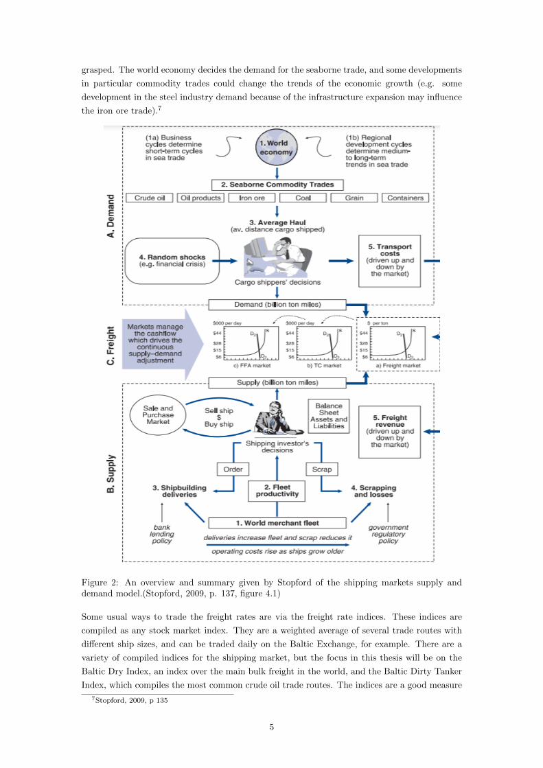
grasped. The world economy decides the demand for the seaborne trade, and some developments
in particular commodity trades could change the trends of the economic growth (e.g. some
development in the steel industry demand because of the infrastructure expansion may influence
the iron ore trade).7
Figure 2: An overview and summary given by Stopford of the shipping markets supply anddemand model.(Stopford, 2009, p. 137, figure 4.1)
Some usual ways to trade the freight rates are via the freight rate indices. These indices are
compiled as any stock market index. They are a weighted average of several trade routes with
different ship sizes, and can be traded daily on the Baltic Exchange, for example. There are a
variety of compiled indices for the shipping market, but the focus in this thesis will be on the
Baltic Dry Index, an index over the main bulk freight in the world, and the Baltic Dirty Tanker
Index, which compiles the most common crude oil trade routes. The indices are a good measure
7Stopford, 2009, p 135
5

for the equilibrium of the shipping markets demand and supply. For more specific definitions,
the reader is referred to the Baltic Exchange’s website.8
As the reader can see in figure 2, the model that is illustrated is the supply and demand model,
with some more intricate definitions and specifications. Since this is a thesis in applied mathemat-
ics and not economics, the details of this model will not be discussed. Two specific phenomenons
are worth mentioning in this context, seasonality and the systems sensitivity to shocks. Season-
ality plays an important role in the seaborne commodities trade, since it can create short term
volatility. Specifically the grain trade can give up to 50% seasonal impact on the bulk freight
rates, since the crops are often harvested in September on the northern hemisphere. In the same
way, Oil and energy is traded seasonally with regard to temperature and weather season, seeing
that more oil is shipped on the northern hemisphere during the Autumn and early winter months
than the during the spring and summer. Shocks on the other hand are unpredictable events that
impact the market with great force. Shocks in the shipping market can come from all sorts of
directions, weather, politics, financial crisis, war and so on. Because of the unpredictability and
the size of the shocks, demand in shipping can change fast, and if it is timed correctly, vast
fortunes can be made(or lost), like the Onassis during the Suez-crisis. During the invasion of
Kuwait, the tanker market went into a boom as demand for tankers to use as storage(floating
storage) for crude oil rallied. Ergo, not all crises are bad for the shipping companies earnings.9
1.1.3 The Covid-19 Pandemic and Freight Market
2019 was a weak year for shipping, trade wars and weaker sentiment led to a decline in demand.
The covid-19 pandemic that overwhelmed the world in the beginning of 2020 led to an economic
crisis which greatly affected the shipping market. UNCTAD estimates that the demand for
shipping will shrink with 4.1% 2020, meaning billions of US dollars. The world was hit by a
simultaneous demand and supply shock which had not been seen before.10
The lockdowns that followed the pandemic caused the demand for crude oil to dive, and prices
for the same commodity followed. Following Saudi Arabia’s failure to agree with OPEC:s pro-
duction cuts, and their ”opening of the taps and valves” was the final blow for the crude oil,
which totally collapsed, and a situation of super contango arose. This led to a surge in tanker
demand, as traders rushed to hire tankers in order to store their oil in order to sell the oil for a
higher price in the future, called floating storage. All tanker segments saw huge peaks in freight
rates and TCE:s during March and April in 2020. As fast as the market rallied, the decline
came all ready in may when the demand for floating storage when the tonnage of floating storage
slumped from 45 million dwt at the end of April to 30 million dwt at the end of May. Demand
for Oil remained significantly lower in mid 2020, and since the OPEC agreement led to lower
output of crude, the tanker market outlook is still looking gruesome, and freights remain low
and very volatile.11
The Bulk market during the covid-19 pandemic was seeing a big slump due to the declining
demand for shipping and overcapacity. Especially during the early outbreak of the pandemic,
since China is the major importer of many bulk goods globally, including iron ore and grains.
8Baltic Exchange, 20209Stopford, 2009, p 143
10UNCTAD, 202011UNCTAD, 2020
6

The bulk market had already seen a tough year 2019, specifically because of lower Brazilian
iron ore export due to the Vale dam collapse. This chain of negative events caused high market
volatility, and the Capesize index of the Baltic Exchange(which is one of the components of the
Baltic Dry Index) went negative(−243) during February and March. Already in June, the same
index had risen to 2267 because of the easing of lockdowns in China and the rallying imports of
iron ore to the same country. The UNCTAD outlook for this market is not very positive either,
overcapacity is still a big problem, and China is mentioned as one of the key features for market
recovery since they are the biggest importers of bulk goods, such as iron ore and grains. 12
1.2 Aim
On account of the events that occurred during the spring of 2020, and the covid-19 pandemic, i.e.
counterintuitive movements in the freights rates in regard to the underlying commodities, the
idea behind this thesis is to analyse these markets. The aim of this project will be to assess time
series over different data, which are believed to hold important information about the maritime
economy and shipping business, in order to create a Vector Autoregression model. This VAR-
model will be used to forecast and develop an analysing tool to predict freight rates and simulate
shocks. In today’s shipping business there are many different freight rates for various types of
cargo, from Very Large Crude Carriers rates to Dry Bulk rates. These rates depend on many
different variables and are entwined with data such as crude oil price, economic growth, world
trade and the second hand market. This thesis will aim to assess these connections.
1.3 Relevance
The shipping business is a trillion dollar business, and it provides work for millions of people.
In today’s global world, the seaborne transport is highly necessary for the global economy.
The relevance in this project comes from the necessity for shipping companies to forecast their
incomes, and the importance of the oil price for the whole world trade according to UN, since it
is both the biggest goods type and affects as bunker fuel for propulsion. The same holds for the
iron ore and the development of the economies and infrastructure, and it is the most important
seaborne bulk goods.
1.4 Problem Formulation
This thesis seeks to analyse and model the following questions
• Will a VAR-process forecast freight rates for oil tankers and bulk better than the simple
univariate ARIMA, when taking into account data such as the Crude oil prices, Iron ore
price, and some other econometric/financial data?
• How will the impulse response function simulate shocks on the freight rates? Which un-
derlying data will have the biggest influence on the freight rates given an impulse?
1.5 Limitations
The limitations of the this thesis are that the focus will be on the bulk and tanker market. Specif-
ically the Baltic Dirty Tanker Index and the Baltic Dry Index will be analysed in the period of
2009-05 to 2020-11, and will be the variables of interest in their respectively model. Although
12UNCTAD, 2020
7

the container shipping market is growing each year, the market is not as easily modelled, and
is therefore not taken into consideration. In general the models that are created consists of a
number of time series, which are analysed together in order to create a good forecast. Although
the models are constructed with macro economic theory as a base, the models will be totally
unbiased in relation to assumed relationships between variables. This means that all the results
from this thesis are based strictly on mathematics and statistics rather than macro-economical
assumptions. The data which is used comes from open source sources, and can be easily retrieved.
The starting point was to also include some sort of data which tracked environmental actions
or sustainability within the shipping business, but since such data has either very low time fre-
quency, or has not been observed for especially long time, this goal is dropped. In the future
when society is more enlightened in these areas, some sort of analysis can perhaps be made, to
investigate if sustainability affects the freight rate pricing. Some other trials are made to include
an exogenous dummy variable in an attempt to model legislation for sulphuric emissions from
the shipping industry in certain areas, but this is also dropped because of lack of time and bad
effects on model diagnostics.
All the mathematical framework used in this thesis achieved their goal. Although it should
be noted that the VAR-modelling is the most basic form of analysing multiple time series. Other
such models which can be of interest are for example VECM, Vector Error Cointegration Model,
or BVAR, Bayesian Vector Autoregression. These are also both often used in econometric mod-
elling. The VAR-model is often used to analyse big macro economic systems, like the relationship
between mortgage rates, housing prices and GDP.
1.6 Previous Work
Two previous work are the main sources for investigation and inspiration for ideas for this thesis.
The first is ”A Novel Approach to Forecasting the Bulk Freight Market” by Vangelis Tsioumas
et al.. In this article the authors try to model the bulk shipping market with BDI as the variable
of interest, some data regarding Chinese steel output, some sort of compiled index of their own
device and the bulk fleets development. The analysis of the VAR-model is performed in first
differences rather than levels. This model is then compared to an ARIMA-model of the BDI, and
the conclusion is that the VAR-model is solid and creates a better forecast than the univariate
ARIMA. The analysis is performed on monthly data between 1999 and 2014. 13
The other article, ”Quantifying the relationship between seaborne trade and shipping freight
rates: A Bayesian vector autoregressive approach” from 2020, is written by Michail and Melas,
and it tries to quantify the relationships between the Baltic Dry Index, the Baltic Dirty Tanker
Index, and the Baltic Clean Tanker Index and their respective underlying commodities. The
method used is a BVAR, Bayesian Vector Autoregression, and the data is on monthly basis.
They found that the commodity trade has a strong impact on the BDI and BDTI, but the Clean
Tanker Index is not so much impacted, and the conclusion is that they can operate on a more
diverse market. They also found a negative correlation between brent oil and the two tanker
indices, and explained that with the use of tankers as floating storage. 14
13Tsioumas et al. 201714Michail and Melas, 2020
8

1.7 Expectations
During the start of this thesis project, a interview was conducted in an informal capacity with
a person working in the shipping business on a chartering company in Sweden. The 30 years of
work experience from the person working at the chartering company said that the models should
be hold simple, i.e. he meant that if the models hold to many time series of arbitrary data, they
would not perform well in forecasting. The limitation of the set of underlying time series should
be to for example oil price, fleet growth and perhaps production/import data according to his
suggestions.
9

2 Theoretical Framework
This section aims to describe the most important mathematical theories that are needed to
understand and implement the models which are used. The main overall theoretical framework
in this section is based on the work of H. Lutkepohl in New Introduction to Multiple Time Series
Analysis. Some various other sources are used when complementary theory is needed.
2.1 Multiple Time Series Analysis and Forecasting
In order to respond and to decide which policy to employ, decision makers at many structural
levels make use of predictions and forecasts of economic of financial variables. If observations of
a time series of interest are available, and that data from the past contains information about
the future, it is possible to use the data in order to forecast the future events. One of the most
common approach and data is to forecast the unemployment rate for a country or a region using
economic data at hand. This approach to forecast may formally be expressed with the following
formula
yT+h = f(yT , yT−1....), (1)
where f(·) is some suitable function or transform of the past observations yT , yT−1.... .
When handling economic variables, the univariate model is seldom enough, since it probably in
addition depends of past values of sometimes multiple other time series. If many time series are
related together, it is reasonable to use this additional information in order to forecast. A formal
expression for this can be
y1,T+h = f1(y1,T , y2,T , ...., yK,T , y1,T−1, y2,T−1....yK,T−1.....), (2)
by denoting the variables y1t, y2t.....yKt and the forecast y1,T+h. A set of time series ykt, k =
1, ...,K, t = 1, ..., T is often called Multiple time series, and y1,T+h the forecast of variable 1.
It is often interesting to investigate the dynamics and impact that different time series can have
between each others. One mathematical model which can be used to model a system of multiple
time series, and their mutual influence on each other, is VAR, Vector Autoregression.15
2.2 Vector Autoregression
The VAR modelling aims to assess the time series which depend on past behaviour of multiple
variables. In the univariate case above, we have that f(·) is a linear function which models the
forecast of the near future (i.e. h=1), the model becomes
yT+h = ν + α1yT + α2yT−1 + ....+ αpyT−p+1 + uT+1 (3)
where it is assumed that the model is using a finite value of past observations p. Further the value
of yT+h will not be the same as the real yT+h. That is why there is an error term, also known
as the forecast error, uT+1 = yT+h − yT+h. In general the assumption is that the observations
in the model are realizations of random variables, and that the same distribution for the data
generating process holds for each period T . With these assumptions, the univariate form of the
VAR is obtained, which is the autoregressive process, AR,
15Luthkepohl, 2005, p. 1
10

yt = ν + α1yt−1 + α2yt−2 + ....+ αpyt−p + ut (4)
where yi and u are random variables for all t. It is also assumed that ut, the forecast errors, are
uncorrelated for different periods T . From this, the general extension into multiple time series is
yt = ν +A1yt−1 +A2yt−2 + ....+Apyt−p + ut (5)
where yi’s are regarded as random vectors on the form yt := (y1,t, ..., yK,t)′ and ν = (ν1, ....νK)
and
A :=
a11,i . . . a1K,i
.... . .
...
aK1,i . . . aKK,i
. (6)
In the model, it is assumed that ut := (u1,t, ..., uK,t)′ is a vector of independent and identically
distributed variables with zero mean.16
2.3 Stable VAR(p) Process
From above it has been established that the general VAR(p), i.e. the VAR process with order
p,is given by the following
yt = ν +A1yt−1 +A2yt−2 + ....+Apyt−p + ut, t = 0,±1,±2, ...., (7)
in which yt is a (K×1) random vector, the Ai:s are deterministic (K×K) coefficient matrices and
ν is a fixed (K×1) vector of model intercept allowing for non-zero mean E(yt) of the model. ut is
a K-dimensional white noise process with the following properties: E(ut) = 0, E(utu′t) = Σu and
E(utu′s) = 0 ∀s 6= t. The covariance matrix Σu is assumed to be non-singular if not otherwise
stated.
In order to get an intuitive sense about this model, the VAR(1) is considered
yt = ν +A1yt−1 + ut. (8)
If the data generation of this process starts at a given time, t = 1, the following system arises
y1 = ν +A1y0 + u1
y2 = ν +A1y1 + u2 = ν +A1(ν +A1y0 + u1) + u2 =
= (IK +A1)ν +A21y0 +A1u1 + u2
...
yt = (IK +A1 + ...+At−11 )ν +At1y0 +
t−1∑i=0
Ai1ut−1
...
(9)
16Luthkepohl, 2005, p. 4
11

From this, it is clear that the vectors y1, ..., yt are all uniquely determined by y0, u1, ...., ut and
also the joint distribution of y1, ..., yt is determined by the joint distribution of y0, u1, ...., ut.
If all the eigenvalues of A1 have a modulus of < 1, the sequence Ai1 will be absolutely summable,
i.e. the infinite sum∑∞i=0A
i1ut−1 exists in mean square. The proof for this can be found in
the reference material of this section but is here omitted. From this fact, the VAR(1)-process
becomes the well-defined stochastic process
yt = µ+
∞∑i=0
Ai1ut−1. (10)
are
µ = (IK −A1)−1ν. (11)
The distributions and joint distributions of the yt are uniquely determined by the distributions
of the ut process. The first and second moments are known to be
E(yt) = µ ∀t ∈ R (12)
and
Γy(h) = E[(yt − µ)(yt−h − µ)′] =∞∑i=0
Ah+i1′ΣuA
i1′. (13)
since E(utu′s) = 0 ∀s 6= t and E(utu
′t) = Σu ∀t ∈ R.
A VAR-process is deemed stable if all eigenvalues of A1 have modulus of < 1 or expressed
mathematically as the following condition
det(Ik −A1z) 6= 0 ∀|z| ≤ 1. (14)
These concepts above can easily be extended to the general VAR(p) process, since for any p > 1 a
VAR(p)-process can be written on the VAR(1)-form. If yt is a VAR(p)-process as defined above,
a corresponding Kp-dimensional VAR(1)-process can be defined as
Yt = ν + AYt−1 + Ut (15)
where
Yt :=
yt
yt−1
...
yt−p+1
, ν =
ν
0...
0
,
A =
A1 A2 · · · Ap−1 Ap
IK 0 · · · 0 0
0 IK 0 0...
. . ....
...
0 0 · · · IK 0
, Ut :=
ut
0...
0
.(16)
12

Following the same structure from earlier in this section, Yt is stable if
det(IKp−Az) 6= 0 ∀|z| ≤ 1. (17)
The first and second moments for the model are given by
µ := (IKp −A)−1ν (18)
and
ΓY (h) =
∞∑i=0
Ah+i′ΣUAi′. (19)
where ΣU := E(UtU′t). Using the K × Kp matrix
J :=[IK : 0 · · · : 0
], (20)
the process yt is obtaind as yt = JYt. Since Yt is a well-defined stochastic process, the same
holds for yt. The mean is E(yt) = Jν, which is constant for all t, and the autocovariance matrix
is given by Γy(h) = JΓY (h)J ′, which is also independent of t. yt is defined as stable if
det(IKp−Az) = det(IK −A1z −A2z
2 − .....−Apzp) 6= 0 ∀|z| ≤ 1, (21)
which is also known as the stability condition. To summarize, a VAR(p)-process is stable if (21)
holds, and
yt = JYt = Jµ + J
∞∑i=0
AiUt−1. (22)
By the definitions stated above, it can be easily seen that the process yt is determined by its
white noise.17
2.4 Stationary Model
A stochastic process is called stationary when its first and second moments are assessed as time
invariant. I.e. a stochastic process, yt is stationary if
E(yt) = µ ∀t ∈ R (23)
and
E[(yt − µ)(yt−h − µ)′] = Γ(h) = Γ(−h)′, ∀t ∈ R, h = 0, 1, 2, ... (24)
The first condition means that yt has a mean vector that is constant for all t. In the same
way, the autocovariance matrix is also independent of t and only depends on the time difference
step, h. If not stated, all quantities are assumed to be finite. It follows from above that a
stable VAR(p)-process also is stationary, i.e. stability implies stationarity, but not necessarily
the other way around. Stable VAR-processes has under usual assumptions time invariant means
and variances and covariances.18
If one of the underlying time series in the VAR(p)-process is deemed non-stationary (i.e. with
I(1) or a trend) by some of the tests that exists, the solution is often to make the process trend-
stationary. This is done by taking the first order differences. First order difference means to
17Luthkepohl, 2005, p. 2418Luthkepohl, 2005, p. 13
13

create a new time series by the following formula y′t = yt−yt−1. The problem is that it is advised
to chose to either estimate a VAR(p)-process in levels (without any differencing at all), or to
estimate it in first differences (all underlying time series are differentiated one time), it is seldom
advised to to have both leveled and differentiated time series in the same VAR-process, only if
there is no co-integration. Here Luthkepohl advises to not differentiate the non-stationary time
series in the VAR-process, since their is a risk that one throws away essential information. If the
VAR-process in levels is stable, then by assumption it is also stationary and further analysis can
be done.19
2.5 Autoregressive Integrated Moving Average-Model
In time series analysis there arises a need to model not only stationary time series, but non-
stationary time series as well. A general model which can handle a big variations of non-stationary
processes is the ARIMA-process, i.e processes that are reduced to ARMA-processes when differ-
entiated finitely many times.
By definition, if d is a non-negative integer, then Xt is an ARIMA(p,d,q) process if :
Yt := (1−B)dXt (25)
is a causal ARMA(p,q) process. This gives that the process Xt satisfies the difference equation
φ∗(B)Xt ≡ φ(B)(1−B)dXt = θ(B)Zt, Zt ∼WN(0, σ2) (26)
where φ(z) and θ(z) are polynomials of degree p and q, and that φ(z) 6= 0 for | z |≤ 1. 20
2.6 Autocovariance and Autocorrelation
As shown above, one of the requirements for a time series to be deemed stationary is that the
value of the time series at different times only depend on the time difference between two points.
In higher order VAR(p) this is illustrated by
yt − µ = A1(yt−1 − µ) + ...+Ap(yt−p − µ) + ut (27)
and the autocovariance function is denoted by Γy(h). For h = 0,
Γy(0) = A1Γy(1)′ + ...+Ap(Γy(p) + Σu (28)
and with h > 0
Γy(h) = A1Γy(h− 1)′ + ...+Ap(Γy(h− p) + Σu. (29)
These equation are know as the Yule-Walker equations, an can be used to calculate Γ(h).21
Because of the unit dependence in the Autocovariance function, it is often more convenient
to use the Autocorrelation function instead when modelling, since it is scale invariant of the
linear dependencies in a model. The Autocorrelation function is given by
Ry(h) = D−1Γy(h)D−1 (30)
19Luthkepohl, 2011, p. 520Brockwell et al, 2002, p. 18021Luthkepohl, 2005, p. 26
14

where D is the matrix with the standard deviations of the components of yt on the main diagonal,
i.e. the main diagonal elements are the square roots of the diagonal elements of Γy(0).22
2.7 Estimations of a VAR(p)-process
In order to estimate the parameters within a VAR(p)-process, the least squares estimate β, which
minimizes the error, needs to be calculated.
Defnintions:Y := (y1.....yT ) (K × T ),
B := (ν,A1, ....., Ap) (K × (Kp+ 1)),
Zt :=
1
yt...
yt−p+1
(Kp+ 1),
Z := (Z0, ...., ZT−1) ((Kp+ 1)× T ),
U := (u1, ....., uT ) (K × T ),
y := vec(Y ) (KT × 1),
β := vec(B) ((K2p+K)× 1),
b := vec(B′) ((K2p+K)× 1),
u := vec(U) (KT × 1),
(31)
where vec is the vector stacking operator. When using the notation above, and t = 1, 2, ...., T ,
the VAR-model can be written in this compact way
Y = BZ + U. (32)
From this the normal equation of the least squares follows as
(ZZ ′ ⊗ Σ−1u )β = (Z ⊗ Σ−1
u )y. (33)
Solving the above stated equation gives the least squares estimator in the following way
β = ((ZZ ′)−1Z ⊗ IK)y (34)
where ⊗ is the Kronecker operator. 23
2.8 Order Selection of VAR(p)
When modelling a set of multiple time series, the problem of selecting the optimal lags, p, arises.
In theory there is not just one right answer to this problem, because if yt is a VAR(p)-process,
it is also formally a VAR(p+1)-process. This holds for the previous assumption that coefficient
matrices which are zero, are not excluded from the model. Henceforth, it is now defined that a
VAR(p)-process, is a process for which all Ap 6= 0 and Ai = 0, i > p. I.e. p is the smallest order
possible for the model.24
When forecasting is the main goal of the VAR(p)-process, it is reasonable to choose order in
22Luthkepohl, 2005, p. 3023Luthkepohl, 2005, p. 6924Luthkepohl, 2005, p. 136
15

a way that reduces the Mean Square Error (MSE). Akaike(1969,1971) suggested to base the
VAR-order selection on a one-step ahead forecast MSE, given by
Σy(1) =T +Km+ 1
TΣu (35)
where m is the lag order for the selected VAR-process, T is the sample size, and K is the
number of time series in the VAR-process. From this it is easy to see that a VAR(p)-process
should be chosen over a VAR(p+i)-process, since the forecast MSE is an increasing function
of the order of the fitted model. In practice, the lag order is selected from different criterion.
The most common among these criterion are the Akaike’s information criterion(AIC), Final
prediction error(FPE), Bayesian/Schwarz information criterion (BIC/SC) and the Hannan-Quinn
information criterion(HQ). Of these, AIC and the FPE are more suited to use when having
samples of up to 60 observations and/or when the main focus for the estimated model is to
forecast, while SC and HQ are more suited when having samples of more than 120 observations
and/or estimating the with the notion of consistency of the model. Infact, Shibata(1980) showed
that also for univariate models the FPE and AIC minimizes the one-step-ahead forecast MSE
asymptotically. 25
2.9 Normality of Residuals
When estimating a VAR(p)-process, the need of normality arises in the underlying data gen-
eration. When estimating the normality of a model, one often investigate the normality of
the model residuals. This is important when performing the impulse response analysis on the
VAR(p)-model.
A stationary VAR(p)-process is Gaussian distributed if and only if the residuals white noise
processes ut are Gaussian. There are different tests to investigate the normality of the residu-
als, one is to investigate the third and fourth moments (i.e. Skewness and Kurtosis) as in the
Jarque-Bera-test.
If the assumption of Gaussian distributed White-Noise residuals cannot be made, different boot-
strap method can be used in order to create new sets of residuals from the data, by drawing
repeatedly from the estimated residuals.26
2.10 Expectation-Maximization Algorithm
When only a subset of the data of interest is available, the Expectation-Maximization(EM) algo-
rithm can be used as an iterative procedure to compute the maximum likelihood estimator. The
EM-algorithm is one of the methods used for imputation of data sets with missing observations.
Let (X1, X2, .......Xn be the sample data set, where observations are missing, with the conditional
density fX|Θ(x|θ) given Θ = θ. From this the log-likelihood function is written below
l(θ;X) = logfX|Θ(X|θ). (36)
Since data is missing, it is assumed that the data X consists of the subsets Y = (Y1, Y2, ...Yk)
which are the observed observations, and Z = (Z1, ...., Zn−k) which are the missing (or latent)
observations of the data set. With X = (Y,Z) the log likelihood for the observed Y is given by
the following
25Luthkepohl, 2005, p. 15126Luthkepohl, 2005, p. 17
16
lobs(θ;Y ) = log
∫fX|Θ(Y, z|θ)νz(dz). (37)
A problem can arise when calculating the integral in order to maximize the log-likelihood, since
it might not be possible to find a closed form of the lobs(θ;Y ). In order to maximize the lobs(θ;Y )
with respect to θ an iterative process with two steps is done, the E-step and the M-step, where
θ(i) is the estimate of Θ and after the ith step. Then the two steps in the (i+ 1)th iteration are
E-step: Compute Q(θ|θ(i)) = Eθ(i))[l(θ;X)|Y ].
M-step: Maximize Q(θ|θ(i)) with respect to θ and put θ(i+1) = argmax Q(θ|θ(i)).
This procedure is repeated until the model convergence on the integral is achieved.27
2.11 Impulse Response Analysis
When applying a VAR(p)-process on a data set of multiple time series, it is often of interest to
see how one variable reacts to an impulse in another variable of interest within a model with a
number of variables, e.g macro-economical or financial variables.
Consider the problem when isolating the shock impact of one variable on another variable, at
a time t = 0. It is supposed that all the variables hold their mean value prior to time t = 0,
yt = µ. Now at time t = 0 one variable s is increased by one unit, to u1,0 = 1. It is now possible
to trace what happens with the system in the periods t = 1, 2...., n if it is assumed that no other
shocks occur, i.e. u2,0 = 0, u3,0 = 0 and so on. In such an event, the mean of the system is of no
interest, but the variations of the variables around their means are, the means of the variables
are set to zero, and ν = 0.
The first column of Ai1 are the yi = (yk,i)′. The elements of Ai1 represent the effect of a
unit impulse in the variables of the model after i periods from t = 0. Because the variables
in a model often have differing scales it may be extended to shocks of different magnitudes by
rescaling the impulse responses. For instances, instead of analysing an unexpected unit shock in
some variable, a shock of a standard deviation in magnitude is used instead. This gives a clearer
visualization of the impulses dynamic and relationship between the variables in the model. In
the impulse response graph, their is often a calculated confidence-interval which is calculated
from the normality of the VAR-model. If the VAR-model is non-normal, the confidence intervals
are bootstrap several times.28
2.12 Forecasting
From earlier theory we know that the optimal h-step forecast is given by
yt(h) = ν +A1yt(h− 1) + ....+Apyt(h− p) (38)
where yt(j) = yt+j , i.e. the timestep as a function of j. If in this equation, the true coefficients
B = (ν,A1, ...., Ap are replaced with their estimates B = (ν, A1, ...., Ap, we get the estimated
forecast
yt(h) = ν + A1yt(h− 1) + ....+ Apyt(h− p) (39)
27Hult, 2019, p. 9028Luthkepohl, 2005, p. 53
17

where yt(j) = yt+j , and thus, the forecast error can be calculated as
yt+h − yt(h) = [yt+h − yt(h)] + [yt(h)− yt(h)] =
h−1∑i=1
Φiut+h−i + [yt(h)− yt(h)](40)
where Φi are the coefficient matrices of the canonical MA-innovations representation of yt, which
for shortness sake is omitted. Under general conditions of the VAR(p)-process forecast, it can
be assumed that the mean of the forecast is zero, i.e. E[yt+h − yt(h)] = 0. From this it is
understood that the forecast is unbiased even with the coefficient estimates. All the us and yt
are uncorrelated if the estimations are done up to a period t, and from this we can calculate the
MSE matrix, Mean Square Error, for yt(h) as the following
Σy(h) := MSE[yt(h)] = E[[yt+h − yt(h)][yt+h − yt(h)]′]
= Σy(h) +MSE[yt(h)− yt(h)](41)
in which
Σy(h) =
h−1∑i=0
ΦiΣuΦi′. (42)
From these equations a result which minimizes the forecast MSE is calculated, in order to retrieve
the best predictor in conformity with earlier results and requirements on the VAR(p)-process.29
2.13 Forecast Error Variance Decomposition
If the innovations which drive the VAR-process could be assessed, another tool for examining
the model is available. The MA(Moving Average)-representation of the process can be written
as
yt = µ+
∞∑i=0
ΦiPP−1ut−1 = µ+
h−1∑i=1
Θiwi (43)
where Θi = ΦiP and wi = P−1ut−1. In this the Σu = PP ′, where P is a lower triangular
non singular matrix with positive diagonal elements. In equation (43) the components of wt =
(w1t, ..., wKt) are uncorrelated white noise with have unit variance, and the covariance matrix
Σw = P−1ΣuP−1′ = IK , where IK is the identity matrix with (K ×K)-elements.
Giving the denotation θmn,i for the mn-th element of the Θi-matrix the h-step forecast error of
the j-th component of yt is
yj,t+h − yj,t(h) =
K∑k=1
(θjk,0wk,t+h + ...+ θjk,h−1wk,t+1). (44)
From equation 44 we get that the forecast error of the j-th component could consist of all
innovations wt = (w1t, ..., wKt). Although obviously some of the components mn,i could be = 0,
so that some of the components disappears. Since the components of wt are uncorrelated, the
MSE of yj,t(h) becomes
E[yj,t+h − yj,t(h)]2 =
K∑k=1
(θ2jk,0 + ...+ θ2
jk,h−1). (45)
29Luthkepohl, 2005, p. 94
18

From this
θ2jk,0 + ...+ θ2
jk,h−1 =
h−1∑i=0
(e′jΘiek)2 (46)
which is often interpreted as contribution of innovations in variable k to the MSE of the h-step
forecast of variable j. Here ei is the i-th column of IK . Dividing equation 46 by the MSE[yj,t(h)]
gives
ωjk,h =
∑h−1i=0 (e′jΘiek)2
MSE[yj,t(h)]. (47)
The last equation gives the proportion of the h-step forecast error variance of variable j through
the innovations wkt. If wkt can be related to variable k, wjk,h is the representation of the
properties of the h-step forecast error variance, which is accounted for by innovations in variable
k. Thus, the forecast error variance is decomposed into parts which are accounted for by the
innovations in the different variables of the model. The h-step forecast MSE-matrix is given by
Σy(h) = MSE[yt(h)] =
h−1∑i=0
ΘiΘi′ =
h−1∑i=0
ΦiΣuΦi′. (48)
in which the diagonal elements are the MSE:s of the yjt variables which is shown before.30
30Luthkepohl, 2005, p. 63
19

3 Data
For this thesis, two sets of time series are made, one for the Tanker-Oil-model, and one set for the
Bulk-Iron-model. The goal in the data search is to find as equal and similar explanatory market
data for each model as possible. But, as the reader may note, there is not always a perfect data
counterpart available between the different parts of the industry or markets.
All data series are measured between 05-2009 and 06-2020, striving to have weekly measurements.
The forecasts are then made between 06-2020 and 11-2020, 26 weeks forward. The reason why
weekly data is chosen over monthly or quarterly is that the big movements(i.e. volatility) in oil
and freight markets that occurred during the financial crisis and the covid-19-pandemic would
not have been so well captured with lower time resolution. In the cases where only monthly
measurements are available, statistical imputations are performed in order to increase the fre-
quency of the data series. As many relevant data series as possible are sought in order to create
a VAR(p)-model that is representative for the underlying market. The final number of observa-
tions used to create the models is n = 595, which is divided into n = 569 for model creation,
and n = 26 for validation/forecast comparison of the indices. The data is retrieved from several
different sources, the main part from Baltic Exchange and Clarkson’s, and some open source
financial data.
3.1 Time Series in Oil-Tanker-Rates-Model
The following nine time series are used in the VAR(p)-process that is created in order to forecast
and analyse the Tanker-Oil-market.
Baltic-Dirty-Tanker-Index(BDTI)
The main variable of the Oil-Tanker-model. Compiled index of the most common trade routes
for dirty tankers. Published every day by the Baltic Exchange as a market benchmark.31
Brent Oil Price
Spot price of Brent Oil in US-dollars per barrel, the most commonly traded oil contract. Priced
continuously during market hours, data extracted on weekly basis from EIA (Energy Information
Administration).32
Tanker Earnings
Average of shipping companies tanker earnings compiled over different sizes of tankers. Measured
in dollars per day, weekly data is extracted from the Clarkson register. 33
Dollar Index
Index or measure of the US dollars strength compared to a basket of foreign currencies. A high
index indicates a strength in US dollars, and a low index indicates weakness. Priced continuously
during market hours, data extracted on weekly basis from Investing.com34
31Baltic Exchange, 202032EIA, 202033Clarksons, 202034Investing.com, 2020
20

Libor
London Interbank Offered Rate, is the 3-month daily updated investment rate. Libor is the most
standard investment rate and is used as a global benchmark for short term investment rates. The
time series consist of the logarithmic returns of the LIBOR-rate. 35
Second Hand Tanker Price
Weekly assessments of the price of a five year old vessel measured in US-dollar per tonne. In this
case the Tanker types that are considered are VLCC- and Aframax-size, extracted from Baltic
exchange.36
Singapore Tanker Arrivals
Time series over the monthly tonnage of oil-tanker arrivals, only vessels that are more than 75
gross tons are included. Measured in thousands tons. compiled by the ”Maritime and Port
Authority of Singapore”.37
US Oil Imports
Assessment of the total weekly imports of crude oil to the United States. Measured in thousand
barrels and compiled by the EIA (Energy Information Administration).38
Fleet Growth
Relative change of the growth of the total world fleet from month to month. Data collected from
the Clarkson’s register.39
Time Series Min Max Mean Standard DeviationBDTI 431.0 3194.0 1020.3 440.863
Brent Oil Price 14.24 141.07 76.05 27.10494Tanker Earnings 5752 98094 18137 11659.07
Dollarindex 72.10 103.01 87.89 8.499Libor -0.458 0.478 -0.002 0.050
Second Hand Tanker Price 51.93 162.90 73.12 18.77Singapore Tanker 35418 74675 50574 8051
US imports 4900 11153 7919 970Fleet Growth -0.013 0.012 -0.003 0.003
Table 1: Table of summary statistics for the time series in the Tanker-Oil-model.
3.2 Time Series Bulk-Iron-Rates-Model
The following time series are used in the VAR(p)-process that is created in order to forecast and
analyse the Bulk-Iron-market.
35macrotrends.net, 202036Baltic Exchange, 202037MPA Singapore, 202038EIA, 202039Clarksons, 2020
21

Baltic-Dry-Index(BDI)
The main variable of the Bulk-Iron-model. The Baltic-Dry-Index is a composite index of the
weighted dry bulk timecharter averages of the Capesize (40%), Panamax (30%) and Supramax
(30%) indices. Published every day by the Baltic Exchange as a market benchmark.40
Iron Ore Price
Iron ore prices used in this thesis are Iron Ore Fine China Import 62 percent grade Spot Cost.
This contract is delivered in Tianjin China and the ore is used to make steel for infrastructure
and other construction projects. Priced continuously during market hours, data extracted on
weekly basis from Investing.com 41
Bulk Earnings
Average of bulk earnings compiled over different sizes of bulk. Measured in dollars per day,
weekly data is extracted from the Clarkson’s register. 42
Dollar Index
Index or measure of the dollars strength compared to a basket of foreign currencies. Priced
continuously during market hours, data extracted on weekly basis from Investing.com43
Libor
London Interbank Offered Rate, is the 3-month daily updated investment rate. Libor is the most
standard investment rate and is used as a global benchmark for short term investment rates. 44
Second Hand Bulk Price
Weekly assessments of the price of a five year old vessel measured in US-dollar per tonne. In this
case the Bulk types that are considered are Cape-size and Panama-size, extracted from Baltic
exchange.45
Singapore Dry-Bulk Arrivals
Time series over the monthly tonnage of bulk-freighter arrivals, only vessels that are more than
75 gross tonnes are included. Measured in thousands tonnes. Compiled by the ”Maritime and
Port Authority of Singapore”.46
Australian Metal Bulk Export
Aggregated data from Australia considering the value in Australian Dollars of ”Metalliferous
ores and metal scrap” that is exported every month. Data is collected by the Australian Bureau
of Statistics and published every month on their webpage.47
40Baltic Exchange, 202041Investing.com, 202042Clarkson’s, 202043Investing.com, 202044macrotrends.net, 202045Baltic Exchange, 202046MPA Singapore, 202047ABS, 2020
22

Fleet Growth
Relative change of the growth of the total world fleet from month to month. Data collected from
the Clarkson’s register.48
Time Series Min Max Mean Standard DeviationBDI 290.0 9379.0 1490.9 798.2
Iron Ore Price 38.28 188.25 100.14 37.4Bulk Earnings 3504 57804 10634 4819.6Dollar index 72.10 103.01 87.89 8.499
Libor -0.458 0.478 -0.002 0.050Second Hand Bulk Price 16.11 50.89 30.38 8.38
Singapore Dry Bulk 37888 78651 58640 8799Australian Export 3003 12904 7147 1739
Fleet Growth -0.013 0.012 -0.003 0.003
Table 2: Table of summary statistics for the time series in the Bulk-Iron-model.
3.3 Imputations and EM-algorithm
In order to elevate the time frequency to weekly in the time series which are only possible to find
in monthly frequency, the Expectation-Maximization-algorithm is applied. This specific method
assumes that the data which is imputed is asymptotically normally distributed, and therefore all
the time series which are imputed via this EM-algorithm are first investigated via the QQ-plot.
Results from this can be found in Appendix B. The following time series are imputed using the
EM-algorithm,
• Australian Ore Export
• Fleet Growth
• Singapore Tanker Arrivals
• Singapore Oil-Bulk Throughput
with successful normal EM-convergence for all of them. All time series are imputed 5 times, and
then the average of all 5 imputations are taken in order to make a new time series with weekly
time-frequency. The graphs over the fitted distributions via the EM-algorithm can be seen in
the Appendix B of this thesis.
3.4 Stationarity
Following the mathematical framework when establishing a VAR(p)-model, the necessity for a
stationary VAR(p)-process is given. In order to investigate all the underlying time series in the
VAR(p)-processes, a test for stationarity is performed on them one by one. The test that is used
is the Phillips-Perron test, which does not require a selected lag before testing for unit roots.
For the following time series the null-hypothesis, i.e. that the time series has a unit-root, could
not be rejected on p ≤ 0.05 significance level
• Dollar index
48Clarksons, 2020
23

• Brent Oil
• Iron Ore
• Second Hand Price Tankers
• Second Hand Price Bulk.
As before mentioned, the VAR(p)-processes stationarity is not completely dependent on the sta-
tionarity of each of the underlying time series but on the systems stability. No transforms is
exercised on the data and the plots of the original time series and their residuals can be found
in the Appendix A of this thesis.
24

4 Method
The time series that are part of the two VAR(p)-models that are estimated are chosen because
of the sought connection between them. In the light of this, the VAR(p)-models are completely
unbiased in that regard, and simply takes into account the observations of the input data.
The two ARIMA-models which are also estimated, are purely estimated from the two respective
freight rate indices, and therefore also independent and completely unbiased.
4.1 R
The modelling and mathematical analysis of the data is performed in the statistical compu-
tational software R, specifically R version 4.0.1. Specific important packages that are used to
perform the analysis are the following
• VAR Estimation package: vars49
Package for estimations of VAR-models, diagnostics of models, the impulse response func-
tion and forecasting.
• EM-algorithm package: Amelia50
Package for multiple imputations via the Expectation-Maximization algorithm.
4.2 Lag-Selection
In order to select the lag order for the models the different criterion are applied after binding
together the time series. It is important to weigh between model adequacy and not choosing to
many lags. Akaike’s information criterion(AIC), Finalprediction error(FPE), Bayesian/Schwarz
information criterion (BIC/SC) and the Hannan-Quinn information criterion(HQ) are all anal-
ysed for both models. As written before, for VAR(p)-processes which are estimated in order to
mainly do forecasts, minimizes the forecast MSE when selecting lags given by Akaikie’s Infor-
mation Criterion and Forecast Prediction Error, and thus these criterion will be dimensioning in
this case.
4.3 Model Diagnostics
When the lag order is selected for each model respectively, a number of diagnostic measures
are applied to the model, in order to check if the theoretical assumptions holds. The following
sections will give brief descriptions of them.
4.3.1 Serial Autocorrelation
A test is performed in order to investigate whether the models suffers from serial autocorrelations.
The test computes the multivariate Portmanteau-test to check the models serially correlated
errors. The null hypothesis is that there is no serial autocorrelation in the model, and the
significance level is p = 0.05. Since serial autocorrelation is undesirable one wants to confirm the
null hypothesis.
49Pfaff et al, 201850Honaker et al. 2019
25

4.3.2 Heteroskedasticity
Heteroskedasticity or ARCH(Autoregressive conditional heteroskedasticity)-effects in the models
are undesirable, since it means that different observations have different variances over time. In
order to test whether the models suffer from this, an ARCH-LM(Lagrange Multiplier)-test is
performed. The null hypothesis is that the model does not suffer from heteroskedasticity, on the
significance level p = 0.05.
4.3.3 Test of Normal Residuals
For the impulse response analysis the residuals of the fitted models needs to be normally dis-
tributed, otherwise the need of bootstrapping the confidence intervals for the impulse response
arises. In order to test the normality, the Jarque-Bera test is applied to the residuals of the
estimated VAR-model and the null hypothesis is that the residuals are non-normally distributed
with significance level p = 0.05.
4.3.4 OLS-Estimates
In order to check the stability of the VAR(p)-models, it is checked if the eigenvalues of the
Ordinary-Least-Squares estimates have a modulus of < 1. This is investigated graphically. This
step is important since it decides whether the theoretic assumptions about stability(and station-
arity) are feasible for these models.
4.4 Impulse Responses
The impulse responses is calculated from giving the underlying time series an impulse of one
standard deviation and then plotting the response in the variable of interest, i.e. the freight
rates. The response is the magnitude of the deviation from the mean of the freight rate. The
confidence intervals are bootstrapped and the number of bootstrap runs is set to n = 200, and
the confidence intervals are set to 95%. The number of lags for which the impulse response is
analysed is set to h = 26 in order to correspond to half a year in real time.
4.5 ARIMA-Model Estimation
The univariate time series of the BDTI and the BDI are estimated and fitted with an ARIMA-
model. In order to find the magnitudes of the lags, integrations and any seasonality, (p, d, q)(P,D,Q)m,
a grid search with all possible configurations is performed with the Akaike information criterion
(AIC) as the dimensioning measure in order to retrieve the best estimations.
4.6 Forecasts
Both the estimated VAR-models and the ARIMA-models are used to create forecasts of the
freight rate indices BDTI and BDI. Forecasts are performed with both a mean forecast, and the
95% confidence intervals. The number of lags on which the forecasts are performed is h = 26,
which in weeks represent half a year. The forecasts are done from June 2020 forward to the last
week of November 2020. The forecast means are then compared with the real data for the same
period, and plotted. The RMSE (Root Mean Squared Error) and MAE(Mean Absolute Error)
are calculated in order to assess the goodness of fit on the real data, and to see if the VAR-model
or ARIMA-model for the respective indices produces the best forecast.
26

4.7 Forecast Error Variance Decomposition
In order to investigate the contribution of each time series to the VAR-models, a Forecast error
Variance Decomposition(FEVD) of each VAR-model is made. These two decompositions are
made to see how much each of the underlying time series effects the forecasts of the BDTI and
the BDI. The FEVD:s are made for h = 12 lags forward. The results are presented as how many
percent of the forecast variance each time series contribute with at the different lags.
27

5 Results
5.1 Final Models
Here follows the results for the final models and their diagnostics.
5.1.1 Final VAR(p)-models
After performing the lag-selection analysis, the following results in the table are given for the
two models respectively.
Model AIC HQ BIC FPEOil-Tanker-rates (BDTI) 7 2 2 7
Iron-Bulk-rates (BDI) 5 2 2 5
Table 3: Table of results and suggested lags from performed lag-selection for each model withfour different criterion.
From this it is decided that the Oil-Tanker-rates model is given the lag p = 7, i.e., VAR(7) follow-
ing the Akaike Information Criterion and the Forecast Prediction Error, and the Iron-Bulk-rates
model is given the lag p = 5, i.e. VAR(5) with the same reasoning.
After deciding the respective lag for each model, the diagnostics results are assessed, and the
results from those are presented in the table below.
Model Serial Autocorrelation ARCH-test NormalityOil-Tanker-rates p = 0.4029 p = 1 p < 2.2 · 10−16
Iron-Bulk-rates p = 0.4258 p = 1 p < 2.2 · 10−16
Table 4: Table of results from performed diagnostic tests on the two models.
From the diagnostics tests it is clearly seen that neither model suffers from serial auto-correlation
or any ARCH-effects, and further analysis with given theoretical assumptions could be done with-
out violation. As can also be seen, neither model has normally distributed residuals, and therefore
the confidence intervals of the impulse-response-functions are bootstrapped several times.
The stability test rendered that all OLS-estimates eigenvalues have a modulus of < 1, which can
be seen in the graphs in Appendix C.
5.1.2 Final ARIMA-models
From the performed grid search with Akaike Information Criterion as the dimensioning measure,
the following orders for the ARIMA-models are estimated
Time Series p d q P D Q mTanker Index(BDTI) 1 0 1 0 0 1 52Dry-Bulk Index(BDI) 1 0 3 2 0 0 52
Table 5: Table of results from the AIC order selection for the SARIMA-models of the freightrates.
The models retrieved from the ARIMA-estimations are both SARIMA:s with a seasonal
component of m = 52. The table of coefficients are
28

Time Series φ1 θ1 θ2 θ3 Φ1 Φ2 Θ1 µTanker (BDTI) SARIMA 0.8878 0.1066 - - - - 0.1167 772.8054
Bulk (BDI) SARIMA 0.9605 0.3535 0.1790 0.0153 0.1066 0.0341 - 1362.3372
Table 6: Table of coefficients of the estimated SARIMA-models.
5.2 Impulse responses
5.2.1 Oil-Tanker-Model
Each underlying time series in the models is given an impulse of magnitude one standard de-
viation, and the impact on the freight rate is estimated. The plots can be seen below for the
Oil-Tanker-Model.
Figure 3: Plots of the impulse responses of Baltic-Dirty-Tanker-Index given shocks of one stan-
dard deviation in all the underlying time series of the model. The red dashed lines are the 95%
confidence intervals of the estimated shocks.
29

5.2.2 Iron-Bulk-Model
Figure 4: Plots of the impulse responses of Baltic-Dry-Index given shocks of one standard devia-
tion in all the underlying time series of the model. The red dashed lines are the 95% confidence
intervals of the estimated shocks.
30

5.3 Model Forecasts
The graphical results of the forecasts of the VAR- and ARIMA-processes are shown below.
Figure 5: VAR(7)-forecast of the BDTI, h = 26 lags forward, with confidence intervals at 95%.The real data for the period 2009-05 to 2020-06 in black and the forecast in blue.
Figure 6: The ARIMA-forecast and real data of the BDTI. The forecast is h = 26 lags forward,with confidence intervals of 95%
31

Figure 7: VAR(5)-forecast of the BDI, h = 26 lags forward, with confidence intervals at 95%.The real data for the period 2009-05 to 2020-06 in black and the forecast in blue.
Figure 8: The ARIMA-forecast and real data of the BDI. The forecast is h = 26 lags forward,with confidence intervals of 95%
32

5.3.1 Forecast Comparisons
In this section, the ARIMA-models forecasts and the VAR-models forecasts are compared with
the real data for the period of June-2020 to November-2020, 26 weeks of data. The real data in
the graphs stretches the whole of 2020 to show the impact of the covid-19 on the Freight rates.
The forecast are from the first week of June 2020 and 26 weeks forward.
Figure 9: Actual BDTI-data compared to the two forecast models made with ARIMA and VARrespectively. The real data displayed is fore the whole of 2020.
Figure 10: Actual BDI-data compared to the two forecasts models made with ARIMA and VARrespectively. The real data displayed is fore the whole of 2020.
33

The Root Mean Square Error(RMSE) and Mean Absolute Error(MAE) between the estimated forecasts and
the real data is calculated.
BDTI RMSE MAEVAR-Forecast 119.46 105.40
ARIMA-Forecas 288.74 268.03
BDI RMSE MAEVAR-Forecast 796.52 744.29
ARIMA-Forecast 566.19 467.81
Table 7: Table of RMSE and MAE for the estimated forecasts and real data.
5.4 Forecast Error Variance Decomposition
The results from the Forecast Error Variance Decomposition follows in both graphical and tabular forms for
better understanding.
Figure 11: Forecast Error Variance Decompostion of the BDTI, h = 12 lags forward.
Lags BDTI Earnings Brent US Libor Dollar Second Growth Singaporeh = 1 1.0000 0.0000 0.0000 0.0000 0.0000 0.0000 0.0000 0.0000 0.0000h = 2 0.7258 0.2625 0.0080 0.0007 0.0011 0.0003 0.0002 0.0003 0.0011h = 3 0.6889 0.2702 0.0114 0.0067 0.0115 0.0032 0.0005 0.0069 0.0007h = 4 0.6362 0.2997 0.0117 0.0153 0.0194 0.0031 0.0006 0.0135 0.0006h = 5 0.5847 0.3101 0.0189 0.0242 0.0405 0.0069 0.0013 0.0127 0.0006h = 6 0.5489 0.2956 0.0269 0.0319 0.0712 0.0114 0.0026 0.0109 0.0006h = 7 0.5238 0.2974 0.0306 0.0434 0.0716 0.0135 0.0086 0.0103 0.0008h = 8 0.4915 0.3023 0.0312 0.0604 0.0690 0.0209 0.0137 0.0100 0.0009h = 9 0.4743 0.2889 0.0313 0.0786 0.0732 0.0243 0.0184 0.0099 0.0009h = 10 0.4598 0.2764 0.0312 0.0948 0.0770 0.0256 0.0242 0.0100 0.0010h = 11 0.4495 0.2648 0.0315 0.1088 0.0777 0.0280 0.0281 0.0105 0.0011h = 12 0.4418 0.2558 0.0313 0.1193 0.0780 0.0304 0.0311 0.0108 0.0014
Table 8: The specific results for the Forecast Error Variance Decomposition of the BDTI for all underlying timeseries.
34

The results from the Forecast Error Variance Decomposition follows in both graphical and tabular forms for
better understanding.
Figure 12: Forecast Error Variance Decomposition of the BDI, h = 12 lags forward.
Lags BDI Earnings Second Libor Iron Dollar Singapore Australia Growthh = 1 1.0000 0.0000 0.0000 0.0000 0.0000 0.0000 0.0000 0.0000 0.0000h = 2 0.8404 0.1509 0.0006 0.0038 0.0011 0.0000 0.0001 0.0008 0.0022h = 3 0.7345 0.2483 0.0011 0.0058 0.0033 0.0006 0.0022 0.0010 0.0031h = 4 0.6638 0.3070 0.0027 0.0083 0.0045 0.0013 0.0074 0.0018 0.0032h = 5 0.6156 0.3414 0.0024 0.0093 0.0048 0.0012 0.0181 0.0020 0.0050h = 6 0.5872 0.3535 0.0022 0.0084 0.0049 0.0012 0.0330 0.0028 0.0069h = 7 0.5695 0.3551 0.0020 0.0075 0.0052 0.0010 0.0464 0.0044 0.0089h = 8 0.5571 0.3506 0.0018 0.0073 0.0058 0.0010 0.0591 0.0067 0.0105h = 9 0.5466 0.3434 0.0017 0.0076 0.0069 0.0013 0.0702 0.0095 0.0128h = 10 0.5364 0.3344 0.0016 0.0082 0.0084 0.0021 0.0808 0.0122 0.0158h = 11 0.5268 0.3253 0.0016 0.0087 0.0101 0.0034 0.0898 0.0151 0.0193h = 12 0.5181 0.3166 0.0016 0.0091 0.0117 0.0051 0.0971 0.0179 0.0228
Table 9: The specific results for the Forecast Error Variance Decomposition of the BDI for all underlying timeseries.
35

6 Discussion
6.1 Analysis of Data
There is always a trade off between information and time resolution when handling time series.
It is only recently, with the big data trend, that there has been an increase in data collection,
i.e. increasing the collecting frequency. Given that much happened during short time intervals
both during the financial crisis and the covid-19-pandemic, the choice to perform the analysis
on weekly data is justified with the information gain. Since the results from the EM-algorithm
are satisfactory, and also the overall performance of the models, the data used is deemed good
enough. The choice to impute the data instead of interpolate is reasonable in the regard that
there is a higher chance of some noise in the data than a straight or polynomial line between the
monthly data points.
Another trade off is if the input time series in the models should be in levels or first differ-
ences, depending on if any of them has a high probability of non-stationarity. Either there is a
completely trend-stationary model but interesting data is thrown away, and vice versa. This is
debated intensively, and Lutkepohl is one of those proposing to analyse in levels as long as the
VAR-process is stable, which is the case with these models. VAR:s that are used in economics
to determine econometric long term relationship are also more sensitive since the interest often
lies in specific point estimates rather than general forecasts. The choice to perform this analysis
in levels, with some non-stationary time series is sound since the VAR-models that are created
are proven to be stable.
6.2 Analysis of Final Models
The final VAR(7) and VAR(5)-processes are deemed solid from a mathematical point of view.
The model diagnostics give stable results, and the models can be used for their purposes. Even
though the reader may notice that the proposed lags used for the model are a bit high, it must
be taken into consideration that these models are based on weeks, and not months which is more
common. Basing the lag-selection on the AIC and FPE is also sensible since this thesis main
task is to produce forecasts, albeit that the BIC and HC perhaps would give ”better” model
OLS-estimates. In the end the creation of the models is about getting reliable models for a given
problem, and not best estimates of coefficient matrices.
After producing the first forecasts, sub models could have been investigated in order to see
which data that contributed more, and which subset of time series that gave the best forecasts.
Guidance for this procedure could have been taken from the FEVD, perhaps by throwing out
the time series which had to low values. This is although not a solid method, but could be a
way to reduce the models and perhaps get better forecasts. Since there is not a smooth way to
perform a grid search of the time series contributions to the VAR-processes, this is not performed.
The ARIMA-models that are retrieved from the AIC grid search are deemed stable and solid for
the task of forecasting. The seasonality of one year(52 weeks) in both models is easily under-
stood, since much economic procedure is based on cyclic seasonality of our society. Both of them
lack any order of integration, echoing the tests of stationarity that showed that both their data
generating processes are at least trend stationary according to the Phillips-Perron test.
36

6.3 Analysis of Impulse Responses
Given the results from the Impulse Response Analysis, it can be said that all time series in this
model have an impact, more or less, on the freight rates. Given the extreme market volatility
that occurred during the covid-19 pandemic it is interesting to see the two market differences,
in the sense that shocks in similar underlying time series, or the three that both models have in
common, affect the models differently. Since their are 16 impulse responses, all will be briefly
commented, but all are interesting in their own right. In almost all om them the zero line in the
impulse response is contained via the confidence intervals, and given that, their can not be an
exclusion that the shock can be zero. In summary the answer to the research question is that it
is plausible to estimate market shocks impacts on the freight rates indices.
It is interesting to see that both oil price and iron ore price are not the impulse responses which
yields the shock with highest amplitude. They both peter out at around 20-25 lags. Although it
can clearly be seen even mathematically that the BDTI are higher for the first 10 lags, showing
probably the effects of the higher demand indicated by increase in the price of oil. While iron
ore price on the other hand jumps up and than decays, this could symbolise the higher demand
in iron ore, and therefore a higher demand to transport it. The Vale dam collapse that forced
negotiated trade routes to be changed since the ore is needed to be found elsewhere, and prices of
ore increasing is a typical example. The oil price increase does also create costs for the shipping
companies, since fuel oil is the main propellant for ships today. This should give a positive effect
on BDTI, since all shipping companies will have higher costs. It could be argued that the oil
price should also be included in the bulk model, to investigate the effects fuel costs have on the
Bulk-market.
The difference between the US oil import shock and the Australian ore export is interesting,
since it explains two significant market situations. When the US slowed down its own oil import,
the tanker market(and oil producers) found other routes to transport and sell the oil on, i.e. the
market recuperates faster since it is more adapted. What we can see is that a positive shock
in oil import gives a negative response in the freight rate, probably because of over supply in
the US, and that leads to lower need of imports the following period. This effect maxes out at
week 10, and then slowly retracts to zero. On the other hand, Australia is over 50% of the ore
exporting market of ore, and the shock in its export slowly lower the freight rate and then after
about 10 weeks hold the same level for the rest of the impulse response period. This could also
be explained with short term oversupply, and that iron ore is probably more slowly consumed
than crude oil. We can also look at the ratio between standard deviation and mean for both
US imports and Australian ore export, and it is clearly seen that the Australian ore exports has
bigger standard deviation, which could result in a higher probability of longer term oversupply
given a shock, resulting in lower demand for bulk freight the following time period. Both the US
oil independence and Vale dam collapse probably well estimated with impulse responses, since
US imports can vary depending on domestic production, and the import they still have saturates
the market rather quickly. The Vale dam collapse gave an over supply of bulk ships that where
chartered on the specific routes, decreasing the ore export from Brazil drastically and increasing
it from Australia in turn.
The reaction to shocks in financial data are as expected. A shock in Libor increase the freight
rates on short term, and then peters out, the Bulk index decreasing to under zero while the
37

Tanker stays above. An increase in Libor means higher loan rates, and therefore probably less
investments, which is a mechanism that probably impacts the bulk market more, since that mar-
ket is more driven by big investment cycles rather than consumption. The same hold for dollar,
since many investments world wide are made in dollar, an increase in dollar means higher cost
for domestic investments, while for the oil market, higher dollar index means that for example
OPEC countries get paid more for their oil in domestic currencies since oil is almost always
priced in dollars.
The impulses in Earnings simulate approximately the same movements, which is not surprising.
The reader can clearly see that the earnings times series and the freight rate indices covaries,
which is obviously because the higher the freight rates, the higher the earnings for the shipping
companies.
The fleet growth and second hand price shocks show symptoms of the same real pricing mech-
anisms in the freight rates. If the demand for second hand vessels grow, or the orderbooks for
new ships are filled, that usually indicates that the markets demand for seaborne trade is high,
and their is no supply-demand equilibrium. Freight rates increase in the short term, and then
when the demand either stabilizes or recesses, the freight rates slumps because of an oversupplied
market.
For the impulse responses regarding the data from Singapore, i.e. tanker tonnage arrivals and
dry-bulk arrivals, the suggested impacts for the shocks differs completely. The Tanker arrivals
data seems to have a very low contribution to the model in total, and therefore its impulse re-
sponses is disregarded on that note. The Bulk arrivals to Singapore on the other hand has the
greatest negative impact of all impulse responses. This is perhaps driven by the same market
mechanisms as in the case with the Australian ore export, but that is more a conjecture.
6.4 Analysis of Forecasts
As can clearly be seen from the results of the measures used to estimated the forecast precision,
their are deviating results for the different market models. This is not surprising if one inspects
the Forecast Error Variance Decompositions also, and contemplate the differences between the
markets. The VAR-model used for forecasting the BDTI has overall better performance from the
underlying time series than the VAR for the BDI. In the BDTI almost all variables contribute
with at least ≥ 1% of the forecast variance, except the Singapore oil data. This is not echoed in
the BDI forecast, where several contributions are ≤ 1%. Even the iron ore price has surprisingly
low contributions. In the end, all endogenous variables in these models contribute more or less to
the forecasts. It is also interesting to notice that in the freight rates only around 50% of forecasts
error variance comes from its own innovations.
Neither the ARIMA:s or the VAR:s performs a perfect forecast of the freight rates, but there are
some interesting observations. The actual BDTI does not exhibit any big volatile movements
during the forecast period, while the BDI exhibits rather big movements in short time.
The Tanker-Oil-market seems to have stabilized during the summer and fall. Given that many
countries, especially China and the US, almost hoarded oil, both for commercial and strategic
reserves during the spring 2020, the overall demand has slumped. The ARIMA-model probably,
38

by experience from the cyclically seasonal data from before, expects a increasing demand for
oil tankers during the fall, due to the colder seasons kicking in. This did not happen, since the
stores are more or less at full capacity, and because of lockdowns, the aviation industry is also
grounded, decreasing demand for oil further. The performance of the VAR is very satisfactory,
especially during these extreme market conditions. In the end, the dirty tanker market is only
dependent of oil as commodity, which makes it easier to aggregated a VAR-model, since the
input data is more obvious and easily determined.
The Bulk-market seems to rally during the beginning of the second half of 2020, around the
same time as the lockdowns in several countries eased over the summer. The ARIMA-forecast,
precisely as in the Tanker-forecasts, expects the seasonal increase in freight demand, because of
harvest season and other seasonal economic indicators, pushing it slightly upwards. During the
same period, the VAR-model is decreasing down to new lows. The VAR-models weak perfor-
mance here is obvious. The bulk market is more dependent on several different commodities, and
not just one as in the dirty tanker market. The iron ore only contributes with about a third of
the overall goods that is transported via seaborne bulk, and a more solid model should have per-
haps had more focus on several commodities rather than other economic and financial indicators.
Regarding the information and suggestions from the informal interview, the results differ between
the different markets, i.e. it is probably better with a simple model focusing on commodities for
the bulk market, but not in the tanker market. Although they are anecdotal, it is interesting
that from a mathematical point of view, the suggestions to keep the models simple is probably
right, in bulk especially.
6.5 Further Research
Further research that is suggested is to perhaps do some more advanced multiple time series
analysis. Perhaps perform a Vector Cointegration Model, and to see if there are long run re-
lationships between the time series, and if it would be better performed in first differences or
levels. A BVAR would also be interesting to test, assigning prior probabilities rather than just
estimate from given data. Another interesting development would be to take a more machine
learning approach to create a forecasting model, for example an LSTM or some other Artificial
Neural Network method.
On the data front, some data for sustainability or environmental impact would be highly in-
teresting to use in these models, given that this is a more and more important subject today
than it is 15 years ago. Could a shipping company increase their freight rates if they have a
sustainable edge? Here it could also be included to lift the question of different shipping fuels
and their impact on the forecasting and impulse responses, since emission friendly fuels often
cost more.
There could also be some comparisons between models with different time resolutions. For
example, does a VAR-model perform better on weekly basis or monthly. Given the inconsistent
way we reference time, there could possibly be some error sources in this. There is also room for
a VAR (or more advanced model tools) on daily basis, since many of the used time series in this
model are measured/priced every day (e.g. BDTI/BDI, oil price/iron ore price, libor, dollar).
39

7 Conclusion
In conclusion the results from this thesis are interesting and satisfies both expectations and the
research questions. The models are solid and properly assessed, and they work given the purpose,
even though the market conditions are the most volatile in many years.
All the impulse responses corresponds in plausible ways to real market mechanisms and expec-
tations, and not just depend on their own mathematical innovations. This makes them plausible to
be used efficiently as an instrument of analysis for the shipping industries, since shocks are among
the main features driving the market, especially in the wake of the covid-19 pandemic, which made
markets conditions extreme.
For the BDTI, the VAR-model is superior in forecasting, while in case of the BDI, the ARIMA-
model outperformed the VAR. With different results for the two different markets regarding the
forecasts, it is deduced that the dirty tanker market is simpler to forecast due to its obvious depen-
dence on only one commodity while the dry bulk market is more intricate and depends on several
commodities, and not just iron ore. It is also deduced that the commodities pricing in themselves
are not the most important indicator for forecasts, rather than other more market describing data.
Given that the main drivers of these markets are seasonality and black swan events, it will always
be very hard to give a fair and completely accurate forecast of these indices. The forecasts are never
expected to describe this volatile market perfectly rather than give guidance.
In future, further research is needed, and the dependence on these models for market references
are limited, but they can give an understanding of which data that drive the seaborne freight indus-
try.
40

Appendix A: Original Time Series
Figure 13: Plots of all the time series in the models, with there first difference and ACF:s andPACF.
41

Figure 14: Plots of all the time series in the models, with there first difference and ACF:s andPACF.
42

Appendix B: EM-Algorithm Results
QQ-plots of Imputed Time Series
Figure 15: QQ-plots of the distributions of the data series that are imputed, plotted against anormal distribution.
43

Distributions of Fitted Imputations
Figure 16: Distributions of the fitted imputations from the EM-algorithm. Blue is the distribu-tion of the existing data, and red is the fitted latent data.
44
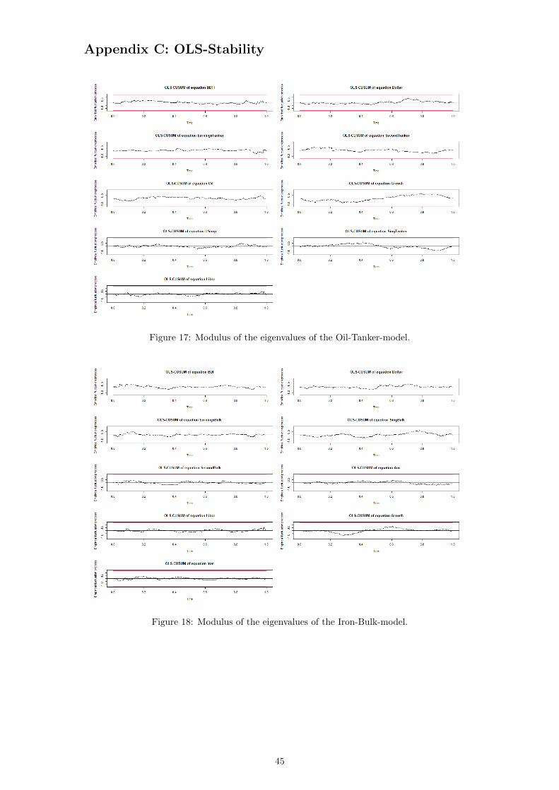
Appendix C: OLS-Stability
Figure 17: Modulus of the eigenvalues of the Oil-Tanker-model.
Figure 18: Modulus of the eigenvalues of the Iron-Bulk-model.
45

Bibliography
Books
Stopford, Martin, Maritime Economics, 3rd ed., Routledge 2 Park Square, Milton Park, Abingdon, Oxon
OX14 4RN, 2009.
Lutkepohl, Helmut, New Introduction to Multiple Time Series Analysis, 1st ed., Springer-Verlag Berlin
Heidelberg 2005
Brockwell, Peter J., Davis, Richard A., Introduction to Time Series and Forecasting, 2nd ed., 2002,
Springer-Verlag New York, Inc.
Reports, Articles, Lecture Notes
UNCTAD, Review of Maritime Transport 2020. New York: United Nations Publications 405 East 42nd
Street New York, NY 10017, 2020. https://unctad.org/system/files/official-document/rmt2020/ en.pdf
(Retrieved 2020-12-01).
UNCTAD,2019 Handbook of Statistics. New York: United Nations Publications 405 East 42nd Street
New York, NY 10017, 2020. https://unctad.org/system/files/official-document/tdstat44/ en.pdf (Re-
trieved 2020-12-01).
Jackson, Mark, Lad, Deepa, Baltic Exchange, Guide to Market Benchmarks, Version 4.1 – March 2020
Baltic Exchange Information Services Ltd.
Vangelis Tsioumas, Stratos Papadimitriou, Yiannis Smirlis, Shaher Zahran Zahran, A Novel Approach
to Forecasting the Bulk Freight Market, The Asian Journal of Shipping and Logistics, Volume 33, Issue
1, 2017, Pages 33-41, ISSN 2092-5212, https://doi.org/10.1016/j.ajsl.2017.03.005.
(http://www.sciencedirect.com/science/article/pii/S2092521217300056)
Nektarios A. Michail, Konstantinos D. Melas, Quantifying the relationship between seaborne trade and
shipping freight rates: A Bayesian vector autoregressive approach, Maritime Transport Research, 2020,
100001, ISSN 2666-822X, https://doi.org/10.1016/j.martra.2020.100001.
(http://www.sciencedirect.com/science/article/pii/S2666822X20300010)
Lutkepohl, Helmut, Vector Autoregressive Models, European University Institute, Department of Eco-
nomics, EUI Working Paper ECO 2011/30, 2011.
Hult, Henrik, Lecture Notes in Statistical Inference, lecture 7, EM-algorithm, KTH Royal Institute of
Technology, Department of Mathematics , 2019, pdf, retrieved 2020-12-01.
Web Pages
Pfaff B, Stiegler M. Package VARS. R-Project.org. Published 2015 Feb 20. Retreived from cran.r-
project.org/web/packages/vars/vars.pdf
Honaker J, King G, Blackwell M. Package Amelia. R-Project.org. Published 2019 Nov 24. Retreived
from cran.r-project.org/web/packages/Amelia/Amelia.pdf
46

Raw Data
Baltic Exchange (2020), Baltic Dirty Tanker Index, 2009-2020, https://www.balticexchange.com/en/index.html,
extracted 2020-12-01.
US Energy Information Administration (2020), Brent Oil Price, 2009-2020,
https://www.eia.gov/dnav/pet/hist/RBRTED.htm, extracted 2020-09-15.
Clarksons World Fleet Register Time Series(2020), Tanker Earnings, 2009-2020,
https://www.clarksons.net/n//wfr/timeseries/advanced/50/1, extracted 2020-09-15
Investing.com (2020), Dollar Index, 2009-2020, https://se.investing.com/currencies/us-dollar-index, ex-
tracted 2020-09-15
Macrotrends (2020), LIBOR 3-month, 2009-2020, https://www.macrotrends.net/2520/3-month-libor-
rate-historical-chart,
Baltic Exchange (2020), Baltic Second Hand Tanker Price, 2009-2020,
https://www.balticexchange.com/en/index.html, extracted 2020-09-15.
Maritime and Port Authority of Singapore(2020), Tanker Arrivals, 2009-2020,
http://www.mpa.gov.sg/web/portal/home/port-of-singapore/port-statistics, extracted 2020-09-15
US Energy Information Administration (2020), Total Crude Imports,
https://www.eia.gov/dnav/pet/pet move impcus a2 nus ep00 im0 mbbl m.htm, extracted 2020-09-15
Clarksons World Fleet Register Time Series(2020), Ship Orderbook, 2009-2020,
https://www.clarksons.net/n//wfr/timeseries/advanced/50/1, extracted 2020-09-15
Baltic Exchange (2020), Baltic Dry Index, 2009-2020, https://www.balticexchange.com/en/index.html,
extracted 2020-12-01.
Investing.com (2020), Iron ore fines 62% Fe CFR, 2009-2020, https://se.investing.com/commodities/iron-
ore-62-cfr-futures, extracted 2020-09-15
Clarksons World Fleet Register Time Series(2020), Bulk Earnings, 2009-2020,
https://www.clarksons.net/n//wfr/timeseries/advanced/50/1, extracted 2020-09-15
Baltic Exchange (2020), Baltic Second Hand Bulk Price, 2009-2020, https://www.balticexchange.com/en/index.html,
extracted 2020-09-15.
Maritime and Port Authority of Singapore(2020), Vessel Arrivals, 2009-2020,
http://www.mpa.gov.sg/web/portal/home/port-of-singapore/port-statistics, extracted 2020-09-15
Australian Bureau of Statistics(2020), Preliminary merchandise exports, standard international trade
classification, 2009-2020, https://www.abs.gov.au/statistics/economy/international-trade/international-
merchandise-trade-preliminary-australia/latest-release, extracted 2020-09-15
47


TRITA -SCI-GRU 2020:384
www.kth.se


![Hexastore: Sextuple Indexing for Semantic Web Data …2.2.2 Multiple-indexing Approaches Harth and Decker [27] proposed storing RDF data based on multiple indices, while taking into](https://img.dokumen.tips/doc/110x75/5ed3ae49c4540779ca664dde/hexastore-sextuple-indexing-for-semantic-web-data-222-multiple-indexing-approaches.jpg)