Multiple Radar Target Tracking in Environments with High ... · Multiple Radar Target Tracking in Environments with High Noise and Clutter by Samuel P. Ebenezer A Dissertation Presented

Multiple Radar Target Tracking in Environments with High Noise and Clutter

by

Samuel P. Ebenezer

A Dissertation Presented in Partial Fulfillmentof the Requirement for the Degree

Doctor of Philosophy

Approved December 2014 by theGraduate Supervisory Committee:

Antonia Papandreou-Suppappola, ChairChaitali Chakrabarti

Daniel BlissNarayan Kovvali

ARIZONA STATE UNIVERSITY

May 2015

ABSTRACT

Tracking a time-varying number of targets is a challenging dynamic state estima-

tion problem whose complexity is intensified under low signal-to-noise ratio (SNR)

or high clutter conditions. This is important, for example, when tracking multiple,

closely spaced targets moving in the same direction such as a convoy of low observable

vehicles moving through a forest or multiple targets moving in a crisscross pattern.

The SNR in these applications is usually low as the reflected signals from the targets

are weak or the noise level is very high. An effective approach for detecting and track-

ing a single target under low SNR conditions is the track-before-detect filter (TBDF)

that uses unthresholded measurements. However, the TBDF has only been used to

track a small fixed number of targets at low SNR.

This work proposes a new multiple target TBDF approach to track a dynami-

cally varying number of targets under the recursive Bayesian framework. For a given

maximum number of targets, the state estimates are obtained by estimating the

joint multiple target posterior probability density function under all possible target

existence combinations. The estimation of the corresponding target existence combi-

nation probabilities and the target existence probabilities are also derived. A feasible

sequential Monte Carlo (SMC) based implementation algorithm is proposed. The

approximation accuracy of the SMC method with a reduced number of particles is

improved by an efficient proposal density function that partitions the multiple target

space into a single target space.

The proposed multiple target TBDF method is extended to track targets in sea

clutter using highly time-varying radar measurements. A generalized likelihood func-

tion for closely spaced multiple targets in compound Gaussian sea clutter is derived

together with the maximum likelihood estimate of the model parameters using an

iterative fixed point algorithm. The TBDF performance is improved by proposing

i

a computationally feasible method to estimate the space-time covariance matrix of

rapidly-varying sea clutter. The method applies the Kronecker product approxima-

tion to the covariance matrix and uses particle filtering to solve the resulting dynamic

state space model formulation.

ii

To my forebearing wife Bernice and my loving daughters Anya and Neha

iii

ACKNOWLEDGEMENTS

I would like to express my utmost gratitude to my advisor Prof.Antonia Papandreou-

Suppappola, for graciously agreeing to be my PhD thesis advisor despite knowing that

this academic process is going to be a part-time endeavor. She made the entire process

stimulating by directing me with challenging research topics. She was also patient

and kind during the arduous journey by nudging me in the right direction to achieve

the end goal even though sometimes it seemed unattainable. I can never forget her

burning the midnight oil many times while writing various research papers pertaining

to this work and teaching me how to write a precise and technically rigorous research

paper. I would also like to thank my committee members, Prof.Chaitali Chakrabarti,

Prof.Daniel Bliss and Dr.Narayan Kovvali for agreeing to be in the committee despite

their busy schedules. I am thankful for their constructive and relevant feedback and

also reviewing this thesis. I am especially grateful to Dr.Narayan Kovvali for many

stimulating and thought provoking discussions that motivated me to approach the

problems in a fundamentally sound manner. I would also like to thank Dr.Seth

Suppappola and Mr.Doug Olsen at Cirrus Logic Inc., for allowing me to embark on

this parallel journey and being flexible during the seemingly never ending process. I

am also thankful to my sister Ms.Geetha Andrew for carefully reviewing this thesis.

I am indebted to my mother for everything she has done for me through all my years.

Finally, none of this would have happened without the constant encouragement and

prayers of my patient wife Bernice and I am blessed to have her at my side.

iv

TABLE OF CONTENTS

Page

LIST OF TABLES . . . . . . . . . . . . . . . . . . . . . . . . . . . . . . . . . . . . . . . . . . . . . . . . . . . . . . . . . xi

LIST OF FIGURES . . . . . . . . . . . . . . . . . . . . . . . . . . . . . . . . . . . . . . . . . . . . . . . . . . . . . . . . xii

CHAPTER

1 INTRODUCTION . . . . . . . . . . . . . . . . . . . . . . . . . . . . . . . . . . . . . . . . . . . . . . . . . . . 1

1.1 Motivation . . . . . . . . . . . . . . . . . . . . . . . . . . . . . . . . . . . . . . . . . . . . . . . . . . . . . 1

1.1.1 Target Tracking . . . . . . . . . . . . . . . . . . . . . . . . . . . . . . . . . . . . . . . . . . 1

1.1.2 Target Tracking in Clutter . . . . . . . . . . . . . . . . . . . . . . . . . . . . . . . . 2

1.1.3 Multiple Target Tracking . . . . . . . . . . . . . . . . . . . . . . . . . . . . . . . . . 4

1.1.4 Track-before-detect Filter . . . . . . . . . . . . . . . . . . . . . . . . . . . . . . . . . 6

1.1.5 Multiple Target Track-before-detect Filtering . . . . . . . . . . . . . . 6

1.2 Summary of Proposed Thesis Work . . . . . . . . . . . . . . . . . . . . . . . . . . . . . . 9

1.2.1 Multiple Mode Multiple Target Track-before-detect Filter . . . 9

1.2.2 Partition Based Proposal Density Function for Multiple Mode

Multiple Target Track-before-detect Filter . . . . . . . . . . . . . . . . . 10

1.2.3 Multiple Target TBDF in Compound Gaussian Sea Clutter . 11

1.2.4 Estimation of Sea Clutter Space-Time Covariance Matrix

Using Kronecker Product Approximation . . . . . . . . . . . . . . . . . . 12

1.3 Thesis Organization . . . . . . . . . . . . . . . . . . . . . . . . . . . . . . . . . . . . . . . . . . . . . 12

2 REVIEW ON TARGET TRACKING . . . . . . . . . . . . . . . . . . . . . . . . . . . . . . . . . 17

2.1 Single Target Tracking . . . . . . . . . . . . . . . . . . . . . . . . . . . . . . . . . . . . . . . . . . 17

2.1.1 State Space Model Formulation . . . . . . . . . . . . . . . . . . . . . . . . . . . 17

2.1.2 Bayesian Filtering Framework. . . . . . . . . . . . . . . . . . . . . . . . . . . . . 18

2.2 Kalman Filtering for Single Target Tracking . . . . . . . . . . . . . . . . . . . . . . 19

2.2.1 Algorithm Description . . . . . . . . . . . . . . . . . . . . . . . . . . . . . . . . . . . . 19

v

CHAPTER Page

2.2.2 Kalman Filter Simulations for Two-dimensional Tracking . . . 21

2.3 Sequential Monte Carlo Methods for Single Target Tracking . . . . . . . 23

2.3.1 Monte Carlo Integration . . . . . . . . . . . . . . . . . . . . . . . . . . . . . . . . . . 24

2.3.2 Importance Sampling . . . . . . . . . . . . . . . . . . . . . . . . . . . . . . . . . . . . 25

2.3.3 Particle Filtering . . . . . . . . . . . . . . . . . . . . . . . . . . . . . . . . . . . . . . . . . 26

2.3.4 Sampling Importance Resampling Filter . . . . . . . . . . . . . . . . . . . 28

2.4 Multiple Target Tracking . . . . . . . . . . . . . . . . . . . . . . . . . . . . . . . . . . . . . . . . 28

2.4.1 State Space Model Formulation . . . . . . . . . . . . . . . . . . . . . . . . . . . 28

2.4.2 Joint Probabilistic Data Association Filter . . . . . . . . . . . . . . . . . 29

2.5 Sequential Monte Carlo Based Joint Probabilistic Data Association . 34

2.5.1 Monte Carlo Based JPDA Filter . . . . . . . . . . . . . . . . . . . . . . . . . . 34

2.5.2 Data Association and Sequential Monte Carlo . . . . . . . . . . . . . . 35

2.5.3 Particle Filter Implementation of MCJPDA . . . . . . . . . . . . . . . . 36

2.5.4 MCJPDA Using SIR particle filter . . . . . . . . . . . . . . . . . . . . . . . . 37

3 SINGLE TARGET SEQUENTIALMONTE CARLO TRACK-BEFORE-

DETECT FILTERING . . . . . . . . . . . . . . . . . . . . . . . . . . . . . . . . . . . . . . . . . . . . . . 40

3.1 Tracking Under Low Signal-to-Noise Ratio Conditions . . . . . . . . . . . . . 40

3.2 Sequential Monte Carlo Track-before-detect Filtering . . . . . . . . . . . . . . 41

3.2.1 State Space Model . . . . . . . . . . . . . . . . . . . . . . . . . . . . . . . . . . . . . . . 41

3.2.2 Bayesian Solution to Track-before-detect Filtering . . . . . . . . . . 42

3.2.3 Particle Filter Implementation of Track-before-detect Filtering 43

3.3 Efficient Particle Filter Based Track-before-detect Filtering . . . . . . . . 45

3.3.1 Algorithm Description . . . . . . . . . . . . . . . . . . . . . . . . . . . . . . . . . . . . 45

3.3.2 Implementation of the Efficient PF-TBDF . . . . . . . . . . . . . . . . . 47

vi

CHAPTER Page

3.4 Target Tracking Example Using Image Measurements . . . . . . . . . . . . . 49

3.4.1 Image Measurement Model . . . . . . . . . . . . . . . . . . . . . . . . . . . . . . . 49

3.4.2 Simulations . . . . . . . . . . . . . . . . . . . . . . . . . . . . . . . . . . . . . . . . . . . . . . 50

3.5 Target Tracking Example Using Radar Measurements . . . . . . . . . . . . . 57

3.5.1 Radar Measurement Model . . . . . . . . . . . . . . . . . . . . . . . . . . . . . . . 57

3.5.2 Simulations Using Rayleigh Measurement Noise . . . . . . . . . . . . 60

3.5.3 Simulations with Measurements in Clutter . . . . . . . . . . . . . . . . . 65

4 MULTIPLE TARGET TRACK-BEFORE-DETECT FILTERING. . . . . . . 68

4.1 Tracking Multiple Targets Under Low Signal-to-Noise Ratio Con-

ditions . . . . . . . . . . . . . . . . . . . . . . . . . . . . . . . . . . . . . . . . . . . . . . . . . . . . . . . . . 68

4.2 Multiple Mode Multiple Target Tracking Model . . . . . . . . . . . . . . . . . . . 69

4.2.1 State Model for Dynamically-varying Number of Targets . . . . 69

4.2.2 Mode Transition Matrix . . . . . . . . . . . . . . . . . . . . . . . . . . . . . . . . . . 72

4.2.3 Measurement Model Using Image Data . . . . . . . . . . . . . . . . . . . . 74

4.2.4 Measurement Model Using Radar Data . . . . . . . . . . . . . . . . . . . . 75

4.3 Multiple Mode Multiple Target Track-before-detect Filtering . . . . . . . 76

4.3.1 Posterior Density for Multiple Mode Multiple Targets . . . . . . 76

4.3.2 Likelihood Function for Image Measurements . . . . . . . . . . . . . . 80

4.3.3 Likelihood Function for Radar Measurements . . . . . . . . . . . . . . 81

4.3.4 Prediction Step of MM-MT-TBDF . . . . . . . . . . . . . . . . . . . . . . . . 81

4.3.5 Joint PDF Mixture Weights Calculation in MM-MT-TBDF . 83

4.3.6 Mode Probability Calculation for the MM-MT-TBDF . . . . . . 84

4.4 Particle Filter Implementation of Multiple Mode Multiple Target

TBDF . . . . . . . . . . . . . . . . . . . . . . . . . . . . . . . . . . . . . . . . . . . . . . . . . . . . . . . . . 87

vii

CHAPTER Page

4.4.1 MM-MT-TBDF Using Sampling Importance Resampling Par-

ticle Filter . . . . . . . . . . . . . . . . . . . . . . . . . . . . . . . . . . . . . . . . . . . . . . . 88

4.5 Simulations . . . . . . . . . . . . . . . . . . . . . . . . . . . . . . . . . . . . . . . . . . . . . . . . . . . . 94

4.5.1 Tracking Three Targets Using Image Measurements . . . . . . . . 94

4.5.2 Tracking Three Targets Using Radar Measurements . . . . . . . . 96

5 Efficient Implementation of Multiple Target Track-before-detect Filtering 101

5.1 Computational Issues of the Multiple Mode Multiple Target Track-

before-detect Filter . . . . . . . . . . . . . . . . . . . . . . . . . . . . . . . . . . . . . . . . . . . . . 101

5.2 Proposal Function Using PF Partition Method . . . . . . . . . . . . . . . . . . . . 102

5.3 MM-MT-TBDF-IP with Markov Chain Monte Carlo . . . . . . . . . . . . . . 106

5.4 Simulations . . . . . . . . . . . . . . . . . . . . . . . . . . . . . . . . . . . . . . . . . . . . . . . . . . . . 108

5.4.1 Tracking Three Targets Using Radar Measurements . . . . . . . . 108

5.4.2 Comparison of Different PF Schemes . . . . . . . . . . . . . . . . . . . . . . 111

5.4.3 Effects of Intensity Modeling Error Variance . . . . . . . . . . . . . . . 111

5.4.4 Effects of Spreading Factors . . . . . . . . . . . . . . . . . . . . . . . . . . . . . . 112

5.4.5 Peak SNR Analysis . . . . . . . . . . . . . . . . . . . . . . . . . . . . . . . . . . . . . . 115

5.4.6 Closely Moving Targets Tracking Analysis . . . . . . . . . . . . . . . . . 116

5.4.7 Six Targets Tracking Analysis . . . . . . . . . . . . . . . . . . . . . . . . . . . . . 118

5.4.8 Performance Comparison Between PHDF-TBDF and MM-

MT-TBDF-IP-MCMC. . . . . . . . . . . . . . . . . . . . . . . . . . . . . . . . . . . . 121

5.5 Computational Complexity Analysis . . . . . . . . . . . . . . . . . . . . . . . . . . . . . 123

5.5.1 Heuristic Decision-directed Approaches . . . . . . . . . . . . . . . . . . . . 123

5.5.2 Effects of Particle Filter Size . . . . . . . . . . . . . . . . . . . . . . . . . . . . . . 126

viii

CHAPTER Page

6 TRACK-BEFORE-DETECT FILTERING OF MULTIPLE TARGETS

IN SEA CLUTTER. . . . . . . . . . . . . . . . . . . . . . . . . . . . . . . . . . . . . . . . . . . . . . . . . . 127

6.1 Target Tracking in Sea Clutter . . . . . . . . . . . . . . . . . . . . . . . . . . . . . . . . . . . 127

6.2 Measurement from Pulse Doppler Radar with Clutter . . . . . . . . . . . . . 130

6.3 Compound Gaussian Clutter Model . . . . . . . . . . . . . . . . . . . . . . . . . . . . . . 134

6.3.1 Factors Affecting Statistical Sea Clutter Modeling . . . . . . . . . . 134

6.3.2 Speckle and Texture Sea Clutter Components . . . . . . . . . . . . . . 136

6.3.3 Doppler Model for Sea Clutter . . . . . . . . . . . . . . . . . . . . . . . . . . . . 138

6.4 Likelihood Function in Complex Gaussian Clutter . . . . . . . . . . . . . . . . . 139

6.5 Likelihood Function in Compound Gaussian Clutter . . . . . . . . . . . . . . . 142

6.5.1 Asymptotic Generalized Likelihood Function . . . . . . . . . . . . . . . 142

6.5.2 Adaptive Generalized Likelihood Function Based on Kelly’s

Method . . . . . . . . . . . . . . . . . . . . . . . . . . . . . . . . . . . . . . . . . . . . . . . . . 144

6.5.3 Maximum Likelihood Estimation of Clutter Statistics . . . . . . . 146

6.5.4 Calculation of Generalized Likelihood Ratio . . . . . . . . . . . . . . . . 148

6.5.5 Fixed Point Algorithm for ML Estimation of Clutter Statistics150

6.5.6 Relation Between Test Statistics . . . . . . . . . . . . . . . . . . . . . . . . . . 152

6.6 Track-before-detect Filtering Framework in Clutter . . . . . . . . . . . . . . . . 153

6.7 Simulations . . . . . . . . . . . . . . . . . . . . . . . . . . . . . . . . . . . . . . . . . . . . . . . . . . . . 154

6.7.1 Low Resolution Radar and Complex Gaussian Clutter . . . . . . 154

6.7.2 High Resolution Radar and Compound Gaussian Clutter . . . 159

7 ESTIMATIONOF RAPIDLY-VARYING SEA CLUTTER USING NEAR-

EST KRONECKER PRODUCT APPROXIMATION . . . . . . . . . . . . . . . . . . 165

7.1 Rapidly-varying Sea Clutter Characterization . . . . . . . . . . . . . . . . . . . . . 165

ix

CHAPTER Page

7.2 Rapidly-varying Sea Clutter Model . . . . . . . . . . . . . . . . . . . . . . . . . . . . . . . 167

7.2.1 Measurement Model . . . . . . . . . . . . . . . . . . . . . . . . . . . . . . . . . . . . . . 167

7.2.2 Measurement State Space Model . . . . . . . . . . . . . . . . . . . . . . . . . . 169

7.2.3 Clutter Covariance Matrix State Space Model . . . . . . . . . . . . . . 172

7.2.4 Covariance Nearest Kronecker Product Approximation. . . . . . 173

7.3 Validation of KP Approximation Using Real Sea Clutter Measure-

ment . . . . . . . . . . . . . . . . . . . . . . . . . . . . . . . . . . . . . . . . . . . . . . . . . . . . . . . . . . . 177

7.4 Covariance Matrix Estimation Using Sequential Monte Carlo Tech-

nique . . . . . . . . . . . . . . . . . . . . . . . . . . . . . . . . . . . . . . . . . . . . . . . . . . . . . . . . . . 179

7.4.1 Estimation Approach . . . . . . . . . . . . . . . . . . . . . . . . . . . . . . . . . . . . . 179

7.4.2 Simulations . . . . . . . . . . . . . . . . . . . . . . . . . . . . . . . . . . . . . . . . . . . . . . 181

7.5 Track-before-detect Filtering in Sea Clutter . . . . . . . . . . . . . . . . . . . . . . . 182

7.5.1 Track-before-detect Filtering Formulation with Clutter . . . . . 182

7.5.2 Simulations . . . . . . . . . . . . . . . . . . . . . . . . . . . . . . . . . . . . . . . . . . . . . . 187

8 CONCLUSION AND FUTURE WORK . . . . . . . . . . . . . . . . . . . . . . . . . . . . . . . 194

8.1 Conclusion . . . . . . . . . . . . . . . . . . . . . . . . . . . . . . . . . . . . . . . . . . . . . . . . . . . . . 194

8.2 Future Work . . . . . . . . . . . . . . . . . . . . . . . . . . . . . . . . . . . . . . . . . . . . . . . . . . . 197

REFERENCES . . . . . . . . . . . . . . . . . . . . . . . . . . . . . . . . . . . . . . . . . . . . . . . . . . . . . . . . . . . . 198

APPENDIX

A PROPERTIES OF KRONECKER PRODUCT . . . . . . . . . . . . . . . . . . . . . . . . 212

x

LIST OF TABLES

Table Page

1.1 List of Acronyms . . . . . . . . . . . . . . . . . . . . . . . . . . . . . . . . . . . . . . . . . . . . . . . . . . 14

3.1 Simulated Pulse-Doppler Radar System Parameters . . . . . . . . . . . . . . . . . . 62

4.1 Target Presence Indicator Values for L =2 Targets (M =4 Modes). . . . 70

4.2 True Target Combination at Different Time Steps . . . . . . . . . . . . . . . . . . . . 98

6.1 Test Statistics for Complex Gaussian and Compound Gaussian Clutter

with Random and Deterministic Texture Component . . . . . . . . . . . . . . . . . 155

6.2 Simulated Low Resolution Radar System Parameters . . . . . . . . . . . . . . . . . 156

6.3 Simulated High Resolution Radar System Parameters . . . . . . . . . . . . . . . . 160

xi

LIST OF FIGURES

Figure Page

2.1 True and Estimated Target Trajectory (Top); Velocity in the y-direction

(Bottom Right); and Velocity in the x-direction (Bottom Left). In the

Top Plot, the Measurements are Represented by Crosses. . . . . . . . . . . . . . 23

2.2 True and Estimated Trajectories for Four Targets (Top); Velocity in the

y-direction (Bottom Right); and Velocity in the x-direction (Bottom

Left). The Top Plot Also Shows the Target and Clutter Associated

Measurements Represented by Circles and Crosses, respectively. . . . . . . . 32

2.3 Tracking Performance of JPDA Filter for Various Values of Clutter

Density, Number of Targets and Probability of Detection: RMSE at

0.5 Clutters Per Measurement Time with L = 3 Targets (Top Left);

RMSE at 3 Clutters Per Measurement Time with L = 3 Targets

(Top Right); RMSE at 3 Clutters Per Measurement Time with L = 4

Targets (Bottom Right); and RMSE at 0.5 Clutters Per Measurement

Time with L = 4 Targets (Bottom Left). . . . . . . . . . . . . . . . . . . . . . . . . . . . . 33

2.4 MCJPDA Filter Performance: True and Estimated Trajectories for

Four Targets (Top Left); Target and Clutter Associated Measurements

(Top Right, Green and Black Stars Represent Target and Clutter As-

sociated Range Measurements, respectively, and Red and Cyan Dots

Represent Target and Clutter Associated Range-Rate Measurements,

respectively); Velocity in the y-direction (Bottom Right); and Velocity

in the x-direction (Bottom Left). . . . . . . . . . . . . . . . . . . . . . . . . . . . . . . . . . . . . 39

3.1 Measurement Frame at Different Time Steps at 20 dB Peak SNR. In

all the Plots, the x and y Axes Correspond to the x and y Coordinates

in the FOV, respectively. . . . . . . . . . . . . . . . . . . . . . . . . . . . . . . . . . . . . . . . . . . . 51

xii

Figure Page

3.2 Measurement Frame at Different Time Steps at 6 dB Peak SNR. . . . . . . 52

3.3 Target Existence Probability at 6 dB Peak SNR (Red Stars Represent

the Time Steps at which the Target Truly Exist). . . . . . . . . . . . . . . . . . . . . 53

3.4 Particle Distribution for Target Position (Top 6 Plots, where the x and

y Axes Represent the x and y Coordinates in the FOV, respectively);

Histogram of Target Intensity Estimate at Different Frames (Bottom

6 Plots, where the x and y Axes Represent Intensity and Number of

Particles with the Corresponding Intensity Value, respectively). . . . . . . . 54

3.5 Target Position Estimates, x Coordinate (Top Left); and y Coordinate

(Top Right). True and Estimated Target Trajectory at 6 dB Peak SNR

(Bottom). . . . . . . . . . . . . . . . . . . . . . . . . . . . . . . . . . . . . . . . . . . . . . . . . . . . . . . . . 55

3.6 Target Existence Probability for the Original PF-TBDF and the Effi-

cient PF-TBDF Methods (a) SNR = 12 dB; (b) SNR = 6 dB; and (c)

SNR = 3 dB. . . . . . . . . . . . . . . . . . . . . . . . . . . . . . . . . . . . . . . . . . . . . . . . . . . . . . . 56

3.7 Position RMSE for the Original PF-TBDF and the Efficient PF-TBDF

Methods (a) SNR = 12 dB; (b) SNR = 6 dB; and (c) SNR = 3 dB. . . . 57

3.8 Range and Range-Rate Processing of a Pulse-Doppler Radar System. . . 59

3.9 Signal Condition at Various Points in the Radar System at 15 dB

Peak SNR: Raw Received Signal (Top Left); Matched Filter Output

(Top Right); Noise-Free Range and Range-Rate Measurement (Bottom

Right); and Noisy Range and Range-Rate Measurement (Bottom Left). 61

3.10 Measurement Frame with Rayleigh Noise at Different Time Steps at

15 dB Peak SNR. In all the Plots, the x, y and z Axes Correspond to

Range in m, Range-Rate in m/s, and Intensity, respectively. . . . . . . . . . . . 63

xiii

Figure Page

3.11 Particle Distribution for Target Position at 15 dB Peak SNR (Top 6

Plots, where the x and y Axes Represent the x and y Coordinates in

the FOV, respectively); and Histogram of Target Intensity Estimate at

Different Frames (Bottom 6 Plots, where the x and y Axes Represent

Intensity and Number of Particles with the Corresponding Intensity

Value, respectively). . . . . . . . . . . . . . . . . . . . . . . . . . . . . . . . . . . . . . . . . . . . . . . . . 64

3.12 Target Position Estimates, x Coordinate (Top Left); y Coordinate (Top

Right). True and Estimated Target Trajectory at 15 dB Peak SNR

(Bottom). . . . . . . . . . . . . . . . . . . . . . . . . . . . . . . . . . . . . . . . . . . . . . . . . . . . . . . . . . 65

3.13 Target Existence Probability for Different Peak SNR Values and Clut-

ter Densities. . . . . . . . . . . . . . . . . . . . . . . . . . . . . . . . . . . . . . . . . . . . . . . . . . . . . . . 66

3.14 True and Estimated Target Trajectory: (a) SNR = 18 dB, 10 Clutter

Measurements Per Dwell; and (b) SNR = 15 dB, 5 Clutter Measure-

ments Per Dwell. . . . . . . . . . . . . . . . . . . . . . . . . . . . . . . . . . . . . . . . . . . . . . . . . . . . 67

4.1 MM-MT-TBDF Algorithm Block Diagram for Multiple Target Tracking. 86

4.2 Illustration of MM-MT-TBDF Algorithm for L = 2 Targets Show-

ing the Dominant Probabilities and the Relevant Posterior PDFs for

Different Mode Transitions. . . . . . . . . . . . . . . . . . . . . . . . . . . . . . . . . . . . . . . . . . 87

4.3 Measurement Frames: (a) Time Step 15, 19.8 dB Peak SNR. (b) Time

Step 15, 10.2 dB Peak SNR . . . . . . . . . . . . . . . . . . . . . . . . . . . . . . . . . . . . . . . . . 96

4.4 Image Measurement Case: (a) Target Existence Probability (Red Cir-

cles, Blue Stars and Black Triangles Indicate the Frames at which

Target 1, Target 2 and Target 3 Truly Exist, respectively); and (b)

Tracking Error at Different SNR Conditions, OSPA(40,2). . . . . . . . . . . . . 97

xiv

Figure Page

4.5 Mode Probability for Three Targets at 3 dB Peak SNR. . . . . . . . . . . . . . . 99

4.6 Radar Measurement Tracking of Three Targets at 3 dB Peak SNR:

(a) True and Estimated Target Trajectories (Solid Lines Represent the

True Target Trajectory and Red Circles, Blue Stars and Black Triangles

Represent the Estimated Trajectory of Target 1, Target 2 and Target

3 respectively; and (b) Tracking Error, OSPA(16,2). . . . . . . . . . . . . . . . . . . 100

5.1 Mode Probability for Three Targets at 3 dB Peak SNR (MM-MT-

TBDF-IP-MCMC). . . . . . . . . . . . . . . . . . . . . . . . . . . . . . . . . . . . . . . . . . . . . . . . . 108

5.2 True and Estimated Target Trajectories for Three Targets at 3 dB Peak

SNR. . . . . . . . . . . . . . . . . . . . . . . . . . . . . . . . . . . . . . . . . . . . . . . . . . . . . . . . . . . . . . 109

5.3 OSPA(40,2) for Three Targets at 3 dB Peak SNR. . . . . . . . . . . . . . . . . . . . . 110

5.4 OSPA Vs Process Model Variance. . . . . . . . . . . . . . . . . . . . . . . . . . . . . . . . . . . 112

5.5 Effects of Intensity Modeling Error Variance: (a) Instantaneous Peak

SNR for Target 1; and (b) OSPA Versus Time for Various Values of q2. 113

5.6 Effects of Spreading Factors: (a) OSPA Versus Time for Various Spread-

ing Factors; and (b) Probability of Target Existence Computed Using

Equation (4.29), Red: Target 1, Blue: Target 2, Black: Target 3. . . . . . . 114

5.7 Mode Probability Computed Using Equation (4.19) For Three Targets

Case, Solid: σr = 0.509, σr = 0.077, σθ = 0.033 (1σ), Dashed: σr =

0.764, σr = 0.116, σθ = 0.049 (1.5σ). . . . . . . . . . . . . . . . . . . . . . . . . . . . . . . . . . 115

5.8 Averaged OSPA Vs. Peak SNRs. . . . . . . . . . . . . . . . . . . . . . . . . . . . . . . . . . . . . 116

5.9 Closely-Moving Targets Case: (a) Trajectory of Targets Moving in

Opposite Direction; and (b) Trajectory of Targets Moving in Same

Direction. . . . . . . . . . . . . . . . . . . . . . . . . . . . . . . . . . . . . . . . . . . . . . . . . . . . . . . . . . 117

xv

Figure Page

5.10 Closely-Moving Targets Case: (a) Euclidean Distance Between 3 Closely-

Moving Targets (Crosses Represent Targets Moving in Opposite Direc-

tions); and (b) Tracking Error, OSPA(16, 2). . . . . . . . . . . . . . . . . . . . . . . . . . 118

5.11 Particle Distribution for Tracking Six Targets Case with L =5 Targets.119

5.12 True and Estimated Trajectories for Tracking Six Targets Case with

L =5 Targets. . . . . . . . . . . . . . . . . . . . . . . . . . . . . . . . . . . . . . . . . . . . . . . . . . . . . 120

5.13 Image Measurement Case: (a) OSPA at Different Peak SNR (19.8 dB,

16.3 dB, 13.8 dB); and (b) OSPA at 10.2 dB Peak SNR. . . . . . . . . . . . . . . 121

5.14 Probability of Target Existence. . . . . . . . . . . . . . . . . . . . . . . . . . . . . . . . . . . . . . 122

5.15 Computational Analysis: (a) Processing Time Difference Between all

Modes and Mode Probability Selected Modes; and (b) OSPA Difference

Between all Modes and Mode Probability Selected Modes. . . . . . . . . . . . . 123

5.16 Average and Peak Processing Time for Different Maximum Number of

Targets. . . . . . . . . . . . . . . . . . . . . . . . . . . . . . . . . . . . . . . . . . . . . . . . . . . . . . . . . . . . 125

5.17 Effects of Partilce Filter Size for L = 3 Targets: (a) Tracking Error;

and (b) Average and Peak Processing Time. . . . . . . . . . . . . . . . . . . . . . . . . . 126

6.1 (A) Target Trajectory in the x Coordinate; and (b) Target Trajectory

in the y Coordinate. . . . . . . . . . . . . . . . . . . . . . . . . . . . . . . . . . . . . . . . . . . . . . . . . 157

6.2 (A) Absolute Value of Measurement Dwells at 0 dB SCR. (b) Tracking

Error, OSPA(4000,2). . . . . . . . . . . . . . . . . . . . . . . . . . . . . . . . . . . . . . . . . . . . . . . 158

6.3 Averaged Doppler Spectrum for Different Values of cg. . . . . . . . . . . . . . . . . 161

6.4 Fast Time Measurement, SCR=3 dB: (a) cg=10;(b) cg=0.5; (c) cg=0.2. 163

6.5 Tracking Error for Different Values of cg and SCR = 3 dB. . . . . . . . . . . . . 164

6.6 Tracking Error for Different Values of SCR and cg =0.5. . . . . . . . . . . . . . . 164

xvi

Figure Page

7.1 Sea Clutter Covariance Transition Model for the Matrix in Equation

(7.6). . . . . . . . . . . . . . . . . . . . . . . . . . . . . . . . . . . . . . . . . . . . . . . . . . . . . . . . . . . . . . 173

7.2 (a) Singular Value of the Permuted Covariance Matrix. (b) NKPA

Error for Different Number of Dwells for Estimating the Sample Co-

variance Matrix. . . . . . . . . . . . . . . . . . . . . . . . . . . . . . . . . . . . . . . . . . . . . . . . . . . . 178

7.3 Sea Clutter Covariance Matrix: (a) Dwell 5; and (b) Dwell 40. . . . . . . . . 182

7.4 Covariance Matrix Estimation (Frobenius) Error . . . . . . . . . . . . . . . . . . . . . 183

7.5 Illustration of Extracting a Principal Submatrix. . . . . . . . . . . . . . . . . . . . . . 185

7.6 Pulse Doppler Radar Measurements: (a) SCR = 9dB; (b) SCR = 6

dB; and (c) SCR = 3 dB. . . . . . . . . . . . . . . . . . . . . . . . . . . . . . . . . . . . . . . . . . . . 188

7.7 Cross-Correlation of the Baseband Signal. . . . . . . . . . . . . . . . . . . . . . . . . . . . 188

7.8 (a) Probability of Target Existence; and (b) Tracking Error for Varying

SCR: True and Assumed KP Models (Solid), and Assumed KP Model

Only (Dash). . . . . . . . . . . . . . . . . . . . . . . . . . . . . . . . . . . . . . . . . . . . . . . . . . . . . . . 190

7.9 (a) Probability of Target Existence; and (b) Tracking Error for Varying

SCR: KP (Solid) and CG-LQ (Dash). . . . . . . . . . . . . . . . . . . . . . . . . . . . . . . . 190

7.10 (a) Real Sea Clutter Embedded with Synthetic Target at 12 dB SCR;

and (b) Probability of Target Existence Probability Comparison with

Real Sea Clutter: KP (Solid) and CG-LQ (Dash). . . . . . . . . . . . . . . . . . . . . 191

7.11 Tracking Error Comparison with Real Sea Clutter: (a) SCR=12 dB;

(b) SCR = 9 dB; and (c) SCR = 6 dB. . . . . . . . . . . . . . . . . . . . . . . . . . . . . . . 193

xvii

Chapter 1

INTRODUCTION

1.1 Motivation

The development of radar tracking systems for defense applications started as early

as 1930 and became an active research topic with the development of the Kalman

filter (KF) in 1960 [1]. Initially, the research was primarily focused on target track-

ing for air and maritime defense and guidance radar systems. With new advance-

ments in computational and embedded processing capabilities, radar technology is

now penetrating into many other areas such as air-traffic control for commercial air

travel, weather surveillance radar for locating precipitation [2], vehicle collision avoid-

ance radar systems [3], talker tracking in speech processing [4], image processing [5],

robotics [6], remote sensing [7], and biomedical research [8]. All these diverse appli-

cations are driving the need to improve the robustness of target tracking algorithms

under various environmental conditions.

1.1.1 Target Tracking

Historically, Bayesian techniques have been used to track targets in noise following

the state space model formulation [9]. The KF provides an optimal state parameter

estimate for linear state space models in which the measurement and modeling error

random processes are assumed Gaussian [10]. The alpha-beta filter is a computa-

tionally simple derivative of the KF that was successfully used to estimate a moving

target’s position and velocity [11–13]. Since the KF is optimal only for linear and

Gaussian state space models, the tracking performance of the KF and the alpha-beta

1

filters is not optimal for nonlinear and non-Gaussian models. With the extended KF

(EKF), the state transition and observation models do not need to be linear func-

tions of the target state but, differentiable, so that they can be linearized at the

current estimate using Taylor series approximations [14]. A new class of simulation

based algorithms including the particle filter (PF) or sequential Monte Carlo (SMC)

methods [15–17] have evolved in the late 1990s that can be used for nonlinear and

non-Gaussian distributed state space models.

1.1.2 Target Tracking in Clutter

Target tracking is a complex problem that requires the consideration of many sig-

nal and environmental conditions for practical solutions [9, 18, 19]. For example, the

typical reflected radar signal level from a low observable target is very low. Under low

signal-to-noise ratio (SNR) conditions, it is possible to miss detecting valid measure-

ments originating from existing targets. However, a tracking system should still be

able to estimate the target’s state parameters when a measurement that originated

from a true target is weak. False alarms such as clutter, which are common in real

systems, can further complicate processing. The clutter in a realistic measurement

space can cause uncertainty in the origin of the measurement. This is a data asso-

ciation problem as the uncertainty makes it difficult to associate the measurement

corresponding to the true target. The measurement origin uncertainty is further in-

creased by the presence of multiple targets. In this scenario, it is imperative that

measurements from all possible targets are associated with the corresponding targets

in addition to pruning the measurements originated from clutter. Furthermore, in

many real-life practical cases, the number of targets that are present in the measure-

ment space of a tracking system is not known a priori. Thus, a target tracking system

should not only be able to track the trajectory of moving targets but also estimate

2

the number of targets that are present at each time step. Moreover, the number of

measurements is usually not the same as the number of targets that are present in

the field of view (FOV). In addition to these problems, at each time step, a tracker

must also determine if a particular target has left the FOV and if a new target has

entered the FOV.

The tracking performance of the classical detect-before-track algorithms is accept-

able when tracking a single target in high SNR. However, these algorithms do not

perform well under low SNR conditions or when the measurements also originate from

clutter. At each time step, multiple measurements are available, and the tracker must

identify the measurement associated with the target from all the measurements. In

real-life target tracking applications, the source of a measurement is usually not known

by a tracking system. Hence, the tracker needs to first associate each measurement

with its corresponding source. This data association process is a very critical step in

a practical target tracking system and as a result, many data association techniques

have been proposed in the literature [18, 20]. One of the simplest data association

techniques is the nearest neighbour method, which selects the measurement closest to

the predicted track to update the target state [21]. Even if the state space model is

assumed linear and Gaussian, the estimated target states are not optimal because the

selected measurement need not originate from a target. Track and split is an optimal

data association technique in which all measurements are assumed to be valid and

a new track is initiated for every measurement [22]. However, as the computational

complexity of this technique increases very fast with time because of the exponential

growth of the tree structure, it is not feasible for real-time applications. A probability

based method to track a target in clutter was proposed in [23]. In this probabilistic

data association (PDA) method, the target states for all the measurements are es-

timated separately in addition to computing the measurement-to-target association

3

probability. The approach estimates the final target state by combining all the pos-

sible target states weighted by the corresponding measurement-to-target association

probability [20, 24, 25]. A PF based method to track a target in clutter was also

proposed in [26] for nonlinear/non-Gaussian state space models.

1.1.3 Multiple Target Tracking

The aforementioned tracking problem in clutter becomes extremely complicated

when there is a multiple number of targets to track simultaneously. A comprehen-

sive list of different multiple target tracking techniques together with a comparison

of their performance and computational complexity is presented in [27]. Multiple hy-

pothesis tracking (MHT) [28], [29] is a popular multiple target measurement oriented

technique in which each established target or a new target that gives rise to a measure-

ment sequence is obtained. This technique is similar to the track and split technique

used for single target tracking in clutter. Using the MHT, different possible track

hypotheses are generated when a new measurement set is received. The hypothesis

tracking enables the tracking system to detect when a new target enters or a target

leaves the FOV. The target states for each hypothesis are estimated using a KF, EKF

or PF tracker, depending on the state space model assumptions. The probability of

occurrence of each track hypothesis is computed and their probabilities are used to

compute the weighted average estimate of a target state. Since this algorithm main-

tains the track hypothesis based on the current and past measurements, the validated

target states are available only after some delay. The computational complexity of

this algorithm can grow exponentially as the number of track hypotheses increases.

One could use hypothesis reduction techniques such as zero scan clustering or hypoth-

esis elimination to increase the computational feasibility of this algorithm. The joint

probabilistic data association (JPDA) filter [30] is another popular algorithm that

4

extends the PDA filter for multiple target tracking. This is a zero scan algorithm in

which all the current measurement sets are combined immediately to provide a target

state estimate. In the JPDA filter, given all the measurement data and a known

number of targets, all possible measurement-to-target combinations (hypothesis) are

formed. The state vectors corresponding to all targets are estimated for each hypoth-

esis along with their hypothesis probabilities. Finally, the target state estimates are

combined to obtain the final target estimate. One of the drawbacks of the JPDA filter

is that it assumes that the number of targets present in the measurement space is

known. Hence, this algorithm cannot be used when the number of targets in the FOV

is time-varying. When the JPDA algorithm was originally proposed, it used the KF

to estimate the target state under different hypotheses. In the early 2000s, the JPDA

was often integrated with the PF to track multiple targets for nonlinear/non-Gaussian

state space models [31–34].

Recently, the optimal Bayesian multiple target probability density function (PDF)

estimation approach was proposed using random finite set (RFS) statistics [35–37].

This approach keeps track of the varying number of targets to estimate their state

vectors. However, a feasible implementation of the optimal Bayesian multiple target

PDF estimation does not exist in the literature. Nevertheless, two popular approxima-

tion techniques with feasible implementations have been proposed that approximate

the multiple target PDF by either Poisson [38, 39] or multiple Bernoulli distributions

[36, 40]. The probability hypothesis density filter (PHDF) [38, 39] that approxi-

mates the multiple target PDF by a Poisson distribution has gained popularity in

tracking a varying number of targets with a non-zero probability of detection in the

presence of clutter. The PHDF recursively tracks the intensity function of a Poisson

process that models the number of existing targets in any given range of the single

target state space. In the multiple Bernoulli filtering approach, the posterior PDF

5

is approximated by a multiple Bernoulli distribution and the parameters of this dis-

tribution are updated in each time step [36, 40]. The PHDF can be implemented

using closed form versions by approximating the posterior intensity function by a

Gaussian mixture model under linear and Gaussian assumption for the target motion

and measurement models [41–43]. The SMC version of the PHDF for nonlinear and

non-Gaussian models was originally proposed in [37, 44].

1.1.4 Track-before-detect Filter

In conventional radar systems, tracking moving targets in low SNR using constant

false alarm rate (CFAR) detectors [45, 46] can result in poor performance. Since the

detection threshold for a CFAR detector dynamically increases under low SNR con-

ditions, the probability of target detection is low for a target with small radar cross

section [47]. If the threshold is raised to increase the probability of detection, then

more measurements are needed as input to a tracking algorithm due to the increased

number of false alarms. This increased number of measurements can exponentially

increase the computational complexity of multiple target tracking algorithms such as

JPDA and MHT. To improve the tracking performance under low SNR conditions,

the track-before-detect filter (TBDF) method was proposed that uses unthresholded

measurements. TBDF algorithms based on the Hough transform [48], dynamic pro-

gramming [49] or maximum likelihood methods [50] are generally computationally

intensive [17]. With recent advancement in SMC techniques, TBDF algorithms im-

plemented using PF are now computationally feasible [51–56].

1.1.5 Multiple Target Track-before-detect Filtering

Tracking multiple targets under low SNR or high clutter conditions is a difficult

problem. For example, in maritime surveillance applications, it is critical to track

6

small-sized intruder boats under turbulent sea conditions or in an early warning de-

fense system, it is imperative to detect targets farther away from the radar system.

In these applications, the SNR is usually low as the reflected signal from the target is

weak or the noise level is very high. Tracking multiple targets in such poor conditions

is an extremely challenging problem since the tracking problem is complicated by

many factors such as measurement origin uncertainty, unknown number of targets,

and computational feasibility.

Different TBDF algorithms were considered for tracking a time-varying/fixed num-

ber of multiple targets under varying conditions. The single target PF based TBDF

in [51] was extended to track two targets in [57] by replacing the binary state target

existence variable with a three state mode variable. The particles corresponding to

this mode variable is also propagated during the tracking process and the method was

illustrated using a restrictive example by tracking a second target that spawns from

the first target [57]. Moreover, in this method the target state vector dimension is set

to the maximum number of targets and the state vector dimension is not accounted

for varying number of targets. In addition, this method does not entirely cover all

possible target death and birth combinations. For example, there is no unambiguous

mechanism to track the trajectory of the remaining target after one of the target has

disappeared. The authors in [58] have used the single target TBDF in [51] to track

multiple targets by keeping track of the number of peaks in the estimated posterior

PDF. The authors have exploited the fact that the likelihood function is typically

high in the vicinity of different target’s state vector and this will cause the estimated

posterior PDF to become a multi-modal distribution function with each peak corre-

sponding to different targets. A separate clustering method was used to associate the

particle clusters with different targets. However, clustering based methods can lead

to inaccurate estimates when the number of clusters exceeds the actual number of

7

targets. Moreover, the joint multi-target state PDF is also not estimated, instead a

multi-modal PDF in single target space is estimated. A generalized likelihood ratio

test based multi-target TBDF and a multi-hypothesis test strategy for a known and

unknown number of targets, respectively, were presented in [59]. These methods were

demonstrated for two targets at medium range SNR conditions (8-24 dB). A multi-

target acoustic source tracking TBDF for two known fixed targets was discussed in

[60]. Multiple speech sources were tracked in [61] by detecting and removing each

source with a likelihood ratio computed from particle weights from microphone pair

phase differences. Multi-target TBDF for a passive radar was used in [62] by ex-

tending the single target recursive TBDF to each range-Doppler bin with a target

existence probability and PDF conditioned on target existence in each bin.

The RFS based methods were originally introduced for detect-before-track appli-

cations and they are expected to perform poorly under low SNR/SCR conditions. For

example, the multiple Bernoulli approximation is acceptable only when the clutter

rate is low since it introduces cardinality bias in high clutter situations [63]. More-

over, the SMC implementations of PHDF based multiple target tracking methods

[37, 44, 64, 65] to support non-linear/non-Gaussian models, require a clustering step

to estimate the number of existing targets. Many PHDF based TBDF (PHDF-TBD)

methods for non-linear measurement models exist in literature. A SMC based PHDF-

TBD for image applications was introduced in [66] and demonstrated by tracking three

targets. In [67], the poor performance of one such PHDF-TBD was reported when

tracking three well-separated targets and the performance was improved by using

measurements from multiple sensors. In [68, 69], the PHDF-TBD was used to track

two targets using range, Doppler and bearing angle measurements. An improved

PHDF-TBD was also used in [70] following the multiple model PHDF [71] to track

three maneuvering targets. In the SNR-PHDF [72], the SNR is also tracked and a

8

detection step is included in the tracking method by using the measurement only if

the estimated SNR exceeds certain threshold. The mathematical equivalence of the

SNR-PHDF with the threshold set to zero and the single target TBDF [51] is shown

in [73]. All these SMC based methods require the clustering step. Moreover, in all the

above mentioned RFS based methods, track management is an additional required

step, since the target state estimates from these methods are not distinguishable from

each other. Only recently, a new subset of RFS approach called as labeled multiple

Bernoulli filter [74] are beginning to emerge to accommodate target tracks under low

SNR conditions. A multiple Bernoulli based TBDF with a separate label based track

management step was proposed in [75] and illustrated using image measurement to

track up to 4 targets under high SNR conditions. A multi-target label based RFS

TBDF implemented using SMC method was proposed in [63] and illustrated using

3-D radar (range, Doppler, azimuth) measurement at 10 and 13 dB SNR to track up

to 4 targets.

Most of the aforementioned techniques are implemented using SMC methods, and

they do not track the multiple target PDF. Moreover, many of the RFS based methods

require a separate track management step since they do not associate the estimates

with the target identity. Therefore, the problem of tracking a time-varying number of

multiple targets under severe conditions of low SNR and high clutter is still an active

research topic.

1.2 Summary of Proposed Thesis Work

1.2.1 Multiple Mode Multiple Target Track-before-detect Filter

We propose a multiple target TBDF method to track a varying number of tar-

gets by estimating the target states under all possible target existence combinations

9

[76, 77]. We derive a set of multiple target joint posterior PDFs corresponding to

all possible target existence combinations under the recursive Bayesian framework.

The track management of multiple targets is achieved by tracking all possible target

existence combinations in which the identity of targets are dynamically maintained

as the targets enter and leave the FOV. We propose a feasible implementation of the

algorithm using SMC techniques through three layers of particle filter sets. Thus, the

proposed algorithm is developed by integrating three main concepts: (i) estimating

the PDF of target states under multiple hypotheses [29] in order to consider all pos-

sible target existence combinations at each time step; (ii) multiple particle filtering

[78] in order to have multiple PFs for each hypothesis and then optimally combining

each PF output, weighted by a posterior transition probability; and (iii) a parallel

PF architecture [79] in order to attack the computational complexity problem using

distributed processing.

1.2.2 Partition Based Proposal Density Function for Multiple Mode Multiple

Target Track-before-detect Filter

In general, the number of particles necessary to accurately estimate the target

state vector can grow exponentially as a function of the state vector dimension [80].

Therefore, the proposed SMC implementation needs a large number of particles when

the number of targets to be tracked is increased. To mitigate this curse of dimen-

sionality problem, we propose a partition based particle proposal generation method

[77, 81] in which the particles are sampled from a single target space instead of a

higher dimensional multi-target state space. The single target measurement likeli-

hood function is used to prune the proposal particles selected from the single tar-

get space. The Metropolis-Hastings Markov chain Monte Carlo (MCMC) [17] based

method is also integrated into our SMC method to improve the sample impoverish-

10

ment problem typically encountered at low state modeling error variances. We have

demonstrated the feasibility of this algorithm to track multiple targets under low

SNR conditions for various simulation test cases such as SNR, inter-target proxim-

ity, number of targets, and number of particles. The newly proposed TBDF algo-

rithm was also shown to work under different measurement models such as image

and range/range-rate/azimuthal-direction measurements. The computational com-

plexity of this algorithm is also investigated and a simple decision-directed scheme is

introduced to dynamically adjust the number of active PF sets, thereby reducing the

peak and average computational requirement of the algorithm. Using this approach,

we empirically show that the computational requirement of the proposed algorithm

is a linear function, instead of an exponential function, of the maximum number of

targets.

1.2.3 Multiple Target TBDF in Compound Gaussian Sea Clutter

The proposed multiple target TBDF algorithm is extended to track multiple tar-

gets in the presence of high clutter [82]. Specifically, the complex Gaussian model is

used to model the clutter measurements from a low resolution radar and the com-

pound Gaussian model is used to model the clutter measurement from a high reso-

lution radar. In the proposed TBDF framework, the generalized likelihood functions

developed in the classical detection methods are used in the PF weight update step.

A new theoretically optimal generalized likelihood function for closely spaced mul-

tiple targets is also derived in the compound Gaussian case with the known model

parameters. For the case of unknown model parameters, the maximum likelihood es-

timate of the clutter statistics is also derived and the estimator is implemented using

an iterative fixed-point method [83, 84]. The tracking error using this newly proposed

generalized likelihood function is compared with the classical sub-optimal adaptive

11

generalized likelihood function [85, 86] and the relation between the newly derived

optimal likelihood function and the sub-optimal likelihood function is also derived. A

recently proposed Doppler spectrum model for sea clutter [87, 88] is used to simulate

the fast time radar measurements. In this method, the sea clutter is modeled as

a combination of slow moving Bragg scattering and fast moving sea swells that are

typically observed in real life sea clutters [89].

1.2.4 Estimation of Sea Clutter Space-Time Covariance Matrix Using Kronecker

Product Approximation

Tracking a target in sea clutter is a challenging problem due to the dynamic na-

ture of sea clutter. The efficacy of the tracking algorithm depends on the accurate

estimation of the clutter statistics. Although, most classical methods rely only on the

temporal correlation of sea clutter, various studies have shown strong spatial correla-

tion in sea clutter [89]. In this thesis, we propose a method to estimate the space-time

covariance matrix of rapidly varying sea clutter [90, 91]. The method first develops

a dynamic state space representation for the covariance matrix and then approxi-

mates the covariance matrix using the Kronecker product to reduce computational

complexity. Particle filtering is then applied to estimate the dynamic elements of

the covariance matrix. The validity of the Kronecker product approximation is also

investigated by analyzing real sea clutter measurements. We further demonstrate the

use of the estimated space-time covariance matrix in the track-before-detect filter to

track a low observable target in sea clutter.

1.3 Thesis Organization

This thesis is organized as follows. In Chapter 2, we provide a summary on the

state space model for tracking a single target and discuss various approaches to esti-

12

mate the target state parameters such as Kalman and particle filtering. We extend

the state space formulation to multiple targets, and we review the joint probabilis-

tic data association approach and its sequential Monte Carlo version for tracking

multiple targets under low probability of detection conditions. In Chapter 3, we dis-

cuss track-before-detect particle filtering for tracking a single target in low SNR. In

Chapter 4, we propose a generalization of the single target track-before-detect filter

to track a varying number of targets by estimating the joint multi-target posterior

density for different target existence combinations. In this chapter, we also derive

a particle filtering based implementation of the proposed generalized approach. In

Chapter 5, we propose an efficient proposal density function through partitioning of

the multiple target space into a single target space to improve the approximation

accuracy of the particle filter. In Chapter 6, the generalized track-before-detect filter

framework is extended for tracking multiple targets under different clutter model as-

sumptions such as complex Gaussian and compound Gaussian sea clutter. Finally, in

Chapter 7, we propose an approach to increase the multiple target tracking perfor-

mance by efficiently estimating the space-time covariance matrix of rapidly-varying

sea clutter using a Kronecker product (KP) covariance matrix approximation and a

corresponding dynamic state space formulation.

A list of acronyms used in the thesis is provided in Table 1.1.

13

Table 1.1: List of Acronyms

Acronym Description

AML approximate maximum likelihood

CFAR constant false alarm rate

CG compound Gaussian

DFT discrete Fourier transform

DOA direction of arrival

EKF Extended Kalman filter

FISST finite set statistics

FOV field of view

GLRT generalized likelihood ratio test

IMM interacting multiple model

IP independent partition

JPDA joint probabilistic data association

KF Kalman filter

KP Kronecker product

LFM linear frequency modulated

LQ linear quadratic

M-ANMF M-adaptive normalized matched filter

MCJPDA Monte Carlo based JPDA

MCMC Markov chain Monte Carlo

MHT multiple hypothesis tracking

ML maximum likelihood

MLE maximum likelihood estimate

Continued on next page

14

Table 1.1 – Continued from previous page

Acronym Description

MM-MT-TBDF Multiple mode multiple target TBDF

MM-MT-TBDF-IP Independent partition based MM-MT-TBDF

MM-MT-TBDF-IP-MCMC Independent partition and MCMC based MM-

MT-TBDF

MM-MT-TBDF-PF Particle filter implementation of MM-MT-TBDF

MMSE Minimum mean-squared error

MSE Mean-squared error

NKPA nearest Kronecker product approximation

NMF Normalized matched filter

OHGR Osborne Head Gunnery Range

OSPA Optimal sub-pattern assignment

PCA Principal component analysis

PDA probabilistic data association

PDF probability density function

PF particle filter

PF-TBDF particle filter based TBDF

PHDF probability hypothesis density filter

PHDF-TBDF track-before-detect using PHDF

RCS Radar cross section

RFS Random finite set

RMSE Root mean-squared error

Σ-ANMF Σ-adaptive normalized matched filter

Continued on next page

15

Table 1.1 – Continued from previous page

Acronym Description

SCR signal-to-clutter ratio

SIR sampling importance resampling filter

SMC Sequential Monte Carlo

SNR signal-to-noise ratio

TBDF track-before-detect filter

16

Chapter 2

REVIEW ON TARGET TRACKING

2.1 Single Target Tracking

2.1.1 State Space Model Formulation

Target tracking is the problem of estimating the state parameters of a target such

as the target’s position, velocity or bearing angle, given a set of noisy measurements.

In most cases, the measurements are related to the target state by either a linear or

a nonlinear function. The first step in estimating the state parameters is to identify

a model that closely matches the underlying physical motion characteristics of the

target. State space modeling is a widely accepted approach to model dynamic systems

such as moving targets. The state space model 1 is a set of equations that specify

the input-output relation of a system under consideration at each time step based on

some initial conditions.

The state space model consists of two main equations. The first equation describes

the process or state transition model; it provides the relationship between the state

at time step k and the state at time step k − 1. Specifically, given a state parameter

vector xk at time step k, the process model is given by, 2

xk = fk(xk−1) + vk, (2.1)

where fk(xk) is a possibly time-varying function of the state and vk is the modeling

error random process with covariance matrix Q. The main aim is to estimate the

1Unless otherwise stated, this thesis only considers state space models at discrete time steps.

2In this thesis, vectors are represented by bold lower case letters and matrices are represented bybold upper case letters. Vector and matrix transpose is represented by superscripted T.

17

state vector from a set of measurements zk. The measurement model for the state

equation is given by

zk = hk(xk) + wk, (2.2)

where hk(zk) is a possibly time-varying function of the current state xk at time k,

and wk is the measurement noise random process with covariance matrix R. In

general, the nonlinear state estimation problem involves estimating the current state

at time instant k, from all available measurements until the current time instant k,

Zk = z1, z2, . . . , zk.

2.1.2 Bayesian Filtering Framework

Given the state space model in Equations (2.1) and (2.2), the next step is to

estimate the state parameters. Since the state parameter has to be estimated from

noisy measurements, it’s estimate is a random vector and, as a result may take many

values. In other words, given all measurements up to time k, we have to estimate

all possible target states with an associated probability. In theory, one can estimate

the target states when the posterior probability density function (PDF) of the target

states is available. For example, given all measurements, the minimum mean-squared

error (MMSE) estimate of the target state is derived by computing the conditional

mean of the posterior PDF. Thus, the optimal solution to the nonlinear state estima-

tion problem involves estimating the posterior PDF of the target states. The classical

Bayes theorem can be used to provide a framework for estimating this posterior PDF

of the states in a recursive manner. The recursive solution consists of two stages:

prediction and update. During the prediction stage, the current state PDF is pre-

dicted from past state estimates using the process model. During the update stage,

the predicted state PDF at time state k is updated based on current measurements.

If we assume that the initial posterior PDF p(xk−1|Zk−1) is known, then the prior

18

PDF (predicted) is given by 3

p(xk|Zk−1) =

∫p(xk,xk−1|Zk−1)dxk−1

=

∫p(xk|xk−1,Zk−1)p(xk−1|Zk−1)dxk−1

=

∫p(xk|xk−1)p(xk−1|Zk−1)dxk−1 (2.3)

The PDF of the first order Markov process p(xk|xk−1) is defined by the process

model in Equation ((2.1)). Given the prior PDF and measurements at time k, we can

update the estimated prior PDF to obtain the posterior PDF using Bayes theorem.

The posterior PDF is given by

p(xk|Zk) =p(zk|xk)p(xk|Zk−1)

p(zk|Zk−1)

where p(zk|Zk−1) is given by

p(zk|Zk−1) =

∫p(zk|xk)p(xk|Zk−1)dxk

and p(zk|xk) is the likelihood function defined by the measurement equation. The

above recursive solution provides only a theoretical framework. This is because, in

most cases, it is not feasible to compute the aforementioned integrals. Hence, in

those cases, it is not possible to derive a closed form solution for the above recursive

equations.

2.2 Kalman Filtering for Single Target Tracking

2.2.1 Algorithm Description

An analytical Bayesian solution for linear models in additive Gaussian noise was

derived by Kalman in the early 1970s [1]. Using the linearity and Gaussian assump-

tion, it can be shown that the posterior PDF of the target states is also Gaussian [92].

3Unless otherwise indicated, all integrals in this thesis range from −∞ to ∞.

19

Kalman derived a recursive solution in estimating the posterior PDF of a Gaussian

process. Specifically, if we assume that the functions fk(xk) and hk(zk) in Equations

(2.1) and (2.2), respectively, are linear and the state modeling error and measurement

noise processes vk and wk, respectively, are Gaussian, we can use basic probability

theory to derive an analytic solution for the posterior PDF p(xk|Zk). Following the

aforementioned assumptions, we can re-write the state space model as

xk = Fkxk−1 + vk, (2.4)

zk = Hkxk + wk, (2.5)

where Fk and Hk are matrices. For this simplified state space model, it can be shown

that when the posterior density p(xk−1|Zk−1) is Gaussian, then p(xk|Zk) is also Gaus-

sian [92]. If we know that the posterior PDF is Gaussian, then the state estimation

problem is much simplified, since a Gaussian PDF is completely characterized by its

mean and covariance. The recursive solution derived under this assumption is the KF;

this is an optimal solution as it minimizes the mean-squared error of the estimated

state parameter vector, and it is given by [1, 10, 15]

p(xk−1|Zk−1) ∼ N (xk−1;mk−1|k−1,Pk−1|k−1)

p(xk|Zk−1) ∼ N (xk;mk|k−1,Pk|k−1)

p(xk|Zk) ∼ N (xk;mk|k,Pk|k)

where N (xk−1;mk−1|k−1,Pk−1|k−1) indicates that the vector xk−1 is a Gaussian ran-

dom vector with mean mk−1|k−1 and covariance matrix Pk−1|k−1, and

mk|k−1 = Fkmk−1|k−1

Pk|k−1 = Qk−1 + FkPk−1|k−1FTk

mk|k = mk|k−1 +Kk(zk −Hkmk|k−1)

Pk|k = Pk|k−1 −KkHkPk|k−1

20

where zk − Hkmk|k−1 is the mean of the difference between the predicted and the

actual measurement vector, referred to as innovation vector. The covariance of the

innovation vector is given by

Sk = HkPk|k−1HTk +Rk.

The Kalman gain Kk is given by

Kk = Pk|k−1HTkS

−1k .

The Kalman gain is a scaling factor for the correction amount or the innovation

vector applied to the predicted state. This amount is directly proportional to the

measurement prediction error. Specifically, if the latest measurement has new infor-

mation that is not possible to predict, then this new information is used to update

the current states.

2.2.2 Kalman Filter Simulations for Two-dimensional Tracking

We have implemented the KF in Matlab to perform target tracking using range

and range-rate measurements in the two-dimensional (2-D) plane. Unless otherwise

stated, we use a constant velocity dynamic model [93] to simulate non-maneuvering

target tracking. For a moving target, the state vector is given by xk = [xk, xk, yk, yk] in

Cartesian coordinates, where (xk, yk) are the target position coordinates and (xk, yk)

are the corresponding velocity coordinates. In the constant velocity model, the mod-

eling error due to turbulence, thrust, etc., is modeled by white acceleration noise

[93]. Since we assume a non-maneuvering dynamic model, the matrix Fk = F in the

21

process model of the state equation is time invariant and is given by

F =

1 ∆T 0 0

0 1 0 0

0 0 1 ∆T

0 0 0 1

(2.6)

where ∆T is the time in seconds between time steps (k-1) and k. The covariance

matrix for the constant velocity target motion model is [93]

Q =

q∆T 4

4

q∆T 3

20 0

q∆T 3

2q∆T 2 0 0

0 0q∆T 4

4

q∆T 3

2

0 0q∆T 3

2q∆T 2

where q is a constant. The tracking system is assumed to measure the target position

(x, y). The matrix in the measurement model in Equation (2.5) of the state equation

is given by

H =

1 0 0 0

0 0 1 0

.

The measurement noise is modeled as white Gaussian noise with covariance matrix

R. The measurement noise is assumed to be independent of the modeling error

process. In our simulations, we assumed that the initial position and velocity of the

target is (1,10) m and (0.5,0.5) m/s, respectively; thus, the initial state vector is

x0 = [1 0.5 10 0.5]T. The initial states were obtained from a Gaussian distribution

with mean equal to the true initial state of the target. The process noise parameter

q is set to 0.0001 and the measurement noise variances for the measurement vector

is set at 25 for both measurements. Figure 2.1 shows the true and estimated target

position. As seen from the figure, the variance of the estimated target position is

22

much lower than the original measurement, and it also closely follows the target’s

true trajectory.

Figure 2.1: True and Estimated Target Trajectory (Top); Velocity in the y-direction

(Bottom Right); and Velocity in the x-direction (Bottom Left). In the Top Plot, the

Measurements are Represented by Crosses.

2.3 Sequential Monte Carlo Methods for Single Target Tracking

If the actual physical system that is modeled using the state space model devi-

ates from the linearity and Gaussian assumptions, then the KF solution is no longer

optimal. For example, if the provided measurement consists of the range and range-

23

rate of the target, then the relationship between the unknown target position and

the range measurement is nonlinear. The extended Kalman filter (EKF) is a method

that is used to linearize state space functions using Taylor series approximations. As

the EKF always approximates the posterior PDF as Gaussian, if the true posterior

PDF is a multi-modal distribution, then the EKF is not expected to provide accurate

results. Note, however, that in spite of its non-optimal solution, this technique is the

standard technique used in many nonlinear state estimation problems owing to its

relative computational simplicity.

Different simulation based Monte Carlo methods have emerged to solve the non-

linear and non-Gaussian state estimation problem [15]. The main idea of Monte Carlo

methods is to represent the posterior density function by a set of random numbers.

Each random number is assigned a weight value. If the random numbers and their

associated weights are used to characterize the posterior PDF, then the states can be

estimated using Monte Carlo integration in which the integral is replaced by a sum-

mation operator. This discrete representation of the posterior density can be used

to approximate the continuous function of the PDF when a large number of random

numbers or particles are used. The resulting solution derived from these particles is

known as particle filter. The main task of the particle filter is to device a scheme to

generate the random particles and determine their weights such that the discrete rep-

resentation closely matches the true posterior PDF. The discrete equivalence of the

continuous function PDF depends heavily on how the random numbers are generated.

2.3.1 Monte Carlo Integration

The term “Monte Carlo” was possibly first used by nuclear scientists in Los Alamos

laboratories for random simulations to build atomic bombs. Their method uses law

of chances and was aptly named after the international gambling destination Monte

24

Carlo. The author in [94] defined the Monte Carlo method as “the art of approximat-

ing an expectation by the sample mean of a function of simulated random variables”.

This method can be used to compute the integrals of a function of random variables.

For example, if we wish to find the integral [92],

I =

∫ 1

0

g(u) du.

we first introduce a random variable u that is uniformly distributed in the interval

(0, 1) and generate another random variable y = g(u). We can write the mean of y

as

E[y = g(u)] =

∫ 1

0

g(u)p(u) du =

∫ 1

0

g(u) du = I

where E[·] is statistical expectation and p(u) is the PDF of the random variable u.

Since u is uniformly distributed in (0,1), fu(u) = 1. From the above relation, we can

see that the integral I can be evaluated as the expected value of the random variable

y. If we have N samples u(n) of the random variable u that are generated by a random

process, then we can compute the corresponding values of y(n) = g(u(n)). From y(n)

we can evaluate I by computing its sample mean, which is given by

I = E[y = g(u)] ≈ 1

N

N∑n=1

g(u(n)).

2.3.2 Importance Sampling

In the above example, we can approximate I using the sample mean based on the

assumption that the PDF of the random variable u is available. This may not be

true in many cases. In this case, to generate N samples, we have to first identify the

PDF that best fits the true PDF. Importance sampling is a statistical technique used

to estimate the properties of a distribution from a set of samples generated from a

distribution different from the true distribution. Using the above example, we can

25

write I as,

I = E[y = g(u)] = E[g(u)q(u)

]≈ 1

N

N∑n=1

g(u(n))

q(u(n))

where q(u) is called the importance sampling distribution or proposal density with

q(u) = 0 for any values of u ∈ A, where A is the range of u, and u(n) is distributed

according to q(u). It can be shown that the variance of the Monte Carlo estimate of

I is minimized when q(u) is proportional to |g(u)| [95]. A good importance sampling

function should have the following properties [94]: q(u) must be greater than zero

whenever g(u) = 0, q(u) should be proportional to |g(u)|, it should be easy to generate

samples from q(u), and it should be easy to evaluate q(u) for any values of u.

2.3.3 Particle Filtering

Using the principle of importance sampling, the numerator of the prior density

defined in Equation (2.3) can be written as

p(xk|Zk−1) ∝∫

p(xk|xk−1)p(xk−1|Zk−1)dxk−1

∝∫

p(xk|xk−1)p(xk−1|Zk−1)q(xk−1|Zk−1)

q(xk−1|Zk−1)dxk−1

∝ 1

N

N∑n=1

p(xk|x(n)k−1)p(x

(n)k−1|Zk−1)

q(x(n)k−1|Zk−1)

∝ 1

N

N∑n=1

w(n)k−1p(xk|x(n)

k−1).

Comparing the arguments of the integral and summation terms, we can see that the

sample estimate of the posterior density at time k is proportional to

p(xk|Zk) ∝1

N

N∑n=1

w(n)k δ(xk − x

(n)k ) (2.7)

where δ(·) is the Dirac delta function. It can be shown that as N tends to ∞, the

discrete representation in Equation (2.7) approaches the actual posterior density, and

w(n)k ∝ p(xk|Zk)

q(x(n)k |Zk)

.

26

The weights can be computed in a sequential manner and the corresponding recursive

weight equation is given by [15]

w(n)k ∝ w

(n)k−1

p(zk|x(n)k )p(x

(n)k |x(n)

k−1)

q(x(n)k |x(n)

k−1, zk). (2.8)

One of the major problems with the particle filter is the degeneracy condition in

which only a few particles have appreciable weight values after a few recursions. The

weight value for the remaining particles becomes close to zero and their contribution

to the posterior PDF approximation is negligible. When the degeneracy problem

occurs, it becomes a waste of resource to compute the weights for all particles whose

contribution to PDF approximation is negligible. One of the methods to mitigate

the degeneracy problem is resampling. In the resampling technique, the particles

with negligible weights are removed and the particles with significant weights are

replenished by duplicating them. Many different techniques are being developed [16]

to reduce the computational cost of the resampling process. In almost all cases, the

weights are normalized to one before the resampling step. Although the resampling

technique mitigates the degeneracy problem, it creates other problems such as sample

impoverishment since it results in loss of particle diversity due to sample repetition.

For example, if the process noise is very small, all the particles degenerate to a

single sample after a few iterations. The degeneracy problem can also be mitigated if

one knows the optimal importance density function. However, in most applications

it is not possible to derive a closed form importance density function and hence the

resampling technique is the most prevalent technique used to mitigate the degeneracy

problem.

27

2.3.4 Sampling Importance Resampling Filter

The sampling importance resampling filter (SIR) is one of the most popular par-

ticle filter methods [16], [15] when the optimal importance density is not available.

The weights calculation in SIR is inexpensive and the importance density can also be

easily sampled by using the state space model. The SIR filter can be derived from

the generic particle filter formulation in Equation (2.7) by assuming q(xk|x(n)k−1, zk) to

be the prior PDF p(xk|x(n)k−1) and executing the resampling process in every recursion.

Under this assumption, the SIR weight recursion equation is given by,

w(n)k ∝ w

(n)k−1p(zk|x

(n)k ). (2.9)

However, during the resampling stage, all the particles are assigned to 1/N reducing

the above recursion equation to,

w(n)k ∝ p(zk|x(n)

k ).

The importance density p(xk|x(n)k−1) uses the process equation of the state space model

to generate random samples and the likelihood function p(zk|x(n)k ) is evaluated using

the measurement equation of the state space model. Since the importance density

does not depend on the measurements, the SIR filter can become inefficient and

sensitive to outliers. Nevertheless, SIR is the most widely method in target tracking

due to its computational simplicity.

2.4 Multiple Target Tracking

2.4.1 State Space Model Formulation

In the multiple target tracking problem, the state vector of individual targets are

augmented to form the multiple target state vector as

xk = [xTk,1 xT

k,2 . . .xTk,L ]T

28

where L is the number of targets and xk,ℓ is the state vector corresponding to the ℓth

target. The state space model can be defined as in Equation (2.1), with the kinematic

motion of each target separately provided. For example, the multiple target linear

state space model can be defined as

xk =

Fk,1 0 . . . 0

0 Fk,2 . . . 0

......

......

0 0 . . . Fk,L

xk−1 + vk (2.10)

where Fk,ℓ governs the kinematic state of the ℓth target, ℓ = 1, . . . ,L , and vk is

the corresponding multiple target state modeling error. As there are multiple targets

present at time step k, it is assumed that the number of received measurements at

time step k is Nk,m. Then the set of all measurements received at time step k is

given by zk = zk,1, zk,2, . . . zk,Nk,m and it is related to the multiple state vector

as in Equation (2.2). The set of all measurements up to time step k is given by

Zk = z1, z2, . . . , zk.

2.4.2 Joint Probabilistic Data Association Filter

In this multiple target problem, the received measurement and its association

with the corresponding target or clutter is not known a priori. To track multiple

targets, one could use multiple probabilistic data association (PDA) filters (one each

for each target) and consider the measurement associated with other targets as clutter.

However, in the PDA filter, it is assumed that the spatial distribution of clutter

is a random process with uniform distribution and the clutter measurements are

independent in time. In the multiple target scenario, measurements from other targets

cannot be assumed as independent and uniformly distributed in measurement space.

The classical PDA filter was designed to track a single target in clutter [20, 23, 24].

29

It is a sub-optimal data association technique in which all the measurements are used

in the target state update step. Specifically, the target states are first independently

computed for all measurements and then the final target states are estimated by

taking the weighted average of the independent target state estimates. The weights

represent the probability that the corresponding measurement is associated with the

target. The following assumptions were made to derive the PDA filter: (a) only

one target is present in the measurement space; (b) the track of the target has been

initialized; (c) the clutter is uniformly distributed in the FOV; (d) the clutter and

target associated measurements are independent and the clutter measurements are

independent in time; (e) the number of clutter measurements at each time instant are

Poisson distributed; (h) at most one measurement is originated from the target at a

given time instant; (i) the innovation vector is assumed to be Gaussian; and (j) the

measurement detections are made independently over time with a known probability

of detection Pd.

In the JPDA filter, given a set of measurements and a known number of targets, a

set of exhaustive measurement to target hypothesis set is formed [30]. The innovation

vector for each target is computed for all measurements. The innovation vectors are

then combined to estimate the target states. The weighted average of the innovation

vector for each target is computed based on the probability of occurrence of each

hypothesis. In addition to the assumptions mentioned for deriving the PDA filter,

the following additional assumptions were made to derive the JPDA filter: (a) the

number of targets present in the measurement space is known and their initial tracks

are initialized; (b) no more than one measurement can originate from a target at

time step k; (c) a measurement can have only one source (d) no back scanning; (e)

unlike the PDA filter, every measurement is assumed validated (i.e., the validation

gate coincides with the entire measurement space). Given Nk,m measurements and

30

L targets, the first step is to define a set of hypothesis that contains all possible

combinations of target and clutter measurements. Note that the number of possible

hypothesis varies with the number of measurements. Using the total probability

theorem, the minimum mean-squared error (MMSE) estimate of the ℓth target state

vector is given by

xk|k,ℓ =

Nk,m∑i=0

E[xk,ℓ|ith measurement belongs to ℓth target,Zk]βik,ℓ

where the data association probability βik,ℓ is the probability that the ith measurement

belongs to the ℓth target and Nk,m is the number of measurements at time k. This

probability is obtained by summing the probability of all hypothesis that has the ith

measurement associated with the ℓth target.

We have implemented the JPDA filter in Matlab for tracking multiple targets in

a 2-D plane using range and range-rate measurements. We have simulated the JPDA

performance for different number of targets, and various clutter density and probabil-

ity of detection. In the simulations, the matrix in Equation (2.10) is Fk,ℓ = F for all ℓ,

ℓ = 1, 2, 3, 4. Similarly, all targets use the same matrix in the measurement equation.

In our simulations, we assumed that the initial positions and velocities of the four

targets are (-50,50), (-50,0), (-50,-50) and (0,50) m and (1,-1.5), (1,0), (1,0.75) and

(0,-1.5) m/s, respectively. The initial target states were set to the same values used

in [33]. The FOV for the target in the x and y directions are [-50 50] m and [-100 50]

m. The initial states for all targets were obtained using a Gaussian random variable

with mean equal to the true initial state of the target. The process noise parameter q

was set to 10−6 and the measurement noise variance for the measurement vector was

set at 25 for all measurements. The average number of clutters per measurement was

set at 2 (clutter spatial density λ = 0.002924). The probability of target detection

Pd was 0.9. The top figure in Figure 2.2 shows the original clutter measurement dis-

31

Figure 2.2: True and Estimated Trajectories for Four Targets (Top); Velocity in the

y-direction (Bottom Right); and Velocity in the x-direction (Bottom Left). The Top

Plot Also Shows the Target and Clutter Associated Measurements Represented by

Circles and Crosses, respectively.

tribution at all times and the target associated measurement distribution. The same

figure also shows the true and estimated target position for all four targets. As it can

be seen, the SNR of the measurement vector is poor as the measurement is spread

around the true target positions with high variance.

Figure 2.3 shows the performance of the JPDA filter under different environmental

conditions. Specifically, we compared the root mean-squared error (RMSE) for differ-

32

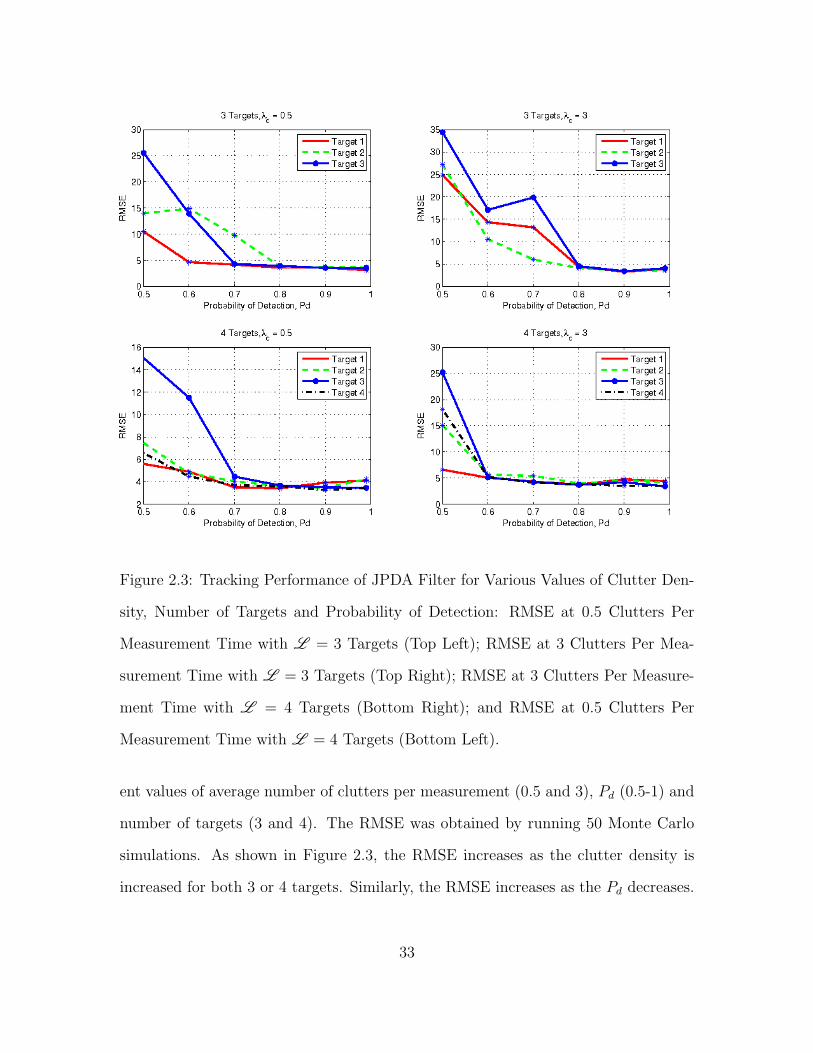
Figure 2.3: Tracking Performance of JPDA Filter for Various Values of Clutter Den-

sity, Number of Targets and Probability of Detection: RMSE at 0.5 Clutters Per

Measurement Time with L = 3 Targets (Top Left); RMSE at 3 Clutters Per Mea-

surement Time with L = 3 Targets (Top Right); RMSE at 3 Clutters Per Measure-

ment Time with L = 4 Targets (Bottom Right); and RMSE at 0.5 Clutters Per

Measurement Time with L = 4 Targets (Bottom Left).

ent values of average number of clutters per measurement (0.5 and 3), Pd (0.5-1) and

number of targets (3 and 4). The RMSE was obtained by running 50 Monte Carlo

simulations. As shown in Figure 2.3, the RMSE increases as the clutter density is

increased for both 3 or 4 targets. Similarly, the RMSE increases as the Pd decreases.

33

This is expected because, when the probability of detection is low, the JPDA filter

can use a fewer number of correct measurements for target tracking. The RMSE for

all targets reaches a steady state condition when the Pd is greater than 0.8. Thus, at

higher Pd values, the JPDA is able to track multiple targets without being drastically

influenced by the presence of multiple targets. However, the tracking performance

begins to degrade when the probability of detection decreases.

2.5 Sequential Monte Carlo Based Joint Probabilistic Data Association

The JPDA discussed in Section 2.4.2 assumed linear and Gaussian state space

models. If the model is nonlinear, then the JPDA filter equations derived using the

KF can be extended to support nonlinear models by using the EKF. However, if

the state space model is not Gaussian, then, the EKF based JPDA filter’s tracking

performance will not be satisfactory. A particle filter (PF) based JPDA technique to

track multiple targets in clutter environment was considered in [31, 32]. Since then,

different PF based techniques [33, 34, 96] have been developed to track multiple

targets in clutter environments for nonlinear and non-Gaussian state space models.

For example, a PF based technique was used in [34] by combining PFs with the

multiple hypothesis tracking method. The computational cost involved with this

method is very expensive. To reduce the computational cost, the authors proposed

to use KF or EKF to track the actual target states and PF to track different target

hypothesis. The target states and the track hypothesis distribution estimate were

then combined using the Rao-Blackwellization technique [97].

2.5.1 Monte Carlo Based JPDA Filter

A generalized Monte Carlo based JPDA (MCJPDA) framework for multiple tar-

get and multiple sensor tracking with data association was presented in [33], with

34

two possible extensions to reduce computational complexity. This MCPJDA method

closely follows the KF based JPDA filter as it uses the same hypothesis probability

calculation method. The main difference is in the estimation of the posterior PDF for

each target. The JPDA filter tries to collapse the posterior PDF into a single Gaus-

sian distribution, whereas, in the MCJPDA filter, the posterior PDF is approximated

by particles. Hence, if the importance distribution is selected appropriately, then the

MCJPDA can approximate any multi-modal distribution without any significant loss

of information.

2.5.2 Data Association and Sequential Monte Carlo

All the assumptions made for JPDA is valid for MCJPDA except for the Gaus-

sian assumptions. The prediction equation for each target in the optimal Bayesian

framework is given by

p(xk,ℓ|zk−1) =

∫p(xk,ℓ|xk−1,ℓ)p(xk−1,ℓ|zk−1)dxk−1,ℓ (2.11)

where zk−1 is the set of all measurement vectors at time step k− 1. As the MCJPDA

is assumed to be a zero scan algorithm, we substitute zk (only the current measure-

ment) for all Zk. Due to measurement origin uncertainty, the update step cannot

be performed independently for each target. In order to solve this data association

problem, the JPDA concept is used to assign measurement-to-target probabilities

such that all measurements are used to update the ℓth target state. Specifically,

the measurement-to-target probabilities are used as weights to obtain the weighted

likelihood function for the ℓth target. The weighted likelihood function is given by

p(zk|xk,ℓ) = β0k,ℓ +

Nk,m∑i=1

βik,ℓp(z

ik|xk,ℓ) (2.12)

where zik is the ith measurement vector at time k, and βik,ℓ is the probability that the

ith measurement is associated with the ℓth target. Based on the modified definition

35

of the likelihood function, the update equation for the optimal Bayesian solution is

given by

p(xk,ℓ|zk) ∝ p(zk|xk,ℓ)p(xk,ℓ|zk−1). (2.13)

The PDF of the predicted measurement can be calculated as

p(zk|zk−1) =

∫p(zk|xk,ℓ)p(xk,ℓ|zk−1)dxk,ℓ. (2.14)

The calculation of the hypothesis probability is exactly the same as for the JPDA.

The recursive Equations (2.11), (2.12) and (2.13) provide a theoretical framework for

tracking multiple targets with measurement origin uncertainty.

2.5.3 Particle Filter Implementation of MCJPDA

In most cases, it is very difficult to derive a closed form solution for a given

dynamic state and measurement model. Hence, we have to resort to particle filters

to approximate the posterior PDF of the target states. For the ℓth target, if we

assume that the approximate posterior PDF is available and it is parameterized as

x(n)k−1,ℓ, w

(n)k−1,ℓNn=1, where N is the number of particles, then the particle filter steps

are given as follows.

• At time step k, generate new samples that are distributed according to the

importance density qℓ(xk,ℓ|x(n)k−1,ℓ, zk),

x(n)k,ℓ ≈ qℓ(xk,ℓ|x(n)

k−1,ℓ, zk)

• Compute the particle filter approximation of the predicted measurement likeli-

hood as

p(zk|zk−1) ≈N∑

n=1

α(n)k,ℓ p(zk|x

(n)k,ℓ )

36

where the predictive weights α(n)k,ℓ are calculated by applying Monte Carlo inte-

gration on Equation (2.14),

α(n)k,ℓ ≈ w

(n)k−1,ℓ

p(x(n)k,ℓ |x

(n)k−1,ℓ)

qℓ(x(n)k,ℓ |x

(n)k−1,ℓ, zk)

,N∑

n=1

α(n)k,ℓ = 1

• Enumerate all possible hypothesis and compute their corresponding probabili-

ties.

• Calculate the measurement-to-target data association probability using the pre-

dicted measurement likelihood and the hypothesis probability.

• Compute the target likelihood PDF in Equation (2.13) based on the computed

data association probability.

• Compute the particle weights for approximating the posterior PDF,

w(n)k,ℓ ≈ w

(n)k−1,ℓ

p(zk|x(n)k,ℓ )p(x

(n)k,ℓ |x

(n)k−1,ℓ)

qℓ(x(n)k,ℓ |x

(n)k−1,ℓ, zk)

• Normalize the weights and resample the particles to avoid sample degeneration.

2.5.4 MCJPDA Using SIR particle filter

Using the aforementioned PF implementation, to generate the particles requires

the importance density and the tracking performance is highly dependent on the

choice of importance density. One simple choice is to use the state transition distri-

bution as the importance density [31],

qℓ(x(n)k,ℓ |x

(n)k−1,ℓ, zk) ≈ p(x

(n)k,ℓ |x

(n)k−1,ℓ).

If the state transition distribution is used, then the measurement likelihood becomes

p(zk|zk−1) ≈1

N

N∑n=1

p(zk|x(n)k,ℓ )

37

and the particle filter weights depend only on the measurement likelihood,

w(n)k,ℓ ≈ w

(n)k−1,ℓp(zk|x

(n)k,ℓ ).

We have implemented the MCJPDA filter using the SIR particle filter in Mat-

lab for tracking multiple targets in the 2-D plane. Unlike previous examples, we

used nonlinear measurement functions to track multiple targets. We used the same

process model as before with the matrix F for all targets as in Equation (2.6). The

measurement vector consists of range rk,ℓ and range-rate rk,ℓ. The nonlinear relation

between the measurements and target states are given by

rk,ℓ =√(xk,ℓ − xo)2 + (yk,ℓ − yo)2 (2.15)

rk,ℓ =xk,ℓ(xk,ℓ − xo) + yk,ℓ(yk,ℓ − yo)√

(xk,ℓ − xo)2 + (yk,ℓ − yo)2(2.16)

where (xo, yo) is the stationary sensor location coordinates. In our simulations, we

assumed Gaussian noise for both the measurement noise and the modeling error

process. We used four targets, whose initial target states are same as the ones used

in the JPDA illustration in Figure 2.2. The process noise parameter q was set to

10−6 and the measurement noise variance for the measurement vector was set at 25

for range and 1 for range-rate measurements. The average number of clutters per

measurement was set at 2, (clutter spatial density λ = 0.002924). The probability

of target detection Pd was set at 0.9 and 300 particle were used to approximate the

posterior PDF. Figure 2.4 shows the original clutter measurement distribution at

all times and also the target associated measurement distribution. From the figure,

it is not possible to visually separate the clutter associated measurements from the

target associated measurements. Figure 2.4 also shows the true and estimated target

position for all four targets and the MCJPDA filter is able to accurately estimate the

38

state vectors. The estimated trajectory deviates from the true trajectory when the

targets came close to each other. However, the MCJPDA filter was able converge

back to the true trajectory after the targets had moved away from each other.

Figure 2.4: MCJPDA Filter Performance: True and Estimated Trajectories for Four

Targets (Top Left); Target and Clutter Associated Measurements (Top Right, Green

and Black Stars Represent Target and Clutter Associated Range Measurements, re-

spectively, and Red and Cyan Dots Represent Target and Clutter Associated Range-

Rate Measurements, respectively); Velocity in the y-direction (Bottom Right); and

Velocity in the x-direction (Bottom Left).

39

Chapter 3

SINGLE TARGET SEQUENTIAL MONTE CARLO TRACK-BEFORE-DETECT

FILTERING

3.1 Tracking Under Low Signal-to-Noise Ratio Conditions

Under low signal-to-noise ratio (SNR) conditions, it is possible to miss the de-

tection of target associated measurements. In conventional radar systems, tracking

low SNR moving targets using constant false alarm rate (CFAR) detectors [45, 46]

can result in poor performance as thresholding can result in a loss of information.

The probability of detection is low for targets with small radar cross section [45, 47],

since, as the SNR decreases, the CFAR detection threshold needs to be increased;

this requires additional measurements, resulting in increased number of false alarms.

The track-before-detect filter (TBDF) is a method proposed to improve track-

ing under low SNR conditions. TBDF algorithms based on the Hough transform,

dynamic programming or maximum likelihood are generally computationally inten-

sive [17]. However, with recent advancements in sequential Monte Carlo techniques,

TBDF algorithms implemented using a particle filter (PF) are now computationally

feasible [51, 52]. The PF based TBDF incorporates unthresholded data and a binary

target existence variable into the target state estimation process. A recursive TBDF

algorithm for a single target was proposed in [55] that uses PF based interacting

multiple model (IMM) concept for a jump Markov nonlinear model [98]. For a single

target, the modes correspond to a target entering the field of view (FOV) and to a

target leaving the FOV. Following the IMM method, the target state estimates from

both modes are integrated to derive the final state estimates.

40

3.2 Sequential Monte Carlo Track-before-detect Filtering

The PF based TBDF (PF-TBDF) proposed in [51] can work using a single scan

of data like the PDA filter families, and it also supports nonlinear and non-Gaussian

state space models.

3.2.1 State Space Model

We assume that we want to track a target moving in a 2-D plane with an unknown

state vector xk at time step k. As in Chapter 2, we consider the state model given by

xk = Fxk−1 + vk (3.1)

where F is the state transition matrix, assuming constant velocity motion and vk

is a modeling error random process with covariance matrix Q. A target can be

present or absent in the measurement space. This is modeled as a random process by

introducing a random variable Ek which is modeled as a two state first order Markov

chain. Specifically, Ek ∈ 0, 1, where Ek = 1 represents the target existence in the

FOV and Ek = 0 represents the target absence in the FOV. We consider two state

transitional probabilities: the probability PB of a target entering the FOV and the

probability PD of a target leaving the FOV. These probabilities are assumed known

and are defined as PB , Pr(Ek = 1|Ek−1 = 0), PD , Pr(Ek = 0|Ek−1 = 1). Once

a target is detected, the probability that the target remains in the FOV is (1− PD).

Similarly, once a target is detected to leave the FOV, the probability that target

remains outside the FOV is given by (1− PB). The corresponding transition matrix

for the Markov process is

Ω =

1− PB PB

PD 1− PD

. (3.2)

41

The initial target existence probability Pr(e0 = 1) is also assumed to be known, where

ek is the event that represents the existence of a target.

We assume that each unthresholded measurement z(a,b)k , with center coordinate in

the 2-D plane given by (a, b), is related to the target state vector according to

z(a,b)k =

h(a,b)k (xk) + w

(a,b)k , for Ek = 1

w(a,b)k , for Ek = 0

(3.3)

where h(a,b)k (xk) is a possibly nonlinear function of xk and the measurement noise w

(a,b)k

is assumed to be independent and Gaussian distributed with variance r. The mea-

surement vector zk consists of multiple unthresholded measurements, as in Equation

(3.3), and

Zk = z0, z1, . . . , zk

where Zk is the set of all measurement vectors up to time step k.

3.2.2 Bayesian Solution to Track-before-detect Filtering

Given the state and measurement models and the posterior probability density

function (PDF) at time step k − 1, p(xk−1, Ek−1|Zk−1), the task of PF-TBDF is to

estimate the posterior PDF at time step k, p(xk, Ek|Zk). This is a multiple-model

problem in which the posterior PDF is dependent on the target existence condition

or mode. For the single target case, there are two modes: target is present and target

is absent. The posterior PDF needs to be estimated only when the target is present

since the posterior PDF is undefined when the target is absent. Using the generic

Bayesian solution for multiple switching dynamic models [17], the predicted PDF for

the PF-TBDF is given by

42

p(xk, Ek = 1|Zk−1) = PB

∫pb(xk) p(xk−1, Ek−1 = 0|Zk−1) dxk−1 +

(1− PD)

∫p(xk|xk−1, Ek−1 = 1, Ek = 1) p(xk−1, Ek−1 = 1|Zk−1) dxk−1 (3.4)

where pb(xk) is an a priori known target distribution based on the assumption that

the target is detected at time step k, and p(xk|xk−1, Ek−1 = 1, Ek = 1) is defined by

the target state transition model. Given the predicted prior PDF and the likelihood

function p(Zk|xk, Ek = 1), the updated PDF can be written as

p(xk, Ek = 1|Zk) =p(Zk|xk, Ek = 1) p(xk, Ek = 1|Zk−1)

p(Zk|Zk−1).

Since, the measurement noise is assumed to be independent between unthresholded

measurements, the joint likelihood function can be written as

p(Zk|xk) =

∏a

∏b

N (z(a,b)k ;h

(a,b)k (xk), r), for Ek = 1

∏a

∏b

N (z(a,b)k ; 0, r), for Ek = 0

(3.5)

where N (z(a,b)k ;h

(a,b)k (xk), r) implies that z

(a,b)k is a Gaussian random variable with

mean h(a,b)k (xk) and variance r.

3.2.3 Particle Filter Implementation of Track-before-detect Filtering

The PF implementation of the aforementioned Bayesian recursive equations was

originally performed in [51] by appending the state vector with the target existence

variable Ek to form yk = [xTk Ek]

T. The posterior PDF of the new state vector yk

is approximated using N particles y(n)k and their corresponding weights w

(n)k , n =

1, . . . , N ; the resulting PF implementation steps are listed next.

• A set of particles for the target existence variable E(n)k are generated using the

past state E(n)k−1 and the state transition matrix Ω.

43

• The target states are predicted based on the target existence condition for each

particle. Based on the current and past state of the target existence variable,

there are two possible modes:

– Mode 1: the target enters the FOV (Ek−1 = 0 and Ek = 1):

The target state particles are uniformly drawn at time step k based on

some a priori information on the minimum and maximum possible values

on the target state.

– Mode 2: the target remains in the FOV (Ek−1 = 1 and Ek = 1):

The state transition model in Equation (3.1) is used to update the target

state particles.

• The particle weights are computed by modifying the likelihood function in Equa-

tion (3.5) as

p(Zk|xk) ∝

∏a

∏b

N (z(a,b)k ;h

(a,b)k , r)∏

a

∏b

N (z(a,b)k ; 0, r)

, for Ek = 1

1, for Ek = 0

∝

∏a

∏b

l(z(a,b)k |xk), for Ek = 1

1, for Ek = 0

(3.6)

where l(z(a,b)k |xk) is the measurement-dependent likelihood ratio.

• The computed weights are normalized and the particles are resampled.

• From the approximated posterior PDF of the appended state vector yk, the

44

target existence probability Pr(ek) is obtained as

Pr(ek) =1

N

N∑n=1

E(n)k .

3.3 Efficient Particle Filter Based Track-before-detect Filtering

3.3.1 Algorithm Description

In the previous section, a PF based TBDF method was described in which the

target existence variable is also included in the state vector. An efficient PF based

method was proposed in [53] that does not include the target existence variable in

the state vector. An analytical expression was also derived to estimate the target

existence probability. Moreover, instead of using a single set of particles, the efficient

PF-TBDF represents each mode (a target entering the FOV and a target remaining

in the FOV) by a set of particles. This efficient approach integrates the PF imple-

mentation algorithm proposed for the IMM algorithm in [98] for a nonlinear jump

Markov system. The two particle sets scheme enables one to efficiently assign dif-

ferent number of particles for the two modes, thereby avoiding particle degeneracy

that typically happens during mode transition. Similar to the original PF-TBDF,

this method also estimates the posterior PDF p(xk, Ek = 1|Zk). The posterior PDF

can be written as

p(xk, Ek = 1|Zk) = p(xk|Ek = 1,Zk) Pr(Ek = 1|Zk). (3.7)

In Equation (3.7), the target existence probability Pr(Ek = 1|Zk) is separated from

the target’s state parameters. The target state vector PDF conditioned on target

45

existence can be written as

p(xk|Ek = 1,Zk) =1∑

j=0

p(xk, Ek−1 = j|Ek = 1,Zk)

= p(xk, |Ek−1 = 0, Ek = 1,Zk) Pr(Ek−1 = 0|Ek = 1,Zk)+

p(xk, |Ek−1 = 1, Ek = 1,Zk) Pr(Ek−1 = 1|Ek = 1,Zk).

(3.8)

Thus, the target state vector PDF conditioned on target existence is a weighted

mixture of two density functions. The density function p(xk, |Ek−1 = 0, Ek = 1,Zk)

represents the target state vector PDF conditioned on a target entering the FOV.

The density function p(xk, |Ek−1 = 1, Ek = 1,Zk) represents the target state vector

PDF conditioned on a target remaining in the FOV. Using Bayes rule, the PDF

corresponding to a target entering the FOV can be updated as

p(xk, |Ek−1 = 0, Ek = 1,Zk) = l(zk|xk, Ek = 1) p(xk, |Ek−1 = 0, Ek = 1)

where p(xk, |Ek−1 = 0, Ek = 1) = pb(xk) is the a priori distribution described below

Equation (3.4) and l(zk|xk, Ek = 1) is the likelihood function in Equation (3.6).

Similarly, the PDF corresponding to a target remaining in the FOV can be updated

as

p(xk, |Ek−1 = 1, Ek = 1,Zk) = l(zk|xk, Ek = 1) p(xk, |Ek−1 = 1, Ek = 1,Zk−1).

The predicted density can be written as a function of the transition density and the

posterior target state distribution at time step k − 1,

p(xk|Ek−1 = 1, Ek = 1,Zk−1) =

∫p(xk|xk−1, Ek−1 = 1, Ek = 1)

p(xk−1, |Ek−1 = 1,Zk−1) dxk−1.

Closed form expressions for the weights Pr(Ek−1 = 0|Ek = 1,Zk) and Pr(Ek−1 =

1|Ek = 1,Zk) in Equation (3.8) are derived in [53].

46

3.3.2 Implementation of the Efficient PF-TBDF

The implementation of the efficient PF-TBDF using a separate particle set for each

mode is described next, following [53]. The posterior PDFs, p(xk, |Ek−1 = 1, Ek =

1,Zk) and p(xk, |Ek−1 = 0, Ek = 1,Zk) are approximated using the particle and

weight sets x(n1)k−1 and w

(n1)k−1 , n1 = 1, . . . , N1 and x

(n2)k−1 and w

(n2)k−1 , n2 = 1, . . . , N2 where

N1 and N2 are the respective number of particles for each set. Given p(xk−1, |Ek−2 =

1, Ek−1 = 1,Zk−1) and the target existence probability Pr(ek−1) at time step k − 1,

the PF steps are listed next.

• At time step k, N2 new particles are generated that are distributed according

to the proposal density

x(n2)k ≈ q(xk|Ek−1 = 0, Ek = 1,Zk).

n2 = 1, 2, . . . , N2 using the steps in Section 3.2.3.

• The corresponding weights are obtained using

w(n2)k =

l(zk|x(n2)k , Ek = 1) q(x

(n2)k |Ek−1 = 0, Ek = 1,Zk)

N2 q(x(n2)k |Ek−1 = 0, Ek = 1,Zk)

.

• The particle weights are normalized

w(n2)k =

w(n2)k∑N2

n2=1 w(n2)k

.

• N1 new particles are generated that are distributed according to the proposal

density

x(n1)k ≈ q(xk|Ek−1 = 1, Ek = 1,Zk)

n1 = 1, 2, . . . , N1 using the target dynamic model in Equation (3.1).

47

• The particle weights are calculated using

w(n1)k =

l(zk|x(n1)k , Ek = 1)

N1

.

• The particle weights are normalized

w(n1)k =

w(n1)k∑N1

n1=1 w(n1)k

.

• The mixing probabilities are calculated as

PrU(Ek−1 = 1|Ek = 1,Zk) = [1− PD] Pr(ek−1)

N1∑n1=1

w(n1)k ,

PrU(Ek−1 = 0|Ek = 1,Zk) = PB [1− Pr(ek−1)]

N2∑n2=1

w(n2)k .

where Pr(ek−1) is the target existence probability at the previous time step,

and PB and PD are the a priori probabilities of a target entering or leaving the

FOV, respectively.

• The mixing probabilities are normalized

Pr(Ek−1 = 0|Ek = 1,Zk) =PrU(Ek−1 = 0|Ek = 1,Zk)

PrU(Ek−1 = 0|Ek = 1,Zk) + PrU(Ek−1 = 1|Ek = 1,Zk),

Pr(Ek−1 = 1|Ek = 1,Zk) =PrU(Ek−1 = 1|Ek = 1,Zk)

PrU(Ek−1 = 0|Ek = 1,Zk) + PrU(Ek−1 = 1|Ek = 1,Zk).

• The probability of target existence is calculated using

Pr(ek) =

[1 +

(1− Pb) (1− Pr(ek−1)) + PD Pr(ek−1)

PrU(Ek−1 = 0|Ek = 1,Zk) + PrU(Ek−1 = 1|Ek = 1,Zk)

]−1

.

• The particle weights are scaled by the mixing probabilities as

w(n1)k = Pr(Ek−1 = 1|Ek = 1,Zk)w

(n1)k ,

w(n2)k = Pr(Ek−1 = 0|Ek = 1,Zk)w

(n2)k .

The two set of particles are then combined to generate N2 + N1 particles.

48

• The particles are resampled and the number of particles are reduced from (N2

+ N1) to N1 to represent the posterior PDF of the target remaining in the FOV.

3.4 Target Tracking Example Using Image Measurements

3.4.1 Image Measurement Model

We consider tracking moving targets using image measurements from video cam-

eras. Each measurement is considered to be a sequence of 2-D image frames with

finite resolution, and each pixel in a frame is characterized by its grey-scale level.

Each 2-D measurement frame is assumed to consists of (Nx ×Ny) pixels with a pixel

resolution (x×y). The center of the pixel (a, b) is at the position (ax× by). If

a target is not present in a frame, the measurement contains only noise for all pixels.

If a target is present in a frame, then the pixels in the vicinity of the target’s current

position contain signal plus noise. A point target and a sensor point spread function

approximated by a 2-D Gaussian function is assumed in this measurement model. If

a target is present in a measurement frame, it is characterized by its x and y coordi-

nate position and its corresponding grey-scale level in that position. The grey-scale

level is denoted as Ik. In addition to the target position and intensity, the component

velocities also constitute the state vector. The targets state vector is then given by

xk = [xk, xk, yk, yk, Ik]T.

49

Assuming constant velocity target motion, the elements of the (5×5) state transition

matrix F is given by

F =

1 ∆T 0 0 0

0 1 0 0 0

0 0 1 ∆T 0

0 0 0 1 0

0 0 0 0 1

where ∆T is the time step interval and we assumed additive noise model for target

intensity. The measurements from all pixels in Equation (3.3) are concatenated to

generate the measurement vector

zk =[z(1,1)k z

(1,2)k . . . z

(1,Nx)k z

(2,1)k z

(2,2)k . . . z

(2,Ny)k . . . z

(Nx,1)k . . . z

(Nx,Ny)k

].

The likelihood function l(z(a,b)k |xk) in Equation (3.6) can be simplified as

l(z(a,b)k |xk) , exp

− h

(a,b)k (xk)(h

(a,b)k (xk)− 2z

(a,b)k )

2r

, (3.9)

where h(a,b)k (xk) is the intensity contribution of a target present at the position (xk, yk)

to the pixel (a, b). The imaging sensor measurement corresponding to a target is

modeled using a Gaussian spread function with a point target assumption. The

blurring introduced by the sensor is modeled by adjusting the spread factor σ, of the

Gaussian spread function. For a target present at the position (xk, yk), this nonlinear

spread function h(a,b)k (xk) in the measurement model in Equation (3.3) can be modeled

as

h(a,b)k (xk) = xyIk

2πσ2 exp− (ax−xk)

2+(by−yk)2

2σ2

. (3.10)

3.4.2 Simulations

We have implemented the two PF-TBDF algorithms in Matlab for tracking a

single target in a 2-D plane under low SNR conditions, following the example used in

50

[17]. The covariance matrix Q for the noise vk in Equation (3.1) is given by

Q =

q1∆T 4

4

q1∆T 3

20 0 0

q1∆T 3

2q1∆T 2 0 0 0

0 0q1∆T 4

4

q1∆T 3

20

0 0q1∆T 3

2q1∆T 2 0

0 0 0 0 q2∆T

where q1 and q2 are the process noise parameters for the target motion and intensity,

Frame :2

10 20

5

10

15

20Frame :7

10 20

5

10

15

20Frame :12

10 20

5

10

15

20

Frame :17

10 20

5

10

15

20Frame :22

10 20

5

10

15

20Frame :27

10 20

5

10

15

20

Figure 3.1: Measurement Frame at Different Time Steps at 20 dB Peak SNR. In all

the Plots, the x and y Axes Correspond to the x and y Coordinates in the FOV,

respectively.

respectively. Similar to the example in [17], 30 frames of measurements were generated

with the following parameters, x = 1, y = 1, Nx = 20, Ny = 20, ∆T = 1 s; the

blurring parameter σ is set at 0.7. The algorithm performance is evaluated under

different peak SNR conditions. The measurements were generated such that a target

51

Frame :2

10 20

5

10

15

20Frame :7

10 20

5

10

15

20Frame :12

10 20

5

10

15

20

Frame :17

10 20

5

10

15

20Frame :22

10 20

5

10

15

20Frame :27

10 20

5

10

15

20

Figure 3.2: Measurement Frame at Different Time Steps at 6 dB Peak SNR.

enters the FOV at time step 7 and leaves the FOV at time step 23. The initial target

position and velocity are set at (4.2,7.2) m, and (0.45 0.25) m/s respectively. Figure

3.1 shows the measurement frame at different time steps and 20 dB peak SNR. Since

the peak SNR is high, the target position can be observed simply by the distinct

pixels. Figure 3.2 shows the measurement frame at 6 dB peak SNR. In this case, it

is not possible to detect the existence of the target by visual inspection. We thus

aim to demonstrate the performance of the PF-TBDF under this low SNR condition.

The noise parameters are set at q1 = 0.001, q2 = 0.01 and r = 1. The state transition

probabilities are assumed to be PB = 0.05, PD = 0.05, Pr(e0) = 0.05. The parameters

used in generating the particles when a target enters the FOV are νmax = 0.5 and

νmin = 0.2. The target intensity range is set to Imin = 10, Imax = 30; this range

reflects the expected 0 to 20 dB peak SNR. The number of particles are set to 15,000

particles for both N1 and N2.

Figure 3.3 shows the target existence probability at 6 dB peak SNR (I0 = 6.14),

52

5 10 15 20 25 300

0.1

0.2

0.3

0.4

0.5

0.6

0.7

0.8

0.9

1

Time Step

Pro

babi

lity

of ta

rget

exi

sten

ce

Figure 3.3: Target Existence Probability at 6 dB Peak SNR (Red Stars Represent

the Time Steps at which the Target Truly Exist).

at different time steps using the efficient PF-TBDF method. As demonstrated in

the figure, the target existence probability is accurately estimated. It takes about

3 frames for the probability to increase after the target enters the FOV, and the

probability decreased quickly after the target left the FOV.

Figure 3.4 shows the particle distribution of the target position variables, and

the histogram of the target intensity. The particle distribution is random before the

appearance of a target. Once the target enters the FOV, the particle distribution

is concentrated around the true target position. Similarly, the particles disperse

after the target leaves the FOV. The same phenomenon is observed with the target

intensity as more particles are concentrated around the true intensity value of 6.14.

Figure 3.5 shows the tracking performance of the efficient PF-TBDF. The top plots

53

5 10 15 20

5101520

Frame :2

0 10 200

100

200Frame :2

5 10 15 20

5101520

Frame :7

0 10 200

200

400Frame :7

5 10 15 20

5101520

Frame :12

0 10 200

100

200Frame :12

5 10 15 20

5101520

Frame :17

0 5 100

100

200Frame :17

5 10 15 20

5101520

Frame :22

0 5 100

100

200Frame :22

5 10 15 20

5101520

Frame :27

0 10 200

100

200Frame :27

Figure 3.4: Particle Distribution for Target Position (Top 6 Plots, where the x and

y Axes Represent the x and y Coordinates in the FOV, respectively); Histogram of

Target Intensity Estimate at Different Frames (Bottom 6 Plots, where the x and y

Axes Represent Intensity and Number of Particles with the Corresponding Intensity

Value, respectively).

of the figure shows the true and estimated target position (shown separately for the

x and y coordinates). From Figure 3.5, the estimates are very close to the true value

after time step 10. The bottom plot shows the true and estimated target trajectory.

As it can be seen, the PF-TBDF was able to closely track the target even under very

low SNR conditions.

The performance of the efficient PF-TBDF is compared with the original PF-

TBDF method using the same number of particles. Figure 3.6 shows the target

54

Figure 3.5: Target Position Estimates, x Coordinate (Top Left); and y Coordinate

(Top Right). True and Estimated Target Trajectory at 6 dB Peak SNR (Bottom).

existence probability under three different peak SNR conditions (12 dB, 6 dB, 3 dB).

The results were obtained by averaging 25 Monte Carlo simulations. The root mean-

squared error (RMSE) between the estimated and true target position is calculated

to compare the two algorithms and the RMSE is calculated using

RMSE =√

(xtrue − xest)2 + (ytrue − yest)2.

Figure 3.7 shows the position RMSE for both methods and both algorithms appear

to have similar detection performance. However, under lower SNR conditions, the

position error using the efficient PF-TBDF is lower than the original PF-TBDF.

In the simulations, it was also observed that the efficient PF-TBDF provides similar

performance even when the number of particles is reduced. However, with the original

55

5 10 15 20 25 300

0.1

0.2

0.3

0.4

0.5

0.6

0.7

0.8

0.9

1

Time Step

Pro

bability o

f ta

rget pre

sence

Efficient particle filter

Particle filter

(a)

5 10 15 20 25 300

0.1

0.2

0.3

0.4

0.5

0.6

0.7

0.8

0.9

1

Time Step

Pro

bability o

f ta

rget pre

sence


Particle filter

(b)

5 10 15 20 25 300

0.1

0.2

0.3

0.4

0.5

0.6

0.7

0.8

0.9

1

Time Step

Pro

bability o

f ta

rget pre

sence


Particle filter

(c)

Figure 3.6: Target Existence Probability for the Original PF-TBDF and the Efficient

PF-TBDF Methods (a) SNR = 12 dB; (b) SNR = 6 dB; and (c) SNR = 3 dB.

PF-TBDF, the performance deteriorates as the number of particles is reduced. In

the original PF-TBDF method, the number of particles used for detecting a target

entering the FOV and for tracking a target remaining in the FOV is unevenly split

between the two target transition modes. This results in inaccurate detection of a

target entering the FOV or inaccurate state estimation of a target remaining in the

FOV. With the efficient PF-TBDF, a fixed number of particles is assigned for both

modes, thus reducing the inaccuracy under each mode.

56

0 5 10 15 20 25 30 0

0.1

0.2

0.3

0.4

0.5

0.6

0.7

0.8

0.9

1

Frame Number

Positio

n E

rror

(RM

SE

)

Efficient Particle Filter

Particle filter

(a)

0 5 10 15 20 25 300

0.5

1

1.5

2

2.5

3

3.5

4

Time Step

Positio

n E

rror

(RM

SE

)

Particle Filter

Efficient Particle filter

(b)

0 5 10 15 20 25 300

1

2

3

4

5

6

Time Step

Positio

n E

rror

(RM

SE

)

Particle Filter

Efficient Particle filter

(c)

Figure 3.7: Position RMSE for the Original PF-TBDF and the Efficient PF-TBDF

Methods (a) SNR = 12 dB; (b) SNR = 6 dB; and (c) SNR = 3 dB.

3.5 Target Tracking Example Using Radar Measurements

3.5.1 Radar Measurement Model

In a general radar system, the sensor measurements are in the form of range

and range-resolution bins, obtained by correlating the received data with the time-

frequency shifted versions of the transmitted baseband signal [45]. The transmitter of

57

a pulse Doppler radar system sends a series ofNp pulses with a pulse repetition interval

time TPRI. Each transmitted pulse s[n] consists of Ns samples and has sampling

frequency fs. The radar receiver receives signals that are reflected by targets and

interfering objects. The signals received over a period of Np pulses is referred to as a

dwell measurement. The range is estimated by keeping track of the round trip delay

for the reflected pulse. The target range rk and the delay τk at the kth transmission

are related as

rk =c τk2

where rk is the range in meters at time step k, c is the velocity of propagation and

τk is the corresponding round trip delay in seconds. If a target is moving, then the

reflected signal undergoes frequency scaling due to the Doppler effect. Under the

narrowband assumption, this frequency scaling is approximated as a frequency shift

that depends on the speed of a moving target. Hence, one can estimate the speed of

a moving target by estimating the Doppler frequency using the measurements from

Np pulses. The Doppler frequency νk and the range-rate rk are related as

νk =2 rkc

fc

where rk is the range-rate in m/s at time step k, and fc is the carrier frequency

in Hz. The received complex baseband signal is first matched-filtered to improve

the SNR. If all transmitted pulses have the same duration and also with the same

pulse repetition interval, the matched filter output is the cross-ambiguity function

between the received and transmitted signal at zero Doppler shift (AF(τ, 0)) [46].

Thus, each sample corresponds to the time lag index which in-turn corresponds to a

particular target range bin. The slow-time samples are then generated by sampling

the matched filtered output every NPRI= fsTPRI samples [45]. The target’s range-rate

is estimated by first estimating the Doppler frequency of the received signal using

58

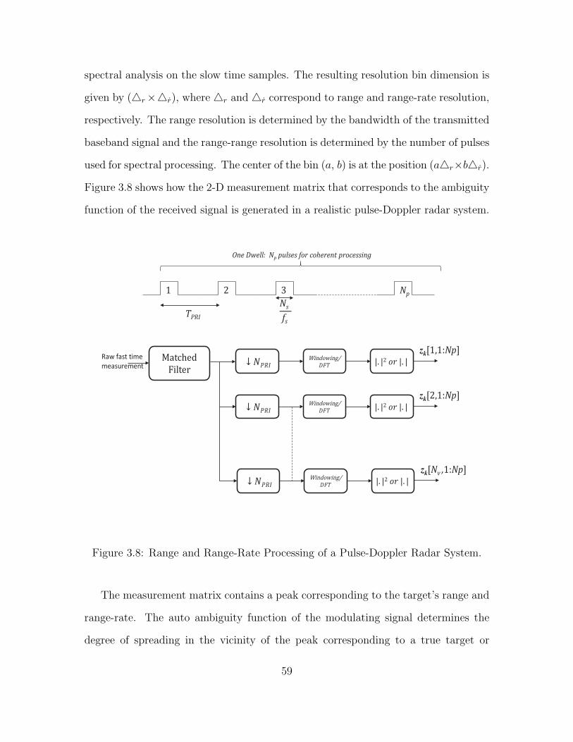
spectral analysis on the slow time samples. The resulting resolution bin dimension is

given by (r×r), where r and r correspond to range and range-rate resolution,

respectively. The range resolution is determined by the bandwidth of the transmitted

baseband signal and the range-range resolution is determined by the number of pulses

used for spectral processing. The center of the bin (a, b) is at the position (ar×br).

Figure 3.8 shows how the 2-D measurement matrix that corresponds to the ambiguity

function of the received signal is generated in a realistic pulse-Doppler radar system.

1 2 3 Np

TPRI

One Dwell: Np pulses for coherent processing

Matched

Filter

Windowing/

|. |2 |. |

zk[1,1:Np]

Windowing/

|. |2 |. |

zk[2,1:Np]

Windowing/

|. |2 |. |

zk[Nv ,1:Np]

Ns

fs

Raw fast time

measurement

Figure 3.8: Range and Range-Rate Processing of a Pulse-Doppler Radar System.

The measurement matrix contains a peak corresponding to the target’s range and

range-rate. The auto ambiguity function of the modulating signal determines the

degree of spreading in the vicinity of the peak corresponding to a true target or

59

clutter. The function h(a,b)k in the measurement Equation (3.3) is related to the range

and range-rate of a particular target as

h(a,b)k (xk) =

∣∣∣∣Ik sin(πNp(νb − νk)TPRI)

sin(π(νb − νk)TPRI)

Ns−1∑n=0

s[na − n− nk]e−j2π(νb−νk)nTPRI

∣∣∣∣ (3.11)

where na is the lag index corresponding to a particular range and νb is the Doppler

frequency corresponding to a particular range-rate in bin (a, b), the relation between

them is given by

na = round

2 ar

cfs

, νb =

2 br

cfc

nk and νk are the lag index and the Doppler frequency corresponding to a target

with a certain range and range-rate, respectively at time step k. The range and the

range-rate are in-turn nonlinearly related to the target state vector xk = [xk xk yk yk]T

where (xk, yk) and (xk, yk) are the 2-D coordinates of the target’s position and velocity

respectively and their relations are given in Equations (2.15) and (2.16).

3.5.2 Simulations Using Rayleigh Measurement Noise

In the image measurement example, the additive measurement noise was assumed

to be Gaussian and this is not always a realistic assumption in radar applications. If

the complex raw measurement is assumed to be Gaussian, then the magnitude spec-

trum of the matched filter output is either Rayleigh or Rician distributed depending

on the existence of a target in a range bin. Thus, the likelihood function in Equation

(3.9) is modified for different measurement noise distributions. The likelihood ratio

with the Rayleigh noise assumption is derived as [53],

l(z(a,b)k |xk) , exp

− [h

(a,b)k (xk)]

2

2r

Io

(− h

(a,b)k (xk)z

(a,b)k

2r

)(3.12)

where I0(·) is the zeroth order modified Bessel function of the first kind and r is the

variance of the in-phase and quadrature components of additive complex Gaussian

noise.

60

In addition to range and range-rate measurements, a radar system can also provide

measurements from the azimuthal and elevation look directions to track a moving

target in a 3-D space. For tracking a target in 2-D space, only the azimuthal look

directions measurement is necessary. In our simulations, we have considered 2-D

space by generating measurements from only one azimuthal direction and the target

positions were restricted to be always present in this direction. We have implemented

a simple pulse-Doppler radar system with the parameters shown in Table 3.1. The

measurements from this simulated radar system is used to track a single moving target

in Rayleigh noise.

0 0.5 1 1.5 2 2.5 3

x 104

−1.5

−1

−0.5

0

0.5

1

1.5

2Radar input, Target Range = 5315.0718 m

Range,m0 0.5 1 1.5 2 2.5 3

x 104

0

20

40

60

80

100

120

140|Matched filter output|, Target Range = 5315.0718 m

Range,m

|y[n

]|

01

23

x 104

−50

0

500

0.5

1

1.5

2

Range, m

Measurement (MF−Slow time sampling−DFT)

Range−Rate, m/s 01

23

x 104

−50

0

500

0.5

1

Range, m

Analytical measurements for noise free signal

Range−Rate, m/s

Figure 3.9: Signal Condition at Various Points in the Radar System at 15 dB Peak

SNR: Raw Received Signal (Top Left); Matched Filter Output (Top Right); Noise-

Free Range and Range-Rate Measurement (Bottom Right); and Noisy Range and

Range-Rate Measurement (Bottom Left).

Figure 3.9 shows the complex radar input signal, the matched filter output, noisy

measurement at 15 dB peak SNR and the noise-free measurement. For the chosen

61

Table 3.1: Simulated Pulse-Doppler Radar System Parameters

Radar Parameter Value

Azimuthal Look Direction 45o

Beamwidth 30o

Carrier Frequency 10.0 GHz

Baseband Signal pulse

Range Gate [1500, 30000] m

Maximum Velocity 37.5 m/s (135 km/hr)

Maximum Doppler Shift 2.5 kHz

Pulse Width 10 µs

Pulse Interval, TPRI 200 µs

Duty Cycle 0.05

Number of Pulses, Np 32

Fast Time Sampling, fs 1.6 MHz

Range Resolution 1500 m

Range-Rate Resolution 2.34 m/s

Measurement Sampling Interval 20 s

State Model Constant velocity

Measurement Model Nonlinear with Rayleigh noise

Tracker PF-TBDF

Number of Particles 4,000 + 4,000 = 8,000

62

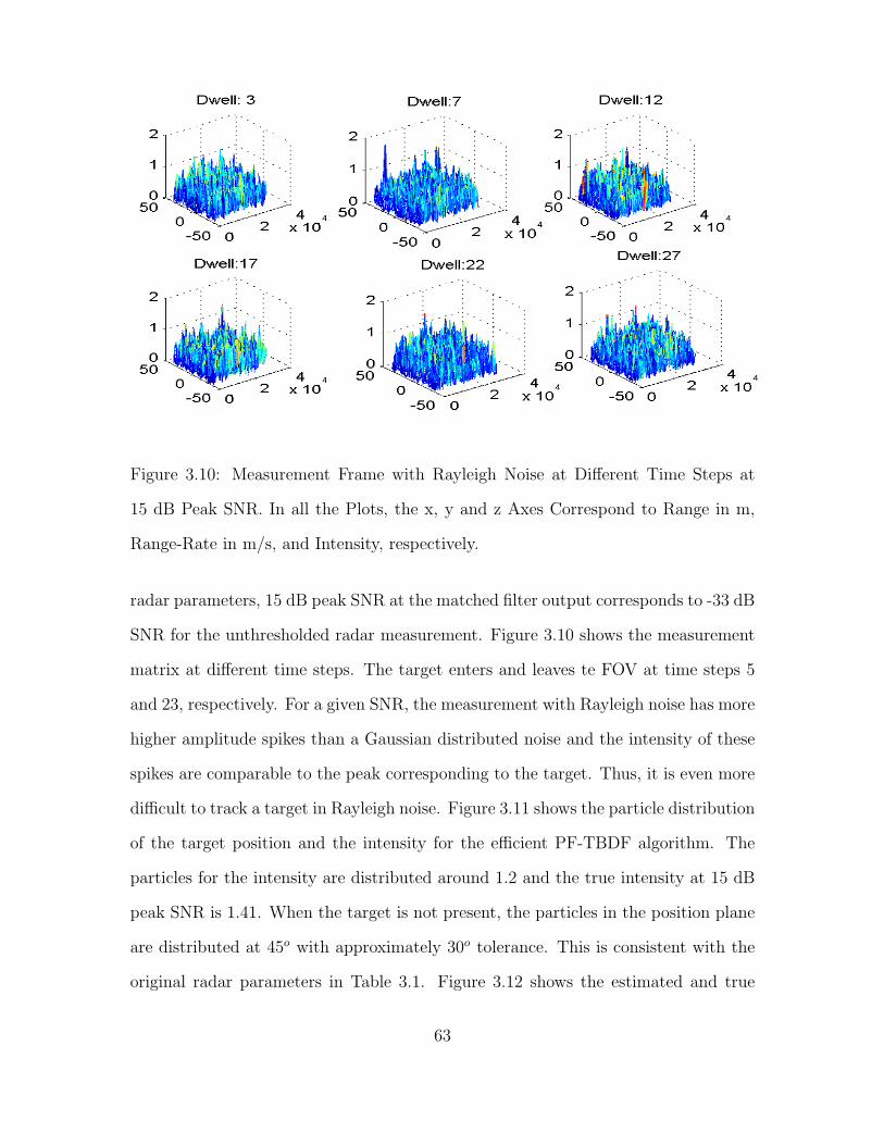
Figure 3.10: Measurement Frame with Rayleigh Noise at Different Time Steps at

15 dB Peak SNR. In all the Plots, the x, y and z Axes Correspond to Range in m,

Range-Rate in m/s, and Intensity, respectively.

radar parameters, 15 dB peak SNR at the matched filter output corresponds to -33 dB

SNR for the unthresholded radar measurement. Figure 3.10 shows the measurement

matrix at different time steps. The target enters and leaves te FOV at time steps 5

and 23, respectively. For a given SNR, the measurement with Rayleigh noise has more

higher amplitude spikes than a Gaussian distributed noise and the intensity of these

spikes are comparable to the peak corresponding to the target. Thus, it is even more

difficult to track a target in Rayleigh noise. Figure 3.11 shows the particle distribution

of the target position and the intensity for the efficient PF-TBDF algorithm. The

particles for the intensity are distributed around 1.2 and the true intensity at 15 dB

peak SNR is 1.41. When the target is not present, the particles in the position plane

are distributed at 45o with approximately 30o tolerance. This is consistent with the

original radar parameters in Table 3.1. Figure 3.12 shows the estimated and true

63

target position and the PF-TBDF method is able to accurately track a target in

Rayleigh noise.

0 1 2

x 104

0

1

2

x 104 Dwell :3

0 1 2 3 40

200

400Dwell :3

0 1 2

x 104

0

1

2

x 104 Dwell :7

0 1 2 30

50

100Dwell :7

0 1 2

x 104

0

1

2

x 104 Dwell :12

0.5 1 1.5 20

10

20Dwell :12

0 1 2

x 104

0

1

2

x 104 Dwell :17

0.5 1 1.5 20

10

20Dwell :17

0 1 2

x 104

0

1

2

x 104 Dwell :22

0 0.5 1 1.5 20

10

20Dwell :22

0 1 2

x 104

0

1

2

x 104 Dwell :27

0 0.5 1 1.5 20

10

20Dwell :27

Figure 3.11: Particle Distribution for Target Position at 15 dB Peak SNR (Top 6

Plots, where the x and y Axes Represent the x and y Coordinates in the FOV, re-

spectively); and Histogram of Target Intensity Estimate at Different Frames (Bottom

6 Plots, where the x and y Axes Represent Intensity and Number of Particles with

the Corresponding Intensity Value, respectively).

64

Figure 3.12: Target Position Estimates, x Coordinate (Top Left); y Coordinate (Top

Right). True and Estimated Target Trajectory at 15 dB Peak SNR (Bottom).

3.5.3 Simulations with Measurements in Clutter

We investigate the PF-TBDF performance for tracking a target in the presence

of clutter. Although the measurement model does not explicitly include clutter, we

can still consider the clutter as a target. If we assume that there is no consistent

trajectory for the clutter, then the PF-TBDF should inherently ignore the clutter as

a consistent moving target thereby rejecting the clutter as noise. The amplitude of

the clutter can be modeled by various distributions [99]. The type of distribution

to use depends greatly on the specific radar application scenario. For example, sea

clutter from a low grazing angle radar is modeled using heavy tailed distributions

65

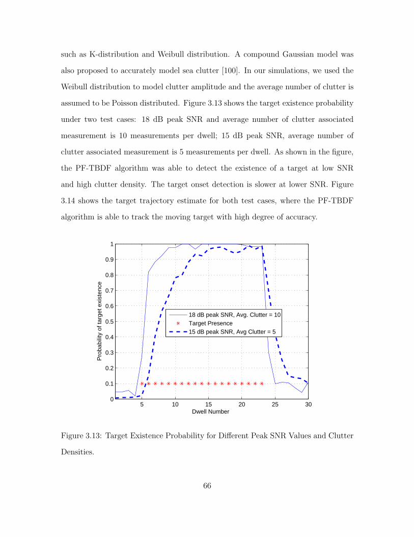
such as K-distribution and Weibull distribution. A compound Gaussian model was

also proposed to accurately model sea clutter [100]. In our simulations, we used the

Weibull distribution to model clutter amplitude and the average number of clutter is

assumed to be Poisson distributed. Figure 3.13 shows the target existence probability

under two test cases: 18 dB peak SNR and average number of clutter associated

measurement is 10 measurements per dwell; 15 dB peak SNR, average number of

clutter associated measurement is 5 measurements per dwell. As shown in the figure,

the PF-TBDF algorithm was able to detect the existence of a target at low SNR

and high clutter density. The target onset detection is slower at lower SNR. Figure

3.14 shows the target trajectory estimate for both test cases, where the PF-TBDF

algorithm is able to track the moving target with high degree of accuracy.

5 10 15 20 25 300

0.1

0.2

0.3

0.4

0.5

0.6

0.7

0.8

0.9

1

Dwell Number

Pro

babi

lity

of ta

rget

exi

sten

ce

18 dB peak SNR, Avg. Clutter = 10Target Presence15 dB peak SNR, Avg Clutter = 5

Figure 3.13: Target Existence Probability for Different Peak SNR Values and Clutter

Densities.

66

0 5 10 15 200

2

4

6

8

10

12

14

16

18

20

x co−ordinate, km

y co

−ord

inat

e, k

m

Target position estimate

xtrue

xest

(a)

0 5 10 15 200

2

4

6

8

10

12

14

16

18

20

x co−ordinate, km

y co

−ord

inat

e, k

m


xtrue

xest

(b)

Figure 3.14: True and Estimated Target Trajectory: (a) SNR = 18 dB, 10 Clutter

Measurements Per Dwell; and (b) SNR = 15 dB, 5 Clutter Measurements Per Dwell.

67

Chapter 4

MULTIPLE TARGET TRACK-BEFORE-DETECT FILTERING

4.1 Tracking Multiple Targets Under Low Signal-to-Noise Ratio Conditions

The track-before-detect filter (TBDF) algorithm discussed in Chapter 3 was ex-

tended to track multiple targets [101], as mentioned in Chapter 1. However, this

method was only shown to work well for a small number of targets. The state vector

dimension in this method does not account for a varying number of targets, and it

does not completely address the uncertainty in the actual number of existing targets.

Recently, an RFS-based approach, the labeled multiple Bernoulli filter has been used

to track multiple targets under low signal-to-noise ratio (SNR) conditions [74].

In this chapter, given a known maximum possible number of targets, we provide

an alternate algorithm that generalizes the recursive TBDF in [53] to track a vary-

ing number of targets in low SNR and high clutter [76, 77] without any need for an

explicit track management step. Since the number of targets that are present in the

field of view (FOV) is not known a priori, we estimate the joint posterior probability

density function (PDF) under all possible target existence combinations [76]. These

joint PDFs are derived under the recursive Bayesian framework, and the state vectors

corresponding to all the targets in the different modes are then appropriately mixed to

derive the overall target state estimates. This is an interacting multiple model (IMM)

algorithm in which the different target motion models in the regular IMM structure

are replaced by all possible target existence combinations or modes. Hence, we refer

to our algorithm as multiple mode multiple target TBDF (MM-MT-TBDF) to differ-

entiate from the regular IMM algorithm [102]. The probability corresponding to each

68

mode is also calculated, and the existence probability of each target is calculated from

this mode probability. We avoid an explicit track management step by estimating an

exhaustive set of multi-target posterior PDFs such that the target-to-track associa-

tion is implicitly achieved through the unique definition of target combinations. The

target states are validated using the estimated target existence probability. We also

propose a particle filter (PF) implementation of the MM-MT-TBDF method that can

also support nonlinear and non-Gaussian models. Although the PHDF approach is

an encompassing framework, it is still not possible to practically estimate the joint

PDF of the multi-target state vector for a time-varying number of targets. Recent

advances in agile radar processing [103] require the posterior PDF of the state vec-

tor to dynamically select waveform parameters. For example, a single target TBDF

based waveform design technique was considered in [104] that uses the posterior PDF

estimate to minimize the tracking error. Using this approach, the set of estimated

joint PDFs at time step k can be used to predict the tracking error at time step k+1

and the waveform parameters at time step k+1 that minimizes the predicted tracking

error can be optimally selected [103].

4.2 Multiple Mode Multiple Target Tracking Model

4.2.1 State Model for Dynamically-varying Number of Targets

We consider the radar problem of tracking a maximum number of L targets. We

define the state vector corresponding to the ℓth target, ℓ=1, . . . ,L at time step k as

xk,ℓ = [xk,ℓ xk,ℓ yk,ℓ yk,ℓ Ik,ℓ]T

where (xk,ℓ, yk,ℓ), (xk,ℓ, yk,ℓ), and Ik,ℓ are the ℓth target’s two-dimensional (2-D)

Cartesian coordinates for position and velocity, and radar cross section (RCS) inten-

sity level, respectively, and T denotes vector transpose. This definition of state vector

69

is appropriate for an air-to-ground or ground-to-ground radar systems in which tar-

gets are localized on the ground. Possible applications may include tracking moving

cars on a rural road or tracking small boats on the sea surface. Note that the state

vector could be easily extended to 3-D space to include target tracking radar sys-

tem applications such as ground-to-air or air-to-air. The multi-target state model we

propose accounts for the fact that not all targets are present at each time step. In

particular, at any time step, targets can enter, leave or remain in the FOV. The total

number of possible target existence combinations or modes is M =2L . This number

includes the case of no targets present, all L targets present, and all possible combi-

nations of L − 1,L − 2, . . . , 1 targets present. Mode i=1 assumes that no targets

are present and mode i=M assumes that all L targets are present. Note that we

assume that the order in which the targets appear in the FOV is not important. We

introduce a binary target presence indicator variable Ciℓ ∈ 0, 1, i=1, . . . ,M , with

1 (or 0) if the ℓth target is present (or is not present) in the ith mode. A simple

example with M =4 modes for L =2 targets is demonstrated in Table 4.1. In our

Table 4.1: Target Presence Indicator Values for L =2 Targets (M =4 Modes).

Mode Target presence indicator values

i C i2 C i

1 Target 2 Target 1

1 0 0 not present not present

2 0 1 not present present

3 1 0 present not present

4 1 1 present present

proposed method, we keep track of all possible target combinations and estimate the

joint posterior PDF of the state vector corresponding to all target combinations. The

70

state vector dimension is determined by the number of possible targets Li in the

ith mode. The target state vector in each mode at time step k is expressed as x[i]k ,

i = 2, . . . ,M to take into consideration the varying number of targets and the result-

ing changes in the multi-target state vector dimension. For example, the multi-target

state vector for the Mth mode is x[M ]k = [xT

k,1 xTk,2 . . . xT

k,L ]T since all L targets are

present in this mode. The state vector for all other modes can be defined from x[M ]k

as x[i]k = PM→ix

[M ]k , where the projection matrix of size (5Li × 5L ) is defined as

PM→i =

[eJ [i](1) . . . . . . eJ [i](Li)

]T⊗ I5 (4.1)

where J [i] is the set (arranged in increasing order) of all targets that are assumed

present in mode i, en is the (L × 1) binary vector whose elements are zero except

the nth element set to one, I5 is the (5× 5) identity matrix, and ⊗ is the Kronecker

product. For example, with M = 4 modes for L = 2 targets, the projection matrix

P4→2 to obtain the state vector for the mode that contains only Target 1 (i = 2 in

Table 4.1) can be written as

P4→2 =

[1 0

]⊗ I5 =

1 0 0 0 0 0 0 0 0 0

0 1 0 0 0 0 0 0 0 0

0 0 1 0 0 0 0 0 0 0

0 0 0 1 0 0 0 0 0 0

0 0 0 0 1 0 0 0 0 0

.

The state vector for mode i = 2 is obtained as

x[2]k = P4→2x

[4]k =

1 0 0 0 0 0 0 0 0 0

0 1 0 0 0 0 0 0 0 0

0 0 1 0 0 0 0 0 0 0

0 0 0 1 0 0 0 0 0 0

0 0 0 0 1 0 0 0 0 0

xk,1

xk,2

.

71

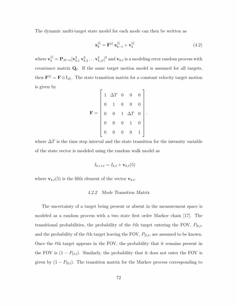
The dynamic multi-target state model for each mode can then be written as

x[i]k = F[i] x

[i]k−1 + v

[i]k (4.2)

where v[i]k = PM→i[v

Tk,1 v

Tk,2 . . .v

Tk,L ]T and vk,ℓ is a modeling error random process with

covariance matrix Qℓ. If the same target motion model is assumed for all targets,

then F[i] = F⊗ ILi. The state transition matrix for a constant velocity target motion

is given by

F =

1 ∆T 0 0 0

0 1 0 0 0

0 0 1 ∆T 0

0 0 0 1 0

0 0 0 0 1

.

where ∆T is the time step interval and the state transition for the intensity variable

of the state vector is modeled using the random walk model as

Ik+1,ℓ = Ik,ℓ + vk,ℓ(5)

where vk,ℓ(5) is the fifth element of the vector vk,ℓ.

4.2.2 Mode Transition Matrix

The uncertainty of a target being present or absent in the measurement space is

modeled as a random process with a two state first order Markov chain [17]. The

transitional probabilities, the probability of the ℓth target entering the FOV, PB,ℓ,

and the probability of the ℓth target leaving the FOV, PD,ℓ, are assumed to be known.

Once the ℓth target appears in the FOV, the probability that it remains present in

the FOV is (1 − PD,ℓ). Similarly, the probability that it does not enter the FOV is

given by (1 − PB,ℓ). The transition matrix for the Markov process corresponding to

72

the ℓth target can then be written as

Tℓ =

1− PB,ℓ PB,ℓ

PD,ℓ 1− PD,ℓ

.

In addition to estimating the joint posterior PDF of each mode, we also estimate the

probability of mode mk at time step k. This variable is modeled as a discrete random

process following an M -state first order Markov chain. Specifically, the probability

that the mode changes from mode j at time k − 1 to mode i at time k is given by

Ωj,i=Pr(mk = i|mk−1= j), i, j=1, . . . ,M . Assuming that the individual target tran-

sitions are independent of each other, we construct the (M×M) transition probability

matrix Ω using the a priori transition matrix of each individual target Tℓ. Specif-

ically, for a given number of targets L , we generalize the mode transition matrix

as

Ω = T1 ⊗T2 . . .⊗TL . (4.3)

Note that the sum of the mode transition probabilities along any row of Ω is unity

and 0 ≤ Ωj,i ≤ 1. The target presence indicator value C iℓ = q, q ∈ 0, 1, i=1, . . . ,M ,

is defined as q=1 (or q=0) if the ℓth target is present (or is not present) in the ith

mode. For the simple example with M =4 modes for L =2 targets in Table 4.1, the

corresponding (4 × 4) mode transition matrix assuming that both targets have the

same transition matrix T1 = T2 and PB1 = PB2 = PB and PD1 = PD2 = PD, is given

by

Ω =

(1− PB)2 PB(1− PB) (1− PB)PB P 2

B

PD(1− PB) (1− PD)(1− PB) PDPB (1− PD)PB

(1− PB)PD PBPD (1− PD)(1− PB) PB(1− PD)

P 2D (1− PD)PD PD(1− PD) (1− PD)

2

(4.4)

73

In practice, it may be difficult to obtain a priori information on transition proba-

bilities of individual targets entering or leaving a scene. Hence, we can assume that

these event probabilities are identical for all targets, i.e., PB,ℓ=PB and PD,ℓ=PD for

ℓ=1, . . . ,L .

4.2.3 Measurement Model Using Image Data

Each measurement frame is assumed to consists of (Nx × Ny) pixels. The pixel

resolution cell dimension is given by (x ×y). The center of the pixel (a, b) is at

the position (ax× by). If no targets are present in a frame, then the measurement

contains only noise for all pixels. If a target is present in a frame, then the pixels

in the vicinity of the target’s current position contain both signal and noise. We

consider point targets and a sensor point spread function approximated by a 2-D

Gaussian density. Unlike the single target TBDF, when there is at least one target, the

measurement function varies depending on the mode at time step k. The measurement

model for multiple targets is given by

z(a,b)k =

Li∑ℓ=0

Ciℓ h

(a,b)k (x

[i]k,ℓ) + w

(a,b)k , for i = 2, . . . ,M

w(a,b)k , for i = 1

, (4.5)

h(a,b)k (x

[i]k,ℓ) =

xyIk,ℓ2πΣ2 exp

− (ax−xk,ℓ)

2+(by−yk,ℓ)2

2Σ2

, (4.6)

where Σ is a known parameter that controls the blurring introduced by the sensor

and x[i]k,ℓ is the ℓth target’s state vector in mode i. The measurement noise w

(a,b)k in

each pixel is assumed to be independent and Gaussian distributed with variance r.

Similar to the single target case, the measurement vector is given by

zk =[z(1,1)k z

(1,2)k . . . z

(1,b)k z

(2,1)k z

(2,2)k . . . z

(2,b)k . . . z

(a,1)k . . . z

(a,b)k

]T74

and

Zk = [zT1 zT2 . . . zTk]T

where Zk is the vector of all the measurements up to time k.

4.2.4 Measurement Model Using Radar Data

As we are using the TBDF for multiple targets, the measurement model uses

unthresholded measurements, similar to the single target case in Chapter 3. We

assume that the measurement frame consists of pre-processed data from a radar

system for different range rk,ℓ, range-rate rk,ℓ and azimuthal angle θk,ℓ bins for the ℓth

target. One example of a measurement frame could be the cross-ambiguity function

between the transmitted and radar received signal. Measurements from independent

multiple sensors are integrated in the problem formulation. The range, range-rate

and azimuthal angle are related to the state vector as

rk,ℓ =√(xk,ℓ − xs)2 + (yk,ℓ − ys)2

rk,ℓ =xk,ℓ(xk,ℓ − xs) + yk,ℓ(yk,ℓ − ys)√

(xk,ℓ − xs)2 + (yk,ℓ − ys)2

θk,ℓ = arctan

(yk,ℓ − ysxk,ℓ − xs

)and the sensor is located at (xs, ys).

Each measurement frame is assumed to consist of (Nr × Nr × Nθ) bins. The

range, range-rate and azimuthal angle bin resolutions are denoted by ∆r,∆r,∆θ,

respectively. The (a, b, c)th cell for a = 1, 2, . . . , Nr, b = 1, 2, . . . , Nr, c = 1, 2, . . . , Nθ,

is then centered around (a∆r×b∆r×c∆θ). The measurements in all the bins simply

consists of noise if no targets are present. If a target is present, then the measurements

in the bins that are in the vicinity of the target’s current position consist of both signal

and noise. We assume a point target model and a sensor point spread function that

75

can be approximated by a 3-D Gaussian function. Based on this assumption, the

measurement equation is given by

z(a,b,c)k =

Li∑ℓ=1

C iℓ h

(a,b,c)k (x

[i]k,ℓ) + v

(a,b,c)k , i = 2 . . .M

v(a,b,c)k , i = 1

(4.7)

where Ciℓ is the target presence indicator value in Equation (4.3) of the ℓth target in

the ith mode, and

h(a,b,c)k (x

[i]k,ℓ)= Ak exp

(−(

a∆r−rk,ℓ2σr

)2

−(

b∆r−rk,ℓ2σr

)2

−(

c∆θ−θk,ℓ2σθ

)2). (4.8)

where Ak =∆r∆r∆θIk,ℓ

(2π)3/2σr,σr,σθis the normalized amplitude, Ik,ℓ is the intensity of the

received signal from the ℓth target and σr, σr, σθ are known parameters that control

the spreading introduced by the radar system. Note that, these parameters can

normally be derived from the ambiguity function of the radar transmitted signal [45].

The independent and identically distributed measurement noise samples v(a,b,c)k in

Equation (4.7) are assumed to be Gaussian with zero-mean and variance νk. The

overall measurement vector is given by

zk,s = [z(1,1,1)k,s . . . z

(1,1,Nθ)k,s . . . z

(1,Nr,Nθ)k,s . . . z

(Nr,Nr,Nθ)k,s ]T

and the sequence zk = [zTk,1 zTk,2 . . . zTk,S]T is the set of all measurements from all

S independent and homogeneous sensors and Zk = [zT1 zT2 . . . zTk]T represents all the

measurements up to time k.

4.3 Multiple Mode Multiple Target Track-before-detect Filtering

4.3.1 Posterior Density for Multiple Mode Multiple Targets

In a multi-target tracking problem with a varying number of targets, the number

of existing targets is not known a priori. Hence, we provide a set of joint distributions

76

of multi-target state vectors conditioned on all possible target existence combinations

and the corresponding probability of different target combinations. In a broader

sense, this is similar to a multiple hypothesis tracking algorithm in which each mode

is equivalent to a hypothesis. Unlike the single target recursive TBDF in [53], we

estimate two different sets of conditional PDFs. The first set of PDFs corresponds

to the posterior joint PDFs conditioned on the mode state at time steps (k − 1) and

k, and the second set of PDFs belongs to the posterior joint PDF conditioned on the

mode state at time step k only. The second set of PDFs are obtained as a weighted

mixture of a subset of the first set of joint PDFs that have the same state vector

dimension. These subset of PDFs are the PDFs that transitioned to a particular

mode from all possible modes. Once we have a set of mode-conditioned PDFs, we

can derive the PDFs of individual target states as a weighted linear combination of

marginalized PDFs that are conditioned on all relevant modes in which the targets

are assumed present. Thus, our approach uses a discrete PDF to characterize all

possible target combinations and the corresponding joint PDFs of the target states

are characterized by continuous distributions. This is similar to the random finite

set approach in which the target states of a random set is modeled by a continuous

distribution and the cardinality of the random set is modeled by a discrete distribution

[37]. Specifically, given the state and measurement models and the posterior PDF

p(x[i]k−1|Zk−1), ∀ i, at time k−1, the MM-MT-TBDF estimates the posterior PDF

p(xk,ℓ|Zk) at time k and the corresponding target existence probability Pr(ek,ℓ|Zk),

where ek,ℓ is the event corresponding to the ℓth target’s presence. We assume that

the initial mode probability, Pr(m0= i|Z0), i=1, . . . ,M , is known a priori. If this

value is not known, then we can assume that no targets are initially present, i.e., we

can assume that Pr(m0= i|Z0)= 0, for i=2, . . . ,M , and Pr(m0=1|Z0)= 1.

The tracking of multiple targets, assuming a varying number of targets, is a mul-

77

tiple mode problem in which the posterior PDF, including the dimension of the state

vector, is dependent on the target mode. As the different modes are mutually exclu-

sive, Pr(mk = i,mk = j|Zk)= 0, ∀ i = j, the posterior PDF can be written as

p(xk,ℓ|Zk) =M∑i=1

Ciℓ p(x

[i]k,l,mk = i |Zk) (4.9)

where x[i]k,l is the state vector corresponding to the ℓth target present in mode i. Here,

even though the superscript [i] and the mode condition eventmk = i seems redundant,

we explicitly denote the state vector as x[i]k,l to emphasize the fact that the dimension

of the state vector in mode i varies with the number of assumed targets in mode i.

The marginal PDF is obtained by marginalizing the joint PDF which can be written

as

p(x[i]k ,mk = i |Zk) = p(x

[i]k |mk = i,Zk) Pr(mk = i |Zk)

for i = 2, . . . , M and Pk,i , Pr(mk = i |Zk) is the posterior mode probability. Note

that we do not include i=1 in this range as we do not need to estimate the posterior

PDF when no targets are present. Using the Bayesian solution for multiple switching

models [17], the target state PDF conditioned on a particular mode can be obtained

as the weighted mixture of M density functions

p(x[i]k |mk = i,Zk

)=

M∑j=1

p(x[i]k |mk−1 = j,mk = i,Zk) Pr(mk−1 = j|mk = i,Zk)

=M∑j=1

pj,i(x[i]k |Zk) Pr(mk−1 = j|mk = i,Zk) (4.10)

for i = 2, . . . ,M . The target state PDF p(x[i]k |mk−1= j,mk = i,Zk) conditioned on

transitioning from mode j at time k−1 to mode i at time k is denoted by pj,i(x[i]k |Zk).

Given the mode state at time step k, the mixing weights Pr(mk−1= j|mk = i,Zk)

provide the probability that the current state is transitioned from mode j at time

78

step k-1. Using Bayes rule, the above mentioned mode conditioned state PDF can be

expanded as

pj,i(x[i]k |Zk) =

p(zk|mk−1 = j,mk = i,x[i]k ) p(x

[i]k |mk−1 = j,mk = i,Zk−1)

p(zk|mk−1 = j,mk = i,Zk−1)

=pj,i(zk|x[i]

k ) pj,i(x[i]k |Zk−1)

pj,i(zk|Zk−1)(4.11)

where we denote p(zk|mk−1 = j,mk = i,x[i]k ), p(x

[i]k |mk−1 = j,mk = i,Zk−1), and

p(zk|mk−1 = j,mk = i,Zk−1) by pj,i(zk|x[i]k ), pj,i(x

[i]k |Zk−1), and pj,i(zk|Zk−1), respec-

tively. If we divide both numerator and denominator by p(zk|mk =0), which assumes

that no targets are present [51], we can express the posterior PDF as a function of

the likelihood ratios,

Lj,i(zk|x[i]k ) =

pj,i(zk|x[i]k )

p(zk|mk = 0),

Lj,i(zk|Zk−1) =pj,i(zk|Zk−1)

p(zk|mk = 0),

as

pj,i

(x[i]k |Zk

)=

Lj,i

(zk|x[i]

k

)pj,i

(x[i]k |Zk−1

)Lj,i(zk|Zk−1)

(4.12)

where the denominator is the normalization term

Lj,i(zk|Zk−1) =

∫Lj,i

(zk|x[i]

k

)pj,i

(x[i]k |Zk−1

)dx

[i]k (4.13)

and Lj,i(zk|x[i]k ) is the joint likelihood function conditioned on the previous and current

modes. Note that, when no targets are present, the likelihood function does not

depend on the target state or the mode condition at previous time step.

79

4.3.2 Likelihood Function for Image Measurements

Since the measurement noise is assumed to be independent between pixels, the

joint likelihood function in Equation (4.11) can be written as

pj,i(zk|x[i]k )=

Nx∏a=1

Ny∏b=1

N (z(a,b)k ; Υ

(a,b)k (x

[i]k ), νk), mk−1 = 1 . . .M, mk = 2 . . .M

Nx∏a=1

Ny∏b=1

N (z(a,b)k ; 0, νk), mk = 1

where N (z(a,b)k ; Υ

(a,b)k (x

[i]k ), νk) implies that z

(a,b)k has a Gaussian distribution with

mean Υ(a,b)k (x

[i]k ) and variance νk, Υ

(a,b)k (x

[i]k )=

∑Lℓ=1 C

iℓ h

(a,b)k (x

[i]k,ℓ) is the cumulative

contribution to pixel (a, b) from all the targets in mode i and h(a,b)k (x

[i]k,ℓ) is defined

in Equation (4.6) in Section 4.2.3. The likelihood ratio in Equation (4.13) can be

written as

Lj,i(zk|x[i]k ) =

Nx∏a=1

Ny∏b=1

N (z(a,b)k ; Υ

(a,b)k (x

[i]k ), νk)

Nx∏a=1

Ny∏b=1

N (z(a,b)k ; 0, νk)

, mk−1 = 1 . . .M, mk = 2 . . .M

1, mk = 1

=

∏

aϵβx(x[i]k )

∏bϵβy(x

[i]k )

l(z(a,b)k |x[i]

k ), mk−1 = 1 . . .M, mk = 2 . . .M

1, mk = 1

(4.14)

where βx(x[i]k ) and βy(x

[i]k ) are the set of pixels in the neighbourhood of the pixels

corresponding to those in which the targets in mode i are present and the likelihood

ratio in Equation (4.14) can be derived as

l(z(a,b)k |x[i]

k ) , exp

− Υ

(a,b)k (x

[i]k )(Υ

(a,b)k (x

[i]k )− 2z

(a,b)k )

2νk

.

80

4.3.3 Likelihood Function for Radar Measurements

Since the measurement noise is assumed independent between bins, the joint like-

lihood function in Equation (4.11), when the measurement consists of range and

range-rate in Equation (4.7), can be written as

pj,i(zk|x[i]k )=

Nr∏a=1

Nr∏b=1

Nθ∏c=1

N (z(a,b,c)k ; Υ

(a,b,c)k (x

[i]k ), νk), mk−1 = 1 . . .M, mk = 2 . . .M

Nr∏a=1

Nr∏b=1

Nθ∏c=1

N (z(a,b,c)k ; 0, νk), mk = 1

where Υ(a,b,c)k (x

[i]k )=

∑Lℓ=1C

iℓ h

(a,b,c)k (x

[i]k,ℓ) is the cumulative contribution to bin (a, b, c)

from all the targets in mode i and h(a,b,c)k (x

[i]k,ℓ) is defined in Equation (4.8) in Section

4.2.4. In order to reduce the computational load, only the bins in the neighbourhood

of existing targets are used. The likelihood function in Equation (4.12) can be written

as

Lj,i(zk|x[i]k ) =

∏

aϵβr(x[i]k )

∏bϵβr(x

[i]k )

∏cϵβθ(x

[i]k )

λ(z(a,b,c)k |x[i]

k ), mk−1 = ∀ M, mk = 2 . . .M

1, mk = 1

(4.15)

where βr(x[i]k ), βr(x

[i]k ) and βθ(x

[i]k ) are the set of all range, range-rate and azimuthal

angle bin numbers, respectively, that are in the neighborhood of the bin numbers

corresponding to those in which the targets in mode i are present and

λ(z(a,b,c)k |x[i]

k ) , exp

− Υ

(a,b,c)k (x

[i]k )(Υ

(a,b,c)k (x

[i]k )− 2z

(a,b,c)k )

2νk

.

4.3.4 Prediction Step of MM-MT-TBDF

In the recursive Bayesian framework, given the posterior mode conditioned PDF,

p(x[i]k−1|mk−1 = j,mk = i,Zk−1), at time step k − 1, we need to first predict the PDF

of the state vector at time step k conditioned on the modes mk−1= j and mk = i.

81

Note that, as the state vector at time step k − 1 does not depend on the mode

condition at time step k, the prediction is done based on the mode conditioned PDF

p(x[i]k−1|mk−1= j,Zk−1). Since the state vector dimension of the jth mode at time

k−1 is not always equal to the state vector dimension of the ith mode, the prediction

step is performed only after transforming the state vector of the jth mode. Similar

to Equation (4.1), we define a projection matrix Pj→i : RDj → RDi to transform the

state vector from the jth mode to the ith mode. Specifically, the projection matrix

causes the following transformation

y[i]k−1 = Pj→ix

[j]k−1 (4.16)

where the dimension of Pj→i is (Di × Dj), where Di=5Li is the dimension of the

ith mode. Similar to (4.1), the projection matrix Pj→i is separately defined based on

the target combination differences between the two modes. Specifically,

Pj→i =

[εOj(J [i](1))) . . . . . . εOj(J [i](Li))

]T⊗ I5

where J [i] is defined below Equation (4.1) in Section 4.2.1, Oj(J[i](q)) is the arrange-

ment order number in the target combination of mode j for the target corresponding

to the qth element of the set J [i], εn is the (Lj × 1) binary vector whose elements

are all zeros except the nth element is set to one. If a target in the ith mode is

not present in the jth mode, then Oj(J[i](·)) is set to zero and the corresponding

binary vector is replaced with a zero vector. This condition corresponds to a new

target that can enter the FOV and the elements corresponding to the newly entered

targets are randomly updated from an a priori PDF for a new target. For example, if

the jth mode assumes that only Target 2 is present, and the ith mode assumes that

Target 1 and Target 2 are present, then J [4] = 1,2, O3(J[4](1))= 0, O3(J

[4](2))= 1,

P3→4= [05; I5] where 4 and 3 correspond to the mode numbers defined in Table 4.1,

82

and 05 is a (5× 5) matrix of all zeros. The predicted state PDF conditioned on the

previous and current modes is then given by

pj,i(x[i]k |Zk−1) =

∫pj,i(x

[i]k |y

[i]k−1,Zk−1) p(y

[i]k−1|mk−1 = j,Zk−1) dy

[i]k−1. (4.17)

The state dynamic model in (4.2) is used to update the PDF pj,i(x[i]k |y

[i]k−1,Zk−1), and

the predicted PDF is used in Equation (4.12) to update the posterior PDF.

4.3.5 Joint PDF Mixture Weights Calculation in MM-MT-TBDF

The weights in Equation (4.10) can be expanded using Bayes rule as

Pr(mk−1 = j|mk = i,Zk) =pj,i(zk|Zk−1) Pr(mk−1 = j|mk = i,Zk−1)

p(zk|mk = i,Zk−1)

=pj,i(zk|Zk−1)Ωj,i Pk−1,j

p(zk|mk = i,Zk−1) Pr(mk = i|Zk−1).

Here, Pk−1,j , Pr(mk−1 = j|Zk−1) is the posterior mode probability at time k − 1.

The term Pr(mk = i|mk−1 = j,Zk−1) is set to the mode transition probability Ωj,i

since the event mk = i at time k conditioned on the event mk−1= j at time k−1 does

not depend on the measurement at time k− 1. The weights can thus be expressed as

a function of the likelihood ratio as

Pr(mk−1 = j|mk = i,Zk) =Lj,i(zk|Zk−1)Ωj,i Pk−1,j

L(zk|mk = i,Zk−1) Pr(mk = i|Zk−1)

where Lj,i(zk|Zk−1) is computed using Equation (4.13), and the denominator is a

normalization term. The weights are calculated as

Pr(mk−1 = j|mk = i,Zk) =Lj,i(zk|Zk−1)Ωj,i Pk−1,j

M∑j′=1

Lj′,i(zk|Zk−1)Ωj′,i Pk−1,j)

. (4.18)

83

4.3.6 Mode Probability Calculation for the MM-MT-TBDF

The posterior mode probability Pk,i can be computed as

Pk,i =M∑j=1

Pr(mk = i|mk−1 = j,Zk) Pr(mk−1 = j|Zk) (4.19)

The first term in Equation (4.19) can be expanded using Bayes rule as

Pr(mk = i|mk−1 = j,Zk) =pj,i(zk|Zk−1)Ωj,i Pk−1,j

p(zk|Zk−1) Pr(mk−1 = j|Zk).

When substituted back in Equation (4.19), we can obtain

Pk,i =

M∑j=1

Λj,iΩj,i Pk−1,j

M∑j=1

[Ωj,i Pk−1,j +

M∑i′=2

Λj,i′ Ωj,i′ Pk−1,j

] (4.20)

where Λj,i , Lj,i(zk|Zk−1) and Pk−1,j is the posterior mode probability at time k− 1.

When no targets are present, Λj,1=1, ∀j at time step k. The salient functional steps

of the algorithm are listed in Algorithm 1 and the block diagram of the algorithm is

shown in Figure 4.1. The single target recursive TBDF in [53] is a special case of the

MM-MT-TBDF algorithm with L =1.

84

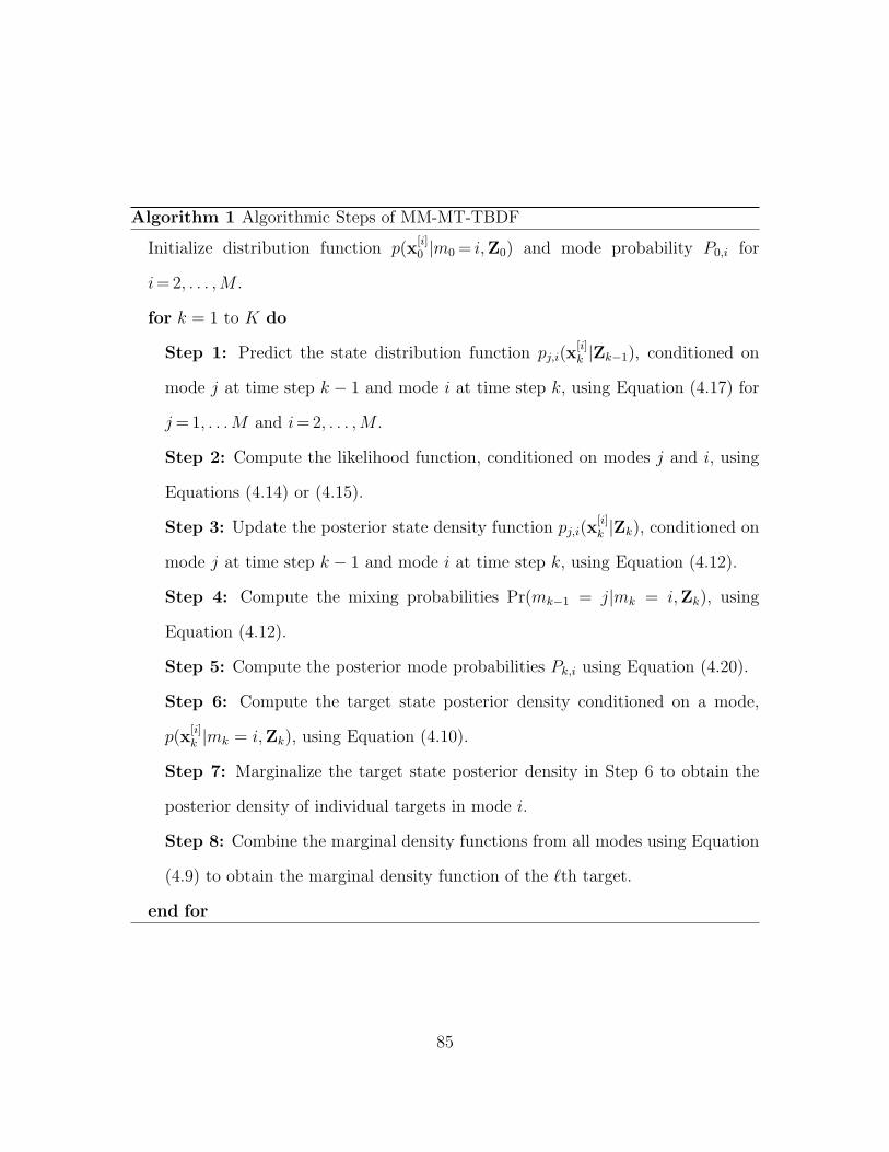
Algorithm 1 Algorithmic Steps of MM-MT-TBDF

Initialize distribution function p(x[i]0 |m0= i,Z0) and mode probability P0,i for

i=2, . . . ,M .

for k = 1 to K do

Step 1: Predict the state distribution function pj,i(x[i]k |Zk−1), conditioned on

mode j at time step k − 1 and mode i at time step k, using Equation (4.17) for

j=1, . . .M and i=2, . . . ,M .

Step 2: Compute the likelihood function, conditioned on modes j and i, using

Equations (4.14) or (4.15).

Step 3: Update the posterior state density function pj,i(x[i]k |Zk), conditioned on

mode j at time step k − 1 and mode i at time step k, using Equation (4.12).

Step 4: Compute the mixing probabilities Pr(mk−1 = j|mk = i,Zk), using

Equation (4.12).

Step 5: Compute the posterior mode probabilities Pk,i using Equation (4.20).

Step 6: Compute the target state posterior density conditioned on a mode,

p(x[i]k |mk = i,Zk), using Equation (4.10).

Step 7: Marginalize the target state posterior density in Step 6 to obtain the

posterior density of individual targets in mode i.

Step 8: Combine the marginal density functions from all modes using Equation

(4.9) to obtain the marginal density function of the ℓth target.

end for

85

Pr(mk =2| Zk)

Compute

p(xk[M] | mk-1 = 2, mk = M, Zk)

Compute

p(xk[M] | mk-1 =M, mk = M, Zk)

Compute

p(xk[M] | mk-1 = 1, mk = M, Zk)

Compute

p(xk[2] | mk-1 = 2, mk = 2, Zk)

Pr(mk-1 =1 | mk=2, Zk)

Pr(mk-1 =2 | mk=2, Zk)

Pr(mk-1 =M | mk=2, Zk)

Compute

p(xk[2] | mk-1 = 1, mk = 2, Zk)

Pr(mk-1 =1 | mk=M, Zk)

Pr(mk-1 =2 | mk=M, Zk)

Pr(mk-1 =M | mk=M, Zk)

Compute

p(xk[2] | mk-1 = M, mk = 2, Zk)

p(xk[2] | mk=2, Zk)

p(xk[M] | mk=M, Zk)

p(xk[M], mk=M| Zk)

p(xk[2], mk=2| Zk)

Pr(mk =M| Zk)

Figure 4.1: MM-MT-TBDF Algorithm Block Diagram for Multiple Target Tracking.

Thus, the detection of a new target is tracked by observing the mode probabilities

and a newly detected target and its corresponding trajectory is implicitly labelled

through the corresponding mode definition. Figure 4.2 illustrates our method with

an example scenario in which L = 2 targets enter and leave the FOV at different time

steps. The figure shows only the dominant probabilities corresponding to the different

mode transitions and the PDFs corresponding to these dominant probabilities.

86

No

Targets

Pr(1|2, Zk)

Pk,3, Pr(ek,2|Zk), k[3], k,2

Pk,2,

Pr(ek,1|Zk),

k[2], k,1

Pk,4,

Pr(ek,1|Zk),Pr(ek,2|Zk),

k[4], k,1, k,2

Pr(2|2, Zk)

Pr(2|4, Zk) Pr(4|4, Zk)

Pr(4|3, Zk)

Pr(3|4, Zk)

Pr(2|1, Zk)

Pr(4|3, Zk)

Pr(3|3, Zk)

Pr(1|1,Zk)

Pr(4|4, Zk)

Pr(2|2, Zk)

Pk,1

Figure 4.2: Illustration of MM-MT-TBDF Algorithm for L = 2 Targets Showing

the Dominant Probabilities and the Relevant Posterior PDFs for Different Mode

Transitions.

4.4 Particle Filter Implementation of Multiple Mode Multiple Target TBDF

In the previous section, we derived the Bayesian solution of the MM-MT-TBDF

algorithm. When the state and measurement models are nonlinear and non-Gaussian,

then the TBDF needs to be solved using sequential Monte Carlo (SMC) techniques

such as particle filtering. Unlike the multiple model TBDF in [101], we employ two

layers of IMM structure to derive the posterior PDF. The first layer of IMM structure

is used to estimate the mode conditioned PDF and the second layer is used to estimate

the PDF of the target state vector. The particle filter (PF) based implementation

(MM-MT-TBDF-PF) is also proposed to implement the MM-MT-TBDF algorithm.

87

The proposed algorithm employs three layers of particle filters. The first layer of PFs

approximate the posterior PDF of target states x[i]k , conditioned on mode i at time

step k and mode j at time step k − 1. This approximation is given by

p(x[i]k |mk−1 = j,mk = i,Zk) ≈

Nj,i∑n=1

ϕ(j,i,n)k δ(x

[i]k − x

(j,i,n)k ) . (4.21)

The next layer of PFs approximating the mode conditioned posterior PDFs are given

by

p(x[i]k |mk = i,Zk) ≈

Ni∑n=1

χ(i,n)k δ(x

[i]k − x

(i,n)k ) . (4.22)

The final layer of PFs approximates the posterior PDF of individual targets as

p(xk,ℓ|Zk) ≈Nℓ∑n=1

w(n)k,ℓ δ(xk,ℓ − x

(n)k,ℓ ). (4.23)

4.4.1 MM-MT-TBDF Using Sampling Importance Resampling Particle Filter

We begin this algorithm by initializing the particles x(i,n)0 and weights χ

(i,n)0 ,

i=2, . . . ,M for all modes. At time step k, Nj,i new particles are generated to ap-

proximate p(x[i]k |mk−1 = j,mk = i,Zk), for all i and j. The samples are generated

depending on whether or not a particular target is present in the previous mode.

There are three possible target transitions.

• Target enters the FOV:

If a target in mode i was not present in mode j, then this target is considered

as a target that entered the FOV at time step k and the particles are gener-

ated based on a known a priori distribution for a new target. If no a priori

information about a new target is available, a uniform distribution can be as-

sumed. Specifically, the target position particles can be drawn uniformly from

the FOV, and the target state velocity particles can be drawn from a uniform

88

distribution whose range values are the expected minimum and maximum tar-

get velocities. The target intensity particles can also be drawn from a uniform

distribution whose range values are selected based on the expected peak SNR in

the measurement. Since the proposed algorithm is for tracking multiple targets,

the position vector cannot be simply sampled from the FOV in order to avoid

drawing samples in the vicinity of the already detected target position. To avoid

this problem, samples in the neighbourhood of the already detected target are

not selected. One optimal way is to compute the Mahalanobis distance between

the generated particles and the mean position of the already detected targets.

The Mahalanobis distance is calculated as

D(xk−1,d,xk,ℓ) = (x(n)k,ℓ − µd

k−1)T Sd

k−1 (x(n)k,ℓ − µd

k−1)

where d is the already detected target with sample mean position estimate vec-

tor µdk−1 and corresponding sample position covariance estimate matrix Sd

k−1 at

time step k − 1, x(n)k,ℓ is the position vector of the generated particles for target

ℓ. It was shown in [54] that a lower number of particles are needed if the sam-

ples are generated directly from the measurement. However, we observed that

selecting a subset of measurements by thresholding does not work well under

low SNR conditions. For best performance, we propose a balanced approach in

which a large number (Nnb) of uniformly distributed new target particles are

used. The likelihood function for this large set of particles is computed first and

the Nj,i highest likelihood particles are selected from this large set. Following

this procedure helps to localize the computation only during the new target

particle generation rather than propagating a large set of particles through the

remaining steps described below. Even though the likelihood function compu-

tation monotonically involves the measurements, choosing a higher amplitude

89

measurement bin may not necessarily result in a higher likelihood function value

since the likelihood function is also a function of the neighbourhood bins. From

our simulations, we noted that choosing state vectors corresponding to higher

amplitude measurement bins resulted in poor performance at lower SNR con-

ditions (less than 0 dB SNR) since most of the chosen higher amplitude bins

corresponded to noise spikes. If a priori information is available as in [75], then

a reduced number of initial particles are needed.

• Target leaves FOV:

A target has left the FOV if it is present in mode j but not in mode i. The

particles corresponding to this target at time step k in mode i are ignored.

• Target remains in FOV:

If a target is already present in the FOV during mode j and remains in the FOV

during mode i, then the particles for pj,i(x[i]k |Zk) are updated using Equation

(4.2).

Finally, the states of all the targets that are present in mode i are then concatenated

to approximate pj,i(x[i]k |Zk−1).

The weights for the Nj,i particles are computed using the mode conditioned joint

likelihood function in Equation (4.15) as

ϕ(j,i,n)k ∝ L(zk|x(j,i,n)

k ,mk−1 = j,mk = i)p(x

(j,i,n)k |y(i,n)

k−1 ,Zk)

q(x(j,i,n)k |y(i,n)

k−1 ,Zk)

where y(i,n)k−1 is the set of particles corresponding to mode i at time step k− 1 derived

by collating particles corresponding to mode j at time step k − 1. If the targets are

assumed to move independently, the above weight calculation can be written as

ϕ(j,i,n)k ∝ L(zk|x(j,i,n)

k ,mk−1 = j,mk = i)

Li∏ℓ=1

p(x(j,i,n)k,ℓ |y(i,n)

k−1,ℓ,Zk)

q(x(j,i,n)k,ℓ |y(i,n)

k−1,ℓ,Zk)(4.24)

90

where Li is the number of targets in mode i. The weights are normalized by

Λ′

j,i =

Nj,i∑n=1

ϕ(j,i,n)k (4.25)

to obtain ϕ(j,i,n)k = ϕ

(j,i,n)k /Λ

′j,i and Λ

′j,i is the particle approximation of Λj,i in Equa-

tions (4.13) and (4.20). Given the initial mode probability P0,i, for all i, the mixing

probabilities in Equation (4.18) are then calculated as

Pr(mk−1 = j|mk = i,Zk) =Λ

′j,i Ωj,i Pk−1,j

M∑j′=1

Λ′

j′,i Ωj′,i Pk−1,j′

. (4.26)

The mode conditioned PDF in Equation (4.25) can be approximated as

p(x[i]k |mk = i,Zk) ≈

M−1∑j=0

Nj,i∑n=1

Pr(j, i)ϕ(j,i,n)k δ(x

[i]k − x

(j,i,n)k ) . (4.27)

The number of particles representing p(x[i]k |mk = i,Zk) is equal to the sum of the

particles representing each mode transition. In order to reduce the computational

complexity, the weights of the above particles are sorted and the Ni highest weights

with their corresponding particles are selected. The sorted weights are then normal-

ized and resampled to obtain χ(i,n)k . The mode conditioned probability can then be

approximated as in Equation (4.25). Note that the particles x(i,n)k are resampled to

avoid sample degeneracy [15]. The marginal mode conditioned posterior PDF of the

ℓth target p(xk,ℓ|Zk) is obtained by selecting particles corresponding to that particular

target i.e.,

p(x[i]k,ℓ|mk = i,Zk) ≈

Ni∑n=1

χ(i,n)k δ(x

[i]k,ℓ − x

(i,n)k,ℓ ) .

The mode probabilities are computed using Equation (4.20) by substituting Λ′j,i for

Λj,i. The mode probability corresponding to no targets being present is obtained by

91

subtracting the sum of the probabilities of other modes from 1, i.e.,

Pk,0 = 1−M∑i=2

Pk,i.

Finally, the particles corresponding to all the modes that include the ℓth target are

combined and weighted accordingly, based on the mode probability. Specifically,

p(xk,ℓ|Zk) ≈M∑i=2

Ni∑n=1

CiℓPk,iχ

(i,n)k δ(x

[i]k,ℓ − x

(i,n)k,ℓ ) . (4.28)

As mentioned above, during the mixing process, the number of particles representing

p(xk,ℓ|Zk) is equal to the sum of the particles representing each mode. The weights

of the above particles are sorted and the Nℓ highest weights with their corresponding

particles are selected. The sorted weights are then normalized and resampled to get

w(n)k,ℓ which will be used in approximating p(xk,ℓ|Zk) as in Equation (4.23). The target

existence probability of the ℓth target is obtained by summing up the relevant mode

probabilities as

Pr(ek,ℓ|Zk) =M∑i=2

CiℓPk,i . (4.29)

The PF implementation steps of the MM-MT-TBDF algorithm are summarized in

Algorithm 2.

92

Algorithm 2 Algorithmic Steps of MM-MT-TBDF-PF

Initialize the particle distribution of p(x[i]0 |m0 = i,Z0) and mode probability P0,i

for i=2, . . . ,M

for k = 1 to K do

Step 1: Predict the particle distribution for pj,i(x[i]k |Zk−1), conditioned on mode

j at time step k − 1 and mode i at time step k for j=1, . . .M and i=2, . . . ,M

• Particles for new targets entering the FOV:

x(n)k,nb ∼ q(x

(j,i,n)k,ℓ ), n = 1, . . . , Nnb, Nnb ≫ Nj,i , ℓ = 1, . . .Li

Compute the likelihood function L(Zk|x(n)k,nb)

Pick Nj,i highest likelihood particles and set them to x(j,i,n)k,ℓ

• Particles for targets remaining in the FOV:

x(j,i,n)k,ℓ ∼ p(x

(j,i,n)k,ℓ |y(i,n)

k−1,ℓ) n = 1, . . . , Nj,i, ℓ = 1, . . .Li,

• Concatenate the new particles to get x(j,i,n)k

Step 2: Compute the joint likelihood function, conditioned on modes j and i,using Equation (4.15)

Step 3: Compute the weights ϕ(j,i,n)k Ni,j

n=1 as in Equation (4.24) as a function ofthe proposal density function

Step 4: Compute the cumulative weights Λ′j,i using Equation (4.25)

Step 5: Normalize the weights ϕ(j,i,n)k Ni,j

n=1

Step 6: Compute the mixing probabilities Pr(mk−1 = j|mk = i,Zk) usingEquation (4.26)

Step 7: Update the mode conditioned posterior PDF, p(x[i]k |mk = i,Zk), using

Equation (4.27)

Step 8: Pick Ni highest weights and normalize the weights to get χ(i,n)k Ni

n=1

Step 9: Resample the normalized weights to get x(i,n)k

Step 10: Marginalize the posterior PDF to get x(i,n)k,ℓ , ℓ=1, . . . ,Li

Step 11: Compute the posterior mode probabilities Pk,i using Equation (4.20)

Step 12: Compute the individual target state posterior PDF p(xk,ℓ|Zk), usingEquation (4.28)

Step 13: Pick Nℓ highest weights and normalize the weights to get w(n)k,ℓ

Nℓn=1

Step 14: Resample the normalized weights to get x(n)k,ℓ , ℓ=1, . . . ,L

Step 15: Compute the target existence probability using Equation (4.29)

end for

93

4.5 Simulations

In all our simulations involving multiple targets, the optimal sub-pattern assign-

ment (OSPA) metric [105] is used to compare the tracking performances of various

methods. We have used the OSPA metric over the standard root mean-squared er-

ror (RMSE) metric to properly quantify the overall algorithm performance in terms

of target cardinality error and localization error. The cardinality error quantifies the

number of times the algorithm missed detecting an existing target or falsely detecting

a non-existent target. The localization error quantifies how well the tracker follows

the true target location.

4.5.1 Tracking Three Targets Using Image Measurements

In this section, we demonstrate the performance of the proposed MM-MT-TBDF

algorithm for a 2-D image measurement to track three targets using the same set

of measurement parameters used by the authors in [67]. The measurement is gen-

erated using a constant velocity target motion model and additive Gaussian process

noise. The covariance matrix Q for the noise vk for a discrete-time equivalent of a

continuous-time model of constant velocity target motion [93] is given by

Q =

q1∆T 3

3

q1∆T 2

20 0 0

q1∆T 2

2q1∆T 0 0 0

0 0q1∆T 3

3

q1∆T 2

20

0 0q1∆T 2

2q1∆T 0

0 0 0 0 q2∆T

(4.30)

where q1 and q2 are the process noise parameters for the target motion and intensity

respectively and ∆T =1 s. The process noise parameters were selected as q1=0.0001,

q2=0.01 and the measurement noise variance was r=1. The measurement frames

94

were generated at different SNR conditions: 19.8, 16.3, 13.8 and 10.2 dB with the

corresponding intensity value of I0,ℓ=30, 20, 15, 10, respectively for all ℓ. Twenty

five frames of measurements were generated with the following parameters, x=1,

y =1, Nx=20, Ny =20, blurring parameter Σ=0.7. The measurements are gener-

ated such that the first target appeared in the first frame and left in the 21st frame.

The second and third targets appeared in the 5th and 11th frames, respectively, and

stayed in the FOV during the remainder of the measurement frames. The initial

kinematic state vectors were [14.2 -0.1 7.2 0.1], [6.2 0.0 4.0 0.1] and [0.0 0.1 10.2 0.12]

for Targets 1, Target 2, and Target 3, respectively. Figures 4.3(a) and 4.3(b) show

the measurements from frame 15 at 19.8 dB and 10.2 dB peak SNR, respectively.

Note that the targets are barely visible at 10.2 dB peak SNR. The parameters used

in the generation of new target particles are νmax=−1 and νmin=1, Imin= I0,ℓ − 5,

Imax= I0,ℓ +5. The probabilities in Equation (4.4) are PB =0.01 and PD =0.02. The

number of neighborhood pixels used for the calculation of the likelihood function in

Equation (4.14) is set 3. The number of the particles in this simulation is set to

10,000 for all layers of particles filters, that is Nj,i, Ni and Nℓ for all i, j and ℓ. The

number of particles for new targets, Nnb is also set at 10,000.

Figure 4.4(a) shows the corresponding probability of target existence for all three

targets indicating the latency involved in detecting the target mode transitions. In

general, for all targets, as the SNR decreases, the detection latency increases. Figure

4.4(b) shows the OSPA tracking error with the OSPA parameter set to c=40 and

p=2 at 19.8 dB, 16.3 dB, 13.8 dB and 10.2 dB peak SNR. The cardinality and

the localization error is very small at 19.8 dB and 16.3 dB. Note that when the

cardinality error is very small, it is shown that the algorithm correctly tracks the

number of existing targets without any false detection. The cardinality error at 13.8

dB SNR is slightly high indicating that there is a one frame delay in detecting when

95

05

1015

20

0

5

10

15

20−5

0

5

10

x coordinate

Frame :15

y coordinate

Nor

mal

ized

Inte

nsity

(a)

05

1015

20

0

5

10

15

20−4

−2

0

2

4

x coordinate

Frame :15

y coordinate

Nor

mal

ized

Inte

nsity

(b)

Figure 4.3: Measurement Frames: (a) Time Step 15, 19.8 dB Peak SNR. (b) Time

Step 15, 10.2 dB Peak SNR

Target 2 enters the FOV around the 5th frame. Similarly at 10.2 dB SNR, there was a

two-frame delay in detecting when the third target entered the FOV around the 11th

frame. This latency trend is also evident from the probability of target detection in

Figure 4.4(a). Despite the delay in detecting a target, the localization error at lower

SNR is still good, confirming the excellent performance of our proposed algorithm

under lower SNR measurement conditions.

4.5.2 Tracking Three Targets Using Radar Measurements

For the radar simulations, we used the OSPA parameters p=2 and c=16. The

value of the cut-off parameter c=16 provides a good balance between the localization

and the cardinality error. Moreover, the FOV in our simulations is in the same

order of magnitude as the cut-off parameter. In this measurement model, we assume

constant velocity and Gaussian noise models with the covariance matrix of the state

transition matrix defined in Equation (4.30). The process noise variance parameters

are q1= 0.01 and q2=0.001. The tracking FOV is [0 16.97] m in both the x and

y direction. Measurements from two sensors located at (0, 0) and (0, 16.97) m are

96

0 5 10 15 20 250

0.2

0.4

0.6

0.8

1

1.2

1.4

Time, k

Pro

babi

lity

of ta

rget

exi

sten

ce

Pe Vs Time for various SNR

snr=19.8 dB, Tgt. 1snr=16.3 dB, Tgt. 1snr=13.8 dB, Tgt. 1snr=10.2 dB, Tgt. 1snr=19.8 dB, Tgt. 2snr=16.3 dB, Tgt. 2snr=13.8 dB, Tgt. 2snr=10.2 dB, Tgt. 2snr=19.8 dB, Tgt. 3snr=16.3 dB, Tgt. 3snr=13.8 dB, Tgt. 3snr=10.2 dB, Tgt. 3

(a)

0 5 10 15 20 2510

−2

10−1

100

101

102

k

OS

PA

(40,

2)

OSPA, c = 40, p = 2

SNR = 19.8 dBSNR = 16.3 dBSNR = 13.8 dBSNR = 10.2 dB

(b)

Figure 4.4: Image Measurement Case: (a) Target Existence Probability (Red Circles,

Blue Stars and Black Triangles Indicate the Frames at which Target 1, Target 2

and Target 3 Truly Exist, respectively); and (b) Tracking Error at Different SNR

Conditions, OSPA(40,2).

used in our simulations. A single measurement frame consists of (48 × 48 × 48) bins

resulting in the following measurement bin resolutions, range ∆r =0.509 m, range-

rate ∆r =0.0766 m/s, and azimuthal angle ∆θ =0.0334 radians. The corresponding

measurement ranges are: range [0 24) m, range-rate [-1.8 1.8) m/s and azimuthal

angel [0 π/2) radians for sensor 1 and (−π/2 0] radians for sensor 2. The spread

factors used in the measurement models are: σr =1.1 m , σr =0.35 m/s, σθ =0.06

radians. The measurement noise variance νk is set to 1. Therefore, the peak SNR

corresponding to the ℓth target is calculated as

SNRpeak =[∆r∆r∆θIk,ℓ]

2

((2π)3/2σrσrσθ)2νk. (4.31)

The expected target component velocity range is set to [-1 1] m/s, and the expected

peak SNR range is set to [-3 6] dB. We used low SNR conditions for all our simulations

to demonstrate that the proposed algorithm can work under difficult environmental

conditions. It is important to note that the proposed algorithm can also be used

97

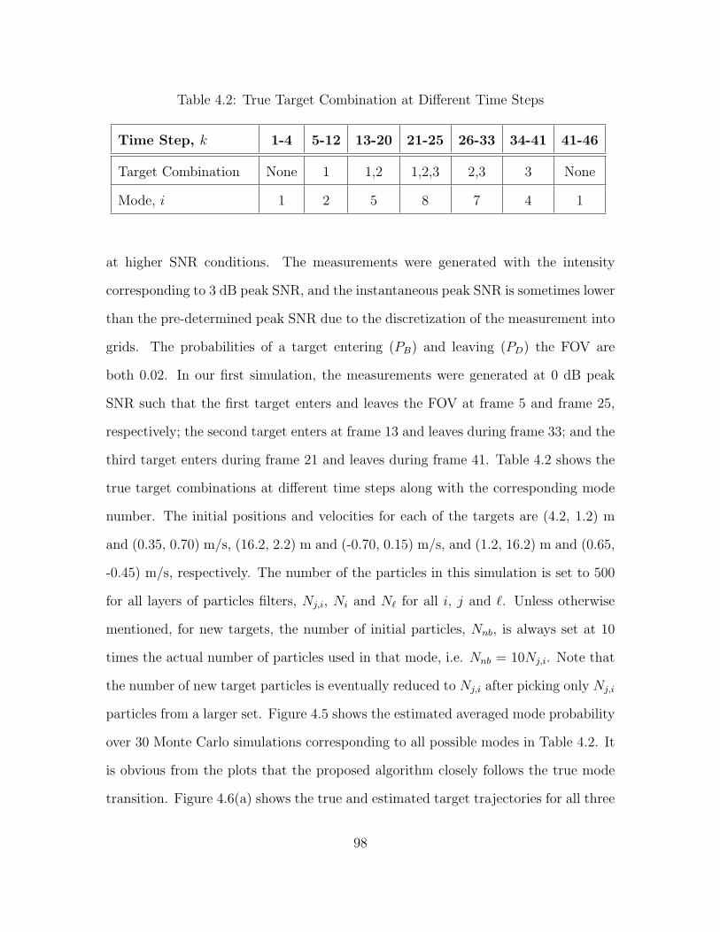
Table 4.2: True Target Combination at Different Time Steps

Time Step, k 1-4 5-12 13-20 21-25 26-33 34-41 41-46

Target Combination None 1 1,2 1,2,3 2,3 3 None

Mode, i 1 2 5 8 7 4 1

at higher SNR conditions. The measurements were generated with the intensity

corresponding to 3 dB peak SNR, and the instantaneous peak SNR is sometimes lower

than the pre-determined peak SNR due to the discretization of the measurement into

grids. The probabilities of a target entering (PB) and leaving (PD) the FOV are

both 0.02. In our first simulation, the measurements were generated at 0 dB peak

SNR such that the first target enters and leaves the FOV at frame 5 and frame 25,

respectively; the second target enters at frame 13 and leaves during frame 33; and the

third target enters during frame 21 and leaves during frame 41. Table 4.2 shows the

true target combinations at different time steps along with the corresponding mode

number. The initial positions and velocities for each of the targets are (4.2, 1.2) m

and (0.35, 0.70) m/s, (16.2, 2.2) m and (-0.70, 0.15) m/s, and (1.2, 16.2) m and (0.65,

-0.45) m/s, respectively. The number of the particles in this simulation is set to 500

for all layers of particles filters, Nj,i, Ni and Nℓ for all i, j and ℓ. Unless otherwise

mentioned, for new targets, the number of initial particles, Nnb, is always set at 10

times the actual number of particles used in that mode, i.e. Nnb = 10Nj,i. Note that

the number of new target particles is eventually reduced to Nj,i after picking only Nj,i

particles from a larger set. Figure 4.5 shows the estimated averaged mode probability

over 30 Monte Carlo simulations corresponding to all possible modes in Table 4.2. It

is obvious from the plots that the proposed algorithm closely follows the true mode

transition. Figure 4.6(a) shows the true and estimated target trajectories for all three

98

5 10 15 20 25 30 35 40 450

0.2

0.4

0.6

0.8

1

Frame Number

Mod

e P

roba

bilit

y

P

k,0P

k,1 Pk,4 P

k,7P

k,6 Pk,3

Pk,0

Figure 4.5: Mode Probability for Three Targets at 3 dB Peak SNR.

targets in all Monte Carlo simulations. Initially the estimated target location deviates

from the true location, however, the estimated target location converged to the true

location as more measurements were received. Figure 4.6(b) shows the corresponding

OSPA averaged over 30 Monte Carlo simulations. The cardinality error dominates

the OSPA during the true mode transitions at frames 13, 21, 26, 33 that correspond

to the target events: appearance of Target 2, appearance of Target 3, disappearance

of Target 1 and disappearance of Target 3, respectively. The localization error is in

general very small, around 0.3 m.

99

0 2 4 6 8 10 12 14 160

2

4

6

8

10

12

14

16

Target 1 Start

x co−ordinate

y co

−or

dina

te


Target 2 Start

Target 3 Start True

(a)

0 10 20 30 40 500

0.5

1

1.5

2

2.5

3

k

OS

PA

(16,

2)

OSPA, c = 16, p = 2

(b)

Figure 4.6: Radar Measurement Tracking of Three Targets at 3 dB Peak SNR: (a)

True and Estimated Target Trajectories (Solid Lines Represent the True Target Tra-

jectory and Red Circles, Blue Stars and Black Triangles Represent the Estimated

Trajectory of Target 1, Target 2 and Target 3 respectively; and (b) Tracking Error,

OSPA(16,2).

100

Chapter 5

EFFICIENT IMPLEMENTATION OF MULTIPLE TARGET

TRACK-BEFORE-DETECT FILTERING

5.1 Computational Issues of the Multiple Mode Multiple Target

Track-before-detect Filter

In Chapter 4, we proposed the multiple mode multiple target track-before-detect

filter (MM-MT-TBDF), and we discussed its particle filter (PF) implementation

(MM-MT-TBDF-PF). The proposed algorithm suffers from the curse of dimension-

ality when the maximum number of targets increases. In this chapter, we propose a

partitioning based method to mitigate the curse of dimensionality problem thereby

improving the tracking performance for a given number of particles. This method par-

titions the multi-target space into a single target space to generate proposal particles

and then uses the measurement to select only highly likelihood particles from a set

of particles generated from the single target space partition. The proposal particles

generated this way result in greatly improving the tracking performance. The Markov

chain Monte Carlo (MCMC) step using the Metropolis-Hastings method [17] is also

integrated into the proposal particle generation step to reduce sample impoverish-

ment. The number of target combinations can grow exponentially as the maximum

number of targets increases. To mitigate the effects of curse of dimensionality, we

propose a heuristical decision-directed based approach to keep the computational

complexity of the algorithm as a linear function of the maximum number of targets.

101

5.2 Proposal Function Using PF Partition Method

The performance of the PF based algorithm can suffer if the same number of

particles is assigned for all possible modes in the MM-MT-TBDF-PF. For example, a

mode with three targets uses the same number of particles as a mode with only one

target even though the number of parameters to be estimated in the first case is three

times higher than the latter case. Assigning the same number of particles to all the

modes can become a problem when the dimensionality of the multi-target state vector

increases. This problem can be avoided by assigning different number of particles to

different modes. However, the total number of particles can grow significantly as

the number of targets that are assumed present in a mode increases. Moreover, the

amount of computations necessary to run different PFs for all the modes increases

drastically since the combinatorial complexity increases exponentially as a function

of the total number of targets. In this chapter, we propose a method that is based

on state space partitioning to reduce the number of particles in order to reduce the

overall computational complexity. Since the number of modes can grow exponentially

as a function of the maximum number of targets, even a small decrease in the number

of particles can have an overall impact on the computational performance.

In [106], a method was proposed to estimate the joint multi-target probability

density function (PDF) to track an unknown number of targets; the method intro-

duced different proposal functions by partitioning the single target state space and

illustrated that a fewer number of particles (orders of magnitude smaller) were re-

quired. The computational complexity was reduced by incorporating information

from measurements into the proposal function. Our proposed MM-MT-TBDF parti-

tioning (MM-MT-TBDF-IP) also uses measurement information during the particle

generation step for the posterior PDF conditioned on mode i at time k and mode j

102

at time k− 1. We use the simplified form of the sequential partitioning algorithm by

exploiting the fact that the number of assumed targets in a mode is known. In most

cases, the number of partitions needed is then equal to the number of targets. In

[106], three different partitioning methods were proposed: independent, coupled and

adaptive partitioning. Our proposed algorithm can incorporate all three methods.

Without loss of generality, in what follows, we only describe the independent parti-

tioning (IP) method. The coupled and adaptive partitioning methods can be used if

the targets are moving close to each other.

The sequential partitioning algorithm [106, 107] has five major steps: partition

sampling, partition weight computation, resampling of partition weights, particle

weights computation and resampling of particles. In Chapter 4, Section 4.4.1, the

predicted density function conditioned on the current and previous mode pj,i(xik|Zk−1)

was approximated using the particles for targets entering the field of view (FOV) and

remaining in the FOV. Using the IP method, the likelihood function corresponding to

the predicted particles for each target in a mode is computed. The likelihood function

for each target is termed the partition weights α(j,i,n)k,l in [106], and i, j are the mode

numbers at time steps k and (k− 1), respectively and n is the corresponding particle

number of the partition weight. The partition weights are normalized and resampled

to generate a new set of predicted particles. The new particles closely approximate

the true underlying density function since the density also incorporates the measure-

ment information. If we assume that the targets are moving independently, the joint

proposal function can be written as

q(x(j,i,n)k |y(j,i,n)

k−1 ,Zk) =

Li∏ℓ=1

q(x(j,i,n)k,ℓ |y(j,i,n)

k−1,ℓ ,Zk) (5.1)

where Li is the number of targets in mode i. Since the proposal function is now

also a function of the measurement likelihood, the proposal density function for each

103

target that will be used in Equation (4.24) can be written as [107]

q(x(j,i,n)k,ℓ |y(j,i,n)

k−1,ℓ ,Zk) =

α(j,i,n)k,l q(x

(j,i,n)k,ℓ ), target entering FOV

α(j,i,n)k,l p(x


k−1,ℓ), target remaining in FOV

where p(x(j,i,n)k,ℓ |y(i,n)

k−1,ℓ) is the posterior PDF conditioned on modes at time steps k and

(k− 1) and it is represented by a PF in Equation (4.21), whose weights are obtained

using Equation (4.24), y(i,n)k−1,ℓ is the ℓth target’s state vector corresponding to mode j

at time step (k− 1) that is transformed to mode i using Equation (4.16) and x(i,n)k,ℓ is

the particle corresponding to the ℓth target’s partition for the corresponding modes

i and j at time steps k and (k − 1), respectively. The implementation steps of the

IP method that replace Step 1 and Step 3 of Algorithm 2, respectively, are shown in

Algorithm 3.

104

Algorithm 3 PF Proposal Steps Using Independent Partitioning Method

Step 1: Predict the particle distribution for pj,i(x[i]k |Zk−1), conditioned on mode j

at time k − 1 and mode i at time k for j=0, 1, . . .M − 1 and i=1, . . . ,M − 1.

• Particles for new targets entering the FOV:

x(j,i,n)k,nb ∼ q(x

(j,i,n)k,ℓ ), n = 1, . . . , Nnb, Nnb ≫ Nj,i, ℓ=1, . . . ,Li

• Particles for targets remaining in the FOV:

x(j,i,n)k,ℓ ∼ p(x


k−1,ℓ) n = 1, . . . ,Nj,i, ℓ=1, . . . ,Li

• Compute partition weights:

Particles for new targets entering the FOV: α(j,i,n)k,l ∝ p(Zk|x(j,i,n)

k,nb )

Pick only Nj,i highest likelihood particles and set them to x(j,i,n)k,ℓ

Particles for targets remaining in the FOV: α(j,i,n)k,l ∝ p(Zk|x(j,i,n)

k,ℓ )

• Normalize partition weights:

α(j,i,n)k,l =

α(j,i,n)k,l∑Nj,i

n=1 α(j,i,n)k,l

• Resample the normalized particles to obtain x(j,i,n)k,ℓ and α

(j,i,n)k,l

• Concatenate the new particles from all partitions to obtain x(j,i,n)k

Step 3: Compute the particle weights using the proposal function in Equation

(5.1),

• ϕ(j,i,n)k =

L(zk|x(j,i,n)k ,mk−1 = j,mk = i)

Nj,i

∏Li

ℓ=1 α(j,i,n)k,l

105

5.3 MM-MT-TBDF-IP with Markov Chain Monte Carlo

Sample impoverishment is a common problem with particle filters, especially when

the process model noise variance is small [16]. This is the result of lack of sample

diversity during the generation of predicted particles. There exist many methods to

mitigate the problem of sample impoverishment [17], [16]. We used the Markov Chain

Monte Carlo (MCMC) approach to increase sample diversity without affecting the es-

timated posterior density function. Specifically, we used the Metropolis-Hastings [17]

algorithm to perform the resample-move operation (MM-MT-TBDF-IP-MCMC). As

shown in the previous section, the particles approximating the posterior density func-

tion conditioned on the current and previous mode are resampled to obtain x(j,i,n)k .

The covariance of this distribution can be estimated from the current particle dis-

tribution. In order to improve the sample diversity, a perturbation is added to the

existing particles by adding new samples that are drawn from a Gaussian distribu-

tion with zero mean and the covariance equal to the one estimated from the particle

distribution. The conditional sample move operation is then performed based on the

likelihood ratio of the particles before and after the addition of the perturbation. The

Metropolis-Hastings sample move step is performed only for surviving targets. With

out the Metropolis-Hastings step, the remaining MCMC steps simply constitute the

regularized particle filter [17]. This MCMC step is performed after Step 5 in Algo-

rithm 2 as a new Step 5a. The MCMC steps used in our algorithm are summarized

in Algorithm 4.

106

Algorithm 4 Metropolis-Hasting Steps for MM-MT-TBDF-IP-MCMC

Step 5a:

• For a target that survives from previous time step, compute the posterior

covariance matrix Sℓ from the predicted particle distribution x(j,i,n)k,ℓ . For a

new target entering the FOV, set the covariance matrix to some pre-defined

value, Sℓ = Snb.

• Obtain samples from the Gaussian random process, ϵ ∼ N (0, Sℓ). Use the

random process ϵ to add a perturbation to the resample particles.

• Add some jitter to the already resampled particles x(j,i,n)k,ℓ = x

(j,i,n)k,ℓ +hoptS

1/2ℓ ϵ

where hopt = 0.9397( 1Nj,i

)1/9, the various constants are described in [16, 17].

• Compute the Metropolis-Hastings acceptance probability,

β = min

1,

p(Zk|x(j,i,n)k,ℓ )p(x


k−1,ℓ)

p(Zk|x(j,i,n)k,ℓ )p(x


k−1,ℓ)

.

• for n = 1:Nj,i

Draw a number u ∼ U [0 1]

A resampled particle x(j,i,n)k,ℓ is moved to a new location x

(j,i,n)k,ℓ only if u ≤ β

end

107

5.4 Simulations

5.4.1 Tracking Three Targets Using Radar Measurements

In the first simulation, we analyze the tracking result of the MM-MT-TBDF-

IP-MCMC method for the simulation used in Section 4.5.2. Figure 5.1 shows the

estimated averaged mode probability at different frames over 30 Monte Carlo simu-

lations. The mode probability values are more accurate when compared to the mode

5 10 15 20 25 30 35 40 450

0.2

0.4

0.6

0.8

1

Frame Number

Mod

e P

roba

bilit

y

P

k,0P

k,1 Pk,4 P

k,7P

k,6P

k,3 Pk,0

Figure 5.1: Mode Probability for Three Targets at 3 dB Peak SNR (MM-MT-TBDF-

IP-MCMC).

probability obtained using the MM-MT-TBDF-PF method in Figure 4.5. For exam-

ple, the mode probability value when Targets 2 and 3 are present is higher with the

partitioning method, and it takes longer for the other method to detect the presence

of all three targets. Figure 5.2 shows the true and estimated target trajectories for all

three targets in all Monte Carlo simulations. The variance of the target position es-

timate is much smaller when compared to the MM-MT-TBDF-PF method in Figure

108

4.6(a). The faster convergence rate of the target position estimate with the partition-

ing method is evident from the target position estimate in the vicinity of its initial

position. Figure 5.3 shows the corresponding OSPA averaged over 30 Monte Carlo

0 2 4 6 8 10 12 14 160

2

4

6

8

10

12

14

16

Target 1 Start

x co−ordinate

y co

−or

dina

teTarget position estimate

Target 2 Start

Target 3 Start True

Figure 5.2: True and Estimated Target Trajectories for Three Targets at 3 dB Peak

SNR.

simulations with 500 particles. The cardinality error dominates the OSPA when the

first target appears at frame 5, second target appears at frame 13 and also when the

third target appears at frame 21, implying that once in a while, there is a one frame

latency in detecting a new target that enters the FOV. The OSPA also shows that

the algorithm is able to quickly detect a target leaving the FOV since the OSPA value

is low at frames 25, 33 and 41. The localization error is around 0.1 m. The figure

also shows the OSPA with different number of particles along with the one from the

MM-MT-TBDF-PF method. For the same number of particles, the localization error

109

using the partition method is three times smaller than the other method. In other

words, the MM-MT-TBDF-IP-MCMC method needs a smaller number of particles to

achieve similar tracking performance as the MM-MT-TBDF-PF method. This is evi-

dent with the OSPA for 100 and 50 particles in Figure 5.3 where the tracking error is

in the same order as for the MM-MT-TBDF-PF method. This result agrees with the

findings in [106] that the regular PF method needs an order of magnitude higher num-

ber of particles than the IP method to achieve similar tracking error. The averaged

OSPA with the IP method is higher at a lower process model variance. Therefore,

partitioning the target state space helps us to achieve better tracking performance

while reducing the required number of particles.

0 5 10 15 20 25 30 35 40 4510

−2

10−1

100

101

k

OS

PA

(16,

2)

OSPA, c = 16, p = 2

MM−MT−TBDF−IP−MCMC(500)MM−MT−TBDF−PF(500)MM−MT−TBDF−IP−MCMC(100)MM−MT−TBDF−IP−MCMC(50)

Figure 5.3: OSPA(40,2) for Three Targets at 3 dB Peak SNR.

110

5.4.2 Comparison of Different PF Schemes

In our second simulation, we have compared the performances of the MM-MT-

TBDF-PF, MM-MT-TBDF-IP and MM-MT-TBDF-IP-MCMC methods at various

process model noise variance q1 in Equation (4.30). As before, three targets were

considered in the same simulation set up; 500 particles were used for all three methods,

and 30 Monte Carlo simulations were run to obtain the averaged OSPA for each

variance. The averaged OSPA was again averaged across time to obtain a single

OSPA value for a given q1. Figure 5.4 compares the averaged OSPA for different

values of q1. The averaged OSPA for the MM-MT-TBDF-PF method is much higher

than for the other two methods. The error introduced by the sample impoverishment

is improved using the MCMC steps. In general, the OSPA with the MCMC step

is the lowest among the three proposed methods at every process model variance

value. As expected, the tracking error for all methods increases drastically when the

process model variance is increased. This shows that the performance of the MM-

MT-TBDF is in general limited by the process model variance. Thus, for the rest of

the simulations, we use the MM-MT-TBDF-IP with the MCMC step.

5.4.3 Effects of Intensity Modeling Error Variance

In our TBDF application, the target intensity, which is a measure of target radar

cross section (RCS), is estimated as one of the parameters of the state vector. In

the state model, we assumed that the target intensity follows a random walk model.

The uncertainty in the target RCS can be included by increasing the variance of the

modeling error. In this simulation, we compare the performance for different values of

the variance parameter q2 in Equation (4.30) at 3 dB peak SNR. Figure 5.5(a) shows

the instantaneous peak SNR corresponding to the first target at all time steps from

111

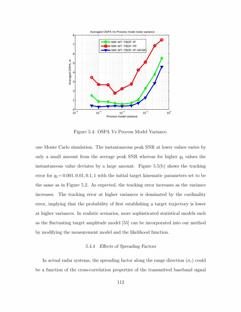
10−4

10−3

10−2

10−1

100

0

1

2

3

4

5

6

7

8

Process model variance

Ave

rage

d O

SP

A, m

Averaged OSPA Vs Process mode noise variance

MM−MT−TBDF−IPMM−MT−TBDF−PFMM−MT−TBDF−IP−MCMC

Figure 5.4: OSPA Vs Process Model Variance.

one Monte Carlo simulation. The instantaneous peak SNR at lower values varies by

only a small amount from the average peak SNR whereas for higher q2 values the

instantaneous value deviates by a large amount. Figure 5.5(b) shows the tracking

error for q2=0.001, 0.01, 0.1, 1 with the initial target kinematic parameters set to be

the same as in Figure 5.2. As expected, the tracking error increases as the variance

increases. The tracking error at higher variances is dominated by the cardinality

error, implying that the probability of first establishing a target trajectory is lower

at higher variances. In realistic scenarios, more sophisticated statistical models such

as the fluctuating target amplitude model [55] can be incorporated into our method

by modifying the measurement model and the likelihood function.

5.4.4 Effects of Spreading Factors

In actual radar systems, the spreading factor along the range direction (σr) could

be a function of the cross-correlation properties of the transmitted baseband signal

112

5 10 15 20 25−20

−10

0

10

20

Time Step, k

Pea

k S

NR

, dB

q2 = 0.001

q2 = 0.01

q2 = 0.1

q2 = 1

(a)

0 10 20 30 40 500

2

4

6

8

10

12

Time Step, k

OS

PA

(16,

2)

q2 = 0.001

q2 = 0.01

q2 = 0.1

q2 = 1

(b)

Figure 5.5: Effects of Intensity Modeling Error Variance: (a) Instantaneous Peak

SNR for Target 1; and (b) OSPA Versus Time for Various Values of q2.

whereas the spreading factor in the range-rate direction (σr) could be related to the

number of pulses used for coherent processing [45]. The spreading factor in the az-

imuthal direction (σθ) is controlled by the antenna beamwidth [47]. In this simulation,

we evaluate the performance of our algorithm for different values of spreading factors

in order to investigate the degree of difficulty in tracking a low observable targets

by radars with different system parameters. We compare the tracking performance

under four different cases (i) σr =0.509 m, σr =0.077 m/s, and σθ =0.033 rad, (ii)

σr =0.636 m, σr =0.096 m/s, and σθ =0.041 rad, (iii) σr =0.764 m, σr =0.116 m/s,

and σθ =0.049 rad, (iv) σr =0.891 m, σr =0.135 m/s, and σθ =0.058 rad. The “one

sigma” measure for all four cases corresponds to 1, 1.25, 1.5, 1.75, respectively, times

the bin resolution in each measurement axis. In this section and the following sec-

tions, we refer to these four cases as 1σ, 1.25σ, 1.5σ, and 1.75σ, respectively. Figure

5.6(a) and 5.6(b) show the tracking error and the target existence probability respec-

tively, for all four cases at 3 dB peak SNR averaged over 60 Monte Carlo simulations.

113

0 10 20 30 40 500

2

4

6

8

10

12

14

16

Time Step, k

OS

PA

(16,

2)

1.75σ 1.5σ 1.25σ 1σ

(a)

5 10 15 20 25 30 35 40 450

0.2

0.4

0.6

0.8

1

Time Step, k

Pro

babi

lity

1.75σ 1.5σ 1.25σ 1σ

(b)

Figure 5.6: Effects of Spreading Factors: (a) OSPA Versus Time for Various Spreading

Factors; and (b) Probability of Target Existence Computed Using Equation (4.29),

Red: Target 1, Blue: Target 2, Black: Target 3.

The tracking error is very small for the 1.75σ case and for 1.5σ case, the tracking

error is still small except during mode transitions. The increased error at these times

is due to the increased cardinality error. When the spreading factor is at 1.25σ, it

takes a long time to detect new targets that entered the FOV. This is seen from the

slow rise of the target existence probability. The localization error is reduced as more

measurements are processed. The tracking performance is severely affected for the

1σ case. This is due to that fact that as the number of bins occupied by the target

associated measurement is reduced, the discrimination between noise and target is

minimal. Despite the poor multi-target tracking performance, the algorithm is still

able to reasonably detect the presence of all three targets as seen from Figure 5.6(b).

The target existence probability for Target 1 from time steps 25 to 41 is high since,

Targets 2 and/or 3 are not being detected before Target 1 leaves the FOV. Hence,

Targets 2 or 3 are detected as Target 1 after correctly detecting the disappearance of

114

the original Target 1. Therefore, the OSPA is dominated by the cardinality error due

to this higher probability of missed targets. The mode probabilities estimated using

Equation (4.19) and averaged over all Monte Carlo runs are shown in Figure 5.7 for

the test cases (i) and (iii). The figure shows the probabilities corresponding to all

possible modes in Table 4.2. The proposed algorithm closely follows the true mode

transition and the mode probabilities decrease as the spreading factor is decreased.

5 10 15 20 25 30 35 40 450

0.2

0.4

0.6

0.8

1

1.2

Time Step, k

Pro

babi

lity

Pk,1

Pk,2 P

k,5 Pk,8 P

k,7P

k,4 Pk,1

Figure 5.7: Mode Probability Computed Using Equation (4.19) For Three Targets

Case, Solid: σr = 0.509, σr = 0.077, σθ = 0.033 (1σ), Dashed: σr = 0.764, σr =

0.116, σθ = 0.049 (1.5σ).

5.4.5 Peak SNR Analysis

Figure 5.8 compares the averaged OSPA (c=16, p=2, averaged across all time

steps from 30 Monte Carlo runs) for varying peak SNRs at four spreading factor cases.

When the spreading factors are at 1.75σ and 1.5σ, the error is also reasonable at lower

115

SNR values. The tracking performance at 1.25σ degrades for SNR less than 3 dB and

for 1σ case, the algorithm provides useful results only when the SNR is above 5 dB.

As we increase the SNR, the tracking error for all four cases converges to a lower

value. Since the tracking performance is sensitive to the spreading factors, one can

employ SNR dependent waveform agile signal processing to dynamically adjust the

transmitted waveform parameters to provide a trade-off between tracking error and

range/range-rate resolution [103], [104].

−4 −2 0 2 4 6 8 100

2

4

6

8

10

12

14

SNR, dB

Ave

rage

d O

SP

A, m

1.75σ1.5σ1.25σ1σ

Figure 5.8: Averaged OSPA Vs. Peak SNRs.

5.4.6 Closely Moving Targets Tracking Analysis

The tracking accuracy for three closely-moving targets is demonstrated next to

investigate the ability to resolve closely-moving targets. Two cases are considered: (i)

targets moving in the opposite direction and (ii) targets moving closely in the same

direction. In the first case, we investigate the ability to continually track targets that

come close to each other and proceed in the opposite direction. In the latter case, we

consider the case of resolving two closely-moving targets. The initial target states in

the first case are set to (2.2, 0.2) m and (0.3, 0.50) m/s, (12.2, 13.2) m and (-0.40,

116

2 3 4 5 6 7 8 9 10 11 120

2

4

6

8

10

12

14

16

Target 1 Start

Target 2 Start

Target 3 Start

x

y

(a)

0 2 4 6 8 10 12 14 16 180

2

4

6

8

10

12

14

16

18

Target 1 Start

Target 2 StartTarget 3 Start

x

y

(b)

Figure 5.9: Closely-Moving Targets Case: (a) Trajectory of Targets Moving in Op-

posite Direction; and (b) Trajectory of Targets Moving in Same Direction.

-0.45) m/s, and (9.2, 16.2) m and (-0.30, -0.70) m/s for Target 1, Target 2, and Target

3, respectively, and the targets enter and leave the FOV at time steps 5, 13, 21 and

25, 33, 41, respectively. In the second case, the initial kinematic states for Targets

1–3 are (3.4, 3.4) m and (0.4, 0.4) m/s, (1.9, 1.9) m and (0.475, 0.475) m/s, and (0.4,

0.4) m and (0.55, 0.55) m/s, respectively and the targets enter and leave the FOV at

time steps 4, 7, 10 and 33, 36, 39, respectively. Figure 5.10(a) shows the Euclidean

distance between target pairs for both test cases. Targets are within 1 m of each

other at time step 25 and 32 for case (i) and (ii), respectively. In the second case, the

Euclidean distance between targets in range-rate is around 0.1-0.2 m/s (≈ 1.5–3 times

the bin resolution) and the Euclidean distance between targets in the look direction

is around 0.01 degrees (less than one bin resolution). Figure 5.9(a) and Figure 5.9(b)

show the target trajectories for both test cases. Figure 5.10(b) shows the tracking

error averaged over 60 Monte Carlo runs at 3 dB peak SNR with the spreading factor

set to 1.5σ. The cardinality error is generally high around mode transitions than the

well separated targets case. The tracking error for case (ii) is high from time steps

117

5 10 15 20 25 30 350

1

2

3

4

5

6

7

8

9

10

11

Time,k

Dis

tanc

e, m

Target 1 & 2Target 1 & 3Target 2 & 3

(a)

0 10 20 30 40 500

1

2

3

4

5

6

7

8

9

10

Time Step, k

OS

PA

(16,

2)

Closely moving targets in opposite directionClosely moving targets in same direction

(b)

Figure 5.10: Closely-Moving Targets Case: (a) Euclidean Distance Between 3 Closely-

Moving Targets (Crosses Represent Targets Moving in Opposite Directions); and (b)

Tracking Error, OSPA(16, 2).

33–39 since the targets come close to each other before one of them leaves from the

FOV and the algorithm continues to track the non-existent target. This is because

the predicted measurement likelihood corresponding to this target is high due to the

presence of other targets in the neighbourhood of the predicted target state. For a

target that leaves the FOV with similar kinematic state estimates as another existing

target, the predicted state vector obtained using the state transition matrix is also

estimated in the vicinity of the already existing target. Hence, it takes longer to

detect the disappearance of closely-moving targets.

5.4.7 Six Targets Tracking Analysis

The algorithm performance for L =5 to track six closely-spaced targets at 3 dB

peak SNR with the spreading factor set at 1.5σ is demonstrated in Figures 5.11

and 5.12. The initial positions and velocities for Targets 1–6 are (2.2, 2.2) m and

(0.32, 0.32) m/s, (2.2, 0.2) m and (0.33,0.32) m/s, and (13.2, 15.2) m and (-0.14,

118

-0.32) m/s, and (13.2, 16.2) m and (-0.16, -0.34) m/s, and (10.1, 2.1) m and (-0.09,

0.09) m/s, and (11.1, 1.2) m and (-0.29, 0.14) m/s, respectively. Targets 1–6 enter

and leave the FOV at time steps 5 and 45, 11 and 51, 17 and 57, 23 and 63, and

29 and 69, and 50 and 65, respectively. The initial target states are selected such

0 5 10 150

2

4

6

8

10

12

14

16

x co−ordinate

y co

−or

dina

te

#1 Start

#2 Start#6 Start

#5 Start

#3 Start#4 Start

#1 End

#2 End

#3 End#4 End

#6 End

#5 End

Figure 5.11: Particle Distribution for Tracking Six Targets Case with L =5 Targets.

that there are two sets of closely-spaced targets with each set of targets moving in

opposite direction and the target pairs 1,3, 1,4, 2,3, 3,5, 4,5 and 4,6

cross each other at time steps 30, 34, 36, 50, 56 and 61, respectively. Figure 5.11

shows the higher likelihood particles corresponding to the marginal distribution of

each detected target. The starting and ending position of targets are indicated by

cross and star shaped markers, respectively. Target 6 entered the FOV after the first

119

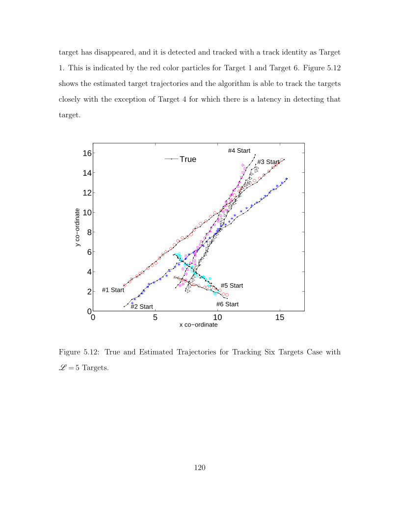
target has disappeared, and it is detected and tracked with a track identity as Target

1. This is indicated by the red color particles for Target 1 and Target 6. Figure 5.12

shows the estimated target trajectories and the algorithm is able to track the targets

closely with the exception of Target 4 for which there is a latency in detecting that

target.

0 5 10 150

2

4

6

8

10

12

14

16

#1 Start

x co−ordinate

y co

−or

dina

te

#2 Start

#3 Start

#4 Start

#5 Start

#6 Start

True

Figure 5.12: True and Estimated Trajectories for Tracking Six Targets Case with

L =5 Targets.

120

5.4.8 Performance Comparison Between PHDF-TBDF and

MM-MT-TBDF-IP-MCMC

In this section, we show the performance of the partitioning method for the 2-D

image measurement discussed in Section 4.5.1 to track three targets using the same set

of measurement parameters used by the authors in [67] and in Section 4.5.1. In [67],

the performance of PHDF-TBDF was compared using a single sensor and multiple

sensors and it was showed that the PHDF-TBDF needs measurements from at least

5 sensors for better tracking performance. In our simulation, we showed that we

can obtain better results even with a single sensor measurement with our proposed

algorithm. Figure 5.13 shows the tracking error (OSPA) with c = 40 and p = 2 at

19.8 dB, 16.3 dB, 13.8 dB peak SNR after averaging the OSPA from 100 Monte Carlo

simulations (same number of Monte Carlo simulations used in [67]).

0 5 10 15 20 250

0.5

1

1.5

2

2.5

3

Time, k

OS

PA

, m

OSPA(40,2) Vs SNR

SNR=19.8 dB,N = 250SNR=16.3 dB,N = 250SNR=13.8 dB,N = 250SNR=13.8 dB,N = 750

(a)

0 5 10 15 20 250

2

4

6

8

10

12

14

Time, k

OS

PA

, m

OSPA(40,2) Vs SNR

SNR=10.2 dB,N = 750

(b)

Figure 5.13: Image Measurement Case: (a) OSPA at Different Peak SNR (19.8 dB,

16.3 dB, 13.8 dB); and (b) OSPA at 10.2 dB Peak SNR.

The tracking error is small at 19.8 dB and 16.3 dB even when using a smaller

number of particles. The cardinality error is very small, indicating that the algorithm

correctly tracks the number of existing targets without any false detection. The

121

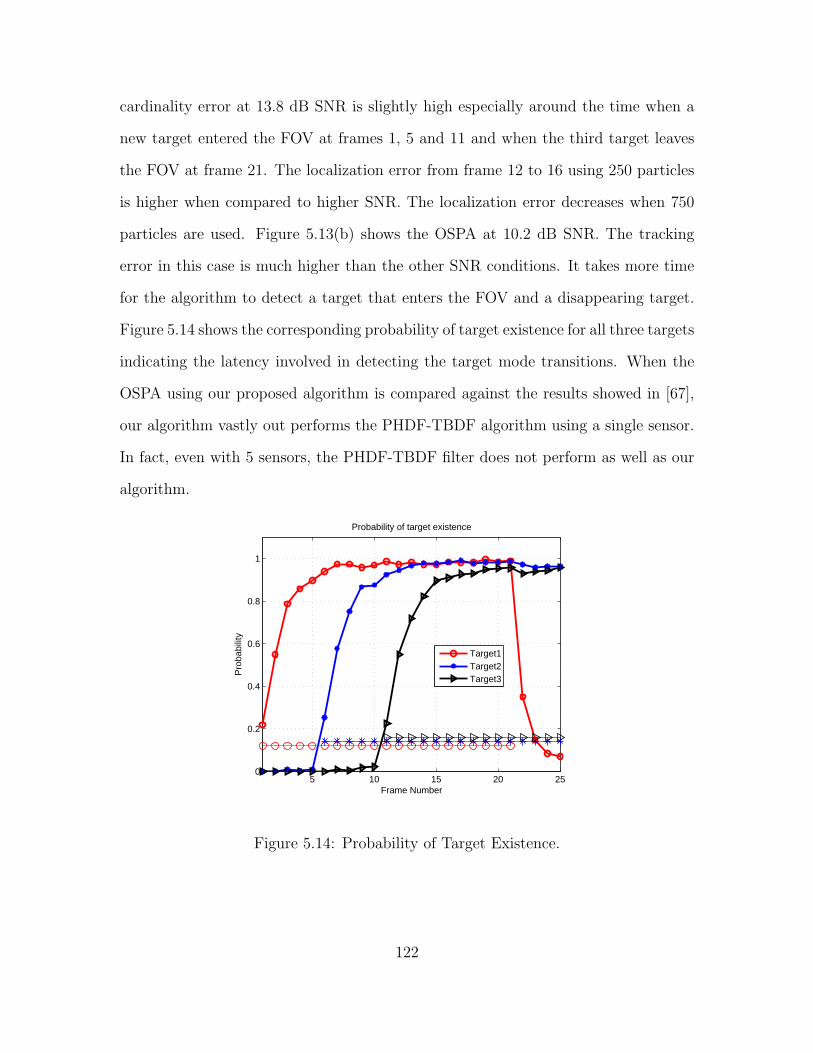
cardinality error at 13.8 dB SNR is slightly high especially around the time when a

new target entered the FOV at frames 1, 5 and 11 and when the third target leaves

the FOV at frame 21. The localization error from frame 12 to 16 using 250 particles

is higher when compared to higher SNR. The localization error decreases when 750

particles are used. Figure 5.13(b) shows the OSPA at 10.2 dB SNR. The tracking

error in this case is much higher than the other SNR conditions. It takes more time

for the algorithm to detect a target that enters the FOV and a disappearing target.

Figure 5.14 shows the corresponding probability of target existence for all three targets

indicating the latency involved in detecting the target mode transitions. When the

OSPA using our proposed algorithm is compared against the results showed in [67],

our algorithm vastly out performs the PHDF-TBDF algorithm using a single sensor.

In fact, even with 5 sensors, the PHDF-TBDF filter does not perform as well as our

algorithm.

5 10 15 20 250

0.2

0.4

0.6

0.8

1

Frame Number

Pro

babi

lity

Probability of target existence

Target1Target2Target3

Figure 5.14: Probability of Target Existence.

122

5.5 Computational Complexity Analysis

5.5.1 Heuristic Decision-directed Approaches

One of the drawbacks of our proposed method is that the number of modes in-

creases exponentially as a function of the maximum number of targets. The IP step

greatly reduces the required number of particles. However, some of the computa-

tional gains achieved by the IP is offset by the increase in computations required

by the MCMC. We thus demonstrate how to greatly reduce the combinatorial com-

plexity of the proposed algorithm using two decision-directed practices based on the

estimated mode and target existence probabilities.

0 10 20 30 40 500

5

10

15

20

25

30

Frame number, k

proc

essi

ng ti

me,

sec

Average processing time

All modesOpt (Th=0.001)Opt (Th=0.01)Opt (Th=0.1)

(a)

0 10 20 30 40 500

0.1

0.2

0.3

0.4

0.5

0.6

0.7

0.8

k

OS

PA

(16,

2)

OSPA, c = 16, p = 2

All modesOpt (Th=0.001)Opt (Th=0.01)Opt (Th=0.1)

(b)

Figure 5.15: Computational Analysis: (a) Processing Time Difference Between all

Modes and Mode Probability Selected Modes; and (b) OSPA Difference Between all

Modes and Mode Probability Selected Modes.

For the first practice, if the estimated number of existing targets is less than the

assumed maximum number of targets, then there is no need to propagate particles

corresponding to all the modes. For example, if at time step k, there is only one

target in the FOV, then the computations to propagate the PF to modes that tran-

123

sition from three targets present are not necessary. In order to determine which PF

mode propagations are needed, we can compare the mode probability at the pre-

vious time step k−1 to a threshold. Specifically, if the probability corresponding

to mode j at time k−1 is very small, then at time k, the PF steps correspond-

ing to p(x[i]k |mk−1= j,mk = i,Zk) for all i at time k are not computed. Similarly,

if the mode probability for mode i at time k is small, then the PF corresponding

to p(x[i]k |mk = i,Zk) is not executed at time k. When this practice is followed, the

number of particles needed to approximate the posterior PDF of the ℓth target in

Equation (4.28) and the mode conditioned joint PDF in Equation (4.27) is much

smaller as the particles corresponding to low probability modes are ignored. For the

second practice, if the target existence probability at time k−1 is very small, then

it is not necessary to propagate the continuing particles. As a result, during the

implementation of the first layer of PFs, we propagate the continuing particles and

corresponding partitions only if the target existence probability estimate at the pre-

vious time step is greater than some threshold. As the number of selected modes is

dependent on the probability threshold, the processing time also varies as a function

of the threshold. In our simulations, we compare the processing time using 0.1%, 1%,

and 10% thresholds. Figure 5.15(a) shows the time required to process one time step

of data in Matlab using a 2.5 GHz Intel i5 core processor with and without the two

aforementioned practices; the simulation is for tracking L =3 targets at 3 dB peak

SNR using 1,000 particles. The initial target parameters used to generate Figure

5.15(a) is used for this analysis. The peak processing time (PPT) is reached when

all targets are present. Our simulations showed that when all modes are selected, the

PPT is 28 s; 7 s are needed when only the high probability modes are selected. The

PPT increases only slightly when the thresholds are reduced. The number of modes

with significant mode probability is usually higher during mode transitions. Hence,

124

1 1.5 2 2.5 3 3.5 4 4.5 5−50

0

50

100

150

200

250

Maximum number of targets

Pro

cess

ing

time

, sec

Avg (all modes)Avg (opt.)Peak (all modes)Peak (opt.)Avg(opt. linear approx)Peak(opt. linear approx)

Figure 5.16: Average and Peak Processing Time for Different Maximum Number of

Targets.

the processing time is higher around the mode transitions at lower thresholds. Figure

5.15(b) shows the OSPA comparing the different test cases. Although the tracking

error is similar for all test cases, the best tracking performance was obtained with

a 10% threshold. The increased tracking error for the other cases resulted from the

increased cardinality error during mode transitions. This could be due to the noisy

measurements preventing occasional false detections of target existence when a higher

threshold is used. Overall, the computational cost is reduced with no significant loss in

tracking performance when the low probability modes are ignored. Figure 5.16 shows

the average and PPT per time step for different maximum number of targets L . As

shown, the average and PPT increase almost linearly instead of exponentially as a

function of the maximum number of targets, when the practices are applied. Using

linear regression, the average and PPT for 1,000 particles with a 10% threshold can

be linearly approximated by (1.803L − 1.447) s and (5.11L − 6.765) s, respectively.

125

5.5.2 Effects of Particle Filter Size

Figure 5.17 shows the performance improvement that can be achieved by increas-

ing the number of particles (Nj,i, Ni and Nℓ) at 3 dB and -3 dB peak SNR for the

three targets case in Figure 5.17(a). The averaged OSPA reaches a steady state error

for the 3 dB case at 1,000 particles, and for the -3 dB case, it reaches the steady

state error at around 2,500 particles. It requires more number of particles at -3 dB

SNR to achieve a similar tracking error as in the 3 dB case. Figure 5.17(b) shows the

corresponding average and PPT per time step for different number of particles and

the processing time is similar under both SNR conditions.

0 500 1000 1500 2000 2500 3000 3500 40000

0.2

0.4

0.6

0.8

1

1.2

1.4

1.6

1.8

Number of particles

Ave

rage

d O

SP

A, m

3 dB SNR−3 dB SNR

(a)

0 500 1000 1500 2000 2500 3000 3500 40000

10

20

30

40

50

60

70P

roce

ssin

g tim

e, s

ec

Number of particles

Average (3 dB SNR)Peak (3 dB SNR)Peak (−3 dB SNR)Average (−3 dB SNR)

(b)

Figure 5.17: Effects of Partilce Filter Size for L = 3 Targets: (a) Tracking Error;

and (b) Average and Peak Processing Time.

126

Chapter 6

TRACK-BEFORE-DETECT FILTERING OF MULTIPLE TARGETS IN SEA

CLUTTER

6.1 Target Tracking in Sea Clutter

Target detection and tracking in clutter is a challenging problem, especially when

the reflected signal characteristics from clutter are similar to target associated signals.

In moving target indicator applications, clutter effects can be mitigated using coher-

ent processing by separating the moving target from stationary clutter objects using

simple filtering steps in the frequency domain [45]. However, in sea based radars, the

radial velocity of clutter is usually high due to the presence of moving waves on the

sea surface. The radial velocity of these waves can be significant depending on the

sea state that is influenced by various weather and wind conditions [89]. The spiky

nature of sea clutter further complicates the target detection and tracking problem.

These target like outliers can increase false target detections which in turn affects

the computational complexity of conventional detect-before-track algorithms due to

combinatorial processing. Hence, accurate modeling of the sea clutter random process

is critical for improved tracking performance. The compound Gaussian model [89]

is a well established statistical model to characterize the reflected signal associated

with sea clutter. The tracking problem becomes more complicated when the radar

cross section (RCS) of the target to be tracked is very small. For example, in mar-

itime surveillance applications, it is of critical importance to detect and track a small

enemy boat [108]. It was shown in [109] that the signal-to-clutter ratio (SCR) can be

improved using real sea clutter by performing principal component analysis (PCA)

127

on the received data and selecting only the principal components that correspond

to a few of the lowest singular values. The main assumption in this method is that

the clutter level is usually much higher than the target associated signal and that

by selecting only the minor components, the target associated components are sepa-

rated from the clutter. Using this approach, a subspace based sea clutter suppression

method was proposed in [110] that improves the detection performance. Despite using

accurate statistical models and various signal enhancement techniques, conventional

detect-before-track methods still suffer from heavy clutter and low RCS. The tracking

problem becomes even more difficult if there is a need to track multiple low observable

sea targets. The SMC based track-before-detect filter (TBDF) algorithm for tracking

low observable targets can be an attractive alternative as it can be combined with

particle filtering (PF) methods [17].

Estimating the clutter statistics from raw measurement is one way to improve

the detection and tracking of targets in clutter environments. Since the clutter as-

sociated returns evolve over time, the clutter information must be estimated directly

from the measurements [111]. Most of the methods rely on estimating the clutter

statistics from the neighbourhood bins of a range-Doppler bin under consideration.

Three well-known clutter estimation methods relating to a constant false alarm rate

(CFAR) were compared in [112]: cell averaging, cell averaging greatest of, and order

statistics. It was shown that the OS method is more susceptible to the effects of spiky

sea clutter whereas the CA method is the most robust among the three methods. In

[113], the clutter point spatial density in non-homogeneous clutter background was

estimated using maximum likelihood (ML) and approximated Bayesian methods. The

intensity function of this non-homogeneous Poisson point process was approximated

by a Gaussian mixture model and then integrated into the probability hypothesis

density filter (PHDF). Moreover, the clutter spatial density was estimated over the

128

entire field of view (FOV) and the tracker output was used to enhance the estimate

of clutter spatial density. A PF based ML method was used to estimate the clutter

parameters [114, 115]. In [116, 117], any non-homogeneous clutter spatial density was

modeled as a Gaussian mixture. The approximated Bayesian estimate of the inten-

sity function was updated iteratively using the normal-Wishart mixture PHDF. This

clutter intensity function estimate was integrated with joint integrated probabilistic

data association or multiple hypothesis testing algorithms to track multiple targets.

In this method, the clutter spatial density estimation problem was converted into a

clutter generator estimation problem solved using the PHDF. The likelihood func-

tion of the clutter generator was assumed to be Gaussian with unknown mean and

covariance, and the clutter generator PHDF was derived using a mixture of normal-

Wishart probability density function (PDF). A closed form expression for the clutter

generator PHDF was also derived.

A recursive TBDF was proposed in [118] for estimating clutter statistics as a part

of the likelihood evaluation step. Specifically, the clutter level was estimated by av-

eraging over a set of nearby bins not affected by a target. Guard bins around the

target state were used to estimate the clutter variance, and a grid based numerical

evaluation was used to compute the likelihood ratio for Rayleigh distributed clutter.

A multi-scale adaptive single target TBDF method using the beamlet transform was

proposed in [119] for maritime environments. In this method, the longest chained

beamlet path whose length was greater than a threshold was detected as a potential

target. In [120], a Viterbi-like multi scan TBDF algorithm was proposed in complex

Gaussian clutter using space-time processing and the algorithm’s detection perfor-

mance was analyzed.

Very few multiple target TBDF methods in spiky sea clutter environments have

been considered thus far in the literature. In this chapter, we extend our proposed

129

multiple mode multiple target TBDF (MM-MT-TBDF) algorithm [76, 81] for complex

Gaussian (low resolution radar) and compound Gaussian (high resolution, low grazing

radar) sea clutter using pulse Doppler radar measurements. The likelihood functions

needed for the TBDF approach can be computed using classical techniques, thereby

exploiting some of the optimal methods that have already been derived through rigor-

ous mathematical steps. For the compound Gaussian model, the texture component

is assumed to follow a known distribution function [121, 122]. In this case, the optimal

generalized likelihood function is not mathematically tractable. Hence, various sub-

optimal but asymptotic detectors have been proposed in the literature [85, 123, 124].

In [110], instead of a known a priori distribution assumption, the texture compo-

nent is assumed to be deterministic. Based on this assumption, we derive an optimal

likelihood function and the ML estimation of the texture component and the speckle

covariance matrix which can be implemented using a fixed point algorithm [83, 84].

We also investigate the relationship between this optimal and the sub-optimal likeli-

hood function in [85].

6.2 Measurement from Pulse Doppler Radar with Clutter

A pulse Doppler radar transmits a series of pulses with a pulse repetition interval

TPRI. To increase the radar range resolution, these pulses are modulated by higher

bandwidth (fs) signals such as frequency modulated chirps [45]. The modulated base-

band signal is further modulated by the carrier frequency fc before emitting from the

transmitting antenna. The transmitted signal is reflected by many scatterers that are

present in the FOV of the radar. The received complex baseband signal after carrier

demodulation is typically sampled at the frequency equal to the bandwidth (fs) of

the baseband modulating signal and these samples are referred as fast time samples.

The Doppler processing is performed through spectral analysis of the samples ob-

130

tained by sampling the received signal at the rate of 1/TPRI. The samples used for

the spectral analysis are referred as slow time samples. The period during which the

measurements from a set of pulses used for Doppler analysis is referred as dwell.

We consider measurements from a pulse Doppler radar that is operating at a pulse

repetition interval TPRI and transmitting Np pulses per dwell in the presence of fast-

varying clutter. Each dwell is assumed to transmit the same pulse s[n] = s[n/fs],

n = 0, 1, . . . Ns−1 whereNs is the number of samples and fs is the sampling frequency.

The received signal consists of reflections from multiple targets from all the dwell

pulses, in addition to clutter due to multiple undesirable reflections from scatterers.

It is assumed that the number of scatterers and their Doppler frequency remain the

same during the transmission of all Np pulses in the same dwell. Assuming that

measurements are received from a preset direction of arrival (DOA), an (Nv × Np)

measurement matrix corresponding to the received signal from all Np pulses at the

kth dwell can be written as

Yk = S(Tk +Ak) +Wk (6.1)

where Wk is the (Nv ×Np) uncorrelated measurement noise matrix, and Nv = ζNv −

ζ1+1 is the number of range bins in the validation gate (i.e., the region of measurement

selection for track updates) where ζi is the ith range bin in the validation gate. In this

linear model, the overall clutter scatterer contribution at the kth dwell is generalized

by the (Nr ×Np) reflectivity matrix Ak as

Ak =

ak[ζ1, 0] ak[ζ1, 1] . . . ak[ζ1, Np − 1]

ak[ζ2, 0] ak[ζ2, 1] . . . ak[ζ2, Np − 1]

......

......

ak[ζNr , 0] ak[ζNr , 1] . . . ak[ζNr , Np − 1]

(6.2)

131

where Nr =Nv+Ns−1, and the matrix elements ak[ζi, p], containing both reflectivity

and Doppler shift are defined as

ak[ζi, p] = ξk[ζi, p]ej2πνζipTPRI . (6.3)

where ξk[ζi, p] is the clutter reflectivity, νζi is the Doppler shift at range bin ζi, and

p = 0, 1, . . . Np − 1. Similarly, the reflectivity matrix Tk for multiple targets can be

written as a sparse matrix with non-zero complex reflectivity value in those range bins

where a point target is present at the kth dwell. The range bin number corresponding

to the range of the ℓth target at the kth dwell is represented as ζk,ℓ, where we also

include the dwell index k to indicate that the range bin corresponding to the ℓth

target varies with time. The range of the ℓth target and the corresponding range bin

ζk,ℓ are related as [45, 47]

ζk,ℓ = round

(2rk,ℓc

fs

)(6.4)

where c is the velocity of propagation, and rk,ℓ is the range of the ℓth target. The

target reflectivity and the Doppler shift for the ℓth target is represented as Ik,ℓ and

νk,ℓ, respectively, where we assume that the target reflectivity is constant across all

Np pulses. As in Equation (7.2), the range-rate information of a target is absorbed

in the complex reflectivity. The reflected signal from a target is modulated across Np

pulses by a slowly varying signal with the Doppler frequency νk,ℓ. Under narrowband

conditions, the Doppler frequency and the target range-rate rk,ℓ are related as [45, 47],

νk,ℓ =2rk,ℓc

fc (6.5)

where fc Hz is the carrier frequency. A circulant (Nv × Nr) signal matrix S is con-

132

structed from the transmitted signal s[n] as

S =

s[Ns − 1] 0 . . . s[0] 0 . . . 0 0

0 s[Ns − 1] . . . s[1] s[0] 0 . . . 0

......

......

......

......

0 0 . . . 0 s[Ns − 1] . . . s[1] s[0]

. (6.6)

Here we assume that the same baseband signal s[n] is used to transmit at all dwell

instances. The measurements at the kth dwell are vectorized to form the (NvNp × 1)

vector

zk = vec(Yk)

where vec(Yk) forms the (NvNp × 1) vector formed by concatenating the columns of

Yk and Zk = z1, z2, . . . , zk represents all the measurements up to dwell k.

In order to consider the contribution of the ℓth target present in the range bin

ζk,ℓ, the measurement vector extracted from the ζk,ℓth row vector of Yk in Equation

(6.1) can be written as

zk[ζk,ℓ] =

Li∑j=1

bj,ℓs[νk,j] + cTk[ζk,ℓ] (6.7)

where ck[ζk,ℓ] is the clutter measurement vector corresponding to the ζk,ℓth row of

matrix SAk in Equation (6.1). In order to jointly detect the existence of closely

spaced multiple targets, the reflectivity contribution from all targets to the range

bin ζk,ℓ should be considered. Here we assume that Li targets are present in the

preset DOA. The summation term in the model in Equation (6.7) represents the

signal level contribution to the range bin ζk,ℓ from all targets that are present in the

neighbouring range bins, and it is the vector corresponding to the ζk,ℓth row of matrix

133

STk in Equation (6.1). The scale factor bj,ℓ is the reflectivity contribution of the jth

target to the range bin ζk,ℓ, j=1, . . .Li. The reflectivity contribution bj,ℓ from the jth

target is a function of its reflectivity Ik,j, and it depends on the correlation properties

of the signal s[n]. Specifically, the contribution from the ℓth target to the range bin

ζk,ℓ is bℓ,ℓ = Ik,ℓ, and if the jth target is far away from the ℓth target, then bj,ℓ = 0.

The Doppler frequency corresponding to all targets are denoted as νk,j and

s[νk,j] = [1 e−j2πνk,jTPRI . . . e−j2πνk,j(Np−1)TPRI ]T.

Equation (6.7) can be written in matrix form as

zk[ζk,ℓ] = Sℓbℓ + ck,l[ζk,ℓ], (6.8)

where Sℓ is the (Np × Li) matrix

Sℓ =

[s[νk,1] . . . s[νk,Li

]

]and the (Li × 1) vector bℓ is given by

bℓ =

[b1,ℓ . . . bLi,ℓ

]T.

6.3 Compound Gaussian Clutter Model

6.3.1 Factors Affecting Statistical Sea Clutter Modeling

Different statistical models for clutter have been considered based on analyzing

data from real-life radar measurements. For example, in a typical data association

based target tracking application, the number of clutters that are being detected

inside the validation gate are usually assumed to be Poisson distributed [20]. The

clutter density is often assumed to be known a priori. If no a priori information is

available regarding the spatial density of the clutter, then it is commonly assumed to

134

be uniformly distributed in the FOV. In target detection problems, the clutter model

parameters of a selected probability density function [99], [125–128] are implicitly

estimated from measurements [129] and then used in the generalized likelihood ratio

test (GLRT) [46]. Based on this GLRT, a CFAR detector can be designed [45, 47,

130]. The detector performance is usually very sensitive to the type of statistical

clutter model selected for a particular application and therefore new techniques are

being developed to examine the validity of the chosen model using real-life clutter

measurements [131].

The backscatter signal level in a radar application can vary substantially based

on the grazing angle, thus directly affecting the underlying statistical model for the

received backscatter. For example, the backscatter level from sea clutter at higher

grazing angles is very high when compared to the level at lower grazing angles. The

clutter level difference between high and low grazing angles can vary by many tens

of dB. The backscattering in a low grazing angle radar is influenced by multiple path

reflections around the crests of sea waves. The multiple path reflections together with

the shadowing of wave trough can result in constructive and destructive cancellation

[47]. Different long tailed distributions have been suggested [89, 126–128, 132, 133]

to model this random phenomenon for a low grazing angle radar. Subsequent experi-

mental studies have found real data to be consistent with many of these distributions

[100, 134–138].

Another factor that affects the clutter statistics is the radar resolution. In a

low resolution radar, the cross sectional area corresponding to a single range bin is

high. The backscattered signal is a result of multiple reflections from many physical

objects that are present in this large area. The reflected signal from a large number

of such independent and randomly located scatterers is usually modeled as complex

Gaussian. The corresponding distributions in magnitude and magnitude squared form

135

are Rayleigh and exponential distributions, respectively. For low-resolution radars,

complex Gaussian is an appropriate approximations since the combined reflections

from many independent clutters in a low resolution range bin can be approximated

by the complex Gaussian distribution following the central limit theorem [92]. In high

resolution radars, the cross section area of a range bin under illumination is small,

therefore, the backscatter signals will exhibit spiky structures which can no longer

be approximated by complex Gaussian. This behaviour is more prominent in sea

clutters in which reflections from gravity waves and sea swells [89] can give rise to

spiky reflected signals that can be modeled using long tailed distributions. In [139]

many of the long tailed distributions were shown to provide a good fit to real data

from a high resolution radar in the Ka-band and in a sea clutter environment.

In this section, we use the complex Gaussian clutter model for a low resolution

radar and the compound Gaussian sea clutter model for a high resolution, low graz-

ing angle radar. These clutter models are incorporated into our MM-MT-TBDF

algorithm and the tracking performance under different SCR values is analyzed.

6.3.2 Speckle and Texture Sea Clutter Components

Clutter from a high resolution, low grazing angle radar has been characterized

by various long tailed probabilistic models such as compound Gaussian [140], K-

distribution [89, 128, 133], compound K-distribution [141], log-normal [126], Weibull

[127, 142], non central gamma distribution [143], chi-square [130], and generalized

compound [144] distributions. Recently, the Pareto distribution has also been pro-

posed for a high resolution radar with both high [145], [146] and low grazing angles

[147]. In our work, we adopted the compound Gaussian distribution to model sea

clutter, and using some simple and reasonable assumptions, we present a framework

for MM-MT-TBDF in sea clutter.

136

In the compound Gaussian model, clutter from sea surface is characterized by

two components, namely speckle and texture. The speckle component is due to

rapidly fluctuating, small scale structures with smaller decorrelation time, and it is

modeled using a complex Gaussian distribution. The speckle component is due to the

presence of multiple scatterers and it decorrelates through the relative motion of the

small structures. Recently, the validity of the complex Gaussian assumption for the

speckle component was corroborated using real radar data from the Ka-band, even

for range resolution in the order of few centimeters [139]. The texture component is

a slowly varying large scale structure that modulates the speckle component. The

texture component has a longer correlation time, and it is associated with the long sea

waves and swell structure. The texture component is usually modeled using either

the gamma distribution [89] or inverse gamma distribution [121]. Using these two

components, clutter at the kth dwell can be modeled using the compound Gaussian

model as

ck[ζi, p] =√

τk[ζi, p]k uk[ζi, p]

where τk[ζi, p] ≥ 0 represents the texture component that modulates the speckle

component u[ζi, p] corresponding to the pth pulse at range bin ζi. When the texture

is modeled as a gamma distribution, then the compound Gaussian model is the well

known K-distribution. The clutter from all pulses in the kth dwell is represented as

ck[ζi] =

[√τk[ζi, 0]uk[ζi, 0], . . . . . .

√τk[ζi, Np − 1]uk[ζi, Np − 1]

]T.

In general, the texture component within a dwell is also assumed to be randomly

distributed. However, if we choose the dwell duration to be very small, we could

assume that the texture component is the same for all pulses in a dwell [110]. This

is a reasonable assumption due to the slow varying nature of the texture component.

137

During this very short dwell duration, the delays corresponding to the scatterers and

their Doppler shifts in the signal model in Equation (6.1) are assumed constant. The

clutter vector can now be written as

ck[ζi] =√τk[ζi] [uk[ζi, 0] uk[ζi, 1] . . . uk[ζi, Np − 1]]T . (6.9)

The speckle component is assumed to vary from pulse to pulse since minor perturba-

tions in the same scale sea structures can change the overall effect of multiple path

reflections. The clutter covariance matrix is given by τk[ζi]Σ, whereΣ is the (Np×Np)

complex covariance matrix of the speckle component that is assumed to be the same

for all range bins. Since the dwell duration is assumed small, the speckle decorrelation

time is greater than the pulse interval duration and therefore, the speckle covariance

matrix is assumed to be a non-identity matrix.

6.3.3 Doppler Model for Sea Clutter

The sea surface consists of many complex but significant structures. The small

ripples on the sea surface are generated by blowing winds and these transfer the

energy to longer waves. When the wind is blowing at a constant speed, then these

sea waves reach an equilibrium condition [89] and are modulated by sea swells from

neighborhood regions that are stimulated by turbulent weather conditions. Clutter

from local wind driven ripples is usually modeled as Bragg’s scattering [47]. The

radial velocity of these ripple waves is usually low. The radial velocity associated

with the modulating sea swells is usually higher than that of the Bragg’s scattering.

Many empirical studies have shown that the averaged Doppler spectrum of sea clutter

can be modeled by a combination of fast non-Bragg scattering associated with the

sea swells and a slow Bragg’s scattering that is associated with the smaller capillary

waves [138, 148, 149]. The relation between the mean value of the backscatter signal

138

and the mean Doppler shift were investigated in [88, 150]. A linear approximation

model that relates the texture component and the Doppler frequency was used in

[87] to model the Doppler spectra. We used this model to generate complex clutter

measurements with Doppler information as follows.

• We randomly generate a Doppler frequency corresponding to Bragg’s scattering

that is assumed to have a Gaussian distribution whose mean µBragg corresponds

to a lower frequency and its variance σ2Bragg is set to a fixed pre-determined

value.

• We generate the Doppler frequency corresponding to sea swell by randomly sam-

pling from a Gaussian distribution whose mean frequency µswellk [ζi] = Aswell +

Bswellτk[ζi] is linearly related to the texture component value, where Aswell and

Bswell are model parameters. The variance of the Gaussian distribution σ2swell

is selected from another Gaussian distribution with preset mean and variance

[87, 88].

• The Doppler frequency corresponding to a dwell in Equation (7.2) is randomly

selected between a Bragg’s scattering frequency or a swell frequency such that

the averaged Doppler spectra over a large number of dwells consists of two main

Doppler components similar to the one fitted from real data in [138, 148, 149].

6.4 Likelihood Function in Complex Gaussian Clutter

In most radars operating in a heavily cluttered environment, the clutter strength

is much higher than that of the measurement noise. Thus, for simplicity, we use the

likelihood function derived assuming that only clutter is present. A similar derivation

can be extended to include noise following the principles mentioned in [125, 151]. The

target presence condition in a range bin can be formulated as a binary hypothesis

139

problem. From Equation (6.8), we consider the measurement zk[ζk,ℓ] corresponding

to range bin ζk,ℓ from all Np pulses in dwell k. Using this measurement, the two

hypothesis are given by

H0 : zk[ζk,ℓ] = cTk[ζk,ℓ]

H1 : zk[ζk,ℓ] = Sℓbℓ + cTk[ζk,ℓ]. (6.10)

Without loss of generality, we replace the measurement vector zk[ζk,ℓ] with zk,ℓ to

simplify notation. In this section, we explain only about the likelihood function in

mode i and recall Li is the number of targets in mode i. Based on the binary

hypothesis model in Equation (6.10) and the complex Gaussian assumption, we can

write the generalized likelihood ratio for a range bin corresponding to the state vector

x[i]k,ℓ in mode i as [152]

L(zk|x[i]k,ℓ) = L0/L1, (6.11)

where

L0 = NT + zHk,ℓΣ−1zk,ℓ ,

L1 = NT + (zk,ℓ − Sℓbℓ)HΣ−1(zk,ℓ − Sℓbℓ) .

Here, H represents conjugate transpose, Σ is the ML sample covariance estimate of the

complex covariance matrix of the clutter statistics that is obtained using NT > Np

secondary range bins [152]. Specifically, the sample covariance matrix estimate is

given by

Σ =1

NT

NT∑n=1

zk[n]zk[n]H. (6.12)

where zk[1], . . . , zk[NT ] are the secondary range bins in the vicinity of the range bin

under testing. The likelihood ratio in (6.11) depends on the reflectivity of multiple

140

targets. The explicit estimation of the target reflectivity can be avoided by substitut-

ing the analytical solution of bℓ that maximizes the likelihood function in (6.11). The

likelihood function is maximized when the quadratic quantity in L1 is minimized. For

a positive definite matrix Σ, the weighted least squares solution of bℓ that minimizes

the quadratic term is given by

b(LS)ℓ = (SH

ℓΣ−1Sℓ)

−1(SHℓΣ

−1zk,ℓ).

Substituting b(LS)ℓ in L1 we obtain

L1 = NT + zHk,ℓΣ−1zk,ℓ − (zHk,ℓΣ

−1Sℓ)b(LS)ℓ .

Upon further simplification, the generalized likelihood function can now be derived

as

L(zk|x[i]k,ℓ) =

1

1− ηG(zk|x[i]k,ℓ)

,

where

ηG(zk|x[i]k,ℓ) =

(zk,ℓΣ−1SH

ℓ)(SHℓΣ

−1Sℓ)−1(SH

ℓΣ−1zk,ℓ)

(NT + zHk,ℓΣ−1zk,ℓ)

. (6.13)

Thus, the contribution of targets present in the neighbourhood range bins are also

considered in the generalized likelihood function derivation. The likelihood value

tends to infinity if a target exists in the selected range bin; otherwise it tends to zero

[152]. Since we use the generalized likelihood function, there is no need to estimate

the signal intensities Ik,ℓ. The dimension of the matrix Sℓ in mode i depends on the

number of assumed targets in that mode, and the predicted Doppler frequencies of

the corresponding targets are used to construct the columns of this matrix. If the

targets are moving farther apart such that the reflected signals from other targets do

not contribute to the range bin corresponding to the ℓth target, i.e., Sℓ = s[νk,ℓ], then

the test statistic can be further simplified as

ηG(zk|x[i]k,ℓ) =

∣∣s[νk,ℓ]HΣ−1zk,ℓ∣∣2

s[νk,ℓ]H Σ−1 s[νk,ℓ][NT + zHk,ℓ Σ

−1 zk,ℓ] . (6.14)

141

This simplified likelihood function is the same expression derived in [152] for detecting

a single target.

6.5 Likelihood Function in Compound Gaussian Clutter

In the compound Gaussian case, the binary hypothesis problem in Equation (6.10)

is still valid. The additive clutter is assumed to be complex compound Gaussian

distributed, and the derivation of the generalized likelihood function is more involved

than that of the complex Gaussian case, leading to different detector forms [121, 123,

124, 153–155]. As the clutter covariance matrix is a critical parameter in a GLRT

detector, the covariance matrix of compound Gaussian clutter is a research topic

under investigation [122, 156–159].

6.5.1 Asymptotic Generalized Likelihood Function

An asymptotically optimum GLRT detector that is independent of the texture

PDF was proposed in [124]. The test statistics using this detector for well separated

targets can be written as

ηLQ(zk|x[i]k,ℓ) =

∣∣∣∣s[νk,ℓ]HM−1zk,ℓ

∣∣∣∣2(s[νk,ℓ]HM−1s[νk,ℓ]

)(zHk,ℓM

−1zk,ℓ

) (6.15)

where M is the clutter covariance matrix in the range bin under test. Note that, in

the compound Gaussian model, the clutter power between range bins is not assumed

the same, hence the clutter covariance matrix is different between different range

bins. This detector is derived based on the linear-quadratic (LQ) detector originally

derived for a compound Gaussian clutter with the assumption that the covariance

matrix M is known [85, 86]. This detector is referred to as normalized matched filter

(NMF). When we assume that the texture component is constant across the entire

142

dwell, then the test statistic only depends on the structure of the speckle covariance

matrix and can then be written as


∣∣∣∣s[νk,ℓ]HΣ−1zk,ℓ

∣∣∣∣2(s[νk,ℓ]HΣ−1s[νk,ℓ]

)(zHk,ℓΣ

−1zk,ℓ

) (6.16)

Recall that we assume that the speckle covariance matrix structure is the same for all

range bins. When the covariance matrix Σ is substituted by its estimate, the detector

is called M-adaptive NMF (M-ANMF) or Σ-adaptive NMF (Σ-ANMF) depending on

the covariance matrix estimation method [123, 156]. The M-ANMF sample covariance

estimate is given by

ΣM =1

NT

NT∑n=1

zk[n]zk[n]H (6.17)

and the Σ-ANMF sample covariance estimate based on the normalized secondary

range bins is given by

ΣΣ =1

NT

NT∑n=1

zk[n]zk[n]H

1Np

zk[n]Hzk[n](6.18)

where NT is the number of secondary range bins. A different estimator for Σ was

proposed in [156] under the assumption that the clutter power spectral density is

symmetric about the zero Doppler frequency. However, this assumption does not

generally hold for the averaged Doppler spectrum of real sea clutter as it exhibits

an asymmetric pattern around the peak Doppler frequency [89, 138]. In [123], the

detector in Equation (6.15) was reformulated by replacing the covariance matrix with

its eigen decomposition. The covariance matrix is assumed to be circulant so that the

basis function of the discrete Fourier transform (DFT) can be used as the eigenvec-

tors [160]. The normalized sample mean of the DFT coefficients of the measurement

vectors from the primary and secondary range bins are approximated as the eigenval-

ues. In computer simulations, this detector has been shown to perform better than

143

the M-ANMF and Σ-ANMF detectors. However, the circulant matrix assumption is

reasonable only when a large number of pulses are used for coherent processing.

6.5.2 Adaptive Generalized Likelihood Function Based on Kelly’s Method

In this section, we derive a multiple target generalized likelihood function for

compound Gaussian clutter by following Kelly’s approach [152]. For the binary hy-

pothesis problem in Equation (6.10), we assume that zk,ℓ represents the measurement

for the range bin corresponding to the state vector x[i]k,ℓ in mode i, and we denote

τk,ℓ , τk[ζℓ] as the texture component in the corresponding range bin where zk,n, τk,n,

n = 1 . . .NT are the dwell measurement and texture components, respectively, for NT

neighbourhood range bins. These training measurements are referred to as secondary

measurement vectors. The clutter distribution from all these NT + 1 bins are as-

sumed independent and follows a zero mean circularly symmetric complex Gaussian

distribution with varying power levels. The total power of the speckle component can

be included into the texture component such that the trace of the speckle covariance

matrix is Np. Using the above assumptions, the joint PDF under H0 hypothesis is

given by

p(zk,ℓ, zk,1, . . . zk,NT

∣∣H0, τk,ℓ, τk,1 . . . τk,NT) = N (zk,ℓ;0, τk,ℓΣ)

NT∏n=1

N (zk,n;0, τk,nΣ)

where N (zk,ℓ;0, τk,ℓΣ) implies that zk,ℓ is a Gaussian vector with mean 0 and covari-

ance matrix τk,ℓΣ, and 0 is a (Np × 1) column vector with all elements set to zero.

The joint PDF under H1 hypothesis is given by


∣∣H1, τk,ℓ, τk,1 . . . τk,NT) = N (zk,ℓ; Sℓbℓ, τk,ℓΣ)

NT∏n=1

N (zk,n;0, τk,nΣ)

where Sℓbℓ is the target associated reflected signal in Equation (6.10). If the texture

component is modeled as a random parameter, it is very difficult to jointly maxi-

mize the PDF p(zk,ℓ, zk,1, . . . zk,NT

∣∣H1) under H1 hypothesis, using Kelly’s approach.

144

Hence, a closed-form solution in this case does not exist [85, 86]. We consider in-

stead the texture component as a time varying deterministic variable as in [110].

Unlike other sub-optimal detectors mentioned in the literature, we can follow Kelly’s

approach to derive the closed form optimal likelihood function when the compound

Gaussian model parameters are known. If the model parameters are unknown, then

the ML estimate of the model parameters can also derived that results in a generalized

likelihood function. The deterministic texture component assumption can be shown

to hold using real data since the texture component varies slowly. We also estimate

the time varying texture components for every dwell using the iterative fixed point

algorithm which provides the exact maximum likelihood estimate for deterministic

τk,n [84]. The joint PDFs under both hypothesis can now be written as


∣∣H0) = N (zk,ℓ;0, τk,ℓΣ)

NT∏n=1

N (zk,n;0, τk,nΣ).


∣∣H1) = N (zk,ℓ; Sℓbℓ, τk,ℓΣ)

NT∏n=1

N (zk,n;0, τk,nΣ)

where τk,ℓ and τk,n are deterministic parameters. The PDF under hypothesis H0 can

be expanded as


∣∣H0) =(πNp |Σ|)−(NT+1)

τNp

k,ℓ

∏NT

n=1 τNp

k,n

exp

[−

zHk,ℓΣ−1zk,ℓ

τk,ℓ

]NT∏n=1

exp

[−

zHk,nΣ−1zk,n

τk,n

]

145

where |Σ| is the determinant of the matrix Σ. Using matrix properties, we can

simplify the above form as


∣∣H0) =(πNp |Σ|)−(NT+1)

τNp

k,ℓ

∏NT

n=1 τNp

k,n

exp

[− tr

(Σ−1zk,ℓz

Hk,ℓ

τk,ℓ

)]NT∏n=1

exp

[− tr

(Σ−1zk,nz

Hk,n

τk,n

)]

=(πNp|Σ|)−(NT+1)

τNp

k,ℓ

∏NT

n=1 τNp

k,n

exp

[− tr

(Σ−1

[zk,ℓz

Hk,ℓ

τk,ℓ+

zk,1zHk,1

τk,1. . .+

zk,NTzHk,NT

τk,NT

])]where tr(·) is the trace of a matrix. The above form can be further simplified as


∣∣H0) =

[(πNp|Σ|)−1

[τNp

k,ℓ

∏NT

n=1 τNp

k,n]1

(NT+1)

exp[− tr

(Σ−1T0

)]]NT+1

(6.19)

where

T0 =1

NT + 1

[zk,ℓz

Hk,ℓ

τk,ℓ+

NT∑n=1

zk,nzHk,n

τk,n

].

Similarly, the joint PDF under the H1 hypothesis can be written as


∣∣H1) =

[(πNp|Σ|)−1(

τNp

k,ℓ

∏NT

n=1 τNp

k,n

)(1

NT+1

) exp[− tr

(Σ−1T1

)]]NT+1

(6.20)

where

T1 =1

NT + 1

((zk,ℓ − Sℓbℓ)(zk,ℓ − Sℓbℓ)

H

τk,ℓ+

NT∑n=1

zk,nzHk,n

τk,n

).

6.5.3 Maximum Likelihood Estimation of Clutter Statistics

In order to obtain the likelihood function, we first need to estimate the clutter

statistics Σ and τk,n in Equations (6.19) and (6.20). The ML estimates of these

146

parameters can be obtained by maximizing the joint PDF over these parameters,

Θ = argmaxΘ


∣∣Hj)

where j = 0, 1, and Θ = Σ, τk,ℓ, τk,1, . . . τk,NT.

In order to estimate the speckle covariance matrix, we first assume that the tex-

ture components are known and obtain the speckle covariance matrix estimate by

maximizing the logarithm of the PDF. By using the following matrix properties

∂

∂Σlog(|Σ|) = Σ−1,

∂

∂Σtr(Σ−1Tj) = TjΣ

−2,

and equating

∂

∂Σlog(p(zk,ℓ, zk,1, . . . zk,NT

∣∣Hj)) = 0

, we obtain

− ∂

∂Σlog(|Σ|) + ∂

∂Σtr(Σ−1Tj) = 0

Σ = Tj

Under the H1 hypothesis, the target reflectivity information is not available; we can

instead use only the secondary range bins to estimate the covariance matrix

Σ =1

NT

NT∑n=1

zk,nzHk,n

τk,n. (6.21)

If the clutter covariance matrix is known, then the ML estimate of the texture com-

ponents can be obtained by equating ∂logp(zk,1, . . . zk,NT

∣∣H0)/∂τk,n = 0. The ML

estimate for n = 1, . . . NT is then given by

∂

∂τ [i]log

(p(zk,1, . . . zk,NT

∣∣H0))= − Np

τk,n+

tr(Σ−1zHk,nzk,n)

τ 2k,n= 0

147

τk,n =tr(Σ−1zk,nz

Hk,n)

Np

(6.22)

The texture for the range bin under test τk,ℓ cannot be estimated without knowing

the target reflectivity. Instead, we can use the estimated texture from one of the past

frames as it changes slowly.

6.5.4 Calculation of Generalized Likelihood Ratio

Using Equations (6.19) and (6.20) and substituting the ML estimate of the speckle

covariance matrix in Equation (6.21) forΣ, the (NT + 1)th root generalized likelihood

ratio as a function of the unknown multiple targets reflectivity and texture component

can now be written as

L(τk,ℓ, τk,n,bℓ) =|T0||T1|

.

Since the generalized likelihood ratio is still dependent on the unknown multiple

targets reflectivity, this ratio can be further modified by minimizing the denominator

as a function of bℓ. We first define a new matrix Ψ as

Ψ =

NT∑n=1

zk,nzHk,n

τk,n. (6.23)

Using the determinant lemma, we can write,

|T0| =|Ψ|

(NT + 1)Np

(1 +

zHk,ℓΨ−1zk,ℓ

τk,ℓ

),

|T1| =|Ψ|

(NT + 1)Np

(1 +

(zk,ℓ − Sℓbℓ)HΨ−1(zk,ℓ − Sℓbℓ)

τk,ℓ

).

Substituting the above two equations in the likelihood function, we obtain

L(τk,ℓ,bℓ) =τk,ℓ + zHk,ℓΨ

−1zk,ℓ

τk,ℓ + (zk,ℓ − Sℓbℓ)HΨ−1(zk,ℓ − Sℓbℓ). (6.24)

148

The above likelihood function is maximized when the denominator is minimized. The

denominator is minimized when the quadratic term is minimized. The value of bℓ that

minimizes the quadratic term is the solution to the weighted least squares problem,

Sℓbℓ = zk,ℓ,

and the error vector is weighted by the positive definite weighting matrix Ψ−1. The

weighted least squares solution is given by

b(LS)ℓ = (SH

ℓΨ−1Sℓ)

−1(SHℓΨ

−1zk,ℓ)

The minimum quadratic term than maximizes the likelihood function can be derived

as

(zk,ℓ − Sℓbℓ)HΨ−1(zk,ℓ − Sℓbℓ) = zHk,ℓΨ

−1zk,ℓ − (zHk,ℓΨ−1Sℓ)(S

HℓΨ

−1Sℓ)−1(SH

ℓΨ−1zk,ℓ).

Substituting the above term in Equation (6.24), we obtain

L(τk,ℓ) =1

1−(zHk,ℓΨ

−1Sℓ)(SHℓΨ

−1Sℓ)−1(SH

ℓΨ−1zk,ℓ)

τk,ℓ + zHk,ℓΨ−1zk,ℓ

. (6.25)

If we set,

ηCG-K(zk|x[i]k,ℓ, τk,ℓ) =

(zHk,ℓΨ−1Sℓ)(S

HℓΨ

−1Sℓ)−1(SH

ℓΨ−1zk,ℓ)

τk,ℓ + zHk,ℓΨ−1zk,ℓ

(6.26)

then

L(τk,ℓ) =1

1− ηCG-K(zk|x[i]k,ℓ, τk,ℓ)

.

Finally, substituting the ML estimate of the speckle covariance matrix in Ψ and using

the ML estimate of the texture component, we obtain


(zHk,ℓΣ−1Sℓ)(S

HℓΣ

−1Sℓ)−1(SH

ℓΣ−1zk,ℓ)

NT τk,ℓ + zHk,ℓΣ−1zk,ℓ

. (6.27)

149

If the targets are moving further apart from each other, then the above test statistic

simplifies to



s[νk,ℓ]H Σ−1 s[νk,ℓ][NT τk,ℓ + zHk,ℓ Σ

−1 zk,ℓ] . (6.28)

6.5.5 Fixed Point Algorithm for ML Estimation of Clutter Statistics

When both the clutter statistics are not known, then it is not easy to solve Equa-

tions (6.21) and (6.22). The equations must be considered as two transcendental equa-

tions and simultaneously solved. An iterative procedure called approximate maximum

likelihood function (AML) was proposed in [83] to estimate the clutter parameters

for the texture component by assuming texture to be either random or determinis-

tic. For the assumed deterministic texture component, this algorithm results in the

ML estimate of the speckle covariance matrix [84] whereas, for the assumed random

texture component, it results in an approximate ML estimate. This algorithm was

analyzed in [84] and a fixed point estimate solution was formulated due to the im-

plicit algebraic structure of the two transcendental equations. This algorithm was

also shown to converge to the true solution irrespective of the initialization. The

algorithmic steps of this method are provided in Algorithm 5, where NAML refers to

the number of iterations. The covariance matrix is initialized with the normalized

sample covariance matrix estimate in Equation (6.19).

150

Algorithm 5 Algorithmic Steps of AML Estimates for Deterministic Texture

Initialize the speckle covariance matrix as

Σ(0) =1

NT

NT∑n=1

zk,nzHk,n

1Np

zHk,nzk,n

for j = 1 to NAML do

Step 1: Estimate the texture component of the secondary range bins surround-

ing the range bin under test

τ(j)k,n =

tr(Σ(j−1)zk,nzHk,n)

Np

Step 2: Update the speckle covariance matrix

Σ(j) =1

NT

NT∑n=1

zk,nzHk,n

τ(j)k,n

Step 3: Normalize the covariance matrix such that the trace of the matrix is Np

Σ(j) =NpΣ

(j)

tr(Σ(j))

end for

151

6.5.6 Relation Between Test Statistics

The CG-K statistic (ηCG-K) derived in Section 6.5.4 for well separated targets is

related to the asymptotic linear quadratic test statistic ηLQ in Equation (6.16) as

ηCG-K = ηLQ

[zHk,ℓΣ

−1zk,ℓ

zHk,ℓΣ−1zk,ℓ + τk,ℓNT

].

This suggests that, for a positive definite matrixΣ and the positive texture component

τk,ℓ, ηCG-K is always smaller than ηLQ. Under H0,

ηCG-K,H0 = ηLQ,H0

[yHk,ℓyk,ℓ

yHk,ℓyk,ℓ +NT

]where

yk,ℓ = Σ−1/2uk,ℓ

is the whitened version of the speckle component uk,ℓ in Equation (6.9) and ηCG-K is

invariant to texture under H0. Under H1,

ηCG-K,H1 = ηLQ,H1

[yHk,ℓyk,ℓ

yHk,ℓyk,ℓ +NT

][1 + ϱ/(yH

k,ℓyk,ℓ)

1 + ϱ/(yHk,ℓyk,ℓ +NT )

]where

ϱ =

∣∣∣∣Ik,ℓ√

rHr

τk,ℓ+

yHk,ℓr√rHr

∣∣∣∣2 − |yHk,ℓr|2

rHr

and r=Σ−1/2 s[νℓ]. For a positive definite matrix Σ, the scale factor under H1 is

greater than the one under H0 when ϱ > 0. This condition is satisfied when one of

the following two conditions are met: (i) Ik,ℓ is real and positive, and (ii) |Ik,ℓ|2rHr >

−2√τk,ℓReIk,ℓyH

k,ℓr. The second condition can be satisfied for moderately high

SCR. Thus, the variance of ηCG-K,H0 is smaller than the variance of ηLQ,H0 . Under H1,

ηCG-K,H1 is a scaled version of ηLQ,H1 , even though the scaling value is smaller than that

under H0. Therefore, the probability of false alarm with CG-K is smaller than with

152

the LQ; the probability of detection is similar for both methods. Hence, the proposed

likelihood function is expected to perform better than the sub-optimal method when

one of the two conditions is satisfied.

6.6 Track-before-detect Filtering Framework in Clutter

The different generalized likelihood ratios discussed in the previous sections were

originally derived for a CFAR detector. In the our TBDF framework, we use the

generalized likelihood ratio in the state update step of our TBDF tracker in Equation

(4.12). For a given target state vector in mode i at the kth dwell, the range and

Doppler information are computed using Equations (6.4) and (6.5). The generalized

likelihood function corresponding to a target in mode i is computed using the derived

range and Doppler information. The range bin is used to identify the measurement

vector zk,ℓ and the Doppler information is used to construct the known signal vector

s[νℓ] and s[νℓi ] in Equation (6.7). The likelihood function for the ℓth target can be

written as

L(zk|x[i]k,ℓ) =

1

1− η(zk|x[i]k,ℓ)

. (6.29)

The generalized likelihood function in Equation (6.1) is always greater than one since

under hypothesis H0, the target intensity Ik,ℓ is zero, the ratio in Equation (6.25)

becomes one, and the test statistic η lies between zero and one. In order to increase

the dynamic range of the generalized likelihood ratio, we create a new likelihood

function that varies from zero to infinity as

L(zk|x[i]k,ℓ) =

η(zk|x[i]k,ℓ)

1− η(zk|x[i]k,ℓ)

.

When implementing the multi-target TBDF using particle filters, it is advantageous

to use the likelihood function with this dynamic range since the joint multi-target

153

PDF is approximated by the product of likelihood functions. If one of the target does

not exist, then the weights tend to zero and when all the targets are present, then

the weights tend to have very high values. Finally, the joint generalized likelihood

ratio corresponding to all targets in mode i is computed. If the clutter in each range

bin is assumed to be independent of each other, then the generalized joint likelihood

function conditioned on modes at time steps k and (k − 1), mk−1=1, . . . ,M and

mk =2, . . . ,M in Equation (4.12) is given by

Lj,i(zk|x[i]k ) =

L∏ℓ=0

(L(zk|x[i]

k,ℓ))Ci

ℓ

,

and Lj,i(zk|x[i]k )= 1 for mk = 1, where mk and mk−1 are the mode condition at time

steps k and (k − 1). Since we are interested only in tracking, it is not necessary to

explicitly estimate the intensity of the target associated return signal Ik,ℓ. However,

target intensity information is implicitly used through its ML estimate [152] that is

included in the generalized likelihood function. Therefore, unlike the CFAR detector

in which the generalized likelihood ratio was compared with a threshold, we use the

generalized likelihood ratio to update the particles corresponding to either a new

target, a surviving target or a disappearing target. The test statistics corresponding

to all three methods considered in this chapter are summarized in Table 6.1 for well

separated targets.

6.7 Simulations

6.7.1 Low Resolution Radar and Complex Gaussian Clutter

In the first simulation scenario, we investigated the tracking performance of our

algorithm using pulse Doppler measurements from a low resolution radar in the pres-

ence of clutter. A pulse Doppler radar operating with the parameters shown in Table

6.2 with complex Gaussian clutter is used to generate the measurement using the

154

Table 6.1: Test Statistics for Complex Gaussian and Compound Gaussian Clutter

with Random and Deterministic Texture Component

Method Test Statistic

Gaussian (Kelly) Equation (6.14)

ηG(zk|x[i]k,ℓ) =


s[νk,ℓ]H Σ−1 s[νk,ℓ][NT + zHk,ℓΣ

−1zk,ℓ]

Compound Gaussian

(Asymptotic linear Equation (6.16)

quadratic)


∣∣s[νk,ℓ]HΣ−1zk,ℓ∣∣2(

s[νk,ℓ]HΣ−1s[νk,ℓ])(zHk,ℓΣ

−1zk,ℓ)

Compound Gaussian

(Deterministic texture; Equation (6.28)

Kelly)

ηCG-K(zk|x[i]k,ℓ) =


s[νk,ℓ]H Σ−1 s[νk,ℓ][NT τk,ℓ + zHk,ℓ Σ

−1 zk,ℓ]

155

signal model described in Equations (6.1). For illustration purposes, measurements

from DOA equal to 45o are considered thereby restricting the motion of targets in

one particular direction

Table 6.2: Simulated Low Resolution Radar System Parameters


Carrier frequency, fc 10 GHz

Baseband signal Linear FM pulse

Baseband bandwidth 2 MHz

Fast time sampling, fs 2 MHz

Pulse Width, Ns 8 samples

Pulse interval time, TPRI 500 µs

Validation range gate 15 km to 26.175 km

Number of valid range bins, Nr 200

Range resolution 75 m

Maximum radial velocity 30 m/s (108 km/hr)

DOA 45o

Beamwidth 0.703o

Cross-range resolution range 184 m to 321 m

Beam scan rate 20 rotations per minute

Dwell interval 3 s

Number of pulses per dwell, Np 20

Motion model Constant velocity

The initial positions and velocities for three targets are (14,140, 14,140) m and

(-4.2, -4.1) m/s, (14,494, 14,494) m and (-7.7, -7.8) m/s, and (13,574, 13,574) m

156

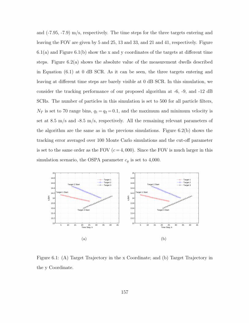
and (-7.95, -7.9) m/s, respectively. The time steps for the three targets entering and

leaving the FOV are given by 5 and 25, 13 and 33, and 21 and 41, respectively. Figure

6.1(a) and Figure 6.1(b) show the x and y coordinates of the targets at different time

steps. Figure 6.2(a) shows the absolute value of the measurement dwells described

in Equation (6.1) at 0 dB SCR. As it can be seen, the three targets entering and

leaving at different time steps are barely visible at 0 dB SCR. In this simulation, we

consider the tracking performance of our proposed algorithm at -6, -9, and -12 dB

SCRs. The number of particles in this simulation is set to 500 for all particle filters,

NT is set to 70 range bins, q1= q2=0.1, and the maximum and minimum velocity is

set at 8.5 m/s and -8.5 m/s, respectively. All the remaining relevant parameters of

the algorithm are the same as in the previous simulations. Figure 6.2(b) shows the

tracking error averaged over 100 Monte Carlo simulations and the cut-off parameter

is set to the same order as the FOV (c=4, 000). Since the FOV is much larger in this

simulation scenario, the OSPA parameter cg is set to 4,000.

5 10 15 20 25 30 35 40 4513

13.2

13.4

13.6

13.8

14

14.2

14.4

14.6

14.8

15

Time Step, k

x,km

Target 1 Start

Target 2 Start

Target 3 Start

Target 1Target 2Target 3

(a)

5 10 15 20 25 30 35 40 4513

13.2

13.4

13.6

13.8

14

14.2

14.4

14.6

14.8

15

Time Step, k

x,km

Target 1 Start

Target 2 Start

Target 3 Start

Target 1Target 2Target 3

(b)

Figure 6.1: (A) Target Trajectory in the x Coordinate; and (b) Target Trajectory in

the y Coordinate.

157

The tracking error is very small at -6 dB with slightly higher cardinality error

around the time when the targets are entering the FOV. The cardinality error is

higher at -9 dB, and the tracking error is very high at time steps 20–25 when all

the targets are present. This increased error is dominated mostly due to the delayed

detection of the third target, as the proximity of the first target is closer to the third

target’s initial position. Once a target is detected, the localization error is eventually

reduced as seen around the vicinity of time steps 6–10 and 25–30. The localization

error is generally low and the OSPA is limited by the range resolution. At -12 dB

SCR, the tracking performance of the algorithm degrades drastically and the joint

detection of all three targets becomes very difficult. Nevertheless, the algorithm is

able to detect at least one target, as evident by the relatively reduced tracking error

around time steps 8–12 and 33–40.

Dwell, k

Ran

ge, k

m

Target 1 Start

Target 2 Start

Target 3 Start

5 10 15 20 25 30 35 40 45

16

18

20

22

24

26

(a)

0 10 20 30 40 500

500

1000

1500

2000

2500

3000

3500

4000

Time, k

OS

PA

, m

scr=−6 dBscr=−9 dBscr=−12 dB

(b)

Figure 6.2: (A) Absolute Value of Measurement Dwells at 0 dB SCR. (b) Tracking

Error, OSPA(4000,2).

158

6.7.2 High Resolution Radar and Compound Gaussian Clutter

In this section, we discuss the simulation results for a simulated high resolu-

tion radar in compound Gaussian modeled clutter. The simulated radar parameters

are given in Table 6.3. Specifically, we compared the performance of our proposed

method with the two likelihood functions (LQ and CG-K) discussed in Section 6.4.

The speckle components were randomly generated from a complex Gaussian random

process whose correlation properties were estimated in [110] using real radar mea-

surements collected with the Osborne Head Gunnery Range (OHGR) IPIX radar

[161]. The texture was generated from a correlated gamma distributed random pro-

cess with scale bg and shape cg parameters [89]. We also used the texture correlation

estimated in [110]. The Doppler model parameters discussed in Section 6.3.3 are set to

µBragg =−15 Hz, σBragg =7.07 Hz, Aswell =50 Hz, Bswell =5.95 Hz. The standard devia-

tion σswell is randomly sampled from a Gaussian distribution with mean and standard

deviation equal to 60 Hz. The degree of spikiness of the texture component is con-

trolled by the shape parameter cg; decreasing cg results in more spiky clutter. The

averaged Doppler clutter spectrum for different values of cg is shown in Figure 6.3.

For higher cg values, the averaged Doppler spectrum is centered around the assumed

Bragg’s model parameters, whereas for lower values, the frequency centers around

the swell model parameters. Figure 6.4 shows the absolute value of the pulse Doppler

measurements for different values of cg. The targets are visible in Figure 6.4(a) for

cg = 10 at 3 dB SCR, however they are not clearly distinguishable as the cg value is

decreased. For cg = 0.2, a lot of target like clutter components can be observed. In

this case, for a given SCR over the entire FOV, the instantaneous SCR appears much

lower in some range bins for cg =0.2 when compared to cg =10. This phenomenon is

typical for high resolution radars because the reflected clutter power from a range bin

159

Table 6.3: Simulated High Resolution Radar System Parameters


Carrier frequency, fc 10 GHz

Baseband signal Linear FM pulse

Baseband bandwidth 25 MHz

Fast time sampling, fs 25 MHz

Pulse Width, Ns 10 samples

Pulse interval time, TPRI 500 µs

Validation range gate 15.25 km to 16.75 km

Number of valid range bins, Nr 249

Range resolution 6 m

Maximum radial velocity 30 m/s (108 km/hr)

DOA 45o

Beamwidth 0.703o

Cross-range resolution range 93.59 m

Beam scan rate 240 rotations per minute

Dwell interval 0.25 s

Number of pulses per dwell, Np 20

Motion model Constant velocity

is smaller than that of a low resolution radar because of fewer number of scatterers

in the physical area corresponding to a range bin.

We compared the performance of the algorithm for tracking three targets moving

at constant velocity. The targets are assumed to leave and enter the FOV at different

time instants (5 and 25 dwells, 13 and 33 dwells, 21 and 41 dwells for Targets 1, 2

160

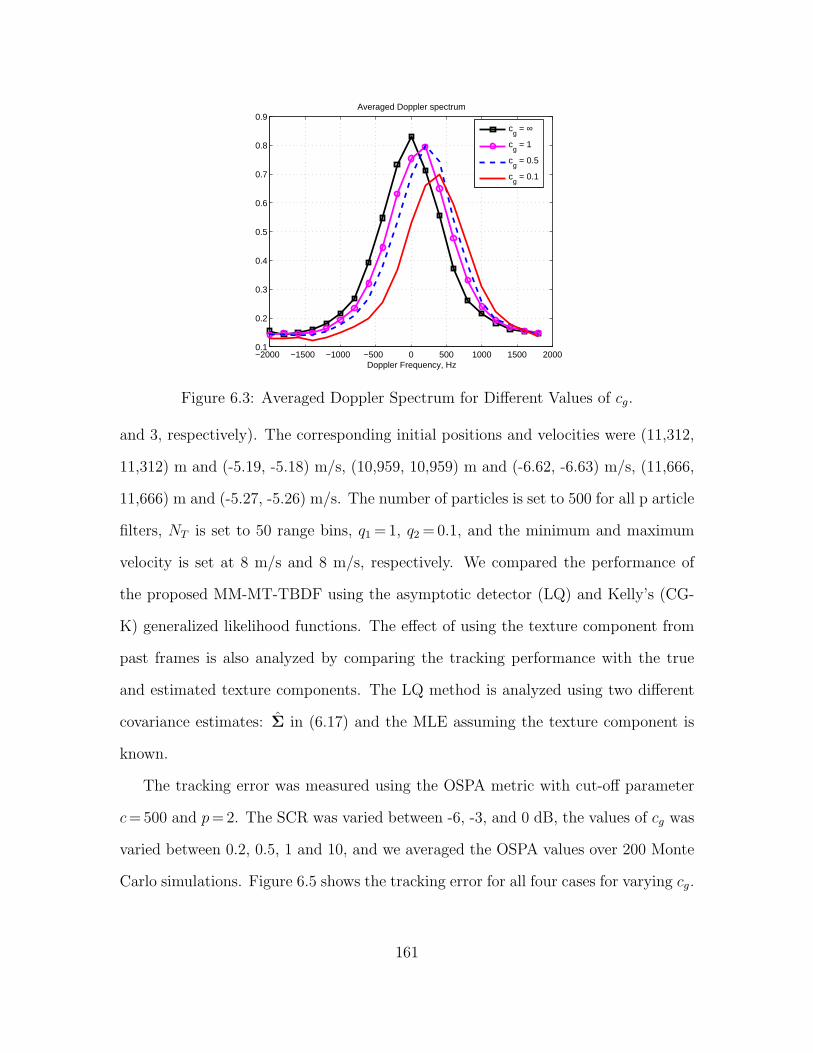
−2000 −1500 −1000 −500 0 500 1000 1500 20000.1

0.2

0.3

0.4

0.5

0.6

0.7

0.8

0.9

Doppler Frequency, Hz

Averaged Doppler spectrum

c

g = ∞

cg = 1

cg = 0.5

cg = 0.1

Figure 6.3: Averaged Doppler Spectrum for Different Values of cg.

and 3, respectively). The corresponding initial positions and velocities were (11,312,

11,312) m and (-5.19, -5.18) m/s, (10,959, 10,959) m and (-6.62, -6.63) m/s, (11,666,

11,666) m and (-5.27, -5.26) m/s. The number of particles is set to 500 for all p article

filters, NT is set to 50 range bins, q1=1, q2=0.1, and the minimum and maximum

velocity is set at 8 m/s and 8 m/s, respectively. We compared the performance of

the proposed MM-MT-TBDF using the asymptotic detector (LQ) and Kelly’s (CG-

K) generalized likelihood functions. The effect of using the texture component from

past frames is also analyzed by comparing the tracking performance with the true

and estimated texture components. The LQ method is analyzed using two different

covariance estimates: Σ in (6.17) and the MLE assuming the texture component is

known.

The tracking error was measured using the OSPA metric with cut-off parameter

c=500 and p=2. The SCR was varied between -6, -3, and 0 dB, the values of cg was

varied between 0.2, 0.5, 1 and 10, and we averaged the OSPA values over 200 Monte

Carlo simulations. Figure 6.5 shows the tracking error for all four cases for varying cg.

161

The CG-K performs the best for all values of cg. The CG-K has a similar performance

with the estimated and true texture for moderately spiky clutter, and the tracking

error averages around 30 m. The LQ performs poorly when the clutter is spiky for all

covariance matrix estimations. For cg =0.2, the CG-K tracking performance degraded

when using the past frame’s texture component, as compared to the true texture

component. However, the CG-K with estimated texture components still performed

better than LQ. Similarly, Figure 6.6 shows the tracking error for all four cases for

varying SCR. At -6 dB SCR, the LQ method performed better than the other two

methods but had more false alarms between dwells 41-46. The performance of the two

CG-K based methods was generally better than the two LQ methods at higher SCR.

The OSPA metric was higher during target mode transition periods (cardinality error)

that happened at dwells 5, 13, 20, 25, 33, and it indicated some delay in detecting a

target entering or leaving the FOV.

162

0

2

4

6

8

1015.4

15.615.8

1616.2

16.416.6

00.020.04

Range, km

Times, sec

RC

S

(a)

0

2

4

6

8

1015.4

15.615.8

1616.2

16.416.6

00.020.04

Range, km

Times, sec

RC

S

(b)

0

2

4

6

8

1015.4

15.615.8

1616.2

16.416.6

00.020.04

Range, km

Times, sec

RC

S

(c)

Figure 6.4: Fast Time Measurement, SCR=3 dB: (a) cg=10;(b) cg=0.5; (c) cg=0.2.

163

10 20 30 4010

1

102

Time, k

OS

PA

(2,5

00),

m

cg = 10

10 20 30 4010

1

102

Time, k

OS

PA

(2,5

00),

m

cg = 1

10 20 30 4010

1

102

Time, k

OS

PA

(2,5

00),

m

cg = 0.5

10 20 30 4010

1

102

Time, k

OS

PA

(2,5

00),

m

cg = 0.2

LQ(True τ)LQΣ

CG−KCG−K(True τ)

Figure 6.5: Tracking Error for Different Values of cg and SCR = 3 dB.

10 20 30 4010

1

102

Time, k

OS

PA

(2,5

00),

m

SCR = 3 dB

10 20 30 4010

1

102

Time, k

OS

PA

(2,5

00),

m

SCR = 0 dB

10 20 30 4010

1

102

Time, k

OS

PA

(2,5

00),

m

SCR = −3 dB

10 20 30 4010

1

102

Time, k

OS

PA

(2,5

00),

m

SCR = −6 dB

LQ(True τ)

LQΣ

CG−K

CG−K(True τ)

Figure 6.6: Tracking Error for Different Values of SCR and cg =0.5.

164

Chapter 7

ESTIMATION OF RAPIDLY-VARYING SEA CLUTTER USING NEAREST

KRONECKER PRODUCT APPROXIMATION

7.1 Rapidly-varying Sea Clutter Characterization

The detection and tracking of a target with low radar cross-section (RCS) in

maritime environments is an extremely challenging problem. The target’s kinematic

state estimation problem is complicated by reflections from fast moving sea waves,

causing target-like interference with substantial Doppler shifts. As a result, moving

target indicator methods, such as Doppler filtering [45], may not provide effective ways

to track a slow moving target in such environments. Various statistical modeling

based sea clutter characterization methods were used in combination with target

detection algorithms [126, 127, 162]. A principal component analysis based clutter

rejection technique was used in [109, 110] to improve target detection performance.

Experimental results indicated that sea clutter amplitude follows a long-tailed, non-

Gaussian distribution [100, 134, 135, 138]. The compound Gaussian (CG) distribution

is a well-established statistical model for characterizing the spiky nature of sea clutter

[89]. Using the CG model, the small scale structures on the sea surface are modeled as

speckle, following a complex Gaussian distribution with a short decorrelation time.

This speckle component is modulated by a slow varying texture component that

is associated with long sea waves and swell structures. Many adaptive detection

approaches applied the CG model with pulse integration, assuming knowledge of the

slow-time temporal covariance matrix of the range bin under testing [82, 85, 121,

123]. The sample covariance matrix estimate was derived by assuming statistical

165

independence between neighboring range bins [83, 84, 156]. However, using real data,

reflections from sea surface were found to be correlated over a distance of 100 m

[89]. Therefore, detection of targets using the space-time correlation properties of sea

clutter must be considered for optimal detection and tracking performance. Note that

space-time correlation properties include both temporal information (or measurement

from slow-time samples) as well as spatial information (or measurement from fast-

time samples) corresponding to the physical range location in the field-of-view (FOV)

of a radar from which the reflected signal has originated from.

A dynamic sea clutter model and a sea clutter space-time covariance matrix esti-

mation method were proposed in [163–165]. The dynamic state space model approach

to estimate sea clutter statistics is important in tracking the heterogeneity of the un-

derlying sea clutter. The validity of this state space model was also investigated

with real sea clutter. However, the practical feasibility of this algorithm in real-life

applications is not possible since it estimates all the elements of the covariance ma-

trix. The number of elements of the covariance matrix exponentially increases with

the number of range bins and the number of pulses used for coherent processing. In

addition to computational issues, the positive definiteness of the estimated matrix

cannot be ensured since the matrix elements are estimated by a set of independent

multiple particle filters. Moreover, the measurement model assumes the knowledge

of a noisy covariance matrix which was estimated by averaging a large number of

measurements.

In this chapter, we propose a modified clutter estimation algorithm to avoid the

aforementioned drawbacks by imposing a Kronecker product (KP) assumption on

the space-time covariance matrix [90, 91]. In the literature, many methods have

been proposed to estimate the covariance matrix when its structure is in the KP

form [166–168]. For example, the nearest KP approximation [169] was used in [170]

166

to approximate the space-time covariance matrix for wind speed data. In our pro-

posed method, we use the aforementioned sea clutter model and space-time covariance

matrix state model but we reformulate it such that the number of elements to be esti-

mated is drastically reduced due to KP assumption. A particle filter (PF) [17] based

implementation method is also proposed to estimate the matrix elements. In addi-

tion, our proposed model does not require a large number of measurements as the

likelihood function used to update the particle weights requires a significantly fewer

number of pulse Doppler measurements. Finally, the proposed method is guaranteed

to always provide a positive definite matrix solution. We provide an application of

our proposed method by extending the track-before-detect filter (TBDF) in [53] to

our measurement model by making use of the estimated space-time covariance ma-

trix and show improved tracking performance by comparing with the TBDF using

the compound Gaussian assumption.

7.2 Rapidly-varying Sea Clutter Model

7.2.1 Measurement Model

We consider the same pulse Doppler radar measurement model discussed in Sec-

tion 6.2. We assume that the same transmit signal is used within each dwell. At the

receiver, we assume that the region of measurement selection for track updates or

validation gate at the kth dwell consists of Nv = ζNv − ζ1 + 1 range bins. Assuming

no target is present, the noisy observation signal y(n/fs, p) from the pth pulse at the

kth dwell is sampled at fs Hz to obtain

yk[n, p] =n∑

m=n−Ns+1

ak[m, p]s[n−m] + wk[n, p] , (7.1)

where n= ζ1, . . . , ζNv + Ns − 1, p=0, . . . , Np − 1, wk[n, p] is assumed to be zero-

mean, white Gaussian observation noise at the kth dwell and pth pulse, the clutter

167

reflectivity ak[m, p] is defined as

ak[m, p] = ξk[m, p]ej2πνmpTPRI . (7.2)

where ξk[m, p] is the clutter reflectivity, and νm is the Doppler shift corresponding

to the clutter at the mth range bin. At the kth dwell, considering all Np pulses

and Nv + 2Ns − 1 range bins, the overall scatterer contribution is represented by

the ((Nv + 2Ns − 1) × Np) reflectivity matrix Ak defined in Equation (6.2) whose

(m, p)th element is ak[m, p]. In Section 6.2, a dwell measurement matrix consists of

an (Nv ×Np) matrix and this matrix correspond to reflectivity contribution from Nr

range bins, where Nr = Nv +Ns − 1. In this chapter, tracking is performed using the

measurement obtained by matched filtering the raw dwell measurement and therefore,

we require an (Nr ×Np) dwell measurement matrix that results from (Nv + 2Ns − 1)

range bins. Hence, we use more number of range bins in the reflectivity matrix Ak.

If a target is present, the signal in Equation (7.1) includes both the target and

clutter. If βk is the target reflectivity at range bin ζk, which is assumed unknown

[152], with Doppler shift νk, then the received measurement is

yk[n, p] = βk,ps[n− ζk] +n∑

m=n−Ns+1

ak[m, p]s[n−m] + wk[n, p].

where βk,p=βk exp(j2πνkpTPRI). Note that the range rk and range rate rk of the

target at the kth dwell are given by rk = ζkc/(2fs) and rk = νk c/(2fc), where c is

the velocity of propagation and fc Hz is the carrier frequency. In [163, 164], the

(N2rN

2p × N2

rN2p ) space-time clutter covariance matrix was obtained by estimating

the covariance matrix of the vectorized reflectivity matrix Ak. Note, however, that

estimating the covariance of the reflectivity matrix results in an increased number of

parameters to be estimated sinceNr range bins are needed to obtain the measurements

for Nv range bins. We reduced this complexity by directly estimating the covariance

168

of the matched filter output as this only requires Nv range bins. The output of the

matched filter is given by

zk[n, p] =n+Ns−1∑m=n

yk[m, p] s∗[m− n] (7.3)

for n= ζ1, . . . , ζNv , p=0, . . . , Np−1. Here, we use yk[n, p] as defined in Equation (7.1)

and assume that only clutter is present. The overall clutter measurements at the kth

dwell after matched filtering can be represented by the (Nv × Np) matrix Zk. The

matrix operation can be written in matrix form as

Zk = MYk (7.4)

where the (Nv ×Nr) matrix M is given by

M =

s∗[0] s∗[1] . . . s∗[Ns − 1] 0 . . . 0 0

0 s∗[0] s∗[1] . . . s∗[Ns − 1] 0 . . . 0

......

......

......

......

0 0 . . . 0 s∗[0] s∗[1] . . . s∗[Ns − 1]

and the (Nr × Np) raw pulse Doppler measurement matrix Yk at the kth dwell is

given by

Yk =

yk[ζ1, 0] yk[ζ1, 1] . . . yk[ζ1, Np − 1]

yk[ζ2, 0] yk[ζ2, 1] . . . yk[ζ2, Np − 1]

......

......

yk[ζNr , 0] yk[ζNr , 1] . . . yk[ζNr , Np − 1]

. (7.5)

7.2.2 Measurement State Space Model

As sea clutter is dynamically varying, its state transitions between adjacent range

bins depending on the relative velocity of sea waves with respect to the radar. A

169

dynamic model was proposed in [164] in which the spectral component of the received

signal is allowed to transition from one range bin to its adjacent bins depending on

the Doppler shift. Based on this model, the scattering matrix corresponding to the

(Nv ×Np) measured signal Zk in Equation (7.4) is obtained as

Bk = ZkD (7.6)

where D is an (Np × Np) discrete Fourier transform matrix. The elements of D are

such that the first (Np−1)/2 columns list the negative Doppler shifts, the middle

column is the zero Doppler shift, and the remaining columns list the positive Doppler

shifts. In this model, most of the sea clutter components can be shown to concentrate

around the middle column under calm sea state conditions but move away from the

middle column under turbulent conditions.

We represent the clutter state transition in vector form by stacking the columns

of Bk from left to right to form the (Nv Np × 1) vector, bk =vec(Bk). The operator

vec(·), vectorizes a matrix by stacking all the columns of the matrix. For exam-

ple, if Bk = [b1 b2 . . . bNp ], where bi is the ith (Nv × 1) column of matrix Bk, then

vec(Bk)= [bT1 bT

2 . . . bTNp]T. We similarly represent the matched filter output at the

kth dwell as the (NvNp × 1) vector zk =vec(Zk). Using the KP property A.2 in Ap-

pendix A [171], and Equation (7.6), the relation between the two vectors bk and zk

can be written as

bk = (DH ⊗ INv) zk

where H denotes Hermitian transpose and INv is the (Nv ×Nv) identity matrix. The

KP operator ⊗ computes the KP on the (Np × Np) matrix DH and the (Nv × Nv)

matrix INv to form an (Nv Np × Nv Np) block matrix. The measurement vector can

be obtained from the spectral vector as

zk = (D−H ⊗ INv)bk. (7.7)

170

The clutter state transition is modeled using the state equation as

bk+1 = Fbk + vk+1 (7.8)

where vk+1 is the modeling random error process assumed to be a zero-mean complex

Gaussian process with covariance Vk+1. The (Nv Np×Nv Np) state transition matrix

F (defined in Equation (9) in [164]) represents the scattering movement between

dwells and populates the range-Doppler bins moving into the validation gate. It

represents the transition of a fast moving clutter between range bins n and n + l if

the reflector is moving away from the radar and between range bins n and n − l if

the reflector is moving towards the radar; the value of l is determined by the Doppler

shift. Specifically, the state transition matrix F is an (Nv Np ×Nv Np) block diagonal

matrix constructed from (Nv × Nv) submatrices Fq. For negative Doppler shifts,

q=−(Np − 1)/2, . . . ,−1, [163–165]

Fq =

2|q|−1e−|q|γ 2|q|−1e−(|q|+1)γ . . . (2|q|−1 − 1)e−(Nv+1)γ . . . (2|q|−1 − |q|+ 1)e−(Nv+|q|−1)γ

......

......

......

2e−2γ 2e−3γ . . . . . . . . . e−(Nv+1)γ

e−γ e−2γ . . . . . . . . . e−Nvγ

1 0 . . . . . . . . . 0

......

......

......

0 . . . . . . 1 . . . 0

171

and for positive Doppler shifts, q=1, . . . , (Np − 1)/2

Fq =

0 . . . . . . 1 . . . 0

......

......

......

0 0 . . . . . . 1 0

0 0 . . . . . . 0 1

e−Nvγ . . . . . . . . . . . . e−γ

e−(Nv+1)γ . . . . . . . . . 2e−3γ 2e−2γ

......

...

(2|q|−1 − |q|+ 1)e−(Nv+|q|−1)γ . . . (2|q|−1 − 1)e−(Nv+1)γ . . . 2|q|−1e−(|q|+1)γ 2|q|−1e−|q|γ

.

For q=0, F0 is the (Nv × Nv) identity matrix since the clutter with zero Doppler

shifts does not transfer to adjacent range bins from dwell to dwell. The exponential

averaging parameter γ controls the contribution from neighboring range bins. Figure

7.1 shows the structure of the spectral matrix and indicates the transition of clutter

reflectivity between dwells. This state transition model was validated with real sea

clutter in [165].

7.2.3 Clutter Covariance Matrix State Space Model

In order to estimate the clutter measurement covariance matrix Σzk , we use the

relation between zk and bk to relate their corresponding covariance matrices Σzk and

Σbk. From Equation (7.8), the covariance matrix of bk+1 can be written as

Σbk+1= FHΣbk

F+Gk+1 (7.9)

172

1

2,

1

2,

1

2,

1

2,

Moving towards,

Positive Doppler shift

Moving

away,

Negative

Doppler

shift

Exponentially

weighted

contribution

from other

range bins

Doppler

Figure 7.1: Sea Clutter Covariance Transition Model for the Matrix in Equation (7.6).

where Gk+1 is assumed Wishart distributed with parameters Vk+1 and Nv Np degrees

of freedom, and

Σbk= (DH ⊗ INv)Σzk(D⊗ INv). (7.10)

Replacing Equation (7.10) in Equation (7.9), we obtain

Σbk+1= FH (DH ⊗ INv)Σzk(D⊗ INv)F+Gk+1. (7.11)

The covariance matrix Σzk+1 is obtained by using the relation in Equation (7.7),

Σzk+1 = (D−H ⊗ INv)Σbk+1(D−1 ⊗ INv). (7.12)

This covariance state space model is similar to the one in [164]. Thus, as the size

of the covariance matrix grows exponentially with Np and Nv, the estimation of the

covariance in Equation (7.11) becomes very computationally intensive.

7.2.4 Covariance Nearest Kronecker Product Approximation

In the measurement model described in Section 7.2.1, the rows and columns of the

raw fast time measurement can be modeled as a function of two random processes.

173

The rows of the measurement matrix can be treated as an (Np × 1) random vector,

qk, representing a temporal random process and the columns can be treated as an

((Nv + Ns − 1) × 1) random vector, ck, representing the spatial random process. In

particular, assuming that the temporal and spatial vectors have the same distribution

for all range bins and pulses, respectively, then we can model the measurement matrix

Yk in Equation (7.5) as the KP on the two random vectors using

Yk = qHk ⊗ ck . (7.13)

The above measurement matrix can be written in vector form yk = vec(Yk) as

yk = qk ⊗ ck.

Using the KP property A.1 in Appendix A [171], the covariance of yk can be written

as

Σyk= E[(qk ⊗ ck)(qk ⊗ ck)

H] = E[qkqHk ⊗ ckc

Hk]

= Σqk⊗Σck ,

where E[.] is the expectation operator. Therefore, if we assume that the underlying

physical process follows the KP form, then the covariance of the measurement is also

in the KP form. Thus, even though the underlying random process from which the

pulse Doppler measurement is obtained follows the KP form, we still need to ensure

that the KP form is preserved after matched filtering. The matched filter output

vector is shown to be related to the pulse Doppler measurement using Equation (7.4)

as

zk = (INp ⊗MNv×(Nv+Ns))yk

= (INp ⊗MNv×(Nv+Ns))(qk ⊗ ck)

=(qk ⊗Mck).

174

The covariance of zk can be simplified as

Σzk = E[(qk ⊗Mck)(qk ⊗Mck)H]

= E[qkqHk ⊗Mckc

HkM

H]

= Σqk⊗MΣckM

H

= Σqk⊗Σrk

(7.14)

where Σrk =MΣckMH. Thus, the matched filtered measurement also follows the KP

form when the raw pulse Doppler measurement is in KP form. The covariance matrix

of bk in Equation (7.10) can then be written in KP form as

Σbk= (DH ⊗ INv)(Σqk

⊗Σrk)(D⊗ INv) = Σtk ⊗Σrk

where Σtk =DHΣqkD. Substituting the above equation in Equation (7.9), the state

space model can be simplified as

Σbk+1= FH (Σtk ⊗Σrk)F+Gk+1 . (7.15)

In the above KP model, even if the covariance matrix Σbkat dwell k is in KP form,

the covariance matrix at dwell k + 1 does not have to be in KP form due to the

structure of the state transition matrix F. Using Equation (7.12), the covariance of

the matched filter output is given by

Σzk+1 = (D−H ⊗ INv)FH (Σtk ⊗Σrk)F(D−1 ⊗ INv) +

(D−H ⊗ INv)Gk+1(D−1 ⊗ INv).

(7.16)

In order to maintain the KP form for the covariance matrix of the measurement at the

(k+1)th dwell transition, we impose the following covariance constraint on Equation

(7.18),

Σzk+1= Σqk+1

⊗Σrk+1= arg min

Σqk+1,Σrk+1

∥ Σzk+1−Σqk+1

⊗Σrk+1∥F (7.17)

175

where ∥ · ∥F is the Frobenius matrix norm [172]. The minimization problem in

Equation (7.17) corresponds to a nearest KP approximation (NKPA) problem [169];

the solution is the cross product of the singular vector corresponding to the maximum

singular value of the permuted version of Σzk+1. Specifically, the covariance matrix

Σzk+1can be written as a block matrix using a set of (Nv × Nv) sized sub-matrices

Σ(i,j)

zk+1, representing the covariance matrix between the ith and jth columns of the

measurement matrix Zk+1. Specifically, the covariance matrix can be written as

Σzk+1=

Σ(1,1)

zk+1Σ

(1,2)

zk+1. . . Σ

(1,Np)

zk+1

...... . . .

...

Σ(Np,1)

zk+1Σ

(Np,2)

zk+1. . . Σ

(Np,Np)

zk+1

.

The (N2p ×N2

p ) permuted version of the block matrix is written as

Σ(p)

zk+1=

vec(Σ(1,1)

zk+1)H

...

vec(Σ(Np,1)

zk+1)H

vec(Σ(1,2)

zk+1)H

...

vec(Σ(Np,2)

zk+1)H

...

vec(Σ(Np,Np)

zk+1)H

.

According to the NKPA method, the original minimization problem in Equation

(7.17) is recasted into a modified minimization problem using the permuted matrix

176

as

Σzk+1= Σqk+1

⊗Σrk+1= arg min

Σqk+1,Σrk+1

∥ Σ(p)

zk+1− vec(Σqk+1

)vec(Σrk+1)H ∥F .

The solution to the above minimization problem is a singular value decomposition

problem in which the permuted matrix is approximated by a rank one matrix obtained

by the cross product between the left and right singular vectors corresponding to the

maximum singular value [172].

Thus, solving the minimization problem in Equation (7.17) using the NKPA re-

sults in a drastically reduced computational complexity in estimating the measure-

ment covariance matrix. Specifically, the NKPA reduces the number of matrix ele-

ments to be estimated from (NpNv(NpNv+1)/2) to [Np(Np+1)+Nv(Nv+1)]/2. For

example, if Np=10 pulses and Nv =10 range bins, the element estimation reduction

is from 5,050 to 110 elements.

7.3 Validation of KP Approximation Using Real Sea Clutter Measurement

We validated the KP form of the sea clutter covariance matrix using real clutter

data from the DSTO INGARA radar sea clutter database [138]. The clutter data was

obtained using the following radar parameter: 96 MHz signal bandwidth, 8 µs pulse

width, 9.375 GHz carrier frequency, 500 Hz pulse repetition frequency, 1.5 m range

resolution, and vertical-transmit, vertical-receive polarization. The wind speed was

at 10-12 knots, resulting in a 2-3 sea state [138]. As the true covariance matrix was

not available, the NKPA was validated using the sample covariance matrix, obtained

by averaging across multiple dwells and calculated by constructing a measurement

dwell with Np=10 pulses and Nv =10 range bins. Figure 7.2(a) shows the singular

values of the permuted sample covariance matrix computed by averaging over 4,000

dwells from 3 different data sets. The first singular value was the most dominant one

177

1 2 3 4 5 6 7 8 9 100

50

100

150

200

250

300

350

400

singular value index

singula

r va

lues

Data set #1Data set #2Data set #3

(a)

0 500 1000 1500 2000 2500 3000 3500 4000 45000.1

0.2

0.3

0.4

0.5

0.6

0.7

0.8

Number of dwells

NK

PA

Fro

be

niu

s e

rro

r

Data set #1Data set #2Data set #3Data set #4Data set #5

(b)

Figure 7.2: (a) Singular Value of the Permuted Covariance Matrix. (b) NKPA Error

for Different Number of Dwells for Estimating the Sample Covariance Matrix.

for all 3 sets, thus most of the energy could be compacted by a single NKPA. The

KP approximation quality is evaluated by calculating the normalized Frobenius error

[172] as

eF(Σzk ,Σzk) =∥ Σzk −Σzk ∥F

∥ Σzk ∥F.

Figure 7.2(b) shows the normalized Frobenius norm error between the sample co-

variance and the NKPA as a function of sample size. As it can be seen, the error

decreases as the number of samples increases implying that, as the sample covariance

matrix asymptotically approaches the true covariance matrix, the approximation er-

ror is reduced. The approximation error is less than 0.2 for all data sets, indicating

that the NKPA is a reasonable approximation to use.

178

7.4 Covariance Matrix Estimation Using Sequential Monte Carlo Technique

7.4.1 Estimation Approach

As the state model in Equation (7.15) is not linear, we use PF to estimate the co-

variance matrix elements [16]. The PF represents the spatial (Σrk) and the temporal

(Σqk) covariance matrices by a set of particles Σ(n)

rkand Σ(n)

qk, respectively, and corre-

sponding weights w(n), n = 1, . . . , N . Given the initial particle states, the predicted

matrices at dwell k + 1 are obtained using the state model in Equation (7.18). The

predicted particles are updated using the clutter measurement likelihood function.

Assuming that the clutter measurement vector in a dwell follows a circularly sym-

metric complex Gaussian distribution, and assuming that we have NT independent

and identically distributed dwells, the joint PDF of the measurement vector is given

by

p(zk, zk−1 . . . zk−NT|Σzk) =

1

πNpNvNT |Σzk |NTexp

[ k−1∑i=k−NT

−tr(Σ−1

zkziz

Hi

) ]where tr(·) is the trace of a matrix. Here, we assume that the clutter statistics do

not drastically change while the (NT + 1) measurements corresponding to past and

current dwells are acquired. Since we assumed that the covariance matrix of the

measurement is in KP form, i.e., Σzk = Σqk⊗Σrk , we obtain

p(zk, zk−1 . . . zk−NT|Σzk) =

|Σqk⊗Σrk |−NT

πNpNvNTexp

[ k∑i=k−NT

−tr((Σqk

⊗Σrk)−1ziz

Hi

) ]

=|Σqk

|−NTNv |Σrk |−NTNp

πNpNvNTexp

[−NT tr

((Σ−1

qk⊗Σ−1

rk)Σzk

)]where we used the KP properties A.4 and A.5 in Appendix A on any two square and

invertible matrices. The sample covariance matrix in KP form is obtained from the

179

measurement using the NKPA as

Σzk = arg minΣqk

,Σrk

∥ 1

NT

k−1∑i=k−NT

zizHi − Σqk

⊗ Σrk ∥F

Since the clutter can be fast varying, the number of samples used for the sample

covariance estimate is usually much smaller than the vector dimension, i.e., NT ≪

Np Nv. If we do not use the NKPA on the covariance matrix, the maximum likelihood

estimate (MLE) is the sample covariance matrix, which is positive definite only if

NT ≥ Np Nv. However, by assuming the NKPA, the MLE in KP form is positive

definite as long as NT ≥ max

Nv

Np, Np

Nv

+ 1 [173, 174].

Given the measurement vector, the particle weights are set proportional to the

likelihood function

w(n) ∝ l(zk| Σ(n)

qk,Σ(n)

rk

).

The likelihood function given the measurement vector can now be derived as

l(zk| Σ(n)

qk,Σ(n)

rk

)=

|Σqk|−Nv |Σrk |−Np

πNpNvexp

[− tr

((Σ(n)

qk)−1Σqk

⊗ (Σ(n)rk

)−1Σrk

)]

=|Σqk

|−Nv |Σrk |−Np

πNpNvexp

[− tr

((Σ(n)

qk)−1Σqk

)tr((Σ(n)

rk)−1Σrk

)]where we have used the KP property A.3 in Appendix A. Here, the likelihood func-

tion computation is simplified since we compute the inverse and determinant of two

matrices of low dimension instead of one matrix of higher dimension.

We demonstrate next that the positive definiteness of the covariance matrix esti-

mate is preserved. Assuming that the initial covariance matrices Σqk, Σrk and the

modeling error matrix Gk+1 are positive definite, then Σbk+1in Equation (7.15) is

also positive definite. Using Equation (7.10), Σzk+1in Equation (7.17) is also positive

definite since, for a symmetric positive definite matrix, the solution to the NKPA also

results in symmetric positive definite matrices [169]. Therefore, Σqk+1and Σck+1

in

180

Equation (7.17) are positive definite. Since all the particles correspond to positive

definite matrices, the updated particles also correspond to positive definite matrices.

This ensures that the proposed covariance matrix estimate is always positive definite.

7.4.2 Simulations

We demonstrated the PF implementation of the covariance estimation using an

linear frequency modulated (LFM) signal with bandwidth fs=15 MHz, fc=9.375

GHz carrier frequency, TPRI =2 ms, Np=11 pulses per dwell, Ns=6 samples, [8,000

8,300] m validation gate range, 10 m range resolution, 30 range bins and 60 rpm beam

scan rate. The initial covariance matrixΣz0 was obtain assuming compound Gaussian

distributed clutter whose speckle and texture correlation was based on real clutter

from the Osborne Head Gunnery Range (OHGR) IPIX radar [110, 161]. The speckle

samples were drawn from a circularly symmetric complex Gaussian distribution, and

the texture components were distributed based on a gamma distribution. The sample

covariance matrix was calculated from 3,300 independent dwell measurements. The

fast time clutter measurement was obtained by drawing samples from a complex

Gaussian distribution with the covariance matrix derived at each dwell using Equation

(7.17). Figure 7.3 shows the transitioned covariance matrices at dwells 5 and 40. As

can be seen from the figure, the covariance matrix structure at dwell 40 evolved

differently from dwell 5 in accordance with the selected state transition matrix F in

Equation (7.8).

We compared the mean-squared error (MSE) between the true and estimated

temporal and spatial covariance matrices using a varying number of (50, 100, 250,

and 500) particles in Figure 7.4, averaged over 25 Monte Carlo simulations. Also

shown is the tracking MSE for the sample covariance matrix and its corresponding

NKPA. The sample covariance matrix is obtained by averaging the measurement from

181

50 100 150 200 250 300

50

100

150

200

250

300

(a)

50 100 150 200 250 300

50

100

150

200

250

300

(b)

Figure 7.3: Sea Clutter Covariance Matrix: (a) Dwell 5; and (b) Dwell 40.

five dwells. The tracking MSE for the sample covariance matrix is much higher; the

MSE is somewhat reduced when the NKPA of the sample covariance matrix is used.

The tracking MSE of our proposed estimation approach outperformed the other two

methods. The improved performance of the covariance matrix estimation is due to

exploiting the underlying physical model of the sea structure using the transition

matrix F in Equation (7.8). Note that the tracking MSE can also be reduced by

increasing the number of particles.

7.5 Track-before-detect Filtering in Sea Clutter

7.5.1 Track-before-detect Filtering Formulation with Clutter

In this section, we use the proposed NKPA-based covariance matrix estimation

to track a low observable target in the presence of sea clutter. We consider a target

moving in a two-dimensional (2-D) plane with state vector xk = [xk xk yk yk]T, where

(xk, yk) and (xk, yk) are the 2-D Cartesian coordinates of the target position and

182

0 5 10 15 20 25 30 35 4010

−2

10−1

100

101

Dwell number

Est

ima

tion

Err

or

(Fro

be

niu

s)

Sample covariance error

Nearest KP error

Tracking error( 50 particle)




Figure 7.4: Covariance Matrix Estimation (Frobenius) Error

velocity, respectively, at the kth dwell. The target state is modeled as xk =Fxk−1 +

wk, where F is a state transition matrix for a constant velocity model described in

Equation (2.6) and wk is the modeling error.

The single target efficient PF based TBDF algorithm [53] described in Section

3.3 is modified for use with the measurement model. Using this algorithm, a target

leaving the FOV and a target already in the FOV are represented by two sets of

particles. The posterior probability density of the target is obtained as a weighted

combination of the particles from both sets. The measurement component associated

with the target is also present in the neighborhood of the range bin under testing (in

which the target is present). This component is governed by the correlation properties

of the transmitted signal [45]. Thus, detection and tracking must be performed using

all the neighborhood range bins, including the range bin under testing. Specifically,

183

for a target present at range bin ζk, the measurement data is extracted from the

measurement matrix Zk (that contains both the target and clutter) as

zk,ζk = vec

Zk[ζk −Nh, 0] Zk[ζk −Nh, 1] . . . Zk[ζk −Nh, Np − 1]

......

......

Zk[ζk, 0] Zk[ζk, 1] . . . Zk[ζk, Np − 1]

......

......

Zk[ζk +Nh, 0] Zk[ζk +Nh, 1] . . . Zk[ζk +Nh, Np − 1]

where Nh is the number of neighborhood bins. The covariance matrix Σzk,ζk

that

corresponds to this vector is a principal sub-matrix of the full covariance matrix

estimated in Section 7.2.4. This sub-matrix is also positive definite since any prin-

cipal sub-matrix of a positive definite matrix is also positive definite [172]. Figure

7.5 illustrates the extraction of a submatrix from a complete covariance matrix for

Nv =5, Nh=1 and ζk =3.

In an actual tracking application, estimating the clutter covariance matrix is a

challenging problem as the measurements include the target component. In practice,

the clutter is assumed homogeneous so that the clutter covariance can be estimated

using range bins in the neighborhood of the range bin under testing. If the clutter is

heterogeneous, then this assumption can lead to poor detection performance. Here,

we exploit the state space clutter model to predict the clutter covariance matrix

Σzk,ζkfrom the previous clutter covariance matrix estimate Σzk−k0,ζk

. Specifically,

we assume that the probability that the target is still present in range bin ζk at the

(k − k0)th dwell is very low. Thus, the sub-matrix Σzk,ζkcan be extracted from the

184

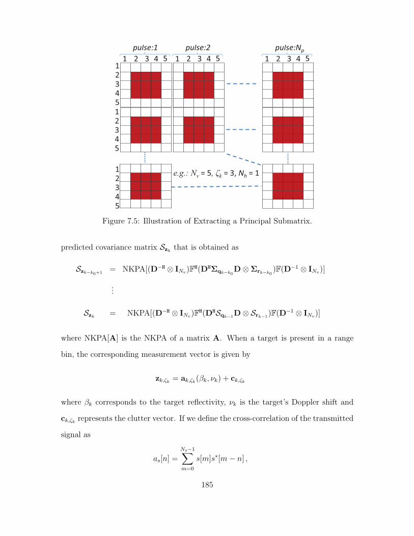
e.g.: Nv = 5, k = 3, Nh = 1

1

pulse:Np

2 3 4 5 1

pulse:2

2 3 4 5 1

pulse:1

2 3 4 5 1

2

3

4

5

1

2

3

4

5

1

2

3

4

5

Figure 7.5: Illustration of Extracting a Principal Submatrix.

predicted covariance matrix Szk that is obtained as

Szk−k0+1= NKPA[(D−H ⊗ INv)FH(DHΣqk−k0

D⊗Σrk−k0)F(D−1 ⊗ INv)]

...

Szk = NKPA[(D−H ⊗ INv)FH(DHSqk−1D⊗ Srk−1

)F(D−1 ⊗ INv)]

where NKPA[A] is the NKPA of a matrix A. When a target is present in a range

bin, the corresponding measurement vector is given by

zk,ζk = ak,ζk(βk, νk) + ck,ζk

where βk corresponds to the target reflectivity, νk is the target’s Doppler shift and

ck,ζk represents the clutter vector. If we define the cross-correlation of the transmitted

signal as

as[n] =Ns−1∑m=0

s[m]s∗[m− n] ,

185

then the signal vector ak,ζk is obtained by vectorizing the matrix formed by stacking

the vectors [as[m] as[m]ej2πνkTPRI . . . as[m]ej2πνk(Np−1)TPRI ]T, m=−Nh, . . . , Nh as

ak,ζk(βk, νk) = vec

βk

as[−Nh] as[−Nh]ej2πνkTPRI . . . as[−Nh]e

j2πνk(Np−1)TPRI

......

......

as[0] as[0]ej2πνkTPRI . . . as[0]e

j2πνk(Np−1)TPRI

......

......

as[Nh] as[Nh]ej2πνkTPRI . . . as[Nh]e

j2πνk(Np−1)TPRI

.

The detection and tracking is performed using the entirety of the selected vector

zk,ζk . Assuming that the clutter follows the circularly-symmetrix complex Gaussian

distribution, the likelihood ratio given a target state vector is given by

l(zk|xk) = exp−zHkS−1

zk,ζkzk + (zk − βkak)

HS−1zk,ζk

(zk − βkak)

= exp−|βk|2aHkS−1

zk,ζkak + 2ℜ

(β∗ka

HkS−1

zk,ζkzk)

where ℜ(.) denotes the real part of a complex number and for notational clarity, we

dropped the suffix ζk in zk,ζk and ak,ζk . The above likelihood ratio is a function of the

target reflectivity also. The argument inside the exponential function in the likelihood

ratio can be expanded as

−|βk|2aHkS−1k,ζk

ak + 2ℜ(β∗ka

HkS−1

k,ζkzk)

= −aHkS−1k,ζk

ak

∣∣∣∣βk −aHkS

−1k,ζk

zk

aHkS−1k,ζk

ak

∣∣∣∣2 + |aHkS−1k,ζk

zk|2

aHkS−1k,ζk

ak.

Since S−1k,ζk

is a positive definite matrix, aHkS−1k,ζk

ak > 0, and the exponential argument

is maximized only when

βk =aHkS−1

k,ζkzk

aHkS−1k,ζk

ak

.

186

The generalized likelihood function is derived by substituting this value of βk in the

likelihood function,

l(zk|xk) = exp

|aHkS

−1k,ζk

zk|2

aHkS−1k,ζk

ak

.

For real βk, the likelihood ratio is maximized when,

βk =ℜ(aHkS−1

k,ζkzk)

aHkS−1k,ζk

ak

and the corresponding generalized likelihood ratio is written as

l(zk|xk) = exp

[ℜ(aHkS

−1k,ζk

zk)]2

aHkS−1k,ζk

ak

.

The above derived likelihood ratio is used in the particle update stage of the efficient

PF based TBDF algorithm in Section 3.3.

7.5.2 Simulations

We applied the clutter estimation approach to a target tracking problem with

similar parameters as in the previous simulation. We compared the performance of

the algorithm to track a low observable target moving at constant velocity under

varying SCR values. The target is assumed to leave and enter the FOV at dwells

5 and 30, respectively. The initial position and velocity for the target were set to

(5,825.7, 5,825.7) m and (-5.4, -5.4) m/s, respectively. Figures 7.6(a), 7.6(b), and

7.6(c) show the measurement matrix for 9, 6, 3 dB SCRs, respectively. The target

is hardly visible at 6 dB and 3 dB SCR values and the clutter distribution is spiky

in nature with lots of target like components. Figure 7.7 shows the cross correlation

of the baseband signal for different time lags. The cross-correlation is dominated by

the correlation at zero time lag and it dominates even more when the bandwidth of

the baseband signal is increased. Since the main objective of the TBDF method is

187

0

5

10

15

20

25

30

35

88.05

8.18.15

8.28.25

0

0.1

0.2

Range, kmTimes, sec

RC

S

(a)

0

5

10

15

20

25

30

35

88.05

8.18.15

8.28.25

0

0.1

0.2

Range, kmTimes, sec

RC

S

(b)

0

5

10

15

20

25

30

35

88.05

8.18.15

8.28.25

0

0.1

0.2

Range, kmTimes, sec

RC

S

(c)

Figure 7.6: Pulse Doppler Radar Measurements: (a) SCR = 9dB; (b) SCR = 6 dB;

and (c) SCR = 3 dB.

to track a target under low SCR conditions, the low energy cross-correlation values

do not significantly contribute to the detection of a target in the presence of high

clutter, we thus set Nh = 3.

−5 0 5−1

0

1

2

3

4

5

6

Lag, samples

Cro

ss−c

orre

latio

n of

bas

eban

d si

gnal

realimaginary

Figure 7.7: Cross-Correlation of the Baseband Signal.

The PF used 500 particles when the target survived and 2,500 particles when the

target entered the FOV. The tracking error is quantified using the OSPA metric with

parameters c=100 and p=2 [105], averaged over 25 Monte Carlo simulations. The

188

tracking performance was analyzed under two conditions: (i) the measurement was

generated as in Equation (7.10) and the covariance was estimated using Equations

(7.15) and (7.17); (ii) both the measurement and the covariance followed the NKPA

in Equations (7.15) and (7.17). Figures 7.11(a) and 7.11(c) show the probability of

target existence and the tracking error for different SCRs. The latency in detecting

a target increased as the SCR decreased. Similarly, there was delay in detecting a

target leaving the FOV. The probability of detection was very low at 3 dB SCR and

the tracking error was high. As the probability of detection was in general low, the

probability of detecting a target leaving the FOV at 3 dB was also low, as evident

by lower OSPA values during dwells 30-35. At 6 dB SCR, the probability of detec-

tion increased when the true model did not follow the NKPA; however, this did not

result in improved tracking performance due to the higher OPSA values. In general,

the tracking performance improved when the true and assumed models followed the

NKPA. Nevertheless, the performance did not degrade significantly when the assumed

(but not the true) model followed the NKPA. This result is relevant to real target

tracking applications since, even if the actual covariance does not completely follow

the KP structure, we can apply the NKPA without significantly affecting the tracking

performance.

In the next simulation, we compare the tracking performance of the NKPA method

with a TBDF method discussed in the previous chapter. Specifically, we used the

asymptotic, linear quadratic (LQ) method discussed in Section 6.5.1 with the com-

pound Gaussian assumption (CG-LQ). The covariance matrix for the likelihood func-

tion in Equation (6.16) is estimated using the normalized sample covariance method

in Equation (6.19). The measurements are generated such that the KP property is

not maintained. Figure 7.9 compares the tracking performance at 12, 9, 6 and 3 dB

SCR conditions. The tracking performance of both the NKPA and CG-LQ methods

189

0 5 10 15 20 25 30 35 40 450

0.1

0.2

0.3

0.4

0.5

0.6

0.7

0.8

0.9

1

Dwell, k

Pro

ba

bili

ty o

f ta

rget

exi

ste

nce

scr=9 dBscr=6 dBscr=3 dB

(a)

0 5 10 15 20 25 30 35 400

10

20

30

40

50

60

70

80

90

100

Dwell, k

OS

PA

, m

scr=9 dBscr=6 dBscr=3 dB

(b)

Figure 7.8: (a) Probability of Target Existence; and (b) Tracking Error for Varying

SCR: True and Assumed KP Models (Solid), and Assumed KP Model Only (Dash).

0 5 10 15 20 25 30 35 40 450

0.2

0.4

0.6

0.8

1

1.2

Time, k

Pro

babili

ty o

f ta

rget exi

stence

scr=12 dB scr=9 dB scr=6 dB scr=3 dB

(a)

0 5 10 15 20 25 30 35 400

20

40

60

80

100

120

Time, k

OS

PA

, m

scr=12 dB scr=9 dB scr=6 dB scr=3 dB

(b)

Figure 7.9: (a) Probability of Target Existence; and (b) Tracking Error for Varying

SCR: KP (Solid) and CG-LQ (Dash).

are comparable at 12 dB SCR. At lower SCR conditions, the target existence proba-

bility shown in Figure 7.9(a) is very different between the two methods. Specifically,

190

the CG-LQ method with the independent range bin assumption results in very poor

detection performance when the range bins in the measurement are correlated. On

the other hand, the NKPA method processed with the space-time covariance matrix

produces a much improved detection performance. The tracking performance shown

in Figure 7.9(b) also follows a similar trend. Specifically, the tracking error using the

NKPA method becomes significantly higher at 3 dB SCR, whereas with the CG-LQ

method, the performance starts to deteriorate at 6 dB SCR. Therefore, by using the

estimated space-time covariance matrix, we can expect to get improved detection and

tracking performance.

0

1

2

3

4

58.22

8.238.24

8.258.26

0.20.40.60.8

Range, km

Times, sec

RC

S

(a)

5 10 15 20 25 30 35 400

0.2

0.4

0.6

0.8

1

1.2

Time, k

Pro

babili

ty o

f ta

rget exi

stence

12 dB 9 dB 6 dB

(b)

Figure 7.10: (a) Real Sea Clutter Embedded with Synthetic Target at 12 dB SCR; and

(b) Probability of Target Existence Probability Comparison with Real Sea Clutter:

KP (Solid) and CG-LQ (Dash).

In the next simulation, we used the real sea clutter measurement from the IPIX

radar described in Section 7.3 in which the pulse width of the radar is Ns = 800

samples. The measurement corresponding to the target is synthetically generated

using the same parameters used in the IPIX radar. The FOV is set at [8,220 8,268.5]

191

m resulting in 33 range bins at 1.5 m resolution and the number of pulses used for

coherent processing is set at Np = 11 and Nh=1. The (33×11) clutter measurements

are obtained using Equation (7.4) by matched filtering the raw measurements from

832 range bins that are extracted from the real recordings. The target associated

measurement dwells are synthesized from the reflectivity matrix that contains 1632

range bins. The initial states for the target is set at (5,839.8 5,839.8) m and (-5.4 -5.4)

m/s, and the target enters and leaves the FOV at time steps 5 and 30, respectively.

Figure 7.10(a) shows the real sea clutter mixed with the synthetic target associated

measurement at 12 dB SCR. The tracking performance of the NKPA and the CG-LQ

methods is compared at 12, 9 and 6 dB SCR conditions at the matched filter output.

The tracking performance was compared by setting the OSPA parameters to c=40

and p=2. Figure 7.10(b) shows the estimated target existence probability for both

methods. As the clutter level is increased, it takes more time to detect the target

with both methods. However, the detection rate of the CG-LQ method is significantly

worse at 9 and 6 dB SCR. Figure 7.11 shows the corresponding tracking performance

for both methods. When compared with the NKPA method, the CG-LQ method

takes more time to detect a target when the SCR is reduced. Moreover, at 6 dB SCR,

the localization error is also poor in addition to an increased cardinality error. Thus,

for real sea clutter measurements, the NKPA method provides promising results when

compared with the CG-LQ method in which the clutter statistics are computed from

the neighbourhood range bins that are not independent of each other.

192

0 5 10 15 20 25 30 35 400

5

10

15

20

25

30

35

40

Time, k

OS

PA

(40

,2)

NKPACG−LQ

(a)

0 5 10 15 20 25 30 35 400

5

10

15

20

25

30

35

40

Time, k

OS

PA

(40

,2)

NKPACG−LQ

(b)

0 5 10 15 20 25 30 35 400

5

10

15

20

25

30

35

40

Time, k

OS

PA

(40

,2)

NKPACG−LQ

(c)

Figure 7.11: Tracking Error Comparison with Real Sea Clutter: (a) SCR=12 dB; (b)

SCR = 9 dB; and (c) SCR = 6 dB.

193

Chapter 8

CONCLUSION AND FUTURE WORK

8.1 Conclusion

In this thesis, we derived a track-before-detect filter (TBDF) algorithm to track

a varying number of targets under low signal-to-noise ratio (SNR) and low signal-to-

clutter ratio (SCR) conditions that can be implemented using sequential Monte Carlo

(SMC) techniques. The multiple target TBDF estimates the target states under all

possible target existence combinations or modes using the derived multiple target joint

posterior probability density function. The resulting multiple mode multiple target

TBDF (MM-MT-TBDF) approach can keep track of targets entering or leaving a

scene, and only the maximum number of targets over the duration of a track needs to

be assumed known; the value of this number can be selected based on the application.

As we demonstrated, the proposed MM-MT-TBDF algorithm resulted in adequate

tracking performance, using the OSPA metric, when the SNR was as low as 0 dB.

The algorithm was also shown to successfully track a much larger number of targets

than other proposed methods in the literature. We also demonstrate that the MM-

MT-TBDF performed better when compared to the probability hypothesis density

TBDF for a simulation example using image measurements.

The MM-MT-TBDF is computationally expensive as most multiple target tracking

algorithms due to the large number of combinatorial choices that need to be com-

puted. In order to reduce the computational complexity without greatly affecting the

tracking accuracy under severe tracking conditions, we introduced various techniques

such as partition based proposal sampling. One of the inherent disadvantages with

194

the proposed algorithm is that the number of modes can grow exponentially as a

function of the maximum number of targets. We mitigated this problem by using a

decision-directed approach in which the estimated mode transition and target pres-

ence probabilities are used to control whether to run a particle filter that corresponds

to a particular mode transition. By using the decision-directed approach, the com-

putational load becomes a linear function of the maximum number of targets. This

problem can be further simplified by dynamically changing the maximum number of

targets. Specifically, the maximum number of targets can be increased or decreased

depending on the current estimate of the number of targets.

The computational load of the MM-MT-TBDF approach is also affected by the

significant number of new particles required to accurately detect when a new target

enters the field of view (FOV). This large number of particles is required as no a

priori information is assumed on the new target. Techniques such as constrained

particles filters [107] that assume that the kinematic state of a target that follows

a pre-determined pattern can be easily integrated into our method. The a priori

information used in knowledge aided radars [175] can also be exploited to reduce

the number of new particles. The algorithm architecture of the MM-MT-TBDF

also allows the implementation of the multiple particle filters (PFs) in a parallel

computing system [176]. Since the mode conditioned particle filters are independent

of each other, our proposed algorithm can run faster in a parallel computing system.

Moreover, the algorithm architecture also provides flexibility in assigning different

number of particles to approximate different mode-conditioned density functions.

In this thesis, we established a new paradigm for multiple target tracking based

on target existence modes that is not restricted to low SNR conditions as originally

designed for. Multiple target tracking with a dynamically varying number of targets

is a difficult problem both for low and high SNRs. The MM-MT-TBDF can also be

195

used under high SNR conditions, and we demonstrated that for a given number of

particles, the tracking error reduces, as the SNR increases. We can therefore deduce

that at higher SNR scenarios, we need a much smaller number of particles than when

for tracking low observable targets. Thus, under high SNR conditions, the algorithm’s

computational complexity can be further reduced by adjusting the number of particles

used in each PF.

When conventional detect before track methods are used to track targets in the

presence of clutter, they assume certain average number of clutters per measurement,

spatial distribution of clutter and probability of detection. Our proposed algorithm

does not require knowledge of these model parameters as we can integrate it with

methods to directly estimate clutter parameters from the measurements. We investi-

gate the performance of the algorithm in both low and high resolution radars, and in

particular, we concentrated on tracking scenes with high resolution radar in sea clutter

environment. We used the sea clutter compound Gaussian model at different levels of

sea spikes and clutter intensity levels. We also demonstrated the tracking capability

of our algorithm for slow moving target scenarios, where a simple Doppler domain

filtering cannot significantly improve tracking performance. The texture component

of the compound Gaussian model is assumed deterministic and a generalized likeli-

hood function is derived along with the maximum likelihood estimate of time varying

deterministic texture. The improved tracking performance of this generalized likeli-

hood function is then demonstrated by comparing with the tracking performance of

the conventional sub-optimal likelihood function that assumes random texture com-

ponent. One of the many challenges of target tracking in clutter is the estimation of

clutter statistics. As most clutter parameter estimation methods use neighbourhood

range and range rate bins, both target detector and tracker performance significantly

degrade if the clutter is non-homogeneous in nature. We provided a state space model

196

based approach to dynamically track the space-time covariance matrix of clutter and

used the Kronecker product (KP) assumption to reduce the computational complexity

of the covariance estimation algorithm.

8.2 Future Work

The KP approximation error for the space-time covariance matrix can be improved

further by decomposing the space-time covariance matrix into a sum of many KP

matrices [177]. Recent efforts in knowledge aided radars provide some promising

results in accurately estimating the clutter covariance matrix [178, 179]. We thus

plan to investigate some of these results in order to extend our KP approach to

non-homogeneous clutter in a knowledge aided radar framework [180]. Although the

compound Gaussian model has been proven to provide and adequate characterization

of the sea clutter, we need to investigate more dynamic models [165] to track the fast

varying nature of sea clutter. The proposed multiple target method can also be

extended to support agile radar processing similar to the method described for single

target TBDF in [104]. Finally, our proposed algorithm can be easily modified to

include some of the methods already developed to support realistic radar applications.

Specifically, the algorithm can be modified to support fluctuating target associated

signal intensity [55], Rayleigh measurement noise [53], complex measurements [56]

and dependent measurements [181].

197

REFERENCES

[1] R. E. Kalman, “A new approach to linear filtering and prediction problems,”Transactions of the ASME, Journal of Basic Engineering, vol. 1, pp. 35–45,March 1960.

[2] V. Chandrasekar and B. Zafar, “Precipitation type determination from space-borne radar observations,” IEEE Transactions on Geoscience and Remote Sens-ing, vol. 42, pp. 2248–2253, October 2004.

[3] L. Mu, T. Xiangqian, S. Ming, and Y. Jun, “Research on key technologiesfor collision avoidance automotive radar,” in IEEE Symposium on IntelligentVehicles, pp. 233–236, June 2009.

[4] D. E. Sturim, M. S. Brandstein, and H. F. Silverman, “Tracking multiple talk-ers using microphone-array measurements,” IEEE International Conference onAcoustics, Speech, and Signal Processing, vol. 1, pp. 371–374, April 1997.

[5] C. Wang and M. S. Brandstein, “Multi-source face tracking with audio andvisual data,” Third IEEE Workshop on Multimedia Signal Processing, pp. 169–174, 1999.

[6] H. G. Okuno, K. Nakadai, K. I. Hidai, H. Mizoguchi, and H. Kitano, “Human-robot interaction through real-time auditory and visual multiple-talker track-ing,” IEEE International Conference on Intelligent Robotics and Systems, vol. 3,pp. 1402–1409, 2001.

[7] S. Churchill, C. Randell, D. Power, and E. Gill, “Data fusion: Remote sensingfor target detection and tracking,” IEEE International Proceedings on Geo-science and Remote Sensing Symposium, vol. 1, pp. 609–612, September 2004.

[8] A. P. Goobic, M. E. Welser, S. T. Acton, and K. Ley, “Biomedical applicationof target tracking in clutter,” Thirty-Fifth Asilomar Conference on Signals,Systems and Computers, vol. 1, pp. 88–92, 2001.

[9] Y. Bar-Shalom, X.-R. Li, and T. Kirubarajan, Estimation with Applications toTracking and Navigation. Wiley-Interscience, 2001.

[10] H. W. Sorenson, Kalman Filtering: Theory and Application. IEEE Press, 1985.

[11] J. Sklansky, “Optimizing the dynamic parameter of a track-while-scan system,”RCA Review, vol. 18, pp. 163–185, July 1957.

[12] T. R. Benedict and G. W. Bordner, “Synthesis of an optimal set of radartrack-while-scan smoothing equations,” IRE Transaction on Automatic Con-trol, vol. AC-1, July 1962.

[13] P. R. Kalata, “α-β tracking systems: A survey,” American Control Conference,pp. 832–836, June 1992.

198

[14] M. Athans, R. Wishner, and A. Bertolini, “Suboptimal state estimation forcontinuous-time nonlinear systems from discrete noisy measurements,” IEEETransactions on Automatic Control, vol. 13, pp. 504–514, October 1968.

[15] S. Arulampalam, S. Maskell, N. Gordon, and T. Clapp, “A tutorial on particlefilters for on-line non-linear/non-Gaussian Bayesian tracking,” IEEE Transac-tions on Signal Processing, vol. 50, pp. 174–188, 2001.

[16] A. Doucet, N. de Fretias, and N. Gordon, Sequential Monte Carlo Methods InPractice. Springer-Verlag, NY, 2001.

[17] B. Ristic, S. Arulampalam, and N. Gordon, Beyond the Kalman Filter: ParticleFilters for Tracking Applications. Artech House Publishers, Boston, MA, 2004.

[18] S. Blackman and R. Popoli, Design and Analysis of Modern Tracking System.Artech House Publishers, New York, NY, 1999.

[19] Y. Bar-Shalom and X.-R. Li, Multisensor Tracking: Principles and Techniques.YBS Publishing, New York, NY, September 1995.

[20] Y. Bar-Shalom and T. E. Fortman, Tracking and Data Association. Orlando,FL: Academic, 1988.

[21] A. Farina and S. Pardini, “Track-while-scan algorithm in a clutter environ-ment,” IEEE Transactions on Aerospace and Electronic Systems, vol. AES-14,pp. 769–779, September 1978.

[22] P. Smith and G. Buechler, “A branching algorithm for discriminating andtracking multiple objects,” IEEE Transactions on Automatic Control, vol. 20,pp. 101–104, February 1975.

[23] Y. Bar-Shalom and E. Tse, “Tracking in cluttered environment with probabilis-tic data association,” Automatica, vol. 11, pp. 451–460, 1975.

[24] T. Kirubarajan and Y. Bar-Shalom, “Probabilistic data association techniquesfor target tracking in clutter,” Proceedings of IEEE, vol. 92, no. 3, pp. 536–557,March 2004.

[25] Y. Bar-Shalom, F. Daum, and J. Huang, “The probabilistic data associationfilter,” IEEE Controls System Magazine, pp. 82–100, December 2009.

[26] N. Gordon, “A hybrid bootstrap filter for target tracking in clutter,” IEEETransactions on Aerospace and Electronic Systems, vol. 33, pp. 353–358, 1997.

[27] G. W. Pulford, “Taxonomy of multiple target tracking methods,” IEE Pro-ceedings of Radar Sonar and Navigation, vol. 152, no. 5, pp. 291–304, October2005.

[28] D. Reid, “An algorithm for tracking multiple targets,” IEEE Transactions onAutomation and Control, vol. 24,6, pp. 84–90, 1979.

199

[29] S. S. Blackman, “Multiple hypothesis tracking for multiple target tracking,”IEEE Aerospace and Electronics Systems Magazine, vol. 19, no. 1, pp. 5–18,January 2004.

[30] T. E. Fortman, Y. Bar-Shalom, and M. Scheffe, “Sonar tracking of multipletargets using joint probabilistic data association,” IEEE Journal of OceanicEngineering, vol. 8, pp. 173–184, 1983.

[31] D. Sculz, W. Burgard, D. Fox, and A. B. Cremers, “Tracking multiple mov-ing targets with a mobile robot using particle filters and statistical data as-sociation,” Proceeding of the IEEE International Conference on Robotics andAutomation, vol. 2, pp. 1665–1670, 2001.

[32] D. Sculz, W. Burgard, and D. Fox, “People tracking with mobile robots usingsample-based joint probabilistic data association filters,” International Journalof Robotics Research 22, vol. 2, pp. 99–116, 2003.

[33] S. Godsill, J. Vermaak, and P. Perez, “Monte Carlo filtering for multi-targetand data association,” IEEE Transactions on Aerospace and Electronic Systems,vol. 41, no. 1, pp. 309–332, January 2005.

[34] W. Ng, J. Li, S. Godsill, and J. Vermaak, “A review of recent results in multipletarget tracking,” Proceedings of the 4th International Symposium on Image andSignal Processing and Analysis, pp. 40–45, September 2005.

[35] R. P. S. Mahler, “Random set theory for target tracking and identification,” inHandbook of multisensor data fusion (D. L. Hall and J. Llinas, eds.), pp. 1–33,Cambridge: CRC Press, 2001.

[36] R. P. S. Mahler, Statistical Multisource-Multitarget Information Fusion. Nor-wood, MA, USA: Artech House, Inc., 2007.

[37] B.-N. Vo, S. Singh, and A. Doucet, “Sequential Monte Carlo methods for mul-titarget filtering with random finite sets,” IEEE Transactions on Aerospace andElectronic Systems, vol. 41, no. 4, pp. 1224–1245, 2005.

[38] R. Mahler, “Objective functions for Bayesian control-theoretic sensor manage-ment, 1: multitarget first-moment approximation,” in Proceedings of the IEEEAerospace Conference, vol. 4, pp. 1905–1923, 2003.

[39] R. P. S. Mahler, “Multitarget Bayes filtering via first-order multitarget mo-ments,” IEEE Transactions on Aerospace and Electronic Systems, vol. 39, no. 2,pp. 1152–1178, 2003.

[40] B.-T. Vo, B.-N. Vo, and A. Cantoni, “The cardinality balanced multi-targetmulti-Bernoulli filter and its implementations,” IEEE Transactions on SignalProcessing,, vol. 57, pp. 409–423, February 2009.

[41] B.-N. Vo and W.-K. Ma, “The Gaussian mixture probability hypothesis densityfilter,” IEEE Transactions on Signal Processing, vol. 54, no. 11, pp. 4091–4104,2006.

200

[42] B.-N. Vo, A. Pasha, and H. D. Tuan, “A Gaussian mixture PHD filter fornonlinear jump Markov models,” in Forty-Fifth IEEE Conference on Decisionand Control, pp. 3162–3167, 2006.

[43] S. Julier and J. Uhlmann, “Unscented filtering and nonlinear estimation,” Pro-ceedings of IEEE, vol. 92, no. 3, pp. 401–422, 2004.

[44] H. Sidenbladh, “Multi-target particle filtering for the probability hypothesisdensity,” in Proceedings of the Sixth International Conference of InformationFusion, vol. 2, pp. 800–806, 2003.

[45] M. A. Richards, Fundamentals of Radar Signal Processing. New York: McGraw-Hill, 2005.

[46] S. M. Kay, Fundamentals of Statistical Signal Processing, Volume 2: DetectionTheory. New Jersey: Prentice-Hall Inc, 1993.

[47] M. Skolnik, Introduction to Radar Systems. New York: McGraw-Hill, 3rd ed.,2001.

[48] G. Richards, “Application of the Hough transform as a track-before-detectmethod,” in Target Tracking and Data Fusion (Digest No: 1996/253), IEEColloquium on, pp. 1–3, November 1996.

[49] W. Yi, L. Kong, J. Yang, and X. Deng, “A tracking approach based on dynamicprogramming track-before-detect,” in IEEE Radar Conference, pp. 1–4, May2009.

[50] S. M. Tonissen and Y. Bar-Shalom, “Maximum likelihood track-before-detectwith fluctuating target amplitude,” IEEE Transactions on Aerospace and Elec-tronic Systems, vol. 34, no. 3, pp. 796–809, July 1998.

[51] D. J. Salmond and H. Birch, “A particle filter for track-before-detect,” In Pro-ceedings of the American Control Conference, pp. 3755–3760, 2001.

[52] Y. Boers and H. Driessen, “Particle filter based detection for tracking,” InProceedings of the American Control Conference, pp. 4393–4397, Arlington,VA, USA, June 2001.

[53] M. G. Rutten, N. J. Gordon, and S. Maskell, “Efficient particle-based track-before-detect in Rayleigh noise,” International Conference on Information Fu-sion, pp. 693–700, June 2004.

[54] M. G. Rutten, B. Ristic, and N. J. Gordon, “Comparison of particle filters forrecursive track-before-detect,” International Conference on Information Fusion,pp. 169–175, 2005.

[55] M. G. Rutten, N. J. Gordon, and S. Maskell, “Recursive track-before-detectwith target amplitude fluctuations,” IEE Proceedings of Radar, Sonar and Nav-igation, vol. 52, no. 5, pp. 345–352, October 2005.

201

[56] S. J. Davey, B. Cheung, and M. G. Rutten, “Track-before-detect for sensorswith complex measurement,” Proceedings of the 12th International Conferenceon Information Fusion, pp. 619–625, Seattle, WA, July 2009.

[57] Y. Boers and H. Driessen, “Multitarget particle filter track before detect appli-cation,” IEE Proceedings of Radar, Sonar and Navigation, vol. 151, pp. 351–357,December 2004.

[58] M. Taj and A. Cavallaro, “Multi-camera track-before-detect,” IEEE Interna-tional Conference on Distributed Smart Cameras, pp. 1–6, September 2009.

[59] S. Buzzi, M. Lops, L. Venturino, and M. Ferri, “Track-before-detect proceduresin a multi-target environment,” IEEE Transactions on Aerospace and ElectronicSystems, vol. 44, no. 3, pp. 1135–1150, 2008.

[60] M. Fallon and S. Godsill, “Multi target acoustic source tracking using trackbefore detect,” in IEEE Workshop on Applications of Signal Processing to Audioand Acoustics, pp. 102–105, 2007.

[61] P. Pertila and M. S. Hamalainen, “A track before detect approach for sequentialBayesian tracking of multiple speech sources,” IEEE International Conferenceon Acoustics, Speech and Signal Processing, pp. 4974–4977, 2010.

[62] F. Lehmann, “Recursive Bayesian filtering for multitarget track-before-detectin passive radars,” IEEE Transactions on Aerospace and Electronic Systems,vol. 48, no. 3, pp. 2458–2480, 2012.

[63] F. Papi, B.-T. Vo, M. Bocquel, and B.-N. Vo, “Multi-target track-before-detectusing labeled random finite set,” in International Conference on Control, Au-tomation and Information Sciences,, pp. 116–121, November 2013.

[64] B. Ristic, D. Clark, and B.-N. Vo, “Improved SMC implementation of the PHDfilter,” in Thirteenth Conference on Information Fusion, pp. 1–8, 2010.

[65] K. Panta, B. Vo, and S. Singh, “Improved probability hypothesis density (PHD)filter for multitarget tracking,” in Third International Conference on IntelligentSensing and Information Processing (ICISIP), pp. 213–218, 2005.

[66] K. Punithakumar, T. Kirubarajan, and A. Sinha, “A sequential Monte Carloprobability hypothesis density algorithm for multitarget track-before-detect,”in Proceedings SPIE: Signal and Data Processing of Small Targets, vol. 5913,pp. 1–8, September 2005.

[67] R. Zhan and J. Zhang, “Improved multitarget track-before-detect for imagemeasurements,” in Eleventh IEEE International Conference on Signal Process-ing, vol. 3, pp. 2183–2187, 2012.

[68] B. K. Habtemariam, R. Tharmarasa, and T. Kirubarajan, “PHD filter basedtrack-before-detect for MIMO radars,” Signal Processing, vol. 92, pp. 667–678,Mar. 2012.

202

[69] H. Tong, H. Zhang, H. Meng, and X. Wang, “Multitarget tracking before de-tection via probability hypothesis density filter,” in International Conferenceon Electrical and Control Engineering, pp. 1332–1335, 2010.

[70] Y. Long, H. Xu, W. An, and L. Liu, “Track-before-detect for infrared maneuver-ing dim multi-target via MM-PHD,” Chinese Journal of Aeronautics, vol. 25,no. 2, pp. 252 – 261, 2012.

[71] K. Punithakumar, T. Kirubarajan, and A. Sinha, “Multiple-model probabilityhypothesis density filter for tracking maneuvering targets,” IEEE Transactionson Aerospace and Electronic Systems, vol. 44, no. 1, pp. 87–98, 2008.

[72] D. Clark, B. Ristic, B.-N. Vo, and B. T. Vo, “Bayesian multi-object filteringwith amplitude feature likelihood for unknown object SNR,” IEEE Transactionson Signal Processing, vol. 58, pp. 26–37, January 2010.

[73] T. M. Wood, Random Finitie Sets for Multitarget Tracking. PhD thesis, Uni-versity of Oxford, 2011.

[74] S. Reuter, B.-T. Vo, B.-N. Vo, and K. Dietmayer, “The labeled multi-Bernoullifilter,” IEEE Transactions on Signal Processing, vol. 62, pp. 3246–3260, June2014.

[75] J. Wong, B. T. Vo, B. N. Vo, and R. Hoseinnezhad, “Multi-Bernoulli basedtrack-before-detect with road constraints,” in 15th International Conference onInformation Fusion, pp. 840–846, July 2012.

[76] S. P. Ebenezer and A. Papandreou-Suppappola, “Multiple mode track-before-detect for multiple targets,” in Proceedings of the International Waveform De-sign and Diversity Conference, January 2012.

[77] S. P. Ebenezer and A. Papandreou-Suppappola, “Generalized recursive track-before-detect with proposal partitioning for tracking varying number of multipletargets in low SNR,” submitted to IEEE Transactions on Signal Processing,2015.

[78] P. M. Djuric, T. Lu, and M. F. Bugallo, “Multiple particle filering,” IEEEInternational Conference on Acoustics, Speech and Signal Processing, pp. 1181–1184, 2007.

[79] L. Miao, J. J. Zhang, C. Chakrabarti, and A. Papandreou-Suppappola, “Anew parallel implementation for particle filters and its application to adaptivewaveform design,” IEEE Workshop on Signal Processing Systems, pp. 19–24,2010.

[80] F. Daum and J. Huang, “Curse of dimensionality and particle filters,” in Pro-ceedings of IEEE Aerospace Conference, vol. 4, pp. 1979–1993, March 2003.

203

[81] S. P. Ebenezer and A. Papandreou-Suppappola, “Multiple transition mode mul-tiple target track-before-detect with partitioned sampling,” IEEE InternationalConference on Acoustics, Speech and Signal Processing, pp. 8008–8012, May2014.

[82] S. P. Ebenezer and A. Papandreou-Suppappola, “Multiple target track-before-detect in compound Gaussian clutter,” IEEE International Conference onAcoustics, Speech and Signal Processing, April 2015.

[83] F. Gini and M. Greco, “Covariance matrix estimation for CFAR detection incorrelated heavy tailed clutter,” Signal Processing, vol. 82, no. 12, pp. 1847–1859, 2002.

[84] F. Pascal, Y. Chitour, J. Ovarlez, P. Forster, and P. Larzabal, “Covariancestructure maximum-likelihood estimates in compound Gaussian noise: Exis-tence and algorithm analysis,” IEEE Transactions on Signal Processing, vol. 56,pp. 34–48, January 2008.

[85] F. Gini and M. Greco, “Suboptimum approach to adaptive coherent radar de-tection in compound-Gaussian clutter,” IEEE Transactions on Aerospace andElectronic Systems, vol. 35, pp. 1095–1104, July 1999.

[86] F. Gini, “Sub-optimum coherent radar detection in a mixture of K-distributedand Gaussian clutter,” IEE Proceedings on Radar, Sonar and Navigation,vol. 144, pp. 39–48, February 1997.

[87] S. Watts, “A new method for the simulation of coherent sea clutter,” in IEEERadar Conference, pp. 52–57, May 2011.

[88] S. Watts, “Modeling and simulation of coherent sea clutter,” IEEE Transactionson Aerospace and Electronic Systems, vol. 48, pp. 3303–3317, October 2012.

[89] K. Ward, R. Tough, and S. Watts, Sea Clutter: Scattering, the K Distributionand Radar Performance. The Institute of Engineering and Technology, 2nd ed.,2013.

[90] S. P. Ebenezer and A. Papandreou-Suppappola, “Estimation of rapidly varyingsea clutter using nearest Kronecker product approximation,” IEEE Interna-tional Conference on Acoustics, Speech and Signal Processing, April 2015.

[91] S. P. Ebenezer and A. Papandreou-Suppappola, “Low RCS target tracking inestimated rapidly-varying sea clutter using a Kronecker product approximationalgorithm,” submitted to IEEE Journal of Selected Topics in Signal Processing,Special Issue on Advanced Signal Processing Techniques for Radar Applications,2015.

[92] A. Papoulis, Probability, Random Variables, and Stochastic Process. New York:McGraw-Hill, 1991.

204

[93] X. R. Li and V. P. Jilkov, “Survey of manuevering target tracking, Part I:Dynamic models,” IEEE Transactions on Aerospace and Electronic Systems,vol. 39, pp. 1333–1364, October 2003.

[94] E. C. Anderson, “Monte Carlo methods and importance sampling.” LectureNotes for Statistics, October 1999.

[95] B. Y. Rubinstein, Simulation and Monte Carlo Method. New York:Wiley &Sons, 1981.

[96] S. Sarkka, A. Vehatri, and J. Lampinen, “Rao-Blackwellized Monte Carlo dataassociation for multiple target tracking,” Proceedings of the Seventh Interna-tional Conference on Information Fusion, vol. I, pp. 583–590, 2004.

[97] A. Doucet, N. de Freitas, K. Murphy, and S. Russell, “Rao-Blackwellised parti-cle filtering for dynamic Bayesian networks,” in Conference on Uncertainty inArtificial Intelligence, pp. 176–183, 2000.

[98] H. Driessen and Y. Boers, “An efficient particle filter for nonlinear jump Markovsystems,” IEE Seminar on Target Tracking: Algorithms and Applications, Sus-sex, UK, March 2004.

[99] D. A. Shnidman, “Generalized radar clutter model,” IEEE Transactions onAerospace and Electronic Systems, vol. 35, no. 3, pp. 857–865, July 1999.

[100] K. D. Ward, C. Baker, and S. Watts, “Maritime surveillance radar, Part I:Radar scattering from the ocean surface,” IEE Proceedings of Communications,Radar and Signal Processing, vol. 137, no. 2, pp. 51–62, 1990.

[101] Y. Boers and H. Driessen, “Multitarget particle filter track before detect appli-cation,” IEE Proceedings of Radar, Sonar and Navigation, vol. 151, pp. 351–357,December 2004.

[102] E. Mazor, A. Averbuch, Y. Bar-Shalom, and J. Dayan, “Interacting multiplemodel methods in target tracking: a survey,” IEEE Transactions on Aerospaceand Electronic Systems, vol. 34, pp. 103–123, January 1998.

[103] S. Sira, A. Papandreou-Suppappola, D. Morrell, and D. Cochran, “Waveform-agile sensing for tracking multiple targets in clutter,” in Fortieth Annual Con-ference on Information Sciences and Systems, pp. 1418–1423, 2006.

[104] R. Piwowarski, B. O’Donnell, J. J. Zhang, and A. Papandreou-Suppappola,“Waveform-agile track-before-detect for low observable targets,” in Proceedingsof the International Waveform Design and Diversity Conference, January 2012.

[105] D. Schuhmacher, B.-T. Vo, and B.-N. Vo, “A consistent metric for performanceevaluation of multi-object filters,” IEEE Transactions on Signal Processing,vol. 56, pp. 3447–3457, August 2008.

205

[106] C. Kreucher, K. Kastella, and A. O. Hero III, “Tracking multiple targets us-ing a particle filter representation of the joint multitarget probability density,”Proceedings of SPIE International Symposium on Optical Science Technology,vol. 5204, pp. 258–269, 2003.

[107] I. Kyriakides, D. Morrell, and A. Papandreou-Suppappola, “Sequential MonteCarlo methods for tracking multiple targets with deterministic and stochasticconstraints,” IEEE Transactions on Signal Processing, vol. 56, pp. 937–948,March 2008.

[108] E. Brekke, O. Hallingstad, and J. Glattetre, “Target tracking in heavy-tailedclutter using amplitude information,” in 12th International Conference on In-formation Fusion, pp. 2153–2160, July 2009.

[109] S. Suvorova, B. Moran, and M. Viola, “Adaptive modelling of sea clutter anddetection of small targets in heavy clutter,” in Proceedings of the InternationalRadar Conference, pp. 614–618, September 2003.

[110] S. Sira, D. Cochran, A. Papandreou-Suppappola, D. Morrell, W. Moran, andS. Howard, “A subspace-based approach to sea clutter suppression for improvedtarget detection,” in Fortieth Asilomar Conference on Signals, Systems andComputers, pp. 752–756, October 2006.

[111] X. Li and N. Li, “Integrated real-time estimation of clutter density for tracking,”IEEE Transactions on Signal Processing, vol. 48, pp. 2797–2805, October 2000.

[112] B. Armstrong and H. Griffiths, “CFAR detection of fluctuating targets in spa-tially correlated K-distributed clutter,” IEE Proceedings F (Radar and SignalProcessing), vol. 138, pp. 139–152, April 1991.

[113] X. Chen, R. Tharmarasa, M. Pelletier, and T. Kirubarajan, “Integrated clutterestimation and target tracking using Poisson point processes,” IEEE Transac-tions on Aerospace and Electronic Systems, vol. 48, pp. 1210–1235, April 2012.

[114] G. Poyiadjis, A. Doucet, and S. S. Singh, “Maximum likelihood parameterestimation in general state-space models using particle methods,” in Proceedingsof the American Statistical Association, 2005.

[115] A. Doucet and V. B. Tadic, “Parameter estimation in general state-space mod-els using particle methods,” Annals of the Institute of Statistical Mathematics,vol. 55, no. 2, pp. 409–422, 2003.

[116] X. Chen, R. Tharmarasa, T. Kirubarajan, and M. Pelletier, “Integrated clutterestimation and target tracking using JIPDA/MHT tracker,” in Proceedings ofSPIE, Sensor Fusion and Target Recognition XIX, vol. 7697, pp. 1–12, April2010.

[117] X. Chen, R. Tharmarasa, M. Pelletier, and T. Kirubarajan, “IntegratedBayesian clutter estimation with JIPDA/MHT trackers,” IEEE Transactionson Aerospace and Electronic Systems, vol. 49, pp. 395–414, January 2013.

206

[118] E. Brekke, T. Kirubarajan, and R. Tharmarasa, “Tracking dim targets us-ing integrated clutter estimation,” in Optical Engineering and Applications,pp. 669905–669905, International Society for Optics and Photonics, 2007.

[119] M. Farshchian and R. Raj, “A multi-scale and adaptive track-before-detecttechnique for maritime environments,” in IEEE International Conference onRadar, pp. 818–823, May 2011.

[120] D. Orlando, L. Venturino, M. Lops, and G. Ricci, “Space-time adaptive algo-rithms for track-before-detect in clutter environments,” in IEEE InternationalConference on Radar, pp. 1–6, October 2009.

[121] P. Stinco, M. Greco, and F. Gini, “Adaptive detection in compound-Gaussianclutter with inverse-gamma texture,” in IEEE International Conference onRadar, vol. 1, pp. 434–437, October 2011.

[122] A. Balleri, A. Nehorai, and J. Wang, “Maximum likelihood estimation forcompound-Gaussian clutter with inverse gamma texture,” IEEE Transactionson Aerospace and Electronic Systems, vol. 43, pp. 775–779, April 2007.

[123] E. Conte, M. Lops, and G. Ricci, “Adaptive detection schemes in compound-Gaussian clutter,” IEEE Transactions on Aerospace and Electronic Systems,vol. 34, pp. 1058–1069, October 1998.

[124] E. Conte, M. Lops, and G. Ricci, “Asymptotically optimum radar detection incompound-Gaussian clutter,” IEEE Transactions on Aerospace and ElectronicSystems, vol. 31, pp. 617–625, April 1995.

[125] S. Bocquet, “Calculation of radar probability of detection in K-distributed seaclutter and noise,” Tech. Rep. DSTO-TN-1000, Joint Operations Divisions,Defense Science and Technology Organization, April 2001.

[126] A. Farina, A. Russo, and F. A. Studer, “Coherent radar detection in log-normalclutter,” IEE Proceedings F (Communications, Radar and Signal Processing),vol. 133, pp. 39–53, February 1986.

[127] A. Farina, A. Russo, F. Scannapieco, and S. Barbarossa, “Theory of radardetection in coherent Weibull clutter,” IEE Proceedings F (Communications,Radar and Signal Processing), vol. 134, pp. 174–190, April 1987.

[128] C. Baker, “K-distributed coherent sea clutter,” IEE Proceedings F (Radar andSignal Processing), vol. 138, pp. 89–92, April 1991.

[129] N. Redding, “Estimating the parameters of the K distribution in the inten-sity domain,” Tech. Rep. DSTO-TR-0839, Surveillance Systems Division, Elec-tronics and Surveillance Research Laboratory, Defense Science and TechnologyOrganization, July 1999.

[130] D. Shnidman, “Radar detection probabilities and their calculation,” IEEETransactions on Aerospace and Electronic Systems, vol. 31, pp. 928–950, July1995.

207

[131] M. A. Ritchie, A. Charlish, K. Woodbridge, and A. Stove, “Use of the Kullback-Leibler divergence in estimating clutter distributions,” in IEEE Radar Confer-ence, pp. 751–756, May 2011.

[132] H. Chan, “Radar sea-clutter at low grazing angles,” IEE Proceedings F (Radarand Signal Processing), vol. 137, pp. 102–112, April 1990.

[133] S. Watts, C. Baker, and K. D. Ward, “Maritime surveillance radar. Part II:Detection performance prediction in sea clutter,” IEE Proceedings F (Radarand Signal Processing), vol. 137, pp. 63–72, April 1990.

[134] T. Nohara and S. Haykin, “Canadian east coast radar trials and the K-distribution,” IEE Proceedings F (Radar and Signal Processing), vol. 138,pp. 80–88, April 1991.

[135] H. Helmken and M. Vanderhill, “Very low grazing angle radar backscatter fromthe ocean surface,” in IEEE International Radar Conference, pp. 181–188, May1990.

[136] H. Helmken, “Low-grazing-angle radar backscatter from the ocean surface,”IEE Proceedings F (Radar and Signal Processing), vol. 137, pp. 113–117, April1990.

[137] I. Antipov, “Analysis of sea clutter data,” Tech. Rep. DSTO-TR-0647, TacticalSurveillance Systems Division, Electronics and Surveillance Research Labora-tory, Defense Science and Technology Organization, November 2001.

[138] I. Antipov, “Statistical analysis of northern Australian coastline sea clutterdata,” Tech. Rep. DSTO-TR-1236, Surveillance Systems Division, Electronicsand Surveillance Research Laboratory, Defense Science and Technology Orga-nization, November 2001.

[139] J. Carretero-Moya, J. Gismero-Menoyo, A. Blanco-del Campo, and A. Asensio-Lopez, “Statistical analysis of a high-resolution sea-clutter database,” IEEETransactions on Geoscience and Remote Sensing, vol. 48, pp. 2024–2037, April2010.

[140] J. Tang and Z. Zhu, “Compound Gaussian process and its derived processes[radar clutter],” in Proceedings of the IEEE Aerospace and Electronics Confer-ence, vol. 2, pp. 1074–1079, July 1997.

[141] S. Watts, “Radar detection prediction in sea clutter using the compound K-distribution model,” IEE Proceedings F (Communications, Radar and SignalProcessing), vol. 132, pp. 613–620, December 1985.

[142] D. Schleher, “Radar detection in Weibull clutter,” IEEE Transactions onAerospace and Electronic Systems, vol. AES-12, pp. 736–743, November 1976.

[143] D. Shnidman, “Radar detection in clutter,” IEEE Transactions on Aerospaceand Electronic Systems, vol. 41, pp. 1056–1067, July 2005.

208

[144] V. Anastassopoulos, G. A. Lampropoulos, A. Drosopoulos, and M. Rey, “Highresolution radar clutter statistics,” IEEE Transactions on Aerospace and Elec-tronic Systems, vol. 35, pp. 43–60, January 1999.

[145] G. Weinberg, “Assessing Pareto fit to high-resolution high-grazing-angle seaclutter,” Electronics Letters, vol. 47, pp. 516–517, April 2011.

[146] L. Rosenberg and S. Bocquet, “The Pareto distribution for high grazing anglesea-clutter,” in IEEE International Geoscience and Remote Sensing Symposium(IGARSS), pp. 4209–4212, July 2013.

[147] M. Farshchian and F. Posner, “The Pareto distribution for low grazing angleand high resolution X-band sea clutter,” in IEEE Radar Conference, pp. 789–793, May 2010.

[148] D. Walker, “Doppler modelling of radar sea clutter,” IEE Proceedings of Radar,Sonar and Navigation, vol. 148, pp. 73–80, April 2001.

[149] D. Walker, “Experimentally motivated model for low grazing angle radarDoppler spectra of the sea surface,” IEE Proceedings of Radar, Sonar and Nav-igation, vol. 147, pp. 114–120, June 2000.

[150] R. Miller, “Variability in spectra of low-grazing angle sea clutter returns,NATO,” in Proceedings of SET Symposium on Low Grazing Angle Clutter: ItsCharacterisation, Measurement and Application, 2000.

[151] S. Watts, “Radar detection prediction in K-distributed sea clutter and thermalnoise,” IEEE Transactions on Aerospace and Electronic Systems, vol. AES-23,pp. 40–45, January 1987.

[152] E. Kelly, “An adaptive detection algorithm,” IEEE Transactions on Aerospaceand Electronic Systems, vol. AES-22, pp. 115–127, March 1986.

[153] K. Sangston, F. Gini, and M. Greco, “Coherent radar target detection in heavy-tailed compound-Gaussian clutter,” IEEE Transactions on Aerospace and Elec-tronic Systems, vol. 48, pp. 64–77, January 2012.

[154] K. Sangston, F. Gini, M. Greco, and A. Farina, “Structures for radar detectionin compound Gaussian clutter,” IEEE Transactions on Aerospace and Elec-tronic Systems, vol. 35, pp. 445–458, April 1999.

[155] L. Roy and R. Raja Kumar, “A GLRT detector in partially correlated texturebased compound-Gaussian clutter,” in National Conference on Communica-tions (NCC), pp. 1–5, January 2010.

[156] E. Conte, A. De Maio, and G. Ricci, “Covariance matrix estimation for adap-tive CFAR detection in compound-Gaussian clutter,” IEEE Transactions onAerospace and Electronic Systems, vol. 38, pp. 415–426, April 2002.

209

[157] E. Conte, A. De Maio, and G. Ricci, “Estimation of the covariance matrix foradaptive CFAR detection in compound-Gaussian clutter,” in Proceedings ofIEEE International Symposium on Information Theory, p. 84, 2000.

[158] J. Wang, A. Dogandzic, and A. Nehorai, “Maximum likelihood estimation ofcompound-Gaussian clutter and target parameters,” IEEE Transactions on Sig-nal Processing, vol. 54, pp. 3884–3898, October 2006.

[159] F. Gini, G. Giannakis, M. Greco, and G. Zhou, “Time-averaged subspace meth-ods for radar clutter texture retrieval,” IEEE Transactions on Signal Processing,vol. 49, pp. 1886–1898, September 2001.

[160] R. M. Gray, “Toeplitz and circulant matrices: A review,” Foundations andTrends in Communications and Information Theory, vol. 2, no. 3, pp. 155–239,2006.

[161] A. Drosopoulos, “Description of the OHGR database,” Tech. Rep. 94-14, De-fence Research Establishment, Ottawa, December 1994.

[162] F. Gini, M. V. Greco, A. Farina, and P. Lombardo, “Optimum and mismatcheddetection against K-distributed plus Gaussian clutter,” IEEE Transactions onAerospace and Electronic Systems, vol. 34, pp. 860–876, 1998.

[163] Y. Li, W. Moran, S. Sira, A. Papandreou-Suppappola, and D. Morrell, “Adap-tive waveform design in rapidly-varying radar scenes,” in Waveform Diversityand Design Workshop, pp. 263–267, February 2009.

[164] Y. Li, W. Moran, S. P. Sira, A. Papandreou-Suppappola, and D. Morrell,“Monte-Carlo based estimation methods for rapidly-varying sea clutter,” inDigital Signal Processing Workshop, pp. 256–261, January 2009.

[165] Y. Li, Dynamic Waveform Design for Sensor Systems with Novel Estimationof Sensing Environment Characteristics. PhD thesis, Arizona State University,May 2010.

[166] K. Werner, M. Jansson, and P. Stoica, “On estimation of covariance matriceswith Kronecker product structure,” IEEE Transactions on Signal Processing,vol. 56, pp. 478–491, February 2008.

[167] M. Jansson, P. Wirfalt, K. Werner, and B. Ottersten, “ML estimation of covari-ance matrices with Kronecker and persymmetric structure,” in Digital SignalProcessing Workshop and 5th IEEE Signal Processing Education Workshop,pp. 298–301, January 2009.

[168] P. Wirfalt and M. Jansson, “On Kronecker and linearly structured covariancematrix estimation,” IEEE Transactions on Signal Processing, vol. 62, pp. 1536–1547, March 2014.

[169] C. F. Van Loan and N. Pitsianis, “Approximation with Kronecker products,”in Linear Algebra for Large Scale and Real Time Applications (M. S. Moonen,G. H. Golub, and B. L. de Moor, eds.), pp. 293–314, Springer, 2nd ed., 2000.

210

[170] M. G. Genton, “Separable approximations of space-time covariance matrices,”Environmetrics, vol. 18, no. 7, pp. 681–695, 2007.

[171] C. F. Van Loan, “The ubiquitous Kronecker product,” J. Comp. Applied Math-ematics, vol. 123, pp. 85–100, 2000.

[172] G. H. Golub and C. F. Van Loan, Matrix Computations. Johns Hopkins Uni-versity Press, 2013.

[173] N. Lu and D. L. Zimmerman, “On likelihood-based inference for a separablecovariance matrix,” Tech. Rep. 337, Department of Statistics and ActuarialScience, University of Iowa, December 2004.

[174] P. Dutilleul, “The MLE algorithm for the matrix normal distribution,” Journalof Statistical Computation and Simulation, vol. 64, no. 2, pp. 105–123, 1999.

[175] M. Ulmke, “Improved GMTI-tracking using road-maps and topographic infor-mation,” in Proceedings of SPIE, vol. 5204, pp. 143–154, 2003.

[176] L. Miao, J. Zhang, C. Chakrabarti, and A. Papandreou-Suppappola, “A newparallel implementation for particle filters and its application to adaptive wave-form design,” in IEEE Workshop on Signal Processing Systems, pp. 19–24,2010.

[177] T. Tsiligkaridis and A. Hero, “Covariance estimation in high dimensionsvia Kronecker product expansions,” IEEE Transactions on Signal Processing,vol. 61, pp. 5347–5360, November 2013.

[178] S. Bidon, O. Besson, and J.-Y. Tourneret, “Characterization of clutter hetero-geneity and estimation of its covariance matrix,” in IEEE Radar Conference,pp. 1–6, May 2008.

[179] O. Besson, J.-Y. Tourneret, and S. Bidon, “Bayesian estimation of covariancematrices in non-homogeneous environments,” in IEEE International Conferenceon Acoustics, Speech and Signal Processing, vol. 3, pp. 1037–1040, April 2007.

[180] J. Guerci and E. Baranoski, “Knowledge-aided adaptive radar at DARPA: anoverview,” IEEE Signal Processing Magazine, vol. 23, pp. 41–50, January 2006.

[181] J. Zhang, Q. Ding, S. Kay, A. Papandreou-Suppappola, and M. Rangaswamy,“Agile multi-modal tracking with dependent measurements,” in Asilomar Con-ference on Signals, Systems and Computers, pp. 1653–1657, 2010.

211

APPENDIX A

PROPERTIES OF KRONECKER PRODUCT

212

Property 1: Given four matrices X1, X2, X3, and X4 with dimensions (L×M),

(M × N), (P × Q), and (Q × R), respectively, the product of two matrices in KP

form can be written as

(X1 ⊗X3)(X2 ⊗X4) = X1X2 ⊗X3X4. (A.1)

The dimension of the product matrix is (LP ×NR).

Property 2: If an (L × P ) matrix U can be decomposed into three matrices X1,

D, and X2 with dimensions (L×M), (M ×N) and (N × P ), respectively, then the

matrix U can be vectorized into an (LP × 1) vector using the KP property

if U = X1DX2, then vec(U) = (XH2 ⊗X1)vec(D) (A.2)

where vec(U) is the vector obtained by stacking all the columns of matrix U.

Property 3: The trace of a KP matrix is the product of the trace of individual

matrices,

tr(U⊗V) = tr(U)tr(V). (A.3)

Property 4: Given two square matrices U and V with dimensions (M × M) and

(N ×N) respectively, the determinant of the KP of these matrices can be written as

|U⊗V| = |U|N |V|M . (A.4)

Property 5: Given two square and invertible matrices U and V with dimensions

(M × M) and (N × N) respectively, the inverse of the KP of these matrices is the

KP of the inverse matrices U−1 and V−1,

(U⊗V)−1 = (U−1 ⊗V−1). (A.5)

213

Documents

Multiple Radar Target Tracking in Environments with High ... · Multiple Radar Target Tracking in Environments with High Noise and Clutter by Samuel P. Ebenezer A Dissertation Presented