Multiple Microgrids Based on Hierarchical System

energies

Article

Coordination Strategy for Optimal Scheduling ofMultiple Microgrids Based on Hierarchical System

Won-Poong Lee 1, Jin-Young Choi 2 and Dong-Jun Won 1,*1 Department of Electrical Engineering, Inha University, 100, Inha-ro, Nam-gu, Incheon 22212, Korea;

[email protected] LG CNS, 28F, FKI Tower, 24, Yeoui-daero, Yeongdeungpo-gu, Seoul 07320, Korea; [email protected]* Correspondence: [email protected]; Tel.: +82-32-860-7404; Fax: +82-32-863-5822

Received: 17 August 2017; Accepted: 31 August 2017; Published: 5 September 2017

Abstract: Research on the operation of the multiple microgrid (MMG) has been increasing asthe power system is operated through the microgrid. Some of the studies related to MMG haveintroduced various operation strategies by introducing concepts such as power sharing and powertrading for power exchange between microgrids. In this paper, a strategy for obtaining optimalscheduling of MMG systems with power sharing through coordination among microgrids that haveno cost function of generation units is proposed. There are microgrid-energy management systems(MG-EMSs) in the lower level that determine individual schedules for each microgrid in a hierarchicalsystem. In the upper level, the microgrid of microgrids center (MoMC) implements the coordinationamong microgrids. In order to achieve the optimal operation of the entire system, MoMC calculatesthe amount of power sharing based on a predetermined limit value and allocates the command forcoordination to each MG-EMS. MG-EMS changes the individual schedule based on the command.These processes are repeatedly performed, and when the change of the total cost becomes smallerthan a specified size, the process is terminated and the schedule is determined. The advantagesof the proposed algorithm are as follows. (1) It is a power sharing strategy of multiple microgridsconsidering multiple feeder structures as well as a single feeder structure for minimizing the operationcost of the entire system; (2) it is a power sharing strategy between microgrids that can be applied ina microgrid where only units that do not have a cost function exist; (3) since it is the optimization ofthe distributed form, the computation time decreases sharply compared with the one performed atthe central center. The verification of the proposed algorithm was performed through MATLAB.

Keywords: coordination strategy; distributed optimization; hierarchical system; multi-microgrid

1. Introduction

The microgrid has been studied in the last decade, focusing on new forms of the operation ofpower systems. Because of the microgrid, the power system has shifted away from the conventionalcentralized operation to a locally distributed form. Distributed generation (DG) such as the renewableenergy source and the energy storage system (ESS), which are typical components of the microgrid,have also been continuously studied [1]. With emphasis on the importance of microgrids, the fieldswhere the microgrid can be applied have been diversified, such as university campuses, military serviceareas, local communities, and commercial and industrial complexes. Since the above-mentioned areasare generally medium-scale or large-scale systems, if they are composed of one microgrid they becomesimilar to a centralized operation method and increase the burden on management and operations.For medium and large scale systems, therefore, it is appropriate to construct multiple microgrids ratherthan a single microgrid. In accordance with this trend, in recent years there have been studies focusingon a large number of microgrids, extending from a single microgrid operating mode. A numberof microgrid operation schemes have been proposed, including sharing or trading power between

Energies 2017, 10, 1336; doi:10.3390/en10091336 www.mdpi.com/journal/energies

http://www.mdpi.com/journal/energies

http://www.mdpi.com

http://dx.doi.org/10.3390/en10091336

http://www.mdpi.com/journal/energies

Energies 2017, 10, 1336 2 of 18

microgrids when multiple microgrids are implemented. The operation of multiple microgrids is basedon extending a single microgrid operating scheme and is typically a hierarchical structure because itis an extension of the operating structure of a single microgrid. In [2], optimal operation of a singlemicrogrid is proposed, but the system structure is hierarchical. Based on the model predictive controlframework, the alternating direction method of multipliers method and the dual decompositionmethod are used. This means that the optimization problem of the microgrid is divided into Nsub-problems and solved in parallel. Prox-average message passing is applied in the process of solvingthe problem. In this method, a specific system can be classified as net and device and handled ina hierarchical manner. It is based on updating the output of each device by exchanging informationbetween net and device. Reference [3] also has a hierarchical structure using a decomposition method.The various components in the microgrid are considered as sub-problems, and the optimum solutionfor the entire microgrid is obtained while iteratively updating the multipliers. In [4], this hierarchicaldistributed optimization method is applied to a large number of microgrid systems. The main purposehere is to minimize the power loss due to the power sharing between the microgrids using Lagrangemultipliers. Reference [5] deals with the scheduling of power transactions of the multiple microgridwith EVs. In this case, the potential price signals considering the dual variables are reflected in the timeof use (TOU) price signal, and this price signal is allocated to the respective microgrids so that the powerto deal with the utility grid is determined as the optimal value. As a result, the limit on the amount ofpower trading with the utility grid at the peak is reduced, thereby reducing the cost. References [6,7]have also proposed the method for the economic operation and power trading of multiple microgrids incommunity form. Reference [6] proposes the power coordination of multiple microgrids for the optimaloperation of one community. Based on a hierarchical structure, the amount of power sharing is adjustedthrough communication between the microgrid agent at the lower level and the microgrid center agentat the upper level. Reference [7] proposes a power trading scheme in a community microgrid thatincludes the AC microgrid and the DC microgrid. It is proposed that the output of the microgrid andthe amount of power trading between the utility grids by adjusting the droop curve of the convertersbe adjusted. While all of the previous literature considers the grid-connected operation, references [8,9]consider the islanded operation. In [8], a dual variable is assumed to be an electricity-selling price, andthen a power-trading scheme between the microgrids is proposed. According to the law of supply anddemand, the selling price of electricity among the microgrid is determined by considering the changeof the price by the load. Reference [9] proposes a distributed power sharing scheme using the averageconsensus algorithm. Power sharing is performed only in an emergency and determines the amountof power to be shared in proportion to the available reserve power of each microgrid. Other studiesthat do not consider power sharing directly have proposed various operating strategies of multiplemicrogrid systems in grid-connected or stand-alone modes [10,11], and multi-DC microgrid operationand control strategies are also discussed recently [12,13].

Most of the studies on the operation of the multiple microgrid in the grid-connected, describedabove, assume the topology with one PCC, and the mathematical models and assumptions of thecomponents used to solve the optimization problem are needed. Typically, it is assumed that theobjective function of the battery is arbitrarily convex quadratic. In practice, however, the topologyof multiple microgrids may have multiple feeders as well as a single feeder. For example, for twomicrogrids owned by different owners, if each microgrid has a different PCC, the operating methodmay be different in terms of power sharing.

Components with clearly defined mathematical models such as generators can be used asmathematical models for optimal operation, but the elements such as the energy storage system(ESS) are defined according to the user’s convenience, that is, they depend on the purpose of operation.In recent studies, by using the relationship between the output and the efficiency of the battery,the life-time cost or life-cycle cost of the battery can be modeled and the battery can be operatedaccording to these models [14–16]. However, few studies have been conducted in the long-term,considering the life cycle cost of the battery. In addition, according to a report on energy storage

Energies 2017, 10, 1336 3 of 18

trends published in 2017, the cost of utility-scale energy storage systems is expected to graduallydecrease [17]. As a result, the operation of an ESS that considers lifetime costs is not necessarilyconsidered effective, and it may be better to replace the battery after obtaining the maximum benefitbecause of the cost reduction of the ESS. For this reason, when an ESS runs in a microgrid, it cannotbe guaranteed to have a cost function. When a microgrid is constructed only with elements that donot have a specified objective function, such as renewable generation or ESS, it is no longer possibleto derive an optimal operating plan considering the power sharing based on the incremental cost ofgenerating the components.

Therefore, a distributed operation scheme is proposed considering power sharing betweenmultiple microgrids, consisting of components that have a multi-feeder topology and componentsthat cannot have power generation costs, and cost optimization for the entire system. The proposedoperation scheme for the multi-microgrids system has a hierarchical structure. It consists of anupper system that manages the entire microgrid called the microgrid of microgrids (MoMC) andthe microgrid energy management system (MG-EMS) that exist for each microgrid operation andmanagement. The proposed operating scheme achieves distributed optimal operation of the multiplemicrogrid through appropriate coordination between the upper and lower systems. The purpose ofeach microgrid located in the lower ones is to adjust the peak power of the microgrid, and the purposeof the upper system is to adjust the optimum point for the entire system. In addition, in the case ofislanded operation, the scheme for performing power sharing within this hierarchical structure can beused to increase the reliability of the multiple microgrid system. Power sharing can be accomplishedthrough the coordination of each microgrid EMS with the upper system, MoMC, providing powerfrom a microgrid with sufficient reserve power to a microgrid with deficient power.

In summary, this paper differs from previous studies in the following points.

(1) It includes a power sharing strategy among microgrids applied in multiple microgrid systemswith a single feeder as well as multiple feeders. Due to the power sharing achieved throughthe proposed coordination algorithm in the MoMC, the peaks of each feeder are adjusted toachieve a total cost savings.

(2) For units that do not have an objective function, it is difficult to achieve power sharing byupdating dual variables such as Lagrange multipliers or by matching the incremental cost ofthe objective function through the consensus algorithm. Therefore, there is a need for a waythat power sharing can be performed between microgrids in a multiple microgrids system thatis connected to the utility grid. That is, when the power sharing is performed, if the microgridincludes only power generation units, which cannot determine the cost function, the powersharing can be achieved by applying the proposed algorithm.

(3) The proposed power sharing strategy is based on the distributed optimization of multiplemicrogrid systems in a hierarchical structure. Based on the optimization results performed byeach microgrid, a coordination algorithm in the MoMC is performed and the results are reflectedin each microgrid. The coordination algorithm performed in MoMC is a simple operation asopposed to solving complex problems such as optimization problems, and since each microgridperforms local optimization, the time required for determining the schedule of the entire systemis reduced significantly.

Section 2 describes the definition of power sharing and the types of power sharing. Section 3describes the hierarchical structure of multiple microgrid systems and describes the functions and rolesof MG-EMS and MoMC, which are responsible for the operation of the system. Section 4 describesthe algorithm for distributed optimal operation for the grid connected operation of multiple microgrids,and Section 5 shows the simulation results for the proposed algorithm. Finally, Section 6 describesthe conclusion and the possibility that this algorithm can be applied in practice.

Energies 2017, 10, 1336 4 of 18

2. Definition of Power Sharing

Before an algorithm for optimal operation in multiple microgrid conditions is proposed, powersharing or power exchange, which are key parts of the algorithm, are defined and the need for powersharing and the kind of power sharing is also defined. It is possible to consider various situations thatcan occur when operating multiple microgrids by understanding the form of power sharing accordingto situations where power sharing is required.

2.1. Definition and Necessity of Power Sharing

Power sharing or power exchange is implemented to achieve economic or reliability objectives.This means sending power from one microgrid to another or to multiple microgrids. Conversely, it ispossible to send power from multiple microgrids to one microgrid. In an AC system that constitutesa current power system, it is impossible to directly send power from one place to another, but it canbe considered that power sharing is achieved by indirectly changing the flow of power. The form ofpower sharing can vary depending on how the topology for a single microgrid or multiple microgridsystem is configured. Also, as mentioned earlier, the form of power sharing may vary depending onthe number of feeders in the system.

There are two main cases that require power sharing. Multiple microgrid systems are operatedin connection with the utility grid, and the system is disconnected from the utility grid and islandedoperation is performed. When operated in connection with the utility grid, the main objectiveis to improve the economics of the overall system. In other words, the overall cost should beminimized considering the operating cost of each microgrid. The cost for peak power can be reducedthrough power sharing between the microgrids when peak power is expected in some microgrids.In addition, economic efficiency can be improved through coordination between a generator witha high incremental cost and a generator with a low one. On the other hand, during islanded operation,the main purpose is to improve the reliability of the entire system. For this purpose, the reliabilityof the overall system is improved by carrying out power sharing from the microgrid, which canshare sufficient reserve power, to the microgrid with the deficiency. For this reason, power sharing isrequired for multiple microgrid operations.

2.2. Types of Power Sharing

The power sharing scheme can be classified into four cases according to the conditions. The firstcondition is the number of grid feeders connected with the microgrid and the second condition isthe form of power sharing. The power sharing method can be divided into a single feeder and multiplefeeders depending on the number of feeders, and can be divided into direct power sharing or indirectpower sharing depending on the form of power sharing. In the case of a single feeder, it means thatthere is only one point which is connected with the utility grid in the microgrid or multiple microgridsystems, and in the case of multiple feeders, there are several such points. On the other hand, indirectpower sharing in the form of power sharing is a common form, and this indirect power sharing impliesthe power flow that changes as some power sources reduce generation and other sources increasegeneration. In the case of direct power sharing, this means that power is directly shared as a form ofpoint-to-point (PTP) between microgrids. For example, a back-to-back (BTB) structure is constructedbetween two AC systems using a power electronics facility such as a converter, and the facility can beused to share the power directly. In a single feeder, power sharing can occur indirectly because there isonly one feeder, whereas in many feeders, if there is no physical connection through the transmissionlines between the microgrids constituting the multiple microgrid systems, it can be regarded as indirectpower sharing. If there is no connection, it can be regarded as a virtual power plant (VPP) in multiplefeeders. It is defined as VPP because it determines the optimal schedule for the whole system and it isnot the case that power sharing is implemented actually. If there is a physical connection, the systemstructure must be able to change so that the connection line does not form the entire ring system.

Energies 2017, 10, 1336 5 of 18

Figure 1 shows an example of the form of power sharing in an MMG system with two feeders.In this way, the system structures for the multiple feeders are also taken into consideration. Table 1shows the result of classifying the power sharing method according to the economy or reliability ofthe power sharing purpose mentioned above. It shows whether the form of power sharing is indirector direct, depending on the number of feeders and the purpose of the power sharing.Energies 2017, 10, 1336 5 of 19

Figure 1. An example of the form of power sharing in a multiple microgrid (MMG) system structure with two feeders.

Table 1. Types of power sharing based on various conditions.

Number of Feeders Single Feeder Multiple Feeder Operation Mode Grid-Connected Islanded Grid-Connected Islanded

Objectives Economic Reliability Optimal demand and supply(VPP) Reliability Peak Control Indirect None VPP-based None

Generation Cost Minimization

Indirect Indirect VPP-based Indirect or Direct

(BTB)

Outage Cost Minimization None Indirect None Indirect or Direct

(BTB)

3. Configuration of System Structure for Multiple Microgrid

This section describes the system architecture and the main components of system required for the operation of multiple microgrids. It also defines the function and role of each system component according to system structure.

3.1. Structure of Multiple Microgrid Systems

Multiple microgrid is the system consisting of several single microgrids. Multiple microgrid systems can be distinguished in two cases, depending on whether each microgrid owns one or only one owner for the entire system. If there is a microgrid owner, each microgrid can perform its own optimal operation or perform power sharing in the form of power trading with another microgrid. It is also possible to cooperatively operate microgrids for the purpose of solving problems on the grid side, including congestion in the utility grid. On the other hand, when there is a single owner, one medium-scale or large-scale power system is composed of multiple microgrids. In practice, it is similar to the operating form of a single microgrid, but because it manages the whole system in a distributed manner, it can compensate for the drawbacks of centralized operation such as the processing burden of operations. In both cases, a hierarchical structure can be utilized for multiple microgrid operations. Figure 2 shows a hierarchical structure for multiple microgrids. This hierarchical structure consists of MoMC located in the upper layer and MG-EMS located in each microgrid of the lower layer. The distributed operation of the entire system is possible through a cooperative operation or specific coordination between MoMC and MG-EMS. In the existing centralized operation, MoMC manages and operates all the internal elements of each microgrid, but in the proposed distributed operation, MoMC has a simple coordination function and monitoring function of the whole system. MoMC basically monitors the microgrid states in the MMG system and gives orders to each MG-EMS under certain circumstances. When the schedule is determined, the optimization problem is solved in the MG-EMS of each microgrid, not the MoMC. Therefore, all the conditions considered when the schedule is determined are handled in the MG-EMS. As a result, the MoMC does not solve the large-scale optimization problem, but merely performs the simple coordination by receiving the schedule obtained in the MG-EMS and sends the coordinated result to the MG-EMS. In addition, in the distributed operation mode, the plug and play function of the microgrid is easy to expand the system, and it is easy to construct a multi-microgrid platform.

Figure 1. An example of the form of power sharing in a multiple microgrid (MMG) system structurewith two feeders.

Table 1. Types of power sharing based on various conditions.

Number of Feeders Single Feeder Multiple Feeder

Operation Mode Grid-Connected Islanded Grid-Connected IslandedObjectives Economic Reliability Optimal demand and supply(VPP) Reliability

Peak Control Indirect None VPP-based NoneGeneration Cost Minimization Indirect Indirect VPP-based Indirect or Direct (BTB)

Outage Cost Minimization None Indirect None Indirect or Direct (BTB)

3. Configuration of System Structure for Multiple Microgrid

This section describes the system architecture and the main components of system required forthe operation of multiple microgrids. It also defines the function and role of each system componentaccording to system structure.

3.1. Structure of Multiple Microgrid Systems

Multiple microgrid is the system consisting of several single microgrids. Multiple microgridsystems can be distinguished in two cases, depending on whether each microgrid owns one or onlyone owner for the entire system. If there is a microgrid owner, each microgrid can perform its ownoptimal operation or perform power sharing in the form of power trading with another microgrid.It is also possible to cooperatively operate microgrids for the purpose of solving problems on the gridside, including congestion in the utility grid. On the other hand, when there is a single owner, onemedium-scale or large-scale power system is composed of multiple microgrids. In practice, it is similarto the operating form of a single microgrid, but because it manages the whole system in a distributedmanner, it can compensate for the drawbacks of centralized operation such as the processing burdenof operations. In both cases, a hierarchical structure can be utilized for multiple microgrid operations.Figure 2 shows a hierarchical structure for multiple microgrids. This hierarchical structure consistsof MoMC located in the upper layer and MG-EMS located in each microgrid of the lower layer.The distributed operation of the entire system is possible through a cooperative operation or specificcoordination between MoMC and MG-EMS. In the existing centralized operation, MoMC managesand operates all the internal elements of each microgrid, but in the proposed distributed operation,MoMC has a simple coordination function and monitoring function of the whole system. MoMCbasically monitors the microgrid states in the MMG system and gives orders to each MG-EMS undercertain circumstances. When the schedule is determined, the optimization problem is solved in the

Energies 2017, 10, 1336 6 of 18

MG-EMS of each microgrid, not the MoMC. Therefore, all the conditions considered when the scheduleis determined are handled in the MG-EMS. As a result, the MoMC does not solve the large-scaleoptimization problem, but merely performs the simple coordination by receiving the schedule obtainedin the MG-EMS and sends the coordinated result to the MG-EMS. In addition, in the distributedoperation mode, the plug and play function of the microgrid is easy to expand the system, and it iseasy to construct a multi-microgrid platform.Energies 2017, 10, 1336 6 of 19

Figure 2. Hierarchical structure diagram of multiple microgrid.

3.2. Definition of MoMC and MG-EMS Functions

Since the multiple microgrid system has a common hierarchical structure for both cases which are the grid-connected mode and the islanded mode, the MoMC in the upper layer and the MG-EMS in the lower layer have basically unique functions and roles regardless of the operation mode, respectively. Since the MG-EMS is located in each microgrid, the optimal schedule is determined only for each microgrid. In the case of the grid-connected mode, the optimal schedule is set for the purpose of cost reduction and the schedule is set for the purpose of improving the reliability when operating in islanded mode. As a measure of reliability, the cost of power outage is used and the schedule is configured to minimize power outage costs. One of the main functions of the MoMC is to collect the data associated with the schedule after each microgrid schedule has been determined. Based on the collected data, MoMC performs a specific coordination and assigns the data reflecting the coordination to each MG-EMS again. The data exchanged between MoMC and MG-EMS depends on the mode of operation. In the case of the grid-connected operation, the data to be exchanged is the transaction power with the utility grid and net-demand of each microgrid system, and MoMC coordinates net-demand data based on the peak penalty cost. On the other hand, in the case of the islanded operation, the data exchanged is the amount of reserve power or the amount of deficiency power and net-demand data of each microgrid, and then MoMC directly coordinates the net-demand data by comparing the reserve power and the deficiency. Based on the modified data, each MG-EMS determines its own schedule again. The re-scheduling of the MG-EMS changes the power flow and, consequently, the indirect power sharing. Table 2 shows the functions and roles of MoMC and MG-EMS and the criteria for power sharing.

Table 2. Definition of microgrid of microgrids (MoMC) and microgrid energy management system (MG-EMS) functions.

Operation Mode Grid-Connected Islanded Agent MoMC MG-EMS MoMC MG-EMS

Objectives Economics (Cost Minimization) Reliability (Energy Balance)

Role/Function Coordinator (Collect

and Broadcast, Adjust) Optimal Scheduling

Coordinator (Collect and Broadcast, Adjust)

Emergency Scheduling

Criterion Peak Penalty Cost Reserve or Deficient Power Exchanged Information

Power to trade with Utility Grid/Net-Demand Data

Reserve or Deficient Power/Net-Demand Data

4. Power Sharing Algorithm for Grid-Connected Operation

This section describes the power-sharing algorithm for the grid-connected operation of multiple microgrids. When operated as grid-connected, the amount of power sharing is indirectly calculated by scheduling coordination rather than directly calculating the amount of power sharing. In other words, the schedule of each microgrid is changed through adjustment at the upper level based on the individual optimal schedule in each MG-EMS. Then, the difference from the individual optimal schedule is determined as the power shares. First of all, the difference between the optimization and

Figure 2. Hierarchical structure diagram of multiple microgrid.

3.2. Definition of MoMC and MG-EMS Functions

Since the multiple microgrid system has a common hierarchical structure for both cases which arethe grid-connected mode and the islanded mode, the MoMC in the upper layer and the MG-EMS inthe lower layer have basically unique functions and roles regardless of the operation mode, respectively.Since the MG-EMS is located in each microgrid, the optimal schedule is determined only for eachmicrogrid. In the case of the grid-connected mode, the optimal schedule is set for the purpose of costreduction and the schedule is set for the purpose of improving the reliability when operating in islandedmode. As a measure of reliability, the cost of power outage is used and the schedule is configured tominimize power outage costs. One of the main functions of the MoMC is to collect the data associatedwith the schedule after each microgrid schedule has been determined. Based on the collected data,MoMC performs a specific coordination and assigns the data reflecting the coordination to eachMG-EMS again. The data exchanged between MoMC and MG-EMS depends on the mode of operation.In the case of the grid-connected operation, the data to be exchanged is the transaction power withthe utility grid and net-demand of each microgrid system, and MoMC coordinates net-demand databased on the peak penalty cost. On the other hand, in the case of the islanded operation, the dataexchanged is the amount of reserve power or the amount of deficiency power and net-demand data ofeach microgrid, and then MoMC directly coordinates the net-demand data by comparing the reservepower and the deficiency. Based on the modified data, each MG-EMS determines its own scheduleagain. The re-scheduling of the MG-EMS changes the power flow and, consequently, the indirectpower sharing. Table 2 shows the functions and roles of MoMC and MG-EMS and the criteria forpower sharing.

Table 2. Definition of microgrid of microgrids (MoMC) and microgrid energy management system(MG-EMS) functions.

Operation Mode Grid-Connected Islanded

Agent MoMC MG-EMS MoMC MG-EMS

Objectives Economics (Cost Minimization) Reliability (Energy Balance)

Role/Function Coordinator (Collect andBroadcast, Adjust)

OptimalScheduling

Coordinator (Collect andBroadcast, Adjust)

EmergencyScheduling

Criterion Peak Penalty Cost Reserve or Deficient Power

ExchangedInformation

Power to trade with UtilityGrid/Net-Demand Data Reserve or Deficient Power/Net-Demand Data

Energies 2017, 10, 1336 7 of 18

4. Power Sharing Algorithm for Grid-Connected Operation

This section describes the power-sharing algorithm for the grid-connected operation of multiplemicrogrids. When operated as grid-connected, the amount of power sharing is indirectly calculatedby scheduling coordination rather than directly calculating the amount of power sharing. In otherwords, the schedule of each microgrid is changed through adjustment at the upper level based onthe individual optimal schedule in each MG-EMS. Then, the difference from the individual optimalschedule is determined as the power shares. First of all, the difference between the optimization andpower sharing algorithm of the microgrid with convex form of objective function and the algorithmproposed in this paper is described, and the proposed algorithm will then be described in detail.

4.1. Differences in the Operating Conditions of the Proposed Algorithm

Generally, the components that consist of the microgrid are generators, the battery energy storagesystem (BESS), renewable energy sources, and loads. When calculating the optimal schedule ofcontrollable distributed sources, such as generators or BESS, the objective function of these componentsis usually assumed to be a convex function, such as the quadratic function. If the objective functionis quadratic, it can be regarded as an economic dispatch problem, which means that the solution tothe problem is the coincidence of the incremental cost of the cost function. In the case of power sharing,and considering the general multi-microgrid situation, it means converging all of the incrementalcosts of each power source into the same value. Within the hierarchical operating structure describedabove, all MG-EMSs build their respective schedules and send the individual incremental cost tothe higher-level MoMC. The incremental cost values collected from all MG-EMS to MoMC are adjustedby the MoMC, and the adjusted values are again assigned to each MG-EMS. The MG-EMS coordinatesits schedule through the allocated values. As the process is repeated, the output of each microgrid ischanged, and the amount of power sharing is determined according to the changed output. The detailsare presented in our previous studies [18].

Unlike the situation mentioned above, the algorithm proposed in this paper deals with the casewhere there is no convex objective function. In other words, there is no distributed source such asa generator, and only renewable sources and BESS exist. Also, in the case of BESS, it does not have anyconvex cost function, such as the life-cycle cost of the batteries. A description of the variables used inthe following equations is summarized in Table 3.

Table 3. A description of the variable notation.

Variable Description Variable Description

Cgrid Price of Utility grid PLoad(t) Predicted Load at time t

Cpenalty Penalty Cost Coefficient PRES(t)Output Power of Renewable Energy

Sources at time t

Pgrid(t)Power Supplied from Utility grid at

time t Pd(t)Net-Demand value at time t

(PLoad(t)− PRES(t))

Plimitgrid

Predefined Limited Power of PowerSupplied from Utility Pmar(t)

Margin to the Limited Power Valueat time t

Pbat,c(t) Charge Power of BESS at time t Pexc(t)Excess from the Limited Power

Value at time t

Pmaxbat,c Maximum Charge Power of BESS Pavg(t)

Average Value of Margin and Excessat time t

Pbat,d(t) Discharge Power of BESS at time t Pshare(t) Power Sharing Value at time t

Pmaxbat,d Maximum Discharge Power of BESS Pd,cor(t) Coordinated Net-Demand at time t

Energies 2017, 10, 1336 8 of 18

Table 3. Cont.

Variable Description Variable Description

SOC(t) State of Charge of BESS at time t TCost(k) Total Cost of MMG System at theiteration step k

SOCmin Minimum Constraints of SOC α Scale factor of penalty function

SOCmax Maximum Constraints of SOC ∆t Time step (1 − h)

ud(t) Discharge State of BESS ε Convergence Criterion

uc(t) Charge State of BESS n The index of the microgrid that hasthe margin up to the limit

ηc Efficiency of BESS when charging m The index of the microgrid that hasexceeded the limit

ηd Efficiency of BESS when discharging N The number of the microgrid thathas the margin up to the limit

BESScap Capacity of BESS M The number of the microgrid thathas exceeded the limit

4.2. Optimization in MG-EMS

Since there is no component that has the incremental cost, it is impossible to adjust the schedulebased on the change of the incremental cost. Therefore, the main objective of BESS is set to achievepeak shaving and peak control by minimizing the power supplied from the system in accordance withthe peak load and utility price. An arbitrary limit value is set for the power supplied from the utilityaccording to the user’s intention, and the penalty cost is set to be paid when the supplied powerexceeds the limit value. This penalty cost may be regarded as the increasing fundamental cost basedon the peak power increased, and in this paper, the penalty cost is set equivalent to 10 times the utilityprice. As will be described later, the power sharing is determined according to the set limit values.As shown in Equation (1), the objective function is set to obtain the schedule for 24 h at intervals of 1 h.The objective function includes terms for minimizing the cost of power supplied from the grid andminimizing the peak increase.

f (Pgrid) =24

∑t=1

[Cgrid(t)Pgrid(t) + Cpenaltye1α (Pgrid(t)−Plimit

grid )] (1)

Cgrid, Pgrid, Cpenalty and Plimitgrid are the utility price, the power supplied from the utility grid,

the penalty cost, and the preset power limit value, respectively. The penalty cost was set at10 times the utility price. α represents a scale factor, which determines the degree of weightingfor the penalty terms.

The decision variable in the optimization problem is Pgrid, the power supplied by the grid,but another variable determined by the constraints is the output of BESS. That is, as a resultof the scheduling, the discharge power or the charge power of BESS and Pgrid are determined.Therefore, constraints must be constructed for this decision variable. However, since Pgrid can bedetermined depending on the output of BESS, constraints include those for BESS. The BESS constraintincludes the output constraints for charging or discharging and the constraints on state-of-charge(SOC), as well as state constraints that indicate states for charging and discharging.

0 ≤ Pbat,c(t) ≤ uc(t)Pmaxbat,c (2)

0 ≤ Pbat,d(t) ≤ ud(t)Pmaxbat,d (3)

SOCmin ≤ SOC(t) ≤ SOCmax (4)

SOC(t) = SOC(t − 1) +ηcPbat,c(t)− Pbat,d(t)/ηd

BESScap∆t (5)

ud(t) + uc(t) ≤ 1,

{ud = 1, when discharginguc = 1, when charging

(6)

Energies 2017, 10, 1336 9 of 18

Pgrid(t) + Pbat,d(t) = Pd(t) + Pbat,c(t) (7)

where,Pd(t) = PLoad(t)− PRES(t)

Equations (2) and (3) are constraints on the battery output, and Pbat,c and Pbat,d denote the chargingpower of the battery and the discharging power of the battery, respectively. Equation (4) is the upperand lower limit for SOC, and Equation (5) is the equality constraint for SOC. In Equation (5), ηc andηd refer to charging and discharging efficiency, respectively, and BESScap refers to battery capacity.Also, ∆t means time-step, which is set to 1 h generally. Equation (6) is the inequality constraint thatindicates the state of the battery. If ud is one in Equation (6), the battery performs discharging. If uc isone, the battery performs charging, and there is no case in which ud and uc become equal. In additionto the constraints of BESS, Equation (7) also includes general equality constraints on the balancebetween generation and demand. In Equation (7), Pd means net-demand, which is the value obtainedby subtracting the renewable power PRES from the predicted load value PLoad. With the above objectivefunction and constraints, each MG-EMS solves its own optimization problem and sends the dataresulted in Pgrid and Pd to the MoMC. Since the objective function is basically a nonlinear function,the optimization problem to be solved in MG-EMS is a problem defined as nonlinear programming.Furthermore, since the charge/discharge status of the battery must be determined, binary variablesconsisting of 0 and 1 must be included. Therefore, this problem can be considered as a mixed integernonlinear programming problem and can be solved by NLP solver such as IPOPT or Bonmin [19,20].

4.3. Coordination in MoMC

In the MoMC, the coordination algorithm is performed using Pgrid and the Pd data of eachmicrogrid received from MG-EMS. It is assumed that the MoMC already knows information aboutthe peak limits of all microgrids. As shown in Equations (8) and (9), the excess power value Pexc

and the margin power value Pmar for each time interval can be obtained based on the limit values asthreshold values. n is the index of the microgrid that has the margin up to the limit, and m is the indexof the microgrid that has exceeded the limit.

Pmar,n(t) = Plimitgrid,n − Pgrid,n(t) (8)

Pexc,m(t) = Pgrid,m(t)− Plimitgrid,m (9)

Pavg(t) =

N∑

n=1Pmar,n(t) +

M∑

m=1Pexc,m(t)

N + M(10)

Equation (10) shows the calculation of the average power Pavg by using the obtained marginpower and excess power. Here, the average value can be used to determine the criteria forpower sharing and the power sharing value can be calculated according to this criterion as inEquations (11) and (12).

Pshare,m(t) = Pavg(t)− Pexc,m(t) (11)

Pshare,n(t) = Pavg(t)− Pmar,n(t) (12)

In Equation (13), the power sharing value Pshare determined for each time slot is applied to the Pddata received from each MG-EMS and then allocated to the MG-EMS.

Pd,cor(t) = Pd(t) + Pshare(t) (13)

The coordinated Pd,cor assigned to the MG-EMS is used to solve the optimization problem definedabove. The result is sent back to the MoMC and the same procedure described so far is repeated untilthe difference between the total cost of the current step and the previous step is within the tolerance.

Energies 2017, 10, 1336 10 of 18

If the iteration is terminated, the schedule of the power supplied from the grid and the ESS in eachmicrogrid are finally determined.

The processes described so far are summarized in the flow chart of Figure 3. In Figure 3, TCost(k)represents the total cost of the multiple microgrid system at the kth step and ε means a small number.In the MoMC, the utility transaction power exceeding the limit value set in each microgrid is distributedto another microgrid, and the coordination is carried out in the net-demand. That is, the coordinatedschedule means the result of power sharing between microgrids. In this paper, the results of powersharing when the schedule is planned through penalty terms are shown. However, the proposedalgorithm is effective without penalty terms. Even if a real-time schedule is applied instead of a full-dayschedule, the algorithm is considerably effective because the computation burden is small and the timerequired for obtaining the result is small. The verification of the algorithm for these parts, includingthe basic verification of the proposed algorithm, is also presented in the next section.

Energies 2017, 10, 1336 10 of 19

, ( ) ( ) ( )d cor d shareP t P t P t= + (13)

The coordinated d,corP assigned to the MG-EMS is used to solve the optimization problem defined above. The result is sent back to the MoMC and the same procedure described so far is repeated until the difference between the total cost of the current step and the previous step is within the tolerance. If the iteration is terminated, the schedule of the power supplied from the grid and the ESS in each microgrid are finally determined.

The processes described so far are summarized in the flow chart of Figure 3. In Figure 3,

( )TCost k represents the total cost of the multiple microgrid system at the thk step and ε means a small number. In the MoMC, the utility transaction power exceeding the limit value set in each microgrid is distributed to another microgrid, and the coordination is carried out in the net-demand. That is, the coordinated schedule means the result of power sharing between microgrids. In this paper, the results of power sharing when the schedule is planned through penalty terms are shown. However, the proposed algorithm is effective without penalty terms. Even if a real-time schedule is applied instead of a full-day schedule, the algorithm is considerably effective because the computation burden is small and the time required for obtaining the result is small. The verification of the algorithm for these parts, including the basic verification of the proposed algorithm, is also presented in the next section.

Figure 3. The flowchart of the proposed algorithm.

5. Numerical Results

In this section, algorithm verification is performed on multiple microgrids. The multiple microgrid system can be assumed to have a system structure with a PCC as shown in Figure 4a, or a system structure with multiple feeders as shown in Figure 4b. In the case of multiple feeder systems like Figure 4b, there must be a separate line for power sharing. In this case, the connections between the microgrids must be electrically isolated through the power electronics in order to prevent the

Figure 3. The flowchart of the proposed algorithm.

5. Numerical Results

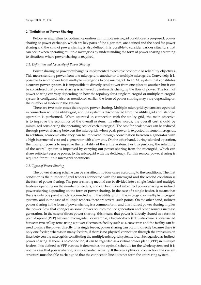
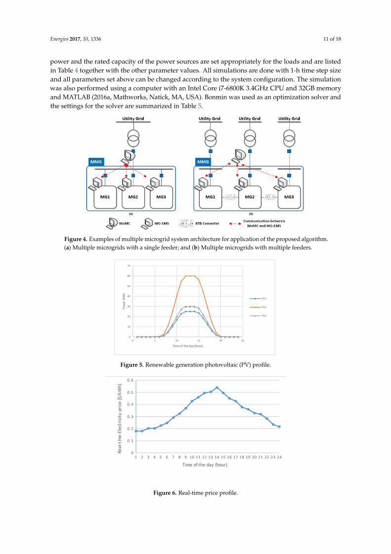
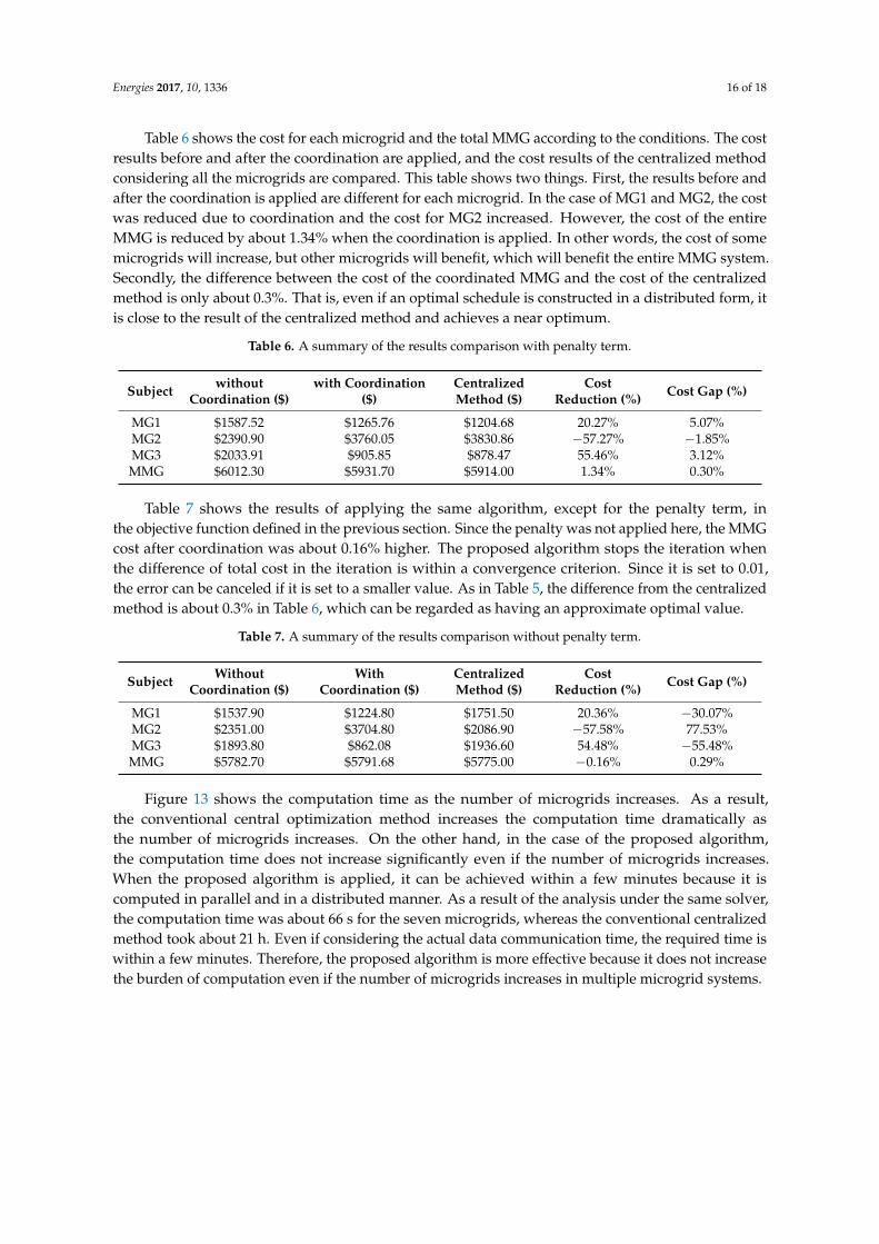
In this section, algorithm verification is performed on multiple microgrids. The multiple microgridsystem can be assumed to have a system structure with a PCC as shown in Figure 4a, or a systemstructure with multiple feeders as shown in Figure 4b. In the case of multiple feeder systemslike Figure 4b, there must be a separate line for power sharing. In this case, the connectionsbetween the microgrids must be electrically isolated through the power electronics in order toprevent the problem of system stability, such as protection cooperation according to the ring topology.The number of the microgrid set is three, to verify the basic performance of the algorithm. As mentionedearlier, each microgrid has only renewable energy sources and battery energy storage systems becausethe microgrid that does have the units without the cost function is focused. For simplicity of analysis,each microgrid was assumed to have one photovoltaic (PV) generation and one battery energy storagesystem (BESS). The PV curve of each microgrid is shown in Figure 5. The system price parameteris based on PJM market data [21], and Figure 6 shows the price curve. The load curves are shownin Figure 7 and the load capacities are summarized in Table 4. The parameters such as the rated output

Energies 2017, 10, 1336 11 of 18

power and the rated capacity of the power sources are set appropriately for the loads and are listedin Table 4 together with the other parameter values. All simulations are done with 1-h time step sizeand all parameters set above can be changed according to the system configuration. The simulationwas also performed using a computer with an Intel Core i7-6800K 3.4GHz CPU and 32GB memoryand MATLAB (2016a, Mathworks, Natick, MA, USA). Bonmin was used as an optimization solver andthe settings for the solver are summarized in Table 5.

Energies 2017, 10, 1336 11 of 19

problem of system stability, such as protection cooperation according to the ring topology. The number of the microgrid set is three, to verify the basic performance of the algorithm. As mentioned earlier, each microgrid has only renewable energy sources and battery energy storage systems because the microgrid that does have the units without the cost function is focused. For simplicity of analysis, each microgrid was assumed to have one photovoltaic (PV) generation and one battery energy storage system (BESS). The PV curve of each microgrid is shown in Figure 5. The system price parameter is based on PJM market data [21], and Figure 6 shows the price curve. The load curves are shown in Figure 7 and the load capacities are summarized in Table 4. The parameters such as the rated output power and the rated capacity of the power sources are set appropriately for the loads and are listed in Table 4 together with the other parameter values. All simulations are done with 1-h time step size and all parameters set above can be changed according to the system configuration. The simulation was also performed using a computer with an Intel Core i7-6800K 3.4GHz CPU and 32GB memory and MATLAB (2016a, Mathworks, Natick, MA, USA). Bonmin was used as an optimization solver and the settings for the solver are summarized in Table 5.

Figure 4. Examples of multiple microgrid system architecture for application of the proposed algorithm. (a) Multiple microgrids with a single feeder; and (b) Multiple microgrids with multiple feeders.

Figure 5. Renewable generation photovoltaic (PV) profile.

0

10

20

30

40

50

60

70

0 5 10 15 20 25

Pow

er [k

W]

Time of the day [hour]

PV1

PV2

PV3

Figure 4. Examples of multiple microgrid system architecture for application of the proposed algorithm.(a) Multiple microgrids with a single feeder; and (b) Multiple microgrids with multiple feeders.

Energies 2017, 10, 1336 11 of 19

problem of system stability, such as protection cooperation according to the ring topology. The number of the microgrid set is three, to verify the basic performance of the algorithm. As mentioned earlier, each microgrid has only renewable energy sources and battery energy storage systems because the microgrid that does have the units without the cost function is focused. For simplicity of analysis, each microgrid was assumed to have one photovoltaic (PV) generation and one battery energy storage system (BESS). The PV curve of each microgrid is shown in Figure 5. The system price parameter is based on PJM market data [21], and Figure 6 shows the price curve. The load curves are shown in Figure 7 and the load capacities are summarized in Table 4. The parameters such as the rated output power and the rated capacity of the power sources are set appropriately for the loads and are listed in Table 4 together with the other parameter values. All simulations are done with 1-h time step size and all parameters set above can be changed according to the system configuration. The simulation was also performed using a computer with an Intel Core i7-6800K 3.4GHz CPU and 32GB memory and MATLAB (2016a, Mathworks, Natick, MA, USA). Bonmin was used as an optimization solver and the settings for the solver are summarized in Table 5.

Figure 4. Examples of multiple microgrid system architecture for application of the proposed algorithm. (a) Multiple microgrids with a single feeder; and (b) Multiple microgrids with multiple feeders.

Figure 5. Renewable generation photovoltaic (PV) profile.

0

10

20

30

40

50

60

70

0 5 10 15 20 25

Pow

er [k

W]


PV1

PV2

PV3

Figure 5. Renewable generation photovoltaic (PV) profile.Energies 2017, 10, 1336 12 of 19

Figure 6. Real-time price profile.

1 2 3 4 5 6 7 8 9 10 11 12 13 14 15 16 17 18 19 20 21 22 23 240

50100150200250300350400450

MG1 MG2 MG3


Pow

er [k

W]

Figure 7. Load profiles of each microgrid.

Table 4. Parameter setting of each microgrid.

Parameter (Unit) MG1 MG2 MG3 Peak Load (kW) 300 500 350

Rated Power of PV (kW) 25 60 30 Rated Output of battery energy storage system (BESS) (kW) 180 500 270

Capacity of BESS (kWh) 180 2000 540 Efficiency of BESS (%) 95 97 96

Upper limit of BESS output (kW) 180 500 270 Lower limit of BESS output (kW) 0 0 0

Upper limit of BESS f (p.u.) 0.9 0.9 0.9 Lower limit of BESS state-of-charge (SOC) (p.u.) 0.2 0.2 0.2

Initial and end SOC of BESS (p.u.) 0.5 0.4 0.4 Predefined Power Limit Value (kW) 245 550 200

Penalty Cost Coefficient 10 10 10 Scale factor 81.67 183.33 100

Time step (h) 1 1 1 The Number of Microgrids (N + M) 3

Convergence Criterion 0.01

1 2 3 4 5 6 7 8 9 10 11 12 13 14 15 16 17 18 19 20 21 22 23 240

0.1

0.2

0.3

0.4

0.5

0.6

Time of the day (hour)

Real

-tim

e El

ectr

icity

pric

e [$

/kW

h]


Energies 2017, 10, 1336 12 of 18

Energies 2017, 10, 1336 12 of 19


1 2 3 4 5 6 7 8 9 10 11 12 13 14 15 16 17 18 19 20 21 22 23 240

50100150200250300350400450

MG1 MG2 MG3


Pow

er [k

W]



Parameter (Unit) MG1 MG2 MG3 Peak Load (kW) 300 500 350

Rated Power of PV (kW) 25 60 30 Rated Output of battery energy storage system (BESS) (kW) 180 500 270

Capacity of BESS (kWh) 180 2000 540 Efficiency of BESS (%) 95 97 96

Upper limit of BESS output (kW) 180 500 270 Lower limit of BESS output (kW) 0 0 0

Upper limit of BESS f (p.u.) 0.9 0.9 0.9 Lower limit of BESS state-of-charge (SOC) (p.u.) 0.2 0.2 0.2

Initial and end SOC of BESS (p.u.) 0.5 0.4 0.4 Predefined Power Limit Value (kW) 245 550 200

Penalty Cost Coefficient 10 10 10 Scale factor 81.67 183.33 100

Time step (h) 1 1 1 The Number of Microgrids (N + M) 3


1 2 3 4 5 6 7 8 9 10 11 12 13 14 15 16 17 18 19 20 21 22 23 240

0.1

0.2

0.3

0.4

0.5

0.6

Time of the day (hour)

Real

-tim

e El

ectr

icity

pric

e [$

/kW

h]



Parameter (Unit) MG1 MG2 MG3

Peak Load (kW) 300 500 350Rated Power of PV (kW) 25 60 30

Rated Output of battery energy storage system (BESS) (kW) 180 500 270Capacity of BESS (kWh) 180 2000 540Efficiency of BESS (%) 95 97 96

Upper limit of BESS output (kW) 180 500 270Lower limit of BESS output (kW) 0 0 0

Upper limit of BESS f (p.u.) 0.9 0.9 0.9Lower limit of BESS state-of-charge (SOC) (p.u.) 0.2 0.2 0.2

Initial and end SOC of BESS (p.u.) 0.5 0.4 0.4Predefined Power Limit Value (kW) 245 550 200

Penalty Cost Coefficient 10 10 10Scale factor 81.67 183.33 100

Time step (h) 1 1 1The Number of Microgrids (N + M) 3


Table 5. Parameter settings for the solver.

Parameter Description Values

Maxiter The number of maximum iteration 1500Maxfeval The number of maximum function evaluation 10,000Maxnodes The number of maximum nodes for the mixed integer solver 10,000Maxtime The number of maximum execution time of the solver 1000Tolrfun The desired relative convergence tolerance of the solver 1.0 × 10−7

Tolafun The desired absolute convergence tolerance of the solver 1.0 × 10−7

Tolint The absolute tolerance used to define whether a solution is an integer value 1.0 × 10−5

Figure 8 shows the daily schedule results of the power supplied from the utility grid for eachmicrogrid. The solid bars are the results before the coordination are applied, the shaded bars showthe results of the coordination applied, and the dotted line is the predetermined limit value for eachmicrogrid. In the figure of the schedule without the coordination, in the case of MG1, the schedule isconfigured to be smaller than the limit value at all times, and only the amount of the power transactionwith utility grid at 1:00, 2:00, and 24:00 are exceeded the limits in MG2, and the limit was exceeded inmost of the times except for 12:00 to 15:00 in MG3. This result shows that MG1 has some margin in alltimes until the limit is exceeded and MG2 has a margin in most time periods, including peak time, and

Energies 2017, 10, 1336 13 of 18

MG3 needs the power sharing from other MGs in the majority of the times. In other words, since MG3pays a penalty for exceeding the limit, it has a cost loss. The expected losses are resolved somewhatthrough power sharing between the microgrids, as shown in Figure 8 (shaded bars). Since eachmicrogrid determines the schedule in consideration of the price curve of the utility system, the result ofthe coordination in MoMC can be interpreted as follows. (1) Net-demand is small in most of the timeincluding peak time, so that MG2, which has enough margin from the limit, changes the scheduleand shares some or all of the power supplied from 3:00 to 23:00 to other MGs as power sharing;(2) in the case of MG1, it is supplied from the grid at the lowest price of 24:00, 1:00, and 2:00, and isshared with other MGs; (3) in case of MG3, since it exceeds the limit in most of the time, it does notpay the penalty cost at all times except 24:00, 1:00, and 2:00 through power shared from MG1 andMG2. Figure 9 shows the state of power sharing by time for each microgrid. Each microgrid constructsa schedule according to its own limit line and calculates a value for power sharing by varying itsschedule according to coordination from the MoMC, and performs power sharing according to thesevalues. When the schedule is changed through coordination, the schedule of the ESSs belonging toeach microgrid also changes. Figures 10 and 11 show the change of SOC and the output of each ESS.

Energies 2017, 10, 1336 13 of 19

Table 5. Parameter settings for the solver.

Parameter Description Values Maxiter The number of maximum iteration 1500

Maxfeval The number of maximum function evaluation 10,000 Maxnodes The number of maximum nodes for the mixed integer solver 10,000 Maxtime The number of maximum execution time of the solver 1000 Tolrfun The desired relative convergence tolerance of the solver 1.0 × 10−7 Tolafun The desired absolute convergence tolerance of the solver 1.0 × 10−7 Tolint The absolute tolerance used to define whether a solution is an integer value 1.0 × 10−5

Figure 8 shows the daily schedule results of the power supplied from the utility grid for each microgrid. The solid bars are the results before the coordination are applied, the shaded bars show the results of the coordination applied, and the dotted line is the predetermined limit value for each microgrid. In the figure of the schedule without the coordination, in the case of MG1, the schedule is configured to be smaller than the limit value at all times, and only the amount of the power transaction with utility grid at 1:00, 2:00, and 24:00 are exceeded the limits in MG2, and the limit was exceeded in most of the times except for 12:00 to 15:00 in MG3. This result shows that MG1 has some margin in all times until the limit is exceeded and MG2 has a margin in most time periods, including peak time, and MG3 needs the power sharing from other MGs in the majority of the times. In other words, since MG3 pays a penalty for exceeding the limit, it has a cost loss. The expected losses are resolved somewhat through power sharing between the microgrids, as shown in Figure 8 (shaded bars). Since each microgrid determines the schedule in consideration of the price curve of the utility system, the result of the coordination in MoMC can be interpreted as follows. (1) Net-demand is small in most of the time including peak time, so that MG2, which has enough margin from the limit, changes the schedule and shares some or all of the power supplied from 3:00 to 23:00 to other MGs as power sharing; (2) in the case of MG1, it is supplied from the grid at the lowest price of 24:00, 1:00, and 2:00, and is shared with other MGs; (3) in case of MG3, since it exceeds the limit in most of the time, it does not pay the penalty cost at all times except 24:00, 1:00, and 2:00 through power shared from MG1 and MG2. Figure 9 shows the state of power sharing by time for each microgrid. Each microgrid constructs a schedule according to its own limit line and calculates a value for power sharing by varying its schedule according to coordination from the MoMC, and performs power sharing according to these values. When the schedule is changed through coordination, the schedule of the ESSs belonging to each microgrid also changes. Figures 10 and 11 show the change of SOC and the output of each ESS.

(a) (b)

0

50

100

150

200

250

300

350

1 2 3 4 5 6 7 8 9 101112131415161718192021222324

Pow

er tr

ansa

ctio

n w

ith U

tility

Grid

[kW

]


Without Coordination With Coordination Limit

0100200300400500600700800

1 2 3 4 5 6 7 8 9 101112131415161718192021222324

Pow

er tr

ansa

ctio

n w

ith U

tility

Grid

[kW

]



Energies 2017, 10, 1336 14 of 19

(c)

Figure 8. Power transaction with utility grid (a) MG1, (b) MG2, (c) MG3.

(a) (b)

(c)

Figure 9. The amount of the power sharing in each microgrid (a) MG1, (b) MG2, (c) MG3.

(a) (b)

050

100150200250300350400

1 2 3 4 5 6 7 8 9 101112131415161718192021222324

Pow

er tr

ansa

ctio

n w

ith U

tility

Grid

[kW

]



-300

-200

-100

0

100

200

300

1 2 3 4 5 6 7 8 9 101112131415161718192021222324

The

amou

nt o

f the

Pow

er S

harin

g[kW

]


Sharing (Send) Sharing (Receive)

-300

-200

-100

0

100

200

300

400

500

1 2 3 4 5 6 7 8 9 101112131415161718192021222324

The

amou

nt o

f the

Pow

er S

harin

g[kW

]



-250

-200

-150

-100

-50

01 2 3 4 5 6 7 8 9 101112131415161718192021222324

The

amou

nt o

f the

Pow

er S

harin

g[kW

]



0

0.2

0.4

0.6

0.8

1

1 2 3 4 5 6 7 8 9 10111213141516171819202122232425

Batt

ery

SOC

[P.U

]


Without Coordination With Coordination

0

0.2

0.4

0.6

0.8

1

1 2 3 4 5 6 7 8 9 10111213141516171819202122232425

Batt

ery

SOC

[P.U

]




Energies 2017, 10, 1336 14 of 18

Energies 2017, 10, 1336 14 of 19

(c)


(a) (b)

(c)


(a) (b)

050

100150200250300350400

1 2 3 4 5 6 7 8 9 101112131415161718192021222324

Pow

er tr

ansa

ctio

n w

ith U

tility

Grid

[kW

]



-300

-200

-100

0

100

200

300

1 2 3 4 5 6 7 8 9 101112131415161718192021222324

The

amou

nt o

f the

Pow

er S

harin

g[kW

]



-300

-200

-100

0

100

200

300

400

500

1 2 3 4 5 6 7 8 9 101112131415161718192021222324

The

amou

nt o

f the

Pow

er S

harin

g[kW

]



-250

-200

-150

-100

-50

01 2 3 4 5 6 7 8 9 101112131415161718192021222324

The

amou

nt o

f the

Pow

er S

harin

g[kW

]



0

0.2

0.4

0.6

0.8

1

1 2 3 4 5 6 7 8 9 10111213141516171819202122232425

Batt

ery

SOC

[P.U

]



0

0.2

0.4

0.6

0.8

1

1 2 3 4 5 6 7 8 9 10111213141516171819202122232425

Batt

ery

SOC

[P.U

]




Energies 2017, 10, 1336 14 of 19

(c)


(a) (b)

(c)


(a) (b)

050

100150200250300350400

1 2 3 4 5 6 7 8 9 101112131415161718192021222324

Pow

er tr

ansa

ctio

n w

ith U

tility

Grid

[kW

]



-300

-200

-100

0

100

200

300

1 2 3 4 5 6 7 8 9 101112131415161718192021222324

The

amou

nt o

f the

Pow

er S

harin

g[kW

]



-300

-200

-100

0

100

200

300

400

500

1 2 3 4 5 6 7 8 9 101112131415161718192021222324

The

amou

nt o

f the

Pow

er S

harin

g[kW

]



-250

-200

-150

-100

-50

01 2 3 4 5 6 7 8 9 101112131415161718192021222324

The

amou

nt o

f the

Pow

er S

harin

g[kW

]



0

0.2

0.4

0.6

0.8

1

1 2 3 4 5 6 7 8 9 10111213141516171819202122232425

Batt

ery

SOC

[P.U

]



0

0.2

0.4

0.6

0.8

1

1 2 3 4 5 6 7 8 9 10111213141516171819202122232425

Batt

ery

SOC

[P.U

]



Energies 2017, 10, 1336 15 of 19

(c)

Figure 10. Battery SOC in each microgrid (a) MG1, (b) MG2, (c) MG3.

(a) (b)

(c)

Figure 11. Battery output in each microgrid (a) MG1, (b) MG2, (c) MG3.

The change in the schedule of each microgrid through this coordination is due to the change of the net-demand shown in Figure 12. The MoMC calculates the amount of the power sharing and reflects these values to the net-demand of each MG; it delivers the coordinated net-demand to each MG-EMS, and then the MG-EMS uses the coordinated net-demand to change its own schedule. Therefore, the amount of the power sharing shown in Figure 9 reflects the change of the power schedule supplied from the utility grid and the change of the ESS schedule.

0

0.2

0.4

0.6

0.8

1

1 2 3 4 5 6 7 8 9 10111213141516171819202122232425

Batt

ery

SOC

[P.U

]



-140-120-100-80-60-40-20020406080

1 2 3 4 5 6 7 8 9 101112131415161718192021222324

Out

put P

ower

[kW

]



-600

-400

-200

0

200

400

600

1 2 3 4 5 6 7 8 9 101112131415161718192021222324

Out

put P

ower

[kW

]



-250-200-150-100-500

50100150

1 2 3 4 5 6 7 8 9 101112131415161718192021222324

Out

put P

ower

[kW

]




Energies 2017, 10, 1336 15 of 18

Energies 2017, 10, 1336 15 of 19

(c)


(a) (b)

(c)


The change in the schedule of each microgrid through this coordination is due to the change of the net-demand shown in Figure 12. The MoMC calculates the amount of the power sharing and reflects these values to the net-demand of each MG; it delivers the coordinated net-demand to each MG-EMS, and then the MG-EMS uses the coordinated net-demand to change its own schedule. Therefore, the amount of the power sharing shown in Figure 9 reflects the change of the power schedule supplied from the utility grid and the change of the ESS schedule.

0

0.2

0.4

0.6

0.8

1

1 2 3 4 5 6 7 8 9 10111213141516171819202122232425

Batt

ery

SOC

[P.U

]



-140-120-100-80-60-40-20020406080

1 2 3 4 5 6 7 8 9 101112131415161718192021222324

Out

put P

ower

[kW

]



-600

-400

-200

0

200

400

600

1 2 3 4 5 6 7 8 9 101112131415161718192021222324

Out

put P

ower

[kW

]



-250-200-150-100-500

50100150

1 2 3 4 5 6 7 8 9 101112131415161718192021222324

Out

put P

ower

[kW

]




The change in the schedule of each microgrid through this coordination is due to the changeof the net-demand shown in Figure 12. The MoMC calculates the amount of the power sharingand reflects these values to the net-demand of each MG; it delivers the coordinated net-demand toeach MG-EMS, and then the MG-EMS uses the coordinated net-demand to change its own schedule.Therefore, the amount of the power sharing shown in Figure 9 reflects the change of the power schedulesupplied from the utility grid and the change of the ESS schedule.Energies 2017, 10, 1336 16 of 19

(a) (b)

(c)

Figure 12. Changes in net-demand for each microgrid (a) MG1, (b) MG2, (c) MG3.

Table 6 shows the cost for each microgrid and the total MMG according to the conditions. The cost results before and after the coordination are applied, and the cost results of the centralized method considering all the microgrids are compared. This table shows two things. First, the results before and after the coordination is applied are different for each microgrid. In the case of MG1 and MG2, the cost was reduced due to coordination and the cost for MG2 increased. However, the cost of the entire MMG is reduced by about 1.34% when the coordination is applied. In other words, the cost of some microgrids will increase, but other microgrids will benefit, which will benefit the entire MMG system. Secondly, the difference between the cost of the coordinated MMG and the cost of the centralized method is only about 0.3%. That is, even if an optimal schedule is constructed in a distributed form, it is close to the result of the centralized method and achieves a near optimum.

Table 6. A summary of the results comparison with penalty term.

Subject without Coordination ($)

with Coordination ($)

Centralized Method ($)

Cost Reduction (%) Cost Gap (%) MG1 $1587.52 $1265.76 $1204.68 20.27% 5.07%MG2 $2390.90 $3760.05 $3830.86 −57.27% −1.85%MG3 $2033.91 $905.85 $878.47 55.46% 3.12%MMG $6012.30 $5931.70 $5914.00 1.34% 0.30%

Table 7 shows the results of applying the same algorithm, except for the penalty term, in the objective function defined in the previous section. Since the penalty was not applied here, the MMG cost after coordination was about 0.16% higher. The proposed algorithm stops the iteration when the difference of total cost in the iteration is within a convergence criterion. Since it is set to 0.01, the error can be canceled if it is set to a smaller value. As in Table 5, the difference from the centralized method is about 0.3% in Table 6, which can be regarded as having an approximate optimal value.

050100150200250300350

1 2 3 4 5 6 7 8 9 101112131415161718192021222324

Net

Dem

and

[kW

]


Original Net Demand Coordinated Net Demand

0100200300400500600700800

1 2 3 4 5 6 7 8 9 101112131415161718192021222324

Net

Dem

and

[kW

]



0

50

100

150

200

250

300

1 2 3 4 5 6 7 8 9 101112131415161718192021222324

Net

Dem

and

[kW

]



Figure 12. Changes in net-demand for each microgrid (a) MG1, (b) MG2, (c) MG3.

Energies 2017, 10, 1336 16 of 18

Table 6 shows the cost for each microgrid and the total MMG according to the conditions. The costresults before and after the coordination are applied, and the cost results of the centralized methodconsidering all the microgrids are compared. This table shows two things. First, the results before andafter the coordination is applied are different for each microgrid. In the case of MG1 and MG2, the costwas reduced due to coordination and the cost for MG2 increased. However, the cost of the entireMMG is reduced by about 1.34% when the coordination is applied. In other words, the cost of somemicrogrids will increase, but other microgrids will benefit, which will benefit the entire MMG system.Secondly, the difference between the cost of the coordinated MMG and the cost of the centralizedmethod is only about 0.3%. That is, even if an optimal schedule is constructed in a distributed form, itis close to the result of the centralized method and achieves a near optimum.

Table 6. A summary of the results comparison with penalty term.

Subject withoutCoordination ($)

with Coordination($)

CentralizedMethod ($)

CostReduction (%) Cost Gap (%)

MG1 $1587.52 $1265.76 $1204.68 20.27% 5.07%MG2 $2390.90 $3760.05 $3830.86 −57.27% −1.85%MG3 $2033.91 $905.85 $878.47 55.46% 3.12%MMG $6012.30 $5931.70 $5914.00 1.34% 0.30%

Table 7 shows the results of applying the same algorithm, except for the penalty term, inthe objective function defined in the previous section. Since the penalty was not applied here, the MMGcost after coordination was about 0.16% higher. The proposed algorithm stops the iteration whenthe difference of total cost in the iteration is within a convergence criterion. Since it is set to 0.01,the error can be canceled if it is set to a smaller value. As in Table 5, the difference from the centralizedmethod is about 0.3% in Table 6, which can be regarded as having an approximate optimal value.

Table 7. A summary of the results comparison without penalty term.

Subject WithoutCoordination ($)

WithCoordination ($)

CentralizedMethod ($)

CostReduction (%) Cost Gap (%)

MG1 $1537.90 $1224.80 $1751.50 20.36% −30.07%MG2 $2351.00 $3704.80 $2086.90 −57.58% 77.53%MG3 $1893.80 $862.08 $1936.60 54.48% −55.48%MMG $5782.70 $5791.68 $5775.00 −0.16% 0.29%

Figure 13 shows the computation time as the number of microgrids increases. As a result,the conventional central optimization method increases the computation time dramatically asthe number of microgrids increases. On the other hand, in the case of the proposed algorithm,the computation time does not increase significantly even if the number of microgrids increases.When the proposed algorithm is applied, it can be achieved within a few minutes because it iscomputed in parallel and in a distributed manner. As a result of the analysis under the same solver,the computation time was about 66 s for the seven microgrids, whereas the conventional centralizedmethod took about 21 h. Even if considering the actual data communication time, the required time iswithin a few minutes. Therefore, the proposed algorithm is more effective because it does not increasethe burden of computation even if the number of microgrids increases in multiple microgrid systems.

Energies 2017, 10, 1336 17 of 18

Energies 2017, 10, 1336 17 of 19

Table 7. A summary of the results comparison without penalty term.

Subject Without Coordination ($)

With Coordination ($)

Centralized Method ($)

Cost Reduction (%) Cost Gap (%)

MG1 $1537.90 $1224.80 $1751.50 20.36% −30.07% MG2 $2351.00 $3704.80 $2086.90 −57.58% 77.53% MG3 $1893.80 $862.08 $1936.60 54.48% −55.48% MMG $5782.70 $5791.68 $5775.00 −0.16% 0.29%

Figure 13 shows the computation time as the number of microgrids increases. As a result, the conventional central optimization method increases the computation time dramatically as the number of microgrids increases. On the other hand, in the case of the proposed algorithm, the computation time does not increase significantly even if the number of microgrids increases. When the proposed algorithm is applied, it can be achieved within a few minutes because it is computed in parallel and in a distributed manner. As a result of the analysis under the same solver, the computation time was about 66 s for the seven microgrids, whereas the conventional centralized method took about 21 h. Even if considering the actual data communication time, the required time is within a few minutes. Therefore, the proposed algorithm is more effective because it does not increase the burden of computation even if the number of microgrids increases in multiple microgrid systems.

Figure 13. Computation time according to the number of microgrids using centralized method.

6. Conclusions

In this paper, a distributed coordination strategy is proposed between microgrids for the optimal operation of the whole system under a hierarchical multiple microgrid system. The optimal operation of the entire microgrid system is achieved through the determination of individual schedules in each microgrid and the iterative execution of coordination is performed in terms of the overall system. The proposed algorithm is verified by simulation using MATLAB. As a result of the simulation, it is shown that the total cost has been reduced by paying less penalty cost after coordination at MoMC. Compared with the results of applying the centralized method, the difference between the total cost of the proposed algorithm and that of the centralized method is less than 1%, regardless of the penalty term of the objective function of each microgrid. This means that the proposed power sharing algorithm through the coordination is valid without a special penalty cost function, which is practical in multiple microgrids consisting of only ESSs or renewable energy resources without an energy cost function. Finally, comparing the computation time with the increase of the number of microgrids shows that the proposed algorithm has a considerable advantage in terms of computational burden and time required. Therefore, this algorithm can be applied not only to determine the day-ahead schedule but also to determine the real-time schedule. In summary, the advantages of the proposed algorithm are as follows: (1) it is a power sharing strategy of multiple microgrids considering multiple

0

200

400

600

800

1000

1200

1400

1 3 5 7

Com

puta

tiona

l tim

e [m

in]

The number of MG

Centralized method Proposed algorithm

Figure 13. Computation time according to the number of microgrids using centralized method.

6. Conclusions

In this paper, a distributed coordination strategy is proposed between microgrids for the optimaloperation of the whole system under a hierarchical multiple microgrid system. The optimal operationof the entire microgrid system is achieved through the determination of individual schedules in eachmicrogrid and the iterative execution of coordination is performed in terms of the overall system.The proposed algorithm is verified by simulation using MATLAB. As a result of the simulation, it isshown that the total cost has been reduced by paying less penalty cost after coordination at MoMC.Compared with the results of applying the centralized method, the difference between the total cost ofthe proposed algorithm and that of the centralized method is less than 1%, regardless of the penaltyterm of the objective function of each microgrid. This means that the proposed power sharing algorithmthrough the coordination is valid without a special penalty cost function, which is practical in multiplemicrogrids consisting of only ESSs or renewable energy resources without an energy cost function.Finally, comparing the computation time with the increase of the number of microgrids shows thatthe proposed algorithm has a considerable advantage in terms of computational burden and timerequired. Therefore, this algorithm can be applied not only to determine the day-ahead schedule butalso to determine the real-time schedule. In summary, the advantages of the proposed algorithm are asfollows: (1) it is a power sharing strategy of multiple microgrids considering multiple feeder structuresas well as a single feeder structure for minimizing the operation cost of the entire system; (2) it isa power sharing strategy between microgrids that can be applied in a microgrid where only units thatdo not have a cost function exist; (3) since it is the optimization of the distributed form, the computationtime decreases sharply compared with the one performed at the central center. In future works, wewill study the operational strategy of improving the economics through power sharing for peak powercontrol when constructing real-time schedules.

Acknowledgments: This work was supported by the Korea Institute of Energy Technology Evaluation andPlanning (KETEP) and the Ministry of Trade, Industry & Energy (MOTIE) of the Korea (No. 20151210200080).This research was supported by Basic Science Research Program through the National Research Foundation ofKorea (NRF), funded by the Ministry of Education, Science and Technology (Grant no. NRF-2013R1A1A1012667).

Author Contributions: Won-Poong Lee carried out the main research tasks and wrote the full manuscript, andJin-Young Choi provided technical support to verify the proposed algorithm in simulation software. Dong-Jun Wonvalidated and double-checked the proposed algorithm, the results, and the whole manuscript.

Conflicts of Interest: The authors declare no conflict of interest.

References

1. Olivares, D.E.; Mehrizi-Sani, A.; Etemadi, A.H.; Canizares, C.A.; Iravani, R.; Kazerani, M.; Hajimiragha, A.H.;Gomis-Bellmunt, O.; Saeedifard, M.; Palma-Behnke, R.; et al. Trends in microgrid control. IEEE Trans.Smart Grid 2014, 5, 1905–1919. [CrossRef]

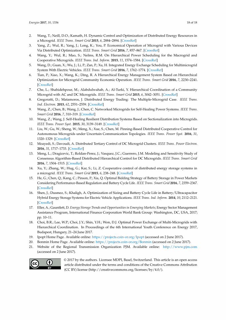
http://dx.doi.org/10.1109/TSG.2013.2295514

Energies 2017, 10, 1336 18 of 18

2. Wang, T.; Neill, D.O.; Kamath, H. Dynamic Control and Optimization of Distributed Energy Resources ina Microgrid. IEEE Trans. Smart Grid 2015, 6, 2884–2894. [CrossRef]

3. Yang, Z.; Wul, R.; Yang, J.; Long, K.; You, P. Economical Operation of Microgrid with Various DevicesVia Distributed Optimization. IEEE Trans. Smart Grid 2016, 7, 857–867. [CrossRef]

4. Wang, Y.; Wul, R.; Mao, S.; Nelms, R.M. On Hierarchical Power Scheduling for the Macrogrid andCooperative Microgrids. IEEE Trans. Ind. Inform. 2015, 11, 1574–1584. [CrossRef]

5. Wang, D.; Guan, X.; Wu, J.; Li, P.; Zan, P.; Xu, H. Integrated Energy Exchange Scheduling for MultimicrogridSystem With Electric Vehicles. IEEE Trans. Smart Grid 2016, 7, 1762–1774. [CrossRef]

6. Tian, P.; Xiao, X.; Wang, K.; Ding, R. A Hierarchical Energy Management System Based on HierarchicalOptimization for Microgrid Community Economic Operation. IEEE Trans. Smart Grid 2016, 7, 2230–2241.[CrossRef]

7. Che, L.; Shahidehpour, M.; Alabdulwahab, A.; Al-Turki, Y. Hierarchical Coordination of a CommunityMicrogrid with AC and DC Microgrids. IEEE Trans. Smart Grid 2015, 6, 3042–3051. [CrossRef]

8. Gregoratti, D.; Matamoros, J. Distributed Energy Trading: The Multiple-Microgrid Case. IEEE Trans.Ind. Electron. 2015, 62, 2551–2559. [CrossRef]

9. Wang, Z.; Chen, B.; Wang, J.; Chen, C. Networked Microgrids for Self-Healing Power Systems. IEEE Trans.Smart Grid 2016, 7, 310–319. [CrossRef]

10. Wang, Z.; Wang, J. Self-Healing Resilient Distribution Systems Based on Sectionalization into Microgrids.IEEE Trans. Power Syst. 2015, 30, 3139–3149. [CrossRef]

11. Liu, W.; Gu, W.; Sheng, W.; Meng, X.; Xue, S.; Chen, M. Pinning-Based Distributed Cooperative Control forAutonomous Microgrids under Uncertain Communication Topologies. IEEE Trans. Power Syst. 2016, 31,1320–1329. [CrossRef]

12. Moayedi, S.; Davoudi, A. Distributed Tertiary Control of DC Microgrid Clusters. IEEE Trans. Power Electron.2016, 31, 1717–1733. [CrossRef]

13. Meng, L.; Dragicevic, T.; Roldan-Perez, J.; Vasquez, J.C.; Guerrero, J.M. Modeling and Sensitivity Study ofConsensus Algorithm-Based Distributed Hierarchical Control for DC Microgrids. IEEE Trans. Smart Grid2016, 7, 1504–1515. [CrossRef]

14. Xu, Y.; Zhang, W.; Hug, G.; Kar, S.; Li, Z. Cooperative control of distributed energy storage systems ina microgrid. IEEE Trans. Smart Grid 2015, 6, 238–248. [CrossRef]

15. He, G.; Chen, Q.; Kang, C.; Pinson, P.; Xia, Q. Optimal Bidding Strategy of Battery Storage in Power MarketsConsidering Performance-Based Regulation and Battery Cycle Life. IEEE Trans. Smart Grid 2016, 7, 2359–2367.[CrossRef]

16. Shen, J.; Dusmez, S.; Khaligh, A. Optimization of Sizing and Battery Cycle Life in Battery/UltracapacitorHybrid Energy Storage Systems for Electric Vehicle Applications. IEEE Trans. Ind. Inform. 2014, 10, 2112–2121.[CrossRef]

17. Eller, A.; Gauntlett, D. Energy Storage Trends and Opportunities in Emerging Markets; Energy Sector ManagementAssistance Program, International Finance Corporation World Bank Group: Washington, DC, USA, 2017;pp. 10–11.

18. Choi, B.R.; Lee, W.P.; Choi, J.Y.; Shin, Y.H.; Won, D.J. Optimal Power Exchange of Multi-Microgrids withHierarchical Coordination. In Proceedings of the 6th International Youth Conference on Energy 2017,Budapest, Hungary, 21–24 June 2017.

19. Ipopt Home Page. Available online: https://projects.coin-or.org/Ipopt (accessed on 2 June 2017).20. Bonmin Home Page. Available online: https://projects.coin-or.org/Bonmin (accessed on 2 June 2017).21. Website of the Regional Transmission Organization PJM. Available online: http://www.pjm.com

(accessed on 2 June 2017).

© 2017 by the authors. Licensee MDPI, Basel, Switzerland. This article is an open accessarticle distributed under the terms and conditions of the Creative Commons Attribution(CC BY) license (http://creativecommons.org/licenses/by/4.0/).



http://dx.doi.org/10.1109/TII.2015.2417496




http://dx.doi.org/10.1109/TIE.2014.2352592


http://dx.doi.org/10.1109/TPWRS.2015.2389753

http://dx.doi.org/10.1109/TPWRS.2015.2421639

http://dx.doi.org/10.1109/TPEL.2015.2424672




http://dx.doi.org/10.1109/TII.2014.2334233

https://projects.coin-or.org/Ipopt

https://projects.coin-or.org/Bonmin

http://www.pjm.com

http://creativecommons.org/

http://creativecommons.org/licenses/by/4.0/.

Documents

Multiple Microgrids Based on Hierarchical System