Embed Size (px)
Citation preview
UNIVERSITY OF PADOVA FACOLTÀ DI INGEGNERIA
PH.D. THESIS
Sede Amministrativa: Università degli Studi di Padova
Dipartimento di Ingegneria dell’informazione
DOTTORATO DI RICERCA IN:
INGEGNERIA ELETTRONICA E DELLE TELECOMUNICAZIONI
CICLO XX
Multiple Description Coding forNon-Scalable and Scalable Video
Compression
Coordinatore: Ch.mo Prof. Silvano Pupolin
Relatori: Ch.mo Prof. Giancarlo Calvagno
Ch.mo Prof. Gian Antonio Mian
Dottorando: Ottavio Campana
Gennaio 2008
CORSO DI LAUREA IN INGEGNERIA
DELLE TELECOMUNICAZIONI
DIPARTIMENTO DI INGEGNERIA
DELL’INFORMAZIONE


to the memory of Gian Antonio Mian


Contents
Summary 1
Sommario 3
1 Introduction 5
1.1 The channel splitting scheme . . . . . . . . . . . . . . . . . . . . 7
1.2 The MD RD region . . . . . . . . . . . . . . . . . . . . . . . . . . 12
1.2.1 The MD RD region for the channel splitting scheme . . . 19
1.2.2 The Redundancy Rate-Distortion Region . . . . . . . . . 21
1.3 Applications to image and video coding . . . . . . . . . . . . . . 22
1.3.1 MD coding with Correlating Transforms . . . . . . . . . 22
1.3.2 MD coding with Frames . . . . . . . . . . . . . . . . . . . 25
1.3.3 MD coding with Motion Compensation . . . . . . . . . . 27
2 H.264/AVC-based MDC schemes 31
2.1 Introduction to H.264/AVC . . . . . . . . . . . . . . . . . . . . . 31
2.1.1 Intra prediction . . . . . . . . . . . . . . . . . . . . . . . . 32
2.1.2 Motion estimation . . . . . . . . . . . . . . . . . . . . . . 33
2.1.3 Integer transform . . . . . . . . . . . . . . . . . . . . . . . 37
2.1.4 Entropy coding . . . . . . . . . . . . . . . . . . . . . . . . 38
2.1.5 In-loop deblocking filter . . . . . . . . . . . . . . . . . . . 39
2.2 Test conditions . . . . . . . . . . . . . . . . . . . . . . . . . . . . . 40
2.3 Sub-Sampling Multiple Description Coding . . . . . . . . . . . . 41
2.4 Multiple Description Motion Coding . . . . . . . . . . . . . . . . 44
2.5 Multiple State Video Coder . . . . . . . . . . . . . . . . . . . . . 50
2.6 Motion-Compensated Multiple Description Video Coding . . . 56
2.7 MDSQ-based Multiple Description Video Coding . . . . . . . . 62
2.7.1 The Multiple Description Scalar Quantizer . . . . . . . . 62
2.7.2 Implementation of the scheme . . . . . . . . . . . . . . . 66
2.8 Performance comparison of the proposed schemes . . . . . . . . 71
i

CONTENTS
2.8.1 Schemes comparison . . . . . . . . . . . . . . . . . . . . . 71
3 Scalable Video Coding 75
3.1 Introduction to Scalable Video Coding . . . . . . . . . . . . . . . 75
3.1.1 Scalability in existing coding standards . . . . . . . . . . 76
3.1.2 Wavelets and wavelet-based spatial scalability . . . . . . 78
3.1.3 SNR scalability for predictive coding techniques . . . . . 84
3.1.4 SNR scalability for non predictive coding techniques . . 87
3.1.5 Temporal scalability techniques . . . . . . . . . . . . . . . 94
3.2 Protection enhanced scalable video coder . . . . . . . . . . . . . 100
3.2.1 Spatial Multiple Description Coding . . . . . . . . . . . . 105
3.2.2 MDSQ-based Multiple Description Coding . . . . . . . . 106
3.2.3 Temporal Multiple Description Coding . . . . . . . . . . 108
3.2.4 Experimental Results . . . . . . . . . . . . . . . . . . . . . 110
3.2.5 Spatial Multiple Description Coding . . . . . . . . . . . . 112
3.2.6 Temporal Multiple Description Coding . . . . . . . . . . 117
3.2.7 Comparison between the spatial and temporal approaches120
4 Conclusions 123
ii

Summary
Multiple Description Coding (MDC) techniques are based on dividing the in-
put signal into several chunks of data called descriptions. Whenever all de-
scriptions are correctly received the original signal is reconstructed, while in
case some information is lost its content is estimated by exploiting the redun-
dancy shared between all the descriptions and a coarse approximation of the
signal is decoded.
Clearly, the main goal of MDC is to provide a method for joint source-
channel coding, but it has a major characteristic that makes it different from
many other techniques. In fact, many joint source-channel coding techniques
rely on joint source channel optimization, thus given the knowledge of the
transmission channel packet error rate they optimize the bitrate allocation in
source and channel coding so that the quality of the decoded sequence is max-
imized. MDC techniques do not require the knowledge of the channel and
the introduced redundancy is chosen starting from the source coding scheme
and not from the channel coding strategy. This duality can be expressed as
thinking that in the first case joint source channel coding is obtained starting
form channel coding and successively jointly perform source coding, while in
MDC attention if first paid to source coding and successively channel coding
is taken into account. This aspect is indeed reflected in the channel agnosia
that characterizes most MDC schemes.
MDC was proposed at the beginning of the 70s for the speech signal and is
has been successively applied to many fields like video coding, data transmis-
sion, data storage and wireless sensors networks. The topic of this thesis is the
application of MDC to non-scalable and scalable video coding.
In the first chapter, an introduction to MDC is given. This is necessary be-
cause basic results in MDC where never published, but they were only written
in Bell Labs internal reports. Thus, accessing the basic theory is practically im-
possible, and most of results are only available in some old papers which not
only reference those reports, but also reference their results. The chapter be-
gins with a review of the first MDC scheme, known as the Jayant scheme and
1

Summary
from its performance analysis the MDC problem is formulated. Successively,
after an introduction to classic Rate-Distortion theory, the MD Rate-Distortion
theory is similarly derived and the Cover and El Gamal theorem is enunciated.
Finally, some MD applications to video coding are presented.
In the second chapter, MDC schemes for the H.264/AVC coding standard
are presented. The main purpose of this chapter is to summarize all the schemes
that have been studied in the Signal and Image Image Processing Laboratory
at University of Padova during the last years, because this research can be
considered concluded. The proposed MDC schemes involve several aspects of
the H.264/AVC encoder, in fact some of them exploit the spatial correlation of
video sequences, others rely on temporal correlation and others work on the
produced bitstream to generate the descriptions.
The third chapter is focused on Scalable Video Coding (SVC) and MDC.
This research was performed while I was visiting the Video Processing Labo-
ratory at University of California, San Diego and was supported in part by a
scholarship from the “Fondazione A. Gini” (Padova, Italy). The proposed SVC
scheme is not related to any existing standard, but it involves motion compen-
sation of wavelet-decomposed frames to provide spatial, temporal and SNR
scalability. The encoder structure is inspired by the Responses of call for proposal
for scalable video coding of W. J. Han. The codec was completely written from
scratch and by implementing the wavelet transform, the temporal prediction
strategies, the bitplane coding algorithms and the MDC schemes. Finally the
schemes performance are presented and the results are compared.
2

Sommario
La Codifica a Descrizioni Multiple si basa sulla divisione del segnale in in-
gresso al sistema di codifica in vari sottoinsiemi di informazioni, detti
descrizioni. Quando tutte le descrizioni sono correttamente ricevute, il deco-
dificatore è in grado di ricostruire il segnale originario, mentre se si verificano
degli errori di trasmissione è possibile sfruttare la ridondanza condivisa tra
tutte le descrizioni per stimare i dati persi e ricostruire una approssimazione
del segnale originale.
Lo scopo principale della codifica a descrizioni multiple consiste nella
trasmissione robusta dell’informazione fornendo delle tecniche di codifica con-
giunta sorgente e canale, ma ha delle peculiarità che le differenziano da molte
altre tecniche di codifica congiunta. Infatti, la maggior parte delle tecniche pro-
poste effettuano una ottimizzazione congiunta e perciò
richiedono la conoscenza della statistica che caratterizza il canale di trasmis-
sione. Conoscendo la statistica del canale è possibile decidere il partiziona-
mento ottimo del bitstream tra la codifica di canale e di sorgente per mas-
simizzare la qualità del segnale ricostruito. Al contrario, le tecniche di codi-
fica a descrizioni multiple non richiedono la conoscenza del canale e la ridon-
danza introdotta dal processo di codifica viene scelta a partire dallo schema di
compressione. Questa dualità può essere spiegata considerando che nel primo
caso la codifica congiunta di sorgente e canale inizia dalla scelta della codifica
di canale per poi ottimizzare la codifica di sorgente, mentre nel secondo caso
per prima cosa viene considerata la compressione del segnale e la codifica di
canale viene considerata successivamente. Questa inversione nell’approccio
alla codifica congiunta si rispecchia nell’agnosia del canale che caratterizza la
maggior parte degli schemi di codifica a descrizioni multiple.
La Codifica a Descrizioni Multiple è stata introdotta agli inizi degli anni
settanta per la trasmissione del segnale vocale ed è stata applicata successiva-
mente ad altri campi, quali ad esempio codifica video, trasmissioni numerica,
archiviazione di dati e reti di sensori wireless. L’argomento di questa tesi è la
Codifica a Descrizioni Multiple applicata alla codifica video scalabile e non.
3

Sommario
Nel primo capitolo viene introdotta la Codifica a Descrizioni Multiple.
Questa introduzione è resa necessaria dalla frammentazione della teoria, che
specialmente all’inizio è stata sviluppata e pubblicata nei report interni dei
Bell Labs e che quindi è difficilmente accessibile. Di conseguenza la mag-
gior parte dei risultati teorici non sono direttamente accessibili, ma possono
essere ritrovati in alcuni articoli che oltre a citare i report interni ne riportano
anche i risultati. Il capitolo inizia con la presentazione del primo schema di
codifica a descrizioni multiple, conosciuto anche come schema di Jayant, e
dall’analisi delle sue prestazioni viene formulato il problema della Codifica
a Descrizioni Multiple. Successivamente, dopo un richiamo alla teoria classica
di Rate-Distortion, la teoria Rate-Distortion per la Codifica a Descrizioni Mul-
tiple viene presentata e viene enunciato il teorema di Cover ed El Gamal. Per
finire sono illustrate alcune applicazioni per la codifica video.
L’argomento del secondo capitolo è costituito dalla codifica video non sca-
labile e dagli schemi sviluppati per lo standard di codifica H.264/AVC. Lo
scopo principale di questo capitolo è di riassumere tutti i risultati della ricerca
sviluppata nel corso degli anni presso il Laboratorio di Elaborazione dei Se-
gnali e delle Immagini dell’Università di Padova e che si può ormai conside-
rare conclusa. Gli schemi proposti coprono aspetti anche distinti del codifica-
tore H.264/AVC, infatti alcuni sfruttano la ridondanza spaziale delle sequenze
video, altri invece si basano sulla ridondanza temporale e altri ancora lavorano
direttamente sul bitstream compresso prodotto dal codificatore.
Per finire il terzo capitolo è rivolto alla Codifica Video Scalabile e alla Co-
difica a Descrizioni Multiple ad essa applicata. Questa ricerca è stata svolta
durante il periodo di scambio all’estero presso il Video Processing Labora-
tory dell’Università della California, San Diego, ed è stata supportata in parte
da una borsa di studio della “Fondazione A.Gini” di Padova. Lo schema di
codifica video scalabile non è basato su alcuno standard, ma sfrutta la moto
compensazione di frame decomposti mediante le wavelet per fornire scala-
bilità spaziale, temporale e in qualità. La struttura del codificatore è stata
ispirata dalla Responses of call for proposal for scalable video coding di W. J. Han.
Il codificatore è stato scritto completamente in C, a partire dalla trasformata
wavelet, la decomposizione per la motocompensazione e gli algoritmi per la
codifica a piani di bit e compressione delle immagini e dei residui. Per finire le
prestazioni dei vari schemi di codifica a descrizioni multiple per il codificatore
vengono presentate e confrontate.
4

Chapter 1
Introduction
The main goal of source coding consists in representing the information with the
minimum number of bits, in order to reduce the required bandwidth. Thus,
more parallel transmissions are feasible, even without any change to the net-
work, which might not be easily done because of technological limits or eco-
nomical constraints.
By reducing the bitstream size and by rising the coding efficiency, the major
drawback quickly becomes visible: compressed data more likely suffers trans-
mission errors than uncompressed information, because errors propagate in
encoded data. As an example, when samples are encoded by using prediction,
a valid reference is indispensable for flawless reconstruction.
In order to guarantee the reconstructed signal quality, several channel coding
techniques were developed. All these techniques add redundancy to enhance
transmission robustness with respect to channel errors.
Even though source and channel coding are dual problems, they have been
considered as separated topics for many years. Video coding standards such
as MPEG-1, MPEG-2, H.263 or the latter H.264/AVC where developed by fo-
cusing only on compression efficiency and by abstracting the transport char-
acteristics, relying on an adaptation layer to properly adapt the compressed
bitstream for transmission or storage. This strategy was mainly supported by
Shannon’s source-channel separation theorem.
Definition 1 Let X be a discrete random variable with alphabet X and probability
mass function p(x) = P{X = x}, x ∈ X . The entropy H(X) of a discrete random
variable X is defined by
H(X) = − ∑x∈X
p(x) log p(x). (1.1)
5
Definition 2 Consider two random variables X and Y with a joint probability mass
function p(x, y) and marginal probability mass functions p(x) and p(y). The mu-
tual information I(X; Y) is the relative entropy between the joint distribution and the
product distribution p(x)p(y):
I(X; Y) = ∑x∈X
∑y∈Y
p(x, y) logp(x, y)
p(x)p(y)(1.2)
Definition 3 A discrete channel is a system consisting of an input alphabet X , an
output channel Y and a probability transition matrix p(y|x) that expresses the proba-
bility of observing the output symbol y given that the symbol y was sent. The channel
is said to be memoryless if the probability distribution of the output depends only on
the input at that time and is conditionally independent of previous channel inputs or
outputs.
Definition 4 The “information” channel capacity of a discrete memoryless channel
is defined as
C = maxp(x)
I(X; Y) , (1.3)
where the maximum is taken over all possible input distributions p(x).
Capacity is bounded to the channel statistic, which can be expressed in
terms of Signal-to-Noise Ratio (SNR). For example, in case of a binary sym-
metric channel, it can be shown that I(X; Y) ≤ 1− H(p), where p is the proba-
bility of transmission error and depends on the adopted modulation and noise
power.
Given these definitions, the Shannon’s source-channel coding theorem can
be stated:
Theorem 1 (Source-channel coding theorem): If X = {X1,X2, · · · ,Xn} is a finite
alphabet stochastic process that satisfies the AEP, then there exists a source channel
code with P(n)e → 0 if H(X ) < C.
Conversely, for any stationary stochastic process, if H(X ) > C, the probability error
is bounded away from zero, and it is not possible to send the process over the channel
with arbitrarily low probability of error.
To guarantee optimality, this theorem requires the channel capacity to be
big enough to hold the compressed bitrate. This reflects in SNRs sufficiently
high to guarantee the needed capacity. The theorem was stated for unicast
channel, but it has been successively extended to the broadcast channel, and
in this case the capacity is in general further reduced. Moreover, the theorem
6
1.1. The channel splitting scheme
result is achieved asymptotically, so it may be possible that a practical joint
source/channel coding techniques are preferable to separate schemes
Multiple Description Coding (MDC) [Goy01a] techniques can be generally
classified as joint source channel coding, even though they do not often con-
sider the channel statistics. In fact, MDC techniques do not require the knowl-
edge of the channel and the introduced redundancy is chosen starting from the
source coding scheme and not from the channel coding strategy. Nevertheless,
they try to enhance transmission robustness by dividing the input signal into
chunks of data called descriptions and by exploiting the channel diversity for
transmission. At the receiver, whenever all the descriptions are correctly re-
ceived, the original signal is reconstructed, while in case of information loss,
the correlation between the descriptions is exploited to estimated the lost in-
formation and to reconstruct an approximation of the original signal.
By dividing the original signals into several descriptions, only suboptimal
compression ratios are achieved, because additional redundancy is introduced.
Fortunately, this additional information is exploited to reconstruct the signal in
case of transmission errors, and has the same role of channel coding when op-
timality is guaranteed by the separation theorem. Therefore, MDC techniques
represent a strategy that can be exploited when the source-channel separation
theorem does not hold or cannot be applied.
1.1 The channel splitting scheme
We do now introduce one of the first known MDC schemes, the channel split-
ting scheme. Due to its simplicity, this scheme is an easily understandable ex-
ample, which can be used to introduce basilar concepts necessary to evaluate
more complex MDC schemes.
This scheme was developed at the end of the 1970s at the Bell laboratories.
In [Ger79] the idea at the basis of the splitting channel scheme is attributed
to W. S. Boyle, while in [Mil80] it is referred also to Miller, who also filled a
patent for this scheme [Mil83].
The problem that researchers at Bell Labs had to solve was related to the
faults of the telephone systems transmission lines. At the time, too many
breakdowns in the telephone system were reducing the telephone network
reliability. To reduce the number of interrupted calls, a transmission system
based on two lines was proposed. After input speech signal sampling, coef-
ficients were split into even and odd ones, thus obtaining a sub-sampling of
a factor 2. These two sets of samples were independently encoded by using
7

1.1. The channel splitting scheme
Differential Pulse Code Modulation (DPCM) and transmitted to the receiver,
as shown in Figure (1.1).
Speech
Source
Encoder
DPCM
Decoder
DPCM
Encoder
DPCM
Decoder
DPCM
Interleaving
Odd/Even
2
2
User2
Encoder Central Decoder
Side Decoder
Figure 1.1: Channel splitting scheme: after input signal quantization, two
sub-sampled sample sets are generated and independently en-
coded. The user can receiver the full-rate signal obtained by the
central decoder or in case of line fault an approximation of the
original signal output by one of the side decoders.
The decoder of the channel splitting scheme consists of three different parts.
For each line connected to it, it has a DPCM decoder followed by an inter-
polator. These two blocks compose the two side decoders, which reconstruct
the signal by exploiting the information obtained from only one of the two
lines. Samples from the DPCM decoders are also fed to Odd/Even Interleav-
ing block, which merges together the two streams and therefore reconstructs
the original speech signal. The DPCM blocks and the interleaver compound
the central decoder, which is the preferred decoder under normal circumstances.
Thus, the decoder can dynamically switch its output between the central
and the side decoders, continuously providing the telephone service even when
a breakdown happens.
In the scheme proposed by Jayant, the source is sampled at 12 kHz, hence
obtaining two sub-sampled streams at 6 kHz, whose aliasing has reduced power,
since the speech signal is usually band-limited to 3.2 kHz. Perceptual testing
has shown that by using 5 bits/sample the reconstructed signal quality is con-
sidered good even in case of errors or faults. Nevertheless, interesting consid-
erations can be extracted from analytical study of the channel splitting scheme.
Suppose that the speech source can be approximated by a Gauss-Markov
process defined by the following discrete-time equation
x[k] = ρx[k − 1] + w[k] (1.4)
8

1.1. The channel splitting scheme
where k ∈ Z, x[k] are the source samples and w[k] are i.i.d., zero mean
Gaussian random variables and |ρ| < 1. The correlation between two source
samples is given by ρ, and by imposing w ∈ N (0, 1 − ρ2) we obtain that
the Gauss-Markov process has unit power. Under these assumptions, the
distortion-rate function for the given process can be easily evaluated and gives
D(R) =(
1 − ρ2)
2−2R f or R ≥ log2 (1 + ρ) (1.5)
After description generation, the sub-sampled processes can be described
by
x[k] = ρ {ρx[k − 2] + w[k − 1]} + w[k]. (1.6)
Hence the new random processes have now a correlation between samples
given by ρ2. Since ‖ρ‖ < 1, the x[k] succession are less correlated and harder
to compress. In fact, the distortion-rate function of the central decoder is now
given by
Dcentral(R) =(
1 − ρ4)
2−2R f or R ≥ log2
(
1 + ρ2)
. (1.7)
The increased temporal distance of the source samples causes an efficiency
loss that can easily be evaluated as
Dcentral(R)
D(R)=
(
1 + ρ2)
. (1.8)
Similarly, the distortion-rate function of the side decoders can be evaluated
remembering that when a side decoder is used than half of the samples will
be correctly reconstructed and therefore the same distortion as in the central
decoder will corrupt them. By reconstructing the missing samples with the
average of the two adjacent correctly received samples, the introduced distor-
tion is
Dinterpolation(R) = (1 − ρ)2 +1
2
(
1 − ρ2)
+ ωDcentral(R) (1.9)
where Dq is the variance of the quantization error and ω ∈ [0, 1]. To eval-
uate the distortion-rate function it is necessary to average the central and side
decoder distortion, obtaining
Dside(R) =1
2
[
(1 − ρ)2 +1
2
(
1 − ρ2)
]
+1 + ω
2Dcentral(R). (1.10)
9

1.1. The channel splitting scheme
Two terms appear in Equation (1.10), the first is related to the interpolation
error, while the second one is related to quantization error. The latter, even in
the worst case of ω = 1 is strictly decreasing when the rate increases, while
the first does not change by varying the rate. This limitation, imposed by the
interpolation filter, heavily reduces the scheme performance.
1 1.5 2 2.5 3 3.5 4 4.5 510
15
20
25
30
35
40
Comparison between single and multiple descrption decoders
Rate
SN
R (
dB)
RD upper boundCentral decoderSide decoder
Figure 1.2: Performance of the channel splitting scheme for ρ = 0.95 and
ω = 0.8. The SNR provided by the central and side decoder is
compared to the theoretical bound for the single description en-
coder. The distance of the curve of the central decoder from the
RD upper bound represents the efficiency loss. The distance be-
tween the central and side decoder curves shows the quality loss
in case of a line fault.
In Figure (1.2), the performance of the single and multiple description en-
coders is shown. The parameters used in this simulation are ρ = 0.95 and
ω = 0.8. Source samples in the channel splitting scheme are less efficiently
encoded because of their greater distance. This efficiency loss can be seen in
the figure, where the multiple description encoder requires one half bit more
to obtain the same quality and at the same bitrate loses 3 dB in terms of PSNR.
The side decoders performance trend is not able to follow the other curves
10

1.1. The channel splitting scheme
because of the first term of Equation (1.10).
Further observations can be obtained by comparing the single and multiple
description coding scheme in case of line fault. To provide fair comparison, we
let the single description encoder work at halved bitrate, even though in case of
fault no signal is transmitted. By plotting the performance of the two schemes
in terms of SNR, as in Figure (1.3), we can easily see that for low bitrates, i.e.
rate ≤ 2.7 , the channel splitting scheme gives better performance than the
traditional DPCM coding strategy.
1 1.5 2 2.5 3 3.5 4 4.5 58
10
12
14
16
18
20
22
24Comparison between side and halved bitrate central decoder
Rate
SN
R (
dB)
Side decoderHalved bitrate central decoder
Figure 1.3: Comparison between the channel splitting encoder in case of fault
and a halved bitrate single description encoder for ρ = 0.95 and
ω = 0.8. The multiple description encoder is able to outperform
the single description encoder for low bitrates, but its horizontally
asymptotic trend gives poorer performance at high bitrates.
This comparison suggests than depending on the available bitrate, differ-
ent MDC schemes can be the optimal solution. From this latter comparison, we
can evince that in case of small bandwidth the decoder is able to better recon-
struct the missing samples by averaging those correctly received. Whenever
more bandwidth is available, this assumption does not hold any more and
11

1.2. The MD RD region
the halved precision of each sample leads to better quality. Obviously, even
though we can identify in the figure a precise crossing point, this performance
overtake is not immediate. In fact, it would require a very efficient quantiza-
tion scheme where each sample bits could be divided into two sets and carry
exactly half of the information. This would imply that no redundancy would
be introduced by this hypothetical scheme. Although such a scheme does
not exists, Vaishampayan [Vai93b] proposed the Multiple Description Scalar
Quantizer, which gives similar results. This quantizer will be introduced in
the following chapter, when presenting its application to multiple description
video coding for the H.264/AVC coding standard.
1.2 The MD RD region
The last comparison in the previous section poses a very important question:
what is the way to compare two MDC schemes? How can coding efficiency
and robustness be jointly considered to easily identify effective codecs? In this
section we recall some definitions from the rate distortion theory by follow-
ing [CT06] and successively extend them to the multiple description case.
To be able to define comparisons, in the single description case we usually
define a distortion function. Assume that we have a source producing a vector
X1, X2, · · · , Xn of independent identically distributed random variables. The
encoder describes the source vector Xn by an index fn(Xn) ∈ {1, 2, · · · , 2nR},
while the decoder represents Xn by an estimate Xn, as illustrated in Figure (1.4)
SourceEncoder
fUser
Decoder
g
Figure 1.4: Rate distortion encoder and decoder.
Definition 5 A distortion function is a mapping
d : X × X → R+ (1.11)
from the set of (source alphabet, reproduction alphabet) pairs into the set of non nega-
tive real numbers.
In other words, the distortion d(x, x) is a measure of the cost of representing
the original symbol x by the symbol x. The most popular distortion measure
for continuous alphabets is the squared-error distortion
12

1.2. The MD RD region
d(x, x) = (x − x)2 (1.12)
because of its simplicity and its relationship to least-squares prediction.
This distortion measure can be extended to be defined on vectors of symbols
as
Definition 6 The distortion between the vectors xn and xn is defined by
d(xn, xn) =1
n
n
∑i=1
d(xi, xi) (1.13)
Definition 7 A (2nR, n)-rate distortion code consists of an encoding function
f : X n → {1, 2, · · · , 2nR} (1.14)
and of a decoding function
g : {1, 2, · · · , 2nR} → X n. (1.15)
The distortion associated to this (2nR, n) code is
D = E [d(Xn, g( f (Xn)))] = ∑xn
p(xn)d(xn, g( f (xn))) , (1.16)
where the set of n-tuples g(1), g(2), · · · , g(2nR), denoted by
Xn(1), Xn(2), · · · , Xn(2nR) constitutes the codebook and
f−1(1), f−1(2), · · · , f−1(2nR) are the associated assignment regions.
Definition 8 A rate distortion pair (R, D) is said to be achievable if there exists a
sequence of (2nR, n)-rate distortion codes ( f , g) with
limn→∞
E [d(Xn, g( f (Xn)))] ≤ D.
By having defined achievability for a given (R, D) pair, we can finally the
rate distortion region and function as follows:
Definition 9 The rate distortion region for a source is the closure of the set of the
achievable rate distortion pairs (R, D).
Definition 10 The rate distortion function R(D) is the infimum of rates R such that
(R, D) is in the rate distortion region of the source for a given distortion D.
Definition 11 The distortion rate function D(R) is the infimum of all distortions D
such that (R, D) is in the rate distortion region of the source for a given rate R.
13

1.2. The MD RD region
In the multiple description case, similar definitions can be given. The main
difference now lies in the substitution of the (R, D) pair with the
(R1, R2, D0, D1, D2) quintuple and in defining several encoding and decoding
function. In fact, in the MD case a specific rate is assigned to each generated
description, and the receiver side chooses to decode the original signal by us-
ing all the information or only an approximation of it, by relying on a subset of
he transmitted information. In Figure (1.4) an example of MDC scheme with
two descriptions is shown. We will obtain for it equations similar to those for
the single description case, but they can be similarly obtained for an undefined
number of descriptions.
Decoder
g 1
Decoder
g0
Decoder
g 2
User
Encoder
f 1
Encoder
f 2
Source
Figure 1.5: Multiple description rate distortion encoder and decoder.
Definition 12 A (2nR1 , 2nR2, n)-rate distortion code consists of two encoding func-
tions
f1 : X n → {1, 2, · · · , 2nR1} (1.17)
f2 : X n → {1, 2, · · · , 2nR2} (1.18)
and of three decoding functions
g0 : {1, 2, · · · , 2nR1} × {1, 2, · · · , 2nR2} → X n0 (1.19)
g1 : {1, 2, · · · , 2nR1} → X n1 (1.20)
g2 : {1, 2, · · · , 2nR2} → X n2 (1.21)
where X n0 is the central decoder codebook and X n
1 and X n2 are the code-
words sets of the side decoders. Since the reconstruction level is not unique
14

1.2. The MD RD region
any more, three distortion functions have to be defined, one for each possible
reconstruction of the sequence:
d0(xn, x0n) =
1
n
n
∑i=1
d(xi, x0i) (1.22)
d1(xn, x1n) =
1
n
n
∑i=1
d(xi, x1i) (1.23)
d2(xn, x2n) =
1
n
n
∑i=1
d(xi, x2i) (1.24)
where x0i ∈ X0, x1i ∈ X1 and x2i ∈ X2. The distortions associated to this
code are
D0 = E [d (Xn, g0 ( f1(Xn), f2(Xn)))]
= ∑xn
p (xn) d (xn, g0 ( f1(xn), f2(xn))) (1.25)
D1 = E [d (Xn, g1 ( f1(Xn)))]
= ∑xn
p (xn) d (xn, g1 ( f1(xn))) (1.26)
D2 = E [d (Xn, g2 ( f2(Xn)))]
= ∑xn
p (xn) d (xn, g2 ( f2(xn))) (1.27)
Finally, we can give the last definition before defining the Multiple Descrip-
tion Rate Distortion region.
Definition 13 A rate distortion quintuple (R1, R2, D0, D1, D2) is said to be achievable
if there exists a (2nR1 , 2nR2, n)-rate distortion code ( f1, f2, g0, g1, g2) with
limn→∞
E [d(Xn, g0( f1(Xn), f2(Xn)))] ≤ D0 (1.28)
limn→∞
E [d(Xn, g1( f1(Xn)))] ≤ D1 (1.29)
limn→∞
E [d(Xn, g2( f2(Xn)))] ≤ D2 (1.30)
Definition 14 The Multiple Description Rate Distortion Region for a source is the
closure of the set of the achievable rate distortion quintuples (R1, R2, D0, D1, D2).
Unlike the SD case, where the RD region of many sources is known, the
MD Rate Distortion Region is much harder to evaluate. In fact, the Multiple
Description Rate Distortion Region is known in closed form only in the case
of a Gaussian source and two descriptions. In [Oza80] it is proved that the
15

1.2. The MD RD region
set of achievable squared distortions D(σ2, R1, R2) for a Gaussian source with
variance σ2 is given by the union of all triplets d0, d1, d2 satisfying
d1 ≥ σ22−2R1 (1.31)
d2 ≥ σ22−2R2 (1.32)
d0 ≥ σ22−2(R1+R2)
1 −(
∣
∣
∣
√π −
√∆
∣
∣
∣
+)2
(1.33)
where
π =
(
1 − d1
σ2
) (
1 − d2
σ2
)
, (1.34)
∆ =d1d2
σ4− 2−2(R1+R2). (1.35)
The sign
|x|+ =
{
x i f x > 0
0 otherwise(1.36)
does not appear in [Oza80] but it has been introduced in [Zam99]. Since
it becomes effective only when d1 + d2 > σ2(1 + 2−2(R1+r2)), i.e. in case of
very high marginal distortions, it can be omitted without altering the bound-
ary of the distortion region. Similarly, the expression of the inverse of Equa-
tions (1.31), (1.32) and (1.33) is given by
R1 ≥ 1
2log
(
σ2
d1
)
(1.37)
R2 ≥ 1
2log
(
σ2
d2
)
(1.38)
R1 + R2 ≥ 1
2log
(
σ4
d1d2
)
+ δ (1.39)
where δ = δ(σ2, d0, d1, d2) is defined by
δ =
{
12 log
(
11−ρ2
)
, d0 ≤ d0max
0, d0 > d0max
(1.40)
ρ =
−√
πǫ20+γ−
√πǫ2
0(1−ǫ0)
√ǫ1ǫ2
, ǫ1 + ǫ2 ≤ 1 + ǫ0
−√
πǫ1ǫ2
otherwise(1.41)
16

1.2. The MD RD region
γ = (1 − ǫ0)[
(ǫ1 − ǫ0)(ǫ2 − ǫ0) + ǫ0ǫ1ǫ2 − ǫ20
]
(1.42)
π = (1 − ǫ1)(1 − ǫ2) (1.43)
ǫi =di
σ2, f ori = 0, 1, 2 (1.44)
and
d0max =1
1d1
+ 1d2− 1
σ2
=d1d2
d1 + d2 − d1d2
σ2
. (1.45)
A typical form of the set R(σ2, d0, d1, d2) for d0 < d0max is shown in Fig-
ure (1.6). It is important to note that δ, γ ≥ 0 and −1 ≤ ρ ≤ 0 for all d1, d2 ≤ σ2
and d0 < d0max .
R(d )1
R(d ) +δ1
2R(d ) + δ
R(d )2
regionAchievable
Non−Achievableregion
Figure 1.6: The quadrative-Gaussian region for multiple descriptions at some
total excess margin rate δ.
The quantity δ = δ1 + δ2 ≥ 0, where
δi = Ri −1
2log
(
σ2
di
)
, i = 1, 2 (1.46)
represents the Total Excess Margin Rate (TEMR) in the Gaussian case. Some
special cases haven been proposed in literature, depending on the TEMR value:
17

1.2. The MD RD region
in [Ahl85] the special case of no excess rate sum is evaluated, while in [Zam99]
the high-resolution case is presented. In general, finding a characterization of
the MD RD region is a difficult task and even special cases are hard to handle.
For more general random variable, the MD RD region is not known in
closed-form, but only some bounds have been given to approximate it.
In [GC82], El Gamal and Cover gave the following bound:
Theorem 2 Let X1, X2 be a couple of vectors of i.i.d. finite alphabet random variables
drawn according to a probability mass function p(x). Let di(·, ·) be bounded. An
achievable rate region for distortion D = (D1, D2, D0) is given by the convex hull of
all (R1, R2) such that
R1 > I(X; X1) (1.47)
R2 > I(X; X2) (1.48)
R1 + R2 > I(X; X0, X1, X2) + I(X1, X2) (1.49)
for some probability mass function p(x, x0, x1, x2) = p(x)p(x0 , x1, x2|x) such that
D1 ≥ E[
d1(X; X1)]
(1.50)
D2 ≥ E[
d2(X; X2)]
(1.51)
D0 ≥ E[
d0(X; X0)]
. (1.52)
If the random variables are Gaussian, then the closed-form the the MD RD
region evaluated by Ozarow is obtained. Successively, Zhang and Berger [ZB87]
proved the following theorem:
Theorem 3 Any quintuple (R1, R2, d0, d1, d2) is achievable if there exist random
variables X0, X1, X2 jointly distributed with a generic source random variable X such
that
R1 + R2 ≥ 2I(X; X0) + I(X1; X2|X0) + I(X; X1, X2, X0) (1.53)
R1 ≥ I(X; X1, X0) (1.54)
R2 ≥ I(X; X1, X2) (1.55)
(1.56)
and there exist φ1, φ2 and φ0 which satisfy
E[
d(X, φi(X0, X1)]
≤ di, i = 1, 2 (1.57)
E[
d(X, φ0(X0, X1, X1)] ≤ d0 (1.58)
Zhang and Berger proved how his bound is strictly stronger than the El
Gamal-Cover theorem in the excess rate case.
18
1.2. The MD RD region
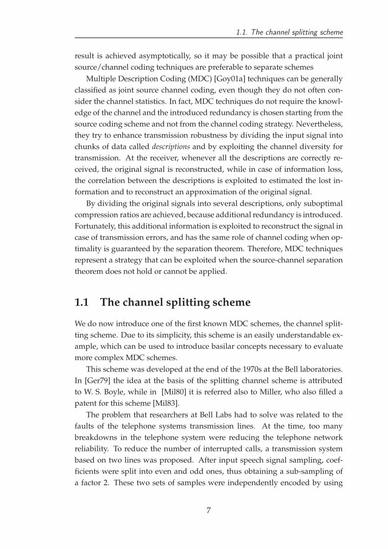
1.2.1 The MD RD region for the channel splitting scheme
From Equations (1.31), (1.32) and (1.33), we can write the following equation
for the channel splitting scheme:
Di ≥ σ22−2Ri , f ori = 1, 2 (1.59)
D0 ≥ σ22−2(R1+R2) · γD(R1, R2, D1, D2) (1.60)
where
γd =
1 i f D1 + D2 > σ2 + D01
1−(√
(1−D1)(1−D2)−√
D1D2−2−2(R1+R2))2 otherwise. (1.61)
00.5
11.5 0
0.51
1.5
0
0.1
0.2
0.3
0.4
0.5
0.6
0.7
0.8
0.9
1
R2
MD RD region Ozarow‘s bound for D0
R1
Dis
tort
ion
Figure 1.7: Bound for the multiple description rate-distortion region for the
channel splitting scheme in case of no redundancy and 50% coding
efficiency.
In Figure (1.7), the MD RD region is plotted in two cases: in case of hypo-
thetical no introduced redundancy (lower surface) and in case of 50% redun-
dancy. By losing efficiency, the MD RD region rises and the necessary bitrate
to obtain the desired quality becomes bigger. In the corner relative to R1 = 1.5
and R = 0 is possible to notice how the surface in case of increased bitrate
bends and becomes flat in a small region.
19

1.2. The MD RD region
In the balanced case, i.e. when R1 = R2 and D1 = D2, Goyal [Goy01b]
proved that the side distortion for a source with unit variance can be written
as
D1 ≥ min
{
12
[
1 + D0 − (1 − D0)
√
1 − 2−2(R1+R2)
D
]
,
1 −√
1 − 2−2(R1+R2)
D
}
(1.62)
under the constraint D1 > σ22−2R1 . Written in terms of base rate r = R(D0)
and redundancy ρ = R1 + R2 − R(D0),
D1 ≥{
12
[
1 + 2−2r −(
1 − 2−2r)√
1 − 2−2ρ]
f or ρ ≤ r − 1 log2(1 + 2−2r)
1 −√
1 − 2−2ρ f or ρ > r − 1 log2(1 + 2−2r)(1.63)
0 0.2 0.4 0.6 0.8 1 1.2 1.4 1.6 1.8 20
0.1
0.2
0.3
0.4
0.5
0.6
0.7
0.8Side distortion lower bound
Excess Rate Sum
Dis
tort
ion
varia
nce
r = 0.5r = 1r = 1.5r = 2
Figure 1.8: Bound for the multiple description rate-distortion region for the
channel splitting scheme in case of no redundancy and 50% coding
efficiency.
The obtained bound corresponds to the one provided by Ozarow evalu-
ated for the side distortion while keeping fixed D0. This bound is plotted Fig-
ure (1.8), for several excess rate sums. It is interesting to notice that the bound
has infinite slope when the excess rate sums is close to zero, then by increasing
20
1.2. The MD RD region
the rate it flattens and after that starts again to decrease, thus showing a behav-
ior similar to that of the central distortion. The interpretation given by Goyal
for the slope variation by increasing the excess rate sum is that at very low
bitrates a small additional rate will have more impact if dedicated to reducing
the side information that if dedicated to reducing the central distortion. In fact,
as it can be seen in Figure (1.7), by increasing the excess rate sum the bound
becomes flat in the origin because the bound rises to the maximum distortion,
which is the variance of the input signal. Thus there is no gain from allocating
the successive bits for the central decoder. These bits can be more efficiently
used to reduce the side distortion until also the side distortion bound becomes
flat and reducing the central distortion is more effective again. On the other
hand, at high bitrates both central and side distortion bounds have the same
exponential behavior and therefore the same efficiency is obtained, leaving the
freedom of an arbitrary rate allocation.
1.2.2 The Redundancy Rate-Distortion Region
As we have seen in the previous section, even in the case of a Gaussian source
and two channels the MD RD region is hard to evaluate. Whenever random
variables have a different p.d.f. or more complicated operations such as mo-
tion compensation, are performed, giving a full characterization of this region
becomes quickly impossible.
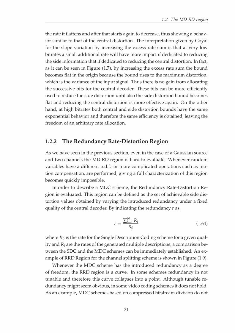
In order to describe a MDC scheme, the Redundancy Rate-Distortion Re-
gion is evaluated. This region can be defined as the set of achievable side dis-
tortion values obtained by varying the introduced redundancy under a fixed
quality of the central decoder. By indicating the redundancy r as
r =∑
Ni=1 Ri
R0(1.64)
where R0 is the rate for the Single Description Coding scheme for a given qual-
ity and Ri are the rates of the generated multiple descriptions, a comparison be-
tween the SDC and the MDC schemes can be immediately established. An ex-
ample of RRD Region for the channel splitting scheme is shown in Figure (1.9).
Whenever the MDC scheme has the introduced redundancy as a degree
of freedom, the RRD region is a curve. In some schemes redundancy in not
tunable and therefore this curve collapses into a point. Although tunable re-
dundancy might seem obvious, in some video coding schemes it does not hold.
As an example, MDC schemes based on compressed bitstream division do not
21
1.3. Applications to image and video coding
0 0.1 0.2 0.3 0.4 0.5 0.6 0.7 0.8 0.9 10
10
20
30
40
50
60Redundancy Rate−Distortion Region for the channel splitting scheme
Redundancy
SN
R (
dB)
Figure 1.9: Redundancy Rate Distortion region for the channel splitting
scheme.
have this possibility because it would be available only by re-encoding the se-
quence, but in this case transcoding is not allowed.
1.3 Applications to image and video coding
1.3.1 MD coding with Correlating Transforms
Transform-based source coding has been applied to many signal processing
problems to obtain coding gain and to enhance the compression quality. Sim-
ilarly, transforms can be adopted to generate two correlated signals from in-
dependent random variables. Correlation reduces coding efficiency, but at the
same time allows to estimate lost information from the received one.
A pairwise MD Correlating Transform is defined as
[
C
D
]
= T
[
A
B
]
. (1.65)
and its basic application for MDC is shown in Figure (1.10). Obviously, op-
timal reconstruction can be obtained only if the transformation T maps integer
into integer. A way to implement this transform is given by the lifting scheme
[CDSY98], which implements such lossless transform by expressing the lin-
22

1.3. Applications to image and video coding
Q
Q
Forward
PCT
Channel
Channel
Inverse
PCT
Q −1
Q −1
Estimator
for A, B
from D
Q −1
Q −1
Estimator
for A, B
from C
A~
~B
C
D^
A^
A^
A^
B^
B^
B^
D_C_
A
B
2 variable MD encoder
2 variable MD decoder
Figure 1.10: Basic scheme of coding and decoding process for a single pair.
ear application T with the LU decomposition. If the quantization step size is
denoted by Q, the transform and the quantized quantities can be expressed as
T =
[
a b
c d
]
(1.66)
A =
⌊
A
Q
⌋
(1.67)
B =
⌊
B
Q
⌋
(1.68)
W = B +
⌊
1 + c
dA
⌋
(1.69)
C = W −⌊
1 − b
dD
⌋
(1.70)
D = ⌊dW⌋ − A (1.71)
At the receiver, the original values can be reconstructed by inverting the
correlating transform
W = C +
⌊
1 − b
dD
⌋
(1.72)
A = ⌊dW⌋ − D (1.73)
B = W −⌊
1 + c
dA
⌋
. (1.74)
23

1.3. Applications to image and video coding
In case only one channel is correctly received, reconstruction requires an
estimate of the lost coefficient and inversion of the transform. The optimal
linear estimator is given by
γCD =σd
σCφ (1.75)
where φ is the correlation angle between C and D. Thus, the approximated
reconstructed signal is
[
A
B
]
= T−1
[
1σdσC
φ
]
CQ. (1.76)
In [OWVR97] it is suggested to use transforms of the form
T =
[
1 b
− 12b
12
]
(1.77)
while in [GK98] Goyal and Kovacevic extended the family of optimal trans-
forms to
T =
[
a 12a
−a 12a
]
. (1.78)
Finally, Wang et al [WOVR01] generalized the correlating transform in a
framework to realize MDC. They were able to evaluate the rate distortion anal-
ysis for a generic pairwise transform including distortion due to quantization
error, they were also able to prove that the family of transforms obtained by
Goyal is optimal even in the case of quantization. They summarize their result
as the optimal transform is formed by two equal length basis vectors that are rotated
away from the original basis by the same angle in opposite directions. This result im-
plies that orthogonal transform is not optimal and it has the same performance
as the optimal one only when the introduced redundancy is either null or at its
maximum possible value.
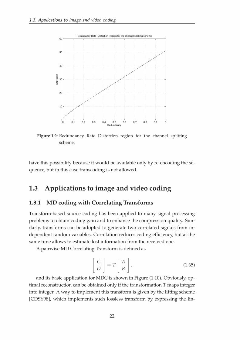
In case more than two random variables have to be encoded and transmit-
ted over different channels at the same time, the cascade structure proposed
in [GK98] can be used. As shown in Figure (1.11) variables are pairwisely
transformed and successively another transform is applied to correlate a vari-
able from each previously correlated pair.
Several application of this techniques have been proposed in literature.
Most of them aim to protect the transformed values of the DCT coefficients.
As an example, in [GKAV98] it is applied to JPEG image coding by applying
the following steps
24
1.3. Applications to image and video coding
T^
β
T^
α T^
γ
T^
γ
x 1
x 3
x 2
x 4
y 1
y 3
y 2
y 4
Figure 1.11: Cascade structure allows simple and efficient coding for more
than two channels.
• A 8x8 block DCT of the image is computed;
• The DCT coefficient are uniformly quantized;
• Vectors of length 4 are formed from DCT coefficients separated in fre-
quency and space;
• Correlating transforms are applied to each 4-tuple;
• Entropy coding akin to that of JPEG is applied.
1.3.2 MD coding with Frames
Another example of MDC is given by Frames, which are obtained with linear
transforms.
The theory of filter banks [Vai93a] and [VK95] provides a framework for
a class of signals decompositions in l2(Z), based on signal analysis through a
sliding window by using a set of elementary waveforms. In general, an expan-
sion can be written as
x[n] =K−1
∑i=0
+∞
∑j=−∞
ci,jφi,j[n] (1.79)
where the vectors φi,j[n] are the translated versions of K elementary wave-
forms
φi,j[n] = φi[n − jN] (1.80)
with N ≤ K. If the family Φ
Φ ={
φi,j : φi,j[n] = φi[n − jN], i = 0, 1, · · · , k − 1, j ∈ Z}
⊂ RN (1.81)
25

1.3. Applications to image and video coding
is a frame, then any signal in l2(Z) can be represented in a numerically
stable way.
The family of vectors in Equation (1.81) is a frame if for any x ∈ l2(Z) exist
some constants A > 0 and B < ∞ such that
A ||x||2 ≤K−1
∑i=0
+∞
∑j=−∞
∣
∣< x, φi,j >
∣
∣
2 ≤ B ||x||2 . (1.82)
If the family Φ is a frame, then there exists another frame
Ψ ={
ψi,j : ψi,j[n] = ψi[n − jN], i = 0, 1, · · · , k − 1, j ∈ Z}
(1.83)
such that the coefficients of the expansion (1.79) can be calculated as inner
product with its vectors, that is
x[n] =K−1
∑i=0
+∞
∑j=−∞
< x, ψi,j > φi,j[n]. (1.84)
In case A = B, then the frame is said to be tight and Φ is equal to Ψ and the
expansion formula (1.79) can be written, similarly to orthogonal expansions,
as
x[n] =1
A
K−1
∑i=0
+∞
∑j=−∞
< x, φi,j > φi,j[n] (1.85)
where the term 1A is necessary because the transform is orthogonal but not
orthonormal.
If K > N, the transform is not a bijection, thus the expansion is a redundant
representation. Since the transform is no longer injective, its kernel does not
consists only of the null element, and therefore only N coefficients are required
to be correctly received to reconstruct the signal.
Oversampling of a periodic, band-limited signal can be seen as a frame
operator applied to the signal, where the frame operator is associated with a
tight frame. Let x = [x1, x2, · · · , xn]T ∈ RN, with N odd. By exploiting the
inverse Fourier transform, a continuous time signal can be written as
xc(t) = x1 +
N−12
∑k=1
[
x2k
√2 cos
2πkt
T+ x2k+1
√2 sin
2πkt
T
]
(1.86)
If we define a sampled version of xc(t) as xd[m] = xct(
mTM
)
, assuming M ≥N and by indicating
y = [xd[0]xd[1] · · · xd[M − 1]]T (1.87)
26
1.3. Applications to image and video coding
than y = Fx, with
F = [φ1φ2 · · · φm]T (1.88)
and
φk =
[
1,√
2 cos2πk
M,√
2 sin2πk
M, · · · ,
√2 cos
2π N−12 k
M,√
2 sin2π N−1
2 k
M
]
.
(1.89)
It is easy to verify that F is a tight operator, whose columns have norm√
N.
By dividing F by√
N the frame is normalized and frame bound corresponds
to the introduced redundancy.
Frame expansion from RN to R
K can be considered as a (K, N) block code,
where in case up to K − N coefficients are lost perfect reconstruction is possi-
ble. Whenever less then N coefficients are correctly received, estimating x can
be posed as a simple least-squares problem. Thus, the estimate of the original
signal can be obtained by multiplying the received vector with the pseudoin-
verse matrix of F
x = F+y = F+Fx (1.90)
In [GVT98], a better estimate is proposed, which considers distortion caused
by uniform quantization which brings to a Linear Programming problem.
An application of frame expansion to JPEG images is given in [GKAV98],
where a 10 × 8 frame operator F corresponding to a length 10 Discrete Fourier
Transform of a length 8 sequence is used. The coding approach proceeds as
follows:
• An 8x8 block DCT of the image is computed;
• Vectors of length 8 are formed from DCT coefficients of same frequency,
separated in space;
• Each length 8 vector is expanded by left multiplication with F;
• Each length 10 vector is uniformly quantized
1.3.3 MD coding with Motion Compensation
In case of video coding, not only spatial redundancy but also temporal redun-
dancy can be exploited. This additional degree of freedom allows many more
27
1.3. Applications to image and video coding
schemes, but at the same time makes harder to evaluate theoretically the per-
formance of such MDC schemes.
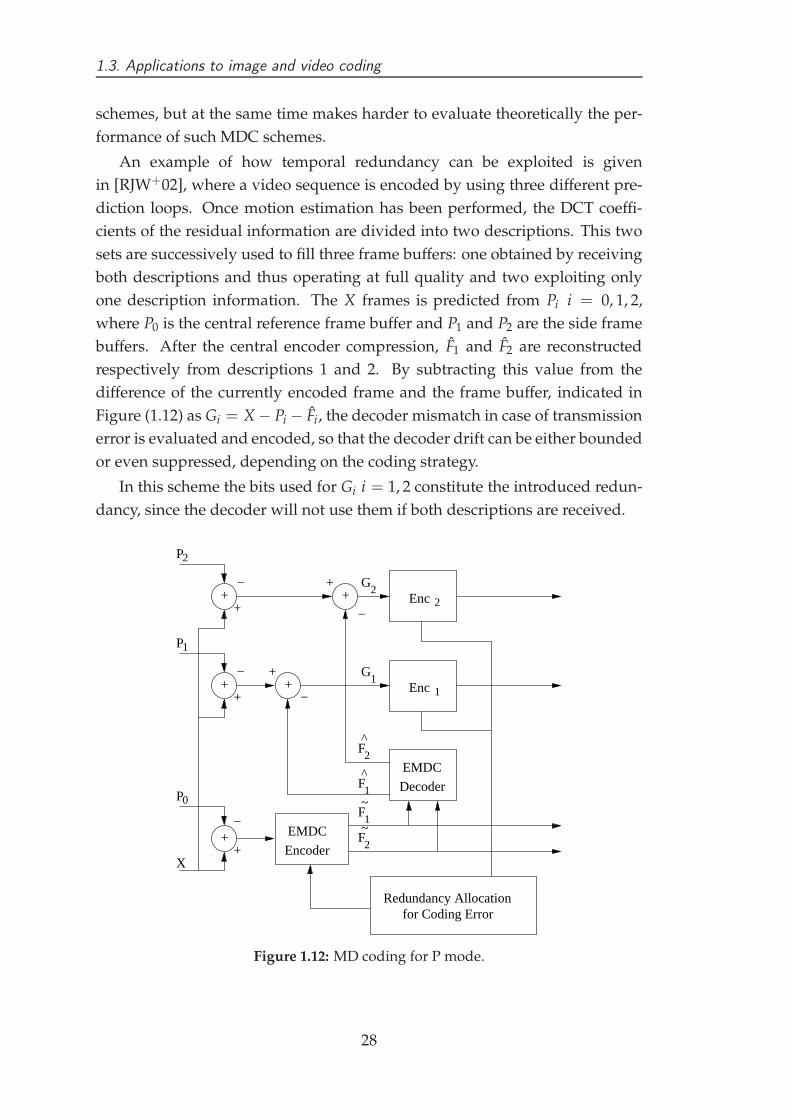
An example of how temporal redundancy can be exploited is given
in [RJW+02], where a video sequence is encoded by using three different pre-
diction loops. Once motion estimation has been performed, the DCT coeffi-
cients of the residual information are divided into two descriptions. This two
sets are successively used to fill three frame buffers: one obtained by receiving
both descriptions and thus operating at full quality and two exploiting only
one description information. The X frames is predicted from Pi i = 0, 1, 2,
where P0 is the central reference frame buffer and P1 and P2 are the side frame
buffers. After the central encoder compression, F1 and F2 are reconstructed
respectively from descriptions 1 and 2. By subtracting this value from the
difference of the currently encoded frame and the frame buffer, indicated in
Figure (1.12) as Gi = X − Pi − Fi, the decoder mismatch in case of transmission
error is evaluated and encoded, so that the decoder drift can be either bounded
or even suppressed, depending on the coding strategy.
In this scheme the bits used for Gi i = 1, 2 constitute the introduced redun-
dancy, since the decoder will not use them if both descriptions are received.
+
+ +
P1
P2
+ Enc 2
Enc 1
Redundancy Allocationfor Coding Error
EMDC
Decoder
EMDC
Encoder+
P0F
1
~
F2
~
F2
^
F1
^
G1
G2
X+
+
+
+
+
−
−
−
−
−
Figure 1.12: MD coding for P mode.
28

1.3. Applications to image and video coding
Multiple descriptions are generated in the EMDC by applying a Pairwise
Correlating Transform (PCT) to couples of DCT coefficients, in order to reintro-
duce some redundancy after it has been removed by the DCT. After the PCT,
coefficients are split in even and odd and they are encoded with the motion
vector field, which is copied in both descriptions, together with the mismatch
control signal Gi.
There are several possibilities to generate the mismatch control signal, which
bring to different results:
• Full mismatch control: from each description, lost information is esti-
mated by exploiting the PCT. The drift signal Gi is formed by subtracting
Fi, the image reconstructed from only one description, from the original
image X and also subtracting the relative prediction Pi. Once Gi has been
evaluated, it is encoded as Intra, by applying the DCT and by quantiz-
ing with a quantization step size bigger than the step size of the central
encoder, thus reducing the introduced redundancy. The main drawback
of this approach consists of expanding the original information. In fact,
in case of channel fault, only 32 coefficients of the 8x8 block are not re-
ceived, but the Intra coding in the side encoders works on the full set of
64 values.
• Partial mismatch control: the problem of information expansion is ad-
dressed in the side encoders. Rather than completely encoding Gi, only
the more important part of the signal is extracted, so that only 32 coeffi-
cients are transmitted. The central encoder sends the central prediction
error, X − P0, while the side loop sends the difference between a linear
estimate of the transmitted image and the side-loop prediction error.
• No mismatch control: in this case no prediction loop is used in the side
decoders. Redundancy is no more used to encode the drift signal Gi, but
is it used to enhance the quality of each Single Description decoder.
29

1.3. Applications to image and video coding
30
Chapter 2
H.264/AVC-based MDC schemes
2.1 Introduction to H.264/AVC
The H.264/AVC [WSBL03] is a standard for video compression. It is also
known as MPEG-4 Part 10, or MPEG-4 AVC (for Advanced Video Coding).
It was written by the ITU-T Video Coding Experts Group (VCEG) together
with the ISO/IEC Moving Picture Experts Group (MPEG) as the product of a
partnership effort known as the Joint Video Team (JVT).
The final drafting work on the first version of the standard was completed
in May 2003 and in the successive years it has been extended. In the mean-
while, it has been adopted in always more products.
Post−Processing& Error Recovery
Pre−Processing Encoding
Decoding
Source
Destination
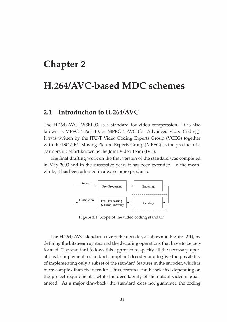
Figure 2.1: Scope of the video coding standard.
The H.264/AVC standard covers the decoder, as shown in Figure (2.1), by
defining the bitstream syntax and the decoding operations that have to be per-
formed. The standard follows this approach to specify all the necessary oper-
ations to implement a standard-compliant decoder and to give the possibility
of implementing only a subset of the standard features in the encoder, which is
more complex than the decoder. Thus, features can be selected depending on
the project requirements, while the decodability of the output video is guar-
anteed. As a major drawback, the standard does not guarantee the coding
31

2.1. Introduction to H.264/AVC
efficiency, whose responsibility is due to the encoder implementation and its
coding strategy.
Dn’
nDT Q
T −1 Q−1
ReorderEntropy
encodeFn
n
nF
F ’
’ Fn’u
(current)
(reference)
(reconstructed)Filter
ME
ChooseIntra
prediction
Intraprediction
MC
Intra
Inter
P
+
+
−
+ X NAL
Figure 2.2: Block scheme of the H.264/AVC encoder.
The H.264/AVC encoder is organized in a closed-loop structure. Each frame
can be encoded either as Intra or Inter. In the first case, it can be independently
decoded, while in case temporal prediction is used, valid reference frames are
necessary for motion compensation. After spatial or temporal prediction, the
difference signal is transformed and quantized and the obtained values are
compressed with entropy coding.
The quantized values are used, together with the information relative to
the prediction, to reconstruct the same frame that is decoded at the receiver
along the so called reconstruction path, which is the path at the bottom of the
block scheme of Figure (2.2). By using the reconstructed frame as reference
for the successive ones, the encoder is able to compensate the drift that quan-
tization generates at the decoder and to assure better reconstruction quality.
Since the decoder needs to perform both encoding and decoding, it can be eas-
ily understood why in the H.264/AVC standard such a freedom of choosing
functionalities is given.
2.1.1 Intra prediction
The H.264/AVC standard provides three main Intra prediction modes for the
luminance component, which are supported in all slice types.
The Intra 4x4 mode is based on encoding all 4x4 pixel blocks of each mac-
roblock independently. Each 4x4 block is spatially predicted from the already
32

2.1. Introduction to H.264/AVC
encoded adjacent blocks, by using one of the nine prediction modes, shown in
Figure (2.3). With the exception of the DC mode which can be adopted in case
of uniform regions, these prediction modes are suited to predict textures with
well identified structures.
Spatial prediction in the image domain is a feature that in not present in
previous coding standard. In fact, in H.263 and MPEG-4 intra prediction is al-
ways performed in the frequency domain. This new strategy is able to provide
a better estimate of non smooth regions in the frame.
In case the macroblock is uniform, the Intra 16x16 mode can be adopted.
For this type of prediction, only four prediction modes are available: 0 - ver-
tical, 1 - horizontal, 2 - DC, 3 - plane. This four modes are the same available
for the two chrominance components, with the difference of the mode num-
ber. In this case, mode numbers are 0 - DC, 1 horizontal, 2 - vertical and 3 -
plane. The prediction mode is shared between the two chrominance compo-
nents and if any chrominance block is encoded as Intra 16x16, then both blocks
are encoded in this way.
As an alternative to Intra 4x4 and 16x16 is the Intra I_PCM mode, which
bypasses prediction and transform coding and directly send the values of the
encoded pixels. This mode has the following purposes:
• it offers the possibility of exactly transmitting the values of the frame
pixels;
• it provides a strategy to encode parts of the image where excess of details
would cause an anomalous bitstream size increment without quality en-
hancement;
• it provides an upper bound to the bandwidth necessary to encode the
block as Intra.
2.1.2 Motion estimation
In comparison to prior video coding standards, H.264/AVC has some features
that significantly increase the achievable compression ratio.
In previous coding standards, the size of blocks used for motion estimation
is 16x16 or 8x8 pixels. In H.264/AVC, each macroblock can be partitioned in
one block of 16x16 pixels, two 16x8 pixels blocks, two 8x16 pixels blocks or four
blocks of 8x8 pixels each. In this case each 8x8 partition can be further split in
two 8x4, two 4x8 or four 4x4 partitions. Available partitions and sub-partitions
are shown in Figure (2.4)
33

2.1. Introduction to H.264/AVC
Mode 0 − Vertical Mode 1 − Horizontal Mode 2 − DC
Mode 3 − Diagonal down left Mode 4 − Diagonal down right
Mode 8 − Horizontal up
Mode 5 − Vertical right
Mode 7 − Vertical left
Mode 6 − Horizontal down
+
+
+
+
+ + +
Figure 2.3: The nine Intra 4x4 prediction modes.
34

2.1. Introduction to H.264/AVC
001 10
0 1
32TypesM
0Types8x8 0
1 100 1
32
16x16 16x8 8x16 8x8
8x8 4x44x88x4
Figure 2.4: Segmentations of the macroblock for motion compensation. Top:
partitions of macroblocks. Bottom: possible sub-partitions of 8x8
pixels blocks.
Motion compensation is performed on the luminance component with one
quarter of pixel accuracy [Wed03]. To generate sub-pixel values, interpolation
is applied twice to the reference frame. In the first step, half pixels values
are generated by applying a separable FIR filter, which can be realized as the
application of a one-dimensional 6-tap FIR filter horizontally and vertically.
The filter coefficients are
h = {1,−5, 20, 20,−5, 1} , (2.1)
and the final interpolated value is obtained by adding sixteen and dividing
by thirty-two, so that its value is clipped to the range 0-255. The quarter pixel
values are derived by averaging with upward rounding of the two nearest
samples at integer and half integer positions.
Since the chrominance components are low-pass signals, the filtering oper-
ation always consists of bilinear interpolations. Furthermore, since the chromi-
nance sampling grid has a reduced resolution if compared to the luminance
grid, the displacements used for chrominance compensation have one eight
pixel accuracy.
To further increase compression, motion vectors can refer to regions out-
side the picture boundaries. In this case, non existing pixels are extrapolated
by repeating the values of the pixels on the frames edges before interpolation.
Moreover, several frames can be used as reference while performing motion
estimation, as shown in Figure (2.5). While exploiting this feature, both the
encoder and the decoder need to maintain in memory the same multi-picture
buffer. Unless the multi-picture buffer consists of only one picture, the ref-
erence index parameter has to be encoded for each 16x16, 18x8, 8x16 or 8x8
luminance block. In case a 8x8 block is sub-partitioned, the same reference
35

2.1. Introduction to H.264/AVC
index is shared between the sub-partitions.
2 Prior Decoded Framesas References
Current f\Frames
∆=2∆=1
Figure 2.5: Example of multi-picture motion compensation. To correctly iden-
tify the reference, the parameter ∆ for each 16x16, 16x8, 8x16 and
8x8 is transmitted.
Along to the explained prediction modes, H.264/AVC offers a special mode
called P_SKIP. This prediction mode is equivalent to the 16x16 mode with a
null motion vector prediction referring to the first image of the multi-picture
buffer. This prediction mode leads to extremely high compression ratios, be-
cause large areas can be transmitted with only a few bits. Since the motion
vector field is differentially encoded by using the median of adjacent motion
vectors, the P_SKIP mode can be used not only to encode static portions of the
frame, but also zones characterized by slow uniform panning.
The H.264/AVC standard has also the possibility of encoding inter-frames
using two reference frames. In case of B prediction, all the features for P frames
are available, and the main difference is that B macroblocks can use a weighted
average of two distinct motion-predicted frames as references. To make use of
multi-picture references in B frames, the encoder and decoder utilize two lists
of reference frames, called list 0 and list 1. This two lists are used for four
different type of prediction: list 0, list 1, bi-predictive and direct. In the first
two cases only one frame is used as reference, while in the bi-predictive case
the weighted average of two frames is used as reference. In the direct case, the
prediction is automatically inferred from previously transmitted information.
For B frames the B_SKIP mode plays the same role as P_SKIP in P frames:
the motion vector is the median of the adjacent partitions and no residual in-
formation is transmitted.
36

2.1. Introduction to H.264/AVC
2.1.3 Integer transform
As in many coding schemes, the residual signal obtained after prediction is
compressed with transform coding. The main differences between the H.264/AVC
transform and the transforms adopted in earlier standard consist of its size,
which is 4x4 pixels, and of the adoption of an integer transform with proper-
ties similar to a DCT.
The transform matrix, given as
T =
1 1 1 1
2 1 −1 −2
1 −1 −1 1
1 −2 2 −1
, (2.2)
consists only of integer values of one ad two. This choice has several ad-
vantages:
• it does not require a floating point ALU to be executed and it needs only
sixteen bits of precision instead of other floating point solutions which
need up to thirty-two bits;
• it can be easily implemented as sums, differences and shifts, thus it can
be efficiently parallelized;
• it does not suffer from decoder drift, as it happens with fixed point ap-
proximation of DCT coefficients across different architectures and CPUs.
The quantization parameter QP determines the quantization step size of
coefficients in H.264/AVC. The value of this parameter spans from 1 to 52
and each increment of 1 corresponds approximately to a 12% increment of the
quantization step size. This reflects approximately in a 12% growth of the en-
coded bitstream.
In order to keep computational efficiency high, quantization and some scal-
ing products due to the 4x4 transform are performed together, without having
to manipulate the coefficients twice.
Successively, with the adoption of the Fidelity Range Extensions [MWG05],
the integer transform has been extended to the size of 8x8 pixels. In my tests
the size increment did not lead to higher compression ratios, as it could be ex-
pected, but it reduced the time needed to encoded each frame. The unchanged
coding efficiency is due to the very precise prediction that is at the basis of
H.264/AVC performance. The reduced complexity and increased speed make
37

2.1. Introduction to H.264/AVC
this solution suitable for encoding sequences with very large frames, where
big regions are uniform.
2.1.4 Entropy coding
Once coefficients have been transformed and quantized, they are entropy en-
coded. H.264/AVC offer two coding engines for this purpose: the Context-
Adaptive Variable Length Coding (CAVLC) and the Context-Adaptive Binary
Arithmetic Coding (CABAC).
In CAVLC, several tables are defined to match the possible coefficients
statistics that the encoder might encounter. These tables are used to encode
the zig-zag scan of the quantized values of 8x8 blocks, starting from those cor-
responding to high frequencies and moving towards those at low frequencies.
The reason of this strategy is that high-frequency coefficients are often null
and their absolute value increases while moving towards low-frequency co-
efficients. To fully exploit this statistics, CAVLC encodes for each block the
number of non-null coefficients and successively encodes the values by using
run-length encoding. Moreover, since the initial non null coefficients in the
zig-zag scan have a high probability of having absolute size 1, together with
the number of non-null coefficients the number of trailing ones is saved. This
information efficiently indicates the presence of up to three coefficients of ab-
solute value 1 at the beginning of the run-length encoding.
The length of runs is encoded by saving the information of the total number
of null coefficients in the zig-zag scan. After that, for each non-zero value the
number of zeros before that coefficient is signaled, thus the position of zeros
in the zig-zag scan can be reconstructed. In case all the null coefficients have
already been encoded in the scan, the number of zeros is omitted to increase
coding efficiency, since all the successive runs will have length 0.
H.264/AVC offers the possibility of using arithmetic encoding with
CABAC [DMW03], which is based on assigning a not-integer number of bits
to each encoded value to further reduce the bitstream size. Two are the key
properties of CABAC: coefficient binarization and context adaptivity. Each en-
coded value is transformed into a string of zeros and ones, where the symbols
probabilities are not equal. Thus, the arithmetic encoder is able to fully exploit
this statistics to efficiently compress the string of bits. Further more, CABAC
contexts are dynamically modeled: previously encoded syntax elements are
used to adapt to non-stationary symbol statistics.
By adopting CABAC, the output bitstream size has a reduction between 5%
and 15%. On the other hand, complexity and computational requirements are
38

2.1. Introduction to H.264/AVC
increased, even though the arithmetic coding engine and probability estima-
tion algorithms are specified as multiplication-free operation, in order not to
require excessive additional computational power.
2.1.5 In-loop deblocking filter
Block-based compression algorithms often leads to distortion that manifests
itself as the production of visible block structures. The main reason of these
blocks is the quantization of the transformed coefficients. In fact, each element
of the transform basis can be seen as a set small blocks and quantization can
be compared to adding a linear combination of scaled elements of the basis
functions to the original image.
To reduce this distortion, H.264/AVC defines an adaptive in-loop deblock-
ing filter [LJL+03], whose effect is modulated by the values of several syntax
elements. The filter works mono-dimensionally on 4x4 block edges and takes
into account up to three pixel in each 4x4 block, as shown in Figure (2.6).
p0
p2
p1
q0
q1
q2
Figure 2.6: Deblocking filter mechanism.
The filter modifies p0 and q0 only if all the following conditions are matched:
• |p0 − q0| < α(QP)
• |p1 − p0| < β(QP)
• |q1 − q0| < β(QP) .
p1 and q1 are filtered if the corresponding following condition is satisfied:
39

2.2. Test conditions
• |p2 − p0| < β(QP)
• |q2 − q0| < β(QP) .
The heuristic of this adaptive filter is based on the assumption that a large
absolute difference between adjacent samples indicates the presence of block-
ing artifacts, while small gaps are due to the frame texture and it does not have
to smooth them.
As expected, this filter does not reduce sharpness while reducing distor-
tion. This reflects in better subjective quality and in bitstream size reduction
between 5% and 10%.
2.2 Test conditions
There are several factors that can influence a MDC scheme performance, espe-
cially in case of image and video coding because error concealment techniques
can be adopted. In case of video sequences, also the choice of the Group Of
Pictures (GOP), its length and the number of P and B frames can significantly
change the decoded quality.
In [PA97] and [Per99] three test cases, shown in Table (2.1), are defined
to test transmission in error-prone environments. As suggest in other arti-
cles, during the development of the MDC schemes based on H.264/AVC we
adopted test case number 2 for our test conditions. This case requires the cor-
ruption of the bitstream to introduce three 16 to 24 ms long bursts of errors
separated by 2 s and 1.5 s far from the beginning of the sequences in order to
allow the decoder to correctly synchronize with the stream.
Since at the time we did not have a robust decoder able to deal with a
corrupted bitstream and since the worst-case burst is 2 ms long, we decided to
approximate the test conditions with the loss of a frame description. In fact,
24 ms corresponds to 41 frames per second. In case of a sequence at 20 frames
per second, in case of MDC with two descriptions, 40 packets per second are
necessary and therefore the single packet loss is compatible with the test case.
Moreover, since the error bursts are separated by two or more seconds, we
decided to consider only one error per GOP.
All the H.264/AVC MDC schemes were tested adopting these conditions.
40

2.3. Sub-Sampling Multiple Description Coding
Test case Residual error conditions Description Error interval
[begin, end] (s)
1 10−3 High Random BER [1.5, end]
2 3 burst of errors Multiple burst errors [1.5, 8]
50% BER within burst
Random Burst Length:
16 to 24 ms
Random Bursts Separation:
> 2s
3 Combination of test cases High random BER [1.5, end]
1 and 2 and multiple burst errors
Table 2.1: Error-prone video channel conditions.
2.3 Sub-Sampling Multiple Description Coding
Due to the high spatial correlation within a frame, each pixel may be estimated
according to its neighbors. Consequently, a MD scheme can be defined by
grouping adjacent pixels into separate descriptions. This operation is repre-
sented in Figure (2.7).
LPF
LPF
LPF
LPF
4x
4x
4x
4x Channel 4
Channel 3
Channel 2
Channel 1
x(2i+1,2j+1)
x(2i,2j+1)
x(2i+1,2j)
x(2i,2j)
H.264/AVC
H.264/AVC
H.264/AVC
H.264/AVC
Figure 2.7: Multiple Description transmission using the sub-sampling ap-
proach of the SMDC coder.
Each input frame is sampled along its rows and columns with a sampling
factor of 2. Let x(i, j) be the luma sample of the current frame at position (i, j),
then the four sub-sequences are respectively formed with pixels
41

2.3. Sub-Sampling Multiple Description Coding
0 500 1000 1500 2000 250026
28
30
32
34
36
38
40
40
40
36
36
32
32
28
28
24
24
Rate−Distortion
Rate
PS
NR
Y (
dB)
Foreman SDForeman MD
Figure 2.8: SMDC Rate-Distortion functions for the “foreman” and “mobile”
CIF sequences.
x(2i , 2j) first sub-sequence
x(2i + 1 , 2j) second sub-sequence
x(2i , 2j + 1) third sub-sequence
x(2i + 1 , 2j + 1) fourth sub-sequence
In this way, for each input sequence the scheme generates four
sub-sequences with halved resolution on both spatial directions, and a size
of one fourth of the original sequence size. Figure (2.8) gives an example of the
Rate-Distortion functions for sequences “foreman” and “mobile”. The curves
are parameterized as a function of the QP parameter. From the results shown,
it is apparent that the scheme may introduce a considerable redundancy in the
case of “hard-to-code” sequences.
Each sub-sequence is sent to a separate H.264/AVC coder, and the output
bitstreams are sent to four independent channels. In the case that only one of
the descriptions arrives at the receiver, the end-user is able to reconstruct the
coded sequence at lower resolution without any artifact or channel distortion.
When more sequences arrive, the decoder can estimate the lost information ex-
ploiting the correlation among neighboring pixels. In this approach, assuming
42

2.3. Sub-Sampling Multiple Description Coding
0 5 10 15 20 25 30 35 40 45 5026
26.5
27
27.5
28
28.5
29
29.5
30
30.5Foreman QP 32
frame NO
PS
NR
Y (
dB)
MD (no error)MD (1 error)MD (2 errors)
Figure 2.9: PSNR as a function of the frame number when none, one or two
descriptions are lost in the “foreman” CIF sequence.
that pixel x(2i , 2j) belongs to the lost description, the missing pixel is replaced
with the mean of the available pixels.
Figure (2.9) shows an example of the recovering capabilities of the SMDC
scheme when one or two descriptions are lost. As a comparison, the results of
the no losses case is also given. Note that the PSNR loss is about 1 dB when
three descriptions arrive and about 2 dB when two descriptions arrive.
However, it is worth noticing that also when no channel errors occur, the
full resolution sequence is reconstructed with some small artifacts. This anoma-
lous behavior is mainly due to small differences of the compression gain be-
tween the four encoders which manifests itself as a spatial non-homogeneous
quality, visible at low bitrates. Correlating filters were adopted in order to
address this problem and to obtain a more efficient reconstruction of the full
resolution sequence. However, the performance of such filters was seriously
affected by the data intrinsic correlation, and negligible improvements were
obtained.
It is worth to note that the SMDC scheme is a particular case of the frame-
based MDC scheme where additional descriptions are added with a correlat-
ing transform [RMR+04, BRTV04]. However, there is a relevant drawback to
this kind of solution, i.e. the high correlation between the coded streams usu-
43
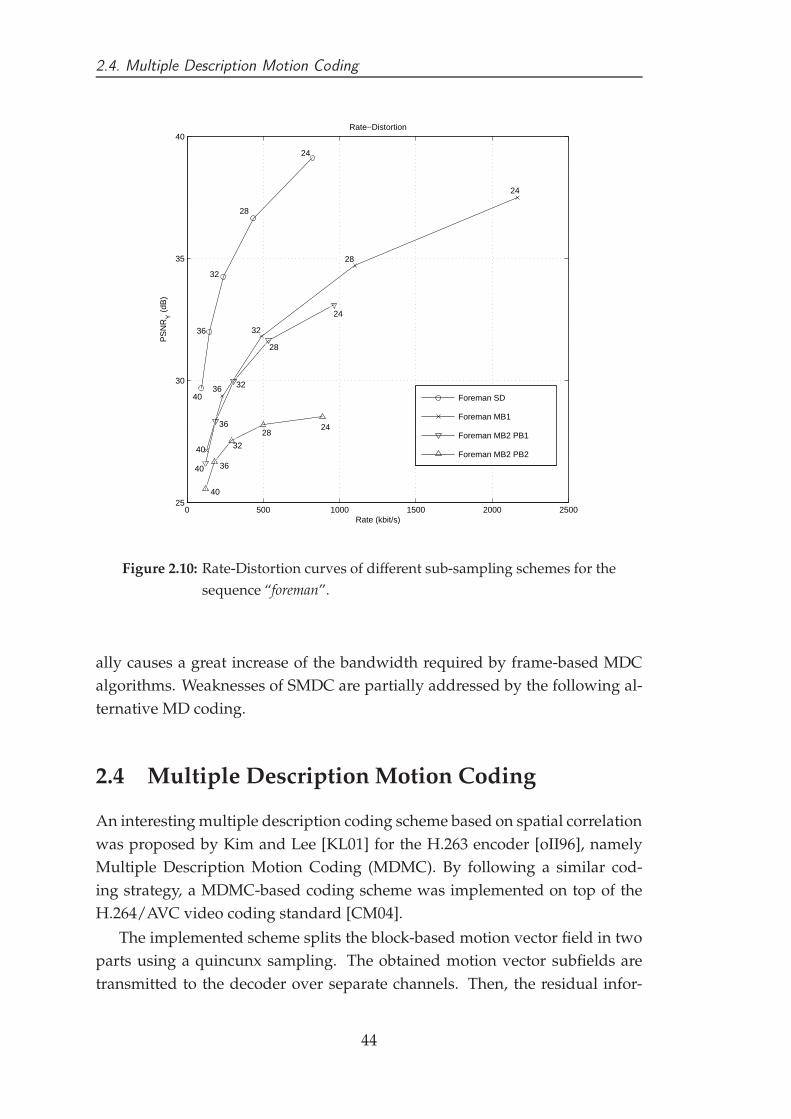
2.4. Multiple Description Motion Coding
0 500 1000 1500 2000 250025
30
35
40
Rate (kbit/s)
PS
NR
Y (
dB)
Rate−Distortion
Foreman SD
Foreman MB1
Foreman MB2 PB1
Foreman MB2 PB2
40
40
40
40
36
36
36
36
32
32
32
32
28
28
28
28
24
24
24
24
Figure 2.10: Rate-Distortion curves of different sub-sampling schemes for the
sequence “foreman”.
ally causes a great increase of the bandwidth required by frame-based MDC
algorithms. Weaknesses of SMDC are partially addressed by the following al-
ternative MD coding.
2.4 Multiple Description Motion Coding
An interesting multiple description coding scheme based on spatial correlation
was proposed by Kim and Lee [KL01] for the H.263 encoder [oII96], namely
Multiple Description Motion Coding (MDMC). By following a similar cod-
ing strategy, a MDMC-based coding scheme was implemented on top of the
H.264/AVC video coding standard [CM04].
The implemented scheme splits the block-based motion vector field in two
parts using a quincunx sampling. The obtained motion vector subfields are
transmitted to the decoder over separate channels. Then, the residual infor-
44

2.4. Multiple Description Motion Coding
mation of each macroblock is multiplexed on the two streams, by saving it in
one description for even macroblocks and in the other stream for the odd ones.
Moreover, some further constraints have been imposed on the design of the
scheme. First, each generated description has to be entirely decodable so that
in case a whole description is lost, the receiver is able to decode the other one
and to reproduce the sequence at a lower visual quality. Second, the compu-
tational overhead introduced by the MDC has to be kept as low as possible
in order to reduce the computational requirements of the coder and to permit
real time execution.
Both these goals have been achieved modifying the scheme of the stan-
dard H.264/AVC coder, as shown in Figure (2.11). In the general scheme,
we included an additional block, called Multiple Description Layer (MDL), be-
tween the Network Abstraction Layer and the Transport Layer. The task of the
new layer is to divide the bitstream provided by the H.264/AVC coder and
to generate the two descriptions. Some information is repeated on both the
bitstreams, while some other information is only included in one of them. In
this way, the whole motion estimation is performed only once inside the Single
Description coder (SDC), and the new layer only needs to split the information
and to rewrite some syntax elements.
The descriptions are obtained copying the initial SPS and PPS headers on
both streams as well as all the SH headers, while the slice data are divided into
two parts. The motion vector information of each macroblock is partitioned
using an evolution of the quincunx sampling used by Kim and Lee in [KL01].
This extension is necessary because the H.264/AVC coding standard permits
further partitioning into blocks of different sizes, while the previous coding
standard H.263 supported only 8x8 pixels blocks. The motion vectors that do
not belong to the current description are substituted with null vectors since
they require the lowest number of bits per component to be coded, i.e. only
one. This substitution allows the system to get a syntactically correct bitstream
while the increment of the overall bit rate is reduced to a minimum. The DCT
residual information is alternatively included in one of the two descriptions,
as Figure (2.12) shows. Whenever the coefficients are not available in the cur-
rent description, they are considered null by setting the coded_block_pattern
parameter to zero. In this way, each coded bitstream preserves the H.264/AVC
syntax and can be correctly decoded. At the receiver side, whenever both the
descriptions are received the MDL merges them together recovering the orig-
inal bitstream with an operation that is the dual version of the partition per-
formed at the transmitter.
45

2.4. Multiple Description Motion Coding
Video Coding Layer
Data Partitioning
Control Data
Network Abstraction Layer
Transport Layer
Multiple Description Layer
Figure 2.11: Scheme of the proposed coder/decoder. The dotted box repre-
sents the new Multiple Description Layer added to the original
H.264/AVC scheme.
The splitting process presents some problems due to the context-based en-
tropy coding algorithms, CABAC and CAVLC, which were adopted in the
H.264/AVC standard. In the MDL we only support the semantics of the
CAVLC because in case of loss of one description, the CABAC-coded bitstream
is more vulnerable to errors. In order to provide evidence for the weakness of
the CABAC algorithm, we can consider how the motion vectors are coded.
The coding context is chosen according to the information of the blocks on the
left and above the current one. Whenever a description is not available, lost
motion vectors have to be estimated according to the neighboring ones. This
operation increases the probability of selecting a wrong context model and can
seriously compromise the correct decoding of the rest of the frame. On the
other hand, although the CAVLC algorithm can achieve only a slightly infe-
rior performance, it is more robust to errors.
In the splitting process, some problems arise while decoding the residual
information. The residual information of every macroblock in H.264/AVC is
partitioned into sixteen blocks of 4x4 pixels before the coding process. The
CAVLC algorithm uses the number of quantized coefficients different from
zero of the blocks on the left and above the current block. Since the coefficients
46

2.4. Multiple Description Motion Coding
Figure 2.12: Splitting example: quincunx sub-sampling is applied to the mo-
tion vector filed of the four macroblocks and residual information
is saved for even macroblocks in one description and for the odd
ones in the other description.
of adjacent macroblocks are included in different descriptions by the splitting
process, the merging routines of the MDL can not decode them correctly un-
less a transcoding is performed before sending the information over the two
channels. In every macroblock, the upper and left 4x4 pixel blocks need to
be transcoded, while the other nine blocks can be sent with not changes. The
transcoding operation rewrites the coeff_token, which is the syntax element
that contains the information about the number of quantized block coefficients
different from zero. The bit string used to code the coeff_token is selected
between several VLC tables, and it has to be changed for the upper and left
blocks. In fact, during the splitting process the coefficients of the blocks be-
longing to the adjacent macroblocks have been set to zero, and the MDL needs
to change the actual coding context. An example is shown in Figure (2.13). In
the same way, a dual transcoding operation is performed at the receiver side
during the merging process in order to update correctly the decoding context
and to recover the original bitstream.
In case of loss of one description, the lost motion vectors are estimated by
the mean of the adjacent ones, while the lost coefficients are not recovered.
The redundancy has been estimated measuring the percentage increment
between the overall bit rate of the two MD streams and the original one. In
our scheme, the allocated redundancy can not be controlled by reducing the
perceptual quality as other MDC schemes do, but it is an intrinsic property of
the coded sequences.
Figure (2.14) shows that the added redundancy for sequence “foreman” in-
creases with the quantization parameter QP, that it is to say that the percentage
of redundancy decreases for a video sequence coded at a higher visual quality.
47

2.4. Multiple Description Motion Coding
11
2 2 4
2 2
2 2 53
3 02 2
3
1
1
2
03 2 1
1
11
2 2 4
2 2
2 2 53
3 02 2
3 0
0
0
0
0 0 0 0
Figure 2.13: Example of wrong context after splitting the bitstream. On the
left are shown the numbers of non-null coefficients in the 4x4
blocks of a macroblock with their context. On the right the same
macroblock is shown as it would be decoded after the splitting
process. The upper-left dark gray 4x4 block is wrongly decoded.
All the gray 4x4 blocks need to be transcoded in order to get a
correct bitstream.
Repeating the same test with other sequences like “mobile”, “news” and “akiyo”,
we noticed that the redundancy grows faster for more stationary sequences.
A first explanation is given by the fact that for high-quality and high-motion
sequences, most of the bitstream is represented by the residual information
because a small QP value increases the number of non-null coefficients. When-
ever the quality is low or the sequence is more stationary, the number of coded
coefficients decreases, and the percentage of bitstream related to the residual
information becomes proportionally smaller. On the other hand, the percent-
age of coded bits associated with the motion vectors and headers increases.
This fact introduces more redundancy between the two coded bitstreams since
more information is repeated.
The second explanation is related to motion vectors. If the sequence is sta-
tionary, then all vectors will be either null or close to zero, and they will be rep-
resented with a small number of bits per component. Therefore, the replaced
null motion vector is closed to the real one that has to be coded. These two
reasons can explain the faster growth of the redundancy for static sequences.
After checking the introduced redundancy, the recovering efficiency was
estimated after three transmission errors that cause the loss of the 30th, 51st
and 70th frames using 120 Kbit/s for a QCIF video sequences at 30 frame/s.
Every error consists of the loss of one third of a description for a frame, which
48

2.4. Multiple Description Motion Coding
0 5 10 15 20 25 30 35 40 45 500
10
20
30
40
50
60
70
80
90
100Redundancy introduced coding the foreman sequence varying Qp
Qp
Per
cent
age
of r
edun
danc
y in
trod
uced
Figure 2.14: Redundancy introduced by the splitting process in the video se-
quence “foreman” QCIF with for all the values of QP.
is the same benchmark used by Kim and Lee in [KL01]. In the simulations the
aim was to test the proposed scheme with two kinds of errors: errors affecting
B frames and errors affecting P frames. The first kind of error can be related
to a single frame only, and it does not propagate in the next pictures. On the
other hand, whenever part of the information concerning a P frame is lost,
the perceptual quality of all the following coded pictures decreases until the
transmission of a new I frame since P pictures provide a reference for tempo-
ral prediction. A comparison between the obtained experimental results and
the data provided in [KL01] shows that the adoption of the new H.264/AVC
permits increasing the performance of the scheme with a 4 dB gain in PSNR in
an error-free environment.
Whenever an error occurs on a P frame, the loss of quality of the decoded
sequence is greater than in the original MDMC and the scheme does not fully
recover the previous quality. Anyway, the quality of the reconstructed se-
quence has a gain of 3 dB compared to the H.263-based MDMC. The fact that
the new coding scheme is not able to recover all the lost quality can be re-
lated to the lack of the Overlapped Block Motion Compensation (OBMC) in
the H.264/AVC coding standard. While lost motion vectors can be correctly
49

2.5. Multiple State Video Coder
0 10 20 30 40 50 60 70 80 90 10029
30
31
32
33
34
35
36
37
38
39Simulation of transmission error
PS
NR
(db
)
Frame index
error−free transmissiontransmission with errors
Figure 2.15: Results for a transmission with errors of the video sequence “fore-
man” QCIF with QP = cost. = 28.
estimated, the loss of the residual information can not be recovered in any
way. The OBMC permits a better motion estimation and reduces the size of the
residual information. Since this technique in not available in the H.264/AVC
scheme, the loss of the residual information produces a greater quality degra-
dation in the decoded sequence.
An example of transmission for the “foreman” sequence with MDMC is
given in Figure( 2.16).
2.5 Multiple State Video Coder
Depending on the sequence frame-rate and given the high temporal redun-
dancy of the input sequence, each frame slightly differs from the previous
ones. From this assumption, two (or possibly more) subsequences may be ex-
tracted from the original video sequence by temporal sampling. Each subset of
frames is then processed in order to create different video streams. This tech-
nique was initially introduced by Jayant [Jay81] for voice transmission over
faulty channels, and by Apostolopoulos for video coding [Apo00, Apo01a,
Apo01b].
50

2.5. Multiple State Video Coder
(a)
(b)
Figure 2.16: MDMC transmission example of the “foreman” sequence.
In (2.16(a)) the correctly decoded frame is shown and in (2.16(b))
the reconstructed frame in case of error is shown. The estimated
motion vector field leads to distortion in detailed parts of the im-
age, such as the mouth.
51

2.5. Multiple State Video Coder
1 2 3 N
1 3 N
2 N4
Channel 2
Channel 1
Input Frames
H.264/AVC
H.264/AVC
Figure 2.17: MD coding based on temporal sampling. Input sequence is parti-
tioned into even-frame and odd-frame sequences, coded and sent
over separate channels.
Given the input sequence1, odd and even frames are divided into two sub-
sequences x(2n) and x(2n + 1). Each subsequence is then independently pro-
cessed by a H.264/AVC coder, and corresponding output bitstreams are sent
over independent channels. This type of MD coder is also known as Multiple
State Coder since it requires the storage of more than one frame (i.e. state) in
order to permit the correct decoding of the whole sequence.
Note that the two streams are perfectly compliant with the syntax defined
in the standard. In case the receiver gets both the streams, it can reconstruct
the whole sequence at full frame rate. Whenever one of the two streams is lost,
a standard H.264/AVC decoder may reproduce anyway the coded sequence
at half bitrate. Moreover, if the receiving device implements a MDC decoder,
the missing information can be estimated interpolating the only subsequence
correctly received as depicted in Figure (2.18).
At this point, a note on the interpolation process should be made. Since the
state of the decoder cannot be recovered after a loss of information, the inter-
polation which estimates the missing frame increases the perceived distortion
of the reconstructed sequence. This is mainly due to the mismatch between the
reference state between encoder and decoder.
Note also that, despite the scheme of Figure (2.17) reports two distinct video
coders and decoders, the whole scheme may be conveniently implemented
using a single H.264/AVC coder, and keeping up to 16 frames in the motion-
compensation frame buffer, because 16 is the maximum size of the H.264/AVC
reference list. Hence, this particular implementation could process the two
descriptions immediately after the coding operation reducing, in this way, the
1Note that in this case n represents the time.
52

2.5. Multiple State Video Coder
odd subseqI0 P3 P5 P7
even subseqI0
P1
P2 P4 P6 P8
whole seq.I0 P1 P2 P3 P4 P5 P6 P7 P8
average
desc. loss
Figure 2.18: Error-concealment for the lost frame using the average algorithm.
When a description is lost, the missing frame (P4) is reconstructed
by averaging the previous and successive frames in the sequence
(P3,P5).
overall computational requirements.
In the case of losses, the quality of the reconstructed sequences is seriously
affected by the specific algorithm used for error concealment. A naive solu-
tion consists in displaying the coded sequence at half bitrate. This technique,
however, yields a less smooth reconstructed sequence with decreased visual
quality.
Smoothness may be improved estimating the lost state. During tests, differ-
ent types of recovering techniques were experimented. In the first
state-recovering algorithm, the average between previous and succeeding
frames is used as estimate of the lost state. The “average” state was then
inserted in the H.264/AVC-decoder frame buffer permitting the decoding of
all the following frames in the corresponding subsequence as depicted in Fig-
ure (2.18). Unfortunately, the recovered “average” state is poorly correlated
with the original state at the receiver. Hence, end users may experiment a
perceptually-relevant quality loss resulting in annoying flickering effects. This
kind of effects arises from the alternate visualization of frames belonging to the
uncorrupted subsequence and frames extrapolated from the recovered state, as
shown in Figure (2.19).
Quality variation can be indeed smoothed by taking into account the infor-
mation on motion vectors leading to the in-place motion compensation. Since mo-
tion vectors computed in the encoding process are temporally correlated, then
a lost frame could be estimated according to the information available from the
53
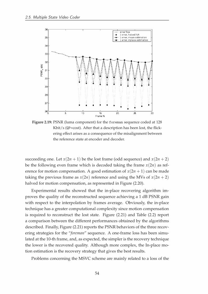
2.5. Multiple State Video Coder
Figure 2.19: PSNR (luma component) for the foreman sequence coded at 128
Kbit/s (QP=cost). After that a description has been lost, the flick-
ering effect arises as a consequence of the misalignment between
the reference state at encoder and decoder.
succeeding one. Let x(2n + 1) be the lost frame (odd sequence) and x(2n + 2)
be the following even frame which is decoded taking the frame x(2n) as ref-
erence for motion compensation. A good estimation of x(2n + 1) can be made
taking the previous frame as x(2n) reference and using the MVs of x(2n + 2)
halved for motion compensation, as represented in Figure (2.20).
Experimental results showed that the in-place recovering algorithm im-
proves the quality of the reconstructed sequence achieving a 1 dB PSNR gain
with respect to the interpolation by frames average. Obviously, the in-place
technique has a greater computational complexity since motion compensation
is required to reconstruct the lost state. Figure (2.21) and Table (2.2) report
a comparison between the different performances obtained by the algorithms
described. Finally, Figure (2.21) reports the PSNR behaviors of the three recov-
ering strategies for the “foreman” sequence. A one-frame loss has been simu-
lated at the 10-th frame, and, as expected, the simpler is the recovery technique
the lower is the recovered quality. Although more complex, the In-place mo-
tion estimation is the recovery strategy that gives the best results.
Problems concerning the MSVC scheme are mainly related to a loss of the
54

2.5. Multiple State Video Coder
x(2n) x(2n+2)x(2n+1)
(lost frame)
even−subsequencemotion vector
odd−subsequeceestimated motion vector
(received frame)(received frame)
Figure 2.20: Error-concealment using in-place motion compensation. The mo-
tion vector of the lost frame x(2n + 1) is reconstructed halving the
motion vector of the frame x(2n + 2).
0 10 20 30 40 50 60 70 80 90 10024
26
28
30
32
34
36
38
40
42
44
PS
NR
Y (
db)
Frame N.
no errors1 error, halved frame rate1 error, average1 error, inplace−MC
Figure 2.21: PSNR (luma component) of the odd frames for the “foreman”
sequence coded at 128 Kbit/s (QP=cost) using different error-
concealment techniques. In-place motion estimation outperforms
the halved-frame rate and the average methods, but is more compu-
tational demanding.
55
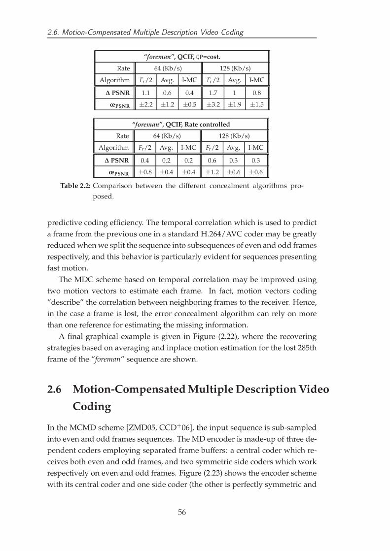
2.6. Motion-Compensated Multiple Description Video Coding
“foreman”, QCIF, QP=cost.
Rate 64 (Kb/s) 128 (Kb/s)
Algorithm Fr/2 Avg. I-MC Fr/2 Avg. I-MC
∆ PSNR 1.1 0.6 0.4 1.7 1 0.8
œPSNR ±2.2 ±1.2 ±0.5 ±3.2 ±1.9 ±1.5
“foreman”, QCIF, Rate controlled
Rate 64 (Kb/s) 128 (Kb/s)
Algorithm Fr/2 Avg. I-MC Fr/2 Avg. I-MC
∆ PSNR 0.4 0.2 0.2 0.6 0.3 0.3
œPSNR ±0.8 ±0.4 ±0.4 ±1.2 ±0.6 ±0.6
Table 2.2: Comparison between the different concealment algorithms pro-
posed.
predictive coding efficiency. The temporal correlation which is used to predict
a frame from the previous one in a standard H.264/AVC coder may be greatly
reduced when we split the sequence into subsequences of even and odd frames
respectively, and this behavior is particularly evident for sequences presenting
fast motion.
The MDC scheme based on temporal correlation may be improved using
two motion vectors to estimate each frame. In fact, motion vectors coding
“describe” the correlation between neighboring frames to the receiver. Hence,
in the case a frame is lost, the error concealment algorithm can rely on more
than one reference for estimating the missing information.
A final graphical example is given in Figure (2.22), where the recovering
strategies based on averaging and inplace motion estimation for the lost 285th
frame of the “foreman” sequence are shown.
2.6 Motion-Compensated Multiple Description Video
Coding
In the MCMD scheme [ZMD05, CCD+06], the input sequence is sub-sampled
into even and odd frames sequences. The MD encoder is made-up of three de-
pendent coders employing separated frame buffers: a central coder which re-
ceives both even and odd frames, and two symmetric side coders which work
respectively on even and odd frames. Figure (2.23) shows the encoder scheme
with its central coder and one side coder (the other is perfectly symmetric and
56

2.6. Motion-Compensated Multiple Description Video Coding
(a) (b)
(c)
Figure 2.22: MSVC transmission example. In (2.22(a)) the correctly received
285th frame of the “foreman” sequence is shown, while in the
other two figures the reconstruction of the lost frame is shown.
In (2.22(b)) the frame estimated as mean of the two adjacent cor-
rectly received frames is shown, while in (2.22(c)) the inplace mo-
tion compensation is adopted. It clearly appears that the solu-
tion based on averaging frames leads to ghosting artifacts, while
inplace motion compensation leads to blocking artifacts, due to
motion estimation and lack of the residual signal.
57

2.6. Motion-Compensated Multiple Description Video Coding
therefore has not been reported).
Let QP0 and QP1 be, respectively, the quantization parameters of central
coder and side coders. The value set for QP0 defines the total amount of full-
rate distortion D0 admitted in case of correct transmission. Usually, this is
a fixed parameter of the system design. Instead, QP1 controls the distortion
introduced when only one description arrives, and determines the capabilities
of the MCMD decoder to reconstruct the lost reference state from only one
description. The smaller is QP1, the greater is the efficiency of side coders to
approximate the correct reference state.
The central coder works on the full-rate sequence, and predicts the current
frame x(n) from the previous two, x(n − 1) and x(n − 2), by implementing
a second-order linear predictor after the block-based motion compensation in
the DPCM loop (MC block) as shown in Figure (2.23).
x0(n) = a1 x0(n − 1) + (1 − a1)x0(n − 2) . (2.3)
The coefficient a1 ∈ [0, 1] in (2.3) controls the trade-off between coding effi-
ciency and robustness to channel errors. The central prediction error
e0(n) = x(n) − x0(n) (2.4)
is quantized (Q0 block in Figure (2.23) using the quantization step QP0, and
yields the output signal
e0(n) = e0(n) + q0(n) = x(n) − x0(n) + q0(n) (2.5)
where q0(n) is the quantization error under the assumption of granular distor-
tion.
Side coders are two standard-compliant H.264 encoders which process ei-
ther even or odd frames, respectively. Let x(2k) be the even frame sequence
and x(2k + 1) the odd one, then the error signals processed by side coders are
e1(n) = e∗1(n) − e0(n) i f n = 2k, k ∈ N
e2(n) = e∗2(n) − e0(n) i f n = 2k + 1, k ∈ N(2.6)
where the signals e∗1(n) and e∗2(n) are given by
e∗1(n) = x(n) − x1(n − 2) i f n = 2k, k ∈ N
e∗2(n) = x(n) − x2(n − 2) i f n = 2k + 1, k ∈ N .(2.7)
58
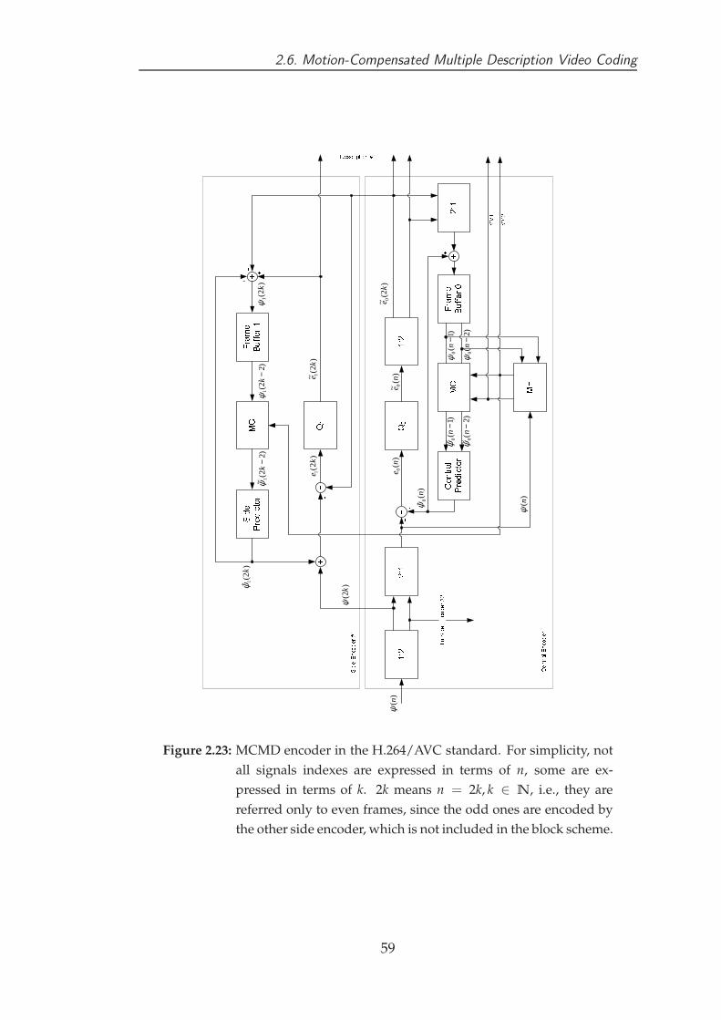
2.6. Motion-Compensated Multiple Description Video Coding
� ��� ��� � � ��� � � � � �� �
� �� � ��� ��� ���� ��
� �� � ��� ��� �
�� � � � � �� � ���
�
� ���� � !"�� �#$%)
(nψ
)2(k
ψ
)2(
ˆ 1k
ψ
)2(
1k
ψ
)2(
1k
e)
2(~ 1
ke
)(
0n
e)
(~ 0
ne
)2(
~ 0k
e
)1(
~ 0−
nψ
)(
ˆ 0n
ψ
&'( )* +,-( )./0 1 )+2 .34* +,-( ).
5 6 7 8 9 : ; < : = > ? @A A A
AA
BB A B
A ACD CE
)2(
~ 0−
nψ
)1(
0−
nψ
)2(
0−
nψ
FG0 FGH
CD
)22(
~ 1−
kψ
)22(
1−
kψ
)(n
ψ
Figure 2.23: MCMD encoder in the H.264/AVC standard. For simplicity, not
all signals indexes are expressed in terms of n, some are ex-
pressed in terms of k. 2k means n = 2k, k ∈ N, i.e., they are
referred only to even frames, since the odd ones are encoded by
the other side encoder, which is not included in the block scheme.
59

2.6. Motion-Compensated Multiple Description Video Coding
After the signals e1(2k) and e2(2k + 1) are quantized with quantization step
QP1, a distortion signal is added producing
e1(n) = e1(n) + q1(n) (2.8)
e2(n) = e2(n) + q2(n) . (2.9)
It can be easily verified that the following relationships hold
e1(n) = x0(n) − x1(n) (2.10)
e2(n) = x0(n) − x2(n) . (2.11)
In the original MCMD scheme, motion estimation is performed only once
in the central coder for the two reference frames x(n− 1) and x(n− 2) yielding
the two sets of motion vectors MV1 and MV2. On the other hand, side coders
have no motion estimation, and use the vectors MV2 computed by the central
coder for their motion compensation. Since motion-vectors number and val-
ues are necessarily associated to the current partitioning of macroblocks, side
coders are forced to take the same macroblock layout of the central coder. This
constraint is highly inefficient since side coders must have QP1 larger than
QP0, and this fact decreases the quality of their reference frames. Constrain-
ing a finer side partition increases the bit-rates required to code side motion
vectors, and reduces the control over the redundancy allocated in the system.
In the H.263 standard, a constrained side macroblock layout does not affect
significantly the MCMD performance since only two types of partitioning are
used. Instead, the new coding features of H.264/AVC permit to partition a
macroblock down to 4× 4 sub-blocks. This fact increases the number of differ-
ent blocks layouts and motion vectors displacements. As a consequence, the
resulting side coding bitrates greatly vary according to how the partitioning
has been chosen.
In order to bound the increment of redundancy in the H.264/AVC stan-
dard, an advanced three-steps motion estimation algorithm was implemented.
Forcing the macroblock partition at side coders increases the additional re-
dundancy. In order to mitigate this effect, we let each side coder to estimate
independently its optimal motion vectors and macroblock partitions. Unfor-
tunately, the reconstructed frame at the central coder is not yet available, and
therefore, side coders cannot coherently perform motion compensation and
provide their mismatch signal. However, under the reasonable hypothesis that
the mismatch signal contains mainly high-frequency components, we may as-
sume that the coarse quantization of side coders retains only low-frequency
60

2.6. Motion-Compensated Multiple Description Video Coding
components, allowing us to perform side motion estimation before the central
one. The resulting algorithm can be summarized in the following three steps.
1. The motion vectors MV2 and macroblock partitions for side coders are
estimated.
2. The MV2 set is passed to the central coder, and central motion estimate is
performed by computing the MV1 set. Since this operation may imply a
different optimal macroblock layout, the MV2 vectors need to be adapted
to fit it. Adaptation is obtained by splitting the blocks used for motion
estimation in the side encoder and replicating the partitioning structure
of the central encoder.
3. The mismatch signal is computed as the difference between the recon-
structed frames at central and side coders, see Equation (2.6). No motion
estimation is performed in this step.
Following this three-step algorithm, the estimate of the MV2 motion vectors
is demanded to side coders rather than the central one. Thus, side bit-rates sig-
nificantly decrease at the expense of using sub-optimal MV2 motion vectors in
the central coder. Nevertheless, simulations showed that the resulting overall
redundancy is acceptable for MDC applications.
Forcing side coders to compute the MV2 motion vectors instead of the cen-
tral coder yields a great decrement of side coders bit-rates, at the cost of non-
optimal motion vectors used in the central coder. Nevertheless, the resulting
overall redundancy is now acceptable for MCMD applications as simulations
showed.
The main characteristic of this MDC scheme is its closed-loop structure,
which makes possible to control the decoder drift in case of transmission error.
Unfortunately, this approach has two drawbacks that pose a serious limitation
on its adoption. First, it is extremely heavy: simulations require very long
times, because every operation in the encoder is doubled. Therefore, it is im-
possible to use it on mobile devices, which will not be able to execute it in an
acceptable time because of lack of sufficient computational resources. Second,
the drift control is slow. Even in case it could run in real-time, the same effect
could be achieved by refreshing the decoder status, either by transmitting an
Intra frame or by adopting intra-refreshing, which has the main advantage of
not increasing the required bandwidth at the cost of requiring longer time to
refresh the full decoder status.
61

2.7. MDSQ-based Multiple Description Video Coding
0 10 20 30 40 50 60 70 80 90 10022
24
26
28
30
32
34
36
38
Frame number (n)
PS
NR
y (dB
)
PSNR after a description loss (at frame 11) Sequence Foreman − (QP
0=29, QP
1=42)
a1=0.1
a1=0.5
a1=0.9
no errors
Figure 2.24: Transmission example for the “foreman” sequence with QP0 = 29
and QP1 = 42, in case of transmission error at the eleventh frame.
The PSNR is plotted for three values of the a1 parameter, i.e. the
weights of the second order predictor.
A final graphical example of error recovery with MCMDC for the “foreman”
sequence is given in Figure (2.25), where the estimated frame and the error are
shown.
2.7 MDSQ-based Multiple Description Video Cod-
ing
2.7.1 The Multiple Description Scalar Quantizer
The Multiple Description Scalar Quantizer [Vai93b] (MDSQ) is an extension
of the optimal Lloyd-Max Scalar Quantizer (SQ), where the encoder sends the
information over two different channels subject to a rate constraint.
Formally, let x be the output of a random process we want to encode. Sup-
pose that the transmission system has two channels with transmission rates R1
and R2, that may be in a working or non-working state.
An (M1, M2)-level MDSQ maps source samples x onto the reconstruction
levels
x0 ∈ X 0 ={
x0ij, (i, j) ∈ C
}
(2.12)
62

2.7. MDSQ-based Multiple Description Video Coding
(a)
(b)
(c)
Figure 2.25: MCMDC transmission example of the “foreman” sequence.
In (2.25(a)) the correctly received frame is shown. Figure (2.25(b))
holds the reconstructed frame in case of transmission error and
Figure (2.25(c)) shows the difference of the two previous frames.
63
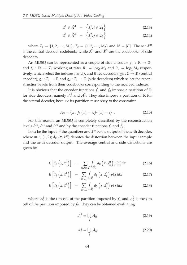
2.7. MDSQ-based Multiple Description Video Coding
x1 ∈ X 1 ={
x1i , i ∈ I1
}
(2.13)
x2 ∈ X 2 ={
x2j , j ∈ I2
}
(2.14)
where I1 = {1, 2, · · · , M1}, I2 = {1, 2, · · · , M2} and N = |C|. The set X 0
is the central decoder codebook, while X 1 and X 2 are the codebooks of side
decoders.
An MDSQ can be represented as a couple of side encoders f1 : R → I1
and f2 : R → I2 working at rates R1 = log2 M1 and R2 = log2 M2 respec-
tively, which select the indexes i and j, and three decoders, g0 : C → R (central
encoder), g1 : I1 → R and g2 : I1 → R (side decoders) which select the recon-
struction levels from their codebooks corresponding to the received indexes.
It is obvious that the encoder functions f1 and f2 impose a partition of R
for side decoders, namely A1 and A2. They also impose a partition of R for
the central decoder, because its partition must obey to the constraint
Aij = {x : f1 (x) = i, f2 (x) = j} . (2.15)
For this reason, an MDSQ is completely described by the reconstruction
levels X 0, X 1 and X 2 and by the encoder functions f1 and f2.
Let x be the input of the quantizer and xm be the output of the m-th decoder,
where m ∈ (1, 2); dm (x, xm) denotes the distortion between the input sample
and the m-th decoder output. The average central and side distortions are
given by
E[
d0
(
x, x0)]
= ∑(i,j)∈C
∫
Aij
d0
(
x, x0ij
)
p(x)dx (2.16)
E[
d1
(
x, x1)]
= ∑i∈I1
∫
A1i
d1
(
x, x1i
)
p(x)dx (2.17)
E[
d2
(
x, x2)]
= ∑j∈I2
∫
A2j
d2
(
x, x2j
)
p(x)dx (2.18)
where A1i is the i-th cell of the partition imposed by f1 and A2
j is the j-th
cell of the partition imposed by f2. They can be obtained evaluating
A1i =
⋃
j
Aij (2.19)
A2j =
⋃
i
Aij (2.20)
64

2.7. MDSQ-based Multiple Description Video Coding
For given values M1, M2, D1, D2, an MDSQ is said to be optimal if it solves
the following minimization problem:
min E [d0]
E [d1] ≤ D1
E [d2] ≤ D2
(2.21)
In case M1 = M2, the MDSQ is said to be balanced if E [d1] = E [d2].
Computing optimal reconstruction levels for a MDSQ is connected to the
index assignment problem. Since A1i and A2
j are tied to Aij by (2.19) and (2.20),
it easy to understand that indexes ij of the central decoder cells impose the
shape of side decoders cells and affect side decoders performance. Vaisham-
payan proposed two different algorithms to solve this problem, namely the
nested index assignment and the linear index assignment. Both algorithms scan
the encoders cells as if they were matrix elements lying on the main and its 2k
neighbor diagonals and associate a progressive number with them. Since each
matrix element is associated to a couple of indexes, the scanning algorithms
map the central decoder cells indexes to those of the side decoders.
The nested index assignment scans the matrix elements in two ways: the east
scan and the south scan, which always start from an element of the matrix
main diagonal. The east scan starting from element of index (i, i) is given by
the sequence (i, i), (i, i + 1), (i + 1, i), (i, i + 2), (i + 2, i), · · · , (i, i + k), (i + k, i)
and the south scan is represented by the sequence (i, i), (i + 1, i), (i, i + 1),
(i + 2, i), (i, i + 2), · · · , (i + k, i), (i, i + k). In order to obtain two balanced de-
scription, these two scanning strategies are pairwise alternately applied.
The linear index assignment also consists of two different scan types, namely
the U-scan and the D-scan, which are alternately applied as those of the nested
index assignment. These methods start from an element of one of the most ex-
ternal diagonals, scan the matrix elements orthogonally to the main diagonal
and finish when they reach the opposite external diagonal. Each scan can hold
an even or odd number of elements. In case this number is odd, the U and D
scans are described by the sequences(
i +⌊
k2
⌋
, i −⌊
k2
⌋)
,(
i +⌊
k2
⌋
− 1, i −⌊
k2
⌋
+ 1)
, · · · ,(
i −⌊
k2
⌋
, i +⌊
k2
⌋)
and(
i −⌊
k2
⌋
, i +⌊
k2
⌋)
,(
i −⌊
k2
⌋
+ 1, i +⌊
k2
⌋
− 1)
, · · · ,(
i +⌊
k2
⌋
, i −⌊
k2
⌋)
respectively, while a simi-
lar expression can be obtained for an odd number of cells.
It can be shown that varying the value of k and therefore altering the num-
ber of diagonals used in the scanning process, the behavior of side decoders
changes. For small values of k, side decoders work at high bitrate and low
distortion, while for big values of k their quality decreases together with the
65

2.7. MDSQ-based Multiple Description Video Coding
bitrate associated with them.
2.7.2 Implementation of the scheme
We decided to implement a MDSQ based scheme on the JVT H.264/AVC ref-
erence code using the base layer with the addiction of B frames and imposing
some constraints on its design:
1. the central decoder must reconstruct the same sequence as if it were a
standard single description encoder;
2. both descriptions have to be singularly decodable by a standard decoder
and;
3. the introduced computational overhead should be kept as small as pos-
sible.
All these goals were achieved inserting a splitting block in the standard
H.264/AVC scheme after quantization, as show in Figure (2.26). This block
generates two descriptions duplicating the control structures like SPS, PPS and
SH and information about the motion vectors. Before passing the residual in-
formation to the Network Abstraction Layer (NAL), coefficients are divided
into two descriptions applying a MDSQ. Since the quantization pass is stored
in several places (PPS, SH and the macroblock layer), we decided to set the
same QP value in the central and side decoders. This non optimal solution re-
duces the computational overhead but at the same time increases distortion
in the side decoders. As subsequently explained, this is not a great problem,
because total distortion does not increases too much: DCT coefficients follow
a laplacian-like p.d.f. and small values distortion is small.
The decoder can be implemented similarly to the encoder. A merge block
has to be added between the NAL and the inverse quantizer. Whenever the
decoder receives both descriptions, the original quantized value is obtained
from the assignment matrix, while, in case of a channel malfunctioning, the
received description identifies the cell of a side decoder and the H.264/AVC
decoder works as if it were using a bigger QP value. In fact, since many central
decoder cells are mapped into the same side decoder index, we obtain the same
result as if we would obtain quantizing with a larger QP.
The first implementation of the linear index assignment was mainly based
on the algorithm proposed by Vaishampayan in [Vai93b]. The only difference
consisted in assigning the zero value to the center of the assignment matrix
66
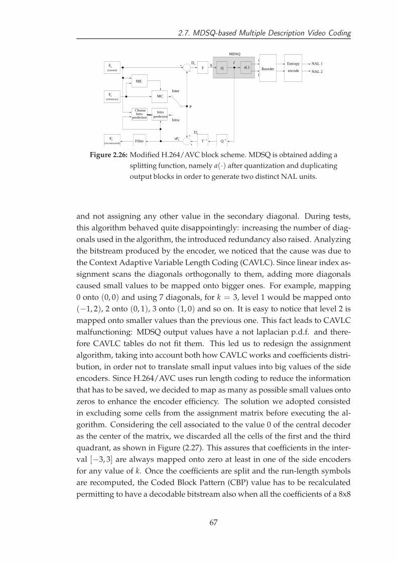
2.7. MDSQ-based Multiple Description Video Coding
Dn’
nDT Q
T −1 Q−1
a(.) ReorderEntropy
encodeFn
n
nF
F ’
’ Fn’u
(current)
(reference)
(reconstructed)Filter
ME
ChooseIntra
prediction
Intraprediction
MC
Intra
Inter
P
+
+
−
+ Xl
MDSQ
j
iNAL 1
NAL 2
Figure 2.26: Modified H.264/AVC block scheme. MDSQ is obtained adding a
splitting function, namely a(·) after quantization and duplicating
output blocks in order to generate two distinct NAL units.
and not assigning any other value in the secondary diagonal. During tests,
this algorithm behaved quite disappointingly: increasing the number of diag-
onals used in the algorithm, the introduced redundancy also raised. Analyzing
the bitstream produced by the encoder, we noticed that the cause was due to
the Context Adaptive Variable Length Coding (CAVLC). Since linear index as-
signment scans the diagonals orthogonally to them, adding more diagonals
caused small values to be mapped onto bigger ones. For example, mapping
0 onto (0, 0) and using 7 diagonals, for k = 3, level 1 would be mapped onto
(−1, 2), 2 onto (0, 1), 3 onto (1, 0) and so on. It is easy to notice that level 2 is
mapped onto smaller values than the previous one. This fact leads to CAVLC
malfunctioning: MDSQ output values have a not laplacian p.d.f. and there-
fore CAVLC tables do not fit them. This led us to redesign the assignment
algorithm, taking into account both how CAVLC works and coefficients distri-
bution, in order not to translate small input values into big values of the side
encoders. Since H.264/AVC uses run length coding to reduce the information
that has to be saved, we decided to map as many as possible small values onto
zeros to enhance the encoder efficiency. The solution we adopted consisted
in excluding some cells from the assignment matrix before executing the al-
gorithm. Considering the cell associated to the value 0 of the central decoder
as the center of the matrix, we discarded all the cells of the first and the third
quadrant, as shown in Figure (2.27). This assures that coefficients in the inter-
val [−3, 3] are always mapped onto zero at least in one of the side encoders
for any value of k. Once the coefficients are split and the run-length symbols
are recomputed, the Coded Block Pattern (CBP) value has to be recalculated
permitting to have a decodable bitstream also when all the coefficients of a 8x8
67

2.7. MDSQ-based Multiple Description Video Coding
2
1
0
−1
−2
−3
−4
−5
5
4
3
−5 −4 −3 −2 −1 0 54321
0−1
−2
−3
−4
−5
−6
−7
−8
−9
−10
−11
−12
−13
−14
−15
−16
−17
−18
−19−25
1
2
3
4
5
6
7
8
9
10
11
12
13
14
15
16
17
18
19
25
20
21
22
23
24
26
−23
−22
−21
−20
−26
−24
U block
D block
Main diagonal
Side
qua
ntiz
er 1
Side quantizer 2
Figure 2.27: Linear index assignment matrix with k = 3 diagonals. The cell
numbers represent the scanning order, the axis show the output
of the side quantizer. The gray blocks show the invalid quadrants
of the matrix.
block have become null after the splitting process.
The nested index assignment was similarly implemented, discarding the
cells of the first and third quadrants of the matrix, because it presented the
same problem with CAVLC. Two new scanning techniques were added, namely
north and west scan, which are symmetrical to south and east scans. These
new scans are used in second quadrant, while those proposed by Vaisham-
payan are adopted for the fourth quadrant.
Figure (2.28) shows that for both methods the redundancy increases with
the value of QP. This happens because for low QP values the bitstream mainly
consists of high-valued residual coefficients, while for high values of QP mo-
tion vectors take most of the bitstream and coefficients have nearly null values.
Therefore in the first case the splitting process is very efficient because, al-
though motion vectors are doubled, they do not require too many bits if com-
pared to the residual information and big coefficients are efficiently mapped
onto small values that can be efficiently represented by the CAVLC. This does
not happen in the second case: motion vectors require a lot of bits when they
68

2.7. MDSQ-based Multiple Description Video Coding
0 20 40
20
30
40
50
60
70
80
QP
Red
unda
ncy
(%)
linear k=1linear k=2linear k=3linear k=4
0 20 40
20
30
40
50
60
70
80
QP
Red
unda
ncy
(%)
nested k=1nested k=2nested k=3nested k=4
Figure 2.28: Introduced redundancy varying the encoder QP for linear (on the
left) and nested (on the right) index assignment method for the
CIF sequence “mobile”. Adding more diagonals to the assignment
matrix, both the methods saturate for k ≥ 2.
are doubled and the splitting process maps low coefficients onto small values
and it is not possible to reduce the required bits.
It is also notable that the introduced redundancy reduces until saturation
is reached. Adding more diagonals makes more values to be mapped onto 0
level. This can improve compression gain because zeros are efficiently encoded
by the run-length coding, but increasing the number of diagonals (k greater
than 2) does not improve compression any more. This is due to the laplacian
distribution of the coefficients. Even though more values are mapped onto 0,
these values are hardly ever used because they are too big and therefore rare.
To simulate a transmission error, we decided to lose a whole frame descrip-
tion. This pessimistic assumption does not occur in real transmission systems.
Big frames are usually divided into slices and error bursts or packets loss do
not damage the whole image. Being aware of this fact, we chose this loss as a
worst case. The corrupted packets belong to the 20th frame, which is a P frame
(B frames are not used for motion compensation, therefore errors in B frames
do not propagate through the decoded sequence).
69
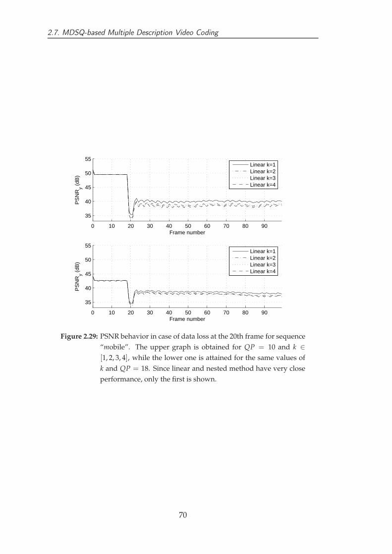
2.7. MDSQ-based Multiple Description Video Coding
0 10 20 30 40 50 60 70 80 90
35
40
45
50
55
Frame number
PS
NR
y (dB
)
Linear k=1Linear k=2Linear k=3Linear k=4
0 10 20 30 40 50 60 70 80 90
35
40
45
50
55
Frame number
PS
NR
y (dB
)
Linear k=1Linear k=2Linear k=3Linear k=4
Figure 2.29: PSNR behavior in case of data loss at the 20th frame for sequence
“mobile”. The upper graph is obtained for QP = 10 and k ∈[1, 2, 3, 4], while the lower one is attained for the same values of
k and QP = 18. Since linear and nested method have very close
performance, only the first is shown.
70

2.8. Performance comparison of the proposed schemes
During the tests, linear and nested assignment methods gave very similar
results, and only for high values of QP and k = 1 the nested index assignment
outperformed the linear one by 0.5 dB. Hence, Figure (2.29) shows the PSNR
behavior only in the linear index assignment case for QP = 10 and QP = 18.
As expected, increasing the number of diagonals the distortion produced by
a description loss becomes always higher because the greater is the number
of diagonals, the smaller is the redundancy between the descriptions. The
proposed scheme has some ability to recover between 4 and 5 dB of PSNR
after information loss. Although this might seem to be a small gain, the visual
quality of the reconstructed scene is good. In many tests we ran, it was not
trivial to identify at sight the difference between correct and the corrupted
frames and we had to calculate the difference of the frames and to enhance it
in order to notice the errors.
Compared with other MDC solutions proposed for the H.264/AVC en-
coder [CCD+06], the proposed scheme is able to give better objective and sub-
jective quality requiring slightly more redundancy.
An example of the quality of the reconstructed frame is given in Figure (2.30)
for QP = 12 and K = 8, where the correctly decoded frame, the reconstructed
frame in case of transmission error and the difference are shown.
2.8 Performance comparison of the proposed schemes
2.8.1 Schemes comparison
Evaluating a MDC scheme is a complex task, because many aspects should be
considered. The Redundancy Rate-Distortion (RRD) region ρ(D1, D0), which
describes the distortion D1 achievable by side decoders as a function of the
allocated redundancy, and with fixed central encoder distortion D0, is often
used to evaluate the capabilities of MDC schemes. The RRD region compari-
son of the explained solutions is proposed. However, it should be noted that it
does not fit particularly well for the coding schemes where redundancy is not
a degree of freedom.
Observe that, in SMDC, MDMC and MSVC the user can not set the amount
of introduced redundancy, since it is an inner property of the encoded se-
quence and not a degree of freedom. In the MCMD and MDSQ-based coding
schemes, instead, redundancy can be varied tuning the side encoders rates.
For this reason, the RRD region is represented by a curve for these two cod-
ing schemes, while it degenerates to a single point for the first three schemes.
71

2.8. Performance comparison of the proposed schemes
(a)
(b)
(c)
Figure 2.30: Transmission example of the “foreman” sequence. In (2.30(a)) the
correctly received frame is shown, while in (2.30(b)) the recon-
structed frame in case of error is shown. Figure (2.30(c)) holds
the difference between the two frames.
72

2.8. Performance comparison of the proposed schemes
10 20 30 40 50 60 7022
24
26
28
30
32
34
36
38
40
Redundancy
PS
NR
dB
MCMD foreman
MDMC foreman
SMDC foreman
MSVC foreman
MDSQ−based foreman
MCMD akiyo
MDMC akiyo
SMDC akiyo
MSVC akiyo
MDSQ−based akiyo
Figure 2.31: Redundancy Rate-Distortion (RRD) regions for the five MD cod-
ing schemes for the “foreman” and “akiyo” QCIF sequences and
QP = 29, in case of a whole frame loss.
In Figure (2.31), the five RRD regions have been reported. These results cor-
respond to the coding of the “foreman” and “akiyo” QCIF sequences using QP
= 29, and assuming that one whole frame is lost during the transmission of a
description.
Figure (2.31) shows the behavior of the proposed schemes related to the
motion complexity of sequences. In this test, “foreman” is a fast-varying se-
quence and “akiyo” is a quasi-static one. The SMCD and MCMD techniques are
substantially invariant to the characteristics of the scene being encoded. On the
contrary, the MDMC, the MDSQ-based and the MSVC algorithms are strongly
affected by the amount of motion: MDMC performs well with non-static se-
quences because the produced bitstream principally consists of the residual
information that is not doubled in the splitting process, while the estimate of
the lost state in SMCD works at its best on static scenes.
Since PSNR is not the only relevant aspect, but also computational cost and
syntax compliance are important, we propose the qualitative comparison of
the considered schemes, which is reported in Table (2.3).
73

2.8. Performance comparison of the proposed schemes
SMDC MDMC MSVC MCMD MDSQ
Exploited correlation spatial spatial temporal temporal quantization
Efficiency good good quite good variable variable
Computational Cost medium low medium high low
Syntax Compliance yes yes yes no yes
Tunability no no no yes yes
Table 2.3: Qualitative comparison of the considered MD coding techniques.
Spatial MDC schemes usually demand lower computational complexity
than temporal ones. In fact, in temporal MDC algorithms the storage of many
reference frames is required, and in the particular case of the MCMD algo-
rithm, there is also an extra computational load due to the double motion es-
timation required to compute two motion vectors fields. In the MCMD, as
for the MSVC, the number of operations is roughly the same of a standard
H.264/AVC encoder. However, it requires a double-sized frame buffer. from
the computational point of view, MDMC is the lightest solution, because is doe
We must also point out that MSVC, SMDC, MDMC provide fully
H.264/AVC-compliant bitstreams which can be, thus, decoded by a standard
H.264/AVC decoder. MCMD streams do not correspond to the standard
H.264/AVC syntax, and require an ad-hoc multiple-description decoder at the
receiver. In addition, we must also observe that the MDMC layer is external to
the H.264/AVC core unit, and can be independently developed and optimized
since it only depends on the bitstream syntax.
74
Chapter 3
Scalable Video Coding
3.1 Introduction to Scalable Video Coding
Scalable video coding [Ohm05] allows reconstruction of lower resolution, lower
framerate or lower quality sequences from partially received bitstream. Thus,
the stream can be dynamically adapted to the network conditions. Moreover,
media contents distribution is not going to be bounded only to DVDs, but it
is going to be supported by networking applications based both on wireless
LANs and cable networks, such as p2p video.
Additionally, video sequences are going to be viewed on several different
types of devices, ranging from small handheld devices such as mobile phones
or PDAs to widescreen high definition displays. Different networks character-
istics, together with all the possible displays, originate a huge set of distinct
scenarios that a modern video codec has to be able to deal with.
Scalable video codecs encode the input signal once at highest quality, but
allow partial decoding of the compressed information by the user decoder.
Thus, flexible transmission over heterogeneous networks and optimal decod-
ing under the constraints imposed by the user hardware limitation are possi-
ble. Scalability is usually achieved in three dimensions: spatial resolution, to
adapt the encoded sequence to several screens sizes, temporal resolution, to
decode the bitstream at the maximum speed allowed by the computational re-
sources of the display and quality-level resolution, which is often referred to
as SNR scalability, to match network bandwidth.
In popular motion-compensated prediction and block coding algorithms,
inefficiency rises when they are adapted to provide such scalability. The most
critical cause of this performance drop is given by the prediction loop. In fact,
as soon as some information is lost, the reference frames at the encoder and
decoder are no longer the same, and the reconstructed sequence diverges from
75
3.1. Introduction to Scalable Video Coding
the reconstructed signal at the encoder used in the closed loop prediction. In
the last years, several breakthroughs both in wavelets but also in hybrid video
codecs have brought to the proposal of efficient scalable video codecs. As for
the JPEG2000 image coding standard [TM02], wavelets can provide spatial and
temporal scalability, while innovations in hybrid codec have been applied to
the Joint Scalable Video Model (JSVM) [RWS05].
3.1.1 Scalability in existing coding standards
The standards IUT-T H.261 [Rec90] and ISO/IEC MPEG-1 [SR] did not pro-
vide any kind of scalability at the time they were defined, because they were
designated for very specific applications such as video conference over chan-
nels characterized by a fixed bandwidth or storage. The only possible solution
to provide scalability is the so called simulcast, where two or more streams re-
lated to the same sequence but encoded at different qualities are transmitted
together on the network. Simulcast is the most inefficient solution for scala-
bility, since it requires independent compressions of the input signal, without
being able to exploit the intrinsic redundancy.
Simulcast is also available in ISO/IEC MPEG-2 [EF95], which maintains
backward compatibility towards MPEG-1 in order to allow the low-quality
stream to be encoded by using MPEG-1 and the high-quality sequences to be
encoded with the new standard. MPEG-2 introduced also another tool to pro-
vide scalability in the Main+ and Next profiles, based on layered coding, where
some refinement layers can be added to the low-quality sequence to enhance
the quality of the decoded video. Obviously, in case the low-quality sequence
is not correctly received and decoded, no information can be extracted from
the enhancement layers, which depend on it. The MPEG-2 video scalability
modes can be summarized as:
• Spatial scalability: useful in simulcasting, and for feasible software de-
coding of the lower resolution, base layer. This spatial domain method
codes a base layer at lower sampling dimensions (i.e. "resolution") than
the upper layers. The up-sampled reconstructed lower (base) layers are
then used as prediction for the higher layers.
• SNR scalability: similar to the point transform in JPEG, SNR scalability
is a spatial domain method where channels are coded at identical sam-
ple rates, but with differing picture qualities (through quantization step
sizes). The higher priority bitstream contains a base layer data that can be
76

3.1. Introduction to Scalable Video Coding
added to a lower priority refinement layer to construct a higher quality
picture.
• Temporal scalability: the first, higher priority bitstream holds a video at
a lower frame rate, and the intermediate frames can be coded in a second
bitstream using the first bitstream reconstruction as prediction. As an
example, in stereoscopic vision the left video channel can be predicted
from the right channel.
• Data partitioning: it is similar to frequency progressive mode of
JPEG [DIS91], where the slice layer indicates the maximum number of
block transform coefficients contained in the particular bitstream (known
as the "priority break point"). Data partitioning is a frequency domain
method that breaks the block of 64 quantized transform coefficients into
two bitstreams. The first, higher priority bitstream contains the more crit-
ical lower frequency coefficients and side informations (such as DC val-
ues, motion vectors). The second, lower priority bitstream carries higher
frequency AC data.
Frequency scalability was also proposed for the MPEG-2 standard, but it
was dropped because of its complexity and not excellent quality.
The MPEG-4 [Ric03] standard has similar tools, which are organized in a
more flexible framework at the level of Video Objects (VO), i.e. areas of the
video scene that may occupy an arbitrarily-shaped region and may exist for an
arbitrary length of time. An instance of a VO at a particular point in time is a
Video Object Plane (VOP). This definition encompasses the traditional approach
of coding complete frames, in which each VOP is a single frame of video and a
sequence of frames forms a VO. However, the introduction of the VO concept
allows more flexible options for coding video.
In case of spatial scalability, an I-VOP in an enhancement layer is encoded
without any spatial prediction, i.e. as a complete frame or object at the en-
hancement resolution. In an enhancement layer P-VOP, the decoded,
up-sampled base layer VOP at the same position in time is used as a predic-
tion without any motion compensation. The difference between this prediction
and the input frame is encoded using the texture coding tools, i.e. no motion
vectors are transmitted for an enhancement P-VOP. An enhancement layer B-
VOP is predicted from two directions. The backward prediction is formed by
the decoded, up-sampled base layer VOP at the same position in time, with-
out any motion compensation and hence without the motion vector field. The
forward prediction is formed by the previous VOP in the enhancement layer
77

3.1. Introduction to Scalable Video Coding
even if this is itself a B-VOP, with motion-compensated prediction and hence
motion vectors.
In temporal scalability, an enhancement I-VOP is encoded without any pre-
diction. An enhancement P-VOP is predicted from the previous enhancement
VOP, the previous base layer VOP or the next base layer VOP. An enhance-
ment B-VOP is predicted from the previous enhancement and previous base
layer VOPs, the previous enhancement and next base-layer VOPs or the previ-
ous and next base-layer VOPs.
SNR scalability is obtained by adopting Fine Granular Scalability
(FGS) [Li01], which is based on encoding the sequence as a base layer and an
enhancement layer. The enhancement layer is embedded, i.e. it can be truncated
during encoding or during transmission by a bitstream extractor, assuring that
the decoded quality is maximum at any truncation point. A typical applica-
tion example is given by a server streaming the base layer and a part of the en-
hancement layer to the client. The amount of truncation is chosen depending
on network conditions and available bandwidth, thus maximizing the quality
without having to re-encode the input signal.
A final remark has to be given to H.264/AVC. In fact, an SVC amendment
for this standard has been approved [HPCH07], which adds several new tech-
niques to the non-scalable standard:
• hierarchical B structure;
• adaptive interlayer prediction techniques, to exploit correlation between
spatial and SNR coding layers;
• use of the enhancement layer information in the prediction loops;
• Adaptive Reference FGS, which makes use of leaky prediction by select-
ing a leaky factor at transform coefficient level to deal with drifting er-
rors.
The hierarchical B structure, as well as interlayer prediction techniques and
leaky prediction will be successively explained, because they are not only re-
ferred to the H.264/AVC standard.
3.1.2 Wavelets and wavelet-based spatial scalability
The Fourier synthesis theory asserts that a 2π-periodic function f (x) can be
written as
78

3.1. Introduction to Scalable Video Coding
f (x) = a0 +∞
∑k=1
(ak cos kx + bk sin kx) (3.1)
where the coefficients a0, ak and bk are calculated by
a0 =1
2π
∫ 2π
0f (x)dx (3.2)
ak =1
2π
∫ 2π
0f (x) cos(kx)dx (3.3)
bk =1
2π
∫ 2π
0f (x) sin(kx)dx. (3.4)
Successively the Fourier transform has been defined on non-periodic func-
tions, but it does not take into account local information. The first attempt
to deal with not-periodic signal and multi-scale analysis was proposed by ex-
tending the Fourier transform adding a windowing operation, thus obtain-
ing the Windowed Fourier Transform (WFT). In the WFT, the input signal is
chopped into portions, which are independently analyzed for their frequency
contents. The choice of the windows profile influences the analysis quality
because it introduces distortion
F [ f (x) · w(x)] = F [ f (x)] ∗ F [w(x)] . (3.5)
Thus the frequency profile of the signal is convolved with the frequency
response of the window w(x). This leads to reduced resolution, due to the
width of the main lobe of F [w(x)], and spectral leakage, which is related to
the side lobes of the frequency window profile. As an example, the rectangular
window, whose Fourier transform is the sinc function, has the narrowest main
lobe for a given windows length, but it has the largest side lobes of all the
commonly used windows [OS75].
The trade-off between the main and side lobes width can be quantified by
looking for a window function that is maximally concentrated around ω = 0
in the frequency domain. Kaiser [Kai74] proposed a near-optimal solution to
this problem by using a zeroth-order modified Bessel function of the first kind.
The successive step in multiscale frequency analysis, was the proposal of
a new kind of transform, the wavelet transform. Wavelets [Gra95] are mathe-
matical functions that divide the input signal into frequency components and
analyze each component with a resolution matched to its scale. As in many
other other transforms, the input signal is decomposed as the superposition of
basis functions, however in wavelet analysis a very important role is played by
79

3.1. Introduction to Scalable Video Coding
the scale, i.e. the resolution used to inspect the signal. Whenever a small win-
dow is used, small features are examined, while larger windows scan gross
details.
Given a mother function or analyzing wavelet Φ(x), an orthogonal basis can
be defined as
Φ(s,l)(x) = 2−s2 Φ(2−sx − l) , (3.6)
where the variables s and l are integers that scale and dilate the mother
functions Φ to generate the other basis functions. Particularly, s is the index
scale that modifies the wavelets width and l is the location index. Since s and
l are integers, the functions are scaled by powers of two and translated by in-
tegers, so thanks to the self-similarity it is necessary to know only the scaling
function to describe the whole basis. To span the input signal at different reso-
lutions, the analyzing wavelet is used in a scaling equation
W(x) =N−2
∑k=−1
(−1)kck+1Φ(2x + k) , (3.7)
where W(x) is the scaling function for the mother function Φ and ck are the
wavelet coefficients, which have to satisfy linear and quadratic constraints of the
form
N−1
∑k=0
ck = 2 ,N−1
∑k=0
ckck+2l = 2δl,0 . (3.8)
The coefficients {c0, · · · , cn} can be thought as the coefficients of a low-pass
filter. By reversing the taps order and by multiplying them by the sequence
(1,−1, 1,−1, · · · , 1,−1), an high-pass filter is obtained, which has a frequency
response specular to the one of the low-pass filter. The two filters are said to
be quadrature mirror filter pair and enable aliasing-free analysis. A couple of
synthesis filters can be derived by imposing perfect reconstruction, so that the
inverse transform can be realized.
These filters pair is applied several times to the input signal, each time to
the smoothed data: each time they are applied to the low-pass output of the
previous iteration, or to the whole signal in case of the first application, a new
sub-band is created, and part of the frequencies extracted from the input signal,
so that it can be sub-sampled and be fed as low-pass input to the following
step. Clearly, the more filtering operations are performed, the more sub-bands
are available. To each sub-band is associated a spatial resolution of the input
80

3.1. Introduction to Scalable Video Coding
signal, because the inverse transform can be truncated at any sub-band and a
scaled, aliasing-free subsampled version of the original signal is reconstructed.
An example of local analysis with wavelets is shown in Figure (3.1), where
the input signal f (x) = sin(x2) is analyzed with the Daubechies 4 wavelet. The
signal doesn’t have a constant spectral profile, but high frequencies become
more and more important when x increases. Thus, local analysis at values of
x close to 0 shows the predominance of low frequency components, but by
increasing x these elements vanish while high frequencies appear.
Since the wavelet transform is a subband transform, it can be implemented
with a filter bank [Mal89], as shown in Figure (3.2), where the forward trans-
form uses two analysis filters h and g followed by sub-sampling. In reconstruc-
tion after up-sampling the output of two synthesis filters h and g are summed
together to reconstruct the original signal.
To assure perfect reconstruction, two conditions have to be satisfied
{
h(z)h(z−1) + g(z)g(z−1) = 2
h(z)h(−z−1) + g(z)g(−z−1) = 0. (3.9)
When h = h and g = g, {h, g, h, g} forms an orthogonal wavelet transform.
By using the polyphase representation of a filter, h can be written as he(z2) +
z−1ho(z2) where he(z) contains the even coefficients and ho(z) the odd ones.
Thus the filter pair (h, g) can be written with the polyphase matrix P(z) as
P(z) =
[
he(z) ho(z)
ge(z) go(z)
]
(3.10)
and the corresponding transform can be written as
[
r1(z)
d1(z)
]
= P(z)
[
xe(z)
z−1xo(z)
]
(3.11)
Daubechies and Sweldens [DS98] proved that any polyphase matrix repre-
senting a wavelet transform can be decomposed in primal and/or dual lifting
steps by applying the LU decomposition. In these lifting steps, new finite filter
hnew and gnew are respectively evaluated as
hnew(z) = h(z) + s(z2)g(z) (3.12)
and
gnew(z) = g(z) + t(z2)h(z) (3.13)
81

3.1. Introduction to Scalable Video Coding
0 2 4 6 8 10 12−1
−0.5
0
0.5
1Input signal f(x) = sin(x2)
0 10 20 30 40 50 60 70 1
2
3
4
5
0
1
2
3
Local frequency
Absolute value of the DB4 wavelet transform
Position
Figure 3.1: Example of local analysis with wavelet. The DB4 wavelet is used
to analysis the input signal y = sin(x2). Since low frequency
values in the wavelet analysis are shared between high-frequency
samples, it is necessary to interpolated them so that for each po-
sition in the signal domain all frequency values are shown. By
doing this operation a result similar to the windowed DFT is ob-
tained, an it is possible to see how the output of the local transform
varies while the analysis window is shifted. In this case, the sig-
nal y = sin(x2) increases its frequency and the output of the local
analysis with the DB4 wavelet shows how the low frequency com-
ponents decrease and the high-frequencies grow while the analy-
sis window moves along the signal.
h(z)
g(z) 2
2 2
2
h(z )−1~
g(z )−1~
x(z) x(z)
Figure 3.2: Basic filter bank for biorthogonal wavelet transform.
82

3.1. Introduction to Scalable Video Coding
where s(z) and t(z) are Laurent polynomials. Thus the polyphase matrix
can be written as
Pnew(z) =
[
1 s(z)
0 1
]
P(z) or Pnew(z) =
[
1 0
t(z) 1
]
P(z). (3.14)
By alternating these two steps, every polyphase matrix can be decomposed
into the product of several triangular 2× 2 matrixes and a diagonalization ma-
trix. This decomposition has three main advantages:
• it reduces the computational requirements because sk(t) and tk(t) are of-
ten either scalar values or monomials, thus buffers can be reduced;
• since each step depends on the output of the previous stage, pipelining
can be easily adopted to increase output speed;
• the inverse transform can be easily evaluated by inverting the steps and
by swapping the input and output of each lifting step.
In Figure (3.3), the general block scheme of a lifted direct wavelet transform
is shown.
1s (z) s (z)2t (z)1 2t (z)
x o
x e
Figure 3.3: Lifted direct transform block scheme. By inverting the data flow,
the scheme of the inverse transform is obtained.
Wavelets are used in several applications, from physics to engineering. For
image and video coding, 2D and 3D wavelets are used to provide scalability.
Since the wavelet transform consists of a couple of filters which separate low-
and high-frequency components, it can be used for up- and down-sampling.
In fact, by applying an orthonormal transform, the low-pass filtered image can
be down-sampled without aliasing. Similarly, a zero-padded image can be fed
to the inverse transform to obtain an upsampled image. Whenever the inverse
transform is applied not only to the downsampled image but also to the high-
frequency coefficient the original full resolution image is obtained.
83

3.1. Introduction to Scalable Video Coding
An example of wavelet application for image coding is the JPEG2000 [TM02],
where the reversible 5/3 and the non-reversible 9/7 wavelet transforms are
used. The first wavelet is an integer-to-integer [AK00] reversible transform
which guarantees perfect image reconstruction and thus it is used for lossless
image compression. The 9/7 wavelet is a floating point transform, thus there
is some flexibility in its implementation and it is meant to be used for lossy
image coding.
Both transforms can be implemented by using the lifting scheme [AW01].
The 5/3 wavelet can be written as
d[n] = d0[n] +
⌊
1
2(s0[n + 1] + s0[n])
⌋
(3.15)
s[n] = s0[n] +
⌊
1
4(d[n] + d[n − 1]) +
1
2
⌋
. (3.16)
Similarly the 9/7 transform can be decomposed in
d1[n] = d0[n] − α0 (s0[n + 1] + s0[n]) (3.17)
s1[n] = s0[n] − α1 (d1[n] + d1[n − 1]) (3.18)
d2[n] = d1[n] + α2 (s1[n + 1] + s1) (3.19)
s2[n] = s1[n] + α3 (d2[n] + d2[n − 1]) (3.20)
s[n] = β0s2[n] (3.21)
d[n] = β1d2[n] (3.22)
where
α0 ≈ 1.586134, α1 ≈ 0.052980, α2 ≈ 0.882911,
α3 ≈ 0.443506, β0 ≈ 0.812893, β1 = 1/β0.
3.1.3 SNR scalability for predictive coding techniques
The generic block scheme of a scalable encoder is shown in Figure (3.4), where
N quality layers are generated. The input signal x is initially sub-sampled
to the lowest resolution and encoded as in traditional coding schemes. Suc-
cessively, the signal reconstructed by the decoder is not only used for future
prediction, but also for upper layers prediction. In this case it is up-sampled
to match the upper layer resolution and it is subtracted from the input signal,
thus obtaining the new prediction error.
84

3.1. Introduction to Scalable Video Coding
+
Decode layer 1+
Encode layer 1
+ Encode layer N−1
Encode layer 0
Decode layer 0
Decode layer N−1
Decode layer 1
Decode layer 0
+
+
y0
y1
yN−1
Layer 0
Layer 1
Layer N−1
x
+
+
+
+
−
−
+
+
+
+
Figure 3.4: Generic scalable encoder block scheme. N quality layers are gener-
ated as one base layer, i.e. layer 0, and N − 1 enhancement layers.
The dashed box holds the encoder and decoder for the generic enhance-
ment layer. There can be as many layers as desired, even though in normal
applications no more than three layers are used. In order to control the de-
coder drift, each refinement layer has to exploit the information decoded by
the lower-quality layers. This approach is very flexible, because it can be sim-
ilarly applied not only for spatial scalability but also for temporal and SNR
scalability. Its major drawback is represented by inefficiency. In fact, all the
enhancement layers are used as references, but prediction is performed only
once at the base layer and it is optimized for that resolution, but it usually is
not optimal for successive resolution. As an example, consider motion estima-
tion in spatial scalability: if it is performed on a sub-sampled image the mo-
tion vector field will take into account less details than in the high-resolution
case. Thus, motion vectors that minimize the energy of the residual informa-
tion for low-quality signals will probably not be able to minimize the energy
of the high-resolution signal and they will reduce efficiency. This problem can-
not be solved by simply changing the resolution level used to perform motion
estimation: motion estimation at full frame dimensions will consider details
that will be lost in down-sampling, thus obtaining non-optimal prediction and
base layer instability. The same applies both for temporal and SNR scalabil-
ity. In the first case rescaling the motion vector field cannot lead to optimal
prediction, while for SNR scalability by varying the quantization step size the
residual energy changes and optimality is no longer guaranteed.
To solve this problem, prediction has to be performed layer by layer, so
that efficiency does not decrease. In Figure (3.5), the scheme of an encoder
providing two SNR resolutions is shown, where the base layer works as any
common hybrid encoder. The enhancement layer exploits another prediction
85

3.1. Introduction to Scalable Video Coding
loop to further reduce the error signal energy. Even by adopting an additional
prediction loop the scheme is not able to obtain the same performance of a non-
scalable encoder. This gap is due to suboptimality of the second prediction
loop, where is not possible to encode the quality difference using the same
bitrate as the difference bitrate between a low-quality and high-quality single
resolution encoder.
MC
Q
+
+
+
+ Q
MC +
+
MC
+
MC
y0
+ y1
+
+
+
+
+
+
+
−
−
−
x Layer 0
Layer 1
+
+
+
+
+
+
Figure 3.5: Two-loop encoder for SNR scalability. Layer 0 is the base layer,
while layer 1 is the enhancement layer.
In fact, in the spatial case the various sub-sampled images are independent
and can be individually selected. Similarly, in the temporal case images can
be easily picked from the framebuffer. In case of SNR scalability the recon-
structed images are not independent and prediction loops need to share them.
This shared reference leads to a drift in the decoder when only the base layer
or a subset of the enhancement layers are decoded. Even by hypothetically
adopting several independent prediction loops as in the spatial and temporal
case, drift cannot be avoided: quantization error is uncorrelated from the input
signal and each layer error cannot be summed with those of the other layers to
generate correct references.
Given the impossibility of having correct reference frames, three solutions
are possible:
• drift limitation: a value D is added to the prediction error before quan-
tization [MCO]. This approach assumes that the decoder is not aware
of such compensation, and the proposed solution consists in evaluating
the optimal D such that the quality of the base and enhanced layer is
acceptable;
86

3.1. Introduction to Scalable Video Coding
• drift clipping: the drift value is limited as soon as it reaches a maximum
value Dmax, which often is as big as the quantization step size. Identical
drift clipping has to be applied at the decoder, which cannot ignore the
correction as in the previous case. Optionally, the clipping rule can be
optimized for the signal, but this solution requires the transmission of
such rule before video transmission;
• drift leaking: the decoder drift is limited by multiplying it for a given
coefficient α such that 0 ≤ α ≤ 1. By varying the value of this parameter,
all the cases between drift free and unlimited drift can be represented.
These solutions are shown in Figure (3.6), where the encoder has been mod-
ified from the one in Figure (3.5) by arranging the two quantizers in a tandem
configuration, obtaining a solution similar to FGS.
In general SNR scalability is not able to reach performances comparable to
those of non scalable schemes. In fact, the unavoidable prediction mismatch
at different quality levels reduces the coding efficiency of every coding algo-
rithm.
3.1.4 SNR scalability for non predictive coding techniques
To exceed the limitation due to the inner structure of predictive coding tech-
niques, several coding algorithms based on bitplane coding have been pro-
posed.
The adoption of wavelets for image coding has brought to a new set of lossy
and lossless compression algorithms. Exactly as in the hybrid coding scheme,
transformed coefficients are quantized and encoded, but the main difference
between these new algorithms and DCT-based techniques relies on the bigger
input set of coefficients. In fact, the wavelet transform is applied to larger in-
puts than the DCT, which is usually applied to macroblocks of 16× 16 pixels or
smaller blocks, while the wavelet transform operates on the full image. Thanks
to the bigger input size, coding algorithms do not need to perform quantiza-
tion and entropy coding separately, but they can achieve jointly and efficiently
both by doing bitplane encoding. To each encoded bitplane corresponds the re-
duction of 50% of the quantization step size, because an additional bit is added
to the coefficients representation. To obtain coding efficiency, the intra- and
inter-band correlation is exploited, because in the wavelet domain coefficients
of the residual information tend to be self-similar between the decomposition
layers: if a coefficient is null at a given decomposition level, the probability that
87

3.1. Introduction to Scalable Video Coding
MC +
MC +
Drift comp
QE++
+
QB
y1
y0
+ +
+−
+
+
+D
x +
−
PB
PE
+
+
(a)
MC +
MC +
QE QB
y1
y0
+
Clip control
+
+
+−
+
+
+
PE
PB
D
x
+
+
(b)
MC +
MC +
QE QB
y1
y0
+
+
Leak control
x
+
+−
+
+
+
PE
PB
D
x
+
+
(c)
Figure 3.6: Drift control schemes for SNR scalability In (3.6(a)) drift compen-
sation is adopted, in (3.6(b)) drift clipping is used and in (3.6(c))
drift leaking is adopted.
88

3.1. Introduction to Scalable Video Coding
the corresponding pixels in higher frequency decomposition levels are zero is
also high. Thus, algorithms obtain efficiency by exploiting this fact and model
null and non null coefficients consequently.
The Embedded Zerotree Wavelet (EZW) algorithm, introduced by
Shapiro [SCP93], was one of the first algorithms to show the full power of
wavelet-based image coding. Embedded coding stands for a compression al-
gorithm that allows progressive transmission of the image. Zerotrees are a
structure that indicates that a coefficient in a band and all the coefficients cor-
responding to it in higher frequency decomposition levels are null, thus once
the root of such tree is encoded there is no need to further spend bits to encode
the tree internal nodes and leaves. The algorithm can be summarized in five
steps:
1. Initialize: choose initial threshold, T = T0 , such that all transform values
satisfy |w(m)| < T0 and at least one transform value satisfies |w(m)| ≥T02 .
2. Update threshold: let Tk =Tk−1
2 .
3. Significance pass: scan through insignificant values using baseline algo-
rithm scan order. Each value w(m) is tested as follows:
if |w(m)| ≥ Tk :
output sign of w(m)
else :
let wQ(m) retain its initial value of 0.
4. Refinement pass: scan through significant values found with higher thresh-
old values Tj , for j < k (if k = 1 skip this step). For each significant value
w(m), do the following:
if |w(m)| ∈[
wQ(m), wQ(m) + Tk
)
then :
output bit 0
else:
output bit 1
wQ(m) := wQ(m) + Tk .
5. Loop: goto step 2.
The bit-plane encoding procedure can be continued for the desired number
of bitplanes, i.e. to obtain quantized transform magnitudes wQ(m) which are
89
3.1. Introduction to Scalable Video Coding
as close as desired to the transform magnitudes |w(m)|. In case a given com-
pression ratio is desired, it can be achieved by stopping the bit-plane encoding
as soon as a given number of bits is exhausted. It is important to notice that
the execution of the bit-plane encoding procedure can terminate at any point.
It is easy to see that after n loops, the maximum error between the transform
values and their quantized counterparts is less than T02n . It follows that the error
can be reduced to a value as small as wished by performing a large enough
number of loops. If w(m) are integers, after a n = log2 (maxm |w(m)|) steps
compression is lossless, because all coefficients are represented at the same
resolution used to elaborate them.
Wavelet transforms fit particularly well bit-plane encoding because wavelet
transforms of images of natural scenes often have relatively few
high-magnitude values, which are mostly found in the highest level subbands,
i.e. in bands related to low frequencies. These high-magnitude values are
first coarsely approximated during the initial loops of the bit-plane encoding,
thereby producing a low-resolution, but often recognizable, version of the im-
age. Subsequent loops encode lower magnitude values and refine the high
magnitude values, adding further details to the image and refining existing de-
tails. Thus, progressive transmission is possible, and encoding/decoding can
cease once a given bit budget is exhausted or a given error target is achieved.
In EZW, compression of embedded data is performed with zerotrees, which
provide very compact descriptions of the position of insignificant coefficients.
To define a zerotree, quadtrees have to be defined. A quadtree is a tree of loca-
tions in the wavelet transforms whose root is located at [i, j] and whose chil-
dren are at [2i, 2j] , [2i + 1, 2j] , [2i, 2j + 1] , [2i + 1, 2j + 1]. It includes the root,
its children, the children of the root children and so on. In case all coefficients
of the quadtree are zeros then it is said to be a zerotree.
In Figure (3.7) an example of Zerotrees is given. The first tree root has coor-
dinates [0, 1] and spans through four decomposition levels, while the second
one begins in [5, 3] and covers only two decomposition levels. Zerotrees are
useful only if they occur frequently. Fortunately, with wavelet transforms of
natural scenes, the multi-resolution structure of the wavelet transform pro-
duces many zerotrees, especially at high thresholds.
In EZW, the third step of the bitplane coding algorithm is modified as fol-
lows:
3 Significance pass: scan through insignificant values using baseline algo-
rithm scan order. Test each value w(m) as follows:
90

3.1. Introduction to Scalable Video Coding
7432
4
05 2 3
0
2
1 1
3 45
0
00 0
0
00
0
0
00
0
0
00
0
0 0
0
000
0
0
0
00
0
0
00
0
0 0
0
00
00
0
0
00
0
0
00
0
0 0
0
000
0
0
0
00
0
0
00
0
0 0
0
00
00
0
0
00
0
0
00
0
0 0
0
00
2 6
8
1 2
4 5
1132
2
2
3 3
0
01 1 1
341
0
06
7
1 1 0 0
000 2
1 1 1 12 26 7 7
432
4
05 2 3
0
2
1 1
3 45
7432
4
05 2 3
0
2
1 1
3 45
7432
4
05 2 3
0
2
1 1
3 45
7432
4
05 2 3
0
2
1 1
3 45
7432
4
05 2 3
0
2
1 1
3 45
7432
4
05 2 3
0
2
1 1
3 45
7432
4
05 2 3
0
2
1 1
3 45
Figure 3.7: Example of two zerotrees in a four levels wavelet decomposition.
Both trees have gray background, the root of the biggest tree has
[0, 1] coordinates, while the root of the smallest one has coordi-
nates [5, 3].
91

3.1. Introduction to Scalable Video Coding
If |w(m)| ≥ Tk, then
Output the sign of w(m)
Set wQ(m) = Tk
Else if |w(m)| < Tk then
Let wQ(m) remain equal to 0
If m is at first level, then
Output Z
Else
Search through quadtree having root m
If this quadtree is a zerotree, then
Output R
Else
Output Z .
The symbol R indicates the root of a Zerotree, while Z denotes a zero which
is not part of a Zerotree. As an example, the first step of EZW for data in
Figure (3.7) is encoded by choosing T0 = 16 and T1 = 8 thus all coefficients
divided by eight are null except the one in [1, 1]. Since it is positive, a + symbol
it is emitted. Coefficient at [0, 0] is a single zero, while those at [1, 0] and [0, 1]
are the roots of two Zerotrees spanning four decomposition levels. Following
the scanning method proposed by Shapiro covers the values at [2, 2], [3, 2], [2, 3]
and [3, 3], which are the roots of four Zerotrees covering three levels. Thus the
output symbol sequence is
Z, R, R, +, R, R, R, R. (3.23)
In the second step T2 = 4 and the encoded output is
Z, +, R,
Z, Z, +, +,
Z, Z, Z, Z,
Z, Z, +, Z, Z, R, Z, +, Z, Z, +, Z, R, R, Z, R,
+, Z, Z, +, Z, +, Z, +, +, Z, Z, Z, +, R, Z, R,
+, Z, Z, +, +, Z, Z, +, Z, +, Z, +, Z, +, Z, +,
+, Z, +, Z, +, Z, Z, Z, +, Z, Z, Z,
Z, +, Z, +, +, Z, Z, +, Z, Z, Z, Z, Z, +, Z, +, +, Z, +, Z
+, Z, Z, +, +, Z, Z, +, Z, +, Z, +, Z, +, Z, +, +, Z, Z, Z, +, Z, Z, Z,
92
3.1. Introduction to Scalable Video Coding
+, Z, Z, Z, +, Z, Z, Z, +, Z, Z, +, +, Z, Z, +, Z, +, Z, +, Z, +, Z, +,
+, Z, +, Z, +, Z, +, Z, 0 (3.24)
Symbols R, Z, + and − can be further compressed by applying entropy
coding while the 0 and 1 symbols can be directly written to the bitstream, es-
pecially when encoding the less significant bits, because they tend to be inde-
pendent and equiprobable.
Most bitplane encoding algorithms for wavelets share the strategy of sig-
nificance and refinement steps. Most differences lie in how these steps are en-
coded. For example, the SPIHT algorithm [SA96] is a refined version of EZW.
SPIHT stands for Set Partitioning In Hierarchical Trees, where Hierarchical
Trees refers to the quadtrees, Set Partitioning refers to the way these quadtrees
partition the wavelet transform values at a given threshold. By a careful anal-
ysis of this partitioning of transform values, Said and Pearlman were able to
greatly improve the EZW algorithm performance.
The only difference between SPIHT and EZW is that SPIHT uses a different
approach to encode the zerotree information. SPIHT uses a state transition
model which describes how the locations of transform values move from one
threshold to the next. Instead of coding the symbols R and Z output by EZW
to mark locations, the SPIHT algorithm uses states IR , IV , SR , and SV and
outputs code for state transitions such as IR → IV , Sr → SV and so on. These
four states model how the coefficient values in each quadtree compare with the
coding threshold. Since coefficients are correlated both with neighbor values in
the same band and with those in other bands, the adoption of the state model
is able to significantly increase the compression ratio.
Another example is given by Wavelet Different Reduction (WDR) [TWJ98]
algorithm, Although WDR will not typically produce higher PSNR values than
SPIHT, it can produce perceptually superior images, especially at high com-
pression ratios. In WDR, the significance pass works on the information of the
index of new non null coefficients and their sign, by saving the sign of the co-
efficient and the run between coefficients, i.e. the difference between the value
of each coefficient index and its successor.
In the last years, the zerotree approach has been substituted by the adop-
tion of arithmetic encoding and context modeling. The most famous standard
based on this strategy is JPEG2000 [TM02]. In this standard, the quantized
sub-bands are divided in precincts, rectangular regions in the DWT domain.
Precincts usually are defined in order to hold the coefficients in several sub-
bands that correspond to the same are of the image.
Precincts consist of code-blocks. Each code-block contains coefficients of only
93

3.1. Introduction to Scalable Video Coding
one sub-band and, with the exception of blocks located at image boundaries,
has equal size. Finally each code-block is encoded with EBCOT, which is a
bitplane coding algorithm that relies on an arithmetic encoder and a context
modeling algorithm. Even though zerotree coding has been abandoned and
the bitplane encoding algorithm has been evolved into a tree steps algorithm,
namely Significance Propagation, Magnitude Refinement and Cleanup Pass,
the base strategy of providing several image sizes with the DWT and several
quality levels is still adopted in JPEG2000.
3.1.5 Temporal scalability techniques
Most of temporal scalability coding schemes can be easily implemented on
coding algorithms because they require framebuffer reordering and are inde-
pendent of B frames availability. In temporal scalability, the low-quality layer
consists of a low framerate sequence, while the enhancement layers hold the
frames necessary to increase the framerate.
(a)
(b)
Figure 3.8: Temporally scalable coding schemes based on three layers hier-
archic P decomposition, shown in (3.8(a)), and hierarchic B, pre-
sented in (3.8(b)). The low quality sequence is hold in the dashed
boxes, the intermediate one is in the dotted boxes and the full qual-
ity sequence is surrounded by the continuous boxes.
94

3.1. Introduction to Scalable Video Coding
In case only P frames are available, as shown in Figure (3.8(a)), the base
layer is encoded as in non-scalable coding schemes, by predicting the currently
encoded frame with the previous one. Enhancement layers change how pre-
diction works: in fact, frames are not estimated from the previous one in the
layer but by the temporally nearest frames, no matter which layer the frame
belongs to. A similar strategy, shown in Figure (3.8(b)), is adopted in case also
B frames are available: the base layer is encoded by using P frames, and the
first enhancement layer consists of only B frames, which are encoded exactly
as if they were encoded in a non-scalable encoder. Successive layers need to
be modified, so that they can adopt a strategy similar to the P-only scalable
video case. In this case B frames can have not only I and P frames as reference
but also B frames, thus obtaining a structure denoted as B-frame pyramid or
hierarchical-B structure.
The adoption of the B-frame pyramid introduces robustness to transmis-
sion errors without significantly increasing the required bitrate. In fact, on
one hand the base layer encodes temporally far frames as P, thus the predic-
tion error tends to have more energy than in the non-scalable case. On the
other hand, this increased bitrate is compensated by the massive adoption of
bi-predicted frames minimizes the prediction error, so finally the required bi-
trate is the same. Moreover, since B frames have two references and these ref-
erences do not belong to the same layer unless they both are in the base layer,
error concealment algorithm can deal with lost information by reducing the B
prediction to a P-only one.
Another approach to temporal scalability is given by [KXP97] where a three
dimensional wavelet transform is applied to the input sequence to encode it,
either without or optionally with motion compensation. When motion estima-
tion is not used, the encoder consists of a temporal analysis block followed by a
spatial analysis block and a 3D SPIHT kernel. The division of the three dimen-
sional wavelets into the temporal and spatial block is possible because three
dimensional separable 9/7 bi-orthogonal Daubechies and 2 tap Haar filters are
used, which can be decomposed into three mono-dimensional filters. Thus the
first stage divides frames in low-pass frames, which hold the temporal aver-
age of the frames and high-pass frames, where the differences between frames
are stored. The successive spatial block generates three different spatial reso-
lutions. SNR scalability is finally provided by 3D SPIHT, an extension to the
two dimensional Set Partitioning In Hierarchical Tress (SPIHT) coder [SA96].
An example of this coding scheme is shown in Figure (3.9), where four
frames are decomposed into two temporal resolutions. At the lower framerate,
95

3.1. Introduction to Scalable Video Coding
Figure 3.9: 3D wavelet-based coding scheme with two temporal quality lay-
ers and three spatial quality layers.
96

3.1. Introduction to Scalable Video Coding
frames are the average of those of the original sequence. By using two more
frames, the original sequences is reconstructed, adding the missing temporal
details.
To further rise efficiency, motion estimation is necessary. By introducing
it in a three dimensional wavelet scheme, the Motion Compensated Temporal
Filtering (MCTF) is obtained, which can be denoted either as 2D + t or t + 2D
wavelet transform.
Since subband and wavelet transforms can be fully described by linear filter
operations, they can be applied along motion trajectories. In case the motion
vector field is homogeneous, each image pixels can be linked to another one
in a previous frame. This situation is however extremely rare and in most
pictures isolated areas are present, as well other zones where several vectors
point to the same portion of the image. In the first case, areas are said to be
unconnected, while in the second case they are sad to be multiple connected. In
this two case it is not possible to immediately apply MCTF.
A solution to this problem was proposed by Ohm [Ohm91] in case of Haar
filters. Two frames A and B can be transformed after motion compensation
with a pair of non orthonormal Haar filters into a low-pass L and a high-pass
H frame as
L(m, n) =1
2B(m, n) +
1
2A
(
m + k(m, n), n + l(m, n))
(3.25)
H(m, n) = A(m, n) − B (m + k(m, n), n + l(m, n)) . (3.26)
The L frame is the motion compensated average of A and B, while H is their
motion compensated difference. [k, l] is the forward motion vector fields, while
[k, l] is the backward motion information. In case motion vectors are homoge-
neous, i.e. unique motion trajectories exist, then [k, l] and [k, l] are dependent.
Whenever unconnected regions exists, they are embedded in L as
L(m, n) = B(m, n) , (3.27)
while multiple connected zones are encoded in the high pass frame as pre-
diction differences, i.e.
H(m, n) = A(m, n) − A(m, n) . (3.28)
By adopting this transform, operation are now fully invertible and perfect
reconstruction is strictly possible when full-pixel accuracy of motion compen-
sation is implemented. In case sub-pixel motion estimation is implemented
97

3.1. Introduction to Scalable Video Coding
lossy reconstruction is obtained, because subpixel estimation requires ideal in-
terpolation both in analysis and synthesis steps, which is obviously not possi-
ble.
Successively Ohm [Ohm94] demonstrated that arbitrary methods of mo-
tion compensation can be used in MCTF and distortion can be kept small, pro-
vided that he interpolation filter profile is sharp enough.
Equations (3.25, 3.26) can be given a different interpretation. A and B frames
can be seen as the even and odd polyphase components of the temporal axis
transform. Suppose that exist A∗ B∗ which are univocally connected, that is
A∗ = A(m + k, n + l) (3.29)
B∗ = B(m + k, n + l) (3.30)
where k = −k and l = −l. Under this assumption the high-pass and low-
pass frames can be written as
H(m, n) = A(m, n) − B(m + k, n + l) (3.31)
L(m, n) = B(m, n) +1
2H(m + k, n + l) (3.32)
=1
2
[
B(m, n) + A(m + k, n + l)]
(3.33)
This equivalence allows to implements the MCTF with the lifting scheme,
as shown in Figure (3.10). The main advantage of implementing MCTF as a
lifting scheme is that it is no longer limited to full pel motion estimation for
perfect reconstruction [PPB01].
Motion Compensation
( k , l )^ ^
Motion Compensation
( k , l )
+
+B
A H
L
Figure 3.10: MCTF lifting scheme.
The hypothesis that k = −k and l = −l does not generally hold. Hence,
motion compensation applied to H to generate L should be as close as possible
to the inverse of the motion compensation used to obtain H from B, in order
to reduce portions of the image unconnected or multiple connected. In case
98

3.1. Introduction to Scalable Video Coding
inverse motion compensation does not satisfy this requirement, ghosting arti-
facts appear in the low-pass frame and the results is not suitable any more for
temporal scalability.
In typical block-based motion compensated coding schemes, the previous
A and the high-pass H frames are considered fixed, while blocks float in the
successive and low-pass frames B and L. This choice leads to the following
consequences:
• unconnected pixels are those remaining undefined after inverse motion
compensation. In this case their values is filled with those from the B in
the equivalent positions;
• in case of multiple connected regions, it is necessary to specify the correct
value.
As previously said, two coding schemes are available to implement 3D
wavelet transform. In case spatial resolutions are evaluated before motion es-
timation, the 2D + t, which is shown in Figure (3.11). This approach is charac-
terized by better performance in terms of spatial and SNR scalability. Further-
more, adaptive processing for each spatial subband is possible.
DWTCurrentframe
estimationMotion
Temporalfiltering
Sub−bandencoder
Entropyencoder
outputinput
Figure 3.11: Motion compensated 3D DWT: 2D + t structure. Frames are ini-
tially decomposed into several spatial resolutions and succes-
sively temporal filtering is applied to add temporal scalability.
The major drawback of this scheme is the non-uniqueness of the motion
vector field (a different motion vector field is necessary for each spatial resolu-
tion). To share a common motion vector field between all spatial resolutions,
motion estimation needs to be performed before applying DWT, thus adopting
the t + 2D structure, as shown in Figure (3.12).
In this case temporal filtering is applied only to the biggest spatial resolu-
tion and temporal filtered frames are successively decomposed into the desired
spatial resolutions. Although this approach has the advantage of sharing the
same motion vector field between all resolutions, it is characterized by spatial
99

3.2. Protection enhanced scalable video coder
estimationMotion Temporal
filteringCurrentframe DWT
Sub−bandencoder
Entropyencoder
input
output
Figure 3.12: Motion compensated 3D DWT: t + 2D structure. Temporal fil-
tered frames are spatially decomposed in order to add spatial
scalability to already enabled temporal scalability.
subband leakage, which reduces the image quality. By comparing these two
schemes, is clearly appears how the second operation efficiency is degraded by
the first one. In fact, the first transform can operate the original signal and ob-
tain the optimal solution, but the second transform works on the transformed
output and looses efficiency. Thus, in Figure (3.11) spatial scalability is good
but temporal scalability is penalized and three motion vector fields are nec-
essary. On the other hand, in Figure (3.12) temporal scalability and motion
estimation come first, so motion vectors can be unique, and spatial resolutions
quality is limited by subband leakage.
3.2 Protection enhanced scalable video coder
Multiple Description Coding aims to add reliability to video applications by
dividing the input signal into several descriptions in order to reduce infor-
mation loss and by estimating lost data exploiting the redundancy shared be-
tween the descriptions. Scalable Video Coding aims to compress video se-
quences at several quality levels, usually by exploiting spatial and temporal
redundancy of the encoded sequence. Since MDC and SVC often perform sim-
ilar operations, it is worth studying how MDC schemes can be applied to SVC
in order to achieve robust scalable coders. In the last part of my Ph.D. pro-
gram, I developed three MDC schemes to enhance SVC robustness and in this
section I present the results I obtained 1.
In motion-compensated video codecs, temporal and spatial prediction is
used to efficiently reduce the redundancy of the input video sequences. As
1This work was performed while visiting the Video Processing Laboratory at University of
California, San Diego. This work was supported in part by a scholarship from the “Fondazione
A. Gini” (Padova, Italy).
100

3.2. Protection enhanced scalable video coder
a consequence, temporally-predicted frames need valid references to be cor-
rectly reconstructed by the decoder. Whenever transmission errors occur, they
do not only affect the currently decoded frame but also those depending on it,
usually until an I frame is received.
Efficient Scalable Video Coding codecs are based on motion compensation,
therefore they need to add protection to the produced bitstream as well as non
scalable video codecs. Since many SVC schemes rely on a bitstream extractor
which selects the desired information from the high-quality compressed bit-
stream, solutions based on Forward Error Correction (FEC) codes might not
be always suitable. In fact, FEC codes are usually applied to matrix of packed
packets, but in SVC the same portion of video can be saved in very different
packets, depending on the desired size, framerate and quality. Thus, the more
combinations are available, the harder is to pre-compute all the possible com-
binations and the corresponding encoded version. Because of the nature of
these techniques, FEC codes and also Unequal Error Protection (UEP) cannot
be evaluated once for all the available resolution and therefore they hardly fit
SVC needs. Moreover, they are hard to adapt to the network conditions, which
can often change, and whenever the most important information layer is lost,
the received information is often useless.
Operations performed in scalable video codecs can be exploited also to gen-
erate descriptions. As a trivial example, the wavelet transform divides each
quality level into three bands that can be grouped into descriptions. Also tem-
poral scalability can be similarly exploited.
SVC can benefit from the adoption of MDC in several ways. In fact, MDC
not only provides error resilience by exploiting the transmission channels di-
versity, but it can be used to provide finer scalability. As an example, tra-
ditional scalable video codecs provide scalability by temporally subsampling
frames or by transmitting at different resolutions or qualities. With MDC the
same resolution or the same framerate can be further divided and the decoder
can decided to decode an approximation of a high-quality sequence instead of
having to reproduce a low quality sequence. Moreover, by providing finer scal-
ability other problems can be addressed, as for example handover and network
adaptation. As an example, a mobile terminal equipped with a 802.11 network
interface card and a GSM antenna receiving packets through GPRS/EDGE can
exploit the features offered by SVC, but as it switches from the wireless LAN
to the cellular network or vice versa it is subject to different packet loss pat-
terns and the available bandwidth might require changing the frame rate, the
frame size or the quality of the decoded sequence. In this case, a scalable video
101

3.2. Protection enhanced scalable video coder
coder based on MDC might dynamically switch to fit at best to the network
and guarantee the best quality of the decoded sequence.
The proposed encoder is based on motion compensation of
wavelet-decomposed frames, and shares some bitstream syntax elements with
H.264/AVC [WSBL03]. Unlike many SVC schemes, all blocks constituting the
proposed encoder work in fixed-point arithmetic. Because of this reason, I re-
nounced to implement the 9/7 wavelet.
Intra-coded frames are encoded using the Le Gall 5/3 wavelet transform to
the image in order to obtain three spatial resolutions. The obtained image is
immediately encoded by using the Embedded Zerotree Wavelet (EZW) [SCP93]
algorithm. This algorithm was chosen instead of more efficient ones, because
of its simplicity, since the interest is focused more on MDC than on Single De-
scription Coding (SDC) performance.
In case of temporal prediction, as shown in Figure (3.13), inter-coded frames
can be encoded as P or B, after having been decomposed using the 5/3 wavelet
to obtain two levels. Temporal Multiple Description Coding can be enabled by
connecting the Multiple Description Successive Temporal Approximation and
Referencing (MDSTAR) algorithm block to the encoder. Motion estimation can
be performed at the desired decomposition level, usually the intermediate or
the top level. When the intermediate decomposition level is used, time is saved
because motion compensation involves only an image that has one quarter of
the pixels of the original image. When the top decomposition level is used bet-
ter motion estimation is obtained for the full-size sequence and consequently
higher compression ratio is reached.
After motion compensation, the residual information for each spatial res-
olution is evaluated and the three error signals are merged together with the
Low-Band Correction (LBC) [Han04] algorithm to enhance reconstruction qual-
ity without increasing the required bandwidth. In this algorithm, the trans-
formed coefficients of the residual information of a lower spatial resolution
are used to replace the low band of the transformed coefficients of the upper
resolution.
In the simple case of two spatial resolutions, if C0 is the currently encoded
frame at high spatial resolution, C1 its sub-sampled version, R0 and R1 respec-
tively the big and small reference frames and E0 and E1 the full size and the
sub-sampled prediction errors, it is possible to write
E0 = C0 − R0 . (3.34)
Applying the down-sampling filter D to the previous equation we obtain
102

3.2. Protection enhanced scalable video coder
MD
ST
AR
Ref
eren
cefr
ames
F’ ,
F’’
Cur
rent
fram
e
F
DW
T
DW
T
DW
T
DW
T
Mot
ion
Est
imat
ion
Mot
ion
Com
pens
atio
n
Mot
ion
Com
pens
atio
n
Mot
ion
Com
pens
atio
n
DW
T
DW
T
EZ
W
MD
EZ
W
MD
SQ
+ E
ZW
LBC
DW
T
+
+
+
−
−
−
Inpu
t
Out
put
Figure 3.13: Block scheme of the encoding path for P and B frames in the pro-
posed encoder. Predicted frames can be reordered with the MD-
STAR algorithm to exploit temporal MDC. Successively, frames
are decomposed into three levels by using DWT and motion esti-
mation is performed at the desired decomposition level. The mo-
tion vector field is then appropriately scaled and used for each
level motion compensation. The obtained residual informations
are merged together by using DWT and the LBC algorithm. Fi-
nally EZW, MDEZW or EZW with MDSQ can be used to com-
press the residual information and generate the descriptions.
103
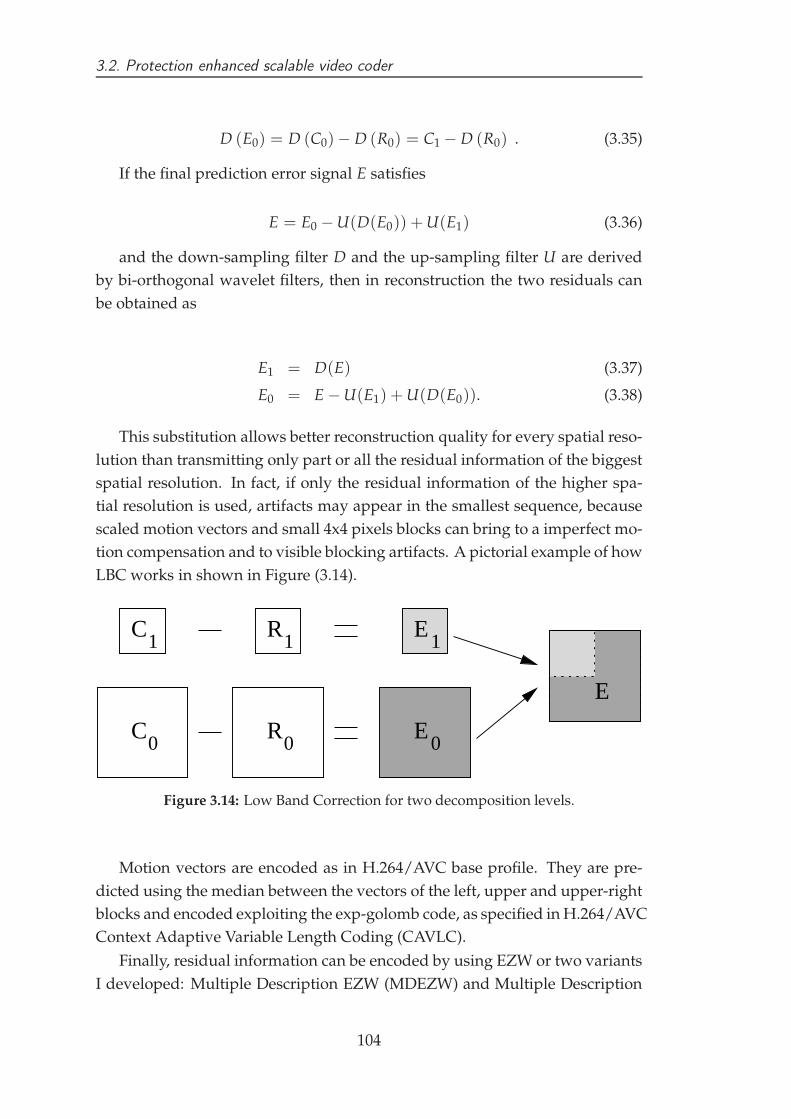
3.2. Protection enhanced scalable video coder
D (E0) = D (C0)− D (R0) = C1 − D (R0) . (3.35)
If the final prediction error signal E satisfies
E = E0 − U(D(E0)) + U(E1) (3.36)
and the down-sampling filter D and the up-sampling filter U are derived
by bi-orthogonal wavelet filters, then in reconstruction the two residuals can
be obtained as
E1 = D(E) (3.37)
E0 = E − U(E1) + U(D(E0)). (3.38)
This substitution allows better reconstruction quality for every spatial reso-
lution than transmitting only part or all the residual information of the biggest
spatial resolution. In fact, if only the residual information of the higher spa-
tial resolution is used, artifacts may appear in the smallest sequence, because
scaled motion vectors and small 4x4 pixels blocks can bring to a imperfect mo-
tion compensation and to visible blocking artifacts. A pictorial example of how
LBC works in shown in Figure (3.14).
C1
C0
R0
R1
E0
E1
E
Figure 3.14: Low Band Correction for two decomposition levels.
Motion vectors are encoded as in H.264/AVC base profile. They are pre-
dicted using the median between the vectors of the left, upper and upper-right
blocks and encoded exploiting the exp-golomb code, as specified in H.264/AVC
Context Adaptive Variable Length Coding (CAVLC).
Finally, residual information can be encoded by using EZW or two variants
I developed: Multiple Description EZW (MDEZW) and Multiple Description
104

3.2. Protection enhanced scalable video coder
Scalar Quantizer (MDSQ) based EZW. By adopting MDEZW spatial correla-
tion is exploited to generate descriptions, dividing the bands imposed by the
Discrete Wavelet Transform (DWT). In MDSQ-based EZW the residual infor-
mation is quantized by a MDSQ and the two obtained descriptions are inde-
pendently encoded by EZW. Although I never used two different MDC tech-
niques at the same time, it should not be difficult to output four descriptions
instead of two.
3.2.1 Spatial Multiple Description Coding
By excluding the MDSTAR algorithm and enabling the MDEZW [CN07] block,
spatial MDC is enabled in the encoder.
Low resolution coefficients Intermediate resolution coefficients
High resolution coefficients
Figure 3.15: Multiple descriptions construction. Low-, intermediate- and
high-resolution DWT-transformed coefficients are merged to-
gether as described in the LBC algorithm. Bands of the same
color belong to the same description. The white low band is
shared between all descriptions.
Spatial multiple descriptions are generated by splitting the output of the
LBC block during EZW coding. Particularly, each decomposition layer is di-
vided into three description exploiting the LH, HL and HH bands obtained
from the wavelet transform. During tests, it was noticed how performance in-
creased by not assigning the same subbands to the same description. In fact,
by putting an LH, an HL and a HH band in each description the reconstruc-
tion quality increases. This came at a too high price in terms of introduced re-
dundancy because it broke the structure of the zero-trees and therefore it was
105

3.2. Protection enhanced scalable video coder
decided not to take advantage of this gain of half dB in PSNR. Motion vectors
are duplicated on each description, because since they are encoded taking ad-
vantage of prediction, in case of transmission error, not only those relative to
the lost description but all motion vectors are influenced by the wrong recon-
struction. This can cause annoying artifacts, especially in this scheme, where
the same motion vector field is shared between the available resolution: in the
high resolution sequence motion vectors are doubled and therefore errors are
much more visible. Although this choice requires more bandwidth, part of this
requirement can be reduced thanks to motion vectors prediction and for high
quality videos does not excessively increase redundancy, since most bits are
used to encode the residual information. Figure (3.15) shows how coefficients
from the three resolution images are merged together using LBC and descrip-
tions are generated. Please note that in Figure (3.15) the vertical dimension
is used only to ease bands grouping and does not correspond to any imple-
mented functionality.
Since we require to be able to dynamically switch between the single de-
scription and multiple description approach, EZW coding has to be slightly
modified. Instead of iteratively scanning the bands of each decomposition
level, our implementation of EZW scans all the bands of each description. This
gives the possibility of switching between one and three descriptions and in
order to switch between resolution band scanning can be interrupted at the
desired decomposition level.
I also tried to make the introduced redundancy tunable. I tried to insert
some parity subbands to generate a fourth description used for parity check-
ing, but it turned out that these additional bands cannot be efficiently encoded
with EZW because their coefficients do not share the same inter- and intra-
band correlation. If redundancy tunability is needed, a better solution is given
by copying some low bands on more than one description, or studying over-
sampled wavelets.
3.2.2 MDSQ-based Multiple Description Coding
As already shown in Section (2.7.1), the Multiple Description Scalar Quantizer
(MDSQ) is an extension to the optimal Lloyd-Max scalar quantizer proposed
by Vaishampayan [Vai93b], where the encoder sends the information over two
different channels subject to a rate constraint. The receiver reconstructs the
received source samples from the currently working channels. The optimal
MDSQ minimizes the reconstructed signal distortion when both data chunks
are correctly transmitted, while in case of only one description reception, re-
106

3.2. Protection enhanced scalable video coder
construction is characterized by fixed average distortion.
Since it is not always possible to change the cells of the quantizer, many
MDC schemes relying on the MDSQ optimize only the reconstruction level,
thus obtaining a suboptimal system. This problem is even more important
in this coding scheme, because it works in fixed point and truncation errors
would increase computational noise. Moreover, since the optimal MDSQ re-
quires Voronoi cells whose boundaries are not bit-aligned as the cells imposed
by the bitplane encoding algorithms, it was decided only to apply the index
assignment algorithms.
Simulation results were disappointing. In fact, if the number of diagonals is
big, than the side decoders cells size is such that reconstruction quality in case
of transmission error is too low to be acceptable. Cells are so big that quanti-
zation is too aggressive and noise destroys the visual information. Following
a paper of Sun and Dai [SD], we tried to reduce the number of diagonals to
reduce cells size and therefore quantization noise. By reducing the number of
diagonal in the assignment matrix we got good reconstruction quality but the
introduced redundancy raised quickly. In fact, by using less diagonal in the
assignment matrix the output signals become more correlated, and in the case
proposed by Sun and Dai the precision of the obtained descriptions has only
one bit less then the original one and therefore the required bitrate corresponds
to encoding the image twice, skipping only the less significant bitplane.
Figure 3.16: Assignment matrix proposed by Sun and Dai. By using only two
diagonals, the first seven bits are in practice replicated.
For this reasons, after having run some tests to measure the introduced re-
dundancy, it was decided to focus on other MDC schemes and consider MDSQ
not a valid solution for SVC schemes.
107
3.2. Protection enhanced scalable video coder
3.2.3 Temporal Multiple Description Coding
By connecting the Multiple Description Successive Temporal Approximation
and Referencing (MDSTAR) block [CN], temporal MDC can be enabled in the
proposed encoder.
In MDSTAR, frames are first partitioned into even and odd. Successively,
the obtained sequences are independently encoded with the Successive Tem-
poral Approximation and Referencing (STAR) [Han03] algorithm. In STAR,
temporal scalability is obtained by doubling the number of frames in each
temporal level by dyadically decomposing them. Frames are selected by sub-
sequently visiting the levels of the binary tree obtained by the decomposition.
Depending on the availability of the reference frames, the current frame can
be encoded either as P or B. When the STAR algorithm is applied to the split
frames independently, it is possible to identify couples of frames, one in each
description, which are adjacent in the original sequence. Since these frames are
highly correlated, for each frame it is possible to store the motion vector field
obtained by the motion estimation performed by using the other frame as ref-
erence. Whenever a transmission error occurs, the lost frame can be estimated
by applying the motion vector field to the relative frame in the other descrip-
tion. An example of how MDSTAR works is given in Figure (3.17), where the
sequence dyadic decomposition is shown. The two descriptions hold either the
frames filled with a pattern or with a color and one of the two I initial frames.
The partitioning process has a major drawback in case of many temporal
decomposition levels: if the decomposition levels are more than three, then
frames in the low framerate layer are badly spaced, and the reconstructed se-
quence consists of very far couples of near frames. In this case it is not possible
to produce a smooth enough playback of the sequence. As a solution for this
specific case, the Multiple Description version of STAR has to be modified so
that the roots of the trees imposed by the dyadic decomposition are not located
in adjacent frames but they have a distance of
2l−1
2± 1
frames, where l is the number of decomposition levels. In fact, when in each
description are obtained l decomposition levels then each binary tree holds
l−1
∑n=0
2n
frames and the distance in terms of frames between the root of the tree and
the successive decomposition level frames is equal to 2l−1. As a consequence
108

3.2. Protection enhanced scalable video coder
Figure 3.17: Example of Multiple Description STAR algorithm application for
three temporal decomposition levels and 16 frames GOP. The star
algorithm is independently applied to even and off frames. Re-
dundancy is introduced by evaluating the additional motion vec-
tor fields and optionally encoding some bitplanes of the residual
information of neighbor frames.
offsetting the trees roots of 2l−1
2 ± 1 frames, the frames of a decomposition
level will be close to those of the successive decomposition layer in the other
description and therefore the maximum spread between the frames will be
achieved, because of the dyadic decomposition. The ±1 term takes into ac-
count the fact that the frames indexes must be integer.
Redundancy tunability can be introduced by varying the search range in
motion estimation between frames couples and by encoding some bitplanes of
the difference signal. However, by adjusting these parameters quality does not
significantly increases. In fact, if the input sequence has a limited motion vec-
tor field, quality does not change by increasing the search range upon a critical
range. If motion estimation is accurate, then introducing more redundancy by
encoding some bitplanes of the residual information might not be justified by
quality, especially in case of few transmission errors.
An upper bound to the introduced redundancy for each frame can be esti-
mated as
mr · mc · vm · 2 · l(r) (3.39)
bits, where mr and mc are the number of macroblocks per row, vm the num-
ber of vectors per macroblock and per column and l(r) is the maximum length
109

3.2. Protection enhanced scalable video coder
Figure 3.18: Example of Multiple Description STAR algorithm application for
four temporal decomposition levels with equally spaced frames.
in bits necessary to encode one motion vector component by using the CAVLC
syntax to encode se syntax elements. l(r) is 3 for a search range of one pixel, 5
for a three pixel search range, 7 for a seven pixel search range and so on, as it
can be easily seen in the CAVLC specification.
This estimate does not take into account the fact that by splitting even and
odd frames motion compensation loses efficiency because reference frames are
far from the encoded one. This is not considered an error, because the STAR
algorithm separates the input frames by applying a dyadic decomposition and
therefore the temporal distance does not really change and the motion com-
pensation efficiency does not change.
3.2.4 Experimental Results
In the previous chapter we adopted as test scenario the loss of a single frame in
one description to test the PSNR behavior. This scenario was realistic only in
case of low-bitrate transmissions, but by applying MDC to SVC this scenario
became inappropriate, thus, we decided to applied the so called Error Patterns
for Internet Experiments.
Since performance of the MDSQ-based approach was poor, only spatial and
temporal multiple description coding were investigated.
110

3.2. Protection enhanced scalable video coder
Test conditions
Error Patterns for Internet Experiments [Wen99], are provided to test the
schemes in case of unreliable transmission, in case of 3%, 5%, 10% and 20%
packet error rate. They have been obtained performing some experiments on
the Internet backbone to provide up-to-date information about the packet loss
characteristics. The conclusions drawn out of those experiments can be sum-
marized as follows:
• There are virtually no bit errors in IP/UDP packets;
• No relationship can be observed between the packet size and the packet
loss rate;
• No relationship can be observed between the bitrate and the packet loss
rate;
• Packet losses typically occur randomly or in very short bursts like two or
three packets;
• Packet loss rates are dependent on the connection;
• Packet loss rates are dependent on the time of day.
These patterns consist of 10000 characters with a value larger than ’0’, plus
whitespace characters. When interpreting the patterns, any whitespace char-
acters should be ignored. Each non-whitespace character reflects the delay
category of a single packet. The delay can be calculated by subtracting the
ASCII-value of ’0’ from the character reflecting the delay of a packet. The re-
sulting number should be multiplied by 10 to reflect the delay in milliseconds.
A value of ’1’, for example reflects between 0 and 10 ms delay, a value of ’5’
reflects 41-50 ms delay.
File Pattern Average Delay Loss Loss150 Loss200
3 ubc35 125 ms 3.3% 3.8% 3.4%
5 ucla194 141 ms 5.6% 5.7% 5.7%
10 ubc12 160 ms 11.5% 19.7% 13.2%
20 ubc92 160 ms 20.8% 30.0% 22.7%
Table 3.1: Statistical information for Error Patterns for Internet Experiments
In Table (3.2.4) the statistical information about the four proposed patterns
is shown, where Loss is the packet loss rate (all packets marked as ’0’ in the
111
3.2. Protection enhanced scalable video coder
error patter file), Loss150 is the packet loss rate when assuming all packets
are lost that arrive later than 150% of the average delay and Loss200 is similar
to Loss150, but assuming 200% of average delay. Loss150 and Loss200 can
be optionally used for a (very much) simplified simulation of the RTP buffer
management.
During the evaluation of these new test conditions, extremely long packet
loss bursts of more than 100 packets were rarely observed. Error patterns con-
taining such extremely long network stalls were not used for any assessment
beyond the packet loss probability calculation, as they render multimedia com-
munication useless. The most likely reaction of a user in such cases would be
to ’hang up, and dial again’. It is unclear, whether these results represent back-
bone behavior, or whether they were caused by some form of extremely high
local network utilization, e.g. due to batch backup runs or automatic software
updates in the involved LANs, but they show how the assumption in [PA97]
and [Per99] of error bursts corrupting the transmission are not verified.
3.2.5 Spatial Multiple Description Coding
Since MDEZW generates three descriptions by truncating the scanning process
of each bitplane, it is able to efficiently protect the bitstream without introduc-
ing noticeable redundancy. In fact, by not only setting to zero the coefficients
relative to other descriptions but also by truncating the scanning process, it is
able to generate the description for the residual information without duplicat-
ing any information but the motion vector field. This substantially does not
require many bits since it is differentially encoded as in H.264/AVC, and the
LL wavelet band in the smallest decomposition level. Since the number of de-
composition layers can be much higher than the number of spatial resolution,
the LL band only has a few pixels.
In Figures (3.19, 3.20) the Redundancy Rate-Distortion (RRD) region for
4CIF sequences is represented, showing the achievable PSNR by introducing
some redundancy. Results are the same for all the tested sequences, such as
“crew” or “soccer”. In these two figures, the RRD region was evaluated under
the 5% and 20% packet loss scenario respectively using 6 decomposition levels
in MDEZW.
In case smaller sequences are used, worse results can be achieved. In fact,
each time a decomposition level is added redundancy is approximately re-
duced of up to 75%. This happens because by adding an adjunctive level,
the shared LL band is further split and only one quarter of its coefficients are
shared between the descriptions. Clearly, in order to obtained the same redun-
112

3.2. Protection enhanced scalable video coder
1 1.2 1.4 1.6 1.8 2 2.2 2.4 2.6 2.8 3
18
20
22
24
26
28
30
32
34
RRD region for the multiple description encoder in case of 5% loss
Redundancy (%)
PS
NR
(dB
)
Figure 3.19: Redundancy Rate-Distortion regions for the multiple description
encoder in case of 5% packet loss probability for 4CIF sequences
sequence using 6 decomposition levels in MDEZW. Since redun-
dancy is not a degree of freedom in this scheme, each point is a
complete RRD region for a given number of bitplanes encoded.
Drawn lines show the PSNR and redundancy vary by changing
the number of encoded bitplanes.
1 1.2 1.4 1.6 1.8 2 2.2 2.4 2.6 2.8 314
16
18
20
22
24
26
28
RRD region for the multiple description encoder in case of 20% loss
Redundancy (%)
PS
NR
(dB
)
Figure 3.20: Redundancy Rate-Distortion regions for the multiple description
encoder in case of 20% packet loss probability.
113

3.2. Protection enhanced scalable video coder
dancy additional decomposition levels have to be added and in case of infor-
mation loss less data is available for reconstruction, leading to worse quality.
Thus, the number of decomposition levels is a trade-off, because the less coef-
ficients are shared the more fragile the coding scheme becomes.
0 5 10 15 20 25 3020
25
30
35
40
45
Transmission simulation of CIF sequence foreman
Frame number
PS
NR
(dB
)
0% packet loss3% packet loss with MDC5% packet loss with MDC3% packet loss without MDC5% packet loss without MDC
Figure 3.21: Comparison of the decoded sequence quality for 0%, 3% and 5%
packet loss probability using SVC and MDC schemes and the
“foreman” CIF sequence.
It is important to notice that this coding scheme does not allow the user
to choose the amount of redundancy introduced, and therefore RRD region
consists of only one point. The drawn lines in these figures show how the
introduced redundancy and the PSNR of the reconstructed sequence change
by varying the number of encoded bitplanes. The more bitplanes yield higher
quality of the reconstructed sequence and at the same time fewer redundancy
because it consists only of the motion vector field.
The quality of the decoded sequence was compared at the receiver in the
single and multiple description cases, assuming that in case of packet loss in
the single description decoder the frame is discarded. For the single descrip-
tion encoder each packet consists of one frame, while for the single encoder,
114

3.2. Protection enhanced scalable video coder
0 5 10 15 20 25 30
20
25
30
35
40
45
Transmission simulation of CIF sequence foreman
Frame number
PS
NR
(dB
)
0% packet loss10% packet loss with MDC20% packet loss with MDC10% packet loss without MDC20% packet loss without MDC
Figure 3.22: Comparison of the decoded sequence quality for 0%, 10% and
20% packet loss probability using SVC and MDC schemes and
the “foreman” CIF sequence.
115

3.2. Protection enhanced scalable video coder
each packet hold one frame description. Since single description packets are
approximately as big as three multiple description packets, the probability of
packet loss in case of SVC is three times the probability of loosing one packet
during MDC. In Figures (3.21, 3.22) the comparison results of SVC and MDC
are shown for the proposed packet loss patterns using the “foreman” CIF se-
quence coding seven bitplanes.
An example of what the distortion looks like is shown in Figure (3.23),
where the decoded sequence “foreman” is reported after having lost five pack-
ets. Each packet loss corresponds to some coefficients of the residual signal
having value of zero, therefore the introduced artifacts are very similar to those
affecting images lossy compressed by interrupting the bitplane encoding be-
fore all the coefficients bits have been properly encoded.
Figure 3.23: Example of video corruption after five transmission errors for
MDEZW. The introduced distortion is similar to the artifacts ob-
tained in image compression by truncating the bitplane encod-
ing before all coefficients have been compressed at the resolution
necessary for lossless encoding.
Keeping in mind the small amount of introduced redundancy, it can be
concluded that the achieved result is positive. In fact, by qualitatively compar-
ing this scheme with those developed for the H.264/AVC encoder, not only
this scheme offers good protection requiring only very small redundancy, but
116

3.2. Protection enhanced scalable video coder
at the same time it can be easily integrated into SVC schemes, because of its
simplification and minimal modification of the EZW algorithm.
3.2.6 Temporal Multiple Description Coding
0 1 2 3 4 5 6 7 8 9 10 1142
42.5
43
43.5
44
44.5
45
45.5
Redundancy %
PS
NR
(dB
)MDSTAR RRD region
3% packet loss5% packet loss10% packet loss20% packet loss
Figure 3.24: Redundancy Rate-Distortion for the “foreman” CIF sequence. The
average PSNR of the decode sequence afflicted by transmission
error is plotted against the introduced redundancy for 3%, 5%
10% and 20% error probability.
The first test for MDSTAR was the evaluation of the RRD region. The
amount of redundancy cannot be easily tuned, as it can appear. In fact, what
makes Equation (3.39) an upper bound is the fact that motion vectors are pre-
dictively encoded and therefore increasing r does not always increase the bits
necessary to hold l(r). If the input sequence has an uniform motion vector
field the introduced redundancy is significantly smaller and does not change
by varying r. Since redundancy consists of only a few bits if compared to the
total bitstream, redundancy can be further and better tuned by storing not only
the motion vector field between the couples of frames, but also some bitplanes
of the residual information from motion estimation.
As tests have shown, the RRD region is in practice flat, and it only varies
of portions of dB when adding several bitplanes in the information that links
frames in each couple. Obviously, the reconstruction quality is dependent from
117

3.2. Protection enhanced scalable video coder
the percentage of lost packets, so in Figure (3.24) the four regions correspond-
ing to the four Error Patterns are shown. The flatness of such regions led to the
choice of not including any additional bitplanes in the successive tests.
0 5 10 15 20 25 3030
32
34
36
38
40
42
44
46
48Transmission simulation of CIF sequence foreman
Frame number
PS
NR
(dB
)
0% packet loss3% packet loss with MDC5% packet loss with MDC
Figure 3.25: Transmission simulation if the “foreman” CIF sequence com-
pressed with the MDSTAR algorithm. In this case the 3% and
5% error patterns are used.
Figures (3.25, 3.26) show how the PSNR of the “foreman” sequence at CIF
resolution varies in case of errors. In Figure (3.25) the 3% and 5% error patterns
are used, while in Figure (3.26) 10% and 20% packet loss probabilities are used.
All tests evince that PSNR losses are not homogeneous, but significantly varies
from frame to frame. The flickering quality is due to the even and odd frames
separation and dyadic decompositions.
In fact, even and odd separation is the main reason for alternating quality
frames, but the dyadic decomposition explains why errors afflict only a few
frames and do not span the successive frames. In the hierarchic decomposition,
most errors corrupt frames in the binary tree of the affected frame. Moreover,
since in the dyadic decomposition B frames are massively used, if the currently
decoded frame has one corrupted reference, the unaffected one smoothes the
118

3.2. Protection enhanced scalable video coder
reconstruction errors because they are averaged for prediction.
0 5 10 15 20 25 3030
32
34
36
38
40
42
44
46
48Transmission simulation of CIF sequence foreman
Frame number
PS
NR
(dB
)
0% packet loss10% packet loss with MDC20% packet loss with MDC
Figure 3.26: Transmission simulation if the “foreman” CIF sequence com-
pressed with the MDSTAR algorithm. In this case the 10% and
20% error patterns are used.
The only case when errors propagate on successive decomposition tree
happens when the root of the tree is corrupted. In fact, the tree root is used
to predict as P the next tree root, thus errors can propagate. To contrast this,
two solutions are available:
• increasing the number of decomposition levels. Each time a temporal
decomposition level is added, the number of roots is halved, as the prob-
ability of corruption of such frames is reduced. This strategy does not
directly stop distortion propagation, but the levels number can be jointly
chosen with the GOP size, so that the maximum tolerable distortion can
be obtained.
• save additional residual bitplanes only for trees roots. This prevents
error propagation. If all the residual information is encoded errors are
stopped, but usually not all the bitplanes are necessary, especially when
119

3.2. Protection enhanced scalable video coder
prediction is efficient. Moreover, if a tree root is corrupted and errors cor-
rupt its reconstruction, even the successive root can be reconstructed by
motion-compensating the correctly received roots in the other descrip-
tions.
Figure (3.27) is a final example, where the eleventh, thirteenth and fifteenth
frames of the “foreman” sequence are respectively shown in 3.27(a), 3.27(b)
and 3.27(c). The sequence transmission is flawless, wit the exception of the
thirteenth frame, which is lost. Since the error originates in the thirteenth
frame and redundancy consists only of the motion vector field, in 3.27(b) the
blocking artifacts due to the mere motion compensation can be seen. The
eleventh frame is encoded as B from the ninth and thirteenth frames and there-
fore in 3.27(a) distortion is reduced by bidirectional motion compensation. The
fifteenth frame in 3.27(c) is encoded as P frame using the thirteenth frame as
reference and decoder drift increases because of the bad-quality reference.
3.2.7 Comparison between the spatial and temporal approaches
MDEZW and MDSTAR have opposite characteristics that make them hard to
use together, as it was hoped at the beginning of the Protection Enhanced Scal-
able Video Encoder.
The spatial approach is extremely light in terms of computational overhead,
because no additional operation is required if compared to the single descrip-
tion encoder. Further more, prediction is not altered by switching from the sin-
gle description to the multiple description encoder, so the bitstream extractor
or an hypothetical relay server can dynamically switch from the SD to the MD
configuration and vice-versa, depending on the channels statistics. Therefore,
theoretically is possible to execute the first version on the encoder in real-time,
given an appropriate optimization of the code.
Contrarily, MDSTAR involves several additional operation of motion es-
timation and compensation. Even the coding order is different, so it is not
possible is dynamically switch from the single description to the multiple en-
coder, but the compressed bitstream have to be separately generated. This is
the reason why MDEZW and MDSTAR cannot be work together in real-time
in a scalable encoder.
By comparing the corresponding Redundancy Rate-Distortion regions, it
can be seen that in both algorithms the introduced redundancy is small, but
MDSTAR is able to better exploit it. In fact, for a comparable amount of redun-
dancy, it clearly appears that the mean output quality of MDSTAR is superior
120

3.2. Protection enhanced scalable video coder
(a)
(b)
(c)
Figure 3.27: Example of introduced distortion in case of transmission error for
MDSTAR.
121

3.2. Protection enhanced scalable video coder
to MDEZW, as the transmission simulation confirm. On the other hand, the
computational requirements of MDSTAR make it hard to adopt it, because of
all the necessary motion compensation operation at the decoder, which can be
a mobile device with reduced computational resources, and also because the
dyadic decomposition introduces a significant decode delay that requires to
store in the frame buffer many more frames then MDEZW. The latter, event
tough offers less protection to errors, can be nearly implemented for free in
terms of CPU and memory. Thus, it is the candidate for future applications
to scalable video coding for future distributed applications, such P2P video
streaming.
As final remark, qualities of MDEZW and MDSTAR are summarized in
Table (3.2.7).
MDEZW MDSTAR
Exploited correlation spatial temporal
Efficiency good good
Computational Cost low high
Tunability no yes
Switchable between SDC and MDC yes no
Table 3.2: Qualitative comparison of MDZW and MDSTAR.
122

Chapter 4
Conclusions
The topic of this thesis is reliable transmission of non-scalable and scalable
video. Among several different strategies, Multiple Description Coding is a
joint source channel technique which aims to add robustness by dividing the
input signal in subsampled portions and by sending them over distinct chan-
nels, in order to exploit the channel diversity. One main characteristic of Mul-
tiple Description Coding is the fact that joint source channel coding is mainly
focused on source coding and possible signal division strategies are chosen
starting from the coding scheme and not from the channel statistics, as other
joint source channel solutions do.
With the exception of implementing it as pre- and post-processing opera-
tions, application of Multiple Description Coding is in general hard, especially
when these techniques are added to an already existing coding standard.
This is the case of H.264/AVC, where schemes based on spatial or tempo-
ral input subsampling can be easily implemented but can lead to misfunction.
In fact, spatial subsampling breaks Intra prediction, while temporal subsam-
pling reduces motion compensation efficiency because it forces motion esti-
mation on temporally far frames. Other schemes cannot be implemented as
pre- and post-processing blocks, so they require heavy changes in the encoder
source code. Even the solution based on a Multiple Description Scalar Quan-
tizer, which eventually was implemented as a lookup table, required a deep
study of the code before being able to implement it. The worst case was the
Motion-Compensated Multiple Description Video coding, which required sev-
eral thousands of lines of code to fit the JVT reference encoder.
In the scalable video case, application of MDC was easier, because some
coding strategies were decided by keeping into account the encoder design
and the generated descriptions. As an example, the Le Gall 5/3 wavelet was
chosen because it is the optimal trade-off between computational complexity
123
and output quality of the Single Description and Multiple Description cases.
Wavelets with longer filters were under examination, because by increasing the
filter size the correlation of the wavelet coefficients rises, thus making possible
to introduce an estimation of lost coefficients. The major drawback of this
approach was the reduction of the compression ratio and of the output quality
of the single description decoder, because long filters tend to degrade edges
sharpness in the frames, so eventually it was chosen not to pursue this strategy.
Only by adding support to Multiple Description Coding during standards
definition, as it happened for other tools such as Data Partitioning and Flexible
Macroblock Ordering in the H.264/AVC standard, it will be possible to apply
these techniques. Fortunately, emerging scenarios in Scalable Video Coding
and Peer-to-Peer video streaming over non-homogeneous networks seem to
be the suitable environment where these techniques will be fully exploited.
Future steps in Multiple Description Coding research applied to Scalable
Video Coding will aim to increase compression efficiency and redundancy tun-
ability. The first goal will be addressed by enhancing motion compensation
and by substituting EZW with arithmetic encoding. Hopefully, better man-
agement of the introduced redundancy in spatial MDC will be obtained by
adopting new overcomplete wavelet transforms, whose additional bands will
be used as parity check bands that can be efficiently compressed. Finally, di-
rectional wavelets can be further investigated to rise compression ratios.
124

Bibliography
[Ahl85] R. Ahlswede. The rate-distortion region for multiple descrip-
tions without excess rate. IEEE Transactions on Information Theory,
31(6):721–726, 1985.
[AK00] M.D. Adams and F. Kossentini. Reversible Integer-to-Integer
Wavelet Transforms for Image Compression: Performance Evalua-
tion and Analysis. IEEE TRANSACTIONS ON IMAGE PROCESS-
ING, 9(6), 2000.
[Apo00] J. Apostolopoulos. Error resilient video compression through the
use of multiple states,. Proc. IEEE Int. Conf. Image Processing, 3:352–
355, 2000.
[Apo01a] J. Apostolopoulos. Reliable video communication over lossy
packet networks using Multiple State Encoding and path diver-
sity. In IEEE VCIP 2001, January 2001.
[Apo01b] J. Apostolopoulos. Unbalanced Multiple Description video com-
munication using path diversity. In Proc. of International Conference
on Image Processing, ICIP 2001, Thessaloniki, Greece, October 2001.
[AW01] MD Adams and R. Ward. Wavelet transforms in the JPEG-2000
standard. Communications, Computers and signal Processing, 2001.
PACRIM. 2001 IEEE Pacific Rim Conference on, 1, 2001.
[BRTV04] R. Bernardini, R. Rinaldo, A. Tonello, and A. Vitali. Frame based
multiple description for multimedia transmission over wireless
networks. In Proc. of 7th Int. Symp. WPMC, volume 2, pages 529–
532, Abano Terme, Italy, July 2004.
[CCD+06] O. Campana, A. Cattani, A. De Giusti, S. Milani, N. Zandonà,
and G. Calvagno. Multiple Description Coding Schemes for the
125

BIBLIOGRAPHY
H.264/AVC Coder. In Proc. of the International Conference on Wire-
less Reconfigurable Terminals and Platforms (WiRTeP), pages 217–221,
Rome, Italy, April 2006.
[CDSY98] AR Calderbank, I. Daubechies, W. Sweldens, and B.L. Yeo.
Wavelet transforms that map integers to integers. Appl. Comput.
Harmon. Anal, 5(3):332–369, 1998.
[CM04] O. Campana and S. Milani. A Multiple Description Coding
Scheme For The H.264/AVC Coder. In Proc. of the International
Conference on Telecommunication and Computer Networks IADAT-
tcn2004, pages 191–195, San Sebastian, Spain, December 2004.
[CN] O. Campana and T. Nguyen. A Temporal Multiple Description
Coding Based Scalable Video Codec.
[CN07] O. Campana and T. Nguyen. Protection Enhanced Scalable Video
Coding. In Proc. of the 15th European Signal Processing Conference
(EUSIPCO 2007), Poznan, Poland, September 2007.
[CT06] T. M. Cover and J. A. Thomas. Elements of Information Theory.
Wiley-Interscience New York, 2006.
[DIS91] ISO DIS. 10918-1. Digital Compression and Coding of Continuous-tone
Still Images (JPEG), CCITT Recommendation T, 81, 1991.
[DMW03] H. Schwarz D. Marpe and T. Wiegand. Context-based adaptive bi-
nary arithmetic coding in the H.264/AVC video compression stan-
dard. IEEE Transactions on Circuits and Systems for Video Technology,
13(7):620–636, 2003.
[DS98] I. Daubechies and W. Sweldens. Factoring wavelet transforms into
lifting steps. Journal of Fourier Analysis and Applications, 4(3):247–
269, 1998.
[EF95] S. Eckart and C. Fogg. ISO/IEC MPEG-2 software video codec.
Proc. SPIE, 2419:100–118, 1995.
[GC82] Abbas A. El Gamal and Thomas M. Cover. Achievable rates for
multiple descriptions. IEEE Transactions on Information Theory, IT-
28(6):851–857, November 1982.
[Ger79] A. Gersho. The channel splitting problem and modulo-PCM cod-
ing. Bell Labs Memo for Record (not archived), October 1979.
126

BIBLIOGRAPHY
[GK98] V.K. Goyal and J. Kovacevic. Optimal multiple description trans-
form coding of Gaussian vectors. Proc. IEEE Data Compression Conf,
pages 388–397, 1998.
[GKAV98] VK Goyal, J. Kovacevic, R. Arean, and M. Vetterli. Multiple de-
scription transform coding of images. Image Processing, 1998. ICIP
98. Proceedings. 1998 International Conference on, 1, 1998.
[Goy01a] Vivek K. Goyal. Multiple description coding: Compression meets
the network. IEEE Signal Processing Magazine, 8(5):74–93, Septem-
ber 2001.
[Goy01b] Vivek K. Goyal. Single and Multiple Description Transform Cod-
ing with Bases and Frames. In Proc. of SIAM, 2001.
[Gra95] A. Graps. An introduction to wavelets. IEEE Computational Science
and Engineering, 2(2):50–61, 1995.
[GVT98] VK Goyal, M. Vetterli, and NT Thao. Quantized overcomplete ex-
pansions in IR N: analysis, synthesis, and algorithms. IEEE Trans-
actions on Information Theory, 44(1):16–31, 1998.
[Han03] W. J. Han. Successive Temporal Approximation and Referencing
(STAR) for Improving MCTF in Low End-to-end Delay Scalable
Video Coding. ISO/IEC JTC 1/SC 29/WG11 M10308, December
2003.
[Han04] W. J. Han. Responses of call for proposal for scalable video coding.
ISO/IEC JTC 1/SC 29/WG11 MPEG2004/M10569/ S, March 2004.
[HPCH07] H.C. Huang, W.H. Peng, T. Chiang, and H.M. Hang. Advances
in the scalable amendment of H.264/AVC. IEEE Communications
Magazine, 45(1):68–76, 2007.
[Jay81] N.S. Jayant. Sub-sampling of a DPCM speech channel to provide
two “self-contained” half-rate channels. Bell Syst. Tech J., 60(4):501–
509, April 1981.
[Kai74] JF Kaiser. Nonrecursive digital filter design using the I 0-sinh win-
dow function. Proc. IEEE Int. Symp. Circuits Syst, 3:20–23, 1974.
[KL01] C. Kim and S. Lee. Multiple description coding of motion fields
for robust video transmission. IEEE Transactions on Circuits and
Systems for Video Technology, 11(9):999–1010, September 2001.
127

BIBLIOGRAPHY
[KXP97] B.J. Kim, Z. Xiong, and W.A. Pearlman. Very low bit-rate embed-
ded video coding with 3D set partitioning in hierarchical trees (3D
SPIHT). IEEE Transactions on Circuits and Systems for Video Technol-
ogy, 1997.
[Li01] W. Li. Overview of fine granularity scalability in MPEG-4 video
standard. Circuits and Systems for Video Technology, IEEE Transac-
tions on, 11(3):301–317, 2001.
[LJL+03] P. List, A. Joch, J. Lainema, G. Bjntegaard, and M. Karczewicz.
Adaptive deblocking filter. IEEE Transactions on Circuits and Sys-
tems for Video Technology, 13(7):614–619, 2003.
[Mal89] SG Mallat. A theory for multiresolution signal decomposition: the
waveletrepresentation. Pattern Analysis and Machine Intelligence,
IEEE Transactions on, 11(7):674–693, 1989.
[MCO] C. Mayer, H. Crysandt, and J.R. Ohm. Bit plane quantization for
scalable video coding. Proc. SPIE Visual Communications and Image
Processing02, pages 1142–1152.
[Mil80] Stewart E. Miller. Fail-safe transmission without standby facilities.
Technical report, Bell Labs, Tech. Rep. TM80-136-2, August 1980.
[Mil83] Stewart E. Miller. Fail-safe transmission system, January 1983.
[MWG05] D. Marpe, T. Wiegand, and S. Gordon. H.264/MPEG4-AVC Fi-
delity Range Extensions: Tools, Profiles, Performance and Appli-
cation Areas. Image Processing, 2005. ICIP 2005. IEEE International
Conference on, 1, 2005.
[Ohm91] JR Ohm. A hybrid image coding scheme for ATM networks based
on SBC-VQ and tree encoding. Proceedings of the Fourth Interna-
tional WorkshopPacket Video, Kyoto, August, pages 2–1, 1991.
[Ohm94] J.R. Ohm. Three-dimensional subband coding with motion com-
pensation. IEEE Transactions on Image Processing, 3(5):559–571,
1994.
[Ohm05] J.R. Ohm. Advances in Scalable Video Coding. Proceedings of the
IEEE, 93(1):42–56, 2005.
128
BIBLIOGRAPHY
[oII96] Joint Video Team (JVT) of ISO/IEC MPEG and ITU-T SG 15. Draft
recommendation h.263 “video coding for low bitrate communica-
tion”. In Joint Video Team (JVT) of ISO/IEC MPEG & ITU-T VCEG
(ISO/IEC JTC1/SC29/WG11 and ITU-T SG16 Q.6), June 1996.
[OS75] AV Oppenheim and RW Schafer. Digital signal processing. Re-
search supported by the Massachusetts Institute of Technology, Bell Tele-
phone Laboratories, and Guggenheim Foundation. Englewood Cliffs, NJ,
Prentice-Hall, Inc., 1975. 598 p., 1975.
[OWVR97] M.T. Orchard, Y. Wang, V. Vaishampayan, and A.R. Reibman. Re-
dundancy rate-distortion analysis of multiple description coding
using pairwise correlating transforms. Proc. IEEE Int. Conf. Image
Processing, 1:608–611, 1997.
[Oza80] L. Ozarow. Source-Coding Problem with Two Channels and Three
Receivers. BELL SYS. TECH. J., 59(10):1909–1921, 1980.
[PA97] Fernando Pereira and Thierry Alpert. MPEG-4 video subjective
test procedures and results. IEEE Transactions on Circuits and Sys-
tems for Video Technology, 7(1):32–51, 1997.
[Per99] F. Pereira. MPEG-4 testing and evaluation procedures document,
DOC. ISO. Technical report, IEC JTC1/SC29/WG11, 1999.
[PPB01] B. Pesquet-Popescu and V. Bottreau. Three-dimensional lifting
schemes for motion compensated videocompression. Acoustics,
Speech, and Signal Processing, 2001. Proceedings.(ICASSP’01). 2001
IEEE International Conference on, 3, 2001.
[Rec90] H. Recommendation. 261: Video codec for audiovisual services at
p x 64 kb/s. CCITT White Book, 1990.
[Ric03] Ian E. G. Richardson. H.264 and MPEG-4 video compression: video
coding for the next-generation multimedia. Wiley, Chichester, 2003.
[RJW+02] Amy R. Reibman, Hamid Jafarkhani, Yao Wang, Michel T. Or-
chard, and Rohit Puri. Multiple-description video coding us-
ing motion-compensated temporalprediction. IEEE Transactions on
Circuits and Systems for Video Technology, 12(3):193–204, 2002.
[RMR+04] R. Bernardini, M. Durigon, R. Rinaldo, L. Celetto, and A. Vi-
tali. Polyphase spatial subsampling multiple description coding of
129
BIBLIOGRAPHY
video streams with H264. In Proceedings of ICIP, volume 5, pages
3213–3216, Singapore, October 2004.
[RWS05] J. Reichel, M. Wien, and H. Schwarz. Joint Scalable Video Model
JSVM-3 Annex S. JVT-P202, Poznan, Poland, July, 2005.
[SA96] A. Said and W. A.Pearlman. A New, Fast, and Efficient Image
Codec Based on Set Partitioning in Hierarchical Trees. IEEE Trans-
actions on Circuits and Systems for Video Technology, 6(3):243–250,
1996.
[SCP93] J. M. Shapiro, D. S. R. Center, and N. J. Princeton. Embedded Im-
age Coding Using Zerotrees of Wavelet Coefficients. IEEE Trans-
actions on Signal Processing, 41(12):3445–3462, 1993.
[SD] Y. Sun and Q. Dai. Multiple Description Image Codec for Error
Prone Channels.
[SR] M. Standard and ISO Recommendation. IEC-11172-2 (1993). No
Author. No Place of Publication, pages 89–129.
[TM02] D. S. Taubman and M. Marcellin. Jpeg 2000: Image Compression
Fundamentals, Standards and Practice. Kluwer Academic Publishers,
2002.
[TWJ98] J. Tian and RO Wells Jr. Embedded Image Coding Using Wavelet
Difference Reduction. Wavelet Image and Video Compression, pages
289–301, 1998.
[Vai93a] PP Vaidyanathan. Multirate systems and filter banks. Prentice-Hall,
Inc. Upper Saddle River, NJ, USA, 1993.
[Vai93b] Vinay Anant Vaishampayan. Design of Multiple Description
Scalar Quantizers. IEEE Transactions on Information Theory,
39(3):821–833, May 1993.
[VK95] M. Vetterli and J. Kovacevic. Wavelets and subband coding. Prentice-
Hall, Inc. Upper Saddle River, NJ, USA, 1995.
[Wed03] T. Wedi. Motion compensation in H.264/AVC. IEEE Transactions
on Circuits and Systems for Video Technology, 13(7):577–586, 2003.
[Wen99] S. Wenger. Proposed error patterns for internet experiments. ITU-
T Study Group 16 H.263+ Video Experts Group, 15, 1999.
130

BIBLIOGRAPHY
[WOVR01] Y. Wang, MT Orchard, V. Vaishampayan, and AR Reibman. Multi-
ple description coding using pairwise correlating transforms. Im-
age Processing, IEEE Transactions on, 10(3):351–366, 2001.
[WSBL03] T. Wiegand, G.J. Sullivan, G. Bjntegaard, and A. Luthra. Overview
of the H.264/AVC video coding standard. IEEE Transactions on
Circuits and Systems for Video Technology, 13(7):560–576, 2003.
[Zam99] R. Zamir. Gaussian codes and Shannon bounds for multiple de-
scriptions. IEEE Transactions on Information Theory, 45(7):2629–
2636, 1999.
[ZB87] Zhen Zhang and Toby Berger. New Results in Binary Multiple
Descriptions. IEEE Transactions on Information Theory, 33(4):502–
521, 1987.
[ZMD05] N. Zandonà, S. Milani, and A. De Giusti. Motion-Compensated
Multiple Description Video Coding for the H.264/AVC Standard.
In Proc. of IADAT International Conference on Multimedia, Image Pro-
cessing and Computer Vision, pages 290–294, Madrid, Spain, March
2005.
131