MULTIPHYSICS MODELING OF THE STEEL CONTINUOUS CASTING PROCESS

BY

LANCE C. HIBBELER

DISSERTATION

Submitted in partial fulfillment of the requirementsfor the degree of Doctor of Philosophy in Mechanical Engineering

in the Graduate College of theUniversity of Illinois at Urbana–Champaign, 2014

Urbana, Illinois

Doctoral Committee:

Professor Brian G. Thomas, Chair and Director of ResearchProfessor Armand J. BeaudoinProfessor Jonathan A. DantzigProfessor Alan W. Cramb, Illinois Institute of Technology

Abstract

This work develops a macroscale, multiphysics model of the continuous casting of steel. Thecomplete model accounts for the turbulent flow and nonuniform distribution of superheat inthe molten steel, the elastic-viscoplastic thermal shrinkage of the solidifying shell, the heattransfer through the shell-mold interface with variable gap size, and the thermal distortion ofthe mold. These models are coupled together with carefully constructed boundary conditionswith the aid of reduced-order models into a single tool to investigate behavior in the moldregion, for practical applications such as predicting ideal tapers for a beam-blank mold.

The thermal and mechanical behaviors of the mold are explored as part of the overallmodeling effort, for funnel molds and for beam-blank molds. These models include highgeometric detail and reveal temperature variations on the mold-shell interface that maybe responsible for cracks in the shell. Specifically, the funnel mold has a column of moldbolts in the middle of the inside-curve region of the funnel that disturbs the uniformity ofthe hot face temperatures, which combined with the bending effect of the mold on the shell,can lead to longitudinal facial cracks. The shoulder region of the beam-blank mold showsa local hot spot that can be reduced with additional cooling in this region. The distortedshape of the funnel mold narrow face is validated with recent inclinometer measurementsfrom an operating caster. The calculated hot face temperatures and distorted shapes of themold are transferred into the multiphysics model of the solidifying shell.

The boundary conditions for the first iteration of the multiphysics model come fromreduced-order models of the process; one such model is derived in this work for mold heattransfer. The reduced-order model relies on the physics of the solution to the one-dimensionalheat-conduction equation to maintain the relationships between inputs and outputs of themodel. The geometric parameters in the model are calibrated such that the reduced-ordermodel temperatures match a small, periodic subdomain of the mold. These parametersare demonstrated to be insensitive to the calibration conditions. The thermal behavior ofthe detailed, three-dimensional mold models used in this work can be approximated closelywith a few arithmetic calculations after calibrating the reduced-order model of mold heattransfer.

The example application of the model includes the effects of the molten steel jet onthe solidification front and the ferrostatic pressure. The model is demonstrated to matchmeasurements of mold heat removal and the thickness of a breakout shell all the way aroundthe perimeter of the mold, and gives insight to the cause of breakouts in a beam-blank caster.This multiphysics modeling approach redefines the state of the art of process modeling forcontinuous casting, and can be used in future work to explore the formation and preventionof defects and other practical issues.

This work also explores the eigen-problem for an arbitrary 3x3 matrix. An explicit,algebraic formula for the eigenvectors is presented.

ii

to the radiant C. T.,

may you find the answers to all of your questions

iii

Acknowledgments

This work would not have been possible without the support of several people. First and

foremost, I thank my advisor, Professor Brian G. Thomas, for his enthusiastic support and

technical expertise provided to me over the last few years, and for demonstrating to me that

“research scientist” and “engineer” are not mutually exclusive professions. All of my teachers

over the years deserve acknowledgment, but Professors Armand Beaudoin and Jon Dantzig

are particularly noteworthy for their instruction in, and my subsequent fascination with,

continuum mechanics and solidification phenomena. I also thank Professor Alan Cramb

(Illinois Institute of Technology) for serving on my committee.

I gratefully acknowledge the financial support of the member companies of the Continuous

Casting Consortium at The University of Illinois, which have included abb, ArcelorMittal,

Baosteel, Delavan/Goodrich, Magnesita Refractories, Nippon Steel and Sumitomo Metal

Corporation, Nucor Steel, postech/posco, ssab, Steel Dynamics, Tata Steel, and ansys.

Equally gratefully I acknowledge the financial support provided by the Department of Me-

chanical Science and Engineering in the form teaching assistantships, the Alumni Teaching

Fellowship, the Eugene and Lina Abraham Fellowship, and the Alwin Schaller Travel Grant.

Some of the computational resources utilized for this work were provided by the National

Center for Supercomputing Applications (ncsa) at the University of Illinois, namely the

computing clusters Tungsten, Cobalt, Abe, and Blue Waters.

I would like to thank some of the other students and visiting scholars in the Depart-

ment of Mechanical Science and Engineering for their camaraderie and many shared meals

during my tenure at the University of Illinois, including: Eric Badger, James Buckland,

Rajneesh Chaudhary, Seong-Mook Cho, Prathiba Duvvuri, Eric Eckstrum, Sean Hamel,

Mark Hernquist, Inwho Hwang, Junya Iwasaki, Hemanth Jasti, Kai Jin, A. S. M. Jon-

ayat, Brendan Joyce, Sushil Kumar, Yonghui Li, Rui Liu, Russell McDonald, Joe Miksan,

Becky Mudrock, Aravind Murali, Claudio Ojeda, Mike Okelman, Bryan Petrus, Matt Rowan,

Mike Sangid, Varun Singh, Pete Srisuk, Kenny Swartz, Jason Troutner, Kun Xu, Matt Zap-

pulla, Xiaoxu Zhou, and the members of the Alpha chapter of Pi Tau Sigma.

Finally, I thank my family for their support of my endeavors in higher education.

iv

Table of Contents

List of Figures . . . . . . . . . . . . . . . . . . . . . . . . . . . . . . . . . . . . . vii

List of Tables . . . . . . . . . . . . . . . . . . . . . . . . . . . . . . . . . . . . . x

Chapter 1 Introduction . . . . . . . . . . . . . . . . . . . . . . . . . . . . . . . 1

Chapter 2 Steady-State Thermal Behavior of the Mold . . . . . . . . . . . . 52.1 Introduction . . . . . . . . . . . . . . . . . . . . . . . . . . . . . . . . . . . . 52.2 Model Description . . . . . . . . . . . . . . . . . . . . . . . . . . . . . . . . 52.3 Beam-Blank Mold . . . . . . . . . . . . . . . . . . . . . . . . . . . . . . . . . 82.4 Funnel Mold . . . . . . . . . . . . . . . . . . . . . . . . . . . . . . . . . . . . 192.5 Conclusions . . . . . . . . . . . . . . . . . . . . . . . . . . . . . . . . . . . . 25

Chapter 3 Reduced-Order Model of Mold Heat Transfer . . . . . . . . . . . 263.1 Introduction . . . . . . . . . . . . . . . . . . . . . . . . . . . . . . . . . . . . 263.2 Three-Dimensional Mold Model: Snapshot Model . . . . . . . . . . . . . . . 293.3 Reduced-Order Model of Mold Heat Transfer . . . . . . . . . . . . . . . . . . 303.4 Reduced-Order Model Parameter Calibration . . . . . . . . . . . . . . . . . . 403.5 Example Mold Geometries . . . . . . . . . . . . . . . . . . . . . . . . . . . . 443.6 Sensitivity of Mold Geometry Calibrations to Model Parameters . . . . . . . 503.7 Conclusions . . . . . . . . . . . . . . . . . . . . . . . . . . . . . . . . . . . . 51

Chapter 4 Steady-State Mechanical Behavior of the Mold . . . . . . . . . . 524.1 Introduction . . . . . . . . . . . . . . . . . . . . . . . . . . . . . . . . . . . . 524.2 Model Description . . . . . . . . . . . . . . . . . . . . . . . . . . . . . . . . 534.3 Bolt Calculations . . . . . . . . . . . . . . . . . . . . . . . . . . . . . . . . . 554.4 Beam-Blank Mold . . . . . . . . . . . . . . . . . . . . . . . . . . . . . . . . . 624.5 Funnel Mold . . . . . . . . . . . . . . . . . . . . . . . . . . . . . . . . . . . . 664.6 Online Measurement of Mold Distortion and Taper . . . . . . . . . . . . . . 844.7 Conclusions . . . . . . . . . . . . . . . . . . . . . . . . . . . . . . . . . . . . 84

Chapter 5 Multiphysics Model of Continuous Casting . . . . . . . . . . . . 895.1 Introduction . . . . . . . . . . . . . . . . . . . . . . . . . . . . . . . . . . . . 895.2 Solidifying Shell Model . . . . . . . . . . . . . . . . . . . . . . . . . . . . . . 905.3 Fluid Flow Model . . . . . . . . . . . . . . . . . . . . . . . . . . . . . . . . . 945.4 Mold Model . . . . . . . . . . . . . . . . . . . . . . . . . . . . . . . . . . . . 985.5 Fluid/Shell Interface Treatment . . . . . . . . . . . . . . . . . . . . . . . . . 985.6 Shell/Mold Interface Treatment . . . . . . . . . . . . . . . . . . . . . . . . . 1025.7 Validation of the Numerical Models . . . . . . . . . . . . . . . . . . . . . . . 104

v

5.8 Multiphysics Model of Beam-Blank Casting . . . . . . . . . . . . . . . . . . 1075.9 Conclusions . . . . . . . . . . . . . . . . . . . . . . . . . . . . . . . . . . . . 113

Chapter 6 Conclusions and Future Work . . . . . . . . . . . . . . . . . . . . 116

Appendix A Mold Geometry . . . . . . . . . . . . . . . . . . . . . . . . . . . . 119A.1 Funnel Mold . . . . . . . . . . . . . . . . . . . . . . . . . . . . . . . . . . . . 119A.2 Beam-Blank Mold . . . . . . . . . . . . . . . . . . . . . . . . . . . . . . . . . 124

Appendix B The Eigenvalues and Eigenvectors of a 3× 3 Matrix . . . . . . 127B.1 Introduction . . . . . . . . . . . . . . . . . . . . . . . . . . . . . . . . . . . . 127B.2 Calculating the Eigenvalues . . . . . . . . . . . . . . . . . . . . . . . . . . . 129B.3 Calculating the Eigenvectors . . . . . . . . . . . . . . . . . . . . . . . . . . . 135

References . . . . . . . . . . . . . . . . . . . . . . . . . . . . . . . . . . . . . . . 138

vi

List of Figures

1.1 Schematic of the steel continuous casting process . . . . . . . . . . . . . . . 2

2.1 Beam-blank mold applied heat flux around the mold perimeter . . . . . . . . 102.2 Beam-blank mold applied heat flux down the length of the mold . . . . . . . 102.3 Back of the beam-blank mold instrumented with 47 thermocouples . . . . . . 112.4 Beam-blank mold thermocouple temperatures around the mold perimeter . . 122.5 Beam-blank mold thermocouple temperatures down the length of the mold . 122.6 Beam-blank mold calculated temperatures . . . . . . . . . . . . . . . . . . . 142.7 Beam-blank mold hot-face temperatures on the outer radius wide face (tem-

perature in ◦C) . . . . . . . . . . . . . . . . . . . . . . . . . . . . . . . . . . 152.8 Beam-blank mold hot-face temperatures on the inner radius wide face (tem-

perature in ◦C) . . . . . . . . . . . . . . . . . . . . . . . . . . . . . . . . . . 152.9 Beam-blank mold nf temperatures . . . . . . . . . . . . . . . . . . . . . . . 162.10 Beam-blank mold wf hot face temperatures . . . . . . . . . . . . . . . . . . 172.11 Beam-blank mold failure of hot-face coating layer, coincident with hot spot

predicted by numerical model . . . . . . . . . . . . . . . . . . . . . . . . . . 182.12 Funnel mold steady-state heat flux and water channel convection coefficient

and bulk temperature . . . . . . . . . . . . . . . . . . . . . . . . . . . . . . . 192.13 Calculated funnel mold temperature field (50 times scaled distortion) . . . . 202.14 Calculated funnel mold hot face (contours) and thermocouple (boxes) temper-

atures for the (a) narrow face and (b) wide face . . . . . . . . . . . . . . . . 212.15 Funnel mold hot face temperature profiles around perimeter of mold . . . . . 232.16 Funnel mold hot face temperaturs near mold exit . . . . . . . . . . . . . . . 232.17 Funnel mold hot face temperature and distortion profiles for the narrow face

mold . . . . . . . . . . . . . . . . . . . . . . . . . . . . . . . . . . . . . . . . 24

3.1 Back of a typical continuous casting mold showing the calibration domain . . 283.2 Simplified mold geometry used for developing the reduced-order model . . . 323.3 Thermal resistor model for the one-dimensional mold . . . . . . . . . . . . . 333.4 One-dimensional model of mold temperatures . . . . . . . . . . . . . . . . . 333.5 Domain for analyzing the cooling water temperature change . . . . . . . . . 383.6 Cumulative water channel area across the Mold d calibration domain . . . . 423.7 Calibration domain geometry, conditions, and results for Mold a . . . . . . . 453.8 Calibration domain geometry, conditions, and results for Mold b . . . . . . . 463.9 Calibration domain geometry, conditions, and results for Mold c . . . . . . . 473.10 Calibration domain geometry, conditions, and results for Mold d . . . . . . . 483.11 Sensitivity of calibrated dplate to non-geometric rom parameters . . . . . . . 51

vii

4.1 Simulated mold bolt with “distributing coupling constraint.” . . . . . . . . . 584.2 Mold bolt: funnel mold, “wf long” . . . . . . . . . . . . . . . . . . . . . . . 594.3 Mold bolt: funnel mold, “wf short” . . . . . . . . . . . . . . . . . . . . . . . 604.4 Mold bolt: funnel mold, “nf short” . . . . . . . . . . . . . . . . . . . . . . . 614.5 Hot face temperatures and distorted shape of beam-blank mold and waterbox

(20 times magnified distortion) . . . . . . . . . . . . . . . . . . . . . . . . . 654.6 Calculated beam-blank mold distortions on the wide face . . . . . . . . . . . 674.7 Calculated beam-blank mold distortions on the narrow face . . . . . . . . . . 674.8 Nominal and distorted taper profiles on the beam-blank web . . . . . . . . . 684.9 Nominal and distorted taper profiles on the beam-blank flange slant . . . . . 684.10 Nominal and distorted taper profiles on the beam-blank flange tip . . . . . . 694.11 Nominal and distorted taper profiles on the beam-blank narrow face . . . . . 694.12 Funnel mold nf(a) mold and waterbox distortion (50 times scaled distortion),

(b) hot-face displacement away from sen and bolt stresses, and (c) hot-faceand bolt displacement towards mold exit. . . . . . . . . . . . . . . . . . . . . 71

4.13 Funnel mold wf mold and waterbox distortion (50 times scaled distortion) . 734.14 Funnel mold wf mold hot-face displacement away from the steel and bolt

stresses . . . . . . . . . . . . . . . . . . . . . . . . . . . . . . . . . . . . . . . 744.15 Funnel mold wf mold hot-face and bolt displacement towards narrow face

(100 times scaled distortion in x-direction) . . . . . . . . . . . . . . . . . . . 754.16 Funnel mold wf mold hot-face and bolt displacement towards mold exit (100

times scaled distortion in z-direction) . . . . . . . . . . . . . . . . . . . . . . 764.17 Funnel mold wf hot-face distortion profiles around the perimeter . . . . . . 774.18 Funnel mold wf centerline hot-face temperature and distortion profiles . . . 774.19 Funnel mold wf hot-face temperature and distortion profiles at the outer

curve middle . . . . . . . . . . . . . . . . . . . . . . . . . . . . . . . . . . . . 784.20 Funnel mold interfacial contact profile between mold faces . . . . . . . . . . 804.21 Funnel mold perimeter change due to distortion and funnel geometry . . . . 834.22 Steel shell shrinkage in a funnel mold with friction and mold distortion . . . 834.23 Strand-mold gap in a funnel mold with friction and mold distortion . . . . . 854.24 Funnel mold nf wear predictions and measurements . . . . . . . . . . . . . . 854.25 Funnel mold nf instrumented with inclinometers . . . . . . . . . . . . . . . 864.26 Funnel mold nf shape and inclinometer measurements after startup . . . . . 874.27 Funnel mold nf shape and inclinometer measurements after width change . . 87

5.1 Phase fractions for 0.071 % wt. C plain carbon steel . . . . . . . . . . . . . . 955.2 Shell model domain with thermo-mechanical boundary conditions . . . . . . 955.3 Velocity and temperature distributions in the molten steel pool . . . . . . . 975.4 Superheat flux distribution on the liquid-solid interface . . . . . . . . . . . . 1015.5 Solidifying slice for validation problem . . . . . . . . . . . . . . . . . . . . . 1045.6 Validation problem temperature evaluation without superheat . . . . . . . . 1065.7 Validation problem stress evaluation without superheat . . . . . . . . . . . . 1065.8 Validation problem shell growth with enhanced latent heat technique . . . . 107

viii

5.9 Flowchart for multiphysics solution strategy . . . . . . . . . . . . . . . . . . 1095.10 Calculated temperatures and gaps at the shoulder of the beam-blank mold . 1105.11 Calculated temperatures and gaps at the flange of the beam-blank mold . . . 1105.12 Calculated temperature histories of several points on the surface of the beam-

blank strand . . . . . . . . . . . . . . . . . . . . . . . . . . . . . . . . . . . . 1115.13 Calculated gap-size histories of several points on the surface of the beam-blank

strand . . . . . . . . . . . . . . . . . . . . . . . . . . . . . . . . . . . . . . . 1115.14 Stresses in the solidifying shell at 457 mm below meniscus, in Pa . . . . . . . 1125.15 Calculated and measured shell thickness around the perimeter of beam-blank

section . . . . . . . . . . . . . . . . . . . . . . . . . . . . . . . . . . . . . . . 115

A.1 Funnel mold wf mold geometry . . . . . . . . . . . . . . . . . . . . . . . . . 120A.2 Funnel mold wf water channel geometry . . . . . . . . . . . . . . . . . . . . 120A.3 Funnel mold wf mold and waterbox geometry . . . . . . . . . . . . . . . . . 121A.4 Funnel mold nf mold and waterbox geometry . . . . . . . . . . . . . . . . . 122A.5 Funnel mold and waterbox mesh . . . . . . . . . . . . . . . . . . . . . . . . . 123A.6 Beam-blank mold geometry, top view . . . . . . . . . . . . . . . . . . . . . . 125A.7 Beam-blank mold geometry, slice through wf centerline . . . . . . . . . . . . 125A.8 Beam-blank mold and waterbox mesh . . . . . . . . . . . . . . . . . . . . . . 126

B.1 The eigenvalues of a 3× 3 matrix . . . . . . . . . . . . . . . . . . . . . . . . 132B.2 Second-order approximations of the scaled cubic equation . . . . . . . . . . . 134

ix

List of Tables

2.1 Beam-blank mold measured and predicted heat removal . . . . . . . . . . . . 9

3.1 Example mold geometry temperatures . . . . . . . . . . . . . . . . . . . . . 49

4.1 Section properties for the funnel mold “wf long” mold bolt . . . . . . . . . 594.2 Section properties for the funnel mold “wf short” mold bolt . . . . . . . . . 604.3 Section properties for the funnel mold “nf short” mold bolt . . . . . . . . . 614.4 Beam-blank mold distortion simulation model properties and constants . . . 644.5 Funnel mold distortion simulation model properties and constants . . . . . . 66

5.1 Flow simulation conditions . . . . . . . . . . . . . . . . . . . . . . . . . . . . 965.2 Temperature dependence of shell contact resistance . . . . . . . . . . . . . . 1035.3 Conditions for solidifying steel in the validation problem . . . . . . . . . . . 105

A.1 Funnel mold simulation mesh details . . . . . . . . . . . . . . . . . . . . . . 122

x

CHAPTER 1

Introduction

Steel is both literally and figuratively the backbone of the industrialized world. No other

material has comparable specific strength or specific stiffness at so low a price. It is steel

that enables structures to reach nearly hundreds of meters into the sky and bridges to

cross great expanses. Continuous casting is the process responsible for more than 95% of

the 1.4 billion tonnes of steel produced annually around the world [91], with mind-blowing

efficency: production rates are now measured in man-minutes per tonne, whereas not 30

years ago the average production rate was around 10 man-hours per tonne.

A schematic of the continuous casting process is given in Figure 1.1. Molten steel flows

under gravity from a ladle into a vessel called the tundish and then into a bottomless, water-

cooled copper mold, where the steel begins to solidify. The main purpose of the tundish is

to act as a buffer between ladle changes so that the process is continuous. The solidifying

“strand” is withdrawn from the bottom of the mold at a rate called the “casting speed,” which

matches the rate at which new metal solidifies. Below the mold, the strand is sprayed with

water to finish the solidification of the steel. Variants of this basic process are used for casting

alloys of aluminium, copper, and magnesium. Further downstream these cast slabs are rolled

down into a desired shape, and later into anything from wide-flanged beams to thin sheets

used in automotive, food, or other consumer applications.

The copper mold in continuous casting extracts heat from the molten steel by means

of cooling water flowing through rectangular and/or circular channels, and also supports

the solidifying shell to determine its shape. The mold assembly consists of two wide faces

(wfs), two narrow faces (nfs), and their respective waterboxes. The steel waterboxes, either

machined single-piece slabs or built up from several slabs, serve to circulate the cooling water

in the mold, and also increase the rigidity of the assembly to control the thermal distortion

of the mold when it heats up to operating temperature.

Near-net shape continuous casting offers efficient alternatives to the traditional slabs,

blooms, and billets. The conventional 250 mm-thick slabs have been replaced by thinner

sections in the range of 50 mm–90 mm, starting with the thin-slab caster in the late s.

Similarly, blooms have been replaced by a dogbone-shaped “beam-blank” section, which was

developed in the late s. Casting these near-net shapes saves on rolling costs, but also

1

Molten

Steel

z

Meniscus

Slab

Torch Cutoff

Point

Tundish

Mold

Ladle

Support Roll

Strand

Liquid

Pool Metallurgical

Length

Spray

Cooling Solidifying Shell

Submerged Entry Nozzle

Figure 1.1 Schematic of the steel continuous casting process

2

offers higher productivity and improved energy efficiency.

A slight taper is applied to the mold pieces to accommodate the solidification shrinkage of

the solid steel. Too little taper causes defects in the solidifying steel, because of the reduction

in heat flux from the solidifying steel. Locally hot and thin spots of the shell will accumulate

strain and eventually the strand will tear open, a defect called a breakout. Conversely, too

much taper can lead to excessive wearing of the mold and/or strand, or buckling of the shell

and again leading to a breakout.

The efficiency and quality of continuously-cast steel constantly is improving, owing

to increased automation and other technological improvements over time. However, as

profit margins decrease and energy costs increase, technology growth by empirical methods

alone is inefficient and costly; computational modeling is one tool that can help offset the

cost of developing the various steel manufacturing processes. A practical application of

computational models is the design of the mold geometry, to control the mold temperatures

and ultimately avoid crack formation in the solidifying steel shell and the mold itself. The

development of mold tapers to match the shrinkage of the solidifying shell is an ongoing

challenge that must be met for each cast section and each steel grade. There exists a

strong incentive to develop quantitative computational models that can predict the thermo-

mechanical behavior of the solidifying steel shell, to improve casting speed or product quality,

and reduce the occurrence of defects.

The proliferation of fast computers offers the opportunity to do more with and to learn

more about the continuous casting process. Computational process models now are being

used in addition to sensors in real-time caster control systems [72]. The complexity of offline

models has grown to the point that multiple interacting, coupled fields can be combined

and paint an accurate and realistic picture of the continuous casting process, which is the

subject of this work. The thermal and mechanical behavior of a beam-blank and funnel

mold are explored in Chapters 2 and 4. The mechanical behavior of the funnel mold is

validated in this work with new measurements of the orientation of the mold. As fast and as

complicated as process models can be, there remains a need for simple-but-accurate models of

aspects of the process to use in more-complicated models; Chapter 3 presents a reduced-order

model of mold heat transfer that accurately models the three-dimensional mold presented

in Chapter 2 with a small fraction of the computational effort. Having a model such as the

one presented in Chapter 3 is useful for more complicated models of aspects of the process

like the mechanical behavior of the solidifying strand, or of the turbulent flow of the molten

steel, where the models already are challenging enough that quite often the mold is assumed

down to something inaccurate at best and unrealistic at worst.

3

Many manufacturing processes besides continuous casting, such as foundry casting, and

welding, are governed by multiple coupled phenomena that include turbulent fluid flow, heat

transfer, solidification, and mechanical distortion. The difficulty of experiments under such

harsh operating conditions makes computational modeling an important tool in the design

and improvement of these processes. Continuous casting is particularly difficult to model

because of the nature of the process: everything affects everything else. The transport of

superheat in the molten steel affects how the steel solidifies, and where the solidified steel

is affects how the molten steel flows. The mold removes heat from the steel, which causes

thermal contraction of the steel, which changes the amount of heat flowing into the mold.

As the mold comes to operating temperature its shape changes, which also changes the heat

removal from the steel. The interface between the mold and the steel is sensitive to the size of

the gap between them, the material in the gap, and the temperature on both sides of the gap.

Each of these issues – and more – are different for each grade of steel. Coupling together the

different models of the different phenomena to make accurate predictions of these processes

remains a challenge. Chapter 5 presents a multi-physics, multi-field, multi-domain model of

the continuous casting process that accounts for all of these phenomena.

A serendipitous (re)discovery of the author was an explicit algebraic formula for the

eigenvectors of a 3× 3 matrix. Appendix B discusses this eigenproblem, which appears all

throughout mechanics.

4

CHAPTER 2

Steady-State Thermal Behavior of the Mold1

2.1 Introduction

This chapter investigates the thermal behavior of a beam-blank and a funnel continuous

casting mold at steady casting conditions. Mold heat transfer is an important and widely-

researched topic, because the mold governs the initial solidification and surface quality of the

final product. The results from this chapter are used in Chapter 4 to investigate the thermal

distortion of the molds, and the thermal and mechanical results together are a part of the

multiphysics simulations presented in Chapter 5.

The continuous casting literature has several examples of mold heat transfer models.

Some of these models investigate only phenomena related to mold heat transfer [11, 81], like

cooling-channel design [55, 95, 97, 110], or the effect of mold thickness on various process

variables [84]. Some analyses are a part of an inverse model to calculate information about

the heat extraction from the strand [18, 19, 22, 54, 74, 102, 108, 111, 112], but these models

without exception simplify the mold geometry to a rectangle or slab. Most of the previous

work on mold heat transfer has simplified the geometry of the mold in the interest of

computational efficiency, and this work seeks to explore mold heat transfer with an accurate

description of the geometry, as well as using boundary conditions from other models of

continuous casting that have been calibrated with plant measurements.

2.2 Model Description

The temperature field T (x) within the mold is governed by the conservation of energy,

0 = ∇ · (K · ∇T ) , (2.1)

where K is the thermal conductivity tensor. The mold is composed of isotropic polycrystalline

copper, so the thermal conductivity tensor is

K = kI, (2.2)

1Much of the work presented in this chapter has been published by the author, for beam-blank molds [35]and for funnel molds [33]. Beyond the content of these articles, this chapter contains an updated literaturereview and some details that were not included in the original publications. The measurements presented inthis chapter were provided by C. Spangler at Steel Dynamics, and G. Abbel and R. Schimmel at Tata Steel.

5

where k is the isotropic thermal conductivity and I is the second-rank identity tensor. The

temperature dependence of the thermal conductivity of mold copper alloys has a negligible

effect on the calculated temperature field [81], so the governing equation simplifies to

0 = ∇2T. (2.3)

The hot face of the mold is supplied a heat flux,

− k∇T · n = qhot, (2.4)

where qhot(x) is the heat flux from the solidifying strand and n is the unit normal vector

of the surface. This heat load is applied only on the “active” hot face in contact with the

solidifying strand, from the meniscus to mold exit and in between the mold pieces. The

surfaces of the water channels are supplied a convection condition,

− k∇T · n = hwater

(T − Twater

), (2.5)

where hwater(x) and Twater(x) are the heat transfer coefficient and bulk temperature of the

cooling water. All other faces of the mold are insulated,

− k∇T · n = 0, (2.6)

because of symmetry or by assuming that all heat input to the mold from the steel is

removed by the cooling water. This assumption on the heat removal allows the waterbox to

not be included in the thermal analysis.

For all simulations, the water convection coefficient hwater is calculated with a forced-

internal-flow empirical correlation. The Sleicher and Rouse [89] model,

Nu = 5 + 0.015 Rea1 Pra2 , (2.7)

where

a1 = 0.88− 0.24

4 + Pr, (2.8)

a2 =1

3+ 0.5 exp(−0.6 Pr) , (2.9)

is used in this work because of its accurate fit, on average about 7% error [89], with measure-

ments. The Nusselt number,

Nu =hwaterDh,c

kwater

, (2.10)

6

from which the water convection coefficient hwater is calculated, is evaluated at the bulk

temperature of the water, Twater. The Prandtl number,

Pr =µwatercp,water

kwater

, (2.11)

is evaluated at perimeter-average temperature of the water channel surface, Tc, and is valid

for 10−1 ≤ Pr ≤ 105. The Reynolds number,

Re =ρwatervwaterDh,c

µwater

, (2.12)

is evaluated at the “film” temperature Tfilm = 12

(Twater + Tc

), and is valid for 104 ≤ Re ≤ 106.

The hydraulic diameter Dh,c of the water channel is defined as four times the cross-sectional

area divided by the perimeter length. The average speed of the water in the channel,

vwater =Qwater

Ac,total

, (2.13)

is calculated from the total volumetric flow rate of the cooling water Qwater measured in the

plant and the total cross-sectional area Ac,total of all water channels in the mold. The water

properties vary with temperature T in ◦C according to

kwater(T ) = 0.59 + 0.001T, (2.14)

ρwater(T ) = 1000.3− 0.040 286T − 0.003 977 9T 2, (2.15)

cp,water(T ) = 4215.0− 1.5594T + 0.015 234T 2, (2.16)

µwater(T ) = 2.062× 10−9ρwater10792.42

T+273.15 , (2.17)

with thermal conductivity kwater in W/(m ·K), mass density ρwater in kg/m3, isobaric specific

heat capacity cp,water in J/(kg ·K), and dynamic shear viscosity µwater in Pa · s. For conditions

typical of continuous casting, Pr ≈ 4 and Re ≈ 1.5× 105, so Equation (2.7) is used safely.

Equation (2.7) also assumes that the flow in the channel is fully developed, which for

continuous casting requires that the position of the meniscus of the liquid steel occurs lower

in the mold than the entry length of the channel, or with the usual liberal estimate that

zmen/Dh,c > 10.

Continuous casting molds are designed and operated such that almost all heat is removed

by the water in the cooling channels; this observation allows many simplifications to be made

in the modeling of the thermal distortion of the mold. The waterbox is taken as thermally

inert, which simplifies the coupling between the thermal and mechanical fields; the thermal

expansion drives the distortion of the mold, but the distortion does not affect the temperature

field in the mold.

7

The finite-element method is employed to solve this thermal boundary-value problem,

using the commercial software abaqus [1]. The molds are modeled with complete geometric

detail, including the mold plates, water channels, and bolt holes, as discussed in Sections A.2

and A.1. The domains are discretized with a mix of “fully-integrated” linear 4-node tetra-

hedral, 6-node wedge, and 8-node hexahedral elements (abaqus diffusion-controlled heat-

transfer elements dcd, dcd, and dcd). Numerical experiments with these elements

in similar thermal problems [1] has shown them quite capable of matching analytical solu-

tions, so numerical artifacts are of little concern. The hot face heat load is applied with

the user subroutine dflux. The convection boundary condition given in Equation (2.7)

is implemented with the user subroutine film.

2.3 Beam-Blank Mold

2.3.1 Model Details

The geometry of the beam-blank mold and waterbox analyzed in this work is presented in

Section A.2. The mold has a constant thermal conductivity kmold = 370 W/(m ·K). For the

beam-blank mold considered in this work, the shell-mold heat flux profile was calculated with

a two-dimensional Lagrangian analysis of the solidifying steel shell, which is discussed further

in Chapter 5. The specific grade of steel considered in this work is a 0.071% wt. C low-carbon

A992 structural steel, cast at 0.899 m/min. This Si- and Mn-killed steel was open-poured

from two ceramic funnels located in the center of the flanges, shown in Figure A.6. The wide

face convection condition is hwater = 45 kW/(m2 ·K) and Twater = 33.35 ◦C. The narrow face

convection condtion is hwater = 34 kW/(m2 ·K) and Twater = 34.48 ◦C.

2.3.2 Heat Input to the Mold

The heat flux from the shell is presented in Figure 2.1 around the perimeter of the mold at

multiple locations down the mold, and in Figure 2.2 down the mold at multiple locations

around the perimeter. This heat flux field inputs to the water the energies listed in Table 2.1,

which match well with values measured in the plant, based of the temperature change of the

mold water, which is discussed in Section 3.3.3. This model over-predicts the wf heat removal

but underpredicts the nf heat removal, for a total overprediction of about 4%. Matching

the heat flux measurements is a difficult task because the interfacial gaps are not known a

priori ; this agreement was acheived by iteration with the parameters in the interfacial gap

8

Table 2.1 Beam-blank mold measured and predicted heat removal

Measurement (kW) Model (kW) Error (%)

Wide face 1112.4 1204.7 +8.30Narrow face 651.4 634.2 −2.64

Total 1763.8 1838.9 +4.26

model described in Section 5.6.

2.3.3 Thermocouple Temperature Validation

The mold considered in this work was specially instrumented with 47 thermocouples, shown

in Figures 2.3 and A.7. The thermocouple temperatures resented in Figures 2.4 and 2.5

were averaged over 30 min of steady casting. These thermocouple temperatures are adjusted

to account for the heat lost along the thermocouple wire, as discussed in Section 3.4.3.

The chromel-slumel thermocouples used in this work with wire diameter DTC = 3.175 mm

and thermal conductivity kTC = 19.2 W/(m ·K) are adjusted with Equation (3.45) for a

gap between the mold and thermocouple of size dgap = 0.01 mm and thermal conductiv-

ity kgap = 0.026 W/(m ·K), since no thermal paste was used in the plant. The wire convection

coefficient hwire is taken as 3 kW/(m2 ·K) if the thermocouple passes through water, or as

0.06 kW/(m2 ·K) if the thermocouple is only in ambient air. The ambient temperature is

taken as 25 ◦C, regardless of the medium. The shoulder thermocouple passes through water;

all others pass through air. All thermocouples give low values before adjustment; the air gap

significantly changes the thermocouple temperatures.

9

Figure 2.1 Beam-blank mold applied heat flux around the mold perimeter

Figure 2.2 Beam-blank mold applied heat flux down the length of the mold

10

Figure 2.3 Back of the beam-blank mold instrumented with 47 thermocouples

11

Figure 2.4 Beam-blank moldthermocouple temperatures around themold perimeter

Figure 2.5 Beam-blank moldthermocouple temperatures down thelength of the mold

12

2.3.4 Mold Heat Transfer

The calculated mold temperatures are shown in Figures 2.6 through 2.10. The hot face on

both the outer radius and the inner radius molds show a substantial hot spot just below

the meniscus at the shoulder, as shown in Figure 2.7 and 2.8. The hot spot is caused by

a combination of converging heat flow at the shoulder of the mold, and insufficient cooling

to remove this locally higher heat load. Mold cracks have been observed [95] in the region

of the hot spot, as shown in Figure 2.11 for a mold with a chromium coating layer. This

delamination failure was reduced by adding a small cooling channel in the shoulder and

reducing the temperature of the hot face [95]. This variation in hot face temperature around

the perimeter of the mold also can affect the behavior of the solidifying steel, which is

discussed further in Chapter 5. The higher hot face temperature indicates that the heat

locally is not extracted as efficiently as neighboring regions of the hot face, which indicates

that the shell has locally higher temperatures, and generally means weaker steel. Thus,

the shoulder region is the most likely region for problems in the solidifying shell. As seen

in Figures 2.6 through 2.10, the hot face temperatures increase by about 30 ◦C near mold

exit because the cooling channels turn 90◦ to exit out of the back of the mold; this higher

temperature, and again a local hot spot at the shoulder, at mold exit, can be harmful to the

shell, as discussed above.

The narrow face also has hot spots near the meniscus because of the variable distance

from the water channels to the edges of the mold; as shown in Figure 2.9, the outer-radius

edge of the nf mold has higher temperatures in the middle of the mold, and the inner-radius

edge has higher temperatures near the meniscus. These temperature patterns can cause

variations in the amount of edge-crushing in the nf–wf contact, perhaps leading to “fin

defects” as described in previous work [98].

13

Figure 2.6 Beam-blank mold calculated temperatures

14

Figure 2.7 Beam-blank mold hot-facetemperatures on the outer radius wideface (temperature in ◦C)

Figure 2.8 Beam-blank mold hot-facetemperatures on the inner radius wideface (temperature in ◦C)

15

Figure 2.9 Beam-blank mold nf temperatures

16

Figure 2.10 Beam-blank mold wf hot face temperatures

17

Figure 2.11 Beam-blank mold failure of hot-face coating layer, coincident with hot spot predicted by numerical model [97]

18

2.4 Funnel Mold

2.4.1 Model Details

The geometry of the funnel mold and waterbox analyzed in this work is presented in Sec-

tion A.1. For the funnel mold considered in this work, the shell-mold heat flux profile, average

water channel convection coefficient, and bulk water temperature varied with position down

the mold as calculated by the continuous casting process model cond [56] that was cali-

brated in previous work [84]. The values of these three quantities are shown in Figure 2.12 for

each mold piece. Specifically, the heat flux profile in Figure 2.12 represents an average heat

removal of 2.7 MW/m2, which is close to the 2.8 MW/m2 measured during typical casting of

a 0.045% wt. C low-carbon, 90 mm-by-1200 mm Al-killed and Ca-treated steel slab cast at

5.5 m/min, with 14 ◦C superheat and 8.5 m/s water velocity. The mold material is CuCrZr

alloy with a constant thermal conductivity kmold = 350 W/(m ·K). With 1 089 166 total

degrees of freedom, this linear heat-conduction problem requires about 12 min to solve on an

8-core 2.66 GHz workstation with 8 GB of ram.

Figure 2.12 Funnel mold steady-state heat flux and water channel convection coefficientand bulk temperature

2.4.2 Mold Heat Transfer

The calculated surface temperatures of the wide-face and narrow-face mold pieces are shown

in Figures 2.13 and 2.14. The field is clearly three-dimensional and is affected by both the

cooling channels and the funnel geometry. Hot-face temperature profiles around the wf mold

perimeter are shown in Figure 2.15 at various distances down the length of the mold. The hot

19

Figure 2.13 Calculated funnel mold temperature field (50 times scaled distortion)

face of the wide face shows temperature variations around its perimeter mainly because the

vertical water tubes near the bolts are further from the hot face, and thus extract heat less

efficiently than the channels. This effect causes regions beneath the bolt holes to be hotter

locally by about 15 ◦C over most of the length of the mold. The wider channel cut for the

mold level sensor also disturbs the uniformity of the surface temperatures, but this effect is

much smaller than the change in cooling around the bolt columns.

20

Figure 2.14 Calculated funnel mold hot face (contours) and thermocouple (boxes) temperatures for the (a) narrow face and(b) wide face

21

The funnel geometry adds a very small two-dimensional effect to the heat extraction.

The “inside-curve” region of the funnel surface, discussed in Section A.1, extracts slightly

more heat than the flat regions, resulting in a cooler shell and warmer mold by about 2 ◦C

(diverging heat flow). The “outside-curve” region of the funnel surface extracts slightly less

heat, resulting in a warmer shell and a cooler mold (converging heat flow). The column

of bolts in the middle of the inside-curve region perhaps may contribute to the increased

number of longitudinal cracks observed in that region in the shell [30]. The funnel shape

appears to have no other effect on heat transfer, owing to the constant distance of the cooling

channel roots from the hot face, even though the channels are cut perpendicular to the back

face and not to the funnel itself.

The bottom portion of the mold shows much larger surface temperature variation, by

more than 120 ◦C, because the cooling channels cannot extend to the bottom of the mold,

as pictured in Figure 2.16. This causes increasing temperature towards the mold bottom at

the water channels, with peak temperatures of almost 350 ◦C, which is similar to the region

of peak heat flux near the meniscus. This effect is less near the water tubes because they

extend further down the mold than the curving water channels.

The surface temperature of the mold is higher locally by 10 ◦C–25 ◦C near the center of

the inside-curve region of the funnel for most of the length of the mold. This higher mold

temperature, and resulting change in heat transfer across the shell-mold gap, especially near

the meniscus, can lead to longitudinal facial cracks (lfcs) in the shell. The temperature and

heat-flux variations around the perimeter cause corresponding variations in the temperature

and thickness of the solidifying steel shell, causing strain concentration and hot tears at the

liquid films between the largest, weakest grain boundaries. Previous work [30, 32] found

more depression-style lfcs in this region due to shell bending caused by the funnel. The

higher mold surface temperature of this region may exacerbate the problem. This important

cracking mechanism deserves further study.

The temperature profile down the length of the narrow face mold at the centerline is

shown in Figure 2.17. The narrow face exhibits less variation of surface temperature around

the perimeter because the cooling channel design is more uniform and the mold is relatively

narrow. Due to the concave shape of the narrow face hot face, the extra copper between

the water and the hot face serves to increase the mold hot face temperature slightly towards

the slab corners. This effect could contribute to “finning” defects and sticker breakouts due

to inelastic squeezing of the narrow-face edges, according to the mechanism described in

previous work [98].

22

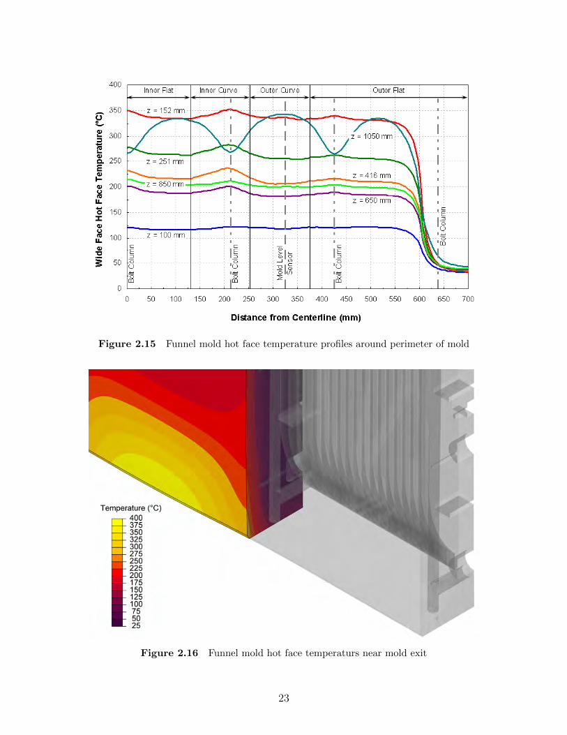
Figure 2.15 Funnel mold hot face temperature profiles around perimeter of mold

Figure 2.16 Funnel mold hot face temperaturs near mold exit

23

Figure 2.17 Funnel mold hot face temperature and distortion profiles for the narrowface mold

2.4.3 Thermocouple Temperature Validation

To further validate the model, the model predictions (top boxes) of thermocouple temper-

atures are compared against their measured values (bottom boxes) in Figure 2.14. Plant

data were selected for conditions close to those modeled, except that the strand width was

1300 mm, contrasting with 1200 mm in the model. The model therefore underpredicts signifi-

cantly the temperatures of the thermocouple column furthest from the centerline of the wide

face, and these temperatures are not given.

The measured thermocouple temperatures were time-averaged over 30 min of steady

casting and then adjusted to account for heat removal through the thermocouple wires. As

discussed in Section 3.4.3, the thermocouples act like long pin-fins, and the adjustment to

24

the thermocouple temperature to account for this effect is given in Equation (3.45). The

copper-constantan thermocouples used in this work with wire diameter DTC = 4 mm and

thermal conductivity kTC = 212 W/(m ·K) are adjusted using a gap between the mold and

thermocouple of size dgap = 0.01 mm and thermal conductivity of kgap = 1.25 W/(m ·K).

The wire convection coefficient hwire is taken as 5 kW/(m2 ·K) if the thermocouple passes

through water, or as 0.1 kW/(m2 ·K) if the thermocouple is only in ambient air. The ambient

temperature is taken from the cond model predictions of cooling water temperature if the

thermocouple passes through water, or as 25 ◦C if the thermocouple is only in ambient air.

Figure 2.14 specifies with an ‘a’ or a ‘w’ which thermocouples are adjusted for air and water.

Generally, the model and measurements match fairly well, usually within 10 ◦C (5%

error). The thermocouples on the narrow faces nearest mold exit are overpredicted, but this

observation is expected given that the cond model was calibrated for the wide face. Some

of the wide face thermocouple measurements showed considerable asymmetry (30 ◦C–40 ◦C)

between the plates on the inner and outer radius, so deviations from the modeling predictions

are expected at those locations. The outer-radius wide face measurements match much better

with the model predictions than the inner radius, suggesting a difference between inner- and

outer-radius (the outer-radius wide face generally had the higher temperatures). The larger

mismatches occur in the funnel region near the meniscus, so the shell might be losing contact

with the mold more on one side than on the other.

2.5 Conclusions

This chapter provides insight into the thermal behavior of steel continuous-casting molds

during steady casting, based on geometrically-accurate d finite-element analyses. The hot

face of the mold, regardless of the shape, should maintain a uniform temperature around

the perimeter to help reduce the occurrence of cracks in the mold and in the solidifying

steel. The geometric accuracy of the models in this chapter reveal variations in the hot face

temperature related to the spacing of the water channels, and in particular with the change

in cooling related to the water channels around the columns of bolt holes in the back of

the mold. Both a beam-blank mold and a funnel mold show that the hot face temperature

increases near mold exit because of the change in cooling pattern, which could lead to other

problems. This chapter demonstrated a method for calibrating thermocouple temperatures

to account for an air gap between the tip of the thermocouple and the mold, and for heat lost

along the thermocouple wires. The mold temperatures calculated in this chapter are used in

other, more complicated models of the continuous casting process in the following chapters.

25

CHAPTER 3

Reduced-Order Model of Mold Heat Transfer1

3.1 Introduction

This chapter presents a reduced-order model of mold heat transfer in the continuous cast-

ing of steel. The reduced-order model itself is based on a one-dimensional solution to the

heat-conduction equation, and the up-front cost of the reduced-order model is a single

three-dimensional finite-element calculation of a small portion of the exact mold geome-

try. This three-dimensional calculation is used to calibrate the geometric parameters in the

one-dimensional temperature model. Other features of the reduced-order model, namely the

cooling water temperature change and thermocouple temperatures, are derived in a consistent

manner with the one-dimensional solution. The reduced-order model calibration is demon-

strated for four actual continuous casting molds. Combined with models of solidification and

mold-metal interfacial phenomena, this accurate and efficient modeling tool can be applied

to gain insights into aspects of heat transfer in the continuous casting process.

“Reduced-order modeling” is a technique that seeks to reduce the complexity of a system

while robustly maintaining the relationship between inputs and outputs. After an up-front

cost to develop the model, a reduced-order model (rom) executes in a small fraction of the

time of a full-order model with nearly the same accuracy. This reduction of complexity occurs

by simplifying physical relationships, like linearizing or decoupling physical phenomena, or

reducing the degrees of freedom of a system. Least-squares regression is the simplest form

of model reduction: a large number of points are replaced by a few polynomial coefficients

that define a continuum. The one- or two-equation turbulence models commonly used

in computational fluid dynamics are a reduction of the complexity of the Navier–Stokes

equations, though the difficulty of solving the discretized partial differential equations (pdes)

remains. Reducing the degrees of freedom in such a pde discretization is the subject of

1Much of the work presented in this chapter has been published [31] or will appear in articles by theauthor and collaborators. R. J. O’Malley initially had the idea of correcting the geometric effect of the moldthermocouples, which was explored by M. M. Langeneckert [47]. J. Iwasaki later identified that additionalcorrections to the cond model were necessary, in particular to attain the correct temperature of the hotface. I. Hwang developed some computational tools that automate the calibration procedure for the moldgeometry. The content of this chapter, entirely the work of the author, builds upon the work of Langeneckertand Iwasaki to create a systematic procedure for calibrating the cond model of mold heat transfer.

26

recent literature; techniques like proper-orthogonal decomposition can provide a reduced

solution basis that carries most of the physics of the solution [2, 10]. Reduced-order modeling

techniques have been used for approximating the transfer function in the solution of ordinary

differential equations [73], circuit analysis and design [24], solid mechanics computations

for real-time graphics rendering [6], fluid mechanics computations [10], and many other

applications.

The back of a typical continuous slab-casting mold is shown in Figure 3.1. The mold is

assembled from four single-piece slabs of a copper alloy, e.g., CuBe or CuCrZr, with cooling

channels machined into the back side of the slab, shown in Figure 3.1. Pressurized water flows

through these channels at speeds near 10 m/s to remove more than 1 MW of power from the

solidifying steel. Casting machines track the total energy removed from the solidifying steel

by the mold, measured indirectly as the temperature change of the cooling water. Some molds

include a thin coating layer of nickel or chromium to reduce the wearing of the “hot face,”

i.e., the face of the mold in contact with the strand. Several bolt holes are machined into the

back side of the mold for mounting the mold into its support structure and water-delivery

system, collectively called the “waterbox.” Molds are instrumented with thermocouples,

either between the water channels or coaxially with the bolt holes, for online monitoring

of the casting process. The cooling water temperature change and mold thermocouple

temperatures are the key validation points for models of mold heat transfer.

Modeling heat transfer in the continuous casting process requires accurate incorporation

of the mold, the solidifying strand, and the interface between them. The behavior of the

material in the interface, a ceramic slag, governs the heat extraction from the strand [57, 58].

Continuous casting of steel or any other metal is a complicated process with many coupled

and nonlinear phenomena, and requires advanced modeling techniques to understand what

is important for the process. Most of the process phenomena are dependent upon the mold

heat transfer, e.g., the rate-dependent solidification shrinkage of the solid shell, the time-

dependent crystallization and flow of the interfacial slag, or the the multiphase turbulent

flow of the molten steel with a free surface and particle transport. Much of the previous work

on these three topics makes poor assumptions about mold heat transfer because modeling

these phenomena alone are challenging tasks.

The continuous casting literature has several examples of mold heat transfer models

with various levels of geometric complexity. Some of the models of mold heat transfer

investigate only phenomena related to mold heat transfer [11, 55, 81, 84, 97, 110], and others

use the calculated thermal behavior to drive the expansion of the mold in investigations

of mold distortion [33, 35, 53, 68, 69, 71, 80, 83, 98, 109, 113, 117]. Some models of the

27

wmold

ℓmold

dmold

xy

z

Mold Calibration Domain

WaterChannelsBolt Hole

Thermocouple Hole

FaceThermocouple

Hot Face

Figure 3.1 Back of a typical continuous casting mold showing the calibration domain

solidification shrinkage of the strand [27, 35, 116] and of the turbulent flow of the molten

steel [18, 62, 67] have included detailed models of mold heat transfer. Some analyses are

a part of an inverse model to calculate information about the heat extraction from the

strand [18, 19, 22, 54, 74, 102, 108, 111, 112]. The most complicated studies have combined

models of fluid flow, strand solidification and deformation, mold heat transfer, and mold

distortion [38, 39, 50, 51, 63]; these studies all mention the many difficulties of converging

these mutli-domain, multi-field, multi-physics models; cf. Chapter 5 for further discussion.

A continuous casting mold can be modeled in three dimensions, with as much geometric

detail required by the modeler. Sometimes models of this complexity are necessary to explore

the details of heat transfer with complicated-shaped molds [35, 39, 51, 110] and water

channels [31, 33, 97], or the thermal distortion of the mold. These detailed models reveal

the variation of temperature around geometric features like thermocouple holes and water

channels; cf. Chapter 2 for examples. The mold-only heat transfer simulations, even with

a fine mesh and full geometric detail [33, 35], require minutes to solve on modern computer

platforms; however, interfacing and iterating the mold simulations with other models is

computationally challenging. There is a need for a simple-but-accurate model of mold heat

transfer for use with more complicated simulations.

28

The geometry of the continuous casting process allows many phenomena to be modeled

reasonably well with a one-dimensional (d) assumption, particularly away from the corners

of the strand. The rom of mold heat transfer presented in this work is a part of the

process model cond [56], which is a d finite-difference model of the solidifying strand and

includes simple models of solidification microscale physics and lubrication and heat transfer

in the strand-mold interface. The cond model has been applied to several commercial

casters [58, 77, 84, 86], and the mold model has evolved from a d heat-conduction model

with several ad hoc corrections into the rom presented in this work.

The reduced-order model of mold heat transfer that is presented in Section 3.3 is based

on a d solution to the heat-conduction equation, and the up-front cost of the model is

to calibrate its parameters with a single small three-dimensional (d) finite-element model

of the physical mold, which is discussed in Section 3.2. This rom uses the physics of an

analytical solution, rather than a statistical technique, to provide a robust relationship

between the boundary conditions and the mold temperatures. The calibration of the rom is

discussed in Section 3.4, and then several examples are presented in Section 3.5. Section 3.6

shows calibration of the rom is insensitive to the boundary conditions, so the calibration

needs to be performed once per mold geometry.

3.2 Three-Dimensional Mold Model: Snapshot Model

Consider a small periodic and symmetric portion of the mold, shown in Figure 3.1. Analysis

of this domain serves as the “snapshot” model for the reduced-order model developed in this

work. The temperature in this d model of the mold T3D(x) is determined by solving the

steady heat-conduction equation subject to appropriate boundary conditions, as discussed

in Section 2.2. A uniform heat flux qhot is supplied to the mold hot face, and energy is

extracted from the water channel surfaces by a uniform convection condition with heat

transfer coefficient hwater and sink temperature Twater. All other faces are insulated, because

of symmetry or the assumption that negligible heat flows from the back of the mold. Any

other features of the mold, such as a coating layer, should be included in this snapshot

model. Modern computers can solve this linear heat conduction problem in minutes or less,

depending on mesh resolution.

The details of the heat transfer are computed with this small but fast and accurate model,

and then the results are used to calibrate the reduced-order model of mold heat transfer

presented in Section 3.3. The accurate d model essentially acts as a “microscale” model for

the faster d “macroscale” model. For the calibration of the rom, discussed in Section 3.3,

29

four temperatures are extracted from this small d model:

• the average hot face temperature, T3D,hot, which is used in calculations of the strand-

mold interfacial heat transfer,

• the average water channel surface temperature, T3D,c, which is needed to calculate

correctly the heat transfer coefficient of the water convection,

• the maximum water channel surface temperature, T3D,roots, which usually occurs at

the channel root, is used to evaluate the risk of boiling the cooling water, and

• the average thermocouple face temperature, T3D,TC, which is an important validation

point in models of mold heat transfer.

The averaging occurs over the appropriate surfaces indicated in Figure 3.1.

3.3 Reduced-Order Model of Mold Heat Transfer

This section discusses the reduced-order model of mold heat transfer in continuous casting

developed in this article. The reduced-order model is based on a solution to the d heat-

conduction equation.

3.3.1 One-Dimensional Heat Conduction Analysis

Scaling analysis [21] justifies the d assumption used in analyzing the mold heat transfer.

The scaled steady heat-conduction equation is

0 =∂2θmold

∂x∗2+

(dmold

wmold

)2∂2θmold

∂y∗2+

(dmold

`mold

)2∂2θmold

∂z∗2, (3.1)

where θmold =(Tmold − Twater

)/(Tmold,max − Twater

)is the mold temperature Tmold scaled

by the maximum mold temperature Tmold,max and cooling water bulk temperature Twater,

and x∗ = x/dmold, y∗ = y/wmold, and z∗ = z/`mold are the coordinates scaled by the mold

thickness dmold, width wmold, and length `mold. As illustrated in Figure 3.1, the aspect ratio

terms in Equation (3.1) are small, i.e., dmold/wmold � 1 and dmold/`mold � 1, so the terms

that they multiply can be neglected. This analysis indicates that the conduction through the

thickness of the mold, i.e., in the x-direction, is the dominant mode of heat transfer. The d

assumption is inaccurate near the liquid steel meniscus because of the large gradient of heat

flux in the casting (z) direction, so a higher-order model may be necessary in this region.

The mold in the reduced-order model is envisioned as a rectangular plate with thick-

ness dplate and thermal conductivity kmold, with a large number of rectangular water channels,

30

as shown in Figure 3.2. All water channels are identical with depth dc, width wc, and pitch pc.

The coating layer has thickness dcoat and thermal conductivity kcoat. Assuming that the

mold copper between the water channels acts as a heat-transfer fin, the “cold face” of the

mold, described in Section 3.3.2, is modeled as a convection condition with heat transfer

coefficient hcold and sink temperature Twater. The mold is analyzed easily as a number of d

thermal resistances, shown in Figure 3.3, with this treatment of the water channels.

The temperature in the mold T1D(x) is governed by the d heat-conduction equation,

0 =d2T1D

dx2, (3.2)

which has the general solution

T1D(x) = c1x+ c2, (3.3)

where x is the distance from the hot face, including the coating layer, and c1 and c2 are

constants of integration. The solidifying steel supplies a heat flux qhot > 0 to the hot face of

the mold at x = 0, which has a normal vector of n = −1, or

− kcoatdT1D

dx

∣∣∣∣x=0

(−1) = −qhot. (3.4)

The interface between the coating layer and mold copper at x = dcoat has continuous

temperature,

T1D

(d−coat

)= T1D

(d+

coat

), (3.5)

and continuous heat flux,

− kcoatdT1D

dx

∣∣∣∣x=d−coat

(+1) = −kmolddT1D

dx

∣∣∣∣x=d+

coat

(−1) . (3.6)

The cold face at x = dcoat + dplate, which has a normal vector of n = +1, has the convection

condition

− kmolddT1D

dx

∣∣∣∣x=dcoat+dplate

(+1) = hcold

(T1D(dcoat + dplate)− Twater

). (3.7)

Applying these boundary conditions gives the d temperature field as

T1D(x) =

Twater + qhot

(1

hcold

+dplate

kmold

+dcoat − xkcoat

)if 0 ≤ x ≤ dcoat

Twater + qhot

(1

hcold

+dplate + dcoat − x

kmold

)if dcoat ≤ x ≤ dcoat + dplate.

(3.8)

The d temperature solution is shown schematically in Figure 3.4.

31

pc

wc

dfoul

dmold

dc dplate dcoat

Fin

Tip

Base

Water Channel

Root Mold Plate

Fouling Layer

Coating Layer

y

x

qhot

Figure 3.2 Simplified mold geometry used for developing the reduced-order model

32

qhotdcoat

kcoat

dplate

kmold

1

hfins

/(1 − wc

pc

)

dfoul

kfoul

/wc

pc

1

hwater

/wc

pc

Twater

Figure 3.3 Thermal resistor model for the one-dimensional mold

Distance from Hot Face x

Tem

per

atu

reT

Thot

Tcold

Tfoul

Twater

Tfins

dc dplate

dfoul dcoat

Figure 3.4 One-dimensional model of mold temperatures

33

The temperature solution, Equation (3.8), is used to find the temperature at key locations

in the mold. The hot face temperature T1D,hot = T1D(0) is

T1D,hot = Twater + qhot

(1

hcold

+dplate

kmold

+dcoat

kcoat

), (3.9)

and the cold face temperature T1D,cold = T1D(dcoat + dplate) is

T1D,cold = Twater +qhot

hcold

. (3.10)

A thermocouple with depth dTC beneath the hot face has temperature T1D,TC = T1D(dTC), or

T1D,TC = Twater + qhot

(1

hcold

+dplate + dcoat − dTC

kmold

). (3.11)

The temperature solution also gives the heat transfer coefficient hmold that can be used to

model the thermal effect of the mold in other, more complicated models of the continuous

casting process,1

hmold

=1

hcold

+dplate

kmold

+dcoat

kcoat

, (3.12)

with Twater as the sink temperature.

3.3.2 Cold Face Model

The water flowing in the cooling channels causes a nominal heat transfer coefficient of hwater

that is modified to account for other phenomena in the water channels. The water convection

coefficient hwater itself is calculated with a forced-internal-flow empirical correlation, such as

the sleicher and rouse [89] model presented in Equation (2.7).

Heat is extracted at the cold face by convection along the roots of the channels, and by

combined conduction through the bulk of and convection along the lateral surfaces of the

fins. These two effects combine to provide a cold face heat transfer coefficient of

hcold =

(wc

pc

)hroots +

(1− wc

pc

)hfins, (3.13)

where hroots is the heat transfer coefficient for the root surfaces and hfins is the heat transfer

coefficient for the fins.

The heat transfer coefficient for the water channel roots hroots is the nominal hwater reduced

by the effects of a thin layer of fouling material, such as calcium carbonate or an organic

compound, with thickness dfoul and thermal conductivity kfoul according to

1

hroots

=1

hwater

+dfoul

kfoul

. (3.14)

34

The thickness of the fouling layer is assumed to be small compared to the channel depth,

i.e., dfoul/dc � 1, as to not affect significantly the flow of the cooling water. Additionally, as

the fouling layer thickness dfoul increases more heat flows into the fins, causing more d heat

transfer within the mold plate.

The mold copper between water channels is assumed to act as a rectangular fin with an

insulated tip, giving a heat transfer coefficient of

hfins = hwatertanh(b)√

Biwfins

, (3.15)

where the Biot number based on the fin half-width is

Biwfins=hwater

kmold

pc − wc

2, (3.16)

the Biot number based on the fin length is

Bidfins=hwater

kmold

dc, (3.17)

and b = Bidfins/√

Biwfinsis introduced for convenience. The fin tip is insulated because

of the assumption that all of the energy from the steel is removed by the cooling water.

Equation (3.15) was derived for a fin with uniform cross-section and material properties, and

for a thin fin, i.e., (pc − wc)/dc � 1. The fin aspect ratio is approximately 1/3 in practice,

so the d heat transfer within and at the base of the fin may be significant.

A needed quantity is the perimeter-average temperature of the water channel, Tc. The

temperature along the length of a rectangular fin Tfins(x′) is described by

Tfins − Twater

Tbase − Twater

=1

cosh(b)cosh

(b

(1− x′

dc

)), (3.18)

where x′ is the distance from the base of the fin. The perimeter-average temperature of

the rectangular water channel, having two sides of length dc with temperature described

by Equation (3.18), one side of length wc with uniform temperature Twater, and one side of

length wc with uniform temperature Tfoul, is

Tc =1

dc + wc

(wc

2Tfoul +

(wc

2+ dc

)Twater + dc

tanh(b)

b

(Tbase − Twater

)). (3.19)

The temperature at the base of the fin is taken as the cold face temperature from Equa-

tion (3.10), i.e., Tbase = T1D,cold. The temperature of the surface of the fouling layer Tfoul,

computed with the circuit mathematics for the d heat transfer model, is

Tfoul = Twater +qhot

hcold

hroots

hwater

, (3.20)

35

which reduces to the cold face temperature T1D,cold when dfoul = 0.

Boiling in the water channels should be avoided because of the possible reduction in

heat transfer and formation of fouling material. A simple evaluation of the risk of boiling is

to compare the water temperature, in particular at the channel roots, against the saturation

temperature of the water [31, 83]. Since the water in the mold is pressurized, the saturation

temperature of water Tsat,water(p) is computed with [37]

Tsat,water = 325.088 +D −√

(325.088−D)2 + 0.238 556, (3.21)

where

D =1

2

C√B2 + AC +B

103, (3.22)

A = (β − 0.923 517) (β − 16.1503) , (3.23)

B = 0.583 526 (β − 0.386 723) (β + 10.6869) , (3.24)

C = 0.724 213 (β − 0.121 989) (β + 4.585 53) , (3.25)

β = 4√p. (3.26)

Equation (3.21) expects the absolute pressure p in MPa and gives the saturation temperature

in K. This model is valid for 0.611× 10−3 MPa ≤ p ≤ 22.0 MPa, which is satisfied in practice.

An interesting digression is to observe that the cold face heat transfer coefficient hcold given

in Equation (3.13), without a fouling layer and with constant hwater, has the maximum value

of 53hwater at a channel pitch of pc = 3

4kmold

hwater≈ 9 mm, a channel width of wc = 1

4kmold

hwater≈ 3 mm,

and a channel depth of dc = atanh(χ) 12kmold

hwater≈ 21 mm, where 0.95 ≤ χ < 1.0 is a tolerance

on the asymptote of the hyperbolic tangent. These values of channel geometry provide an

intelligent starting point for further work on optimizing mold geometry, though efficient heat

extraction is but one goal of mold design. Other mold design goals may include:

• optimizing, but generally maximizing, the mold hot face temperature for best steel

quality,

• minimizing the hot face temperature variation around the perimeter of the mold,

across all four mold pieces, to reduce the formation of longitudinal cracks both in the

steel and in the mold,

• avoiding the water boiling in the channels, as discussed above,

• minimizing the thermomechanical stress concentrations near the water channel roots

to extend the mold service life,

• minimizing the hot face temperature, to avoid accelerated creep rates and reduce

thermomechanical fatigue loading, to extend the mold service life,

36

• maximizing the mold plate thickness, to increase the mold service life and to provide

a safety factor against mold cracking,

• minimizing the volume of copper of the mold, for low material cost,

• minimizing the total channel cross-sectional area, or at least the channel cross-sectional

area per unit width of the mold, for low manufacturing cost, and

• maximizing the individual channel cross-sectional areas to reduce the pressure differ-

ence required to drive the water flow, for low operating cost.

Getting the steel as cold as possible as quickly as possible is not a goal of mold design.

Reducing the manufacturing and operating costs of the mold are minor goals compared to

producing high-quality steel. The rom developed in this work can be used to explore some

of these design issues.

3.3.3 Cooling Water Temperature Change

The temperature change of the cooling water is an important quantity in the validation of

mold heat transfer models because it indirectly measures the heat removed from the steel

by the mold. This section presents the calculation of the temperature change of the cooling

water in the reduced-order model, in a manner that is consistent with the rest of the model.

Assuming that the water moves mostly in the axial (z) direction of the water channel

with average speed vwater, the scaled [21] steady energy equation is

∂θwater

∂z∗=

1

PewaterDh,c

`c

(∂2θwater

∂x∗2+∂2θwater

∂y∗2+

(Dh,c

`c

)2∂2θwater

∂z∗2

), (3.27)

where θwater = (Twater − Twater,min) / (Twater,max − Twater,min) is the temperature of the wa-

ter Twater scaled by the largest and smallest water temperatures in the water channel Twater,max

and Twater,min, x∗ = x/Dh,c, y∗ = y/Dh,c, and z∗ = z/`c are the coordinates scaled by the

hydraulic diameter Dh,c and length `c of the water channel, Pewater = vwaterDh,c/αwater is

the Peclet number of the flow in the water channel, and αwater = kwater/ρwatercp,water is the

thermal diffusivity of the water. Equation (3.27) indicates that the heat conducted in the

axial (z) direction is negligible relative to the heat conducted in the transverse directions

because of the small aspect ratio of the channel, i.e., Dh,c/`c � 1. Further, since the aspect-

ratio–modified Peclet number is large, i.e., PewaterDh,c

`c� 1, the heat conduction is negligible

relative to the energy transported by the bulk motion of the water. Equation (3.27) then

indicates that the water temperature is uniform over the entire channel, so an alternative

approach must be used to analyze the temperature change of the water.

37

qhot

qwater

qwater

∆z

pc

Mold

Water

xy

z

Figure 3.5 Domain for analyzing the cooling water temperature change

Consider a transverse slice with thickness ∆z > 0 of a water channel and the surrounding

mold, as shown in Figure 3.5. The integral form of the steady energy equation for the water,

assuming no boiling, in the transverse slice is

∫

Vwater

ρwatercp,watervwater∂Twater

∂zdV = −

∫

Ac

−qwater dA, (3.28)

where Vwater is the volume of the slice of water, Ac is the surface area of the water channel

in the slice, and qwater > 0 is the heat flux into the water. All heat supplied to the mold

is assumed to be removed by the cooling water, so the integral form of the steady energy

equation for the mold in the transverse slice is

0 = −∫

Ahot

−qhot dA−∫

Ac

qwater dA, (3.29)

where the area of the hot face in the transverse slice is Ahot = pc∆z. If the heat flux on the

hot face is uniform across the slice, then the heat input to the water is

∫

Ac

qwater dA = qhotpc∆z (3.30)

38

regardless of the shape of the water channel. The hot face heat flux qhot is uniform for an

arbitrarily small ∆z and a water channel width-to-pitch ratio wc/pc greater than some as yet

unknown value. The volume integral over the water in Equation (3.28) is avoided by defining

the water bulk temperature Twater as the temperature that satisfies

ρwater

(Twater

)cp,water

(Twater

)vwaterTwaterAc =

∫

Ac

ρwatercp,watervwaterTwater dA, (3.31)

i.e., Twater(z) is the internal-energy–weighted average temperature over a plane perpendicular

to the flow of the water with cross-sectional area Ac. Equation (3.31) allows the volume

integral in Equation (3.28) to be evaluated for small ∆z as

∫

Vwater

ρwatercp,watervwater∂Twater

∂zdV = ρwatercp,watervwater

dTwater

dzAc∆z, (3.32)

with ρwater and cp,water on the right-hand side evaluated at Twater. Combining Equations (3.28),

(3.30), and (3.32) and dividing out the ∆z gives the differential equation that describes the

evolution of the water bulk temperature in one channel as

ρwatercp,watervwaterdTwater

dzAc = qhotpc. (3.33)

The above arguments are extended to find the temperature change of all of the cooling

water in the mold. The heat flux from the steel is applied over the width of the strand wstrand

rather than a single channel pitch. The heat leaves the mold through all water channels with

total cross-sectional area Ac,total, regardless of channel shape and pitch; however, the water

speed in each channel must be about the average value vwater. The temperature evolution of

the total water then is described by

ρwatercp,watervwaterdTwater

dzAc,total = qhotwstrand. (3.34)

The water temperature at an arbitrary distance down the mold z is found by numerical

integration of Equation (3.34),

Twater(z) = Twater(0) +

∫ z

0

1

vwater

wstrand

Ac,total

qhot

ρwatercp,water

dz′, (3.35)

where Twater(0) is the water temperature at the top of the mold, a value measured in the plant.

The temperature of the water at the bottom of the mold Twater(`mold) is the measurement

from the plant that the reduced-order model must match as part of the heat flux calibration

procedure. This calculation of water temperature change works equally well in counterflow

configurations, where the cooling water flows in the direction opposite to the casting direction,

but with vwater < 0.

39

3.4 Reduced-Order Model Parameter Calibration

The thirteen parameters in the reduced-order model of mold heat transfer presented in

Section 3.3 are the

• boundary conditions: the hot face heat flux qhot, and the water heat transfer coeffi-

cient hwater and bulk temperature Twater,

• material properties: the coating, mold, and fouling thermal conductivities kcoat, kmold,

and kfoul, and the

• geometries: the coating, mold plate, and fouling thicknesses dcoat, dplate, and dfoul, the

thermocouple position dTC, and the water channel width wc, depth dc, and pitch pc.

For a given problem, the non-geometric parameters, i.e., the material properties and the

boundary conditions are fixed parameters. Some of the geometric parameters are taken

as the calibration parameters of the rom because of the assumptions about the nature of

the heat flow in the simplified model, and because these parameters allow enough leeway

for the rom to be robust with respect to changes in the non-geometric parameters, which

is explored in Section 3.6. The coating and fouling layer thicknesses dcoat and dfoul are taken

as fixed parameters because they are so thin that these layers act as d thermal resistances

regardless of the complexity of the model. The five remaining geometric parameters, the

mold plate thickness dplate, the thermocouple depth dTC, and the channel width wc, depth dc,

and pitch pc, are calibrated in this section so that the reduced-order model of the mold has

the same thermal characteristics of the physical mold and can match key temperatures in

the d model discussed in Section 3.2.

3.4.1 Water Channel Geometry

The reduced-order model water channel geometry is calibrated by appealing to physical

principles. The water channels in the rom must have the same cross-sectional area as the

physical channels Aphysical, i.e.,

wcdc = Aphysical, (3.36)

to maintain the mass flow rate of the cooling water. The water channels in the rom also

must have the same hydraulic diameter as the physical channels Dh,physical, i.e.,

2wcdc

wc + dc

= Dh,physical, (3.37)

40

to maintain the value of the heat transfer coefficient hwater from Equation (2.7). Solving

Equations (3.36) and (3.37) together gives the rom channel width wc and depth dc as

wc, dc =Aphysical

Dh,physical

1±

√1−

D2h,physical

Aphysical

. (3.38)

Both solutions of Equation (3.38) are real and positive if Aphysical ≥ D2h,physical. The aspect

ratio of the physical channels determines which solution is wc and which is dc, subject to

wc < pc. Some molds employ channels with different geometries; in this case the values of

Aphysical and Dh,physical are taken as their respective averages over all channels in the mold.

The limitation of Aphysical ≥ D2h,physical precludes molds with only circular channels. In

this case, the rom channel width is defined as the width of the square that circumscribes

the circle, wc = Dphysical, and the depth of the channel is calculated to match the cross-

sectional area, i.e., dc = π4Dphysical. This approach matches the cross-sectional area but gives

a hydraulic diameter of Dh,c ≈ 0.88Dphysical. Taking the d channel width to be that of the

square that inscribes the circle gives Dh,c ≈ 0.86Dphysical. The previous approach [84] that

used wc = 23Dphysical gives Dh,c ≈ 0.85Dphysical. Each of these approaches over-predict the

heat transfer coefficient hwater from Equation (2.7) by about 3%, and the larger the channel

diameter the smaller the error.

The rom channel pitch pc is calibrated by requiring that the simulated and physical

molds have the same amount of water flowing per unit width of the mold, i.e.,

Ac

pc

=Ac,total

wmold

, (3.39)

where the rom water channel cross-sectional area Ac = wcdc is calculated with the calibrated

dimensions from Equation (3.38). The mold width wmold and total channel cross-sectional

area Ac,total used in this calculation should be based on regions away from the ends of the

mold; ideally, this calculation is based upon the geometry of the d calibration domain

discussed in Section 3.2. The rom channel pitch was determined in previous work [31] from

the slope of the best-fit line through the function describing the cumulative water channel

cross-sectional area across the width of the mold, as shown in Figure 3.6, which is based on

the example Mold d presented in Section 3.5. Equation (3.39) gives a simple but accurate,

within about 3% depending on the channel geometry, approximation of this best-fit line.

3.4.2 Mold Plate Thickness

The mold plate thickness in the rom is calibrated by forcing the temperature at specific

locations in the d model to match the corresponding temperatures in the d model subject to

41

0 10 20 30 40 50 60 70 80 90 100 110

Distance from Mold Centerline (mm)

0

100

200

300

400

500C

um

ula

tive

Wat

erC

han

nel

Cro

ss-S

ecti

onal

Are

a(m

m2)

Slope of best-fit line = 4.556 mm2/mmAc,total/wmold = 4.570 mm2/mm

Figure 3.6 Cumulative water channel area across the Mold d calibration domain

identical boundary conditions and material properties. Before proceeding, choose reasonable

values for the non-geometric model parameters k�mold, q�hot, h�water, T

�water, d

�coat, k

�coat, d

�foul, and

k�foul to be used in both the d and the d models.

The calibrated mold plate thickness dplate is found by requiring the d hot face temperature

to be the average hot face temperature from the d finite-element model, i.e., T1D,hot = T3D,hot.

Manipulating the expression for the d hot face temperature, Equation (3.9), gives a mold

plate thickness of

dplate =k�mold

q�hot

(T3D,hot − T �water

)− k�mold

(1

h�cold

+d�coat

k�coat

), (3.40)

where h�cold is calculated with Equation (3.13) using the calibrated channel geometry from

Section 3.4.1. Some phenomena related to strand-mold interfacial heat transfer depend

on the mold hot face temperature, and this calibrated plate thickness ensures that T1D,hot

is computed accurately.

Changing the thickness of the mold plate then requires concordant redefinition of the cold

face. Two “cold face” positions are calibrated for the rom: one for the average water channel

surface temperature, dchannels, and one for the maximum water channel surface temperature,

droots, respectively used to calculate the water heat transfer coefficient with Equation (2.7),

42

and to evaluate the risk of boiling with the saturation temperature, Equation (3.21). Following

similar arguments as in calibrating the mold plate thickness gives

dchannels =k�mold

q�hot

(T3D,hot − T3D,c) + d�coat

(1− k�mold

k�coat

), (3.41)

where T3D,c is the average temperature of the channel surfaces in the d calibration domain,

and

droots =k�mold

q�hot

(T3D,hot − T3D,roots) + d�coat

(1− k�mold

k�coat

), (3.42)

where T3D,roots is the maximum temperature of the channel roots in the d calibration domain.

This idea of “multiple cold faces” can be extended as necessary, depending on the interests

of the modeler.

3.4.3 Mold Thermocouples

The mold thermocouples in the rom are calibrated to account for the geometric effect of the

thermocouple bore, and to account for the heat lost along the long thermocouple wires. The

geometric effect can be significant: the temperature from Equation (3.11) under-predicts the

thermocouple temperature from the d model, by as much as 50 ◦C [47, 84], or about 25%,

depending on the geometry. Following similar arguments as in calibrating the mold plate

thickness, the calibrated thermocouple position dTC is found by manipulating Equation (3.11)

with T1D,TC = T3D,TC, giving

dTC =k�mold

q�hot

(T3D,hot − T3D,TC) + d�coat

(1− k�mold

k�coat

). (3.43)

Using the result of Equation (3.43) corrects the geometric inaccuracies of the thermocouple

temperature, but in practice is insufficient alone to match thermocouple measurements.

Measured thermocouple temperatures often read low because of the contact resistance between

the thermocouple bead and the appropriate surface on the mold. Heat also is lost through

conduction and convection along the length of the thermocouple wires, especially if the wires

are long and well-cooled. Assuming that the thermocouple wires behave as long circular

pin-fins, the heat loss is

qTC =kTC

DTC/2

√hwireDTC

kTC

(TTC − Tamb) , (3.44)

where DTC and kTC are the diameter and the thermal conductivity of the thermocouple wire,

which is submersed in a fluid of temperature Tamb that causes a convection coefficient of hwire.

43

The wire heat transfer coefficient hwire is intended to be a tuning parameter, and should be

about 5 kW/(m2 ·K) if the ambient medium is water or about 0.1 kW/(m2 ·K) for air. Since

the heat leaving the mold through the thermocouples is small relative to the heat leaving

through the water channels, this heat lost along the thermocouple wires is treated as a local

adjustment to the thermocouple temperature,

T ′TC = TTC + qTCdgap

kgap

, (3.45)

where TTC is the predicted thermocouple temperature from Equation (3.11) using the cal-

ibrated thermocouple depth dTC from Equation (3.43), and dgap and kgap are the size and

the thermal conductivity of the gap between the thermocouple and the mold copper. The

thermal conductivity of the gap should be about 1.25 W/(m ·K) for a thermal paste or about

0.04 W/(m ·K) for dry air. The gap size typically is on the order of 0.01 mm to 0.1 mm,

and is used as a tuning parameter in the heat flux calibration procedure. This approach of

calibrating mold thermocouple temperatures is used in Chapter 2.

3.5 Example Mold Geometries

This section presents the determination of the reduced-order model parameters for four wide

face mold geometries. This work employs the commercial finite-element software abaqus [1]

for analyzing the d calibration domains. Molds a and b [47] are for conventional “thick-slab”

molds, Mold c [84] is for a thin-slab funnel mold, and Mold d [31] is for a thin-slab mold

without a funnel. All molds do not employ coating layers. Slices through the calibration

domains at the center of the thermocouple are shown in Figures 3.7 through 3.10. These

figures also give the d model results that are necessary for the calibration calculations, and

the calibrated geometries for the reduced-order models of these molds. Water channels on a

symmetry plane, as on Molds a and b, have weights of 0.5 in the averaging calculations.

The severity of the adjustment to the channel geometry depends on the shapes and

distribution of channels in the physical mold. The mold plate thickness and its relatives are

about 10% different from the blueprint dimensions. Table 3.1 compares the temperatures

from the “uncalibrated” d heat-transfer model of the mold using the blueprint geometry,

and from the calibrated reduced-order model. The rom matches the temperatures from the

d model by construction, and the uncalibrated model under-predicts these temperatures

by as much as 26%. The thermocouple temperatures all are significantly underpredicted by

the uncalibrated model. Some molds, such as Mold d, are modeled reasonably well by the

uncalibrated model.

44

24

11

77

30

5

35

16 22 6

13

5

10

ALL DIMENSIONS IN MM

4 3 2

BH

TC

75

100

125

150

175

200

225

250

275

300 ◦C

k�mold = 315 W/(m ·K)

q�hot = 2500 kW/m2

h�water = 54 kW/(m2 ·K)

T �water = 35 ◦C

T3D,hot = 323.8 ◦C

T3D,TC = 172.0 ◦C

ChannelAc Dh,c Tc Troots

mm2 mm ◦C ◦C

1 56.14 7.631 71.86 107.02 80.0 7.619 59.20 79.793 80.0 7.619 60.52 80.614 80.0 7.619 62.50 80.70

Total 256.1rom 73.18 7.623 63.52 107.0

Modelwc dc pc dplate droots dchannels dTC

mm mm mm mm mm mm mm

Uncalibrated rom 16.0 5.0 22.0 30.0 24.0Calibrated rom 13.96 5.243 22.0 30.46 27.32 32.79 19.13

Figure 3.7 Calibration domain geometry, conditions, and results for Mold a [47]

45

22

5

18

77.5

27

18

45

5 15 6

15

210.75

ALL DIMENSIONS IN MM

5 4 3 2

BH

TC

50

75

100

125

150

175 ◦C

k�mold = 364 W/(m ·K)

q�hot = 1750 kW/m2

h�water = 45 kW/(m2 ·K)

T �water = 25 ◦C

T3D,hot = 192.6 ◦C

T3D,TC = 103.8 ◦C

ChannelAc Dh,c Tc Troots

mm2 mm ◦C ◦C

1 105.0 8.077 44.78 72.542 90.0 7.826 37.93 59.843 90.0 7.826 38.33 60.374 90.0 7.826 38.35 60.405 90.0 7.826 37.72 60.43

Total 420.0rom 93.33 7.882 39.42 72.54

Modelwc dc pc dplate droots dchannels dTC

mm mm mm mm mm mm mm

Uncalibrated rom 5.0 18.0 15.0 27.0 22.0Calibrated rom 4.994 18.69 17.22 27.51 24.98 31.87 18.48

Figure 3.8 Calibration domain geometry, conditions, and results for Mold b [47]

46

15

25

75

20.52

115

95 10

20

15

11

27.5

10

ALL DIMENSIONS IN MM

2345678910

BH

TC

COPPER MOLD INSERT

NOT INCLUDED IN ANALYSIS

75

100

125150175200225250

275 ◦C

k�mold = 350 W/(m ·K)

q�hot = 3000 kW/m2

h�water = 36 kW/(m2 ·K)

T �water = 40 ◦C

T3D,hot = 282.5 ◦C

T3D,TC = 179.6 ◦C

ChannelAc Dh,c Tc Troots

mm2 mm ◦C ◦C

1 78.54 10.0 91.18 124.12 72.32 7.642 72.04 115.93 72.32 7.642 63.58 109.34 72.32 7.642 62.85 107.45 72.32 7.642 62.52 106.46 72.32 7.642 62.37 105.97 72.32 7.642 62.24 105.58 72.32 7.642 62.20 105.59 72.32 7.642 62.16 105.410 72.32 7.642 62.17 105.3

Total 729.4rom 72.94 7.878 66.33 124.1

Modelwc dc pc dplate droots dchannels dTC

mm mm mm mm mm mm mm

Uncalibrated rom 5.0 14.0 10.0 21.0 15.0Calibrated rom 5.682 12.84 11.50 21.37 18.47 25.22 12.01

Figure 3.9 Calibration domain geometry, conditions, and results for Mold c [84]

47

40

43.85

108

16

6 5 5 5 5 6

22

1 62 3 4 5

9.4 18.1 17.7 17.6 17.8 18.1 9.3

ALL DIMENSIONS IN MM WATER CHANNEL PITCHES REFLECT GEOMETRY AWAY FROM THERMOCOUPLE HOLE

TC

75

100

125

150

175

200

225 ◦C

k�mold = 340 W/(m ·K)

q�hot = 2100 kW/m2

h�water = 32.5 kW/(m2 ·K)

T �water = 31 ◦C

T3D,hot = 245.7 ◦C

T3D,TC = 146.7 ◦C

ChannelAc Dh,c Tc Troots

mm2 mm ◦C ◦C

1 92.14 8.897 60.64 96.652 77.32 7.760 62.39 96.763 77.32 7.760 57.95 93.574 77.32 7.760 55.34 90.695 77.32 7.760 57.53 92.356 92.14 8.897 60.02 95.47

Total 493.5rom 82.26 8.139 58.98 96.76

Modelwc dc pc dplate droots dchannels dTC

mm mm mm mm mm mm mm

Uncalibrated rom 5.333 15.0 18.4 25.0 18.0Calibrated rom 5.647 14.57 18.0 25.75 24.12 30.24 16.03

Figure 3.10 Calibration domain geometry, conditions, and results for Mold d [31]

48

Table 3.1 Example mold geometry temperatures

Temperature (◦C)Mold a [47] Mold b [47] Mold c [84] Mold d [31]

Uncalibrated Calibrated Uncalibrated Calibrated Uncalibrated Calibrated Uncalibrated Calibrated

Hot face, Thot 317.5 323.8 187.9 192.6 276.3 282.5 242.1 245.7Cold face, Tcold 79.36 58.09 96.33 87.67Channel max., Troots 107.0 72.54 124.1 96.76Channel avg., Tc 59.55 63.52 37.65 39.42 62.30 66.33 60.32 58.98Thermocouple, TTC 127.0 172.0 82.12 103.8 147.8 179.6 130.9 146.7

49

3.6 Sensitivity of Mold Geometry Calibrations to Model Parameters

The calibration procedure evidently is insensitive to the non-geometric model parameters. For

simplicity, take dcoat = 0 and dfoul = 0. The derivative of the one-dimensional temperature

solution, Equation (3.8), with respect to the heat load is

∂T1D

∂qhot

=

(1

hcold

+L

kmold

)+

(qhot

kmold

∂L

∂qhot

). (3.46)

The second term arises because of the dependence of the calibrated dimension L upon the hot

face heat flux; this term must be small relative to the first term for the calibration process

to be insensitive to qhot, or that∣∣∣∣∂L

∂qhot

∣∣∣∣�kmold

qhothcold

+L

qhot

. (3.47)

The conditions for insensitivity of the calibration process for the other parameters are∣∣∣∣∂L

∂kmold

∣∣∣∣�L

kmold

, (3.48)

∣∣∣∣∂L

∂hwater

∣∣∣∣�kmold

h2cold

((wc

pc

)+

(1− wc

pc

)(tanh(b) + b

(1− tanh2(b)

)

2√

Biwfins

)), (3.49)

∣∣∣∣∂L

∂Twater

∣∣∣∣�kmold

qhot

. (3.50)

The sensitivity of the calibrated dimensions to the model parameters are evaluated with

these conditions.

Consider Mold a in Section 3.5; Figure 3.11 presents the results of a numerical experiment

that investigates the sensitivity of the calibrated mold plate thickness with respect to the

four non-geometric parameters over a wide range of values. The other molds in Section 3.5

produce similar results. The value of dplate is

• not at all sensitive to the heat load q�hot: the maximum derivative with respect to q�hot

is 7× 10−10, which is many orders of magnitude smaller than the limit predicted by

Equation (3.47),

• weakly sensitive to the mold thermal conductivity k�mold: and the maximum derivative

with respect to k�mold is 2.5× 10−3, which is 5% or less of the limit predicted by

Equation (3.48),

• somewhat sensitive to the water heat transfer coefficient h�water and bulk tempera-

ture T �water: the derivatives with respect to these variables are about 30% of the limits

predicted by Equations (3.49) and (3.50).

50

0 1 2 3 4 5 6 7 8

Hot Face Heat Flux q�hot (MW/m2)

0.00

0.01

0.02

0.03

0.04

0.05

0.06

0.07

0.08∣ ∣ ∣ ∣∂d

pla

te

∂q� h

ot

∣ ∣ ∣ ∣(m

3/M

W) Numerical Experiment

Insensitivity Criterion

0 100 200 300 400 500 600 700 800

Mold Thermal Conductivity k�mold (W/(m ·K))

0.0

0.1

0.2

0.3

0.4

0.5

0.6

0.7

0.8

∣ ∣ ∣ ∣∂d

pla

te

∂k� m

old

∣ ∣ ∣ ∣(m

2·K

/kW

)

0 10 20 30 40 50 60 70 80 90

Water HTC h�water (kW/(m2 ·K))

0.0

0.2

0.4

0.6

0.8

1.0

1.2

1.4

∣ ∣ ∣ ∣∂d

pla

te

∂h� w

ate

r

∣ ∣ ∣ ∣(m

3·K

/MW

)

0 10 20 30 40 50 60 70 80

Water Bulk Temperature T �water (◦C)

0.00

0.02

0.04

0.06

0.08

0.10

0.12

0.14

∣ ∣ ∣ ∣∂d

pla

te

∂T� wate

r

∣ ∣ ∣ ∣(m

m/K

)

Figure 3.11 Sensitivity of calibrated dplate to non-geometric rom parameters

As h�water decreases the derivative increases, and by h�water = 27 kW/(m2 ·K) the derivative

is 40% of the limit predicted by Equation (3.49). These lower values of hwater are valid

and feasible predictions from Equation (2.7) at lower water speeds. Reasonable accuracy

is attained from the rom by calibrating it with values of h�water and T �water that represent

averages of their ranges encountered in the plant.

3.7 Conclusions

A reduced-order model has been developed by calibrating some of the parameters in a sim-

ple analytical solution that contains the physics of the problem. The methodology has

been demonstrated specifically for mold heat transfer in continuous casting, and has created

a rigorous procedure for calibrating the geometric parameters for the mold. The “blueprint”

values of the mold geometry are changed by about 10% in the reduced-order model to com-

pensate for multi-dimensional heat transfer. This approach is insensitive to the boundary

conditions, so the model calibration procedure needs to be performed once per mold geometry.

Once this geometric calibration is performed, other more complicated models of continuous

casting can include accurate mold heat transfer with negligible computational cost.

51

CHAPTER 4

Steady-State Mechanical Behavior of the Mold1

4.1 Introduction

The thermal distortion of the continuous casting mold from room temperature to steady

operating temperatures can influence the behavior of the solidifying steel strand in many ways,

but likely the most important of these is the narrow-face (nf) taper. The thermo-mechanical

behavior for steady casting conditions has been explored for billet molds [50, 80, 82, 83, 109,

113], conventional thick-slab molds [53, 98, 117], and thin-slab molds with [63, 68, 69] and

without [68, 69] a funnel. Each mold shape has distinctive thermo-mechanical behavior, but

in general, these studies have revealed the importance of the waterbox on the mechanical

behavior of the system [98], and the importance of mold distortion on mold taper [80, 113],

mold cracks [63, 69], and steel strand cracks [50, 83]. Experimental measurements of the

mechanical behavior of molds during casting are rare; a few studies measured the wide face

waterbox shape with linear displacement transducers [13, 64, 65].

Mold distortion is less severe with lower mold temperatures, such as caused by lower

casting speeds [50, 80] or thinner mold plates [53, 80]. Coating layers have little influence on

the mechanical behavior of the mold [53] because they are so thin. The highest temperature

generally is found just below the meniscus, and operating with a metal level near a row of

bolts increases inelastic deformation of the copper near the hot face [80].

Many previous mold distortion models assume elastic behavior; incorporating inelastic

behavior of the mold copper is needed to predict residual stresses and residual distortion,

but does not significantly affect the mold shape during operation [63]. The previous models

have oversimplified the bolts and clamping, mold–mold and mold–waterbox contact, and the

mold and waterbox geometry. A complete quantitative analysis of thermal distortion during

operation of a continuous-casting mold, including realistic heat transfer, all of the important

geometric details, proper constraints, and validation with plant measurements, has not yet

been performed, and is the aim of this study.

1Much of the work presented in this chapter has been published by the author, for beam-blank molds [35]and for funnel molds [33, 34]. Beyond the content of these articles, this chapter contains an updated literaturereview and some details that were not included in the original publications. The measurements presented inthis chapter were provided by G. Abbel, A. Chown, R. Schimmel, and H. Visser at Tata Steel.

52

4.2 Model Description

The mechanical behavior of the mold and waterbox pieces is governed by the quasi-static

conservation of momentum,

0 = ∇ · � + b, (4.1)

where � is the Cauchy stress tensor and b is the body force density vector. The strains

experienced by the mold and waterbox are small, so a linearized description of motion

is adopted with total strain tensor

" =1

2

(∇u +∇u>

), (4.2)

which decomposes additively into elastic and thermal parts, i.e.,

" = "el + "th. (4.3)

The mold and waterbox are composed of isotropic polycrystalline copper and steel, so the

stress tensor is related to the elastic strain tensor with hooke’s law,

� = CCC : "el, (4.4)

where the components of the fourth-rank elastic stiffness tensor CCC are

Cijk` =

(κ− 2

3µ

)δijδk` + µ (δikδjl + δi`δkj) , (4.5)

where κ and µ are the isotropic bulk and shear moduli and δij is the kroenecker delta.

The thermal strain tensor is

"th = α (T − Tref) I, (4.6)

where α is the isotropic coefficient of thermal expansion based on reference temperature Tref ,

and I is the second-rank identity tensor.

Symmetry planes on the mold and waterbox have no normal displacement,

u · n = 0, (4.7)

and no tangential traction,

(I − n ⊗ n) · t = 0, (4.8)

where t = �> · n is the traction vector on the surface. Contacting surfaces between the mold

and waterbox or between the wide and narrow faces of the mold move together or form gaps

according to nonlinear conditions. Any point on the “master” surface with normal vector n

53

is nearest to some point on the “slave” surface, and the relative position between them is xrel.

The normal component of this relative position, dgap = xrel · n, is the size of the gap between

the surfaces. If the surfaces are not in contact, i.e., dgap > 0, then they are free of tractions,

t = 0. (4.9)

If the surfaces are in contact, i.e., dgap = 0, then they move with a relative velocity vrel that

has no normal component,

vrel · n = 0, (4.10)

and a tangential traction that follows the coulomb law,

(I − n ⊗ n) · t = −η (t · n)vrel

‖vrel‖2

, (4.11)

where η is the coefficient of friction, and the interfacial dissipation t · vrel is maximum. This

contact model [1] is described as “hard” because the contact pressure pc = t · n follows

pc = 0 (4.12)

if the surfaces are not in contact, i.e., dgap > 0, and

dgap = 0 (4.13)

if the surfaces are in contact, i.e., pc > 0. Mechanical contact is cast as a variational

problem [1] that finds the gap size dgap as

dgapn = xslave − xmaster (4.14)

subject to orthogonality with the two vectors t1 and t2 that are tangent to the direction of

sliding, i.e.,

t1 · (xslave − xmaster) = 0 (4.15)

t2 · (xslave − xmaster) = 0, (4.16)

where xmaster is a point constrained to lie on the master surface, i.e., a finite-element face, and

xslave is the nearest point on the slave surface, and the tangent vectors are computed from the

incremental motion across a time step. If the surfaces are in contact then the contact pressure

is introduced as a lagrange multiplier that enforces dgap = 0, i.e., Π = pc (xslave − xmaster)·n.

The hot face of the molds are supplied the traction

t = −pfn, (4.17)

54

to model the effect of ferrostatic pressure, where the applied pressure pf increases with

distance below the top of the liquid steel according to

pf =

{0 if z ≤ zmen

ρsteelg (z − zmen) if zmen ≤ z, (4.18)

where zmen is the position of the meniscus below the top of the mold, ρsteel is the mass

density of the liquid steel, and g is the acceleration due to gravity. The traction specified by

Equation (4.17) assumes that the dynamic pressure and skin friction of the molten steel have

negligible effect on the behavior of the mold. Strictly, the pressure distribution described

by Equation (4.18) is valid for the inside surface of the solidifying shell, but the ferrostatic

pressure is assumed to transmit perfectly through the solidifying steel and slag layers to the

mold hot faces. The ferrostatic pressure is applied only on the “active” hot face in contact

with the strand, from the meniscus to mold exit and in between the mold pieces.

As mentioned in Section 2.2, the waterbox is thermally inert, which decouples the thermal

and mechanical problems. Negligible heat is assumed to flow between the mold pieces because

the distortion opens an air gap along most of their originally-mating faces, as discussed

later. For the model of mold distortion, the waterbox is specified as isothermal at ambient

temperature, and the mold temperature fields are taken from the work presented in Chapter 2.

These temperatures drive the mechanical problem relative to an initial stress-free state at a

uniform temperature of T0, except for the mold bolts, which are described in Section 4.3.

The finite-element method is employed to solve this mechanical boundary-value problem,

using the commercial software abaqus [1]. The molds and waterboxes are modeled with

complete geometric detail, including the mold plates, water channels, bolts, bolt holes, tie-

rods, and waterboxes, as discussed in Sections A.1 and A.2. Only one symmetric fourth of

the assembly is modeled for computational efficiency. The domains are discretized with a

mix of “fully-integrated” linear 4-node tetrahedral, 6-node wedge, and 8-node hexahedral

elements (abaqus continuum elements cd, cd, and cd). Numerical experiments with

these elements in similar thermo-mechanical problems [1] has shown them quite capable of

matching analytical solutions, so numerical artifacts are of little concern. The ferrostatic

pressure given by Equation (4.18) is applied with the user subroutine dload. Mechanical

contact is treated with the above-described “hard” contact algorithm within abaqus.

4.3 Bolt Calculations

The bolts that attach the mold to the waterbox are modeled as td truss elements, i.e.,

axial-displacement-only finite elements. The nodes on these truss elements are attached

55

with a “distributing coupling constraint” to the appropriate surfaces on the molds and

waterboxes, i.e., the female bolt threads on the mold and the outside surface of the waterbox

in contact with the bolt head, as illustrated in Figure 4.1. The distributing coupling constraint

distributes the behavior of the truss node over the designated surface in an average sense

such that the force and moment balances are maintained. Each simulated bolt is given a

stiffness based on its length and the effective stiffness of the actual bolt and was pre-stressed

according to plant practice, as discussed in this section.

The bolts are tightened to a specified torque when the mold is assembled. Following

previous work [98], a torque T is converted to an axial force with

Fbolt =T

Dbolt/2

(πDbolt − ηboltpt

pt + ηboltπDbolt

), (4.19)

where Dbolt is the basic diameter of the bolt, pt is the thread pitch, and ηbolt is the coefficient

of friction between the male and female threads. The coefficient of friction is taken as

ηbolt = 0.25 for greased bolts and ηbolt = 0.5 for ungreased bolts. The bolt pre-stress

is applied in the abaqus text input file2 with, for example,

*INITIAL CONDITIONS, TYPE=STRESS

NFBolt01.BoltBody, 167.51

where NFBolt01.BoltBody refers to the set “BoltBody” on the instance “NFBolt01” of the

narrow-face bolt part, and 167.51 is the bolt pre-stress, in this case in MPa.

The weight of the mold is negligible relative to the pre-stress on the bolts, so the effect of

gravity in the momentum balance, Equation (4.1), is neglected. For the funnel mold analyzed

in this work, a mass density of 8900 kg/m3 gives weights of 7.23 kN and 0.527 kN for the wide

and narrow faces. Uniformly distributing these loads over the appropriate number of bolts,

the average shearing stress due to the mold weight is 0.569 MPa and 0.364 MPa. These loads

are negligible relative to the pre-stress, so the effect of gravity is neglected safely.

The mold assembly includes typically four large clamping rods, known as “pull rods”

or “tie rods,” that hold the assembly together and oppose the ferrostatic pressure and the

thermal distortion. Due to symmetry, however, only two of these clamping rods are modeled.

These rods are modeled as pre-stressed truss elements with distributing-coupling constraints,

much like the mold bolts. For the funnel mold, the clamping force is controlled with packs

of Belleville-washer disc springs.

The actual mold bolts have varying section properties along the length of the bolt, so the

2The abaqus graphical interface currently does not support initial stresses.

56

bolts are modeled as several springs in series, which give an effective stiffness Keff of

1

Keff

=N∑

i=1

1

Ki

, (4.20)

where each bolt has N segments, and

Ki =AiEiLi

(4.21)

is the stiffness of segment i that has cross-sectional area Ai, Young’s modulus Ei, and

length Li. This calculation neglects the effect of the small geometric features of the bolts

such as the fillets at the interface between segments. The springs-in-series model assumes the

same force in each segment of the bolt, so the displacements of each segment add together

to give the total displacement of the bolt. The stiffness of the Belleville-washer springs,

of 47.1 MN/m and 44.6 MN/m for the upper and lower tie rods, are included as additional

stiffnesses in the series for the tie rods.

The funnel mold analyzed in this work uses on the wide face of the mold a long bolt and

a short bolt, shown in Figures 4.2 and 4.3, and on the narrow face of the mold a short bolt,

shown in Figure 4.4. On the wide face, the short bolts go through a only backing plate, and

the long bolts go through the backing plate and stiffener plates or the mold water. Tables 4.1,

4.2, and 4.3 give the details of calculating the effective stiffness of these three bolts.

57

Figure 4.1 Simulated mold bolt with “distributing coupling constraint.” Shown as zoom of the narrow face mold andwaterbox for the funnel mold considered in this work.

58

15 13 27 370 24

7 5

16 17 14 16

ALL DIMENSIONS IN MMMold →

Figure 4.2 Mold bolt: funnel mold, “wf long”

Table 4.1 Section properties for the funnel mold “wf long” mold bolt

L di do A Kmm mm mm mm2 MN/mm

Segment 1 15 7 16 162.58 2.168Segment 2 13 5 16 181.43 2.791Segment 3 27 5 17 207.3 1.5359Segment 4 370 5 14 134.30 0.072 60Segment 5 24 5 16 181.43 1.5119Total 449 0.062 87

Model 400 125.53 0.062 87

59

16 11 38 22

75

16 17 16

ALL DIMENSIONS IN MMMold →

Figure 4.3 Mold bolt: funnel mold, “wf short”

Table 4.2 Section properties for the funnel mold “wf short” mold bolt

L di do A Kmm mm mm mm2 MN/mm

Segment 1 16 7 16 162.58 2.032Segment 2 11 5 16 181.43 3.299Segment 3 38 5 17 207.3 1.0913Segment 4 22 5 16 181.43 1.6493Total 87 0.4314

Model 35 74.27 0.4314

60

15 15 15 105

7 5

16 17 16

ALL DIMENSIONS IN MMMold →

Figure 4.4 Mold bolt: funnel mold, “nf short”

Table 4.3 Section properties for the funnel mold “nf short” mold bolt

L di do A Kmm mm mm mm2 MN/mm

Segment 1 15 7 16 162.58 2.168Segment 2 15 5 16 181.43 2.419Segment 3 15 5 17 207.3 2.765Segment 4 105 5 16 181.43 0.3456Total 150 0.2421

Model 90 108.01 0.2421

61

The bolts on the funnel mold are threaded with m16 external threads, which are fed

in to a m16 internal / m22x1.5 external bushing, which then is fed into the mold, which

has m22x1.5 internal threads. The bushing is neglected from the stiffness calculation of

Equation (4.20). The applied torque of T = 100 N ·m converts to an axial load of about

Fbolt = 30 kN for all bolts. The length of the simulated bolts and tie rods changes to fit in

the geometry of the simulation, so the simulated area of the bolts is changed accordingly so

that the effective stiffness of the bolt remains the same. The pre-stresses are applied based

on this adjusted area. The upper tie rod has a simulated half-length of 520.25 mm, a pre-load

of 40 kN, a stiffness of 34.8 MN/m, and a simulated area of 96.50 mm2. The lower tie rod

has a simulated half-length of 520.25 mm, a pre-load of 70 kN, a stiffness of 33.4 MN/m, and

a simulated area of 86.94 mm2. The calculations for the bolts in the beam-blank mold are

modeled similarly: the simulated bolt lengths are 158.75 mm, 171.45 mm, and 184.15 mm.

4.4 Beam-Blank Mold

4.4.1 Model Details

The geometry of the beam-blank mold and waterbox analyzed in this work is presented

in Section A.2. For the mechanical analysis, only one-fourth of the mold and waterbox

are modeled, even though they do not have four-fold symmetry. Contact between the two

mold pieces and two backing plates was enforced manually by iteratively applying constraint

equations on contacting nodes.

4.4.2 Mold and Waterbox Distortion

The mold temperatures calculated in Section 2.3 drive the thermal distortion of the mold.

Figure 4.5 presents these temperatures on the calculated distorted shape of the mold. The

wide face of the mold does not distort very much because the web region of the mold is so

thick and provides a large, cold region to constrain the distortion. The predicted distortions

for the wide and narrow faces are shown in Figures 4.6 and 4.7. The wide face is pushed

away from the steel by about 0.2 mm because of the ferrostatic pressure, and the mensicus

region is bent another 0.1 mm to 0.3 mm further away from the steel because of the thermal

distortion. The narrow face of the mold distorts into the usual parabolic shape [98] with

about 1.5 mm depth.

On top of the casting radius, this beam-blank mold has parabolic tapers, listed in

62

Table 4.4, to accommodate the shrinkage of the solidifying shell. Figures 4.8 through 4.11

show the taper of the hot face, both without the mold distortion, i.e., these parabolic profiles,

and with the mold distortion. The distorted values are calculated with the results of the

mold distortion calculation: the displacements down the mold are shifted such that the

displacement at the nominal meniscus level is zero, and the results are added to the parabolic

profiles. The entire field of the distorted hot face, relative to the shape of the mold at the

meniscus, was converted to a d transient Lagrangian field for use with the multiphysics

model discussed in Chapter 5.

These distortions are fractions of millimeters on top of mold dimensions on the order of

10 mm to 100 mm; however the effect on the taper can be significant, because the shrinkage

of the shell is on the order of 1 mm to 10 mm. In the web region, the taper is almost doubled

by mold exit, as shown in Figure 4.8. The distortion of the slanted part of the flange, shown

in Figure 4.9, slightly lessens the taper, while the distortion of the tip of the flange, shown

in Figure 4.10, slightly increases the taper. The distortion of the narrow face, shown in

Figure 4.11, has about 0.5 mm more taper at the top 2/3 of the mold, but about 0.5 mm less

taper at the bottom 1/3 of the mold.

63

Table 4.4 Beam-blank mold distortion simulation model properties and constants

Property or Constant Value Unit

Strand section size, mold top 576× 436× 93 mmWorking mold length 660.4 mmTotal taper at flange 2.33 mmTotal taper at shoulder −2.22 mmTotal taper at web 0.48 mmTotal taper at narrow face 3.0 mmCasting speed 0.889 m/minStrand initial temperature 1523.7 ◦CMold initial temperature 285.0 ◦CSteel liquidus temperature 1518.70 ◦CSteel solidus temperature 1471.95 ◦CCooling water temperature 34.5 ◦C

64

Figure 4.5 Hot face temperatures and distorted shape of beam-blank mold and waterbox (20 times magnified distortion)

65

Table 4.5 Funnel mold distortion simulation model properties and constants

Property or Constant Value Unit

Mold – CuCrZr alloyYoung’s modulus 117 GPaPoisson’s ratio 0.181 =

Coefficient of thermal expansion 18 µm/(m ·K)Initial temperature 30 ◦C

Waterbox – aisi 316TiYoung’s modulus 200 GPaPoisson’s ratio 0.299 =

Mold-mold friction coefficient 1.0 =

Mold-waterbox friction coefficient 0.5 =

Liquid steel mass density 7100 kg/m3

Acceleration due to gravity 9.807 m/s2

Bolt friction coefficient 0.3 =

Bolt thread pitch 1.5 mmBolt tightening torque 100 N ·m

4.5 Funnel Mold

4.5.1 Model Details

The geometry of the funnel mold and waterbox analyzed in this work is presented in Sec-

tion A.1. The narrow face support cylinders are modeled as “analytical rigid surfaces,” with

mechanical contact defined between them and the appropriate surfaces on the waterbox

hooks. The cylinders are constrained with zero-displacement boundary conditions to prevent

rigid body motion of the narrow face. The large tie rods that hold the assembly together,

the symmetry conditions on appropriate planes, and the friction between the narrow and

wide faces prevent rigid body motion of the wide face. The contacting surfaces of the mold

plates and between each mold plate and its waterbox are modeled with “hard” contact. The

conditions for the simulation are summarized in Table 4.5.

With 4 830 081 degrees of freedom, this nonlinear mechanical model required 44.6 days

to solve on an 8-core 2.66 GHz workstation with 8 GB of ram. The large computational

effort was due to both the large problem size and the iteration needed for convergence of the

contact algorithm. To assist convergence, the model was marched through 10 pseudo-time

steps by applying a fraction of the temperature change to steady state, converging a partial

solution, and from that state applying an additional fraction of the total temperature change,

until the entire temperature change was applied. Recent work on a transient mold distortion

66

Figure 4.6 Calculated beam-blank mold distortions on the wide face

Figure 4.7 Calculated beam-blank mold distortions on the narrow face

67

Figure 4.8 Nominal and distorted taper profiles on the beam-blank web

Figure 4.9 Nominal and distorted taper profiles on the beam-blank flange slant

68

Figure 4.10 Nominal and distorted taper profiles on the beam-blank flange tip

Figure 4.11 Nominal and distorted taper profiles on the beam-blank narrow face

69

problem [34] suggests that more, smaller load steps will decrease the overall computational

effort because of fewer required contact iterations.

4.5.2 Mold and Waterbox Distortion

The primary focus of this study is the distortion behavior of the mold. In addition, the

practical consequences are investigated regarding possible problems of i) tensile stress over-

loading of the bolts, ii) bolt shearing at the mold–waterbox interface, iii) narrow face edge

crushing, iv) mold taper, and v) mold wear. In all results figures, increasingly positive values

of displacement mean distortion further away from the molten steel, towards the mold cooling

water, or further along in the casting direction.

Figures 2.17 and 4.12 show the distorted shape of the narrow-face mold plates and

waterbox. Expansion of the copper hot face is constrained by the cold face and waterbox,

which causes the entire assembly to bow towards the molten steel into a roughly-parabolic

arc, like a bimetallic strip. This behavior of the narrow face agrees with previous work [98].

About 0.9 mm difference is predicted between the maximum, found midway down the mold,

and mold exit. The parabolic distortion has a slight wobble in the middle of the mold, caused

by the extra rigidity of the waterbox hooks. Distortion across the thin perimeter direction is

very small.

The distortion of the wide face mold and waterbox is shown in Figures 4.13 through 4.19.

In general, the thermal distortion causes the copper mold plates to bow towards the molten

steel in the shape of a ‘w,’ both vertically and horizontally. The mold also is pushed by the

molten steel due to the ferrostatic pressure, but this effect is small. More importantly, the

bolts through the waterbox constrain the thermal distortion of the mold plates, especially

considering the shorter, stiffer bolts. The cold edges of the mold, i.e., the top edge and the

edge furthest from the centerline, provide constraint against some of the expansion that the

hot face experiences. The distortion is most pronounced just below the meniscus and towards

mold exit, near where the surface temperatures are highest.

70

Figure 4.12 Funnel mold nf(a) mold and waterbox distortion (50 times scaled distortion), (b) hot-face displacement awayfrom sen and bolt stresses, and (c) hot-face and bolt displacement towards mold exit.

71

The central region of the wide face mold, i.e., the inner flat and inner curve regions,

which in conventional slab molds experiences the most distortion [98], has relatively little

distortion in this mold. This effect is due to the constraint provided by the short bolts, which

connect the mold plates to the hollowed-out portion of this very rigid waterbox. The most

severe distortion is found just below the meniscus in the middle of the outside curve region

of the funnel at the same location as the mold-level sensor channel, but this location is just

a coincidence; the more relevant feature of this peak location is that it lies between two bolt

columns, one of which consists only of long, compliant bolts. Comparing the bolt stifnesses

in Tables 4.1 and 4.2, the longer bolts have only about 15% of the stiffness of the shorter

bolts. Except for the top two rows and bottom row of bolts, these longer bolts are attached

to the mold through stiffener plates on the waterbox which offset their lower stiffness. The

peaks in mold distortion occur at 325 mm from the centerline at 200 mm and 1000 mm below

mold top as shown in Figures 4.14, 4.17, and 4.19, in the vicinity of the long bolts without

stiffener plates. The cavities for the electromagnetic flow control system thus have significant

effect on the distorted shape of the mold. In general, the mold distortion follows the bolt

and waterbox stiffness more than the thermal strain in the mold.

4.5.3 Bolt and Tie Rod Tensile Stresses

The boxes in Figures 4.12b and 4.14 present the operating tensile stresses of the mold bolts

for the narrow and wide faces. For the narrow face, the highest bolt stresses are found near

the top and bottom of the mold, where they partially restrain the most severe copper plate

distortion, as shown in Figures 2.17 and 4.12. These stresses are well below the yield strength

of the bolt material. The bolts aligned with the water box hooks are calculated to operate

in compression because the additional stiffness provided by the hooks generates only a small

operating load, which is not enough to overcome the prestress.

In the wide face, the bolts with the highest tensile stresses are the short bolts found

425 mm from the centerline at 300 mm and 800 mm below the top of the mold. The maximum

tensile stresses are over 800 MPa, and arise in the short bolts nearest to the locations of

maximum distortion. Because the loading is strain-controlled and not stress-controlled, these

stresses likely cause a small, permanent distortion of the steel bolts which should not present

any operational problems. Figures 4.18 and 4.19 show the temperature and distortion profiles

down the wf hot face at the centerline, where the distortion is relatively small, and at the

middle of the outer curve region, where the distortion is most severe. Near the top and

bottom of the mold, where the thermal expansion is resisted by the compliant long bolts, the

72

Figure 4.13 Funnel mold wf mold and waterbox distortion (50 times scaled distortion)

73

Figure 4.14 Funnel mold wf mold hot-face displacement away from the steel and boltstresses

74

Figure 4.15 Funnel mold wf mold hot-face and bolt displacement towards narrow face(100 times scaled distortion in x-direction)

75

Figure 4.16 Funnel mold wf mold hot-face and bolt displacement towards mold exit(100 times scaled distortion in z-direction)

76

Figure 4.17 Funnel mold wf hot-face distortion profiles around the perimeter

Figure 4.18 Funnel mold wf centerline hot-face temperature and distortion profiles

77

Figure 4.19 Funnel mold wf hot-face temperature and distortion profiles at the outercurve middle

hot face distorts the most and the bolts develop moderate stresses. In the middle region of

the mold, the expansion is resisted by the stiff short bolts which develop high stresses, except

for the column of long bolts 212.5 mm from the centerline. The variation in bolt stiffness

is largely responsible for the short bolts carrying most of the load and the local increase in

hot-face distortion around the longer bolts.

The model predicts the tie rod operating tensile stresses to be 151 MPa and 146 MPa for

the upper and lower tie rods, which correspond to axial forces of 183 kN and 178 kN. This

force exceeds what is applied in commercial practice, but should not otherwise affect the

reported model predictions.

4.5.4 Mold Lateral Distortion and Bolt Shearing

If lateral distortion of the copper plates relative to the water boxes is excessive, the resulting

shear forces on the bolts may cause excessive mold constraint or even bolt failure. Figure 4.12c

78

shows the in-plane distortion of the nf hot face, which is mainly in the casting (z-) direction,

as the copper plate elongates by about 2 mm. There is little risk of shearing failure of the

nf bolts because the bolt holes are oversized radially by 3 mm (16 mm bolts in 22 mm holes)

and the maximum in-plane displacements of the bolts at the mold-waterbox interface are

less than 0.4 mm, as shown in the boxes in Figure 4.12c.

Figures 4.15 and 4.16 show contours of the in-plane distortion of the wf mold, in the

directions towards the narrow face (x-) and in the casting direction respectively. The x-

direction distortion is greatest at the bottom corner, while the z-direction distortion is

greatest at the bottom center. This distorted shape is explained by the constraint against

thermal distortion provided by the cold edges along the top and down the side of the mold.

This distortion has important implications for taper practice, as discussed in Section 4.5.6.

The markers in Figures 4.15 and 4.16 indicate the initial and deformed position of the bolt

holes, and the boxes give the calculated bolt displacements at the mold–waterbox interface in

the respective directions. The two bolts in the bottom row at 637.5 mm and 850 mm from the

centerline have the highest total in-plane displacements√u

2x + u

2z of 1.30 mm and 1.34 mm.

As the bolt holes on the wide face waterbox are oversized radially by 4 mm (16 mm bolts in

24 mm holes), there is little risk of shearing failure of any bolts.

4.5.5 Narrow-Face Edge Crushing and Fin Formation

Excessive clamping forces combined with mold distortion is known to cause crushing of

the corner of the narrow face [98]. Figure 4.20 shows the model prediction of the normal

displacement of the main line of contact between the narrow and wide faces, as well as two

horizontal slices through the interface that show the distorted mold shape (no scaling of

the distortion) with temperature contours. The meniscus experiences a small 0.2 mm gap,

which might entrap liquid mold flux that could solidify and cause scratching during width

changes. The locations of the highest temperatures, just below the meniscus and near mold

exit, are in good contact because of the higher thermal expansion and the clamping forces,

while the regions in between experience a thin gap of 0.017 mm on average. The hash marks

in Figure 4.20 indicate the positions of the rows of bolts, which are not directly responsible

for the gap profile.

Combined with excessive clamping forces, the corner of the narrow faces may be crushed

at the two locations of high contact pressure. If the nf mold corner heats excessively, softens,

and permanently adopts to the crushed shape, then a large wedge-shaped residual gap can

form at the location marked with the arrow in Figure 4.20 after the mold cools. During

79

Figure 4.20 Funnel mold interfacial contact profile between mold faces

subsequent startups, this gap may fill with slag or molten steel, causing “fin” problems, and

lead to sticker breakouts in extreme cases [98]. These problems were not experienced in this

plant, however. The model prediction of the corner heating and contact pressure is likely

overpredicted because the contact between the mold pieces allows for some cooling of the

narrow face corners, which was ignored by this model.

4.5.6 Implications for Mold Taper Design

Mold distortion need not be a problem, so long as it is understood and properly accounted for

when constructing the mold and designing the taper practices. The variation in the casting

direction of the mold hot-face shape affects the mold taper experienced by the solidifying

steel shell. The narrow face distorts about 1 mm, which is important relative to the typical

nf taper of about 4 mm to 7 mm per narrow face. The wide face distorts about ±0.5 mm,

which is less consequential to wf taper because ferrostatic pressure can maintain contact of

the large area of unsupported shell against the wf mold.

A more important aspect of the wide-face distortion is the change in perimeter length

caused by the distortion. This change is quantified by subtracting the distorted perimeter

length at the meniscus from the distorted perimeter length at a given distance z down the

mold. The change in perimeter length of the wf mold has contributions from the changing

80

funnel geometry, which decreases the perimeter, and the thermal distortion, which increases

the perimeter. Because of this compensation provided by the thermal expansion at elevated

temperatures, the total perimeter length change is smaller than what calculations at ambient

temperature would show. Figure 4.21 shows the effective shape of the mold experienced by

the solidifying shell moving in the casting direction (Total), as well as its decomposition into

four components:

• the perimeter change of the wide face with the funnel geometry effect removed (Wide

Face Distortion),

• the prevented sliding of the wide face relative to a rigid narrow face (Interfacial

Sliding),

• the perimeter change due to the funnel geometry (Nominal Funnel),

• the perimeter change due to the thermally-distorted narrow face shape taken from

Figure 2.17 (Narrow Face Distortion).

The total distortion from all four components should be considered when designing the

nf taper of most clamped funnel-shaped molds, where narrow face support is insufficient

to prevent mechanical backlash and gaps from allowing the narrow face to move along with

the wide face expansion. In molds with rigidly-positioned narrow faces, the edge of the

narrow face that contacts the wide face may slide, so the Interfacial Sliding effect should

not be considered. During operation of the mold with slab width changes during operation,

the Interfacial Sliding effect is determined mainly during startup, due to the heat-up from

a cold mold to a hot mold. Online monitoring of the shape of the narrow face mold by

inclinometers, as demonstrated in Section 4.6 is recommended to quantify these effects

during casting operation, and to ensure that optimal taper is maintained.

Under conditions of ideal taper, the shape of the hot face of the distorted nf mold should

match the shrinkage of the solidifying steel in the casting direction. Previous work [30, 32]

has investigated the shrinkage of the solidifying shell in the funnel mold described in this work,

using a d elastic-viscoplastic thermal-stress model. Figure 4.22 shows the shell shrinkage

down the narrow face predicted in this previous work both with and without friction (0.16

static friction coefficient between the shell and mold). These two shrinkage predictions are

compared in Figure 4.22 with the perimeter changes of both the cold mold and the distorted

mold calculated in this work. Both mold lines in Figure 4.22 include a 1 %/m taper, which

is 12 mm total for the 1200 mm strand width considered in this work. At room temperature,

this taper is a straight line from the origin to 6 mm of shrinkage at 1000 mm below meniscus

in Figure 4.22. Ideally, this applied taper should make the mold shape match the shell

81

shrinkage, and though not entirely ideal, this taper does a fairly good job when all effects

are considered.

The deviation from ideal narrow-face taper is explored in Figure 4.23, which shows the

difference between the mold lines and shell lines in Figure 4.22. In this figure, negative

numbers mean that the shell is shrinking more than the applied narrow face taper can

accommodate, so a gap tends to form between the shell and the mold on the narrow face.

Positive numbers mean that the shell is pushing against the narrow-face mold wall, which

would cause excessive mold wear, and other problems such as off-corner buckling of the shell

and longitudinal cracks. Figure 4.23 shows that mold distortion and friction both greatly

lessen the ideal narrow face taper needed to match the shell shrinkage.

4.5.7 Mold Wear

The narrow face mold wear as a function of distance down the mold w(z) may be assumed

to be composed of at least three phenomenological components: a constant term due to the

“steady” wear of two bodies in sliding contact c0; a linear term proportional to the ferrostatic

pressure load c1pf ; and a third term due to the mismatch from ideal taper d(z). These

components are added together to give a crude estimate of the total narrow face wear,

w(z) = c0 + c1ρsteelgz + d(z) . (4.22)

Other work on mold wear [106] proposes that the wear is proportional to the yield strength

of the mold copper and the interfacial pressure, and shows the highest mold wear near the

bottom of the mold.

Measurements of narrow face mold wear from the plant, shown in Figure 4.24, are con-

sistent with taking the mismatch function d(z) as the “hot mold with friction” penetration

profile presented in Figure 4.23. Good match with the measurements may be observed

by taking c0 = 0.97 mm and c1 = 5× 10−6 mm/Pa as fitting constants. Minimum wear is

observed between 200 mm and 500 mm below the meniscus. The higher wear towards the

top and bottom of the mold agrees with the modeling prediction of two regions of locally

excessive taper and corresponding high nf mold wear. The very high wear at mold exit

likely is related to the combined effects of the infiltration of corrosive spray-cooling water,

increased scraping by the strand at mold exit, and the softening caused by the locally high

mold temperatures discussed in Section 2.4. This problem can be treated in many ways:

changing the bolt pattern, changing bolt tightness or grease, stiffening the waterbox, or

changing the nf taper. Further modeling work is needed to improve the mold taper for the

82

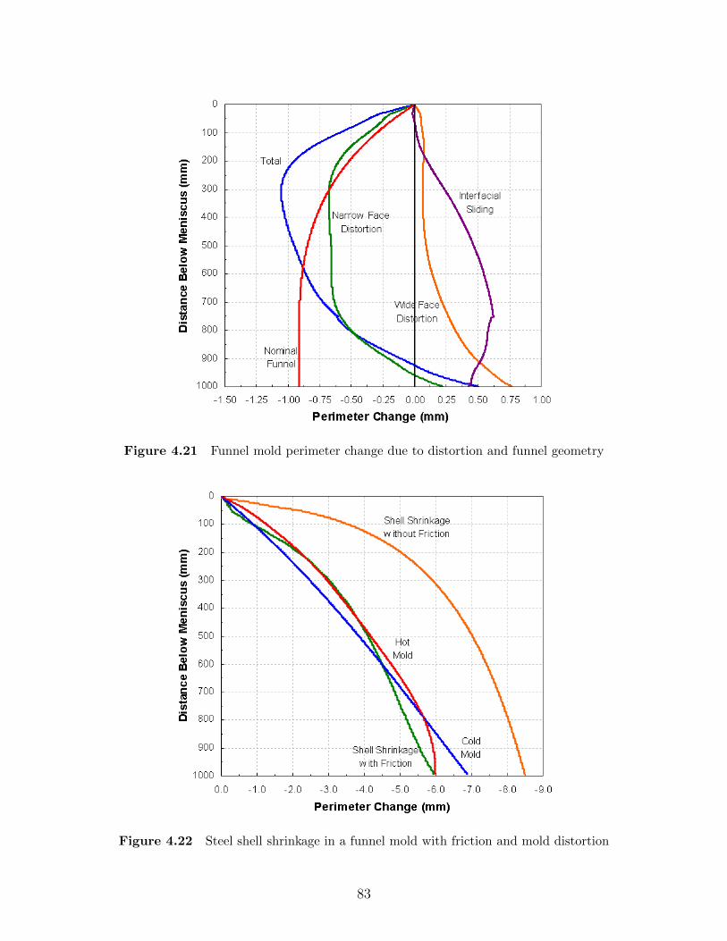
Figure 4.21 Funnel mold perimeter change due to distortion and funnel geometry

Figure 4.22 Steel shell shrinkage in a funnel mold with friction and mold distortion

83

range of operating conditions found in commercial practice.

4.6 Online Measurement of Mold Distortion and Taper

The instantaneous nf tapers were measured in real time during casting with inclinometers.

Each nf waterbox was instrumented with two inclinometers, one centered at 94 mm below the

top of the mold plate, and the other centered at 31 mm above the bottom of the mold plate,

as shown in Figure 4.25. The inclinometers give a nominal ±5 V signal for ±3◦ angle from

vertical, which is scaled to a ±10 V signal for ±6◦ angle based on the calibration certificates.

The signal from the inclinometers is filtered with a first-order low-pass filter to remove the

noise created by the mold oscillation.

The simulations of the mold presented in this section are compared with the inclinometer

measurements. The distorted nf shape is a combination of the distortion of the mold itself,

governed by its waterbox, and of the frictional contact with the wide face. The mold is

assembled and clamped together while at room temperature, and as the mold heats and

expands during startup, the friction between the mold faces resists some of the tendency

for the nf mold to deform. The orange “Sticking nf” curve in Figure 4.26 shows the shape

of the mold about 2 min after the start of mold filling, at a vcast = 3.5 m/min steady state.

This curve is calculated as the nominal taper plus Narrow Face Distortion plus Interfacial

Sliding from Section 4.5.6. The model predictions of mold orientation match the inclinometer

measurements to within 2′ at the top and to within 1′ at the bottom of the mold.

When the clamping forces are released for a strand-width change during casting, the

frictional forces disappear, and the nf mold takes on a different shape, shown by the blue

“Sliding nf” curves in Figures 4.26 and 4.27. This curve is calculated as the nominal taper

plus Narrow Face Distortion from Section 4.5.6. The model predictions of mold orientation

match the inclinometer measurements to less than 1′ for both the top and bottom of the

mold. The simulations show that the slope of the distorted NF mold in the middle of the

mold is in good agreement with the applied taper. The taper near the top and bottom of

the mold is substantially different than this nominal value, due to the important effect of

mold thermal distortion.

4.7 Conclusions

This chapter provides insight into the mechanical behavior of steel continuous-casting molds

during steady casting, based on a nonlinear d finite-element elastic stress analysis. The

84

Figure 4.23 Strand-mold gap in a funnel mold with friction and mold distortion

Figure 4.24 Funnel mold nf wear predictions and measurements

85

Figure 4.25 Funnel mold nf instrumented with inclinometers

model features realistic thermal boundary conditions based on plant measurements, complete

geometric details of the mold plates and waterboxes, tightened bolts and tie-rods, and realistic

contact with friction and ferrostatic pressure.

For beam-blank molds, the regions of of the hot face furthest from the water channel

become very hot, especially at the meniscus. These hot spots are found at the “shoulder,”

and are alleviated with smaller and/or more water channels in the region. The mold generally

bows outward, away from the steel, with a slight twisting motion. This distorted shape,

calculated in d, has been translated into a moving-slice d Lagrangian database for use

with the multiphysics model presented in Chapter 5.

Owing to the changes in water cooling around the mold bolts and near mold exit on

the wide face, combined with widely varying bolt stiffnesses, the wide face contorts into a

w shape in both the perimeter- and casting-directions. The predicted shape of the narrow

face was validated with inclinometers measurements; measuring taper with inclinometers is

a powerful tool for mold operation.

For both beam-blank molds and funnel molds, the narrow face distorts into a parabolic

arc a few millimeters deep. These behaviors are predictable and must be accommodated

when designing taper practices. The distortion of the narrow face in a funnel mold was

validated with inclinometer measurements from a plant trial, and match to within a few

arc-minutes.

The results of the funnel-mold distortion simulation were evaluated from an operational

perspective, considering the potential for several different practical problems:

1. Mold distortion has a significant effect on mold taper. The thermal distortion of each

of the mold pieces, the effect of the changing funnel geometry, and the interfacial

sliding of the wide and narrow faces all contribute to the effective taper seen by the

solidifying shell, each in a nonlinear fashion with distance down the mold. The thermal

86

0 1 2 3 4 5 6 7 8 9 10

Relative Position of Hot Face (mm)

0

100

200

300

400

500

600

700

800

900

1000

1100

Dis

tance

Bel

owT

op

of

Moldz

(mm

)

23.8′ Nom.

Measured: 35.8′

Sticking NF: 33.7′

Sliding NF: 39.6′

Measured: 20.5′

Sticking NF: 19.6′

Sliding NF: 33.7′

After Startup

Figure 4.26 Funnel mold nf shape and inclinometer measurements after startup

0 1 2 3 4 5 6 7 8 9 10

Relative Position of Hot Face (mm)

0

100

200

300

400

500

600

700

800

900

1000

1100

Dis

tance

Bel

owT

op

of

Moldz

(mm

)

18.0′ Nom.

Measured: 34′

Sliding NF: 33.2′

Measured: 6′

Sliding NF: 6.1′

After Width Change

Figure 4.27 Funnel mold nf shape and inclinometer measurements after width change

87

expansion of the wide face works against the applied taper and the effect of the funnel,

so calculations based only on room-temperature dimensions are insufficient.

2. To avoid shell buckling and cracks, the thermal distortion of the mold should be con-

sidered when designing taper practices.

3. The mold pieces are in strong contact just below meniscus and just above mold exit,

where temperatures are highest. The meniscus region could experience scratching

due to slag infiltration into a thin, 0.2 mm, interfacial gap. The submeniscus region

could experience the “crushing” phenomenon observed in previous work unless care

is taken to avoid excessive clamping forces.

4. Mold wear was estimated by superimposing the total effect of the thermal distortion

of the mold and a linear 1 %/m taper on previous calculations of the shell behavior.

Although this taper generally produces acceptable matching with the shell shrinkage,

the shell is predicted to wear against the mold just below the meniscus and near mold

exit. Plant measurements of mold wear are consistent with this prediction.

5. The mold bolts have no risk of either tensile failure or shearing failure at the mold-

waterbox interfaces, owing to the bolt holes being sufficiently oversized.

88

CHAPTER 5

Multiphysics Model of Continuous Casting1

5.1 Introduction

This chapter presents a multi-physics, multi-field, multi-domain model of the continuous

casting process that accounts for turbulent fluid flow, heat transfer, solidification, and

mechanical distortion. The multiphysics model is demonstrated for continuous casting in the

beam-blank mold presented in earlier chapters.

As the demand for better computer simulations of solidification processes increases,

there is a growing need to include the effects of fluid flow into thermo-mechanical analyses.

The multiphysics approach of simulating all three macroscale phenomena (i.e. fluid flow,

solidification heat transfer, and mechanical distortion) simultaneously has been demonstrated

in several previous works [5, 38, 51], but is very computationally demanding for realistic

problems. Major difficulties stem from the inherently different coordinate descriptions and

numerical techniques used in the separate models for these three fields. Fluid flow typically

is performed on structured Eulerian domains using steady-state control-volume methods

with iterative solution algorithms. Stress analysis typically is performed on unstructured

Lagrangian domains using transient finite-element methods with direct solvers. Many different

methods are used to treat heat transfer with moving solidification front(s) [101]. Further

difficulties arise from the complex geometries, which require large computational meshes.

The steel continuous casting process has been analyzed with two d multiphysics mod-

els [38, 51] that include fluid flow, deformation of the shell and mold, and a coupled shell-

mold interfacial gap. The melting of gallium was explored with these same phenomena [94].

Some researchers have decoupled the thermal-flow analysis from the deformation analy-

sis [17, 23, 61, 66, 75, 87], but doing so neglects the important effects of the deformation,

namely the behavior of the interface between the casting and the mold [92].

Alternatively, the fluid flow simulation can be decoupled from the deformation analysis

1Much of the work presented in this chapter has been published by the author [35, 39, 96] and colleagues.Beyond the content of these articles, this chapter contains an updated literature review and some details thatwere not included in the original publications. The modeling effort presented in this chapter is a collaborativeeffort between the author, S. Koric, who was responsible for the solidifying strand simulations with his new“enhanced latent heat” technique [41], and R. Liu, who was responsible for the fluid-flow simulations. Theauthor was responsible for the mold simulations, and interfacing between the three models.

89

of the shell if the shape of the liquid pool can be estimated a priori, such as in continuous

casting of steel and aluminium, or cryolite electrolysis. Simulations of such processes can

readily output the “superheat flux” that delivers heat to the liquid side of the solidification

front. A recent simulation [41] demonstrated that this superheat flux can be incorporated

into a transient simulation of heat transfer in the solid and mushy region by enhancing the

latent heat in the mush, without explicitly tracking the solidification front.

5.2 Solidifying Shell Model

The earliest work that analyzed the deformation of solidifying bodies considered a semi-

infinite plate, using various semi-analytical techniques [76, 99, 103]. However, the complexity

of solidification-deformation problems generally is too difficult for closed-form analytical

solutions, and computational methods, typically the finite-element method, quickly became

the usual method of analysis [7, 26, 44, 104]. Cylindrical geometries were able to be analyzed

with numerical approaches [7, 115]. The solidifying metal has been treated as everything from

elastic [99, 104] to elastic–perfect-plastic [7, 103] to elastic-viscoplastic [40, 44, 45, 52, 76, 114,

115, 118]. The literature has a few examples of other approaches for solidification-deformation

problems that seem to have fallen out of use, such as the boundary-element method [29] and

internal-variable inelasticity [15]. Solidifying bodies usually are modeled with a Lagrangian

description of motion, but the Arbitrary Eulerian–Lagrangian (ale) technique has been

implemented as well [79].

The solidifying steel shell is modeled as a transverse Lagrangian slice that moves down

through the mold at the casting speed. Many continuum mechanics texts [4, 16] may

serve as general references for this finite-deformation model. The strains mostly are small

during solidification deformation problems, but the capability to handle arbitrary rotations

is necessary to model some parts of the shell in a continuous casting mold. The mechanical

behavior of the strand is governed by the quasi-static conservation of momentum,

0 = ∇ · � + b, (5.1)

where � is the cauchy stress tensor and b is the body force density vector, which is

neglected in this work. Following the multiplicative decomposition of the deformation

gradient [46, 49], the total rate-of-deformation tensor D additively decomposes into an

inelastic, thermodynamically-irreversible part Die and a thermoelastic, thermodynamically-

reversible Dte part as

D = Dte + Die. (5.2)

90

Linearized thermo-hypoelasticity provides part of the constitutive relationship between the

stress and the thermoelastic rate of deformation as

Dte = �T +CCC−1 :4� (5.3)

where � is the thermal expansion tensor, CCC is the fourth-rank elastic stiffness tensor, and

4� = � + �W −W� (5.4)

is the jaumann stress rate, where W is the spin tensor, i.e., the anti-symmetric part of the

velocity gradient. The inelastic rate-of-deformation tensor requires an additional constitutive

relationship Die = Die(�, T, . . .).

For the macroscale simulation presented in this chapter, the solidifying steel is assumed to

be an isotropic polycrystalline material, so the elastic stiffness tensor is defined by hooke’s

law, Equation (4.5), and the thermal expansion tensor is � = αEI, where

3αE = −1

ρ

∂ρ

∂T(5.5)

is the isotropic “differential” coefficient of thermal expansion calculated from the change of

mass density ρ with temperature T . Inelastic effects are described with a bodner [8, 9]-type

“unified” function, assumed to follow “J2 plasticity” with isotropic hardening. The inelastic

rate-of-deformation tensor then is described by the prandtl–reuss equations,

Die = ˙εie 3

2

�′

σ, (5.6)

where σ =√

32�′ : �′ is the von mises effective stress and

�′ = � − pI (5.7)

is the deviatoric part of the cauchy stress tensor, where p = 13

tr(�) is the pressure.

The effective inelastic strain rate ˙εie, a scalar, is calculated as

˙εie = fγC

(σ − f1ε

ie∣∣εie∣∣f2−1

)f3

exp

(−QT

), (5.8)

where

Q = 44 465 (5.9)

f1 = 130.5− 5.128× 10−3T (5.10)

f2 = −0.6289 + 1.114× 10−3T (5.11)

f3 = 8.132− 1.54× 10−3T (5.12)

fγC = 46 550 + 71 400CC + 12 000C2C, (5.13)

91

with T and Q in K, and carbon composition CC in wt. %, for austenite. Equation (5.8) was

fit [43] to high-temperature tensile [107] and creep [93] test data. In the temperature range

of austenite, f3 evaluates to between 6.5 and 5.5, which indicates climb-assisted glide as the

underlying mechanism of inelastic behavior [36]. The activation energy Q = 370 kJ/mol is

larger than the self-diffusion activation energy of iron (284 kJ/mol), which likely is a conse-

quence of the fitting. The form of Equation (5.8) allows an algorithmic approximation [52]

of kinematic hardening, where the effective stress σ and inelastic strain rate ˙εie are signed

according to the largest direct stress component; this approach demonstrates reasonable

agreement [52] with the limit cycle of some cyclic test data [93] at 1300 ◦C. For δ-ferrite, the

effective inelastic strain rate is calculated [118] as

˙εie = 0.1

∣∣∣∣∣σ

fδC(T

300

)−5.52(1 + 1000εie)m

∣∣∣∣∣

n

, (5.14)

where

m = 0.3495− 0.941 56× 10−6T (5.15)

1/n = −0.061 66 + 0.1617× 10−3T (5.16)

fδC = 13.678× 103C−0.556× 10−3

C . (5.17)

This form of a constitutive law is not a standard fit, so the underlying mechanism cannot be

exposed by the value of the stress exponent. However, Equation (5.14) does give stresses in

the δ-ferrite about an order of magnitude smaller than the austenite. The biggest challenge

to good constitutive models here is the lack of experimental data at elevated temperatures.

In both Equations (5.8) and (5.14), the von mises effective stress σ is expected in MPa and

the effective inelastic strain rate ˙εie is in 1/s. The δ-ferrite function, Equation (5.14), is used

when the δ-ferrite volume fraction is greater than 10%. The effective inelastic strain is the

integral of the effective inelastic strain rate, i.e.,

εie =

∫ t

0

˙εie dτ, (5.18)

which is used as the inelastic state variable in this work. If a material point is above a

coherency temperature, then εie = 0.

In the mechanical model of the solidifying shell, the liquid and mush are modeled as

isotropic perfect-plastic solids with a low yield strength, i.e.,

˙εfl =σ − σY

3µ∆t, (5.19)

92

where σY = 0.01 MPa is the strength of the “liquid” and µ is the shear modulus of the liquid;

µ∆t acts like a dynamic shear viscosity of the liquid. The inelastic strain in the liquid ˙εfl

is called “fluid strain,” and does not affect the behavior of the solid, i.e, εfl 6= εie, though

it serves the same purpose as inelastic strain in the liquid. The strength is chosen small

enough to effectively eliminate stresses in the liquid-mushy zones, but large enough to avoid

computational difficulties.

The thermal behavior of the solidifying shell is governed by the conservation of energy,

written for a spatial description of motion as

ρ

(∂h

∂t+ (vmaterial − vmesh) · ∇h

)= ∇ · (K · ∇T ), (5.20)

assuming no sources and negligible viscous dissipation, where h is the temperature-dependent

specific enthalpy including the latent heat of solidification, T is temperature, and K is the

temperature-dependent thermal conductivity tensor. In the Lagrangian description of motion

used to model the shell behavior, the computational mesh moves at the same velocity as

the material, i.e., vmesh = vmaterial. Consistent with the above assumption of isotropy, the

thermal conductivity tensor reduces to K = kI. The boundary conditions on Equation (5.20)

are insulated, i.e., −k∇T = 0, because of symmetry or because the liquid-only region of the

domain, discussed later, is assumed to be well-mixed, or a prescribed heat flux in the form

of a convection condition, i.e., −k∇T = h (T − T0), where h is the heat-transfer coefficient

and T0 is the sink temperature.

The governing equations are solved incrementally using the finite-element method in

abaqus [1], using an implicit stepwise-coupled algorithm [25] for the time integration of the

governing equations. The constitutive laws are integrated by solving a system of ordinary

differential equations at each material point using the backward-euler method with bounded

newton steps [42] in the user subroutine umat. Each time step occurs as two sub-steps: the

thermal field is integrated at fixed configuration, and then the mechanical field is integrated

at adiabatic conditions, driven by the increment of thermal strain. Global newton iterations

continue until tolerances for both the thermal and mechanical equation systems are satisfied

before proceeding to the next time step.

Temperature and phase-dependent enthalpy [28], thermal conductivity [28], thermal

expansion [28], and elastic modulus [60] were calculated for 0.071 % wt. C plain carbon steel

with solidus and liquidus temperatures of Tsol = 1471.9 ◦C and Tliq = 1518.7 ◦C. The volume

fractions of the liquid, delta, and austenite phases, shown in Figure 5.1, are calculated

according to a linearized phase diagram [105]. Other simulation conditions are listed in

Table 4.4.

93

The Lagrangian shell-model domain given in Figure 5.2, was discretized with 32 874 nodes

and 63 466 degrees of freedom, and required 12 409 time steps for the complete 45 s simulation

down the mold length. The domain is a thin “stripe” of the strand section adjacent to the

mold wall that is thick enough to allow twice the expected shell thickness at mold exit to

solidify, while avoiding calculation of the liquid behavior away from the mold wall. More

importantly, the enclosed space which represents the internal liquid cavity is able to shrink

to properly model liquid feeding of the real continuous casting process.

This d transient model also comprises a d solution at steady state. The slice begins

at the top of the liquid steel pool, where the uniform initial conditions are the pouring

temperature, Tinit, zero displacement, zero strain, and zero stress. The d assumption is valid

for the thermal analysis, owing to negligible axial conduction because of the large peclet

number Pe = vcast`mold/α, where vcast is the casting speed, `mold is the mold length, and α

is the thermal thermal diffusivity [21]. The appropriate two-dimensional mechanical state is

that of generalized plane strain with negligible out-of-plane bending, which has been shown

capable of reproducing the complete d stress state [40].

5.3 Fluid Flow Model

A d fluid flow model of the pool of molten steel solves for the time-averaged velocity and

pressure distributions in an Eulerian domain. The fluid velocities v are calculated for a

divergence-free velocity field,

∇ · v = 0, (5.21)

using the momentum balance with advection terms,

ρ

(∂v

∂t+ v · ∇v

)= ∇ · � + b, (5.22)

for an incompressible Newtonian fluid, which has constitutive relationship for the cauchy

stress tensor of

� = Cµk2

ε

(∇v +∇v>

)− pI, (5.23)

where p is pressure, k is the specific turbulent kinetic energy, ε is the specific turbulent

dissipation rate, and Cµ = 0.09 is a constant. The k and ε fields are found by solving the two

additional transport equations given by the standard k-ε turbulence model [48]. Buoyancy

phenomena are negligible relative to the flow inertia, as indicated by Gr/Re2 ≈ 10−3, where

Gr is the grashoff number and Re is the reynolds number. The temperature field is

calculated from the energy equation, Equation (5.20), with no mesh velocity vmesh = 0 for

94

Figure 5.1 Phase fractions for 0.071 % wt. C plain carbon steel

Figure 5.2 Shell model domain with thermo-mechanical boundary conditions

95

Condition Value Unit

Mass density 6800 kg/m3

Kinematic shear viscosity 0.006 m2/sInlet velocity 1.854 m/sInlet turbulent intensity 200 %Inlet kinetic energy 0.464 J/kgInlet dissipation rate 2.077 J/(kg · s)Inlet diameter 25.5 mmInlet area 256 mm2

Top surface area 0.032 m2

Outflow area 0.0215 m2

Casting speed 0.0148 m/s

Table 5.1 Flow simulation conditions

the Eulerian description of motion. The velocity and temperature fields thus are decoupled,

so the flow affects the temperature but the temperature does not affect the flow. The

governing equations are discretized with the finite-volume method, and solved using the

simple method and first-order upwinding for the advective terms in the governing equation.

The flow problem is solved with the commercial software fluent [3], to give the pressure,

velocity, and temperature fields at each cell in the computational domain, and the heat flux

at the domain boundary surfaces.

The domain for the flow model is bounded by the symmetry planes of the mold and

the position of the solidification front, defined as the liquidus temperature, extracted from

the solidifying shell model described in Section 5.2. The molten steel enters the liquid

pool through two pour funnels, indicated in Figure A.6, with a Reynolds number of about

54× 103; this feature is modeled as a prescribed v , k, and ε over an appropriate circular

inlet on the top surface of the domain. The “standard” wall functions are used to model the

steep velocity gradients near the solid-liquid interface. Symmetry planes are treated with the

appropriate symmetry boundary conditions of no normal velocity and no tangential traction.

The motion of the strand is modeled as the solid-liquid interface velocity being downward at

the casting speed. To account for the solidification of the shell, the solid-liquid interface is

given appropriate mass and momentum sinks [78] with a user-defined function in fluent.

Figure 5.3 shows the velocity and temperature distributions on the center plane and top

plane, 10 mm below the free surface, calculated with the d thermo-fluid flow simulation of

606 720 hexahedral cells. Table 5.1 summarizes the conditions of this simulation.

96

Figure 5.3 Velocity and temperature distributions in the molten steel pool

97

5.4 Mold Model

In this work, a d finite-element model of one symmetric fourth of the beam-blank mold

assembly was constructed to capture the effects of mold distortion and variable mold surface

temperature on the solidifying steel shell. The beam-blank mold is not symmetric across

the casting radius, but this assumption was made for simplifying the demonstration of the

multiphysics process model. The model mold and water box geometries include the curvature

and applied taper of the hot faces, water channels, and bolt holes as described in Section A.2.

The mesh consists of 263 879 nodes and 1 077 166 tetrahedron, wedge, and hexahedron

elements. The governing equations and model description are presented in Sections 2.2 and

4.2. The hot face of the mold is applied a heat flux which is extracted from the surface of

the solidifying shell model described in Section 5.2. Inelastic effects are neglected because of

the negligible influence on the steady operating behavior of the mold [63]. Contact between

the two mold pieces and two backing plates was enforced manually by iteratively applying

constraint equations on contacting nodes. The mold bolts and tie rods were simulated using

linear truss elements and were appropriately pre-stressed, as described in Section 4.3.

The calculated temperature and distortion results are presented in Figure 4.5 In addition

to providing insight into thermo-mechanical behavior of the mold, as discussed in Chapters 2

and 4, this model provides temperature and displacement boundary conditions for the model

of the solidifying shell model discussed in Section 5.2.

5.5 Fluid/Shell Interface Treatment

Results from the fluid flow model of the liquid domain affect the solidifying shell model by

the heat flux crossing the boundary, which represents the solidification front, or liquidus

temperature. This “superheat flux” can be incorporated into a fixed-grid simulation of heat

transfer phenomena in the mushy and solid regions by enhancing the latent heat [41] of

the solidifying material. This method enables accurate decoupling of complex heat-transfer

phenomena into separate simulations of the fluid flow region and the mushy and solid region.

The energy boundary condition at a liquid-solid interface is the stefan condition [21]:

− qsolid · ninterface + qliquid · ninterface = ρsolidhfvinterface · ninterface, (5.24)

In the model of the solidifying steel shell, the liquid region is taken as isothermal so no heat

flows, i.e., qliquid = 0. However, the qliquid from the flow simulation discussed in Section 5.3,

which is not zero, is modeled as an increase to the latent heat such that the stefan condition

98

in the shell model becomes

− qsolid · ninterface = ρsolid (hf + ∆hf) vinterface · ninterface, (5.25)

where the “enhanced latent heat” ∆hf is calculated as

∆hf =

∣∣∣∣qliquid · ninterface

ρsolidvinterface · ninterface

∣∣∣∣ . (5.26)

The latent heat enhancement is added to the nominal latent heat and enthalpy in Equa-

tion (5.20) with the umatht user subroutine in abaqus. Because of the limitations of

abaqus,2 the normal interface speed vinterface · ninterface is estimated from the local cooling

rate T and temperature gradient ∇T at every time and material point near the solidification

front as

vinterface · ninterface =T

‖∇T‖2

=∆T

∆t

1

‖∇T‖2

. (5.27)

Equation (5.27) produces excessive and fluctuating latent heat values when the temperature

increments ∆T are driven to be very small by the global newton iterative procedure,

particularly at early solidification times and when the superheat flux is large, such as near

the pouring cup in the beam-blank mold. This issue is circumvented in this work by using

an analytical solution for the interface speed when the total latent heat exceeds 40 times the

nominal latent heat. The analytical solution [21] is that of the “solid-control” solidification

solution with superheat. The solidification constant φ is determined by solving

cp,s (Tliquidus − Tsurface) = φ exp(φ2)

erf(φ)√π

(hf +

qliquid · ninterface

ρsolidφ√αsolid/t

)(5.28)

The normal interface speed then is calculated as

vinterface · ninterface = φ

√αsolid

t. (5.29)

This approach gives an accurate and smooth estimate of the interface speed, and performs well

in both one- and two-dimensional solidification problems [41]. The additional heat delivered

to the solidification front by the fluid causes the shell to solidify more slowly than without

this superheat. Most most shell models in the literature use the technique of enhancing the

thermal conductivity of the liquid [59] to account for the advection of the liquid, which causes

the shell to solidify faster.

2The umatht subroutine provides only information local to an integration point, including T and ∇T .Better methods exist to calculate the interface speed that involve the temperature field across an element,but they cannot be implemented in abaqus.

99

The superheat flux qliquid · ninterface that is calculated at the boundaries of the d steady

Eulerian fluid flow model is converted to a function of space and time for the Lagrangian shell

model. Each point on the perimeter p(x, y) around the surface of the flow model is chosen

as the liquidus isotherm. These surface coordinates and the calculated superheat flux are

stored in arrays of Nperimeter points around the perimeter for each of the Nz layers of nodes

below the meniscus. At a given time t in the shell model, the corresponding distance below

the meniscus is z = vcastt. The array of coordinates is searched to find the indicies i and i+ 1,

where 1 ≤ i ≤ Nperimeter, and j and j+ 1, where 1 ≤ j ≤ Nz, which bound the material point

in the Lagrangian shell model. The corresponding superheat fluxes at array coordinates (i, j),

(i+ 1, j), (i, j + 1), and (i+ 1, j + 1) then are bilinearly interpolated. The interpolation

uses the standard basis functions for a quadrilateral finite element, using local coordinates

ξ = 2 (p− pi) / (pi+1 − pi)− 1 in the perimeter direction and η = 2 (z − zj) / (zj+1 − zj)− 1

in the axial direction, where p is the x-coordinate for points on the wide face and is the

y-coordinate for points on the narrow face.

Figure 5.4 shows a d view of the superheat flux distribution on the shell interface

calculated from the turbulent flow model. The fluid flow causes uneven distribution of

superheat fluxes that are greatest midway down the inner shoulder, and least in the flange and

center of the wide face. These variations in turn cause local shell thinning and temperature

changes, which affect the thermal stress behavior.

The enhancement to the latent heat described above is valid strictly at a sharp liquid-solid

interface. The multiphysics model in this work uses a phase-averaged energy equation [20],

so this dissonance must be reconciled. The heat flowing into a patch of the sharp interface

with area A at position x∗ from the liquid can be rewritten as a volumetric quantity as

∫

A

qliquid(x∗) · ninterface dA =

∫

V

qliquid(x) · ninterfaceδ(x − x∗) dV, (5.30)

using a property of the dirac delta [20]. Let φliquid be an “indicator function” that is unity

in the liquid and zero otherwise; the gradient of this function is ∇φliquid = δ(x − x∗) ninterface.

The volumetric heat flux then is∫

V

qliquid(x) · ninterfaceδ(x − x∗) dV =

∫

V

qliquid(x) · ∇φliquid dV. (5.31)

The multiphysics model uses volume-fraction fields f that partition unity instead of sharp

indicator functions; the gradients of these functions are related by

limxliquid−xsolid→0

∇fliquid · (xliquid − xsolid) = ∇φliquid · ninterface, (5.32)

100

Figure 5.4 Superheat flux distribution on the liquid-solid interface

101

where xliquid and xsolid are the positions of the liquidus (fliquid = 1) and of the solidus

(fliquid = 0) isopleths. The finite mushy zone size introduces a length scale to the enhanced

latent heat method, which must be small relative to the other major thermal length scale,

the thickness of the solidified shell, for a consistent thermal model. For the first few moments

after initial solidification in the continuous casting process, these two length scales are nearly

equal, but eventually the length of the mushy zone is about an order of magnitude smaller

than the shell thickness. For both the ultra-low-carbon grade used in the funnel mold and

the low-peritectic grade used in the beam-blank mold in this work, `mush/`shell ≈ 0.1 by mold

exit. That the volumetric heat flux is proportional to ∇fliquid indicates that the enhancement

to the latent heat is applied spatially closer to the liquidus isopleth for steel, and for other

materials with an effective partition coefficient less than unity, which yields an approximately

consistent approach with extracting the superheat flux from the flow model at the location

of the liquidus.

The effect of the ferrostatic pressure in the liquid pool is treated in the shell model as a

linearly-increasing distributed load that pushes the solidifying steel shell towards the mold,

as described by Equation (4.18). This boundary condition is implemented with the abaqus

user subroutine dload.

5.6 Shell/Mold Interface Treatment

Two-way thermo-mechanical coupling between the shell and mold is needed because the

stress analysis depends on temperature via the thermal strains and material properties, and

the heat conducted between the mold and steel strand depends strongly on the distance

between the separated surfaces calculated from the mechanical solution. Heat transfer across

the interfacial gap between the shell and the mold wall surfaces is defined with a resistor

model that depends on the thickness of gap calculated by the mechanical model. The total

heat transfer qgap occurs along two parallel paths, one due to radiation, hrad, and one due to

conduction, hcond, as

qgap = (hrad + hcond) (Tshell − Tmold) . (5.33)

The radiation heat transfer coefficient is calculated across the transparent liquid portion of

the mold slag layer as

hrad =σSB

1εshell

+ 1εmold

− 1

(T 2

shell + T 2mold

)(Tshell + Tmold) , (5.34)

where σSB = 56.704 nW/(m2 ·K4) is the stefan–boltzmann constant, εshell = εmold = 0.8

are the emissivities of the shell and the mold surfaces, and Tshell and Tmold are the absolute

102

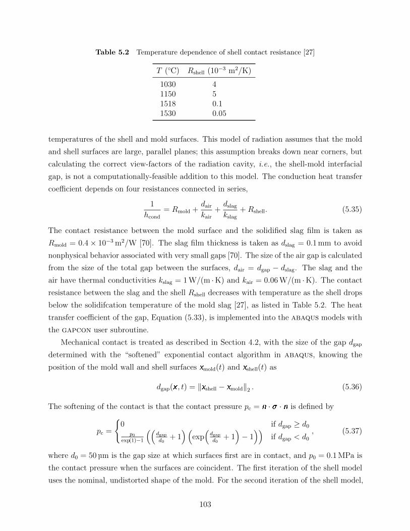
Table 5.2 Temperature dependence of shell contact resistance [27]

T (◦C) Rshell (10−3 m2/K)

1030 41150 51518 0.11530 0.05

temperatures of the shell and mold surfaces. This model of radiation assumes that the mold

and shell surfaces are large, parallel planes; this assumption breaks down near corners, but

calculating the correct view-factors of the radiation cavity, i.e., the shell-mold interfacial

gap, is not a computationally-feasible addition to this model. The conduction heat transfer

coefficient depends on four resistances connected in series,

1

hcond

= Rmold +dair

kair

+dslag

kslag

+Rshell. (5.35)

The contact resistance between the mold surface and the solidified slag film is taken as

Rmold = 0.4× 10−3 m2/W [70]. The slag film thickness is taken as dslag = 0.1 mm to avoid

nonphysical behavior associated with very small gaps [70]. The size of the air gap is calculated

from the size of the total gap between the surfaces, dair = dgap − dslag. The slag and the

air have thermal conductivities kslag = 1 W/(m ·K) and kair = 0.06 W/(m ·K). The contact

resistance between the slag and the shell Rshell decreases with temperature as the shell drops

below the solidifcation temperature of the mold slag [27], as listed in Table 5.2. The heat

transfer coefficient of the gap, Equation (5.33), is implemented into the abaqus models with

the gapcon user subroutine.

Mechanical contact is treated as described in Section 4.2, with the size of the gap dgap

determined with the “softened” exponential contact algorithm in abaqus, knowing the

position of the mold wall and shell surfaces xmold(t) and xshell(t) as

dgap(x , t) = ‖xshell − xmold‖2 . (5.36)

The softening of the contact is that the contact pressure pc = n · � · n is defined by

pc =

{0 if dgap ≥ d0

p0

exp(1)−1

((dgap

d0+ 1)(

exp(dgap

d0+ 1)− 1))

if dgap < d0

, (5.37)

where d0 = 50 µm is the gap size at which surfaces first are in contact, and p0 = 0.1 MPa is

the contact pressure when the surfaces are coincident. The first iteration of the shell model

uses the nominal, undistorted shape of the mold. For the second iteration of the shell model,

103

Figure 5.5 Solidifying slice for validation problem

the results of the d mold distortion model were post-processed to create a database of

surface temperature Tmold(p, t) and surface position xmold(p, t) for points on the transverse

perimeter of the hot face p and distance down the mold z. This database was created, using

the same procedure described in Section 5.5, to turn the d fields into transient d fields

for the Lagrangian shell model as a function of time below the meniscus, t = z/vcast. A

time-varying displacement is applied to each point on the hot face to re-create the distorted

shape of the mold that the Lagrangian shell domain would encounter as it moves through

the mold, using the abaqus user subroutine disp.

5.7 Validation of the Numerical Models

The thermo-mechanical solidification model used in this work is validated with the semi-

analytical solution of thermal stresses in an unconstrained solidifying plate [103]. A one-

dimensional model of this test casting can produce the complete d stress and strain state

if the condition of generalized plane strain is imposed in both the width (y) and length (z)

directions [52].

The domain adopted for this problem moves with the strand in a Lagrangian frame of

reference as shown in Figure 5.5. The domain consists of a thin slice through the plate thick-

ness using d 4-node generalized plane strain elements, in the axial z direction, implemented

in abaqus. The second generalized plane strain condition was imposed in the y-direction,

parallel to the surface, by coupling the y-displacements of all nodes along the bottom edge

of the slice domain. A fixed temperature is imposed at the left boundary, and all other

boundaries are insulated.

The material in this problem has elastic–perfect-plastic constitutive behavior. The

104

yield stress drops linearly with temperature from 20 MPa at 1000 ◦C to zero at the solidus

temperature 1494.4 ◦C, which was approximated by σY = 0.03 MPa at the solidus temperature.

A narrow mushy region, 0.1 ◦C, is used to approximate the single melting temperature assumed

in the analytical solution. Table 5.3 summarizes the conditions of the validation problem.

Condition Value Unit

Thermal conductivity 33 W ·K/mSpecific heat capacity 661 J/(kg ·K)Young’s modulus in solid 40 GPaYoung’s modulus in liquid 14 GPaPoisson’s ratio 0.3 –Coefficient of linear expansion 20 (µm/m)/KMass density 7500 kg/m3

Liquidus temperature 1494.45 ◦CFusion temperature (analytical) 1494.4 ◦CSolidus temperature 1494.35 ◦CInitial temperature, no superheat 1495 ◦CInitial temperature, with superheat 1545 ◦CLatent heat of fusion 272 kJ/kgSurface temperature 1000 ◦C

Table 5.3 Conditions for solidifying steel in the validation problem

Figures 5.6 and 5.7 show the temperature and the stress distribution across the solidifying

shell at two different solidification times. The mesh with 0.3 mm-square elements accurately

matches the analytical solutions for both fields. For free-shrinking metal slabs, the surface

is in compression and the solidification front is in tension because the surrounding material

constrains the slab to remain planar and resists the tendency of the material to shrink [103].

More details about this model validation can be found elsewhere [30, 42, 52] including

comparisons with other less-efficient integration methods and a convergence study.

The method for modeling superheat by enhancing latent heat is also tested on the same

slice domain and compared with a d analytical solution for conduction with phase change [21].

The superheat flux is best calculated with simultaneous modeling of fluid flow; instead the

initial temperature is increased by 50 ◦C to provide a superheat flux driven by the temperature

difference between Tinit and Tliq, assuming stagnant liquid. To test the enhanced latent heat

method, the validation problem was first executed with the large superheat, and the heat flux

at the moving solidification front during post-processing. The validation problem then was

executed again with a small superheat and the enhanced latent heat method implemented

in the user subroutine umatht, with this extracted superheat flux. Figure 5.8 shows the

105

Figure 5.6 Validation problem temperature evaluation without superheat

Figure 5.7 Validation problem stress evaluation without superheat

106

Figure 5.8 Validation problem shell growth with enhanced latent heat technique

analytical and numerical solidification front positions, with and without the 50 ◦C superheat;

the “Numerical with Superheat” points in the plot shows that the enhanced latent heat

method can accurately solve this solidification problem using the post-processed superheat

flux.

5.8 Multiphysics Model of Beam-Blank Casting

The multiphysics model presented in this chapter was used to find the fluid-flow, tem-

perature, stress, and deformation in a complex-shaped beam blank caster under realistic

continuous casting conditions. Figure 5.9 is a flow chart of the solution strategy for the

thermo-mechanical-fluid flow model of steel continuous casting. First, the thermo-mechanical

model of the solidifying shell is simulated assuming a uniform superheat distribution driven

by the temperature difference between Tinit and Tliq, and artificially increasing thermal con-

ductivity in the liquid region seven-fold. The first shell model uses a simplified thermal model

of the mold, like what is presented in Chapter 3, with the nominal, undistorted shape of

the mold hot face. The heat flux from the shell surface provide the boundary conditions for

the thermo-mechanical model of the mold, which in turn supplies the next run of the shell

model with mold temperature and thermal distortion boundary conditions. The position of

107

the solidification front in the shell model defines an approximate shape of the liquid pool for

the fluid flow model, which is used to calculate the superheat flux distribution for the next

iteration of the shell model. Finally, an improved thermo-mechanical model of solidifying

shell is re-run which includes the effects of the superheat distribution and mold distortion,

and completes the first iteration of the multiphysics model. Because the shell profile from

the improved thermo-mechanical model has little effect on superheat results in the liquid

pool, a single multiphysics iteration is sufficient to predict the shell growth accurately.

The shoulder region of the beam-blank mold has a convex shape which converges the

heat flow and increases local temperature, opposite to behavior at the corners. Figures 5.10

and 5.11 show the calculated gaps at the shoulder and flange. A gap in the middle shoulder

is caused by outward bending of the shell due to contact pressure from the mold onto the

middle of the flange. Heat extraction from the shoulder is therefore retarded as shown in

Figure 5.10, yielding a thinner shell with higher temperature. The shell pulls away from the

both corners of the flange, shown in Figure 5.11, but by differing amounts; the “flange tip”

corner is well-cooled by the narrow face, but the “flange corner” corner is consistently the

hottest part of the surface of the shell. Figures 5.12 and 5.13 gives the temperature and

gap size of several key locations around the perimeter of the hot face. The maximum and

minimum principal stress contours at 457 mm below meniscus are given in Figure 5.14, which

show the expected compressive shell behavior at the “cold” surface and tensile stress in the

hot interior near the solidification front, similar to the model validation from Figure 5.7. The

tendency for the surface to be in compression and the solidification front to be in tension is

mainly a consequence of the constraint provided by the surrounding material, as mentioned

in Section 5.7, though other effects like the increasing strength with decreasing temperature

and changes to the heat removal because of the coupled gap behavior or mold geometry

affect the behavior as well. Maximum stress and strain is found in the shoulder area, which

is not a surprise since the thinner shell in this region caused by gap formation leads to stress

concentration. Longitudinal cracks and breakouts are often found in this same shoulder

region, as revealed by plant observations [35].

108

Figure 5.9 Flowchart for multiphysics solution strategy

109

Figure 5.10 Calculated temperatures and gaps at the shoulder of the beam-blank mold

Figure 5.11 Calculated temperatures and gaps at the flange of the beam-blank mold

110

Figure 5.12 Calculated temperature histories of several points on the surface of thebeam-blank strand

Figure 5.13 Calculated gap-size histories of several points on the surface of thebeam-blank strand

111

(a) Maximum in-plane principal stress(b) Minimum in-plane principal stress

Figure 5.14 Stresses in the solidifying shell at 457 mm below meniscus, in Pa

112

The shell thickness, defined as 90% fraction-liquid, predicted by a thermo-mechanical–only

model (the first iteration) and the multiphysics model of the soldifiying strand are compared

with measurements around the perimeter of a breakout shell [35] in Figure 5.15. The initial

thermo-mechanical model with a uniform superheat distribution can only roughly match the

shell thickness variations. Shell thickness variations at the corners and shoulder due to air gap

formations were captured with to the interfacial heat transfer model. The variable field in the

multiphysics model correctly calculates the accelerated shell growth in the middle of the web,

where the liquid is the coldest, and the retarded shell growth at the corner, where the liquid

is the hottest. The shell is about 4 mm thicker in the middle of the flange and 2 mm thinner

at the shoulder with the multiphysics model than what it is in the thermo-mechanical–only

model. The improved multiphysics model that includes the fluid flow effects matches the

shell thickness measurement around the entire perimeter much more accurately. This finding

illustrates the improved accuracy that is possible by including the effects of fluid flow into a

thermal stress analysis of solidifying shell.

5.9 Conclusions

The model developed in this chapter enables accurate uncoupling of complicated multiphysics

phenomena in continuous casting into separate simulations of the fluid flow region, the

mushy zone and solid steel shell region, and the mold. Spatially and temporally non-

uniform superheat fluxes, produced by turbulent fluid flow and mixing in the liquid pool, are

calculated from the results of a finite-volume fluid flow model. A new latent-heat method

is applied to link these results into a coupled thermo-mechanical finite-element model of

the solidifying shell. The realistic effect of mold thermal distortion is incorporated through

a second database and boundary condition at the shell-mold interface. The model first is

validated with available analytical solutions of thermal stress, temperature, and shell growth.

The model then is applied to simulate solidification in a one-quarter transverse section of

a commercial beam blank caster with complex geometry, temperature dependent material

properties, and realistic operating conditions. The results compare very well with in-plant

measurements of the thickness of the solidifying shell.

This method illustrates an effective approach towards accurate multiphysics modeling

of commercial processes. By exploiting unique features of the continuous casting of steel,

individual models can be coupled together in an efficient, accurate, and robust way to achieve

realistic predictions of metal solidification on the continuum scale. The key is the careful

choice of the boundaries between modeling domains, and their treatment in both interface

113

models, such that convergence can be achieved in as little as one iteration on the macroscale.

The most intimately-coupled phenomena, i.e., the coupled thermal and mechanical behavior

of the shell-mold interfacial gap, are modeled in the same domain and model.

Realistic prediction of shell shape, temperature, and shrinkage is just the first step in

predicting the formation of defects such as porosity, segregation, and cracks, microstructure,

and final properties. Much further work remains to incorporate further models of these

additional phenomena into useful modeling systems, tailored for a given process like casting

or welding.

114

Figure 5.15 Calculated and measured shell thickness around the perimeter ofbeam-blank section

115

CHAPTER 6

Conclusions and Future Work

This work has explored some aspects of the continuous casting of steel with numerical models.

The main contribution of this work is to develop a multiphysics, macroscale model of the

process that simulates the coupled effects of turbulent flow and heat transport in the molten

steel pool, the elastic-viscoplastic thermal shrinkage and solidification heat transfer in the

solid steel shell, and the thermal distortion of the mold. This complete model of the process

is possible because of the largely “one-way coupling” between the fields and domains, and

appropriate techniques for interfacing between the models.

The multiphysics modeling process begins with a model of heat transfer in the solidifying

shell. This first shell model must be able to match the plant-measured thermocouple tem-

peratures and cooling water temperature change before proceeding to the remaining steps in

the multiphysics procedure. This first shell model is post-processed for the heat flux from

the shell into the mold, and for the position of the solidification front. These data are used

to drive a elastic thermo-mechanical simulation of the mold distortion and to define the

solid-liquid interface in a turbulent thermal-flow model of the liquid steel pool. The mold

distortion calculation is post-processed for the temperature and distorted shape of the hot

face of the mold, and the fluid flow simulation is post-processed for the heat flux entering

the solid shell at the solidification front. The realistic mold hot face and the superheat flux

distribution then are fed into a separate elastic-viscoplastic thermo-mechanical model of the

solidifying shell, which requires special boundary conditions that represent the physics of

their respective interfaces, and careful translation to change from Eulerian to Lagrangian

descriptions of the fields. The multiphysics modeling approach allows each main phenomenon

to be modeled accurately in a “natural” setting for each set of physics, e.g., the fluid flow is

simulated with an Eulerian fixed-grid approach.

To avoid the full coupling of the first shell model of the solidifying shell with the mold, the

thermal effect of the mold is approximated with a one-dimensional analytical model, which

results in a convection condition that represents all of the physics of the mold. The parameters

in this simple analytical model related to the mold geometry first are calibrated so that this

reduced-order model of mold heat transfer is able to match the temperature predictions of

a small finite-element model of the exact mold geometry. Only one calibration is necessary

116

per mold geometry, as the method was demonstrated in Chapter 3 to be insensitive to the

boundary conditions on the calibration domain. This fast and simple model of mold heat

transfer is a useful tool by itself, but also provides an accurate representation of the mold

in larger models of the continuous casting process, such as a model of the shell deformation,

where computational effort is better spent on the physics of interest of the main model.

Only three-dimensional models with good geometric fidelity to the actual mold, such as

the models presented in Chapters 2 and 4, can reveal the variations in mold temperature

on the hot face and throughout the mold, particularly around the cooling channels of the

mold. These variations, though small relative to the other temperatures on the hot face,

can have negative consequences on the cast product, up to and including breakouts. Good

geometric fidelity also is necessary when predicting the distorted shape of the mold, and

the model of the mold distortion must contain the waterboxes and bolts that support and

contact the molds. The simulated shape of the narrow face mold agrees very well with

measurements from inclinometers on an in-service mold. The applied taper on the molds

has been calculated, and measured, to change significantly because of the thermal expansion

of the mold: for example, the local taper, including the effect of mold distortion, near mold

exit of a funnel mold was about three times smaller than the nominal taper that was applied

to the mold. Quantitative knowledge of the shape of the mold at operating temperatures is

vital to properly design the taper practice and avoid defects in the cast steel.

Moreover, the uneven distribution of superheated liquid in the molten steel pool affects

the behavior of the solidifying steel. This work demonstrated a technique for calculating

this distribution of temperature in a flow model, and modifying the solidification boundary

condition in a thermo-mechanical simulation of the shell to simulate its effect. A multiphysics

model of the solidifying shell, including the effects of this uneven distribution of superheat

and the distorted shape of the mold, is presented in Chapter 5, for a beam-blank mold. This

particular geometry showcases the need for such a model because of the many two- and

three-dimensional physical phenomena that cannot be captured with the previous approach

to modeling the continuous casting process. For example, the shell growth is accelerated by

about 10% in the middle of the web region of the cast section because of the much larger

distance to the stream of the hot steel, and the multiphysics model is capable of matching this

measured observation, while the traditional thermo-mechanical model is not. The prediction

of the multiphysics model matches measurements of the varying thickness of a breakout shell

all the way around the perimeter of the mold.

The multiphysics modeling approach demonstrated in this work has redefined the state

of the art of continuous casting process modeling. Creating a model of a process neces-

117

sarily involves making assumptions about the behavior of the process to create a feasible

computational model, and for most of continuous casting these assumptions are reasonable.

Sometimes these assumptions prevent the model from calculating correct behavior, such as

remelting of the shell under a submerged molten steel jet, or with the complicated geometry

of a beam blank mold. However, these problems are no longer an issue with the modeling

framework developed in this work. This comprehensive macroscale view of the process has

been demonstrated to accurately match many different measurements from the plant, and can

be extended in future work to include microscale effects and to investigate defect formation

from a more fundamental perspective. For example, conditions of a typical segment of the

strand calculated in the multiphysics model can be used as boundary conditions on microscale

studies of defect formation.

118

APPENDIX A

Mold Geometry

Continuous casting molds are shaped to cast:

• billets and blooms, which are square sections with rounded corners

• rounds, which are circular sections

• rectangular slabs, ranging from 50 mm–90 mm “thin” slabs to 250 mm “thick” slabs

• “beam-blanks” which are a dogbone section, and

• strips, in the range of a few millimeters thick, though this variant of continuous

casting is still under development.

The tendency of the steel industry over the last few years has been to move to near-net-shape

castings, such as thin-slab and beam-blank, for among other reasons to reduce rolling costs.

Some thin-slab casters include a gentle funnel cut into the hot face of the molds to allow

space for the sen to fit between the mold plates. This work covers a thin-slab funnel mold

and a beam-blank mold, and this appendix outlines the geometry of these mold sections.

A.1 Funnel Mold

The funnel mold and its waterbox considered in this work are shown in Figures A.1 through

A.5. One symmetric fourth of the mold is considered for computational efficiency, though the

waterbox is not symmetrical. Other asymmetric effects, like variations in bolt tightening or

mold alignment, and the mold geometry changes to accommodate the the mold-level sensor

on one side, are expected to be small. This mold has no coating layers. Except for the top

row, each bolt is instrumented with a thermocouple set 20 mm from the hot face.

The funnel opening on the wide face decreases from 136.8 mm at mold top to 106 mm

at mold exit. The funnel has an “inner flat” region in the center, which transitions to an

“outer flat” region near the narrow faces by means of two tangent circles of equal radius but

opposite curvature, as shown in Figure A.1. Further detail of funnel mold geometry is given

in Chapter 2 of Reference 30. The wide face water channels are 5 mm wide by 15 mm deep,

cut with a ball-end mill, and set 20 mm from the hot face with 10 mm spacing in banks of

18, as shown in Figure A.2. The inlets and outlets of the water channels curve away from

119

Figure A.1 Funnel mold wf mold geometry

Figure A.2 Funnel mold wf waterchannel geometry

the hot face to meet the waterbox. Each

wide face has a rectangular array of 81 bolts

spaced 125 mm apart in the casting direction and

212.5 mm apart in the horizontal direction. The

cooling passages next to each bolt hole are a pair

of 10 mm-diameter tubes. There are 18 channels

and 2 tubes between bolt columns. Three water

channels are cut into one wider channel, centered

at 323.75 mm from the centerline, for about half

the length of the mold, to accommodate a mold

level sensor. The wide face waterbox, shown in

Figure A.3, is built from 20 mm-, 30 mm-, and

50 mm-thick plates, and includes large 587.5 mm-

by-650 mm cavities to accommodate an electro-

magnetic flow control system.

The narrow face mold plate is 72 mm thick

and its waterbox is 110 mm thick with a 50 mm

bore for the water flow, as shown in Figure A.4.

Each narrow face copper plate is cooled by four

14 mm diameter cylindrical water tubes. The hot face of the narrow face is curved slightly

concave towards the molten steel to ensure that any bulking of the strand during soft reduction

below the mold is outward. Each narrow face is attached with a column of bolts with 134 mm

spacing to a waterbox that is suspended by large hooks on two support cylinders. These two

support cylinders are dynamically positioned to adjust mold width and taper.

120

Figure A.3 Funnel mold wf mold and waterbox geometry

121

Figure A.4 Funnel mold nf mold and waterbox geometry

The finite-element mesh used in the funnel-mold simulations is shown in Figure A.5.

As listed in Table A.1, this multi-part mesh consists of 1.36 million nodes and 5.15 million

elements. The mold and waterbox were modeled with very good geometric accuracy, including

the water channels and bolt holes. The mold bolts are approximated as truss elements, as

discussed in Section 4.3. Further details are given in the body of this document.

Table A.1 Funnel mold simulation mesh details

Part Nodes Elements

Wide Face Mold Plate 855 235 4 223 072Wide Face Waterbox 185 534 190 457Wide Face Bolts 90 45Tie Rods 4 2Narrow Face Mold Plate 233 931 495 566Narrow Face Waterbox 83 269 239 604Narrow Face Bolts 16 8

Total 1 358 079 5 148 754

122

Figure A.5 Funnel mold and waterbox mesh

123

A.2 Beam-Blank Mold

The beam-blank mold and its waterbox considered in this work are shown in Figures A.6

through A.8. Two versions of the beam-blank mold geometry were considered: one with

half-symmetry and one with quarter-symmetry, though the waterbox is not symmetrical.

Other asymmetric effects, like variations in bolt tightening or mold alignment, are expected

to be small. This mold has no coating layers.

The beam-blank profile shown in Figure A.6 is 576 mm wide, and has a 436 mm-wide

flange and a 93 mm-thick web. The mold has various ball-end–milled water channels around

the perimeter of the bottoms of the flanges, and several large cooling tubes around the web

and tops of the flanges. The cooling tubes all have internal “restrictor rods” to increase the

speed of the cooling water. A slice through the middle of the web is shown in Figure A.7,

which identifies the mold thicknesses at various points down the length of the mold. Figure A.7

also shows the locations of several thermocouples that were instrumented in this mold for

the model validation discussed in Section 2.3.

The quarter-symmetry finite-element mesh used in the beam-blank-mold simulations is

shown in Figure A.8. This multi-part mesh consists of 264 thousand nodes and 1.08 million

elements. The mold and waterbox were modeled with very good geometric accuracy, including

the casting radius of the hot face, the water channels, and the bolt holes. The mold bolts

are approximated as truss elements, as discussed in Section 4.3. Further details are given in

the body of this document.

124

Figure A.6 Beam-blank mold geometry, top view

Figure A.7 Beam-blank mold geometry, slice through wf centerline

125

Figure A.8 Beam-blank mold and waterbox mesh

126

APPENDIX B

The Eigenvalues and Eigenvectors of a 3× 3 Matrix1

Eigenvalue problems permeate engineering and science, so the ability to calculate efficiently

both the eigenvalues and eigenvectors of a matrix is important. Calculating the principal

stresses and strains, and their principal directions, is an example of an eigen-problem related

to the deformation analysis work in Chapter 5. Three-dimensional problems take a special

place in this class of problems because of the nature of the physical world. This appendix

presents a method to calculate efficiently and accurately the eigenvalues and eigenvectors

of an arbitrary 3 × 3 real matrix. An explicit, algebraic expression for the eigenvectors is

presented.

B.1 Introduction

Consider an arbitrary 3× 3 matrix A with real-valued components Aij,

[A]

=

A11 A12 A13

A21 A22 A23

A31 A32 A33

. (B.1)

The statement of the (right) eigen-problem is to find the scalar-vector pair λ, x such that

the action of the matrix A upon the vector x is the same as scaling the vector by λ, i.e.,

Ax = λx, (B.2)

and λ is called an eigenvalue and x is its associated eigenvector. Non-trivial solutions to

Equation (B.2), i.e., x 6= 0, are found by requiring that

0 = det(A− λI) , (B.3)

where det(·) is the matrix determinant operator and I is the identity matrix. Expanding

Equation (B.3) provides the characteristic equation of the matrix,

0 = −λ3 + I1λ2 − I2λ+ I3, (B.4)

1The content of this chapter was created entirely by the author, independent of other coauthors, includinghis advisor. This work will soon be submitted for publication.

127

where the principal invariants I1, I2, and I3 are

I1 =A11 + A22 + A33, (B.5a)

I2 =A22A33 + A33A11 + A11A22 − A23A32 − A31A13 − A12A21, (B.5b)

I3 =A11A22A33 + A23A31A12 + A32A13A21 − A11A23A32 − A22A31A13 − A33A12A21. (B.5c)

Re-casting the characteristic equation, Equation (B.4), in terms of the deviatoric principal

invariants of A simplifies the problem at hand. The deviatoric part A′ of the matrix A is

A′ = A− pI, (B.6)

where, borrowing the language from the stress tensors, the quantity

p =1

3I1 (B.7)

is the “pressure.” The principal invariants of A′ are expressible in terms of the principal

invariants of A as

J1 = 0 (B.8a)

J2 = 3p2 − I2 (B.8b)

J3 = I3 + p(2p2 − I2

). (B.8c)

A few arithmetical operations are saved,2 however, by computing the deviatoric invariants

directly from the components of the matrix A, i.e.,

J1 =0, (B.9a)

J2 =1

6

((A22 − A33)2 + (A33 − A11)2 + (A11 − A22)2)

+ A23A32 + A31A13 + A12A21,(B.9b)

J3 = (A11 − p) (A22 − p) (A33 − p) + A23A31A12 + A32A13A21

− (A11 − p)A23A32 − (A22 − p)A31A13 − (A33 − p)A12A21.(B.9c)

The substitution λ = `+ p into the characteristic equation of A, Equation (B.4), gives

0 = −`3 + J2`+ J3, (B.10)

2As a side note, J2 can be computed with one less addition, multiplication and division than Equa-tion (B.9b) using

J2 = (A11 − p)2 − (A22 − p) (A33 − p) +A23A32 +A31A13 +A12A21,

or with cyclic permutations of the A11, A22, and A33 terms. However, these expressions are more prone toproblems with round-off errors than Equation (B.9b), to the point where J2 can be negative for symmetricmatrices. Robustness should be favored over the small increase in execution speed.

128

i.e., the characteristic equation of A′. Without the quadratic term, Equation (B.10) is in

some sense easier to solve than Equation (B.4) for finding the eignevalues, as discussed in

Section B.2.

B.2 Calculating the Eigenvalues

The characteristic equation of a 3× 3 matrix is a cubic equation, whose solution dates back

to the sixteenth-century Italian mathematicians del ferro, tartaglia, and cardano [12].

The closed-form algebraic solution for the eigenvalues λ provided by the cubic formula

necessarily involves complex arithmetic, which is inconvenient when all eigenvalues are real.

The eigenvalues of A are computed as

λ1 = p+ 2a (B.11a)

λ2 = p− a− j√

3b (B.11b)

λ3 = p− a+ j√

3b, (B.11c)

where

2a = c+ d (B.12a)

2b = c− d (B.12b)

c3 = K3 +√K2

3 −K32 (B.12c)

d3 = K3 −√K2

3 −K32 (B.12d)

3K2 = J2 (B.12e)

2K3 = J3, (B.12f)

and j =√−1 is the imaginary unit. An alternative approach, due to viete [100], exploits

the trigonometric identity

cos(3θ) = 4 cos3(θ)− 3 cos(θ) , (B.13)

which, with the substitution u = cos(θ), gives the cubic equation

0 = −u3 +3

4u+

1

4cos(3θ) . (B.14)

Now, let u = m`, so that Equation (B.14) is written as

0 = −`3 +3

4

1

m2`+

1

4

1

m3cos(3θ) , (B.15)

129

which is identical to the deviatoric characteristic equation, Equation (B.10), if J2 = 3/ (4m2)

and J3 = cos(3θ) / (4m3). Thus 1/m = 2√K2 and the angle θ is calculated by

θ =1

3arccos(k) , (B.16)

where k = K3/K3/22 . The angle θ is known as the lode angle in some mechanics applications,

and is an invariant quantity. The roots of Equation (B.14) are u = cos(θ), u = cos(θ − 2π/3),

and u = cos(θ + 2π/3), which allows the eigenvalues of A to be determined as

λ1 = p+ 2√K2 cos(θ) (B.17a)

λ2 = p+ 2√K2 cos(θ − 2π/3) (B.17b)

λ3 = p+ 2√K2 cos(θ + 2π/3) . (B.17c)

smith [90] evidently introduced engineers to the trigonometric approach for the eigenvalues

of a 3× 3 matrix, but avoided discussing the numerical issues that arise in the approach.

Equation (B.16) identifies that A has real eigenvalues when −1 ≤ k ≤ +1, or K23 ≤ K3

2 .

The case of J2 < 0 is not considered here. Examining Equations (B.17) reveals that A has

one distinct real eigenvalue λ = p only when K2 = 0, regardless of the behavior of k. The

matrix A has two distinct real eigenvalues when θ = nπ/3 for any integer n, which is possible

only when k = +1, or θ = 0, and when k = −1, or θ = π/3. The characteristic equation has

a polynomial discriminant of zero when k = ±1, which corresponds to K32 = K2

3 . Otherwise,

the eigenvalues are real and distinct, or are real and a complex-conjugate pair3.

If K2 6= 0, then Equation (B.17) gives the natural scaling for the eigenvalues as

Λi =λi − p2√K2

, (B.18)

where i = 1, 2, 3, and −1 ≤ Λi ≤ +1 when the eigenvalues are real. In terms of these scaled

eigenvalues, the polynomial to solve is

0 = −4Λ3 + 3Λ+ k, (B.19)

which is no easier to solve than the deviatoric characteristic equation, Equation (B.10), but

it does have advantageous properties when moving to a computer, namely that for real

eigenvalues the equation evaluates to values between −1 and +1. Indeed, introducing the

scaled matrix

D =1

2√K2

A′ (B.20)

3The case of J2 < 0 produces eigenvalues that are real and a complex-conjugate pair, but involves morecomplex arithmetic.

130

alleviates some of the numerical difficulties of the eigenvalue problem. Note that for the

matrix D, the invariants are J2 = 34

and J3 = 14k, where k is calculated for the matrix A as

described above; calculating k from the scaled matrix is less subject to numerical cancellation

errors.

Using the trigonometric identities 2 cos(x± 2π/3) = − cos(x)∓√

3 sin(x), the eigenvalues

are written4 as

Λ1 = cos(θ) (B.21a)

2Λ2 = − cos(θ) +√

3 sin(θ) (B.21b)

2Λ3 = − cos(θ)−√

3 sin(θ) , (B.21c)

which saves one evaluation of a trigonometric function. The arccosine function extended over

the entire real line is

arccos(x) =

π − j arcosh(−x) if x ≤ −1

arccos(x) if −1 ≤ x ≤ +1

j arcosh(x) if +1 ≤ x

, (B.22)

and using the identities sin(x+ jy) = sin(x) cosh(y) + j cos(x) sinh(y) and cos(x+ jy) =

cos(x) cosh(y)− j sin(x) sinh(y), for k ≤ −1, the eigenvalues are

2Λ1 = cosh(θ′)− j√

3 sinh(θ′) (B.23a)

2Λ2 = cosh(θ′) + j√

3 sinh(θ′) (B.23b)

Λ3 = − cosh(θ′) , (B.23c)

with θ′ = −13

arcosh(−k), and for −1 ≤ k ≤ +1, the eigenvalues are

Λ1 = cos(θ′) (B.24a)

2Λ2 = − cos(θ′) +√

3 sin(θ′) (B.24b)

2Λ3 = − cos(θ′)−√

3 sin(θ′) , (B.24c)

with θ′ = 13

arccos(k), and for +1 ≤ k, the eigenvalues are

Λ1 = cosh(θ′) (B.25a)

2Λ2 = − cosh(θ′) + j√

3 sinh(θ′) (B.25b)

2Λ3 = − cosh(θ′)− j√

3 sinh(θ′) . (B.25c)

with θ′ = 13

arcosh(k). Figure B.1 shows a plot of Equations (B.23), (B.24), and (B.25). Note

that Figure B.1 reveals that λ1 ≥ λ2 ≥ λ3 always holds, so no effort need be expended on

sorting the computed eigenvalues.

4Equation (B.21) shows that evidently, a =√K2 cos(θ) and b = j

√K2 sin(θ) in the cubic formula,

Equation (B.11).

131

−3.0 −2.5 −2.0 −1.5 −1.0 −0.5 0.0 0.5 1.0 1.5 2.0 2.5 3.0

(J3/2) /√J2/3

3

−1.25

−1.00

−0.75

−0.50

−0.25

0.00

0.25

0.50

0.75

1.00

1.25

λ− p2√J2/3

Re(λ1) = Re(λ2)

Im(λ1)

Im(λ2)

λ3

λ1

λ2

λ3

λ1

Re(λ2) = Re(λ3)

Im(λ2)

Im(λ3)

Figure B.1 The eigenvalues of a 3× 3 matrix

Sufficiently far away from the cases of repeated eigenvalues, i.e, k = ±1, Equations (B.23),

(B.24), and (B.25) are adequate for use in computer implementation [90]. However, algorithms

should be designed around the difficult ranges of input. Consider now the case of all real

eigenvalues; as pointed out by simo and hughes [88, p. 244], the arccosine function is ill-

conditioned near the cases of repeated eigenvalues, and exploiting the trigonometric identity

arccos(x) =

arctan(√

1x2 − 1

)if x > 0

π2

if x = 0

π − arctan(√

1x2 − 1

)if x < 0

(B.26)

somewhat helps to alleviate the issue. scherzinger and dohrmann [85] demonstrated that

as |k| → 1, the eigenvalues computed from the trigonometric functions are accurate to about√εmach, where εmach is machine epsilon. scherzinger and dohrmann [85] then proposed

a method to find the eigenvalues and eigenvectors at the same time, which first finds the

“most distinct” eigenvalue, i.e., λ1 if k > 0 and λ3 if k < 0, transforms the matrix to a basis

where the eigenvector corresponding to the “most distinct” eigenvalue is one of the basis

vectors, and then solves accurately the quadratic equation for the other eigenvalues in the

transformed basis. Their method demonstrates accuracy on the order of machine precision,

but at the cost of larger execution time than other non-iterative methods for solving the

eigenproblem.

132

As far as the author has been able to determine, the accuracy of the scherzinger and

dohrmann [85] approach is paralleled only by well-conditioned iterative algorithms,5 though

these come at the cost of algorithmic overhead. The best alternative that the author could

produce is documented below.

Consider solving the scaled characteristic equation, Equation (B.19), using newton

iterations. Initial iteration values are found by first expanding Equation (B.19) about Λ0 to

second order,

− (12Λ0)Λ2 +(12Λ2

0 + 3)Λ+

(−4Λ3

0 + k)

= 0, (B.27)

and then taking Λ0 as −1, −1/2, 0, +1/2, and +1, to create several approximations of the

cubic equation,

0 = −12Λ2 − 15Λ− 4− k (B.28a)

0 = −6Λ2 − 6Λ− 1/2− k (B.28b)

0 = −3Λ− k (B.28c)

0 = 6Λ2 − 6Λ+ 1/2− k (B.28d)

0 = 12Λ2 − 15Λ+ 4− k. (B.28e)

The approximations are used in their appropriate ranges, broken around values of k that

give good approximations to the original cubic, as shown in Figure B.2, to provide initial

iteration values for the scaled eigenvalues,

0Λ1 =

12

(1 +

√23

(1 + k))

if k < −1/2

58

(1 +

√1675

(1 + k)− 115

)if −1/2 ≤ k

(B.29a)

0Λ2 =

12

(1−

√23

(1 + k))

if k < −2/3

−k/3 if −2/3 ≤ k ≤ +2/3

−12

(1−

√23

(1− k))

if +2/3 < k

(B.29b)

0Λ3 =

−5

8

(1 +

√1675

(1− k)− 115

)if k ≤ +1/2

−12

(1 +

√23

(1− k))

if +1/2 < k. (B.29c)

Equations (B.29) are written to avoid the usual cancellation problem with the quadratic

formula, but still suffer from cancellation under the radical. This cancellation under the

radical is the limit to high accuracy in this approach.

The newton method update is

i+1Λ = iΛ+ δΛ, (B.30)

5For example, DSYEV in the LAPACK library.

133

−1.00 −0.75 −0.50 −0.25 0.00 0.25 0.50 0.75 1.00(λ− p

)/(2√J2/3

)−1.00

−0.75

−0.50

−0.25

0.00

0.25

0.50

0.75

1.00

J3/2√J2/3

3

λ1

λ2

λ3

Figure B.2 Second-order approximations of the scaled cubic equation

where the standard correction is

δΛ = − f(iΛ)

f ′(iΛ). (B.31)

The function f , the scaled cubic equation, admits the factorization

f(Λ) = − (2Λ+ 1)2 (Λ− 1)− (1− k) (B.32)

for use when k > 0, and the factorization

f(Λ) = − (2Λ− 1)2 (Λ+ 1) + (1 + k) (B.33)

for use when k < 0, to help control cancellation and round-off errors. The derivative of the

function is

f ′(Λ) = −3 (2Λ− 1) (2Λ+ 1) . (B.34)

The correction is decomposed into partial fractions as

δΛ = −1

6

((2Λ− k + 1

2Λ− 1

)+

k − 1

2Λ+ 1

)(B.35)

if k > 0, and as

δΛ = −1

6

((2Λ+

k − 1

2Λ+ 1

)− k + 1

2Λ− 1

)(B.36)

if k < 0, coded exactly as parenthesized, to help control cancellation and round-off errors.

134

The newton method for this problem, given initial values from Equations (B.29), con-

verges to better than 3εmach in five or less iterations away from the region of two distinct

eigenvalues. Curiously, this approach maintains accuracy of about 3εmach for three nearly

repeated eigenvalues. For matrices with nearly two distinct eigenvalues, the accuracy is no

better than√εmach. The following techniques were explored:

1. newton iterations, as described above,

2. deflating the cubic polynomial to a quadratic polynomial and solving analytically,

3. deflating the cubic polynomial to a quadratic polynomial and solving the eigenvalue

problem for the companion matrix,

4. newton iterations for multiple roots (δΛ = ff ′/((f ′)2 − ff ′′

)), for both the cubic

and the quadratic equations

5. maehly–newton iterations,

6. using kahan summation with the newton iterations, for both the cubic and the

quadratic equations.

B.3 Calculating the Eigenvectors

The eigenvector x associated with the eigenvalue λ is found by solving the equations

A11x1 + A12x2 + A13x3 = λx1 (B.37a)

A21x1 + A22x2 + A23x3 = λx2 (B.37b)

A31x1 + A32x2 + A33x3 = λx3. (B.37c)

However, explicitly trying to solve this system of equations yields only the zero vector. The

issue is that the system of equations is homogeneous, which allows as a solution either the

zero vector or an arbitrary scaling of some particular vector, i.e., the eigenvector. Since the

vector has some amount of arbitrariness, take x1 as unity and then solve for x2 and x3 as

x2 =− ((A33 − λ)A21 − A23A31)

(A33 − λ) (A22 − λ)− A23A32

(B.38a)

x2 =− ((A33 − λ)A31 − A32A21)

(A33 − λ) (A22 − λ)− A23A32

. (B.38b)

135

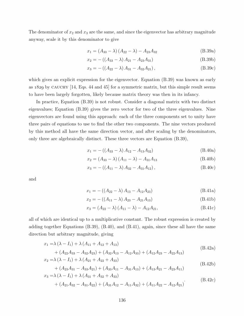
The denominator of x2 and x3 are the same, and since the eigenvector has arbitrary magnitude

anyway, scale it by this denominator to give

x1 = (A33 − λ) (A22 − λ)− A23A32 (B.39a)

x2 = − ((A33 − λ)A21 − A23A31) (B.39b)

x3 = − ((A22 − λ)A31 − A32A21) , (B.39c)

which gives an explicit expression for the eigenvector. Equation (B.39) was known as early

as by cauchy [14, Eqs. 44 and 45] for a symmetric matrix, but this simple result seems

to have been largely forgotten, likely because matrix theory was then in its infancy.

In practice, Equation (B.39) is not robust. Consider a diagonal matrix with two distinct

eigenvalues; Equation (B.39) gives the zero vector for two of the three eigenvalues. Nine

eigenvectors are found using this approach: each of the three components set to unity have

three pairs of equations to use to find the other two components. The nine vectors produced

by this method all have the same direction vector, and after scaling by the denominators,

only three are algebraically distinct. These three vectors are Equation (B.39),

x1 = − ((A33 − λ)A12 − A13A32) (B.40a)

x2 = (A33 − λ) (A11 − λ)− A31A13 (B.40b)

x3 = − ((A11 − λ)A32 − A31A12) , (B.40c)

and

x1 = − ((A22 − λ)A13 − A12A23) (B.41a)

x2 = − ((A11 − λ)A23 − A21A13) (B.41b)

x3 = (A22 − λ) (A11 − λ)− A12A21, (B.41c)

all of which are identical up to a multiplicative constant. The robust expression is created by

adding together Equations (B.39), (B.40), and (B.41), again, since these all have the same

direction but arbitrary magnitude, giving

x1 =λ (λ− I1) + λ (A11 + A12 + A13)

+ (A22A33 − A32A23) + (A32A13 − A12A33) + (A12A23 − A22A13)(B.42a)

x2 =λ (λ− I1) + λ (A21 + A22 + A33)

+ (A23A31 − A33A21) + (A33A11 − A31A13) + (A13A21 − A23A11)(B.42b)

x3 =λ (λ− I1) + λ (A31 + A32 + A33)

+ (A21A32 − A31A22) + (A31A12 − A11A32) + (A11A22 − A12A21). (B.42c)

136

The components of the eigenvectors given in Equations (B.39), (B.40), and (B.41) are

the determinants of the nine possible minors of the matrix A− λI. Also, evidently, Equa-

tion (B.42) is

x =(λ (λ− I1) I + λA + I3A

−1)

111

. (B.43)

Note that the inverse of A is not calculated explicitly; I3A−1 is the transpose of the adjugate

matrix of A. The cayley–hamilton theorem is used to rewrite the coefficient in Equa-

tion (B.43) as (λ (λ− I1) + I2) I+(λ− I1)A+A2, which then allows use of the characteristic

equation to rewrite the coefficient as (I3/λ) I + (λ− I1)A + A2. Since I1 = λ1 + λ2 + λ3

and I3 = λ1λ2λ3, the eigenvector associated with λ1 is

x1 = C1

111

, (B.44)

where

C1 = λ2λ3I − (λ2 + λ3)A + A2 (B.45)

and appropriately permuted for the other two eigenvectors. Equation (B.44) involves fewer

arithmetic operations than does Equation (B.43).

137

References

[1] ABAQUS 6.11 User Manuals. Dassault Simulia, 2011.

[2] D. Amsallem, M. J. Zahr, and C. Farhat. Nonlinear model order reduction based onlocal reduced-order bases. International Journal for Numerical Methods in Engineering,92(10):891–916, 2012.

[3] ANSYS Inc., Canonsburg, PA. ANSYS FLUENT 14 Theory Guide, 2011.

[4] R. J. Asaro and V. A. Lubarda. Mechanics of Solids and Materials. CambridgeUniversity Press, 2006.

[5] C. Bailey, P. Chow, M. Cross, Y. Fryer, and K. Pericleous. Multiphysics modelling ofthe metals casting process. Proceedings of the Royal Society of London A, 452:459–486,1996.

[6] J. Barbic and D. L. James. Real-time subspace integration for St. Venant–Kirchhoffdeformable models. ACM Transactions on Graphics, 24(3):982–990, 2005.

[7] H. G. Baumann and G. Schafer. Beitrag zur Berechnung der Kontraktion von Stahlwahrend seiner Erstarrung. Archiv fur das Eisenhuttenwesen, 41(12):1111–1115, 1970.

[8] S. R. Bodner and Y. Partom. A large deformation elastic-viscoplastic analysis of athick-walled spherical shell. Journal of Applied Mechanics, 39(3):751–757, 1972.

[9] S. R. Bodner and Y. Partom. Constitutive equations for elastic-viscoplastic strain-hardening materials. Journal of Applied Mechanics, 42(2):385–389, 1975.

[10] J. Burkardt, M. Gunzburger, and H.-C. Lee. POD and CVT-based reduced-order mod-eling of Navier–Stokes flows. Computer Methods in Applied Mechanics and Engineering,196(1-3):337–355, 2006.

[11] J. E. Camporredondo, A. H. Castillejos, F. A. Acosta, E. P. Gutierrez, and M. A.Herrera. Analysis of thin-slab casting by the compact-strip process: Part I. heatextraction and solidification. Metallurgical and Materials Transactions B, 35(3):541–560, 2004.

[12] H. Cardano. Artis Magnæ, Sive de Regulis Algebraicis Liber Unus. 1545.

[13] G. Carlsson, B. Brolund, and R. Nystrom. Measurement of mould distortion and mouldheat flux in industrial casters. Journees Siderurgiques ATS, 10, 1989.

[14] A.-L. Cauchy. Sur l’equation a l’aide de laquelle on determine les inegalites seculairesdes mouvements des planetes. In Exercices de mathematiques, volume 4, pages 140–160.De Bure freres, Paris, 1829. Reprinted in Œuvres Serie 2, vol. 9, pages 174–195.

138

[15] D. Celentano, S. Oller, and E. Onate. A coupled thermomechanical model for thesolidification of cast metals. International Journal of Solids and Structures, 33:647–673,1996.

[16] P. Chadwick. Continuum Mechanics: Concise Theory and Problems. George Allen &Unwin Ltd., London, 1976.

[17] A. Chatterjee and V. Prasad. A full 3-dimenisonal adaptive finite volume scheme fortransport and phase-change processes, part I: Formulation and validation. NumericalHeat Transfer A, 37:801–821, 2000.

[18] R. Chen, H. F. Shen, and B. C. Liu. Numerical simulation of fluid flow and solidificationin continuous slab casting mould based on inverse heat transfer calculation. Ironmakingand Steelmaking, 38(7):546–551, 2011.

[19] C. Chow, I. V. Samarasekera, B. N. Walker, and G. Lockhart. High speed continuouscasting of steel billets: Part 2: Mould heat transfer and mould design. Ironmaking andSteelmaking, 29(1):61–69, 2002.

[20] J. A. Dantzig and M. Rappaz. Solidification. Ecole Polytechnique Federale de LausannePress, 2009.

[21] J. A. Dantzig and C. L. Tucker. Modeling in Materials Processing. Cambridge UniversityPress, 2001.

[22] V. K. de Barcellos, C. R. F. Ferreira, C. A. dos Santos, and J. A. Spim. Analysis ofmetal mould heat transfer coefficients during continuous casting of steel. Ironmakingand Steelmaking, 37(1):47–56, 2010.

[23] C. del Borello and E. Lacoste. Numerical simulation of the liquid flow into a porousmedium with phase change: Application to metal composites processing. NumericalHeat Transfer A, 44:723–741, 2003.

[24] P. Feldmann and R. W. Freund. Efficient linear circuit analysis by Pade approximationvia the Lanczos process. IEEE Transactions on Computer-Aided Design of IntegratedCircuits and Systems, 14(5):639–649, 1995.

[25] C. A. Felippa and K. C. Park. Staggered transient analysis procedures for coupledmechanical systems: Formulation. Computer Methods in Applied Mechanics and Engi-neering, 24:61–111, 1980.

[26] A. Grill, K. Sorimachi, and J. K. Brimacombe. Heat flow, gap formation and break-outsin the continuous casting of steel slabs. Metallurgical Transactions B, 7(2):177–189,1976.

[27] H. N. Han, J.-E. Lee, T.-J. Yeo, Y. M. Won, K.-H. Kim, K. H. Oh, and J.-K. Yoon.A finite element model for 2-dimensional slice of cast strand. ISIJ International,39(5):445–454, 1999.

139

[28] K. Harste. Investigation of the Shrinkage and the Origin of Mechanical Tension duringthe Solidification and Successive Cooling of Cylindrical Bars of Fe-C Alloys. PhD thesis,Technical University of Clausthal, 1989.

[29] M. Heinlein, S. Mukherjee, and O. Richmond. A boundary element method analysis oftemperature fields and stresses during solidification. Acta Mechanica, 59(1–2):59–81,1986.

[30] L. C. Hibbeler. Thermo-mechanical behavior during steel continuous casting in funnelmolds. Master’s thesis, The University of Illinois at Urbana–Champaign, 2009.

[31] L. C. Hibbeler, M. M. Langeneckert, J. Iwasaki, I. Hwang, B. G. Thomas, and R. J.O’Malley. Calibration of thermal models of steel continuous casting molds. Iron andSteel Technology, 10(9):199–210, 2013.

[32] L. C. Hibbeler, B. G. Thomas, B. Santillana, A. Hamoen, and A. Kamperman. Lon-gitudinal face crack prediction with thermo-mechanical models of thin slabs in funnelmoulds. La Metallurgia Italiana, (2):1–10, 2009.

[33] L. C. Hibbeler, B. G. Thomas, R. C. Schimmel, and G. Abbel. The thermal distortionof a funnel mold. Metallurgical and Materials Transactions B, 43(5):1156–1172, 2012.

[34] L. C. Hibbeler, B. G. Thomas, R. C. Schimmel, and H. H. Visser. Simulation andonline measurement of narrow face mold distortion in thin slab casting. In Proceedingsof the 8th European Continuous Casting, 2014.

[35] L. C. Hibbeler, K. Xu, B. G. Thomas, S. Koric, and C. Spangler. Thermomechanicalmodeling of beam blank casting. Iron and Steel Technology, 6(7):60–73, 2009.

[36] W. F. Hosford. Mechanical Behavior of Materials. Cambridge University Press, 2005.

[37] Revised release on the IAPWS industrial formulation 1997 for the thermodynamicproperties of water and steam. Technical report, The International Association for theProperties of Water and Steam, 2007.

[38] J. E. Kelly, K. P. Michalek, T. G. OConnor, B. G. Thomas, and J. A. Dantzig. Initialdevelopment of thermal and stress fields in continuously cast steel billets. MetallurgicalTransactions A, 19(10):2589–2602, 1988.

[39] S. Koric, L. C. Hibbeler, R. Liu, and B. G. Thomas. Multiphysics model of metalsolidification on the continuum level. Numerical Heat Transfer B, 58(6):371–392, 2010.

[40] S. Koric, L. C. Hibbeler, and B. G. Thomas. Explicit coupled thermo-mechanical finiteelement model of steel solidification. International Journal of Numerical Methods inEngineering, 78:1–31, 2009.

[41] S. Koric and B. G. Thomas nad V. R. Voller. Enhanced latent heat method toincorporate superheat effects into fixed-grid multiphysics simulations. Numerical HeatTransfer B, 57:396–413, 2010.

140

[42] S. Koric and B. G. Thomas. Efficient thermo-mechanical model for solidificationprocesses. International Journal for Numerical Methods in Engineering, 66:1955–1989,2006.

[43] P. F. Kozlowski, B. G. Thomas, J. A. Azzi, and H. Wang. Simple constitutive equationsfor steel at high temperature. Metallurgical and Materials Transactions A, 23:903–918,1992.

[44] J. O. Kristiansson. Thermal stresses in the early stage of solidification of steel. Journalof Thermal Stresses, 5(3–4):315–330, 1982.

[45] J. O. Kristiansson. Thermomechanical behavior of the solidifying shell within continuouscasting billet molds- a numerical approach. Journal of Thermal Stresses, 7:209–226,1984.

[46] E. Kroner. Allgemeine Kontinuumstheorie der Versetzungen und Eigenspannungen.Archive for Rational Mechanics and Analysis, 4(1):273–334, 1959.

[47] M. M. Langeneckert. Influence of mold geometry on heat transfer, thermocoupleand mold temperatures in the continuous casting of steel slabs. Master’s thesis, TheUniversity of Illinois at Urbana–Champaign, 2001.

[48] B. E. Launder and D. B. Spalding. The numerical computation of turbulent flows.Computer Methods in Applied Mechanics and Engineering, 3:269–289, 1974.

[49] E. H. Lee. Elastic-plastic deformation at finite strain. Journal of Applied Mechanics,36(1):1–6, 1969.

[50] J.-E. Lee, H. N. Han, K. H. Oh, and J.-K. Yoon. A fully coupled analysis of fluidflow, heat transfer and stress in continuous round billet casting. ISIJ International,39(5):435–444, 1999.

[51] J.-E. Lee, T.-J. Yeo, K. H. Oh, J.-K. Yoon, and U.-S. Yoon. Prediction of cracks incontinuously cast steel beam blank through fully coupled analysis of fluid flow, heattransfer, and deformation behavior of a solidifying shell. Metallurgical and MaterialsTransactions A, 31(1):225–237, 2000.

[52] C. Li and B. G. Thomas. Thermomechanical finite-element model of shell behavior incontinuous casting of steel. Metallurgical and Materials Transactions B, 35(6):1151–1172, 2004.

[53] X. Liu and M. Zhu. Finite element analysis of thermal and mechanical behavior in aslab continuous casting mold. ISIJ International, 46(11):1652–1659, 2006.

[54] R. B. Mahapatra, J. K. Brimacombe, I. V. Samarasekera, N. Walker, E. A. Paterson,and J. D. Young. Mold behavior and its influence on quality in the continuous casting ofsteel slabs: Part I. Industrial trials, mold temperature measurements, and mathematicalmodeling. Metallurgical Transactions B, 22(6):861–874, 1991.

141

[55] X. Meng and M. Zhu. Thermal behavior of hot copper plates for slab continuous castingmold with high casting speed. ISIJ International, 49(9):1356–1361, 2009.

[56] Y. Meng and B. G. Thomas. Heat-transfer and solidification model of continuous slabcasting: CON1D. Metallurgical and Materials Transactions B, 34(5):685–705, 2003.

[57] Y. Meng and B. G. Thomas. Modeling transient slag-layer phenomena in the shell/moldgap in continuous casting of steel. Metallurgical and Materials Transactions B, 34(5):707–725, 2003.

[58] Y. Meng and B. G. Thomas. Simulation of microstructure and behavior of interfacialmold slag layers in continuous casting of steel. ISIJ International, 46(5):660–669, 2006.

[59] E. A. Mizikar. Mathematical heat transfer model for solidification of continuously caststeel slabs. Transactions of the Metallurgical Society of AIME, 239:1747–1753, 1967.

[60] H. Mizukami, K. Murakami, and Y. Miyashita. Elastic modulus of steels at hightemperature. Journal of the Iron and Steel Institute of Japan, 63(146):S–652, 1977.

[61] A. N. O. Moraga, D. C. Ramirez, M. J. Godoy, and P. D. Ticchione. Study of convectionnon-newtonian alloy solidification in moulds by the PSIMPLER/finite-volume method.Numerical Heat Transfer B, 57:936–953, 2010.

[62] H. Nam, H.-S. Park, and J. K. Yoon. Numerical analysis of fluid flow and heat transferin the funnel type mold of a thin slab caster. ISIJ International, 40(9):886–892, 2000.

[63] T. G. O’Connor and J. A. Dantzig. Modeling the thin-slab continuous-casting mold.Metallurgical and Materials Transactions B, 25(3):443–457, 1994.

[64] M. R. Ozgu. Mold and strand guide instrumentation for continuous slab casters. InProceedings of the 13th Process Technology Division Conference, 1995.

[65] M. R. Ozgu. Continuous caster instrumentation: State-of-the-art review. CanadianMetallurgical Quarterly, 35(3):199–223, 1996.

[66] R. Pardeshi, A. K. Singh, and P. Dutta. Modeling of solidification processes in rotaryelectromagnetic stirrer. Numerical Heat Transfer A, 55:42–57, 2009.

[67] H.-S. Park, H. Nam, and J. K. Yoon. Numerical analysis of fluid flow and heat transferin the parallel type mold of a thin slab caster. ISIJ International, 41(9):974–980, 2001.

[68] J. K. Park, I. V. Samarasekera, B. G. Thomas, and U. S. Yoon. Thermal and mechanicalbehavior of copper molds during thin-slab casting (I): Plant trial and mathematicalmodeling. Metallurgical and Materials Transactions B, 33(3):425–436, 2002.

[69] J. K. Park, I. V. Samarasekera, B. G. Thomas, and U. S. Yoon. Thermal and me-chanical behavior of copper molds during thin-slab casting (II): Mold crack formation.Metallurgical and Materials Transactions B, 33(3):437–449, 2002.

[70] J. K. Park, B. G. Thomas, and I. V. Samarasekera. Analysis of thermomechanical be-

142

haviour in billet casting with different mould corner radii. Ironmaking and Steelmaking,29(5):359–375, 2002.

[71] X. Peng, J. Zhou, and Y. Qin. Improvement of the temperature distribution incontinuous casting moulds through the rearrangement of the cooling water slots. Journalof Materials Processing Technology, 167(2–3):508–514, 2005.

[72] B. Petrus, K. Zheng, X. Zhou, B. G. Thomas, and J. Bentsman. Real-time, model-basedspray-cooling control system for steel continuous casting. Metallurgical and MaterialsTransactions B, 42(1):87–103, 2011.

[73] L. T. Pillage and R. A. Rohrer. Asymptotic waveform evaluation for timing analysis.IEEE Transactions on Computer-Aided Design of Integrated Circuits and Systems,9(4):352–366, 1990.

[74] C. A. M. Pinheiro, I. V. Samarasekera, J. K. Brimacombe, and B. N. Walker. Mouldheat transfer and continuously cast billet quality with mould flux lubrication: Part 1:Mould heat transfer. Ironmaking and Steelmaking, 27(1):37–54, 2000.

[75] M. Pokorny, C. Monroe, C. Beckermann, L. Bichler, and C. Ravindran. Prediction ofhot tear formation in magnesium alloy permanent mold casting. International Journalof Metalcasting, 2(4):41–53.

[76] O. Richmond and R. H. Tien. Theory of thermal stresses and air-gap formation duringthe early stages of solidification in a rectangular mold. Journal of the Mechanics andPhysics of Solids, 19(5):273–284, 1971.

[77] M. R. Ridolfi, B. G. Thomas, G. Li, and U. D. Foglia. The optimization of mold taperfor the Ilva-Dalmine round bloom caster. Revue de Metallurgie, 91(4):609–620, 1994.

[78] B. Rietow. Fluid velocity simulation and measurement in thin slab casting. Master’sthesis, The University of Illinois at Urbana–Champaign, 2007.

[79] J. M. Risso, A. E. Huespe, and A. Cardona. Thermal stress evaluation in the steel con-tinuous casting process. International Journal for Numerical Methods in Engineering,65(9):1355–1377, 2006.

[80] I. V. Samarasekera, D. L. Anderson, and J. K. Brimacombe. The thermal distortion ofcontinuous-casting billet molds. Metallurgical Transactions B, 13(1):91–104, 1982.

[81] I. V. Samarasekera and J. K. Brimacombe. The thermal field in continuous-castingmoulds. Canadian Metallurgical Quarterly, 18(3):251–266, 1979.

[82] I. V. Samarasekera and J. K. Brimacombe. Ironmaking and Steelmaking, 9:1–15, 1982.

[83] I. V. Samarasekera and J. K. Brimacombe. The influence of mold behavior on theproduction of continuously cast steel billets. Metallurgical Transactions B, 13(1):105–116, 1982.

143

[84] B. Santillana, L. C. Hibbeler, B. G. Thomas, A. Hamoen, A. Kamperman, andW. van der Knoop. Heat transfer in funnel-mould casting: Effect of plate thickness.ISIJ International, 48(10):1380–1388, 2008.

[85] W. M. Scherzinger and C. R Dohrmann. A robust algorithm for finding the eigenvaluesand eigenvectors of 3×3 symmetric matrices. Computer Methods in Applied Mechanicsand Engineering, 197:4007–4015, 2008.

[86] J. Sengupta, M. K. Trinh, D. Currey, and B. G. Thomas. Utilization of CON1Dat ArcelorMittal Dofasco’s no. 2 continuous caster for crater end determination. InProceedings of AISTech, 2009.

[87] M. R. Shamsi and S. K. Ajmani. Three dimensional turbulent fluid flow and heat transfermathematical model for the analysis of a continuous slab caster. ISIJ International,47:433–442, 2008.

[88] J. C. Simo and T. J. R. Hughes. Computational Inelasticity. Springer, New York, 1998.

[89] C. A. Sleicher and M. W. Rouse. A convenient correlation for heat transfer to constantand variable property fluids in turbulent pipe flow. International Journal of Heat andMass Transfer, 18(5):677–683, 1975.

[90] O. K. Smith. Eigenvalues of a symmetric 3× 3 matrix. Communications of the ACM,4(4):168, 1961.

[91] Steel Statistical Yearbook 2011. World Steel Association, 2011.

[92] D. Sun and S. V. Garimella. Numerical and experimental investigation of solidificationshrinkage. Numerical Heat Transfer B, 52:145–162, 2007.

[93] T. Suzuki, K. H. Tacke, K. Wunnenberg, and K. Schwerdtfeger. Creep propertiesof steel at continuous casting temperatures. Ironmaking and Steelmaking, 15:90–100,1988.

[94] A. Teskeredzic, I. Demirdzic, and S. Muzaferija. Numerical method for heat transfer,fluid flow, and stress analysis in phase-change problems. Numerical Heat Transfer B,42:437–459, 2002.

[95] B. G. Thomas, J. Jiang, and D. Lorento. Optimization of water channel design inbeam-blank molds. In Proceedings of the 5th European Continuous Casting Conference,pages 139–147, 2005.

[96] B. G. Thomas, S. Koric, L. C. Hibbeler, and R. Liu. Multiphysics model of continuouscasting of steel beam-blanks. In Proceedings of the 4th International Conference onModeling and Simulation of Metallurgical Processes in Steelmaking, 2011.

[97] B. G. Thomas, M. Langeneckert, L. Castella, M. Dziuba, G. di Gresia, and W. Balante.Optimisation of narrow face water slot design for Siderar slab casting mould. Ironmakingand Steelmaking, 30(3):235–239, 2003.

144

[98] B. G. Thomas, G. Li, A. Moitra, and D. Habing. Analysis of thermal and mechanicalbehavior of copper molds during continuous casting of steel slabs. Iron and Steelmaker,25(10):125–143, 1998.

[99] R. H. Tien and V. Koump. Thermal stresses during solidification on basis of elasticmodel. Journal of Applied Mechanics, 36(4):763–767, 1969.

[100] F. Viete. De Aequationum Recognitione et Emendatione. J. Laquehan, Paris, 1615.

[101] V. R. Voller. An overview of numerical methods for solving phase-change problems.Advances in Numerical Heat Transfer, 1(9):341–380, 1997.

[102] X. Wang, L. Tang, X. Zang, and M. Yao. Mold transient heat transfer behavior basedon measurement and inverse analysis of slab continuous casting. Journal of MaterialsProcessing Technology, 212(9):1811–1818, 2012.

[103] J. H. Weiner and B. A. Boley. Elasto-plastic thermal stresses in a solidifying body.Journal of the Mechanics and Physics of Solids, 11(3):145–154, 1963.

[104] J. R. Williams, R. W. Lewis, and K. Morgan. An elasto-viscoplastic thermal stressmodel with applications to the continuous casting of metals. International Journal forNumerical Methods in Engineering, 14(1):1–9, 1979.

[105] Y. M. Won and B. G. Thomas. Simple model of microsegregation during solidificationof steels. Metallurgical and Materials Transactions A, 32:1755–1767, 2001.

[106] Y. M. Won, T.-J. Yeo, K. H.n Oh, J.-K. Park, J. Choi, and C. H. Yim. Analysis ofmold wear during continuous casting of slab. ISIJ International, 38(1):53–62, 1998.

[107] P. J. Wray. Effect of carbon content on the plastic flow of plain carbon steels at elevatedtemperatures. Metallurgical Transactions A, 13:125–134, 1982.

[108] Y. Xie, H. Yu, X. Ruan, B. Wang, and Y. Ma. Fe numerical simulation of mouldtemperature field during the continuous casting of steel. International Journal ofAdvanced Manufacturing Technology, 30(7–8):645–651, 2006.

[109] Y.-M. Xie and S.-R. Yin. Three-dimensional thermal stress analysis of the mouldduring high-speed casting of steel. Journal of Strain Analysis for Engineering Design,43(7):565–568, 2008.

[110] H. L. Xu, G. H. Wen, W. Sun, K. Z. Wang, B. Yan, and W. Luo. Thermal behaviourof moulds with different water channels and their influence on quality in continuouscasting of beam blanks. Ironmaking and Steelmaking, 37(5):380–386, 2010.

[111] M. Yao, H. Yin, and D. Fang. Real-time analysis on non-uniform heat transfer and so-lidification in mould of continuous casting round billets. ISIJ International, 44(10):1696–1704, 2004.

[112] H. Yin, M. Yao, and D. Fang. 3-D inverse problem continuous model for thermal

145

behavior of mould process based on the temperature measurements in plant trial. ISIJInternational, 46(4):539–545, 2006.

[113] H. Yin, M. Yao, H. Zhan, and D. Fang. 3D stress model with friction in and of mouldfor round billet continuous casting. ISIJ International, 46(4):546–552, 2006.

[114] N. Zabaras, Y. Ruan, and O. Richmond. Front tracking thermomechanical model forhypoelastic-viscoplastic behavior in a solidifying body. Computer Methods in AppliedMechanics and Engineering, 81(3):333–364, 1990.

[115] N. Zabaras, Y. Ruan, and O. Richmond. On the calculation of deformations and stressesduring axially symmetric solidification. Journal of Applied Mechanics, 58(4):865–871,1991.

[116] D. Zhang, S. Lei, S. Zeng, and H. Shen. Thermo-mechanical modeling in continuousslab casting mould and its application. ISIJ International, 54(2):336–341, 2014.

[117] J. Zhou, X. Peng, and Y. Qin. A coupled thermalmechanical analysis of a mold-billetsystem during continuous casting. International Journal of Advanced ManufacturingTechnology, 42(5–6):421–428, 2009.

[118] H. Zhu. Coupled Thermal-Mechanical Finite-Element Model with Application to InitialSolidification. PhD thesis, University of Illinois at Urbana–Champaign, 1993.

146