Multiphase Flow Dynamics 1

Nikolay Ivanov Kolev

Multiphase Flow Dynamics 1Fundamentals

ABC

Nikolay Ivanov KolevMöhrendorferstrHerzogenaurachGermany

ISBN 978-3-319-15295-0 ISBN 978-3-319-15296-7 (eBook)DOI 10.1007/978-3-319-15296-7

Library of Congress Control Number: 2015931803

Springer Cham Heidelberg New York Dordrecht Londonc© Springer International Publishing Switzerland 2015

This work is subject to copyright. All rights are reserved by the Publisher, whether the whole or part ofthe material is concerned, specifically the rights of translation, reprinting, reuse of illustrations, recitation,broadcasting, reproduction on microfilms or in any other physical way, and transmission or informationstorage and retrieval, electronic adaptation, computer software, or by similar or dissimilar methodologynow known or hereafter developed.The use of general descriptive names, registered names, trademarks, service marks, etc. in this publicationdoes not imply, even in the absence of a specific statement, that such names are exempt from the relevantprotective laws and regulations and therefore free for general use.The publisher, the authors and the editors are safe to assume that the advice and information in this bookare believed to be true and accurate at the date of publication. Neither the publisher nor the authors orthe editors give a warranty, express or implied, with respect to the material contained herein or for anyerrors or omissions that may have been made.

Printed on acid-free paper

Springer International Publishing AG Switzerland is part of Springer Science+Business Media(www.springer.com)

To Iva, Rali and Sonja with love!

Rügen, July, 2004, Nikolay Ivanov Kolev, 48× 36 cm, oil on linen

Nikolay Ivanov Kolev, PhD, DrSc Born 1.8.1951, Gabrowo, Bulgaria

A Few Words About the New Editions of Volumes 1 Through 5

The present content and format of the fifth, improved, and extended edition of Volume 1, the fourth, improved, and extended edition of Volumes 2, and 3, the second improved and extended edition of Volume 4, and the third improved and extended edition of Volume 5 were achieved after I received many communications from all over the world from colleagues and friends commenting on different aspects or requesting additional information. Of course, misprints and some layout deficiencies in the previous editions, for which I apologize very much, have also been removed, as is usual for subsequent editions of such voluminous 3000-page monographs. I thank everyone who contributed in this way to improving the five volumes! The new editions contain my experiences in different subjects, collected during my daily work in this field since 1975. They include my own new results and the new information collected by colleagues since the previous editions. The overwhelming literature in multiphase fluid dynamics that has appeared in the last 40 years practically prohibits a complete overview by a single person. This is the reason why, inevitably, one or other colleague may feel that his personal scientific achievements are not reflected in this book, for which I apologize very much. However, it is the responsibility of transferring knowledge to the next generation that drove me to write these, definitely not perfect, books. I hope that they will help young scientists and engineers to design better facilities than those created by my generation. 29.12.2014 Herzogenaurach Nikolay Ivanov Kolev

Introduction

Multiphase flows, such as rainy or snowy winds, tornadoes, typhoons, air and water pollution, volcanic activities, etc., see Fig.1, are not only part of our natural environment but also are working processes in a variety of conventional and nuclear power plants, combustion engines, propulsion systems, flows inside the human body, oil and gas production, and transport, chemical industry, biological industry, process technology in the metallurgical industry or in food production, etc.

Fig. 1. The fascinating picture of the start of a discovery, a piece of universe, a tornado, a volcano, flows in the human heart, or even the “pure” water or the sky in Van Gogh’s painting are, in fact, different forms of multiphase flows

The list is by far not exhaustive. For instance, everything to do with phase changes is associated with multiphase flows. The industrial use of multiphase systems requires methods for predicting their behavior. This explains the “explosion” of scientific publications in this field in the last 50 years. Some countries, such as Japan, have declared this field to be of strategic importance for future technological development.

Probably the first known systematic study on two-phase flow was done during the Second World War by the Soviet scientist Teletov and published later in 1958 with the title “On the problem of fluid dynamics of two-phase mixtures”. Two books that appeared in Russia and the USA in 1969 by Mamaev et al. and by Wallis played an important role in educating a generation of scientists in this discipline, including me. Both books contain valuable information, mainly on steady state flows in pipes. In 1974 Hewitt and Hall-Taylor published the book “Annular two-phase flow”, which also considers steady state pipe flows. The

X Introduction

usefulness of the idea of a three-fluid description of two-phase flows was clearly demonstrated on annular flows with entrainment and deposition. In 1975 Ishii published the book “Thermo-fluid dynamic theory of two-phase flow”, which contained a rigorous derivation of time-averaged conservation equations for the so called two-fluid separated and diffusion momentum equations models. This book founded the basics for new measurement methods appearing on the market later. The book was updated in 2006 by Ishii and Hibiki who included new information about the interfacial area density modeling in one-dimensional flows, which had been developed by the authors for several years. R. Nigmatulin published “Fundamentals of mechanics of heterogeneous media” in Russian in 1978. The book mainly considers one-dimensional two-phase flows. Interesting particular wave dynamics solutions are obtained for specific sets of assumptions for dispersed systems. The book was extended mainly with mechanical interaction constitutive relations and translated into English in 1991. The next important book for two-phase steam-water flow in turbines was published by Deich and Philipoff in 1981, in Russian. Again, mainly steady state, one-dimensional flows are considered. In the same year Delhaye et al. published “Thermohydraulics of two-phase systems for industrial design and nuclear engineering”. The book contains the main ideas of local volume averaging and considers mainly many steady state one-dimensional flows. One year later, in 1982, Hetsroni edited the “Handbook of multiphase systems”, which contained the state of the art of constitutive interfacial relationships for practical use. The book is still a valuable source of empirical information for different disciplines dealing with multiphase flows. In 2006 Crowe 2006 edited the “Multiphase flow handbook”, which contained an updated state of the art of constitutive interfacial relationships for practical use. In the monograph “Interfacial transport phenomena” published by Slattery in 1990 complete, rigorous derivations of the local volume-averaged two-fluid conservation equations are presented together with a variety of aspects of the fundamentals of the interfacial processes based on his long years of work. Slattery’s first edition appeared in 1978. Some aspects of the heat and mass transfer theory of two-phase flow are now included in modern textbooks such as “Thermodynamics” by Baer (1996) and “Technical thermodynamics” by Stephan and Mayinger (1998).

It is noticeable that none of the above mentioned books is devoted in particular to numerical methods of solution of the fundamental systems of partial differential equations describing multiphase flows. Analytical methods still do not exist. In 1986 I published the book “Transient two-phase flows” with Springer-Verlag, in German, and discussed several engineering methods and practical examples for integrating systems of partial differential equations describing two- and three-fluid flows in pipes.

Since 1984 I have worked intensively on creating numerical algorithms for describing complicated multiphase multicomponent flows in pipe networks and complex three-dimensional geometries mainly for nuclear safety applications. Note that the mathematical description of multidimensional two-phase and multiphase flows is a scientific discipline that has seen considerable activity in the last 30 years. In addition, for yeas thousands of scientists have collected experimental information

Introduction XI

in this field. However, there is still a lack of systematic presentation of the theory and practice of numerical multiphase fluid dynamics. This book is intended to fill this gap.

Numerical multiphase fluid dynamics is the science of the derivation and the numerical integration of the conservation equations reflecting the mass momenmomentum and energy conservation for multiphase processes in nature and technology at different scales in time and space. The emphasis of this book is on the generic links within computational predictive models between

• fundamentals, • numerical methods, • empirical information about constitutive interfacial phenomena, and • a comparison with experimental data at different levels of complexity.

The reader will realize how strong the mutual influence of the four model

constituencies is. There are still many attempts to attack these problems using single-phase fluid mechanics by simply extending existing single-phase computer codes with additional fields and linking with differential terms outside the code without increasing the strength of the feedback in the numerical integration methods. The success of this approach in describing low concentration suspensions and dispersed systems without strong thermal interactions should not confuse the engineer about the real limitations of this method.

This monograph can also be considered as a handbook on the numerical modeling of three strongly interacting fluids with dynamic fragmentation and coalescence representing multiphase multicomponent systems. Some aspects of the author’s ideas, such us the three-fluid entropy concept with dynamic fragmentation and coalescence for describing multiphase, multicomponent flows by local volume-averaged and time-averaged conservation equations, were published previously in separate papers but are collected here in a single context for the first time. An important contribution of this book to the state of the art is also the rigorous thermodynamic treatment of multiphase systems consisting of different mixtures. It is also the first time that the basics of the boundary fitted description of multiphase flows and an appropriate numerical method for integrating them with proven convergence has been published. It is well known in engineering practice that “the devil is hidden in the details”. This book gives many hints and details on how to design computational methods for multiphase flow analysis and demonstrates the power of the method in the attached compact disc and in the last chapter in Volume 2 by presenting successful comparisons between predictions and experimental data or analytical benchmarks for a class of problems with a complexity not known in the multiphase literature until now. It starts with the single-phase U-tube problem and ends with explosive interaction between molten melt and cold water in complicated 3D geometry and condensation shocks in complicated pipe networks containing acoustically interacting valves and other components.

XII Introduction

Volume 3 is devoted to selected subjects in multiphase fluid dynamics that are very important for practical applications but could not find place in the first two volumes of this work.

The state of the art of turbulence modeling in multiphase flows is also presented. As an introduction, some basics of the single-phase boundary layer theory, including some important scales and flow oscillation characteristics in pipes and rod bundles are presented. Then the scales characterizing the dispersed flow systems are presented. The description of the turbulence is provided at different levels of complexity: simple algebraic models for eddy viscosity, algebraic models based on the Boussinesq hypothesis, modification of the boundary layer share due to modification of the bulk turbulence, and modification of the boundary layer share due to nucleate boiling. Then the role of the following forces on the matematical description of turbulent flows is discussed: the lift force, the lubrication force in the wall boundary layer, and the dispersion force. A pragmatic generalization of the k-eps models for continuous velocity fields is proposed, which contains flows in large volumes and flows in porous structures. Its large eddy simulation variant is also presented. A method to derive source and sinks terms for multiphase k-eps models is presented. A set of 13 single- and two-phase benchmarks for verification of k-eps models in system computer codes are provided and reproduced with the IVA computer code as an example of the application of the theory. This methodology is intended to help engineers and scientists to introduce this technology step by step in their own engineering practice.

In many practical applications gases are dissolved in liquids under given conditions, released under other conditions, and therefore affect technical processes for good or for bad. There is almost no systematic description of this subject in the literature. That is why I decided to collect in Volume 3 useful information on the solubility of oxygen, nitrogen, hydrogen, and carbon dioxide in water, valid within large intervals of pressures and temperatures, provide appropriate mathematical approximation functions, and validate them. In addition, methods for computation of the diffusion coefficients are described. With this information solution and dissolution dynamics in multiphase fluid flows can be analyzed. For this purpose, the nonequilibrium absorption and release on bubble, droplet, and film surfaces under different conditions are mathematically described.

Volume 4 is devoted to nuclear thermal hydraulics, which is a substantial part of nuclear reactor safety. It provides knowledge and mathematical tools for the adequate description of the process of transferring the fission heat released in materials due to nuclear reactions into its environment. The heat release inside the fuel, the temperature fields in the fuels, and the “simple” boiling flow in a pipe, are introduced step by step, using ideas of different complexity like equilibrium, nonequilibrium, homogeneity, and nonhomogeneity. Then the “simple” three-fluid boiling flow in a pipe is described by gradually involving mechanisms like entrainment and deposition, dynamic fragmentation, collisions, and coalescence, turbulence. All heat transfer mechanisms are introduced gradually and their uncertainty is discussed. Different techniques like boundary layer treatments or integral methods are introduced. Comparisons with experimental data at each step

Introduction XIII

demonstrate the success of the different ideas and models. After an introduction into the design of reactor pressure vessels for pressurized and boiling water reactors, the accuracy of modern methods is demonstrated using a large number of experimental data sets for steady and transient flows in heated bundles. Starting with single pipe boiling going through boiling in a rod bundles the analysis of the complete vessel, including the reactor, is finally demonstrated. Then a powerful method for nonlinear stability analysis of flow boiling and condensation is introduced. Models are presented and their accuracies in describing critical multiphase flow at different level of complexity are investigated. The basics of the design of steam generators, moisture separators, and emergency condensers are presented. Methods for analyzing a complex pipe network flows with components like pumps, valves, etc., are also presented. Methods for the analysis of important aspects of severe accidents like melt-water interactions and external cooling and cooling of layers of molten nuclear reactor material are presented. Valuable sets of thermophysical and transport properties for severe accident analysis are presented

XIV Introduction

Fig. 2. Examples of multiphase flows in nuclear technology. See http://www.herzovision.de/kolev-nikolay/

for the following materials: uranium dioxide, zirconium dioxide, stainless steel, zirconium, aluminum, aluminum oxide, silicon dioxide, iron oxide, molybdenum, boron oxide, reactor corium, sodium, lead, bismuth, and lead-bismuth eutectic alloy. The emphasis is on the complete and consistent thermodynamical sets of analytical approximations appropriate for computational analysis. Thus the book presents a complete coverage of modern nuclear thermal hydrodynamics. Herzogenaurach, Winter 2014 Nikolay Ivanov Kolev

References

Baer HD (1996) Thermodynamik, Springer, Berlin Heidelberg New York Crowe CT ed. (2006) Multiphase flow handbook, Taylor & Francis, Boca Raton, London,

New York Deich ME, Philipoff GA (1981) Gas dynamics of two phase flows. Energoisdat, Moscow

(in Russian)

Introduction XV

Delhaye JM, Giot M, Reithmuller ML (1981) Thermohydraulics of two-phase systems for industrial design and nuclear engineering, Hemisphere, New York, McGraw Hill, New York

Hetstroni G (1982) Handbook of multi phase systems. Hemisphere, Washington, McGraw-Hill, New York

Hewitt GF, Hall-Taylor NS (1974) Annular two-phase flow, Pergamon, Oxford Ishii M (1975) Thermo-fluid dynamic theory of two-phase flow, Eyrolles, Paris Ishii M, Hibiki T (2006) Thermo-fluid dynamics of two-phase flow, Springer, New York Mamaev WA, Odicharia GS, Semeonov NI, Tociging AA (1969) Gidrodinamika

gasogidkostnych smesey w trubach, Moskva Nigmatulin RI (1978) Fundamentals of mechanics of heterogeneous media, Nauka,

Moscow, 336 pp (in Russian) Nigmatulin RI (1991) Dynamics of multi-phase media, revised and augmented edition,

Hemisphere, New York Slattery JC (1990) Interfacial transport phenomena, Springer, Berlin Heidelberg New York Stephan K and Mayinger F (1998) Technische Thermodynamik, Bd.1, Springer, 15.

Auflage Teletov SG (1958) On the problem of fluid dynamics of two-phase mixtures, I.

Hydrodynamic and energy equations, Bulletin of the Moscow University, no 2 p 15 Wallis GB (1969) One-dimensional two-phase flow, McGraw-Hill, New York

Summary

This monograph contains theory, methods, and practical experience for describing complex transient multiphase processes in arbitrary geometrical configurations. It is intended to help applied scientists and practicing engineers to better understand natural and industrial processes containing dynamic evolutions of complex multiphase flows. The book is also intended to be a useful source of information for students in higher semesters and in PhD programs.

This monograph consists of five volumes:

Vol. 1 Fundamentals, 5th ed. (15 chapters and 2 appendixes), 844 pages. Vol. 2 Mechanical interactions, 4th ed. (11 chapters), 364 pages, Vol. 3 Thermal interactions, 4th ed. (16 chapters), 678 pages. Vol. 4 Turbulence, gas absorption and release by liquid, diesel fuel properties, 2nd ed. (13 chapters), 328 pages. Vol. 5 Nuclear thermal hydraulics, 2nd ed. (17 chapters), 912 pages.

In Volume 1 the concept of three-fluid modeling is presented in detail “from

the origin to the applications”. This includes the derivation of local volume- and time-averaged equations and their working forms, the development of methods for their numerical integration, and finally a variety of solutions for different problems of practical interest. Special attention is paid in Volume 1 to the link between partial differential equations and constitutive relations, called closure laws, without providing any information on the closure laws.

In particular in Volume 1, Chapters 1, 2, 3, and 5, the concept of three-fluid

modeling is introduced. Each field consists of multicomponents grouped into an inert and a noninert components group. Each field has its own velocity in space and its own temperature, allowing mechanical and thermodynamic nonequilibrium among the fields. The idea of dynamic fragmentation and coalescence is introduced. Using the Slattery–Whitaker local spatial averaging theorem and the Leibnitz rule, the local volume-averaged mass, momentum and energy conservation equations are rigorously derived for heterogeneous porous structures. Successively time averaging is performed. A discussion is provided on particle size spectra and averaging, cutting off the lower part of the spectrum due to mass transfer, the effect of the averaging on the effective velocity difference, etc. Chapter 1 also contains brief remarks on the kinematic velocity of density wave propagation in porous structures and on the

XVIII Summary

diffusion term of void propagation in the case of pooling all the mechanical interactions in this kind of formalism. In the derivation of the momentum equations special attention is paid to rearranging the pressure surface integrals in order to demonstrate the physical meaning of the originating source terms in the averaged systems and their link to hyperbolicity. The Reynolds stress concept is introduced for multiphase flows. Chapter 2 also contains a collection of constitutive relations for lift- and virtual mass forces, for wall boundary layer forces, for forces causing turbulent diffusion, and for forces forcing the rejection of droplet deposition on a wall with evaporation.

Before deriving the energy conservation in Chapter 5, I provide Chapter 3 in which it is shown how to generate thermodynamic properties and the substantial derivatives for different kinds of mixtures by knowing the properties of the particular constituents. It contains the generalization of the theory of the equations of states for arbitrary real mixtures. With one and the same formalism a mixture of miscible and immiscible components in arbitrary solid, liquid, or gaseous states mixed and/or dissolved can be treated. This is a powerful method for creating a universal flow analyzer. Chapter 3 contains additional information on the construction of the saturation line by knowing pressure or temperature. An application of the material given in Chapter 3 is given in the new Volume 3 of this work to diesel fuel, where an inherently consistent set of equations of state for both gas and liquid is formulated. In addition, a section defining the equilibrium of gases dissolved in liquids is provided. These basics are then used in Volume 3 to construct approximations for the equilibrium solution concentrations of H2, O2, N2 and CO2 in water and to describe the nonequilibrium solution and dissolution at bubble, droplet, and film interfaces, which extend the applicability of the methods of multiphase fluid dynamics to flows with nonequilibrium solution and dissolution of gases. The generalizations of Chapter 3 are also used in Chapter 17 of Volume 4 to represent a variety of thermal properties including sodium vapor properties. An additional appendix to Chapter 3 shows a table where the partial derivatives of different forms of the equation of state is provided. This chapter provides the information necessary to understand the entropy concept, which is presented in Chapter 5.

In the author’s experience understanding the complex energy conservation for multiphase systems and especially the entropy concept is very difficult for most students and practicing engineers. This is why Chapter 4 is provided as an introduction, showing the variety of notations of the energy conservation principle for single-phase multicomponent flows. Chapter 4 further contains a careful state of the art review for the application of the method of characteristics for modeling 1D and 2D flows in engineering practice.

The local volume-averaged and time-averaged energy conservation equation is derived in Chapter 5 in different notational forms in terms of specific internal energy, specific enthalpy, specific entropy, and temperatures. The introduction of the entropy principle for such complex systems is given in detail in order to enable the practical use of the entropy concept. The useful “conservation of volume” equation is also derived. Chapter 5 contains an additional example of the computation of irreversible viscous dissipation in the boundary layer. For easy

Summary XIX

application additional sections have been added to Chapter 5, which contain the different notations of energy conservation for lumped parameter volumes and steady state flows. The limiting case with gas flow in a pipe is considered in order to show the important difference to the existing gas dynamics solution where the irreversible heat dissipation due to friction is correctly taken into account.

Examples for a better understanding are given for the simple cases of lumped parameters – Chapter 6, infinite heat exchange without interfacial mass transfer, discharge of gas from a volume, injection of inert gas in a closed volume initially filled with inert gas, heat input in a gas in a closed volume, steam injection in a steam–air mixture, chemical reaction in a gas mixture in a closed volume, and hydrogen combustion in an inert atmosphere. Chapter 6 has been extended with cases including details of the modeling of combustion and detonation of hydrogen by taking into account the equilibrium dissociation.

The exergy for a multiphase, multicomponent system is introduced in Chapter 7 and discussed for the example of judging the efficiency of a heat pump.

Simplification of the resulting system of PDEs to the case of one-dimensional flow is presented in Chapter 8. Some interesting aspects of fluid structure coupling, such as pipe deformation due to temporal pressure change in the flow and forces acting on the internal pipe walls are discussed. The idea of algebraic slip is presented. From the system thus obtained the next step of simplification leads to the system of ordinary differential equations describing the critical multiphase, multicomponent flow by means of three velocity fields. Modeling of valves and pumps is discussed in the context of the modeling of networks consisting of pipes, valves, pumps, and other different components.

Another case of simplification of the theory of multiphase flows is presented in Chapter 9, where the theory of continuum sound waves and discontinuous shock waves for melt-water interaction is presented. In order to easily understand it, the corresponding theory for single- and two-phase flows is reviewed as an introduction. Finally, an interesting application for the interaction of molten uranium and aluminum oxides with water, as well of the interaction of molten iron with water is presented. Chapter 9 also deals with detonation during melt-water interaction. To better put this information into the context of the detonation theory, additional introductory information is given for the detonation of hydrogen in closed pipes, taking into account the dissociation of the generated steam.

Chapter 10 is devoted to the derivation of the conservation equations for multiphase, multicomponent, multivelocity field flow in general curvilinear coordinate systems. For a better understanding of the mathematical basics used in this chapter two appendixes are provided: Appendix 1 in which a brief introduction to vector analysis is given and Appendix 2 in which the basics of the coordinate transformation theory are summarized.

A new Chapter 11 gives the mathematical tools for computing eigenvalues and eigenvectors and for determination of the type of systems of partial differential equations. The procedure for the transformation of a hyperbolic system into canonical form is also provided. Then the relations between eigenvalues and critical flow and between eigenvalues and the propagation velocity of small perturbations are briefly defined. This is, in fact, a translation of one chapter of my

XX Summary

first book published in German by Springer in 1986. This completes the basics of the multiphase, multicomponent flow dynamics.

Chapter 12 describes numerical solution methods for different multiphase flow problems. The first-order donor-cell method is presented in detail by discretizing the governing equations, creating a strong interfacial velocity coupling, and strong pressure-velocity coupling. Different approximations for the pressure equations are derived and three different solution methods are discussed in detail. One of them is based on the Newton iterations for minimizing the residuals by using the conjugate gradients. A method for temperature inversion is presented. Several details are given, which enables scientists and engineers to use this chapter for their own computer code development, such as the integration procedure (implicit method), the time step, and accuracy control. Finally, some high-order discretization schemes for convection-diffusion terms such as space exponential scheme and other high-order up-winding schemas are presented. Different analytical derivations are provided in Appendixes 12.1–12.8, including the analytical derivatives of the residual error of each equation with respect to the dependent variables. Some important basic definitions that are required for describing pipe networks are introduced. In addition, the variation of volume-porosity with time is systematically incorporated into the numerical formalism.

Chapter 13 presents a numerical solution method for multiphase flow problems in multiple blocks of curvilinear coordinate systems, generalizing, in fact, the experience gained in Chapter 12. Several important details of how to derive explicit pressure equations are provided. The advantage of using orthogonal grids also is easily derived from this chapter. Appendixes 1 and 2 of Volume I contain some additional information about orthogonal grid generation.

A new Chapter 14 is intruded in the 5th edition containing the basic physics describing the multiphase flow in turbines, compressors, pumps and other rotating hydraulic machines. The conservation equations in steady rotating coordinate systems are presented: conservation of scalars – entropy equation, momentum equations for single and multiphase flows, conservation of angular momentum, and conservation of rotation energy. Further the rothalpy and the isentropic energy transfer from the flow to the blades is introduced. The way haw to take into account the non isentropic energy dissipation is given. Finally a method is presented how to compute the rotor stage power and the tangential- and axial blade forces. Examples for application of the axial turbine model are given. The energy jump across the stator-rotor interface is described in two ways: by using the energy jump approach and continuum approach. Useful information is provided to the steady single and multiphase flow expansion and transient turbo-generator behavior. This chapter provides several practical simplifications which are useful for applications in describing processes in turbine, compressors, pumps and other rotating hydraulic machines. In fact, this chapter presents a method haw to implement high order turbine-models in computer codes describing multiphase flows in pipe networks.

Chapter 15 provides several numerical simulations as illustrations of the power of the methods presented in this monograph. A compact disc that contains films

Summary XXI

corresponding to particular cases discussed in this chapter is attached. The films can be played with any tool capable of accepting avi- or animated gif-files.

As has already been mentioned, Volumes 2 and 3 are devoted to the so called closure laws: the important constitutive relations for mechanical and thermal interactions. The structure of the volume has the character of a state of the art review and a selection of the best available approaches for describing interfacial process processes. In many cases, the original contribution of the author is incorporated into the overall presentation. The most important aspects of the presentation are that they stem from the author’s long years of experience in developing computer codes. The emphasis is on the practical use of these relationships: either as stand alone estimation methods or within a framework of computer codes.

Volume 4 is devoted to selected chapters of the multiphase fluid dynamics that

are important for practical applications: The state of the art of the turbulence modeling in multiphase flows is presented. As an introduction, some basics of single-phase boundary layer theory, including some important scales and flow oscillation characteristics in pipes and rod bundles are presented. Then the scales characterizing dispersed flow systems are presented. The description of turbulence is provided at different level of complexity: simple algebraic models for eddy viscosity, algebraic models based on the Boussinesq hypothesis, modification of the boundary layer share due to modification of the bulk turbulence, and modification of the boundary layer share due to nucleate boiling. Then the role of the following forces on the matematical description of turbulent flows is discussed: the lift force, the lubrication force in the wall boundary layer, and the dispersion force. A pragmatic generalization of the k-eps models for continuous velocity fields, which contains flows in large volumes and flows in porous structures, is proposed. A method of how to derive source and sink terms for multiphase k-eps models is presented. A set of 13 single- and two phase benchmarks for the verification of k-eps models in system computer codes is provided and reproduced with the IVA computer code as an example of the application of the theory. This methodology is intended to help other engineers and scientists to introduce this technology step by step in their own engineering practice.

In many practical application gases are solved in liquids under given conditions, released under other conditions, and therefore affect technical processes for good of for bad. There is almost no systematical description of this subject in the literature. This is why I decided to collect useful information on the solubility of oxygen, nitrogen, hydrogen, and carbon dioxide in water under large intervals of pressures and temperatures, and provide appropriate mathematical approximation functions and validate them. In addition, methods for computation of the diffusion coefficients are described. With this information solution and dissolution dynamics in multiphase fluid flows can be analyzed. For this purpose, the nonequilibrium absorption and release on bubble, droplet, and film surfaces under different conditions is mathematically described.

XXII Summary

In order to allow the application of the theory from the first three volumes also to processes in combustion engines, a systematic set of internally consistent state equations for diesel fuel gas and liquid valid in a broad range of changing pressures and temperatures is provided.

Volumes 2 and 3 are devoted to the important constitutive relations for the

mathematical description of the mechanical and thermal interactions. The structure of the volumes is, in fact, a state of the art review and a selection of the best available approaches for describing interfacial transfer processes. In many cases, the original contribution of the author is incorporated in the overall presentation. The most important aspects of the presentation are that they stem from the author’s long years of experience in developing computer codes. The emphasis is on the practical use of these relationships: either as stand-alone estimation methods or within a framework of computer codes.

Volume 4 is devoted to turbulence in multiphase flows. Volume 5: Nuclear thermal hydraulics is the science providing knowledge

about the physical processes occurring during the transfer of the fission heat released in structural materials due to nuclear reactions into its environment. Along its way to the environment thermal energy is organized to provide useful mechanical work or useful heat, or both. Volume 5 is devoted to nuclear thermal hydraulics, which is a substantial part of nuclear reactor safety. In a way this is the most essential application of multiphase fluid dynamics in analyzing steady and transient processes in nuclear power plants. It provides knowledge and mathematical tools for an adequate description of the process of the transfer of the fission heat released in materials due to nuclear reactions into its environment. It step by step introduces the reader into the understanding of the “simple” boiling flow in a pipe described mathematically using ideas of different complexity like equilibrium, nonequilibrium, homogeneity, and nonhomogeneity. Then the mathematical description of the heat release inside the fuel, the resulting temperature distribution inside the fuels, and the interaction of the fuel with the cooling fluid are introduced. Next, the “simple” three-fluid boiling flow in a pipe is described by gradually involving the mechanisms like entrainment and deposition, dynamic fragmentation, collisions, coalescence, and turbulence. All heat transfer mechanisms are introduced gradually by discussing their uncertainty. Different techniques are introduced, like boundary layer treatments or integral methods. Comparisons with experimental data at each step demonstrate the success of the different ideas and models. After an introduction into the design of the reactor pressure vessels for pressurized and boiling water reactors the accuracy of modern methods is demonstrated using a large number of experimental data sets for steady and transient flows in heated bundles. Starting with single pipe boiling going through to boiling in rod bundles the analysis of the complete vessel including the reactor is finally demonstrated. Then a powerful method for nonlinear stability analysis of flow boiling and condensation is introduced. Models are presented and their accuracies for describing critical multiphase flow at

Summary XXIII

different level of complexity are investigated. The basics of the design of steam generators, moisture separators, and emergency condensers are presented. Methods for analyzing complex pipe network flows with components like pumps, valves, etc., are also presented. Methods for the analysis of important aspects of severe accidents like melt-water interactions, external cooling, and cooling of layers of molten nuclear reactor material are presented. Valuable sets of thermophysical and transport properties for severe accident analysis are presented for the following materials: uranium dioxide, zirconium dioxide, stainless steel, zirconium, aluminum, aluminum oxide, silicon dioxide, iron oxide, molybdenum, boron oxide, reactor corium, sodium, lead, bismuth, and lead-bismuth eutectic alloy. The emphasis is on the complete and consistent thermodynamical sets of analytical approximations appropriate for computational analysis. Thus, the book presents a complete coverage of modern nuclear thermal hydrodynamics.

29.12.2014 Herzogenaurach

Contents

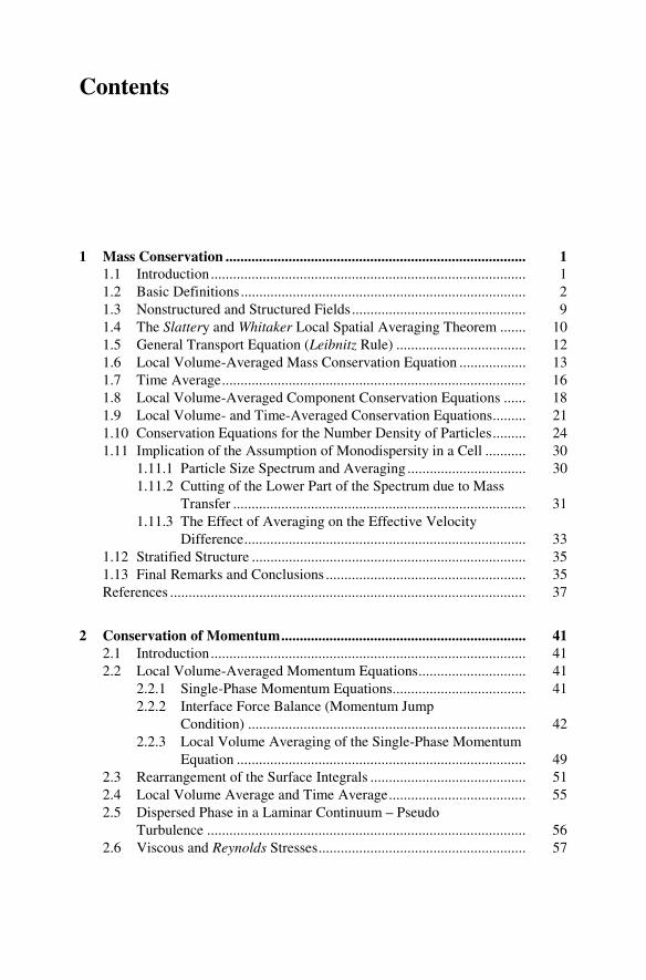
1 Mass Conservation ................................................................................. 1 1.1 Introduction ..................................................................................... 1 1.2 Basic Definitions ............................................................................. 2 1.3 Nonstructured and Structured Fields ............................................... 9 1.4 The Slattery and Whitaker Local Spatial Averaging Theorem ....... 10 1.5 General Transport Equation (Leibnitz Rule) ................................... 12 1.6 Local Volume-Averaged Mass Conservation Equation .................. 13 1.7 Time Average .................................................................................. 16 1.8 Local Volume-Averaged Component Conservation Equations ...... 18 1.9 Local Volume- and Time-Averaged Conservation Equations ......... 21 1.10 Conservation Equations for the Number Density of Particles ......... 24 1.11 Implication of the Assumption of Monodispersity in a Cell ........... 30

1.11.1 Particle Size Spectrum and Averaging ................................ 30 1.11.2 Cutting of the Lower Part of the Spectrum due to Mass

Transfer ............................................................................... 31 1.11.3 The Effect of Averaging on the Effective Velocity

Difference ............................................................................ 33 1.12 Stratified Structure .......................................................................... 35 1.13 Final Remarks and Conclusions ...................................................... 35 References ................................................................................................ 37

2 Conservation of Momentum .................................................................. 41 2.1 Introduction ..................................................................................... 41 2.2 Local Volume-Averaged Momentum Equations ............................. 41

2.2.1 Single-Phase Momentum Equations.................................... 41 2.2.2 Interface Force Balance (Momentum Jump

Condition) ........................................................................... 42 2.2.3 Local Volume Averaging of the Single-Phase Momentum

Equation .............................................................................. 49 2.3 Rearrangement of the Surface Integrals .......................................... 51 2.4 Local Volume Average and Time Average ..................................... 55 2.5 Dispersed Phase in a Laminar Continuum – Pseudo

Turbulence ...................................................................................... 56 2.6 Viscous and Reynolds Stresses ........................................................ 57

XXVI Contents

2.7 Nonequal Bulk and Boundary Layer Pressures ............................... 62 2.7.1 Continuous Interface ........................................................... 62 2.7.2 Dispersed Interface .............................................................. 76

2.8 Working form for the Dispersed and Continuous Phase ................. 92 2.9 General Working form for Dispersed and Continuous Phases ........ 97 2.10 Some Practical Simplifications ....................................................... 99 2.11 Conclusion ...................................................................................... 103 Appendix 2.1 ............................................................................................ 104 Appendix 2.2 ............................................................................................ 105 Appendix 2.3 ............................................................................................ 105 References ................................................................................................ 110

3 Derivatives for the Equations of State .................................................. 117 3.1 Introduction ..................................................................................... 117 3.2 Multi-component Mixtures of Miscible and Non-miscible

Components .................................................................................... 119 3.2.1 Computation of Partial Pressures for Known Mass

Concentrations, System Pressure and Temperature............. 121 3.2.2 Partial Derivatives of the Equation of State

........................................................... 127 3.2.3 Partial Derivatives in the Equation of State

, where .............................. 133 3.2.4 Chemical Potential .............................................................. 142 3.2.5 Partial Derivatives in the Equation of State

, where .............................. 152 3.3 Mixture of Liquid and Microscopic Solid Particles of

Different Chemical Substances ....................................................... 155 3.3.1 Partial Derivatives in the Equation of State

........................................................... 155 3.3.2 Partial Derivatives in the Equation of State

where ............................... 156

3.4 Single-Component Equilibrium Fluid ............................................. 157 3.4.1 Superheated Vapor .............................................................. 157 3.4.2 Reconstruction of Equation of State by Using a Limited

Amount of Data Available .................................................. 159 3.4.3 Vapor-Liquid Mixture in Thermodynamic Equilibrium ...... 166 3.4.4 Liquid-Solid Mixture in Thermodynamic Equilibrium ....... 166 3.4.5 Solid Phase .......................................................................... 167

3.5 Extension State of Liquids .............................................................. 167

( )max2,...,, , ip T Cρ ρ=

( )max2,...,, , iT T p Cϕ= , ,s h eϕ =

( )max2,...,, , ip Cρ ρ ϕ= , ,s h eϕ =

( )max2,...,, , ip T Cρ ρ=

( )max2,...,, , iT T p Cϕ= , ,h e sϕ =

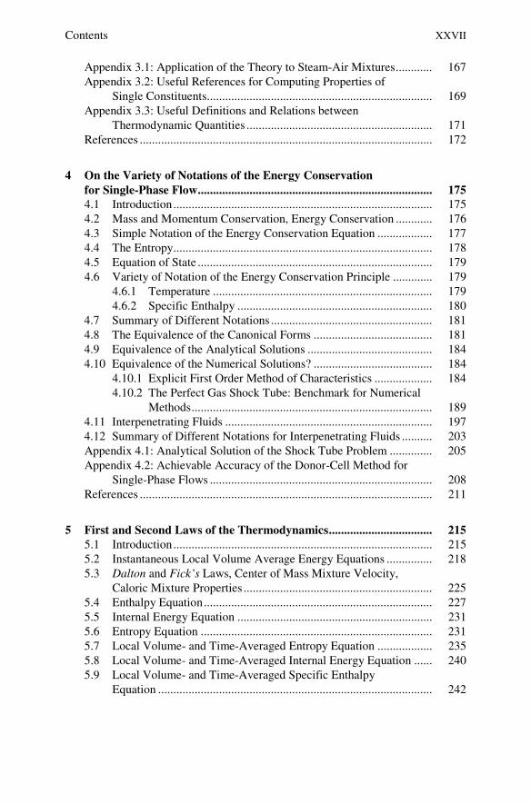
Contents XXVII

Appendix 3.1: Application of the Theory to Steam-Air Mixtures ............ 167 Appendix 3.2: Useful References for Computing Properties of

Single Constituents.......................................................................... 169 Appendix 3.3: Useful Definitions and Relations between

Thermodynamic Quantities ............................................................. 171 References ................................................................................................ 172

4 On the Variety of Notations of the Energy Conservation for Single-Phase Flow ............................................................................. 175 4.1 Introduction ..................................................................................... 175 4.2 Mass and Momentum Conservation, Energy Conservation ............ 176 4.3 Simple Notation of the Energy Conservation Equation .................. 177 4.4 The Entropy ..................................................................................... 178 4.5 Equation of State ............................................................................. 179 4.6 Variety of Notation of the Energy Conservation Principle ............. 179

4.6.1 Temperature ........................................................................ 179 4.6.2 Specific Enthalpy ................................................................ 180

4.7 Summary of Different Notations ..................................................... 181 4.8 The Equivalence of the Canonical Forms ....................................... 181 4.9 Equivalence of the Analytical Solutions ......................................... 184 4.10 Equivalence of the Numerical Solutions? ....................................... 184

4.10.1 Explicit First Order Method of Characteristics ................... 184 4.10.2 The Perfect Gas Shock Tube: Benchmark for Numerical

Methods ............................................................................... 189 4.11 Interpenetrating Fluids .................................................................... 197 4.12 Summary of Different Notations for Interpenetrating Fluids .......... 203 Appendix 4.1: Analytical Solution of the Shock Tube Problem .............. 205 Appendix 4.2: Achievable Accuracy of the Donor-Cell Method for

Single-Phase Flows ......................................................................... 208 References ................................................................................................ 211

5 First and Second Laws of the Thermodynamics .................................. 215 5.1 Introduction ..................................................................................... 215 5.2 Instantaneous Local Volume Average Energy Equations ............... 218 5.3 Dalton and Fick’s Laws, Center of Mass Mixture Velocity,

Caloric Mixture Properties .............................................................. 225 5.4 Enthalpy Equation ........................................................................... 227 5.5 Internal Energy Equation ................................................................ 231 5.6 Entropy Equation ............................................................................ 231 5.7 Local Volume- and Time-Averaged Entropy Equation .................. 235 5.8 Local Volume- and Time-Averaged Internal Energy Equation ...... 240 5.9 Local Volume- and Time-Averaged Specific Enthalpy

Equation .......................................................................................... 242

XXVIII Contents

5.10 Non-Conservative and Semi-Conservative Forms of the Entropy Equation ............................................................................ 244

5.11 Comments on the Source Terms in the Mixture Entropy Equation .......................................................................................... 246

5.12 Viscous Dissipation ......................................................................... 250 5.13 Temperature Equation ..................................................................... 256 5.14 Second Law of the Thermodynamics .............................................. 260 5.15 Mixture Volume Conservation Equation ........................................ 261 5.16 Linearized Form of the Source Term for the Temperature

Equation .......................................................................................... 266 5.17 Interface Conditions ........................................................................ 273 5.18 Lumped Parameter Volumes ........................................................... 274 5.19 Steady State ..................................................................................... 275 5.20 Final Remarks ................................................................................. 281 References ................................................................................................ 282

6 Some Simple Applications of Mass and Energy Conservation ........... 285 6.1 Infinite Heat Exchange without Interfacial Mass Transfer.............. 285 6.2 Discharge of Gas from a Volume .................................................... 287 6.3 Injection of Inert Gas in a Closed Volume Initially Filled with

Inert Gas .......................................................................................... 289 6.4 Heat Input in a Gas in a Closed Volume ......................................... 290 6.5 Steam Injection in a Steam-Air Mixture ......................................... 291 6.6 Heat Removal from a Closed Volume Containing Equilibrium

Two-Phase Mixture ......................................................................... 294 6.7 Chemical Reaction in a Gas Mixture in a Closed Volume .............. 297 6.8 Hydrogen Combustion in an Inert Atmosphere ............................... 299

6.8.1 Simple Introduction to Combustion Kinetics ...................... 299 6.8.2 Ignition Temperature and Ignition Concentration

Limits .................................................................................. 301 6.8.3 Detonability Concentration Limits ...................................... 302 6.8.4 The Heat Release Due to Combustion ................................. 302 6.8.5 Equilibrium Dissociation ..................................................... 304 6.8.6 Source Terms of the Energy Conservation of the Gas

Phase ................................................................................... 308 6.8.7 Temperature and Pressure Changes in a Closed Control

Volume; Adiabatic Temperature of the Burned Gases ........ 310 6.9 Constituents of Sodium Vapor ........................................................ 314 References ................................................................................................ 318

7 Exergy of Multi-phase Multi-component Systems ............................... 321 7.1 Introduction ..................................................................................... 321 7.2 The Pseudo-exergy Equation for Single-Fluid Systems .................. 321 7.3 The Fundamental Exergy Equation ................................................. 323

Contents XXIX

7.3.1 The Exergy Definition in Accordance with Reynolds and Perkins .......................................................................... 323

7.3.2 The Exergy Definition in Accordance with Gouy (l’énergie utilisable, 1889) .................................................. 324

7.3.3 The Exergy Definition Appropriate for Estimation of the Volume Change Work ............................................... 325

7.3.4 The Exergy Definition Appropriate for Estimation of the Technical Work ......................................................... 326

7.4 Some Interesting Consequences of the Fundamental Exergy Equation .......................................................................................... 326

7.5 Judging the Efficiency of a Heat Pump as an Example of Application of the Exergy ............................................................... 328

7.6 Three-Fluid Multi-component Systems ........................................... 329 7.7 Practical Relevance ......................................................................... 333 References ................................................................................................ 333

8 One-Dimensional Three-Fluid Flows .................................................... 335 8.1 Summary of the Local Volume- and Time-Averaged

Conservation Equations .................................................................. 335 8.2 Treatment of the Field Pressure Gradient Forces ............................ 338

8.2.1 Dispersed Flows .................................................................. 338 8.2.2 Stratified Flow ..................................................................... 339

8.3 Pipe Deformation Due to Temporal Pressure Change in the Flow ...................................................................................... 339

8.4 Some Simple Cases ......................................................................... 341 8.5 Slip Model – Transient Flow ........................................................... 348 8.6 Slip Model – Steady State. Critical Mass Flow Rate ...................... 352 8.7 Forces Acting on the Pipes Due to the Flow – Theoretical

Basics .............................................................................................. 360 8.8 Relief Valves ................................................................................... 367

8.8.1 Introduction ......................................................................... 367 8.8.2 Valve Characteristics, Model Formulation .......................... 368 8.8.3 Analytical Solution .............................................................. 372 8.8.4 Fitting the Piecewise Solution on Two Known Position –

Time Points ......................................................................... 374 8.8.5 Fitting the Piecewise Solution on Known Velocity and

Position for a Given Time ................................................... 376 8.8.6 Idealized Valve Characteristics ........................................... 377 8.8.7 Recommendations for the Application of the Model

in System Computer Codes ................................................. 379 8.8.8 Some Illustrations of the Valve Performance Model .......... 381 8.8.9 Nomenclature for Section 8.8 .............................................. 387

8.9 Pump Model .................................................................................... 389 8.9.1 Variables Defining the Pump Behavior ............................... 389

XXX Contents

8.9.2 Theoretical Basics ............................................................... 392 8.9.3 Suter Diagram ..................................................................... 401 8.9.4 Computational Procedure .................................................... 407 8.9.5 Centrifugal Pump Drive Model ........................................... 408 8.9.6 Extension of the Theory to Multiphase Flow ...................... 409

Appendix 1: Chronological References to the Subject Critical Two-Phase Flow.............................................................................. 413

References ................................................................................................ 419

9 Detonation Waves Caused by Chemical Reactions or by Melt-coolant Interactions ............................................................................................. 421 9.1 Introduction ..................................................................................... 421 9.2 Single-Phase Theory ....................................................................... 423

9.2.1 Continuum Sound Waves (Laplace) ................................... 423 9.2.2 Discontinuum Shock Waves (Rankine-Hugoniot) .............. 424 9.2.3 The Landau and Liftshitz Analytical Solution for

Detonation in Perfect Gases ................................................ 428 9.2.4 Numerical Solution for Detonation in Closed Pipes ........... 432

9.3 Multi-phase Flow ............................................................................ 435 9.3.1 Continuum Sound Waves .................................................... 435 9.3.2 Discontinuous Shock Waves ............................................... 437 9.3.3 Melt–coolant Interaction Detonations ................................. 441 9.3.4 Similarity to and Differences from the Yuen and

Theofanous Formalism ........................................................ 446 9.3.5 Numerical Solution Method ................................................ 446

9.4 Detonation Waves in Water Mixed with Different Molten Materials.......................................................................................... 447 9.4.1 UO2 Water System .............................................................. 448 9.4.2 Efficiencies .......................................................................... 452 9.4.3 The Maximum Coolant Entrainment Ratio ......................... 455

9.5 Conclusions ..................................................................................... 456 9.6 Practical Significance ...................................................................... 458 Appendix 9.1: Specific Heat Capacity at Constant Pressure for Urania

and Alumina .................................................................................... 459 References ................................................................................................ 460

10 Conservation Equations in General Curvilinear Coordinate Systems .................................................................................................... 463 10.1 Introduction ..................................................................................... 463 10.2 Field Mass Conservation Equations ................................................ 464 10.3 Mass Conservation Equations for Components Inside

the Field – Conservative Form ........................................................ 467 10.4 Field Mass Conservation Equations for Components Inside

the Field – Non-conservative Form ................................................. 469

Contents XXXI

10.5 Particles Number Conservation Equations for Each Velocity Field ................................................................................................ 469

10.6 Field Entropy Conservation Equations – Conservative Form ......... 470 10.7 Field Entropy Conservation Equations – Non-conservative

Form ................................................................................................ 471 10.8 Irreversible Power Dissipation Caused by the Viscous Forces ....... 471 10.9 The Non-conservative Entropy Equation in Terms of Temperature

and Pressure .................................................................................... 473 10.10 The Volume Conservation Equation ............................................... 475 10.11 The Momentum Equations .............................................................. 477 10.12 The Flux Concept, Conservative and Semi-conservative

Forms .............................................................................................. 484 10.12.1 Mass Conservation Equation .............................................. 484 10.12.2 Entropy Equation ................................................................ 486 10.12.3 Temperature Equation ......................................................... 486 10.12.4 Momentum Conservation in the x-Direction ...................... 487 10.12.5 Momentum Conservation in the y-Direction ...................... 488 10.12.6 Momentum Conservation in the z-Direction ....................... 490

10.13 Concluding Remarks ....................................................................... 491 References ................................................................................................ 491

11 Type of the System of PDEs ................................................................... 493 11.1 Eigenvalues, Eigenvectors, Canonical Form ................................... 493 11.2 Physical Interpretation .................................................................... 496

11.2.1 Eigenvalues and Propagation Velocity of Perturbations ..... 496 11.2.2 Eigenvalues and Propagation Velocity of Harmonic

Oscillations .......................................................................... 496 11.2.3 Eigenvalues and Critical Flow ............................................ 497

References ................................................................................................ 498

12 Numerical Solution Methods for Multi-phase Flow Problems ........... 499 12.1 Introduction ..................................................................................... 499 12.2 Formulation of the Mathematical Problem...................................... 499 12.3 Space Discretization and Location of the Discrete Variables ......... 501 12.4 Discretization of the Mass Conservation Equations ........................ 506 12.5 First Order Donor-Cell Finite Difference Approximations ............. 508 12.6 Discretization of the Concentration Equations ................................ 510 12.7 Discretization of the Entropy Equation ........................................... 511 12.8 Discretization of the Temperature Equation .................................... 512 12.9 Physical Significance of the Necessary Convergence

Condition ......................................................................................... 515

XXXII Contents

12.10 Implicit Discretization of Momentum Equations ............................ 517 12.11 Pressure Equations for IVA2 and IVA3 Computer Codes .............. 523 12.12 A Newton-type Iteration Method for Multi-phase Flows ................ 527 12.13 Integration Procedure: Implicit Method .......................................... 536 12.14 Time Step and Accuracy Control .................................................... 537 12.15 High Order Discretization Schemes for Convection-Diffusion

Terms .............................................................................................. 539 12.15.1 Space Exponential Scheme ................................................. 539 12.15.2 High Order Upwinding ....................................................... 542 12.15.3 Constrained Interpolation Profile (CIP) Method ................. 544

12.16 Problem Solution Examples to the Basics of the CIP Method ........ 548 12.16.1 Discretization Concept ........................................................ 548 12.16.2 Second Order Constrained Interpolation Profiles ............... 549 12.16.3 Third Order Constrained Interpolation Profiles .................. 551 12.16.4 Fourth Order Constrained Interpolation Profiles ................ 552

12.17 Pipe Networks: Some Basic Definitions ......................................... 572 12.17.1 Pipes .................................................................................... 573 12.17.2 Axis in the Space ................................................................ 574 12.17.3 Diameters of Pipe Sections ................................................. 576 12.17.4 Reductions .......................................................................... 576 12.17.5 Elbows ................................................................................ 577 12.17.6 Creating a Library of Pipes ................................................. 577 12.17.7 Sub System Network........................................................... 577 12.17.8 Discretization of Pipes ........................................................ 578 12.17.9 Knots ................................................................................... 579

Appendix 12.1: Definitions Applicable to Discretization of the Mass Conservation Equations ............................................... 581

Appendix 12.2: Discretization of the Concentration Equations ............... 583 Appendix 12.3: Harmonic Averaged Diffusion Coefficients ................... 586 Appendix 12.4: Discretized Radial Momentum Equation ........................ 587 Appendix 12.5: The Coefficients for Eq. (12.46) ............................... 592 Appendix 12.6: Discretization of the Angular Momentum

Equation .......................................................................................... 592 Appendix 12.7: Discretization of the Axial Momentum Equation ........... 594 Appendix 12.8: Analytical Derivatives for the Residual Error

of Each Equation with Respect to the Dependent Variables ........... 596 Appendix 12.9: Simple Introduction to Iterative Methods

for Solution of Algebraic Systems .................................................. 599 References ................................................................................................ 600

13 Numerical Methods for Multi-phase Flow in Curvilinear Coordinate Systems .................................................................................................... 607 13.1 Introduction ..................................................................................... 607 13.2 Nodes, Grids, Meshes, Topology – Some Basic Definitions .......... 609

a

Contents XXXIII

13.3 Formulation of the Mathematical Problem...................................... 610 13.4 Discretization of the Mass Conservation Equations ........................ 612

13.4.1 Integration Over a Finite Time Step and Finite Control Volume ................................................................................ 612

13.4.2 The Donor-Cell Concept ..................................................... 614 13.4.3 Two Methods for Computing the Finite Difference

Approximations of the Contravariant Vectors at the Cell Center .......................................................................... 617

13.4.4 Discretization of the Diffusion Terms ................................. 619 13.5 Discretization of the Entropy Equation ........................................... 623 13.6 Discretization of the Temperature Equation .................................... 624 13.7 Discretization of the Particle Number Density Equation ................ 624 13.8 Discretization of the x Momentum Equation .................................. 625 13.9 Discretization of the y Momentum Equation .................................. 627 13.10 Discretization of the z Momentum Equation ................................... 627 13.11 Pressure-Velocity Coupling ............................................................ 628 13.12 Staggered x Momentum Equation ................................................... 633 Appendix 13.1: Harmonic Averaged Diffusion Coefficients ................... 643 Appendix 13.2: Off-Diagonal Viscous Diffusion Terms of the

x Momentum Equation .................................................................... 645 Appendix 13.3: Off-Diagonal Viscous Diffusion Terms of the

y Momentum Equation .................................................................... 648 Appendix 13.4: Off-Diagonal Viscous Diffusion Terms of the z

Momentum Equation ....................................................................... 650 References ................................................................................................ 653

14 Conservation Equations in the Relative Coordinate System ............. 657 14.1 Conservation of Scalars ................................................................... 657 14.2 Entropy Equation ............................................................................ 659 14.3 Momentum Equation ....................................................................... 660

14.3.1 Single Phase Flow, Vector Notation ................................... 660 14.3.2 Scalar Notation, Multiphase Flow ....................................... 664

14.4 Angular Momentum Conservation .................................................. 667 14.5 Conservation of Rotation Energy .................................................... 669

14.5.1 Rothalpy .............................................................................. 672 14.5.2 Isentropic Energy Transfer from the Flow to the

Blades .................................................................................. 673 14.5.3 Non Isentropic Energy Dissipation ..................................... 673 14.5.4 Rotor Stage Power ............................................................... 679 14.5.2 Tangential Blade Forces ...................................................... 683 14.5.3 Axial Blade Forces .............................................................. 684

14.6 Example of the Application of the Axial Turbine Model ................ 687 14.7 The Energy Jump Across Stator/Rotor Interfaces ........................... 689

XXXIV Contents

14.7.1 Energy Jump Approach ....................................................... 689 14.7.2 Continuum Approach .......................................................... 689

14.8 Steady Flow Expansion: Single Phase; Two Phase Equilibrium..... 690 14.9 Transient Turbo-Generator Behavior .............................................. 702 Appendix 14.1 .......................................................................................... 703 Appendix 14.2: Streamline Momentum Conservation in the Stator ......... 705 Nomenclature ........................................................................................... 708 References ................................................................................................ 709

15 Visual Demonstration of the Method .................................................... 711 15.1 Melt-Water Interactions .................................................................. 711

15.1.1 Cases 1 to 4 ......................................................................... 711 15.1.2 Cases 5, 6 and 7 ................................................................... 717 15.1.3 Cases 8 to 10 ....................................................................... 721 15.1.4 Cases 11 and 12 ................................................................... 732 15.1.5 Case 13 ................................................................................ 734 15.1.6 Case 14 ................................................................................ 736

15.2 Pipe Networks ................................................................................. 738 15.3 3D Steam-Water Interactions .......................................................... 740 15.4 Three-Dimensional Steam-Water Interaction in Presence

of Non-Condensable Gases ............................................................. 741 15.4.1 Case 17 ................................................................................ 741

15.5 Three Dimensional Steam Production in Boiling Water Reactor ............................................................................................ 743 15.5.1 Case 18 ................................................................................ 743

References ................................................................................................ 744

Appendix 1: Brief Introduction to Vector Analysis ................................... 747

Appendix 2: Basics of the Coordinate Transformation Theory ............... 775

Subject Index................................................................................................. 831

Nomenclature

Latin

A cross-section, m² A surface vector a speed of sound, /m s

lwa surface of the field l wetting the wall w per unit flow volume max

1

l

ll

Vol=∑

belonging to control volume Vol (local volume interface area density of the structure w), 1m−

la σ surface of the velocity field l contacting the neighboring fields per unit

flow volume max

1

l

ll

Vol=∑ belonging to control volume Vol (local volume

interface area density of the velocity field l), 1m−

la total surface of the velocity field l per unit flow volume max

1

l

ll

Vol=∑

belonging to control volume Vol (local volume interface area density of the velocity field l), 1m−

iCu Courant criterion corresponding to each eigenvalue, dimensionless

ilC mass concentration of the inert component i in the velocity field l

c coefficients, dimensionless

mC mass concentration of the component m in the velocity field,

dimensionless

iC mass concentration of the component i in the velocity field, dimensionless

pc specific heat at constant pressure, ( )/J kgK vmc virtual mass force coefficient, dimensionless dc drag force coefficient, dimensionless Lc lift force coefficient, dimensionless

hyD hydraulic diameter (4 times cross-sectional area / perimeter), m

3ED diameter of the entrained droplets, m

XXXVI Nomenclature

ldD size of the bubbles produced after one nucleation cycle on the solid

structure, bubble departure diameter, m

1dmD size of bubbles produced after one nucleation cycle on the inert solid

particles of field m = 2, 3

lchD critical size for homogeneous nucleation, m

lcdD critical size in presence of dissolved gases, m

lD′ most probable particle size, m

lD characteristic length of the velocity field l, particle size in case of

fragmented field, m lilD coefficient of molecular diffusion for species i into the field l, 2 /m s tilD coefficient of turbulent diffusion, 2 /m s *ilD total diffusion coefficient, 2 /m s

ilDC right-hand side of the nonconservative conservation equation for the inert

component, ( )3/kg sm

D diffusivity, 2 /m s d total differential E total energy, J e specific internal energy, J/kg

( )F ξ function introduced first in Eq. (42), Chapter 2

, (...F f function of (...

f force per unit flow volume, 3/N m f fraction of entrained melt or water in the detonation theory

lwF surfaces separating the velocity field l from the neighboring structure

within Vol, 2m

lFσ surfaces separating the velocity field l from the neighboring velocity field

within Vol, 2m

F surface defining the control volume Vol, 2m

imf frequency of the nuclei generated from one activated seed on the particle

belonging to the donor velocity field m, 1s−

lwf frequency of the bubble generation from one activated seed on the

channel wall, 1s−

,l coalf coalescence frequency, 1s−

g acceleration due to gravity, 2/m s H height, m h specific enthalpy, J/kg

ih eigenvectors corresponding to each eigenvalue

I unit matrix, dimensionless i unit vector along the x-axis

Nomenclature XXXVII

J matrix, Jacobian j unit vector along the y-axis k unit vector along the k-axis k cell number k kinetic energy of turbulent pulsation, 2 2/m s

Tilk coefficient of thermodiffusion, dimensionless p

ilk coefficient of barodiffusion, dimensionless

L length, m

iM kg-mole mass of the species i, kg/mole

m total mass, kg

ΔVn unit vector pointing along mlΔV , dimensionless

n unit vector pointing outwards from the control volume Vol, dimensionless

len unit surface vector pointing outwards from the control volume Vol

lσn unit interface vector pointing outwards from the velocity field l

iln number of the particle from species i per unit flow volume, 3m−

ln number of particles of field i per unit flow volume, particle number

density of the velocity field l, 3m−

coaln number of particles disappearing due to coalescence per unit time and

unit volume, 3m−

,l kinn particle production rate due to nucleation during evaporation or

condensation, ( )31/ m s

lwn′′ number of the activated seeds on unit area of the wall, m−2

lhn number of the nuclei generated by homogeneous nucleation in the donor

velocity field per unit time and unit volume of the flow, ( )31/ m s

,l disn number of the nuclei generated from dissolved gases in the donor velocity

field per unit time and unit volume of the flow, ( )31/ m s

,l spn number of particles of the velocity field l arising due to hydrodynamic

disintegration per unit time and unit volume of the flow, ( )31/ m s

P probability P irreversibly dissipated power from the viscous forces due to deformation

of the local volume and time average velocities in the space, /W kg

Per perimeter, m

lip l = 1: partial pressure inside the velocity field l

l = 2,3: pressure of the velocity field l p pressure, Pa q′′′ thermal power per unit flow volume introduced into the fluid, 3/W m

XXXVIII Nomenclature

lqσ′′′ l = 1,2,3. Thermal power per unit flow volume introduced from the

interface into the velocity field l, 3/W m

w lq σ′′′ thermal power per unit flow volume introduced from the structure

interface into the velocity field l, 3/W m R mean radius of the interface curvature, m r(x,y,z) position vector, m R (with indexes) gas constant, J/(kgK) s arc length vector, m S total entropy, J/K s specific entropy, J/(kgK)

tSc turbulent Schmidt number, dimensionless tnSc is the turbulent Schmidt number for particle diffusion, dimensionless

T temperature, K

lT temperature of the velocity field l, K

T shear stress tensor, 2/N m t unit tangent vector U dependent variables vector Vol control volume, 3m

1/ 3Vol size of the control volume, m

lVol volume available for the field l inside the control volume, 3m max

1

l

ll

Vol=∑ volume available for the flow inside the control volume, 3m

V instantaneous fluid velocity with components, u, v, w in , ,r θ and zdirection, m/s

lτV instantaneous field velocity with components, , ,l l lu v wϑ τ τ in , ,r θ and z

direction, m/s

lV time-averaged velocity, m/s

l′V pulsation component of the instantaneous velocity field, m/s

lmΔV l m−V V , velocity difference, disperse phase l, continuous phase m

carrying l, /m s

i lV τδ diffusion velocity, m/s

lτσV interface velocity vector, m/s

lτ γV instantaneous vector with components, , ,l r l l zu v wϑ τ τ

θγ γ γ in , ,r θ and zdirections, m/s

v specific volume, 3 /m kg

x mass fraction, dimensionless y distance between the bottom of the pipe and the center of mass of the

liquid, m × vector product

Nomenclature XXXIX

Greek

lα part of vVolγ available to the velocity field l, local instantaneous volume

fraction of the velocity field l, dimensionless

ilα the same as lα in the case of gas mixtures; in the case of mixtures

consisting of liquid and macroscopic solid particles, the part of vVolγ

available to the inert component i of the velocity field l, local instantaneous volume fraction of the inert component i of the velocity field l, dimensionless

,maxlα 0.62≈ , limit for the closest possible packing of particles, dimensionless

vγ the part of dVol available for the flow, volumetric porosity, dimensionless

γ surface permeability, dimensionless

γ directional surface permeability with components , ,r zθγ γ γ ,

dimensionless Δ finite difference δ small deviation with respect to a given value

lδ = 1 for continuous field;

= 0 for disperse field, dimensionless ∂ partial differential ε dissipation rate for kinetic energy from turbulent fluctuation, power

irreversibly dissipated by the viscous forces due to turbulent fluctuations, /W kg

η dynamic viscosity, kg/(ms)

θ θ -coordinate in the cylindrical or spherical coordinate systems, rad κ = 0 for Cartesian coordinates, = 1 for cylindrical coordinates κ isentropic exponent

lκ curvature of the surface of the velocity field l, m

λ thermal conductivity, W/(mK) λ eigenvalue

lτμ local volume-averaged mass transferred into the velocity field l per unit

time and unit mixture flow volume, local volume-averaged instantaneous

mass source density of the velocity field l, ( )3/kg m s

lμ time average of lτμ , ( )3/kg m s

wlμ mass transport from exterior source into the velocity field l, ( )3/kg m s

ilτμ local volume-averaged inert mass from species i transferred into the velocity

field l per unit time and unit mixture flow volume, local volume-averaged instantaneous mass source density of the inert component i of the velocity

field l, ( )3/kg m s

XL Nomenclature

ilμ time average of ilτμ , ( )3/kg m s

imlτμ local volume-averaged instantaneous mass source density of the inert

component i of the velocity field l due to mass transfer from field m,

( )3/kg m s

imlμ time average of imlτμ , ( )3/kg m s

ilmτμ local volume-averaged instantaneous mass source density of the inert

component i of the velocity field l due to mass transfer from field l into

velocity field m, ( )3/kg m s

ilmμ time average of ilmτμ , ( )3/kg m s

ν cinematic viscosity, 2 /m s

ν lt coefficient of turbulent cinematic viscosity, 2 /m s

tnlν coefficient of turbulent particles diffusion, 2 /m s

ξ angle between lσn and lmΔV , rad

ρ density, kg/m3

ρ instantaneous density, density; without indexes, mixture density, kg/m3

lρ instantaneous field density, kg/m3

ilρ instantaneous inert component density of the velocity field l, kg/m3 l

lρ intrinsic local volume-averaged phase density, kg/m3

( )23

wρ entrainment mass flow rate, ( )2/kg m s

( )32

wρ deposition mass flow rate, ( )2/kg m s

( )lel lτρ V local intrinsic surface mass flow rate, ( )2/kg m s

σ , 12σ surface tension between phases 1 and 2, N/m

τ time, s ϕ angle giving the projection of the position of the surface point in the

plane normal to lmΔV , rad mlσχ the product of the effective heat transfer coefficient and the interfacial

area density, ( )3/W m K . The subscript l denotes inside the velocity field

l. The superscript mσ denotes location at the interface σ dividing field m from field l. The superscript is only used if the interfacial heat transfer is associated with mass transfer. If there is heat transfer only, the linearized interaction coefficient is assigned the subscript ml only, indicating the interface at which the heat transfer takes place.

Nomenclature XLI

Subscripts

c continuous d disperse lm from l to m or l acting on m w region "outside of the flow" e entrances and exits for control volume Vol l velocity field l, intrinsic field average i inert components inside the field l, noncondensable gases in the gas field

l = 1, or microscopic particles in water in field 2 or 3 i corresponding to the eigenvalue iλ in Chapter 4

M noninert component m mixture of entrained coolant and entrained melt debris that is in thermal

and mechanical equilibrium behind the shock front ml from m into l iml from im into il max maximum number of points n inert component 0 at the beginning of the time step E entrainment coal coalescence sp splitting, fragmentation σ interface τ old time level τ τ+Δ new time level * initial 0 reference conditions p,v,s at constant p,v,s, respectively L left R right 1 vapor or in front of the shock wave 2 water or behind the shock wave 3 melt 4 entrained coolant behind the front – entrained coolant 5 microparticles after the thermal interaction – entrained melt Superscripts

´ time fluctuation

' saturated steam " saturated liquid "' saturated solid phase A air d drag

XLII Nomenclature

e heterogeneous i component (either gas or solid particles) of the velocity field

maxi maximum for the number of the components inside the velocity field

L lift l intrinsic field average le intrinsic surface average lσ averaged over the surface of the sphere m component n normal n old iteration n+1 new iteration t turbulent, tangential vm virtual mass τ temporal, instantaneous

averaging sign

Operators ∇⋅ divergence ∇ gradient

n∇ normal component of the gradient

t∇ tangential component of the gradient

l∇ surface gradient operator, 1/m 2∇ Laplacian

local volume average l local intrinsic volume average

le local intrinsic surface average

Nomenclature required for coordinate transformations

( ), ,x y z coordinates of a Cartesian, left oriented coordinate system (Euclidean

space). Another notation which is simultaneously used is ix ( )1, 2,3i = :

1 2 3, ,x x x

( ), ,ξ η ζ coordinates of the curvilinear coordinate system called transformed

coordinate system. Another notation which is simultaneously used is iξ

( )1, 2,3i = : 1 2 3, ,ξ ξ ξ

csV the velocity of the curvilinear coordinate system

Nomenclature XLIII

g Jacobian determinant or Jacobian of the coordinate transformation

( ), ,x f ξ η ζ= , ( ), ,y g ξ η ζ= , ( ), ,z h ξ η ζ=

ija elements of the Jacobian determinant ija elements of the determinant transferring the partial derivatives with

respect to the transformed coordinates into partial derivatives with respect to the physical coordinates. The second superscript indicates the Cartesian components of the contravariant vectors

( )1 2 3, ,a a a covariant base vectors of the curvilinear coordinate system tangent

vectors to the three curvilinear coordinate lines represented by

( ), ,ξ η ζ

( )1 2 3, ,a a a contravariant base vectors, normal to a coordinate surface on which

the coordinates ξ , η and ζ are constant, respectively

ijg covariant metric tensor (symmetric) ijg contravariant metric tensor (symmetric)

( )1 2 3, ,e e e unit vectors normal to a coordinate surface on which the coordinates

ξ , η and ζ are constant, respectively iV i= ⋅a V , contravariant components of the vector V i= ⋅a V , covariant components of the vector V

( ), ,ξ η ζγ γ γ permeabilities of coordinate surfaces on which the coordinates ξ , η

and ζ are constant, respectively

Greek

Α , α Alpha Β , β Beta

Γ , γ Gamma

Δ , δ Delta Ε , ε Epsilon Ζ , ζ Zeta

Η , η Eta

Θ , ϑ Theta

Ι , ι Iota Κ , κ Kappa Λ , λ Lambda Μ , μ Mu

Ν , ν Nu Ξ ,ξ Xi

Ο , ο Omikron Π , π Pi Ρ , ρ Rho

Σ , σ Sigma Τ , τ Tau Φ , ϕ Phi

Χ , χ Chi

ϒ , υ Ypsilon Ψ , ψ Psi

Ω , ω Omega

iV