Multiobjective Mixed-Integer Stackelberg Gamescoral.ie.lehigh.edu/~ted/files/talks/LBMZSSPIC-EURO06.pdf · mixed-integer zero-sum static Stackelberg problem (MZSSP): MZSSP min x

Stackelberg GamesBiobjective Programs

Solving the LBMZSSPICConclusionReferences

Multiobjective Mixed-Integer Stackelberg Games

SCOTT DENEGRETED RALPHS

ISE DepartmentCOR@L Lab

Lehigh [email protected]

EURO XXI, Reykjavic, Iceland

July 3, 2006

Denegre & Ralphs LBMZSSPIC



Outline

1 Stackelberg GamesGeneral SetupZero-sum Stackelberg GamesMixed-Integer Stackelberg Games

2 Biobjective ProgramsOverviewSolution Techniques

3 Solving the LBMZSSPICUsing the WCN AlgorithmSolving the SubproblemsA Branch and Bound Algorithm

4 Conclusion




General SetupZero-sum Stackelberg GamesMixed-Integer Stackelberg Games

Basic Setup

We wish to study the following type of two-player game:

Scenario

There are two players, a leader and a follower.

Each player controls the level of certain activities subject toconstraints and seeks to optimize a given objective function.

The leader sets activity levels first.

The follower then reacts based on the choices of the leader.

The leader can affect the follower through constraints on the followerthat involve the leader’s choices.

This is an example of what are generally known in the literature asStackelberg games.

Here, we consider static games in which there is only one round ofdecision-making.

We can model such games mathematically as bilevel programs.





Bilevel Programs

Suppose the variables x and y represent the activities controlled by theleader and follower, respectively.A bilevel program is a standard mathematical program with y constrainedto be optimal for the secondary program

min f (x, y) : h(x, y) ≤ 0 .

This yields the (continuous) bilevel programming problem (BPP):

A Bilevel Program

minx,y

F(x, y)

subject to g(x, y) ≤ 0 (1)

y ∈ argmin f (x, y) : h(x, y) ≤ 0

Bilevel programs are known to be NP-hard, even if all functions arelinear [Calamai and Vincente, 1994, Jeroslow, 1985, Ben-Ayed andBlair, 1990, Hansen et al., 1992].





Underlying Assumptions

Implicit in formulation (1) are the following basic assumptions:

Assumptions

1 Perfect information: Each player has perfect information about theother’s actions and strategy.

2 Rationality: Both players act optimally.3 Determinism: Each player chooses deterministically among

alternative optima.

Assumption 3 is necessary in order for (1) to be well-defined.

The presence of this assumption means that the real challenge iscomputing the leader’s decision.

The philosophy is similar to that of solving the first stage of a stochasticinteger program.





Zero-sum Stackelberg Games

If the leader and follower are in direct opposition, then

F(x, y) = −f (x, y)

and we get the zero-sum static Stackelberg game (ZSSP):

ZSSP

minx

f (x, y)


y ∈ argmax f (x, y) : h(x, y) ≤ 0

If all functions in (2) are linear, this is called the linear maxmin problem(LMM), which is still NP-hard.





Introducing Integer Variables

A natural generalization is to introduce integer variables, yielding themixed-integer zero-sum static Stackelberg problem (MZSSP):

MZSSP

minx

f (x, y)


x ∈ XINT

y ∈ argmax f (x, y) : h(x, y) ≤ 0, y ∈ YINT

where XINT and YINT represent integrality constraints on subsets of the leaderand follower variables, respectively.





Interdiction Problems

We’re interesed mainly in the special case of (3) where:

XINT = 0, 1n

The leader has a single budget constraint.

The follower has variable upper bound constraints0 ≤ y ≤ u(1− x).

This leads to the mixed-integer zero-sum static Stackelberg problem withinterdiction constraints (MZSSPIC):

MZSSPIC

minx

f (x, y)

subject to r(x) ≤ R

x ∈ 0, 1n (4)

y ∈ argmax f (x, y) : h(x, y) ≤ 0, 0 ≤ y ≤ u(1− x), y ∈ YINT





A Biobjective Interdiction Problem

In many applications, the leader is not subject to a hard budgetconstraint.

Instead, we may want to analyze the tradeoff between the budget andthe follower’s objective.

We make the budget constraint a second objective and restrict allfunctions to be linear.

This yields the linear biobjective mixed-integer zero-sum staticStackelberg problem with interdiction constraints (LBMZSSPIC):

LBMZSSPIC

vmin [rx, dy]

subject to x ∈ 0, 1n (5)

y ∈ argmax dy : Ay ≤ b, 0 ≤ y ≤ u(1− x), y ∈ YINT




OverviewSolution Techniques

Biobjective Integer Programs

Consider the general biobjective integer program (BIP):

vminx∈X[f1(x), f2(x)]. (6)

We are looking for efficient solutions to (6).

Definition

A feasible solution x ∈ X is efficient if there is no other x ∈ X such that

fi(x) ≤ fi(x), for i = 1, 2 and

fi(x) < fi(x) for either i = 1 or i = 2.

The set of outcomes is defined to be Y = f (X) ⊂ R2. The outcomecorresponding to an efficient solution is called Pareto.

For simplicity, we generally work in outcome space.





Weighted Sum Objective

In outcome space, (6) can be restated as

vmin ysubject to y ∈ f (X),

We can convert (6) into a single-objective problem with a nonnegative linearcombination of the objective functions [Geoffrion, 1968]:

miny∈f (X)

αy1 + (1− α)y2. (7)

for 0 ≤ α ≤ 1. It is well-known thatSolutions to (7) are

Pareto outcomes for any 0 ≤ α ≤ 1.extreme points of conv(Y).

Not all Pareto outcomes are solutions to (7) for some 0 ≤ α ≤ 1.We call solutions to (7) supported outcomes.





The WCN Algorithm

Substituting the weighted Chebyshev norm objective in (7), we get:

miny∈f (X)

n‖y1 − y∗1 , y2 − y∗2 )‖β

∞

o, (8)

where‖y‖β

∞ = maxβ|y1|, (1 − β)|y2| and(y∗1 , y∗2 ) is the ideal point such that y∗i = maxy∈f (X) yi.

Every Pareto outcome is a solution to (8) for some 0 ≤ β ≤ 1.In [Ralphs et al., 2004], we describe an algorithm for enumerating Paretooutcomes based on solving a sequence of linearized subproblems:

P(β)

min z

s.t. z ≥ β (y1 − y∗1 ) (9)

z ≥ (1− β) (y2 − y∗2 )

y ∈ f (X)




Using the WCN AlgorithmSolving the SubproblemsA Branch and Bound Algorithm

Back to LBMZSSPIC

Applying these results to LBMZSSPIC yields the subproblem:

P(β)

max z

subject to z ≥ β (rx− rx∗)

z ≥ (1− β) (dy− dy∗) (10)

x ∈ 0, 1n

y ∈ argmax dy : Ay ≤ b, 0 ≤ y ≤ u(1− x), y ∈ YINT

for 0 ≤ β ≤ 1.

Comment

P(β) is a linear MZSSP in the form (3).





Notation

The following notations, definitions, and examples are taken partially fromMoore and Bard [1990] and apply to bilevel programs of the form (3):

Notation

Ω = (x, y) : g(x, y) ≤ 0, h(x, y) ≤ 0Ωproj = x : ∃y with (x, y) ∈ ΩΩINT = (x, y) ∈ Ω : x ∈ XINT , y ∈ YINTΩproj

INT = x ∈ XINT : ∃y with (x, y) ∈ ΩINTM(x) = argmaxf (x, y) : h(x, y) ≤ 0

MINT(x) = argmaxf (x, y) : y ∈ YINT , h(x, y) ≤ 0F = (x, y) : x ∈ Ωproj, y ∈ M(x)

FINT = (x, y) : x ∈ ΩprojINT , y ∈ MINT(x)





Branch and Bound

In branch and bound for standard mixed-integer linear programs, we relax theintegrality constraints and solve the resulting LP.

Pruning Rules

1 If the relaxed problem has no feasible solution, then neither doesthe original problem

2 If the relaxed problem has a solution, then the objective value is avalid lower bound on that of the original problem.

3 If the solution to the relaxed subproblem is integral, then it isoptimal to the original problem.

Comment

If we optimize over F , only the first of these rules holds, since FINT maynot be contained in F !





Example 1

For the remainder of the talk, we will assume that all functions are linear.Consider the following mixed-integer linear BLP:

Example

maxx∈Z+

F(x, y) = x + 10y

subject to y ∈ argmin f (x, y) = y : −25x + 20y ≤ 30

x + 2y ≤ 10

2x− y ≤ 15

2x + 10y ≥ 15

y ∈ Z+¯.





Example 1 (cont)

Here we can see Ω, ΩINT , F , and FINT :

From this example, we can make the following observations:1 OPT(F ) = max(x,y)∈F F(x, y) is not a valid bound on the solution value of

the original problem.2 Integer solutions to max(x,y)∈F F(x, y) are in FINT , but are not necessarily

optimal.





Example 2

Consider the following mixed-integer linear BLP:

Example

minx∈Z+

F(x, y) = x + 2y

subject to y ∈ argmax f (x, y) = y : −x + 2.5y ≤ 3.75

x + 2.5y ≥ 3.75

2.5x + y ≤ 8.75

y ∈ Z+ .

For this example, ΩINT = (2, 1), (2, 2), (3, 1), while FINT =(2, 2), (3, 1). The optimal solution is (3, 1) and F(3, 1) = −5.





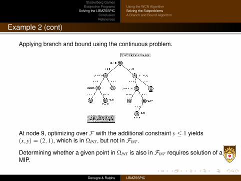
Example 2 (cont)

Applying branch and bound using the continuous problem.

At node 9, optimizing over F with the additional constraint y ≤ 1 yields(x, y) = (2, 1), which is in ΩINT , but not in FINT .

Determining whether a given point in ΩINT is also in FINT requires solution of aMIP.





Obtaining Lower Bounds

Instead of removing the integrality constraints, we can remove thefollower’s objective.

Doing so, we obtain the integer low-point problem, similar to thatsuggested in Moore and Bard [1990].

Integer Low-point Problem

min(x,y)∈ΩINT

f (x, y) (11)

The low-point problem is a true relaxation and produces a valid bound,since FINT ⊆ ΩINT .

If (11) is infeasible, then so is the original problem.





Obtaining Upper Bounds

Although OPT(F ) is not a valid lower bound, optimizing over F may stillbe a useful exercise.

If (x, y) is a solution to OPT(F ) and x ∈ XINT , we can solve the(unrestricted) follower’s problem with x fixed to x.

The resulting solution (if there is one) must then be in FINT .

In fact, we may want to optimize over F with the additional requirementthat x ∈ XINT .





Branching

The only way to verify optimality of a solution is when it is a low-pointsolution and also a member of FINT

Otherwise, we have no verifiable optimality conditions.

This means we may have to branch, even when all variables are integer.

This is only necessary for the leader’s variables.

There are many ways of performing such integer branching.

We will cover the details in the case of the LBMZSSPIC below.





Basic Branch and Bound Algorithm

The following is the loop for processing a node in the branch-and-boundalgorithm for solving a mixed-integer linear bilevel program.

Processing a Node

1 Solve the low-point problem (11) to obtain (x, y).1 If infeasible, fathom.2 If feasible and the bound exceeds the value of the incumbent, fathom.

2 Optimize over F (optionally requiring x ∈ XINT ) to obtain (x, y).3 If x ∈ XINT , solve the follower’s problem with x = x and update the

incumbent if possible.4 If all leader variables are fixed, then fathom.5 Otherwise, branch.

This is similar to the scheme proposed by Moore and Bard [1990].





Optimizing over F

Comment

In the continuous BLP, the follower’s problem is an LP, so we canreplace the optimality constraint with KKT conditions.

Taking this approach yields a nonconvex NLP. Two main approaches havebeen taken to solve this problem:

1 Linearize complementary slackness constraints by introducing binaryvariables and solve the 0-1 program with a MIP solver [Fortuny-Amatand McCarl, 1981].

2 Relax the complementary slackness conditions and branch on KKTmultipliers, checking the complementary slackness conditions at eachiteration [Bard and Moore, 1990].

Currently, we take the first approach, which allows us to easily enforcex ∈ XINT .





Solver for the LBMZSSPIC

So far, we have focused on generating supported solutions of (5).

This requires solving a weighted sum subproblem with only boundconstraints on the leader’s variables.

The low-point problem is a MILP and can be solved using standardmethods.

We use the following integer branching rule:

Pair Branching

Let (x, y) be the solution obtained in Step 2 of the node processingloop.

Let i and j be the indices of two unfixed leader variables.Create three child nodes as follows

1 xi = 1− xi and xj = xj2 xi = xi and xj = 1− xj3 xi = 1− xi and xj = 1− xj





Implementation

The algorithm has been implemented using software available from theComputational Infrastructure for Operations Research (COIN-OR) repository.

COIN-OR Components Used

The Abstract Library for Parallel Search (ALPS) to perform thebranch and bound.

The COIN Branch and Cut (CBC) framework for solving the MILPs.

The COIN LP Solver (CLP) framework for solving the LPs arisingin the branch and cut.

The Cut Generation Library (CGL) for generating cutting planeswithin CBC.

The Open Solver Interface (OSI) for interfacing with CBC and CLP.

Please visit www.coin-or.org for information on obtaining thesecodes.





Illustrating the Tradeoff

From this example we can see how the solution evolves:

vmin [rx, dy]

subject to x ∈ 0, 1n

y ∈ argmax dy : Ay ≤ b

0 ≤ y ≤ 1 − x

y ∈ 0, 1n¯

where

r = (5, 5, 10, 3, 3, 6, 8, 9, 3, 7),

d = (11, 12, 13, 15, 15, 7, 12, 10, 19, 16),

A = (5, 6, 7, 8, 9, 2, 5, 7, 10, 9),

b = 40




n r range problems solved cpu(s)10 0.50 [1,300] 13 131.8410 0.50 [1,300] 13 188.7310 0.50 [1,300] 9 83.55

An example of the generated frontier:

pgflastimage




Future Directions

The following directions are planned for the near future:

Better methods for optimizing over F .

Better methods for finding heuristic interdiction plans.

Implementation of the WCN algorithm.

Parallel solution of subproblems and global solution procedure.Extensive testing of interdiction for various problem classes

Combinatorial ProblemsGeneric MILPs




References

J.F. Bard and J.T. Moore. A branch and bound algorithm for the bilevel programming problem. SIAM Journal onScientific and Statistical Computing, 11(2):281–292, 1990.

O. Ben-Ayed and C. Blair. Computational difficulties of bilevel linear programming. Operations Research, 38:556–560, 1990.

P. Calamai and L. Vincente. Generating quadratic bilevel programming problems. ACM Transactions onMathematical Software, 20:103–119, 1994.

J. Fortuny-Amat and B. McCarl. A representation and economic interpretation of a two-level programming problem.Journal of the Operations Research Society, 32:783–792, 1981.

A.M. Geoffrion. Proper efficiency and the theory of vector maximization. Journal of Mathematical Analysis andApplications, 22:618–630, 1968.

P. Hansen, B. Jaumard, and G. Savard. New branch-and-bound rules for linear bilevel programming. SIAM Journalon Scientific and Statistical Computing, 13(5):1194–1217, 1992.

R. Jeroslow. The polynomial hierarchy and a simple model for competitive analysis. Mathematical Programming, 32:146–164, 1985.

J.T. Moore and J.F. Bard. The mixed integer linear bilevel programming problem. Operations Research, 38(5):911–921, 1990.

T.K Ralphs, M.J. Saltzman, and M.M. Wiecek. An improved algorithm for biobjective integer programming and itsapplication to network routing problems. Technical Report 04T-004, Lehigh University Industrial and SystemsEngineering, 2004.


Documents

Multiobjective Mixed-Integer Stackelberg Gamescoral.ie.lehigh.edu/~ted/files/talks/LBMZSSPIC-EURO06.pdf · mixed-integer zero-sum static Stackelberg problem (MZSSP): MZSSP min x