Multiobjective Bayesian Optimization Algorithm for Combinatorial Problems: Theory and practice

Josef Schwarz -L�t 2þHQiãHN

Brno University of Technology

Faculty of Engineering and Computer Science Department of Computer Science and Engineering

CZ - 61��� %UQR� %RåHW�FKRYD �

Tel.: 420 5 41141210, fax: 41141270, e-mail: schwarz@dcse.fee.vutbr.cz, Tel.: 420 5 41141283, fax: 41141270, e-mail: ocenasek@dcse.fee.vutbr.cz

Abstract: This paper deals with the utilizing of the Bayesian optimization algorithm (BOA) for the multiobjective optimization of combinatorial problems. Three probabilistic models used in the Estimation Distribution Algorithms (EDA), such as UMDA, BMDA and BOA which allow to search effectively on the promising areas of the combinatorial search space are discussed. The main attention is focused on the incorporation of Pareto optimality concept into classical structure of the BOA algorithm. We have modified the standard algorithm BOA for one criterion optimization utilizing the known niching techniques to find the Pareto optimal set. The experiments are focused on tree classes of the combinatorial problems: artificial problem with known Pareto set, multiple 0/1 knapsack problem and the bisectioning of hypergraphs as well.

Key Words: Multiobjective optimization, Pareto and non Pareto algorithms, evolutionary algorithms, probabilistic model, estimation distribution algorithms, Bayesian optimization algorithm, niching techniques.

1 Introduction

Combinatorial optimization problems such as placement problem, number partitioning problem (NPP), decomposition problem, traveling salesman problem (TSP), job-shop scheduling, bin packing problem, facility layout problem, knapsack problem, etc. belong to the class of NP hard problems [1]. The search space is often very large and it is not possible to use enumerative techniques because the complexity of the problems is expressed by O(n!) or O(rn), where n is the size of the problem and r<n is cardinality of used alphabet. To avoid the problem with finite alphabet string it is possible to replace the original string by kn bit string where k=log(r). In case r=2 the problem is reduced to binary optmization problem with 2n complexity. Let us note that we will focus on this type of encoding. Generally, the solution can be represented by a vector of parameters with unknown inter-parameter dependencies. However, many combinatorial optimization algorithms have no mechanism for capturing inter-parameter dependencies. But only this approach allows to concentrate the sampling more effectively on regions of the search space which have appeared to be promising in the past. Most optimization algorithms do this only by searching around the location of the best previous solution or by using various type of genetic algorithms (GA). The classical genetic algorithms (GA) have the common disadvantage - the necessity of the setting the parameters like crossover, mutation and selection rate and the choice of suitable type of genetic operators. That is why we have analysed and used some of the Estimation of Distribution Algorithms (EDAs) called probabilistic model-building genetic algorithms, too. The crossover and mutation operators used in standard GA are replaced in EDAs by probability estimation and sampling techniques. In case of probabilistic methods, statistics about the search space is explicitly maintained by creating models of the good solutions found. The efficiency of such techniques depends naturally on the complexity of model used and on the complexity of problems. Next we will discuss population based evolutionary algorithms using probabilistic models with various complexity. Let us denote:

D = (X1, X2,..,XN) with Xj ∈ D, is the population of the solutions/string/individuals X = (X0, X1,..,Xn-1) is a string/individual of length n with Xi as a variable x = (x0, x1,..,xn-1) is a string/individual with xi as a possible instantiation of variable Xi, xi ∈ {0,1} P = (p(x0), p(x1),..,p(xn-1)), with p(xi) ∈ [0,1 ] is the vector of univariate marginal probabilities p(x0 , x1,.. xn-1) = p(X0=x0 ,X1 =x1 ,..,Xn-1=xn-1) denotes the n dimensional distribution

2 Probabilistic models

The performance of EDA algorithms that work on the basis of probabilistic models can be specified on the following common framework:

Generate initial population of individuals of size M (randomly); While termination criteria is false do begin Select parent population of N individuals according to a selection method; Estimate the probability distribution of the selected parents; Generate new offspring according to the estimated probabilistic model; Replace some individuals in current population with generated offspring; end Next, we will describe three main types of probabilistic models used in EDA algorithms according to their complexity – model without inter-dependency, with pairwise dependencies and multivariate dependencies. 2.1 Models without dependencies

The probability vector P of univariate probabilities is used to model simple probability distribution. In Univariate Marginal Distribution Algorithm UMDA [2] it is assumed that variables are mutually independent, see Fig. 1a. For each variable position i∈ {0..n-1} and each possible value of this variable xi∈ {0,1}, the univariate marginal frequency pi (xi ) is defined as the frequency of strings that have xi on i-th position in the parent population D: 1[Q[S LLLL ���� = , where ni(xi) is a number of appearances of the allele xi on i-th

position. Each new individual X = (x0 ,x1,...,xn-1 ) is generated by UMDA according to the distribution:

∏−

==

�

�

����Q

LLL [S;S , (1)

so the value of i-th variable is set to value a with the probability equal to pi(a). UMDA is able to cover efficiently linear problems only. 2.2 Models with Pairwise dependencies

The univariate probability is used as in UMDA. In addition, the pair dependencies are allowed [3]. The bivariate marginal frequency pi,j(xi,xj) used in Bivariate Marginal Distribution Algorithm BMDA is defined as the frequency of individuals in parent population D, that have values xi and xj on positions i and j at the same time:

1[[Q[[S MLMLMLML ������ �� = . Conditional probability of occurrence of the value xi on i-th position in the case

of occurrence of xj on j-th position is determined �������_� �� MMMLMLMLML [S[[S[[S = (2)

We extended the concept of UMDA and BMDA for the alphabet encoding, so that xi∈ {0,…,ri-1} and xj∈ {0,…,rj-1} [4]. For each pair of positions i, j the count of each combination of values can be summarized into contingency table. Variable dependencies are discovered by Pearson’s chi-square statistics, we used in [4] the following form of equation:

∑ ∑ −=−

=

−

=

�LU

�N

�MU

�O M

�

�ML �

OQNLQ

ONQ1¸

ML�

����

����

�

� (3)

Variables are considered to be independent if the result does not meet certain threshold. For example binary

variables are independent for 95% if ���¸�ML �� < . The dependency information is used to build up the acyclic

dependency graph-probabilistic graphical model, which can be seen as a set of trees. Each new individual X = (x0 ,x1,...,xn-1 ) is generated according to the distribution

∏=−

=

�Q

�LLPL [;S [LS �_�� ��� (4)

where m(i) is any number between zero and n-1 or nothing (in case of root nodes of the tree). The root nodes correspond to the positions where the values are generated using the univariate marginal distribution, the values of positions connected to already generated positions in the graph are subsequently generated using the conditional probability. An example of the tree dependency graph is shown in Fig.1b.

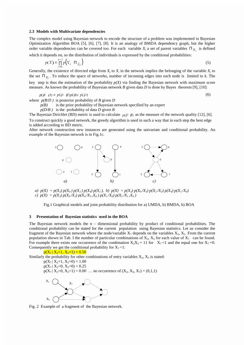
2.3 Models with Multivariate dependencies

The complex model using Bayesian network to encode the structure of a problem was implemented in Bayesian Optimization Algorithm BOA [5], [6], [7], [8]. It is an analogy of BMDA dependency graph, but the higher order variable dependencies can be covered too. For each variable Xi a set of parent variables

iXΠ is defined

which it depends on, so the distribution of individuals is expressed by the conditional probabilities:

( )∏ Π=−

=

�Q

�LL;L;S;S _�� (5)

Generally, the existence of directed edge from Xj to Xi in the network implies the belonging of the variable Xj to the set

L;Π . To reduce the space of networks, number of incoming edges into each node is limited to k. The

key step is thus the estimation of the probability p(X) via finding the Bayesian network with maximum score measure. As known the probability of Bayesian network B given data D is done by Bayes theorem [9], [10]:

������_��_� 'S%S%'S'%S = (6)

where p(B/D ) is posterior probability of B given D p(B) is the prior probability of Bayesian network specified by an expert p(D/B ) is the probability of data D given B The Bayesian Dirichlet (BD) metric is used to calculate �_� %'S as the measure of the network quality [12], [6].

To construct quickly a good network, the greedy algorithm is used in such a way that in each step the best edge is added according to BD metric. After network construction new instances are generated using the univariate and conditional probability. An example of the Bayesian network is in Fig.1c.

2

0

1

4 3

2 2

0 0

4

11

4 3 3 3

a) b) c) a) p(X) = p(X3) p(X0 ) p(X2 ) p(X4) p(X1 ), b) p(X) = p(X3) p(X0 /X3) p(X2 /X3) p(X4) p(X1 /X4) c) p(X) = p(X3) p(X0 /X3) p(X4 /X3 ,X0 ) p(X1 /X0) p(X2 /X1 ,X0 )

Fig.1 Graphical models and joint probability distribution for a) UMDA, b) BMDA, b) BOA

3 Presentation of Bayesian statistics used in the BOA

The Bayesian network models the n – dimensional probability by product of conditional probabilities. The conditional probability can be stated for the current population using Bayesian statistics. Let us consider the fragment of the Bayesian network where the node/variable X7 depends on the variables X2, X5. From the current population shown in Tab. I the number of particular combinations of X2, X5 for each value of X7 can be found. For example there exists one occurrence of the combination X2X5 = 11 for X7 =1 and the equal one for X7 =0. Consequently we get the conditional probability for X7 =1:

p(X7 | X2=1, X5=1) = 0.50 Similarly the probability for other combinations of entry variables X2, X5 is stated:

p(X7 | X2=1, X5=0) = 1.00 p(X7 | X2=0, X5=0) = 0.25

p(X7 | X2=0, X5=1) = 0.00 … no occurrence of (X2, X5, X7) = (0,1,1)

X2 X7

X5

Fig. 2 Example of a fragment of the Bayesian network.

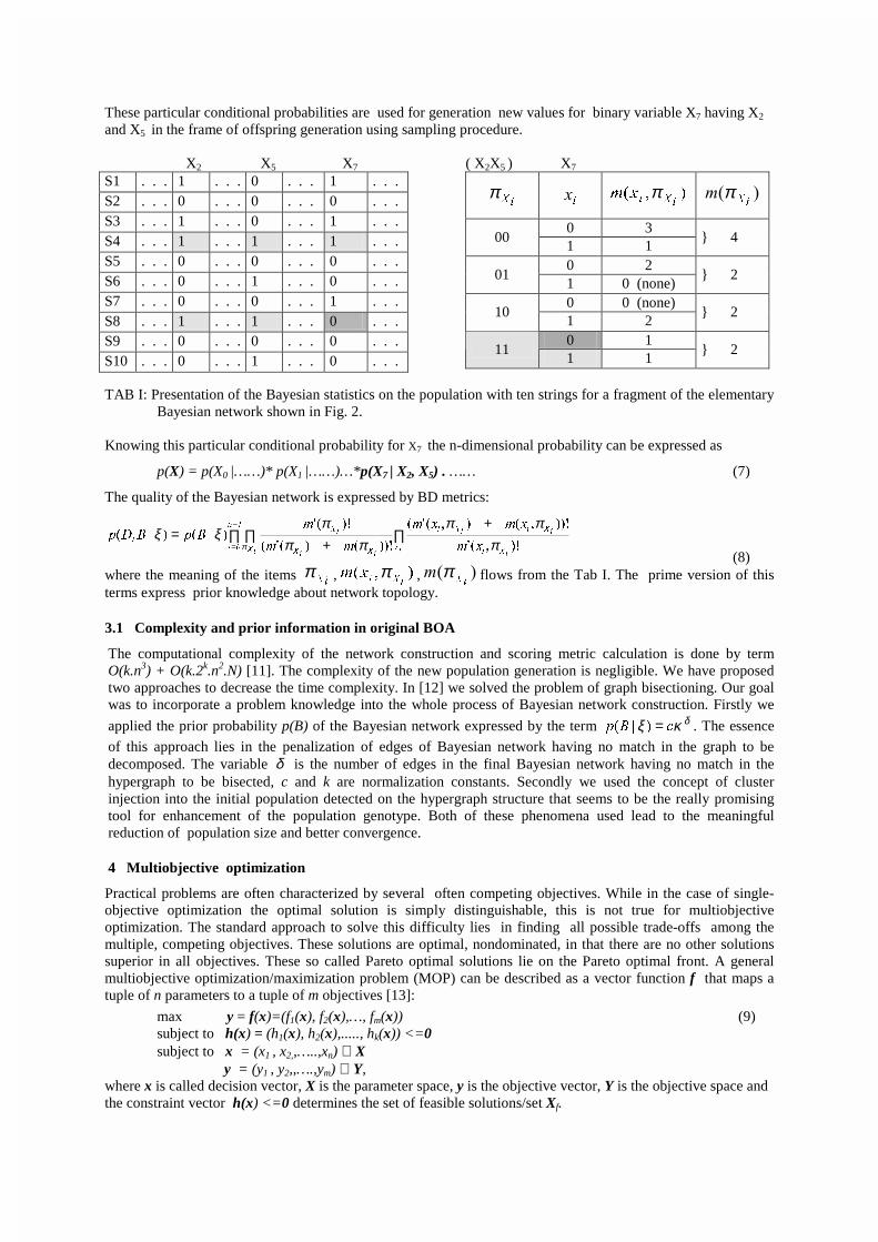
These particular conditional probabilities are used for generation new values for binary variable X7 having X2 and X5 in the frame of offspring generation using sampling procedure. X2 X5 X7

S1 . . . 1 . . . 0 . . . 1 . . . S2 . . . 0 . . . 0 . . . 0 . . . S3 . . . 1 . . . 0 . . . 1 . . . S4 . . . 1 . . . 1 . . . 1 . . . S5 . . . 0 . . . 0 . . . 0 . . . S6 . . . 0 . . . 1 . . . 0 . . . S7 . . . 0 . . . 0 . . . 1 . . . S8 . . . 1 . . . 1 . . . 0 . . . S9 . . . 0 . . . 0 . . . 0 . . . S10 . . . 0 . . . 1 . . . 0 . . .

( X2X5 ) X7

L;π L

� ���L;L

[P π ��L;

� π

0 3 00

1 1 } 4

0 2 01

1 0 (none) } 2

0 0 (none) 10

1 2 } 2

0 1 11

1 1 } 2

TAB I: Presentation of the Bayesian statistics on the population with ten strings for a fragment of the elementary

Bayesian network shown in Fig. 2. Knowing this particular conditional probability for X7 the n-dimensional probability can be expressed as

p(X) = p(X0 |……)* p(X1 |……)…*p(X7 | X2, X5) . …… (7)

The quality of the Bayesian network is expressed by BD metrics:

∏+

∏ ∏+

=−

= L[L;L

L;LL;L�Q

�LL;

L;L;

L;

[P

[P[P

PP

P%S%'S

����

���������

�������

����_��_��

πππ

πππ

ξξπ

(8)

where the meaning of the items L;

π , ���L;L

[P π , ��L;

� π flows from the Tab I. The prime version of this terms express prior knowledge about network topology. 3.1 Complexity and prior information in original BOA

The computational complexity of the network construction and scoring metric calculation is done by term O(k.n3) + O(k.2k.n2.N) [11]. The complexity of the new population generation is negligible. We have proposed two approaches to decrease the time complexity. In [12] we solved the problem of graph bisectioning. Our goal was to incorporate a problem knowledge into the whole process of Bayesian network construction. Firstly we

applied the prior probability p(B) of the Bayesian network expressed by the term δκξ F%S =�_� . The essence

of this approach lies in the penalization of edges of Bayesian network having no match in the graph to be decomposed. The variable δ is the number of edges in the final Bayesian network having no match in the hypergraph to be bisected, c and k are normalization constants. Secondly we used the concept of cluster injection into the initial population detected on the hypergraph structure that seems to be the really promising tool for enhancement of the population genotype. Both of these phenomena used lead to the meaningful reduction of population size and better convergence.

4 Multiobjective optimization

Practical problems are often characterized by several often competing objectives. While in the case of single-objective optimization the optimal solution is simply distinguishable, this is not true for multiobjective optimization. The standard approach to solve this difficulty lies in finding all possible trade-offs among the multiple, competing objectives. These solutions are optimal, nondominated, in that there are no other solutions superior in all objectives. These so called Pareto optimal solutions lie on the Pareto optimal front. A general multiobjective optimization/maximization problem (MOP) can be described as a vector function f that maps a tuple of n parameters to a tuple of m objectives [13]:

max y = f(x)=(f1(x), f2(x),…, fm(x)) (9) subject to h(x) = (h1(x), h2(x),....., hk(x)) <=0 subject to x = (x1 , x2,,…..,xn) ∈ X

y = (y1 , y2,,….,ym) ∈ Y, where x is called decision vector, X is the parameter space, y is the objective vector, Y is the objective space and the constraint vector h(x) <=0 determines the set of feasible solutions/set Xf.

The set of solutions of MOP includes all decision vectors for which the corresponding objective vectors cannot be improved in any dimension without degradation in another - these vectors are called Pareto optimal set. The idea of Pareto optimality is based on the Pareto dominance. For any two decision vectors u, v it holds

u v (u dominates v) iff f(u)>f(v), u = v (u weakly dominates v) iff f(u)>=f(v),

u ~ v (u is indifferent to v) iff u, v are not comparable

A decision vector u dominates decision vector v ( u v) iff fi(u ) ≥ fi(v) for i=1,2,.., m with fi(u )> fi(v) for at least one i. The vector u is called Pareto optimal if there is no vector v which dominates vector u in parameter space X. In objective space the set of nondominated solutions lies on a surface known as Pareto optimal front. The goal of the optimization is to find a representative sampling of solutions along the Pareto optimal front. An example of the concept of Pareto dominance and Pareto-optimal front are presented in a graphical form in Fig.3.

U

T

V

P

S

R

Pareto optimal front

Feasible region

f1

f2

U

T

V

P

S

R

f1

V dominates

V is dominated

indifferent

indifferent

f2

Fig. 3 Example of Pareto front and Pareto dominance.

It can be stated that solution V dominates solution S and T, solution V is dominated by U, solution U is nondominated and Pareto optimal, solution S is dominated by V and T.

5 Optimization methods

5.1 Pareto methods There are many papers that present various approaches to find Pareto optimal front almost based on the classical evolutionary algorithms. All of them must solve the problem of adequate solutions evaluation and population diversity. It was developed Pareto-based fitness assignment using the concept of dominance in order to determine the reproduction probability of each solution. It is evident that unlike the case of single optimization, fitness is related to the whole population. The multiobjective optimization is typical multimodal search for finding multiple different solutions in a single run. To reach this goal various niching techniques are used. The well known is fitness sharing – the more individuals are located in the neighborhood (defined by niche radius) of a solution the more is the fitness decreased. Less frequently nonniching techniques are used such as restricted mating (only similar parents are mated) and crowding (offspring replace similar parents). We will shortly mention the main representatives of the Pareto optimization algorithms: The Niched Pareto Genetic Algorithm (NPGA) combines tournament selection and the concept of Pareto dominance [14]. A wide review of basic approaches and the specification of original Pareto evolutionary algorithms include the dissertations [15], [13] where the last one describes the original Strength Pareto Evolutionary Algorithm (SPEA). An interesting approach using nondominated sorting in genetic algorithm (NSGA) is published in [16]. An interesting extension of the SPEA algorithm resulting in PESA algorithm is described in [17]. Pareto optimal methods have more preferences than disadvantages. To the advantages belongs the fact that Pareto approaches take all objectives into consideration simultaneously - every point/solution of Pareto front is good solution – and maintains the diversity of solutions. Naturally we can list two main disadvantages – this approach is computationally expensive and not very intuitive if the number of objectives is large. All these algorithms mentioned above progress towards the Pareto optimal set with a good distribution of solutions but none of them guarantees the convergence to true Pareto optimal set. The promising approach of archive-based Pareto optimization algorithms is published in [18] where the concept of ε-approximate Pareto set and ε-Pareto

set is introduced. A class of algorithms is suggested with guaranteeing convergence to a diverse set of ε-Pareto optimal solutions.

5.2 Non-Pareto methods

There are many methods for the multi-criteria optimization, mostly based on the scalarization of the objective function or other non-Pareto approaches. This way the MOP problem can be easily transformed into more simpler SOP problem.

Weighted - sum approach The well known aggregation method is based on the weighted sum approach. This method transforms the objective function vector into a higher scalar function using weighted sum of particular objectives. Let us note that in the single objective optimization, the feasible set is completely ordered according the single objective function. For two solutions u, v ε Xf either f(u)>=f(v) or f(v)>=f(u). In case of multiobjective optimization, the feasible set is only partially ordered. In case of maximization we get:

maximize y = f(x) = w1 f1(x)+ w2 f2(x) +.....+ wm fm(x) (10)

This equation can be modified to the following form which can be understand as a sector equation of line with the slope -w1/w2 and intercept y/w2 [13] (see Fig. 4.) :

f2 (x)=(-w1/w2) f1(x) + y/w2 (11)

f1

f2

slope -w1/w2 U

V

C

y/w2

f1

f2

U

V W

Feasible region

Infeasible region

c’

c

a) b) Fig. 4 Example of an exploration of the search space by a) weighted sum approach, b) constrained methods The set of parallel lines represents the successive search in the objective space. This approach is able to find Pareto optimal solutions but the search process is very sensitive to weight coefficients and this technique is not able to reach solutions in local non-convex region, see point C. Constraint method

This technique is quite simple: only one function is optimized, the others are transformed into constraints. Then the penalty function can be used to fulfil the constraints. For the case of bi-objective optimization we get

y = f1(x) (12) h(x)= f2(x)>= c,

where c is chosen repeatedly (see fig 4.b) but remark that the c’ is not available choice of bound. Another principle is used in priority (lexicographic) method - the objective with highest priority is minimized first, then the next with lower priority etc. The problem appears how to state the importance of objectives. Fuzzy- control approach

Fuzzy controllers are often used in control system and generally in soft computing. In [19] an interesting approach for scalarization of a bi-objective problem. Each generation the centre of current population is detected and according this knowledge fuzzy controller decides what transformation of the cost components into one-dimensional fitness function is taken.

Let us note that the attraction of the SOP methods described above is supported by many useful and well-studied heuristic methods like dynamic programming, branch and bound method, random search algorithm, stochastic local search algorithms and simulated annealing. In common they required several runs to obtain an approximation of the Pareto-optimal set.

6 Pareto optimal BOA

In our Pareto BOA algorithm we replaced the original fitness assignment and replacement step of standard BOA by the Pareto niching technique utilizing a new strength criterion for the evaluation process [13]. The following specification describes the whole reproduction process of our algorithm. Let us note that although we solved bi-objective optimization, our algorithm is able to solve m-objective optimization problems. The flowchart of our

Pareto BOA algorithm is in Fig. 5.

It follows from the flowchart that the algorithm is archive-oriented. In external archive the nondominated solutions during all optimization history are archived and enter regularly into selection and replacement phase. The most important part of our Pareto algorithm [20], [21] is the procedure for detection of nondominated (current Pareto front) and dominated solutions and sophisticated fitness calculation. The procedure for current nondominated and dominated set detection is described in following steps:

1. For each individual X in the population D compute the vector of the objective functions

������������� ;I;I;I;IP��

�= (13)

2. Detect subset of nondominated solutions { }MLLMM ;;';';;' �_ ∈∃∧∈= (14)

3. For each nondominated solution Xj from D compute its strength value as

{ }�'

;;';;;V

LMLL

M +

∧∈=

_��

(15)

4. The fitness for nondominated solutions is equal to the reverse of the strength value

���� MM ;V�;I =′ (16)

5. For each dominated solution Xi from D determine the fitness as

+=′ ∑

M;ML ;V��;I ���� , (17)

where LMM ;;'; ∧∈ .

Fig. 5 The flowchart of the Pareto BOA algorithm

7 Problem specification

7.1 Bi-objective Onemax/Xor binary problem

We start to test our algorithm with an artificial problem with easily determined Pareto optimal front. We call this problem Onemax/Xor problem (unitation versus pairs in [16]). It is defined on the binary string. Onemax function f2 is simply stated by number of ones in the n bit string X, e.g. f2(X)=f2(0110)=4. Xor function denoted as f1 is specified by number of pairs of adjacent complementary bits, either 10 or 01, thus f1(X)=f1(0110)=1+0+1=2. The goal is to maximize both functions. 7.2 Multiple 0/1 knapsack problem

Generally, the 0/1 knapsack problem consists of set of items, weight and profit associated with each item, and an upper bound of the capacity of the knapsack. The task is to find a subset of items which maximizes the sum

Population (t - 1) Archive (t - 1)

Truncate selection

Model construction

Sampling

Offspring (t)

Strength fitness computation

Pareto identification

Worst - case Pareto replacement elitism

Population (t) Archive (t)

Pareto set (t)

of the profits in the subset, yet all selected items fit into the knapsack so as the total weight does not exceed the given capacity. This single objective problem can be extended to multiobjective multiple problem by allowing more than one knapsack. Formally, the multiobjective 0/1 knapsack problem is defined in the following way: Given a set of n items and a set of m knapsacks, with following parameters:

MLS � profit of item j according to knapsack i

MLZ � weight of item j according to knapsack i

ci capacity of knapsack i

find a vector x = (x1, x2 ,....., xn) ∈ {0,1}n, such that xj =1 iff item j is selected and

f(x)=(f1(x), f2(x),…, fm(x)) is maximum, where (18)

fi(x) = ∑=

Q

�MMML [S � (19)

and for which the constraint is fulfilled

{ } ����� PL �∈∀ L

Q

�MMML F[Z �∑

=≤ (20)

The complexity of the problem solved depends on the values of knapsack capacity. According to [13] we used the knapsack capacities stated by the equation:

ci = 0.5 ∑=

Q

�MMLZ � (21)

The encoding of solution into chromosome is realized by binary string of the length n. To satisfy the constraints (21) it is necessary to use repair mechanism on the generated offspring to be feasible one.

7.3 Hypergraph bisectioning

The bisectioning problem can be defined as follows: Let us assume a hypergraph H=(V,E), with n =|V| nodes and e = |E| edges. We look for such a bisection (V1,V2) of V that minimizes the number of hyperedges that have nodes in different set V1, V2 and the balance b of the partition sizes. The set of external hyperedges can be labelled as Ecut (V1,V2). The cost function is the number of external hyperedges, shortly called cut size. Each solution of the bisection is encoded as a binary string X=(x0, x2, …, xn-1 ). The variable xi represents the partition number, the index specifies the node in the hypepergraph. For the case of simple graph G(V,E,R) bisectioning we have derived on the binary string X=(x0 , x1 ,.., xn-1) the following two functions to be minimized [18]:

���� ML

�Q

LM�L

MLLMFXW� [[�[[U��9�9(I ∑ −+==−

>=

(22)

f2 = b =| ∑ −−∑−

=

−

=

�Q

�L

L

�Q

�L

L [�[ �� | (23)

where the coefficient rij=1 in case the net/edge of the graph G exists between node i and j, else rij=0. The function f1 represents the cut value of the bisection and the function f2 expresses the balance/difference of the partition sizes. We have tested two approaches for solving this 2-objective optimization problems: Weighted sum approach and Pareto optimal method. The first approach transforms the original vector-valued objective function into a scalar-valued objective function. The objective function of the solution X is computed as a weighted sum of all objective functions:

f(X) = w1 f1(X)+ w2 f2(X), (24)

where w1, w2 are weight coefficients. It is well known the sensitivity of the optimization process to these values. We have tested two sets of these coefficients. In WSO1 variant we have chosen w1=0.5, w2=0.5, in WSO2 couple of w1=0.005, w2=0.995 was used. This values were found experimentally.

8 Experimental results

8.1 Test benchmarks

We used three types of benchmarks:

1. The 64 bit Onemax/Xor function with known Pareto set including 32 indifferent solution.

2. Two knapsack benchmarks specified by 100 (Kn100) and 250 items (Kn250) published on the web site [http://www.tik.ee.ethz.ch/~zitzler/testdata.html#fileformat]. We have compared our results with results

obtained by two evolutionary algorithms SPEA [13] and NSGA[16]. These two algorithms represent well working evolutionary multiobjective algorithms.

3. Two hypergraph IC67, IC116 representing real circuits. The global optima is not known. The structure of circuits can be characterized as a random logic. The hypergraph IC67 consists of 67 nodes and 134 edges/nets, the IC116 consists of 116 nodes and 329 edges/nets.

8.2 Experiments and results All experiments were run on Sun Enterprise 450 machine (4 CPUs, 4 GB RAM), in the future we consider the utilizing the cluster of Sun Ultra 5 workstations.

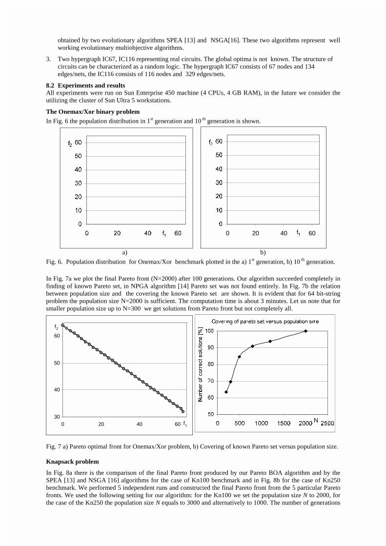
The Onemax/Xor binary problem

In Fig. 6 the population distribution in 1st generation and 10 th generation is shown.

�

��

��

��

��

��

��

� �� �� ��I�

I�

�

��

��

��

��

��

��

0 20 40 60I�

I�

a) b)

Fig. 6. Population distribution for Onemax/Xor benchmark plotted in the a) 1st generation, b) 10 th generation.

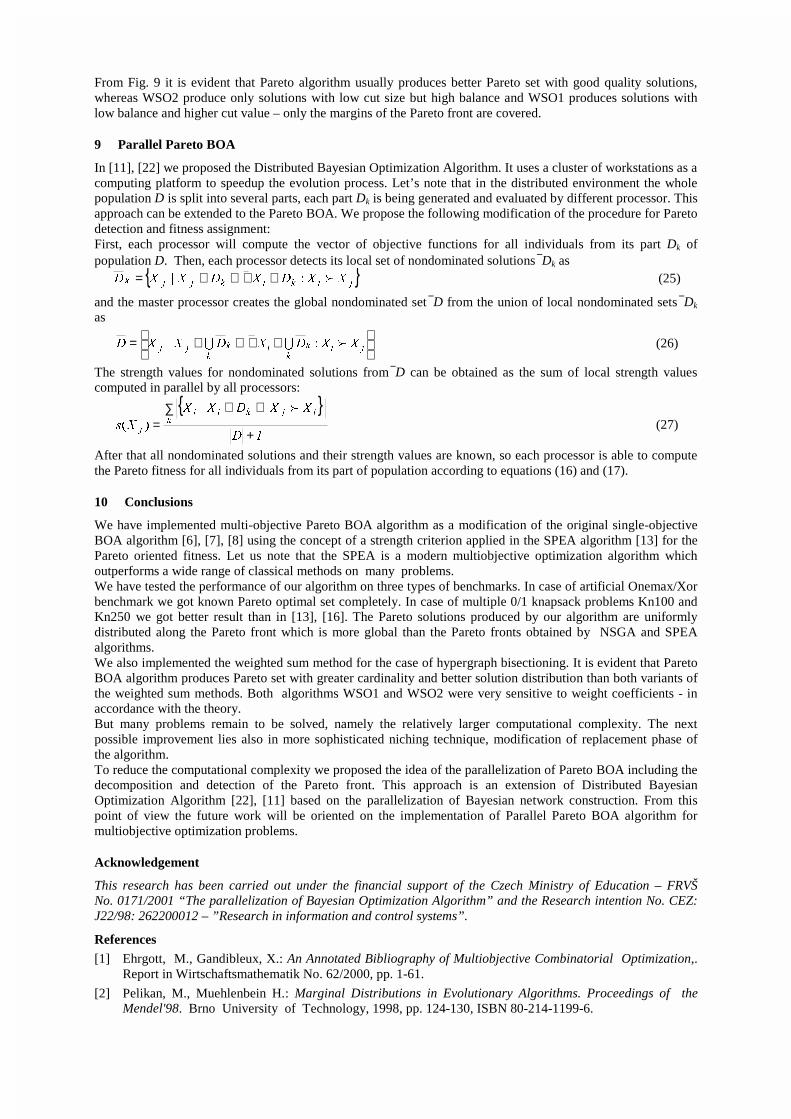
In Fig. 7a we plot the final Pareto front (N=2000) after 100 generations. Our algorithm succeeded completely in finding of known Pareto set, in NPGA algorithm [14] Pareto set was not found entirely. In Fig. 7b the relation between population size and the covering the known Pareto set are shown. It is evident that for 64 bit-string problem the population size N=2000 is sufficient. The computation time is about 3 minutes. Let us note that for smaller population size up to N=300 we get solutions from Pareto front but not completely all.

30

40

50

60

0 20 40 60 f 1

f 2 &RYHULQJ RI SDUHWR VHW YHUVXV SRSXODWLRQ VL]H

��

��

��

��

��

���

� ��� ���� ���� ���� ����1

1XPEHURIFRUUHFWVROXWLR

QV>�

@

Fig. 7 a) Pareto optimal front for Onemax/Xor problem, b) Covering of known Pareto set versus population size. Knapsack problem

In Fig. 8a there is the comparison of the final Pareto front produced by our Pareto BOA algorithm and by the SPEA [13] and NSGA [16] algorithms for the case of Kn100 benchmark and in Fig. 8b for the case of Kn250 benchmark. We performed 5 independent runs and constructed the final Pareto front from the 5 particular Pareto fronts. We used the following setting for our algorithm: for the Kn100 we set the population size N to 2000, for the case of the Kn250 the population size N equals to 3000 and alternatively to 1000. The number of generations

used is 150. The computation time is presented in Tab II. In the context of algorithm comparison an important question arises: What measure should be used to express the quality of the results so that the various evolutionary algorithms can be compared in a meaningful way. We preferred the topology/shape of the Pareto fronts in our comparison. From a it is evident that for Kn100 the Pareto solutions produced by our Pareto BOA in the middle part of Pareto front are slightly better than the Pareto solutions produced by SPEA and NSGA. What is more important – our Pareto BOA produces more solutions in the Pareto front margins.

����

����

����

����

����

����

����

����

����

����

���� ���� ���� ���� ���� ����I�

I� 16*$

63($

%2$

����

����

����

����

����

����

����

����

����

����

����

�����

���� ���� ���� ���� ���� I�

I�

16*$

63($

%2$ 1 ����

%2$ 1 ����

Fig. 8 Comparison of final Pareto fronts for a) Kn100, N=2000, b) Kn250, N=3000 and N=1000.

In Fig. 8b we see that for Kn250 the difference between Pareto fronts is more expressive – our Pareto BOA for N=3000 outperforms the SPEA and NSGA. In case of limited size N=1000 the Pareto BOA is slightly worse than SPEA, but the Pareto front is longer.

Problem size n Population size N, Number of generations Computational time Kn100 N=1000, 150 gen. 2 min 40 s Kn100 N=2000, 150 gen. 5 min Kn250 N=1000, 150 gen. 25 min Kn250 N=3000, 150 gen. 45 min

TAB. II Computational time for knapsack problems Hypergraph bisectioning

The five independent runs of each algorithm were performed and final Pareto front from final populations is shown. For better visualization of the fronts from each run the points are connected by lines.

��

��

��

��

��

��

� �� �� ��I�

I �IRU:62�

�

�

��

��

��

��

I �

:62 �

3DUHWR

:62 �

�

�

�

�

�

��

��

��

�� �� �� I�

I �

3DUHWR

:62 �

:62 �

Fig. 9a Bisection of IC67, N=2500. Fig. 9b Bisection of IC116, N=4000.

From Fig. 9 it is evident that Pareto algorithm usually produces better Pareto set with good quality solutions, whereas WSO2 produce only solutions with low cut size but high balance and WSO1 produces solutions with low balance and higher cut value – only the margins of the Pareto front are covered.

9 Parallel Pareto BOA

In [11], [22] we proposed the Distributed Bayesian Optimization Algorithm. It uses a cluster of workstations as a computing platform to speedup the evolution process. Let’s note that in the distributed environment the whole population D is split into several parts, each part Dk is being generated and evaluated by different processor. This approach can be extended to the Pareto BOA. We propose the following modification of the procedure for Pareto detection and fitness assignment: First, each processor will compute the vector of objective functions for all individuals from its part Dk of population D. Then, each processor detects its local set of nondominated solutions Dk as

{ }MLNLNMMN ;;';';;' �_ ∈∃∧∈= (25)

and the master processor creates the global nondominated set D from the union of local nondominated sets Dk as

∈∃∧∈= ML

N

NLN

NMM ;;';';;' �� �_ (26)

The strength values for nondominated solutions from D can be obtained as the sum of local strength values computed in parallel by all processors:

{ }�'

;;';;

;V NLMNLL

M +

∑ ∧∈=

_

��

(27)

After that all nondominated solutions and their strength values are known, so each processor is able to compute the Pareto fitness for all individuals from its part of population according to equations (16) and (17).

10 Conclusions

We have implemented multi-objective Pareto BOA algorithm as a modification of the original single-objective BOA algorithm [6], [7], [8] using the concept of a strength criterion applied in the SPEA algorithm [13] for the Pareto oriented fitness. Let us note that the SPEA is a modern multiobjective optimization algorithm which outperforms a wide range of classical methods on many problems. We have tested the performance of our algorithm on three types of benchmarks. In case of artificial Onemax/Xor benchmark we got known Pareto optimal set completely. In case of multiple 0/1 knapsack problems Kn100 and Kn250 we got better result than in [13], [16]. The Pareto solutions produced by our algorithm are uniformly distributed along the Pareto front which is more global than the Pareto fronts obtained by NSGA and SPEA algorithms. We also implemented the weighted sum method for the case of hypergraph bisectioning. It is evident that Pareto BOA algorithm produces Pareto set with greater cardinality and better solution distribution than both variants of the weighted sum methods. Both algorithms WSO1 and WSO2 were very sensitive to weight coefficients - in accordance with the theory. But many problems remain to be solved, namely the relatively larger computational complexity. The next possible improvement lies also in more sophisticated niching technique, modification of replacement phase of the algorithm. To reduce the computational complexity we proposed the idea of the parallelization of Pareto BOA including the decomposition and detection of the Pareto front. This approach is an extension of Distributed Bayesian Optimization Algorithm [22], [11] based on the parallelization of Bayesian network construction. From this point of view the future work will be oriented on the implementation of Parallel Pareto BOA algorithm for multiobjective optimization problems.

Acknowledgement

This research has been carried out under the financial support of the Czech Ministry of Education – FRVŠ No. 0171/2001 “The parallelization of Bayesian Optimization Algorithm” and the Research intention No. CEZ: J22/98: 262200012 – ”Research in information and control systems”.

References

[1] Ehrgott, M., Gandibleux, X.: An Annotated Bibliography of Multiobjective Combinatorial Optimization,. Report in Wirtschaftsmathematik No. 62/2000, pp. 1-61.

[2] Pelikan, M., Muehlenbein H.: Marginal Distributions in Evolutionary Algorithms. Proceedings of the Mendel'98. Brno University of Technology, 1998, pp. 124-130, ISBN 80-214-1199-6.

[3] Pelikan, M., Muehlenbein H.: The bivariate Marginal Distribution Algorithms. Advances of Soft Computing-Engineering Design and Manufacturing. London: Springer Verlag, p. 521-535.

[4] 6FKZDU]� -�� 2þHQiãHN� -�� Experimental Study: Hypergraph Partitioning Based on the Simple and Advanced Genetic Algorithm BMDA and BOA, Proceedings of the Mendel'99 Conference, Brno University of Technology, 1999, pp. 124-130, ISBN 80-214-1131-7.

[5] Baluja, S, Davies S.: Using Optimal Dependency-Trees for Combinatorial Optimization: Learning The Structure of the Search Space. Proc. 1997 International Conference on Machine Learning, pp.30-38.

[6] Pelikan, M.: A Simple Implementation of Bayesian Optimization Algorithm in C++(Version1.0). Illigal Report 99011, February 1999, pp. 1-16.

[7] Pelikan, M., Goldberg, D. E., & Cantú-Paz, E.: Linkage Problem, Distribution Estimation, and Bayesian Networks. IlliGal Report No. 98013, November 1998,pp. 1-25.

[8] Pelikan, M., Goldberg, D. E., & Lobo, F.: A Survey of Optimization by Building and Using Probabilistic Model, Illigal Report 99018, September 1999, pp. 1-12.

[9] Gottvald, A.: Bayesian Evolutionary optimization. Proceedings of the Mendel'99 Conference, Brno University of Technology, Faculty of Mechanical Engineering, Brno, 999, pp. 30-35, ISBN 80-214-1131-7.

[10] Etxeberria R., Larranaga, P.: Global Optimization using Bayesian networks. II. Symposium on Artificial Inteligence. CIMAF99. Special Session on Distributions and Evolutionary Optimization, 1999, 7 pages.

>��@ 2þHQiãHN� -�� 6FKZDU]� -�� The Parallel Bayesian Optimization Algorithm, Proceedings of the European Symposium on Computational Inteligence, Physica-Verlag, Košice, Slovak Republic, 2000, pp. 61-67, ISBN 3-7908-1322-2, ISSN 1615-3871.

>��@ 6FKZDU]� -�� 2þHQiãHN� -�� The knowledge-based evolutionary algorithm KBOA for hypergraph bisectioning. Proceedings of the Fourth Joint Conference on Knowledge-based Software Engineering Brno, Czech Republic, 2000, pp.51-58, ISBN 1 58603 060 4 (IOS Press).

[13] Zitzler, E.: Evolutionary Algorithms for Multiobjective Optimization: Methods and Applications PhD thesis, Swiss Federal Institute of Technology (ETH), Zurich, Switzerland, November 1999.

[14] Horn, J., Nafpliotis, N., Goldberg, D.E.: A Niched Pareto Genetic Algorithm for Multiobjective Optimization, In Proceedings of the First IEEE Conference on Evolutionary Computation, IEEE World Congress on Computational Intelligence, Vol. 1, pages 82-87, Piscataway, New Jersey, June 1994. IEEE Service Center.

[15] Coello, C. A.: An Empirical Study of Evolutionary Techniques for Multiobjective Optimization in Engineering Design. PhD thesis, Department of Computer Science, Tulane University, New Orleans, LA, April 1996.

[16] Srinivas, N., Deb, K.: Multiobjective Optimization using Nondominated Sorting in Genetic Algorithm. Evolutionary Computation, Vol.2, No. 3, 1994, pp. 221-248.

[17] Corne, D. W., et al.: The Pareto Envelope-based Selection Algorithm for Multiobjective optimization. Proceedings of the Sixth International Conference on Parallel Problem Solving from Nature (PPSN VI), pages 839-848, Berlin, September 2000. Springer.

[18] Laumanns, M., et al.: On the convergence and Diversity-Preservation Properties of Multi-Objective Evolutionary Algorithm. Swiss Federal Institute of Technology (ETH), Zurich, Switzerland, May 2001.

[19] Cvetkovic, D., Parmee, I.: Evolutionary Design and Multi-objective Optimization. EUFIT’98, September 7-10, 1998, ELITE Foundation, Aachen, Germany, pp.397-401.

>��@ 6FKZDU]� -�� 2þHQiãHN� -�� Evolutionary Multiobjective Bayesian Optimization Algorithm: Experimental Study, Proceedings of the 35th Spring International Conference MOSIS'01, Vol. 1, MARQ Ostrava, Hradec nad Moravicí, 2001, pp.. 101-108, ISBN 80-85988-57-7.

>��@ 6FKZDU]� -�� 2þHQiãHN� -�� Pareto Bayesian Optimization Algorithm for the Multiobjective 0/1 Knapsack Problem, Proceedings of the 7th International Mendel Conference on Soft Computing, Brno University of Technology, Faculty of Mechanical Engineering, Brno, 2001, s. 131-136, ISBN 80-214-1894-X.

[22] 2þHQiãHN� -�� 6FKZDU]� -�� The Distributed Bayesian Optimization Algorithm for Combinatorial Optimization, EUROGEN 2001 - Evolutionary Methods for Design, Optimization and Control with Applications to Industrial Problems, Athens, Greece, September 19-21st, 2001, accepted paper.