Multimaterial topology optimization · alternating active-phase algorithm for multimaterial topology optimization problems a 115-line matlab implementation r. tavakoli and s.m. mohseni

ALTERNATING ACTIVE-PHASE ALGORITHM FOR

MULTIMATERIAL TOPOLOGY OPTIMIZATION PROBLEMS

A 115-LINE MATLAB IMPLEMENTATION

R. TAVAKOLI AND S.M. MOHSENI

Abstract. A new algorithm for the solution of multimaterial topology opti-

mization problems is introduced in the present study. The presented method

is based on the splitting of a multiphase topology optimization problem intoa series of binary phase topology optimization sub-problems which are solved

partially, in a sequential manner, using a traditional binary phase topology

optimization solver; internal solver. The coupling between these incompletesolutions is ensured using an outer iteration strategy based on the block coordi-

nate descend method. The presented algorithm provides a general framework

to extend the traditional binary phase topology optimization solvers for thesolution of multiphase topology optimization problems. The overall algorith-

mic complexity of the presented algorithm is independent of the number of

desired phases, p, and its computational cost is approximately proportional top2. The interesting features of the presented algorithm are: generality, simplic-

ity, efficiency, ease of implementation and the inheritance of the convergenceproperties of its internal optimization solver. The presented algorithm is used

to solve multimaterial minimum structural and thermal compliance topology

optimization problems based on the classical optimality criteria method. Thedetails of MATLAB implementation are presented and the complete program

listings are provided as the supplementary materials. The success and perfor-

mance of the presented method are demonstrated through several two dimen-sional numerical examples.

Keywords. Coordinate descent method; MATLAB code; Multi-

phase topology optimization; Optimality criteria.

Contents

1. Introduction 22. Statement of multiphase topology optimization problem at abstract level 43. Statement of alternating active phase algorithm at abstract level 64. Comment on the convergence theory of alternating active phase algorithm 105. Model problems 105.1. Minimum compliance topology optimization problem 105.2. Minimum thermal compliance topology optimization problem 116. MATLAB implementation of model problems 117. Numerical results and discussion 157.1. Minimum compliance topology optimization 157.2. Minimum thermal compliance topology optimization 28

Date: April 15, 2013.R. Tavakoli (corresponding author: [email protected], faculty member), S.M. Mohseni (un-

dergraduate student), Materials Science and Engineering Department, Sharif University of Tech-nology, Tehran, Iran, P.O. Box 11365-9466, Tel: 982166165209, Fax: 982166005717.

1

mailto:[email protected]

2 R. TAVAKOLI AND S.M. MOHSENI

7.3. Grid resolution study 317.4. Sensitivity to the maximum inner iterations (iter max in) 317.5. Sensitivity to the filter radius 328. Summary 34References 34Supplement A. 115-line MATLAB code for multimaterials minimum compliance

topology optimization 36Supplement B. 115-line MATLAB code for multimaterials minimum thermal

compliance topology optimization 38

1. Introduction

A topology optimization problem is to determine the unknown material(s) dis-tribution within a pre-defined spatial domain, such that some optimality conditionshold. After the seminal paper by Bendsøe and Kikuchi [1], the structural topologyoptimization (c.f. [2, 3]) has been received significant attention within the com-putational mechanics and civil engineering communities. It is currently known asa standard method for design of engineering structures at micro and macro scalesunder simple and complex service conditions. An interesting question in this con-text is that whether it is possible to use multiple materials under volume or weightconstraint to find a better design in terms of the structure’s performance and/ormanufacturing cost. This is particularly attractive in the case of multiphysics prob-lems and/or multifunctional structures. However, the majority of researches in thisfield are limited to binary-phase (materials-void) topology optimization problems.To the best of our knowledge there are a few works focused on the solution ofmultiphase topology optimization problems. In the remainder of this section theliterature of multimaterial topology optimization will be reviewed briefly and thenthe original contribution of the current study will be outlined.

From a physical point of view, the most important aspect of a multimaterialstopology optimization problem is the representation of the material properties ten-sors as a function of local volume fractions and physical properties of individualphases. It is commonly performed using material interpolation [4], homogenization[3, 5] or averaged Hashin-Shtrikman (HS) upper-lower bounds [3] approaches.

Using the homogenization method, design of three-phase composites with ex-tremal thermal expansion, piezoelectricity and bulk modulus are considered in [6, 7],[8] and [9] respectively (cf. [10]). These design problems have been formulated assome three-phase topology optimization problems. In these works authors howeverdid not attend to numerical solution of resulted systems of optimality conditions andpassed it to a general purpose optimization black-box. In addition to these works,there are some works in which the authors paid specific attention to introduce spe-cial numerical methods to solve multiphase topology optimization problems. Priorto reviewing these works, it is worth to mention that difficulties aroused from thenumerical solution of multiphase topology optimization problems. These difficultiesare mainly related to the mathematical structure of design space. In the case oftwo-phase topology optimization, the design variable is a field variable that includesthe local volume fraction of one of the contributing phases. The correspondingdesign space is commonly a sufficiently regular field with local lower and upperbounds, and a global integral constraint. This structure makes it possible to keep

MULTIMATERIAL TOPOLOGY OPTIMIZATION 3

the solution strictly feasible with respect to optimization constraints; for instanceusing the optimality criteria [3] or gradient projection [11] methods. However, inthe case of multiphase topology optimization problems not only there are multiplefield variables (related to volume fractions of different phases), their correspondinglower and upper bounds and multiple global integral constraints but also there arepointwise constraints on summation of volume fraction fields (the incompressibilityconstraint). The later constraints significantly increases the computational cost ofthe corresponding numerical solution.

To decrease the complexity of design domain, a phase-field approach coupled toa special materials interpolation method has been used in [12, 13] to solve three-phase topology optimization problems. In this method one field variable has beenused to determine the volume fraction of different phases. Although it still suffersfrom the existence of multiple global constraints, the mentioned local constraints(computationally expensive constraints) are naturally removed using mono-field de-sign variable. However because of using mono-field materials interpolation method,it permits only the existence of at most two phases within each computational cellsimultaneously, i.e., triple junctions are mandatory filtered by this approach.

The variational multilevel sets approach (cf. [14, 15]) has been adapted in [16–18] to solve multimaterials topology optimization problems. Later, the piecewise-constant variational level set method (cf. [17]) has been used in [19, 20] to improvethe computational cost of former approach. Some of drawbacks of level-set basedmethods are: the mesh dependency of convergence speed (due to CFL stabilitycondition) and dependency of final topology to initial design. Moreover, the globalvolume constraints are only satisfied at final solutions.

Using multimaterial phase-field approach based on Cahn-Hilliard equation, ageneral method to solve multiphase structural topology optimization problems havebeen introduced in [21, 22]. The intrinsic volume preserving property is the mostimportant benefit of this method, i.e., the iterations will be kept strictly feasiblewith respect to design domain without any further effort. The slow convergence ofthe phase field method is however the main difficulty of this approach. For instanceover 104 iterations are commonly required to find a suitable topology. This limita-tion stems in severe time-step restriction due to the stability of the correspondingforth order parabolic PDEs for evolution of phase-field variables. Moreover, dueto the existence of an interfacial penalization in Cahn-Hilliard energy functional,i.e., penalizes the total area of interfaces, the resulted topologies are always bi-ased to topologies with minimal interfaces and curvatures. It is worth mentioningthat for binary phase composites under periodic boundary conditions rank-N lam-ination is known to be the optimal microstructure, while due to large interfacialarea such solutions are discouraged by phase-field approach. This undesirable ef-fect also appears in variational level set based approaches, as they similarly includean interfacial penalization term due to regularization of level set functions. An-other difficulty with phase field approach is existence of many phenomenologicalconstants in the model that should be carefully selected to find desired solutions.

For the sake of completeness it is worth to mention that the extension of evo-lutionary topology optimization methods [23] to manage multiple materials is an-other candidate to solve multiphase topology optimization problems. In [24] abi-directional evolutionary topology optimization method has been suggested tosolve multiphase structural topology optimization problems.


In the present work a new multimaterials topology optimization method basedon the block coordinate descent approach will be introduced. The main propertiesof the presented method are: generality, simplicity, efficiency and the ease of im-plementation. An interesting feature of our approach is that it provides a generalframework to convert almost every binary phase topology optimization solver toits multiphase counterpart by a few modifications; without special regard to thenature of related topology optimization problem. Moreover, this work goals to be atutorial for computer implementation of the presented approach. For this purposethe MATLAB implementation of our approach to solve some model problems willbe discussed in details.

2. Statement of multiphase topology optimization problem atabstract level

The statement of a typical multiphase topology optimization problem will bepresented in this section. Because the algorithm, presented in the next section, issufficiently general, the presentation here will be kept at an abstract level, to utilizeits application to a wide class of topology optimization problems.

Consider Ω as the design domain. It is assumed that Ω is a fixed nonemptyand sufficiently regular subset of Rd (d = 1, 2, 3). In an multimaterial topologyoptimization problem the goal is to find the optimal distribution of p ∈ N (p > 2)number of distinct materials inside Ω. Possibly, the void could be considered as aseparate phase in our formulation. Therefore, the binary phase topology optimiza-tion problem here implies the classical void-material topology optimization prob-lem. The materials distribution is determined by the local volume fraction fields,αi (i = 1, . . . , p), corresponding to the contributing phases (note that αi = αi(x)).It is assumed that αi ∈ V(Ω), where V is a sufficiently regular function space (inmany practical topology optimization problems L∞ is the minimal regularity re-quirement). Obviously we have the following pointwise bound constraints on everyαi,

li 6 αi 6 ui, i = 1, . . . , p (1)

where 0 6 li 6 ui 6 1 and the inequalities are understood componentwise here. Itis worth to mention that to fix the topology of a material at a specific portion ofΩ, it is suffice to use the desired fixed value instead of lower and upper bounds in1. Since no overlap and gap are allowed in the desired design, the summation ofvolume fractions at every point x ∈ Ω should be equal to unity, i.e.,

p∑i=1

αi = 1 (2)

where the summation operator is understood componentwise (local) here. In manytopology optimization problems we usually have one global volume constraint onthe total volume of each material inside Ω, i.e.,∫

Ω

αi dx = Λi|Ω|, i = 1, . . . , p (3)

where Λi are user defined parameters; obviously 0 6 Λi 6 1 and∑pi=1 Λi = 1.

These constraints are commonly called as resource constraints. Without loss ofgenerality, we restrict ourselves to equality resource constraints in this study. Con-sidering 2, it is possible to remove volume fraction field of one material and solve


the problem for p − 1 unknown topology indicator fields. This way is frequent inbinary phase topology optimization problems. However, applying this reductionhas no benefit in the present study.

For the purpose of convenience we condense all design vectors (scalar fields)into a single vector field denoted by α, i.e., α = α1, . . . , αp. Since we solve afinite-dimensional version of original problem in practice, we use superscript h inthis study to denote the (finite dimensional) vector corresponding to each topologyfield. Therefore, after space discretization, the admissible design space, A, couldbe defined as follows:

Ah :=

αh ∈ αhi ∈ Vh(Ωh) i∈1,...,p

∣∣∣∣∣∣∑pi=1 α

hi = 1,∫

Ωh αhi dx = Λi|Ωh|, i = 1, . . . , p

lhi 6 αhi 6 uhi , i = 1, . . . , p

When p = 2, the structure of simplex Ah is very simple and there are effi-

cient numerical methods to manage these constraints during optimization cycles,for instance using optimality criteria [3] or projected gradient [11] methods. How-ever, when p > 2 the structure of Ah is very complex and to our knowledge thereis no (time-linear) algorithm to manage these constraints. This is indeed one ofthe main difficulties against efficient solution of multiphase topology optimizationproblems. It is worth to mention that in Cahn-Hilliard method used in [22] theseconstraints are naturally manipulated without additional computational penalty.The presented approach in this study provides a very simple way to manage theseconstraints in expense of a computational complexity similar to that of the opti-mality criteria or the projected gradient approaches. In fact, our algorithm herehas a time-linear computational complexity to manage these constraints.

In every topology optimization problem, the local material properties are a lo-cal function of volume fractions of contributing phases. Depending on the typeof problem, the material properties could be the specific mass density, thermalconductivity, elasticity tensor, etc. Having materials properties as a function oflocal volume fractions is one of the most important ingredient of every topologyoptimization problem. There are many different methods to compute local mate-rials properties based on the local volume fractions, for instance: linear mixtureapproach, SIMP penalized mixture approach (cf. [3, 4]), averaged lower and upperHashin-Shtrikman bounds (cf. [4, 9, 25]) and homogenization approach (cf. [3, 5]).In the present study it is assumed that the functionality of local materials prop-erties are provided by user. To simplify expositions, this function will be denotedby M(α) in the present study. Note that we do not care whether there is a singlematerial property or multiple ones and simply use M(α) to denote the functionthat interpolates the materials properties from local volume fraction data.

A PDE or a system of PDE constraint(s) is another ingredient of every topologyoptimization problem. Based on the physics of problem the PDE could be tran-sient, static or hybrid. Without loss of generality we limit ourselves here to staticproblems. Assume that the solution of PDE constraint is denoted by U ∈ U(Ω),where U is a sufficiently regular function space. Obviously U is an implicit functionof α, i.e., U(x) = U(α(x)). Note that U could be a scalar field (e.g. in ther-mal problems), vector field (e.g. in elasticity problems) or combination of scalerand vector fields (e.g. in multiphysics problems like thermomechanical problems).The partial differential operator corresponding to PDE constraint(s) is denoted byoperator R(· · · ) in the present study. Therefore, the discretized version of PDE


constraint(s) could be expressed as follows:

Rh(M(αh), Uh(αh)

)= 0 in Ωh (4)

where Uh ∈ Uh(Ωh) and the corresponding boundary conditions are encapsulatedinto the discritized version of PDE operator.

Definition of the objective functional is the remaining part of the problem state-ment here. In general the objective functional, J (· · · ), is an integral over Ω whichdepends on α and U . The discretized form of objective functional is expressed inthe following form in this study:

minαhJ h(αh, Uh(αh)

)(5)

Considering above terminology, every multimaterial topology optimization prob-lem could be expressed in the following abstract from:

minαh∈Ah

J h(αh, Uh(αh)

)subject to : Rh

(M(αh), Uh(αh)

)= 0 in Ωh (6)

3. Statement of alternating active phase algorithm at abstractlevel

The statement of alternating active phase algorithm will be presented in thissection. Currently there are many scientific and commercial codes to solve binary-phase topology optimization problems based on different methods. However, ex-tension of these codes to solve multiphase topology optimization problems is not astraightforward procedure. In addition, by such an extension, algorithms may lossefficiency and robustness. The motivation for development of alternating activephase algorithm is to provide a general framework to convert binary phase topol-ogy optimization codes to multiphase ones by minimal efforts and modifications.Moreover, keeping the efficiency and robustness of original algorithms are anotherfactors considered in the present work. Because our algorithm is sufficiently gen-eral, the presentation here will be kept at an abstract level, to make it possible toapply this algorithm to different classes of topology optimization problems.

The alternating active phase algorithm includes an outer iteration in whichp(p − 1)/2 binary phase topology optimization subproblems are solved partially(i.e., incomplete solution), using an appropriate binary phase topology optimiza-tion solver. This procedure could be performed either independently (in parallel)or sequentially; similar to Jacobi and Gauss-Seidel iterations, respectively. Duringthe solution of every subproblem, the topologies of p − 2 phases are fixed to thelast known values and those of two remained phases (active phases) will be varied.If active phases are denoted by subscripts ”a” and ”b”, αhab is used to denote thedesign vector in which αha and αhb could be varied and αhi is fixed for i 6= a, b.

Therefore, an appropriate binary phase topology optimization solver is requiredin the alternating active phase algorithm. This solver is called as the internal op-timization solver, henceforth. Roughly speaking, it is easy to make the internaloptimization solver by modification of binary phase topology optimization algo-rithm. The first required modification is to replace the binary phase materialsproperties operator M(·) with its corresponding multiphase counterpart, M(αhab).

In the binary phase topology optimization algorithms, the admissible designspace, Ahbi, has a simple structure. If the local volume fraction of stiff phase is


denoted by field vector wh, Ahbi could be expressed as follows:

Ahbi :=wh ∈ Vh(Ωh)

∣∣ lh 6 wh 6 uh,

∫Ωh

wh dx = Λ |Ωh|

In practice the lower and upper bounds lh and uh are set near 0h and 1h respec-tively. Because the topologies of p − 2 phases are fixed during every binary phasetopology optimization step in our algorithm, the second required modification isto modify the structure of Ahbi. Assuming the topologies of p − 2 phases are fixedinside Ωh, the remained volume fraction field, denoted by rhab, which could be var-ied during every binary phase topology optimization sub-problem is computed asfollows:

rhab = 1h −p∑

i=1i6=a,b

αhi (7)

Since∑pi=1 αi = 1 within each computational cell, it is only required to take the

volume fraction of a as the design variable of the binary phase topology optimizationsub-problem. After solving this sub-problem, the volume fraction field of phase b(background phase) could be computed by the following relation:

αhb = rhab − αha (8)

Considering 7, the corresponding (temporary) upper bound to phase a, uha,temp,during the binary phase topology optimization sub-problem should be computedas follows (note that lower bound does not need any modification):

uha,temp = min (uha , rhab) (9)

Theretofore, the admissible design space corresponding to the binary phase topologyoptimization sub-problem in which the topologies of phases a and b will be varied,Ahab, could be expressed as follows (phase b is assumed to be the background phase):

Ahab :=αha ∈ Vh(Ωh)

∣∣ lha 6 αha 6 uha,temp,

∫Ωh

αha dx = Λa |Ωh|

Therefore the internal optimization solver, denoted by operator Sh(αhab,M, Uh,Rh),should solve the following binary topology optimization problem:

minαh

ab∈Ahab

J h(αhab, U

h(αhab))

s.t. : Rh(M(αhab), U

h(αhab))

= 0 in Ωh (10)

Because of nonlinear nature of topology optimization problems, the internaloptimization solver uses an iterative procedure. Therefore, it needs a convergenceand/or termination criteria. The infinity norm, ‖ · ‖∞, of change in design vectorduring two consecutive optimization cycles is commonly used as the terminationcriterion. In the other word, when the maximum of local change in the topologyis smaller than a user defined threshold, the iterations are discarded, and the lastdesign vector is reported as an approximate optimal solution. Moreover, one maydefine an upper bound on the number of optimization cycles (posing limitationon the computational cost) as a stopping criterion. Input parameters ”tol in”and ”iter max in” are defined as the stopping criteria for internal optimizationalgorithm in the present study.

To avoid checkerboard instability and/or length scale control (cf. [26]), a filtering(smoothing) mechanism is commonly used in binary phase topology optimizationproblems. The filter parameters have a significant effect on the convergence rate


and resulted topologies of the internal optimization solver. The selection of filter pa-rameters is more serious in numerical solution of multiphase topology optimizationproblems. According to our numerical experience (will be mentioned later), dy-namic change in filter parameters leads to a more efficient and robust optimizationalgorithm. The filter parameters are denoted by ”filter params” in the presentstudy.

Prior to the presentation of alternating active phase algorithm, we will madesome elementary assumptions on the properties of internal optimization solver.

Assumption 1. The internal optimization solver is globally convergent1.

Assumption 2. The internal optimization solver is interior with respect to PDEand design constraints. In the other word, iterations of the internal optimizationsolver will be strictly feasible with respect to all constraints.

As it is formerly mentioned, in the case of two phase topology optimizationproblems, the structure of admissible design domain is very simple such that itis possible to keep optimization iterations strictly feasible with respect to Ah, inexpense of a negligible computational cost. Moreover, in most of topology optimiza-tion algorithms the corresponding PDE(s) is solved at every stage of optimization.Therefore, 2 is not a restrictive assumption.

In practical engineering design problems, we may not essentially look for a localsolution to the mathematical model corresponding to the physical problem, butsome improvements on an initial design could be of interest, or even sufficient. Inthis case, having a monotone interior algorithm could be suffice. Note that aninterior algorithm here does not imply an interior-point algorithm. For instance,the classical optimality criteria algorithm possesses requirements of assumption 2.The optimality criteria algorithm however is not globally convergent, except in somespecial cases. Therefore, we may relax assumption 1 to the following counterpart:

Assumption 3. The internal optimization solver is monotone with respect to theobjective functional. In the other word, the objective functional decreases monoton-ically as iterations of the internal optimization algorithm proceed.

Assuming phases are arranged from stiffer to softer as phase counter increasesfrom 1 to p, the Gauss-Seidel version of alternating active phase algorithm is pre-sented in algorithm 1. The Jacobi version of alternating active phase algorithmcould be expressed by some simple modifications in algorithm 1. The requiredmodifications are mentioned in algorithm 2 (to save the space, similar parts areremoved).

1An algorithm is globally convergent, if it converges to a local solution starting from an arbi-trary initial guess.


Algorithm 1: Alternating active phase algorithm (Gauss-Seidel version)

Problem definition:

given p, Ω, M, R, J , Λ1, . . . ,Λp, l1, . . . , lp, u1, . . . ,up1

Solution parameters:

given h, tol in, iter max in, filter params, tol out, iter max out2

Discretization:

compute Ωh, Rh, J h, lh1 , . . . , lhp, uh1 , . . . ,uhp3

Initialization:

αh1 , . . . , αhp = Λ1, . . . ,Λ1, iter out = 04

Outer iterations:

repeat5

αh,old = αh6

for a = 1 to p do7

for b = a + 1 to p do8

αhab = αh9

params in = tol in, iter max in, filter params10

αh = solution of Sh(αhab,M, Uh,Rh) with params in11

end12

end13

update filter params14

iter out = iter out + 115

change out = ‖αh − αh,old‖∞16

until (change out < tol out) and (iter out < iter max out) ;17

Algorithm 2: Alternating active phase algorithm (Jacobi version)

· · ·1

repeat2

αh,old = αh, ζh = 03

for a = 1 to p do4

for b = a + 1 to p do5

params in = · · ·6

ζh = ζh+ solution of Sh(αhab,M, Uh,Rh) with params in7

end8

end9

αh = ζh/(p(p− 1)/2)10

· · ·11

until (· · · ) ;12


4. Comment on the convergence theory of alternating active phasealgorithm

In this section we briefly comment on the convergence theory of the alternatingactive phase algorithm. As it is mentioned in the previous section, having aninterior and monotone topology optimization algorithm is suffice for many practicaltopology optimization applications. The alternating active phase algorithm inheritsthis property from its internal optimization solver. Therefore the following corollaryis evident:

Corollary 4.1. Alternating active phase algorithm is monotonic and interior underassumptions 2 and 3.

To establish the global convergence theory of alternating active phase algorithm isa more delicate issue. We believe that such a theory should be developed based onthe detailed properties of the internal optimization solver.

It is worth to mention that the alternating active phase algorithm is in closeconnection to the cyclic coordinate descent method (c.f. [section 5.4.3 of 27] and[section 8.9 of 28]) which is an ancient optimization algorithm. More precisely thealternating active phase algorithm is similar to block-wise cyclic coordinate descentmethods. Although cyclic coordinate descent methods are very old and inefficientin general, they are revisited recently and significant contribution has been doneduring the past two decades. It is mainly because of their promising efficiency tosolve special classes of large scale real-world problems. There are many theoreticalworks on the convergence of cyclic coordinate descent methods which could be usedto establish the convergence theory of the alternating active phase algorithm, undersome specific conditions. Because our goal is not to do a theoretical study in thiswork, we end this section refereing interested readers to [27–33].

5. Model problems

5.1. Minimum compliance topology optimization problem. The volume con-strained (binary phase) minimum compliance topology optimization problem is oneof the most common model problem in the literature of topology optimization. Inthis model problem, the unknown materials distribution is determined such thatthe stiffness of structure is maximized. To avoid the trivial solution, a global vol-ume constraint is applied on the total volume occupied by the stiff phase in thefinal design. In this section we recall multi-phase version of this model problem.Our test problem here is similar to that of [22].

In the case of minimum compliance topology optimization problem, the materialsproperties operator M is analog to the elasticity tensor, C(x) = C(α(x)). Notethat C is a forth order supersymmetric tensor (symmetric in both the right andthe left Cartesian index pair, together with symmetry under the interchange of thepairs). Following [22], the SIMP modified version of linear interpolation is usedwithin our materials interpolation operator:

C(α) =

p∑i=1

αqi Ci (11)


where Ci is the constant stiffness tensor corresponding to phase i-th. For a givenmaterials distribution α, the PDE operator R could be expressed as follows:

∇ · (C : D(u)) = f(x) in Ωu(x) = u(x) on Γu

(C : D(u)) · n = 0 on Γf(C : D(u)) · n = t(x) on Γt

(12)

where u denotes the displacement field which is analog to the state variable U in ourformerly mentioned abstract formulation, f denotes the volumetric body force, udenotes the prescribed displacement on boundaries Γu, Γf denotes the traction free

part of boundaries, t denotes the traction of structure with environment throughtraction boundaries, Γt and ∂Ω = Γu∪Γf∪Γt. Moreover, D(u) := 1

2 (∇u+(∇u)T ) =12 (∂iuj + ∂jui)i,j , i, j = 1 . . . , d. Note that the double dot operator, :, denotesthe usual contraction over two sets of indices. The objective functional, to beminimized, is defined as follows for this test problem:

J (α,u) =1

2

∫Ω

(C(α) : D(u)) : D(u) dx (13)

To solve this problem, we use a gradient based minimization approach. There-fore, the gradient of the objective functional should be computed. It could betrivially computed using the classical adjoint approach (c.f. [2, 3]).

5.2. Minimum thermal compliance topology optimization problem. Mini-mum thermal compliance problem (c.f. [3]) is the scalar counterpart of the minimumcompliance topology optimization problem stated in section 5.1. In this case thematerials properties operator should be replaced by thermal conductivity tensor,K:

K(α) =

p∑i=1

αqi Ki (14)

where Ki is the conductivity tensor corresponding to phase i-th. For a given ma-terials distribution α, the PDE operator R could be expressed as follows: ∇ · (K(α) ∇u) = f(x) in Ω

u(x) = u(x) on Γu(K ∇u) · n = q(x) on Γq

(15)

where u denotes the temperature field which is analog to the state variable Uin our abstract formulation, f denotes the thermal heat source, u denotes theprescribed temperature on boundaries Γu, q denotes the prescribed heat flux on Γqand ∂Ω = Γu ∪ Γq. The corresponding objective functional is defined as follows:

J (α, u) =1

2

∫Ω

K ∇u · ∇u dx (16)

6. MATLAB implementation of model problems

A 99-line MATLAB code has been introduced in [34] to solve minimum compli-ance topology optimization problems. Later, in [35] the size of Sigmund’s 99-lineMATLAB code has been reduced to 88 lines and its performance has considerablybeen improved by Sigmund and his co-workers. In this section, we shall commenton the list of major modifications required to modify the 88-line MATLAB code to


solve multiphase minimum compliance topology optimization problems. Becauseour goal here is to introduce the utility of the alternating phase framework, we willnot care on the performance of our code. It is tried to keep names of parametersand variables in the code consistent to those of presented algorithm. Therefore,to save the space, the parameters and variables will not essentially be defined ex-plicitly in this section (interested readers are recommended to consult [35]). Thecomplete listing of MATLAB code is included in the supplement A of this paper.

The main function, to call multimaterial topology optimization module, has thefollowing structure:

1 function main

2 [nx,ny,tol_out,tol_f,iter_max_in,iter_max_out,p,q,e,v,rf] = set_parameters ();

3 multi_top(nx,ny,tol_out,tol_f,iter_max_in,iter_max_out,p,q,e,v,rf);

4 end

where set parameters function defines the optimization parameters and mesh res-olution, and function multitop does the multimaterial topology optimization pro-cedure. e and v include the elasticity and volume fraction parameters of all phasesrespectively (analog to E0 and volfrac in 88-line MATLAB code). Moreover, rfand tol f denote the filter radius and filter adjusting tolerance; will be describedlater. In fact filter params ≡ rf, tol f. A typical form of set parameters

function is as follows (these parameters are related to cantilever beam #1 test casedescribed in section 7.1):

5 function [nx,ny,tol,tolf,im_in,im_out,p,q,e,v,rf] = set_parameters()

6 nx = 96; ny = 48; tol = 0.001; tolf = 0.05; im_in = 2; im_out = 200;

7 p = 3; q = 3; e = [2 1 1e-9]’; v = [0.4 0.2 0.4]’; rf = 8;

8 end

Following Algorithm 1, the MATLAB implementation of multi top function couldbe expressed as follows:

9 function multi_top(nx,ny,tol_out,tol_f,iter_max_in,iter_max_out,p,q,e,v,rf)

10 alpha = zeros(nx*ny,p);

11 for i = 1:p

12 alpha(:,i) = v(i);

13 end

14 % MAKE FILTER

15 [H,Hs] = make_filter (nx,ny,rf);

16 change_out = 2*tol_out; iter_out = 0;

17 while (iter_out < iter_max_out) && (change_out > tol_out)

18 alpha_old = alpha;

19 for a = 1:p

20 for b = a+1:p

21 [obj,alpha] = bi_top(a,b,nx,ny,p,v,e,q,alpha,H,Hs,iter_max_in);

22 end

23 end

24 iter_out = iter_out + 1;

25 change_out = norm(alpha(:)-alpha_old(:),inf);

26 fprintf(’Iter:%5i Obj.:%11.4f change:%10.8f\n’,iter_out,obj,change_out);

27 % UPDATE FILTER

28 if (change_out < tol_f) && (rf>3)

29 tol_f = 0.99*tol_f; rf = 0.99*rf; [H,Hs] = make_filter (nx,ny,rf);


30 end

31 % SCREEN OUT TEMPORAL TOPOLOGY

32 I = make_bitmap (p,nx,ny,alpha);

33 image(I), axis image off, drawnow;

34 end

35 end

In the above code function make filter does the sensitivity filtering to avoid thetopological instability during the optimization procedure. It is identical to that of88-line MATLAB code. It is based on a single path of discrete Laplacian smootherwith compact support of radius rf. It is worth to mention that other filters (e.g.PDE filter based on Helmholtz equation) presented in [35] led us to similar results,therefore, no attention will be paid here in regard to the selection of filter type.

36 function [H,Hs] = make_filter (nx,ny,rmin)

37 ir = ceil(rmin)-1;

38 iH = ones(nx*ny*(2*ir+1)^2,1);

39 jH = ones(size(iH));

40 sH = zeros(size(iH));

41 k = 0;

42 for i1 = 1:nx

43 for j1 = 1:ny

44 e1 = (i1-1)*ny+j1;

45 for i2 = max(i1-ir,1):min(i1+ir,nx)

46 for j2 = max(j1-ir,1):min(j1+ir,ny)

47 e2 = (i2-1)*ny+j2; k = k+1; iH(k) = e1; jH(k) = e2;

48 sH(k) = max(0,rmin-sqrt((i1-i2)^2+(j1-j2)^2));

49 end

50 end

51 end

52 end

53 H = sparse(iH,jH,sH); Hs = sum(H,2);

54 end

Our numerical experiments in the present work have shown that the selection offilter radius is a key success of the optimization procedure. According to our experi-ments, the dynamic modification of this parameter is required to bypass undesirablelocal minimums. Staring from a sufficiently large rf and decreasing it graduallyleads to a robust optimization procedure. To exploit this issue in our algorithm,we decrease rf (by factor 0.99 in this work) whenever change out < tol f, asimplemented in the above code. Moreover, to avoid the topological instability (cf.[26]) a strict lower bound is considered for parameter rf in our implementation(rf > 3 in this work).

Unlike the binary phase topology optimization, the visualization of resultedtopology is not a straightforward task. It is because we have multiple volumefraction fields, should be illustrated in a single plot. To do this, the functionmake bitmap is designated in this work to generate an appropriate bitmap imagefrom multi-field volume fraction data. The MATLAB implementation of this func-tion is as follows (although its algorithm is general, we restrict our code to fivephases in this study):

55 function I = make_bitmap (p,nx,ny,alpha)


56 color = [1 0 0; 0 0 .45; 0 1 0; 0 0 0; 1 1 1];

57 I = zeros(nx*ny,3);

58 for j = 1:p

59 I(:,1:3) = I(:,1:3) + alpha(:,j)*color(j,1:3);

60 end

61 I = imresize(reshape(I,ny,nx,3),10,’bilinear’);

62 end

Matrix color is a p× 3 matrix include desired RGB colors corresponding to desiredcolors for phase 1 : p; the row i-th of color includes the desired color of phase i-th.

Function bi top is the modified binary phase topology optimization function,i.e., modified version of top88 in [35].

63 function [o,alpha] = bi_top(a,b,nx,ny,p,v,e,q,alpha_old,H,Hs,iter_max_in)

64 alpha = alpha_old; iter_in = 0; nu = 0.3;

65 %% PREPARE FINITE ELEMENT ANALYSIS

66 A11 = [12 3 -6 -3; 3 12 3 0; -6 3 12 -3; -3 0 -3 12];

67 A12 = [-6 -3 0 3; -3 -6 -3 -6; 0 -3 -6 3; 3 -6 3 -6];

68 B11 = [-4 3 -2 9; 3 -4 -9 4; -2 -9 -4 -3; 9 4 -3 -4];

69 B12 = [ 2 -3 4 -9; -3 2 9 -2; 4 9 2 3; -9 -2 3 2];

70 KE = 1/(1-nu^2)/24*([A11 A12;A12’ A11]+nu*[B11 B12;B12’ B11]);

71 nodenrs = reshape(1:(1+nx)*(1+ny),1+ny,1+nx);

72 edofVec = reshape(2*nodenrs(1:end-1,1:end-1)+1,nx*ny,1);

73 edofMat = repmat(edofVec,1,8)+repmat([0 1 2*ny+[2 3 0 1] -2 -1],nx*ny,1);

74 iK = reshape(kron(edofMat,ones(8,1))’,64*nx*ny,1);

75 jK = reshape(kron(edofMat,ones(1,8))’,64*nx*ny,1);

76 %% DEFINE LOADS AND SUPPORTS (CANTILEVER BEAM)

77 F = sparse(2*(ny+1)*(nx+1),1,-1,2*(ny+1)*(nx+1),1);

78 fixeddofs = [1:2*ny+1];

79 U = zeros(2*(ny+1)*(nx+1),1);

80 alldofs = [1:2*(ny+1)*(nx+1)];

81 freedofs = setdiff(alldofs,fixeddofs);

82 %% INNER ITERATIONS

83 while iter_in < iter_max_in

84 iter_in = iter_in + 1;

85 %% FE-ANALYSIS

86 E = e(1)*alpha(:,1).^q;

87 for phase = 2:p

88 E = E + e(phase)*alpha(:,phase).^q;

89 end

90 sK = reshape(KE(:)*E(:)’,64*nx*ny,1);

91 K = sparse(iK,jK,sK); K = (K+K’)/2;

92 U(freedofs) = K(freedofs,freedofs)\F(freedofs);

93 %% OBJECTIVE FUNCTION AND SENSITIVITY ANALYSIS

94 ce = sum((U(edofMat)*KE).*U(edofMat),2);

95 o = sum(sum(E.*ce));

96 dc = -(q*(e(a)-e(b))*alpha(:,a).^(q-1)).*ce;

97 %% FILTERING OF SENSITIVITIES

98 dc = H*(alpha(:,a).*dc)./Hs./max(1e-3,alpha(:,a)); dc = min(dc,0);

99 %% UPDATE LOWER AND UPPER BOUNDS OF DESIGN VARIABLES

100 move = 0.2;

101 r = ones(nx*ny,1);

102 for k = 1:p

103 if (k ~= a) && (k ~= b)

104 r = r - alpha(:,k);

105 end


106 end

107 l = max(0,alpha(:,a)-move);

108 u = min(r,alpha(:,a)+move);

109 %% OPTIMALITY CRITERIA UPDATE OF DESIGN VARIABLES

110 l1 = 0; l2 = 1e9;

111 while (l2-l1)/(l1+l2) > 1e-3

112 lmid = 0.5*(l2+l1);

113 alpha_a = max(l,min(u,alpha(:,a).*sqrt(-dc./lmid)));

114 if sum(alpha_a) > nx*ny*v(a); l1 = lmid; else l2 = lmid; end

115 end

116 alpha(:,a) = alpha_a;

117 alpha(:,b) = r-alpha_a;

118 end

119 end

Comparing function bi top and top88, the list of required modifications in top88

are evident.Therefore, by adding about 30 lines of code and doing a little modifications on

top88 code, we can solve multiphase topology optimization problem based on [35]approach. In the same manner, it should not be difficult to apply the alternatingactive phase framework to other binary phase topology optimization problems.

To illustrate the utility of above mentioned modification to similar problem withdifferent physics, we did the implementation of our algorithm for solution of mini-mum thermal compliance topology optimization problems. For this purpose, 91-lineMATLAB code presented in section 5.1.6 of [3] for minimum thermal compliancetopology optimization problem was firstly modified according to 88-line MATLABcode of [35] recipes (to improve the computational performance). Then, the al-ternating active phase framework has been applied to it. The complete listing ofmultiphase version of minimum thermal compliance topology optimization solveris included in supplement B of this paper.

7. Numerical results and discussion

The success and performance of the alternating active phase algorithm will bestudied in this section by means of numerical experiments. A personal computerwith an AMD 2.4 GHz and 2.5 GB DDR2 RAM is used as the computationalresource in this study.

7.1. Minimum compliance topology optimization. The numerical results cor-responding to the model problem mentioned in section 5.1 are presented in this sec-tion. For this purpose, three minimum compliance topology optimization problemswhich are frequently used in the literature are considered here. They are cantileverbeam, bridge structure and MBB beam; as shown in figure 1. The load F whichis shown in figure 1 is equal to unity in all of our test cases here. To compareour results to available literature, the geometries and boundary conditions of thesetest cases are selected similar to those of [22]. To save the computational cost, thesymmetry of computational domain and loads is considered in bridge structure andMBB beam test cases (note that the presented results are however related to fulldomain in these cases).


F

?

Cantilever Beam

F2F

F

?

Bridge Structure

F

?

MBB Beam

Figure 1. Geometries and boundary conditions corresponding tominimum compliance model problems (unspecified boundary con-dition denotes the traction free boundary condition).

The optimization control parameters, to be set in set parameters function inall of test cases in this section are as follows:

function [...] = set_parameters ()

...

tol_out = 0.001; tol_f = .05; iter_max_in = 2; iter_max_out = 200; q = 3; rf = 8;

...

end

Note that we did not pay any specific attention to adjust these parameters in our nu-merical experiments here. Note that the careful selection of these parameters couldimprove the computational performance and outcome of our algorithm. The otherdesign optimization parameters corresponding to these test problems are listed intable 1 (these parameters are adapted from [22]).

Table 1. Design parameters of minimum compliance topology op-timization test cases.

Test Problem nx ny p e v

Cantilever Beam #1 96 48 3 [2 1 1e − 9]′ [0.4 0.2 0.4]′

Cantilever Beam #2 96 48 4 [4 2 1 1e − 9]′ [0.2 0.1 0.1 0.6]′

Bridge Structure #1 96 96 3 [2 1 1e − 9]′ [0.35 0.25 0.4]′

Bridge Structure #2 96 96 3 [2 1 1e − 9]′ [0.4 0.2 0.4]′

Bridge Structure #3 96 96 4 [9 3 1 1e − 9]′ [0.2 0.1 0.1 0.6]′

MBB − Beam #1 96 48 3 [2 1 1e − 9]′ [0.4 0.2 0.4]′

MBB − Beam #2 96 48 4 [4 2 1 1e − 9]′ [0.2 0.15 0.15 0.5]′

MBB − Beam #3 96 48 4 [9 3 1 1e − 9]′ [0.16 0.08 0.08 0.68]′


The MATLAB implementation of boundary conditions corresponding to can-tilever beam case is identical to lines 77 and 78 of the MATLAB code presented insection 6. For the other two cases, they should be replaced by:

...

%% DEFINE LOADS AND SUPPORTS (HALF OF MBB-BEAM)

F = sparse(2,1,-1,2*(ny+1)*(nx+1),1);

fixeddofs = union([1:2:2*(ny+1)],[2*(nx+1)*(ny+1)]);

...

...

%% DEFINE LOADS AND SUPPORTS (HALF OF BRIDGE STRUCTURE)

F = sparse([2*(ny+1) 2*(ny+1)*(nx/2+1)],[1 1],[-2 -1] ,2*(ny+1)*(nx+1),1);

fixeddofs = union([1:2:2*(ny+1)],[2*(nx+1)*(ny+1)]);

...

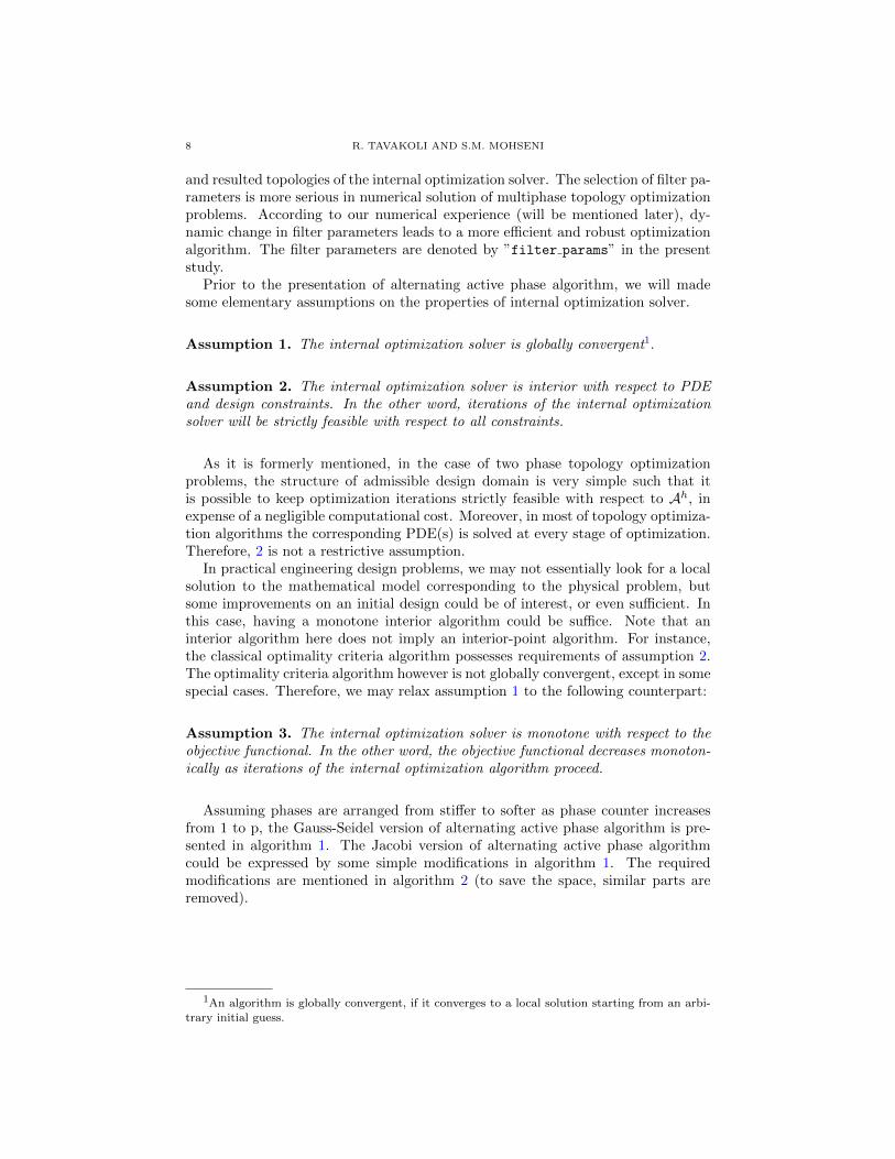
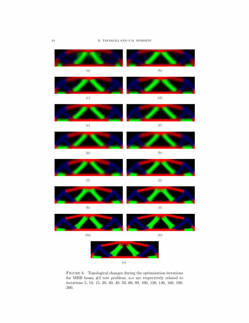
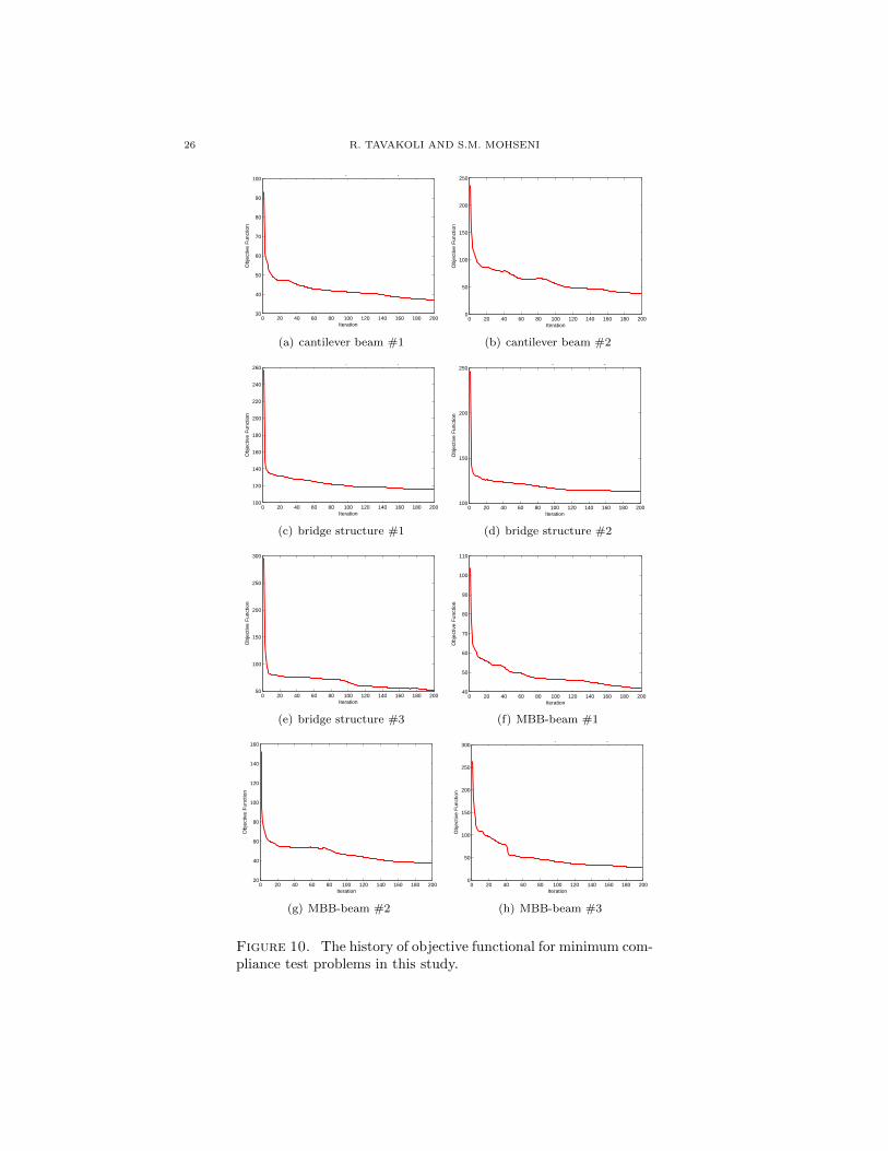
The topological evolution during optimization cycles corresponding to the afore-mentioned test problems, are shown in figures 2 to 9. Each plot includes 15 frameswhich are respectively related to (outer) iterations: 5, 10, 15, 20, 30, 40, 50, 60,80, 100, 120, 140, 160, 180, 200. The coloring scheme is adapted from [22], i.e., thehardness of phases is decreased based on the following order: red, blue, green andblack. The history of objective function during the optimization iterations (outeriterations) is plotted in figure 10. Figure 11 compares our results to those of [22].The consumed CPU time corresponding to these experiments are listed in table 2.

Table 2. Minimum compliance topology optimization test cases:CPU times in second.

Cantilever#1 Cantilever#2 Bridge#1 Bridge#2 Bridge#3 MBB#1 MBB#2 MBB#3

521 1435 1165 1174 1789 641 920 914


(a) (b) (c)

(d) (e) (f)

(g) (h) (i)

(j) (k) (l)

(m) (n) (o)

Figure 2. Topological changes during the optimization iterationsfor cantilever beam #1 test problem; a-o are respectively relatedto iterations 5, 10, 15, 20, 30, 40, 50, 60, 80, 100, 120, 140, 160,180, 200.


(a) (b) (c)

(d) (e) (f)

(g) (h) (i)

(j) (k) (l)

(m) (n) (o)

Figure 3. Topological changes during the optimization iterationsfor cantilever beam #2 test problem; a-o are respectively relatedto iterations 5, 10, 15, 20, 30, 40, 50, 60, 80, 100, 120, 140, 160,180, 200.


(a) (b) (c)

(d) (e) (f)

(g) (h) (i)

(j) (k) (l)

(m) (n) (o)

Figure 4. Topological changes during the optimization iterationsfor bridge structure #1 test problem; a-o are respectively relatedto iterations 5, 10, 15, 20, 30, 40, 50, 60, 80, 100, 120, 140, 160,180, 200.


(a) (b) (c)

(d) (e) (f)

(g) (h) (i)

(j) (k) (l)

(m) (n) (o)



(a) (b) (c)

(d) (e) (f)

(g) (h) (i)

(j) (k) (l)

(m) (n) (o)



(a) (b)

(c) (d)

(e) (f)

(g) (h)

(i) (j)

(k) (l)

(m) (n)

(o)

Figure 7. Topological changes during the optimization iterationsfor MBB beam #1 test problem; a-o are respectively related toiterations 5, 10, 15, 20, 30, 40, 50, 60, 80, 100, 120, 140, 160, 180,200.


(a) (b)

(c) (d)

(e) (f)

(g) (h)

(i) (j)

(k) (l)

(m) (n)

(o)



(a) (b)

(c) (d)

(e) (f)

(g) (h)

(i) (j)

(k) (l)

(m) (n)

(o)



0 20 40 60 80 100 120 140 160 180 20030

40

50

60

70

80

90

100

Iteration

Obje

ctive F

unction

Cantilever Beam: Objective Function History

(a) cantilever beam #1

0 20 40 60 80 100 120 140 160 180 2000

50

100

150

200

250

Iteration

Ob

jective

Fu

nctio

n


(b) cantilever beam #2

0 20 40 60 80 100 120 140 160 180 200100

120

140

160

180

200

220

240

260

Iteration

Obje

ctive F

unction


(c) bridge structure #1

0 20 40 60 80 100 120 140 160 180 200100

150

200

250

Iteration

Obje

ctive F

unction


(d) bridge structure #2

0 20 40 60 80 100 120 140 160 180 20050

100

150

200

250

300

Iteration

Obje

ctive F

unction


(e) bridge structure #3

0 20 40 60 80 100 120 140 160 180 20040

50

60

70

80

90

100

110

Iteration

Ob

jective

Fu

nctio

n


(f) MBB-beam #1

0 20 40 60 80 100 120 140 160 180 20020

40

60

80

100

120

140

160

Iteration

Ob

jective

Fu

nctio

n


(g) MBB-beam #2

0 20 40 60 80 100 120 140 160 180 2000

50

100

150

200

250

300

Iteration

Obje

ctive F

unction


(h) MBB-beam #3

Figure 10. The history of objective functional for minimum com-pliance test problems in this study.


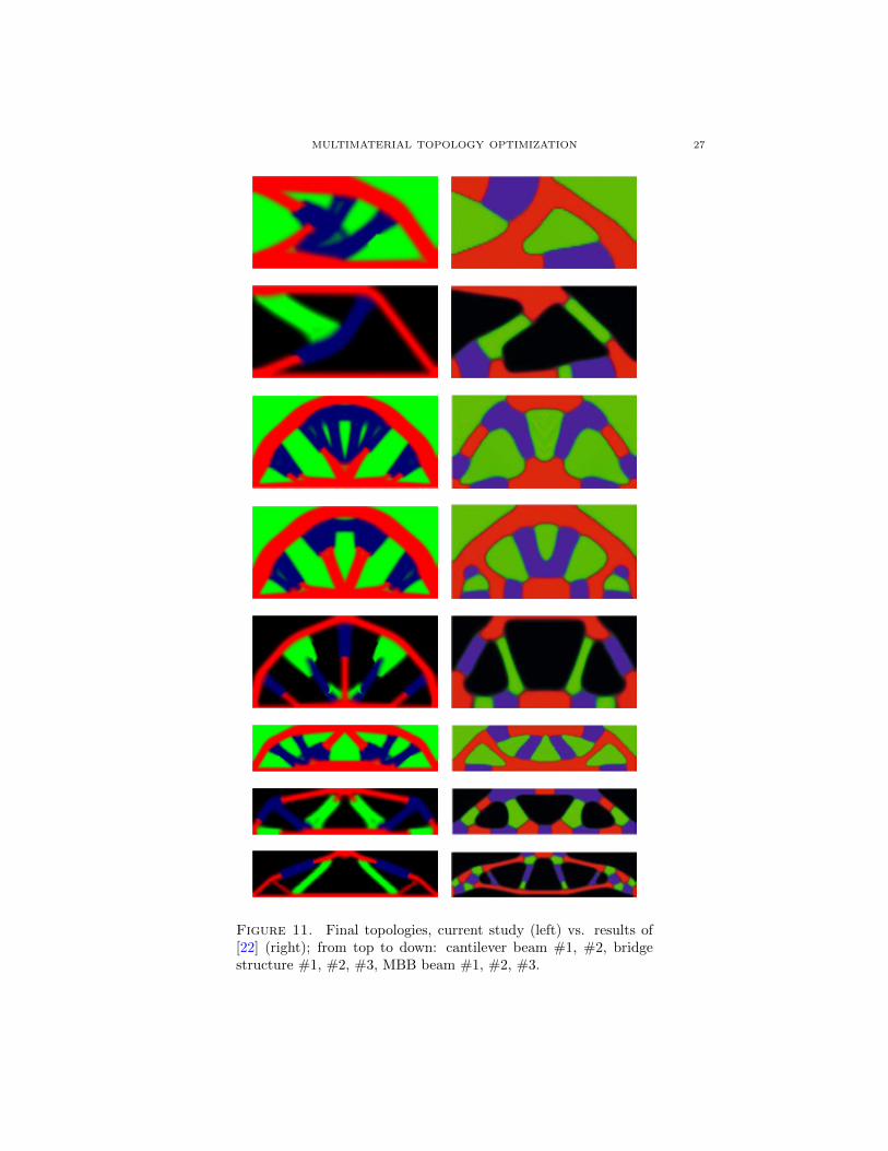
Figure 11. Final topologies, current study (left) vs. results of[22] (right); from top to down: cantilever beam #1, #2, bridgestructure #1, #2, #3, MBB beam #1, #2, #3.


Discussion. The plots in figures 2 to 9 show the success of the presented multi-phase topology optimization framework. Considering figure 10, the convergence ofthe presented code is similar to that of original bi-material topology optimizationcode (note that optimality criteria approach is not a strictly monotone algorithm).This observation illustrates that the presented algorithm inherits the convergenceproperties of its mother algorithm. Considering the reported CPU times and thenumber of outer iterations, it appears that the computational cost of the presentedalgorithm for p phase is about p(p−1)/2 times of the computational cost of the cor-responding binary phase topology optimization algorithm. Therefore, the compu-tational cost is proportional to p2. Because the same sets of controlling parametersare used in this section for all cases, the algorithm’s parameters are not stronglydepend on the type of problem. This observation increases the utility of the pre-sented approach. Comparison of our results with [22] shows that the global outlineof final topologies are similar, however, there are significant differences in details ofresulted topologies. Comparing the structural performance and restructurability ofresulted structures appears to be an interesting issue.

7.2. Minimum thermal compliance topology optimization. The numericalresults corresponding to the model problem mentioned in section 5.2 is presentedin this section. For this purpose, two minimum thermal compliance topology opti-mization problems are considered here; see figure 12. The first problem is adaptedfrom [36] and the second one is adapted from section 5.1.6 of [3]. The design opti-mization parameters corresponding to thermal test problems are listed in table 3.The symmetries of problems are exploited in our simulation to reduce the compu-tational cost. Note that the values of parameters which are not determined hereare taken equal to those of section 7.1 (to show the ability of framework to managedifferent kind of problems using the same set of controlling parameters).

The history of objective function during the optimization iterations (outer iter-ations) is plotted in figure 13 for test cases1 #1, #2 and #3. Except for the case 2#2 (in which the optimization is terminated at iter out = 673 ), the optimizationis stopped after iter max out other iterations in all cases. The variation of filterradius (rf) during optimization cycles is plotted in figure 14 for cases 2 #2, #3.The final topology corresponding to the above mentioned test problems, are shownin figure 15. The colors are selected such that the conductivity decreases based onthe following order: red, blue, green, black and white. The consumed CPU timecorresponding to these experiments are listed in table 4.

Discussion. Similar to the previous section, the results of this section confirmthe convergence and success of the presented algorithm. Considering the results ofcase 2 #1, the algorithm did not converge to stopping criteria based on the mini-mal change in the resulted topology during outer cycles. Checking the topologicalchanges at the later iterations in this case shows the oscillatory behavior in theobjective function values (in fact algorithm does not proceed toward a better out-come by additional iterations). This observation suggests to consider a more robustconvergence criteria to improve the computational performance. According to Fig-ure 14, the filter radius decreases monotonically during the optimization iterations.According to our numerical experiment, using a better strategy for updating filterradius could improve the convergence speed and also the termination criteria.


u = 0 u = 0

u = 0

u = 0

?

Thermal Case 1

u = 0 ?

Thermal Case 2

Figure 12. Geometries and boundary conditions correspondingto minimum thermal compliance model problems .

Table 3. Design parameters of minimum thermal compliancetopology optimization test cases.

Problem nx ny p e v iter max out

Case1 #1 50 50 3 [4 2 1]′ [0.35 0.35 0.3]′ 100

Case1 #2 50 50 4 [6 4 2 1]′ [0.25 0.25 0.25 0.25]′ 100

Case1 #3 50 50 5 [8 6 4 2 1]′ [0.2 0.2 0.2 0.2 0.2]′ 100

Case2 #1 100 50 3 [1.e4 1.e3 1]′ [0.25 0.25 0.5]′ 1000

Case2 #2 100 50 4 [1.e4 5.e3 1.e3 1]′ [0.2 0.15 0.15 0.5]′ 1000

Case2 #3 100 50 5 [1.e3 4.e2 2.e2 1.e2 1]′ [0.2 0.1 0.1 0.1 0.5]′ 400

Table 4. Minimum thermal compliance topology optimizationtest cases: CPU times in second.

Case1#1 Case1#2 Case1#3 Case2#1 Case2#2 Case2#3

38 61 87 730 731 781

0 10 20 30 40 50 60 70 80 90 1004

4.5

5

5.5

6

6.5

7

7.5

8

8.5

9x 10

5

Iteration

Ob

jective

Fu

nctio

n

(a) thermal case 1#1

0 10 20 30 40 50 60 70 80 903

4

5

6

7

8

9x 10

5

Iteration

Ob

jective

Fu

nctio

n

(b) thermal case 1#2

0 10 20 30 40 50 60 70 80 90 1002

3

4

5

6

7

8x 10

5

Iteration

Ob

jective

Fu

nctio

n

(c) thermal case 1#3

Figure 13. The history of objective functional for thermal prob-lem 1 in this study.


0 100 200 300 400 500 600 7002

3

4

5

6

7

8

Iteration

Filt

er

Ra

dio

us

(a) thermal case 2#2

0 50 100 150 200 250 300 350 4002

3

4

5

6

7

8

Iteration

Filt

er

Ra

dio

us

(b) thermal case 2#3

Figure 14. The variation of filter radius during minimum ther-mal compliance topology optimization cycles for cases 2#2 and2#3.

(a) thermal case 1#1 (b) thermal case 1#2 (c) thermal case 1#3

(d) thermal case 2#1 (e) thermal case 2#2 (f) thermal case 2#3

Figure 15. The final topology corresponding to the minimumthermal compliance test cases.


(a) 48 24

(b) 96 48

(c) 192 96

Figure 16. Final topology of MBB− Beam #2 test problem ondifferent grid resolution.

7.3. Grid resolution study. To study the dependence of numerical results to themesh size, the solution of MBB− Beam #2 problem is considered here with threedifferent mesh resolutions: 48× 24, 96× 48 and 192× 96. Because the filter pa-rameter rf controls the length scale in our algorithm, it is selected based on the gridresolution; rf = 4, 8, 16 for these three resolutions respectively. Other parametersare similar to MBB− Beam #2 test case in section 7.1. Results of this experimentare shown in figure 16. Note that for the grid resolution 48× 24, the algorithmterminated at iteration 178, because of meeting the convergence criterion.

Discussion. According to figure 16, the final topology is almost insensitive tothe resolution of computational grid, using a consistent length-scale control.

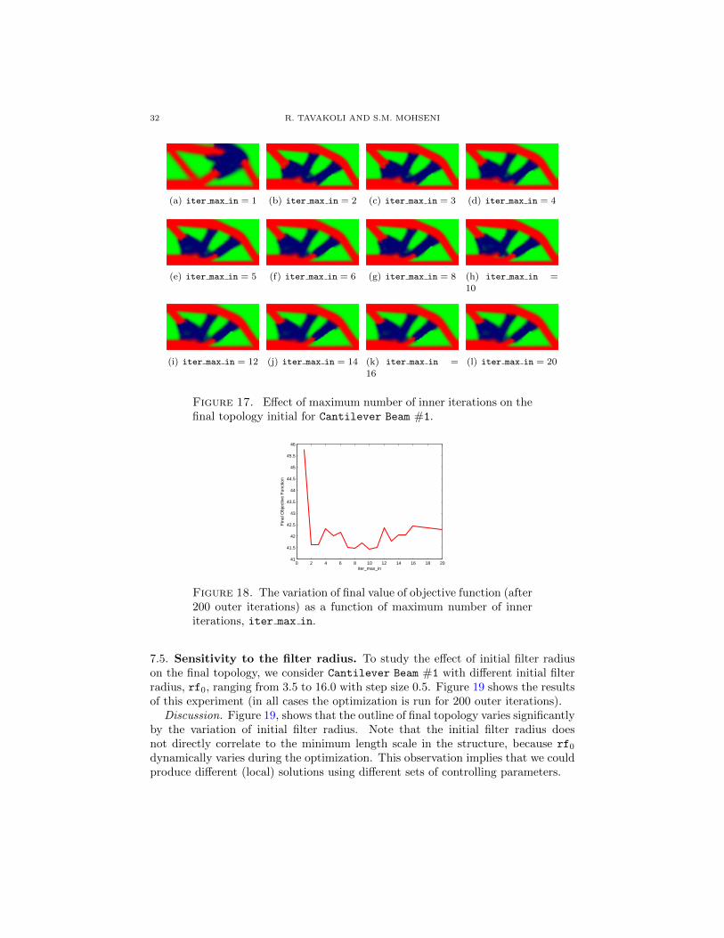
7.4. Sensitivity to the maximum inner iterations (iter max in). The effectof maximum number of inner iterations, iter max in, on the performance and resultof the presented algorithm is numerically studied in this section. For this purpose,the solution of Cantilever Beam #1 with different iter max in is considered here(iter max in = 1, 2, . . . , 20). Figure 17 shows the results of this numerical experi-ment. The variation of final value of objective function (after 200 outer iterations)by iter max in is plotted in figure 18.

Discussion. According to figure 17, the final topology is almost insensitive to thevariation of iter max in for iter max in > 2. Considering figure 18, increasingthe value of iter max in to 20 not only does not improve the convergence of outeriterations but also slightly decreases the overall convergence rate. It is while thecomputational cost increases linearly with iter max in. Therefore, there is anoptimal value for iter max in parameter. According to our numerical experimentsin this study iter max in = 2 is almost an optimal choice.


(a) iter max in = 1 (b) iter max in = 2 (c) iter max in = 3 (d) iter max in = 4

(e) iter max in = 5 (f) iter max in = 6 (g) iter max in = 8 (h) iter max in =

10

(i) iter max in = 12 (j) iter max in = 14 (k) iter max in =

16

(l) iter max in = 20

Figure 17. Effect of maximum number of inner iterations on thefinal topology initial for Cantilever Beam #1.

0 2 4 6 8 10 12 14 16 18 2041

41.5

42

42.5

43

43.5

44

44.5

45

45.5

46

iter_max_in

Fin

al O

bje

ctive

Fu

nctio

n

Figure 18. The variation of final value of objective function (after200 outer iterations) as a function of maximum number of inneriterations, iter max in.

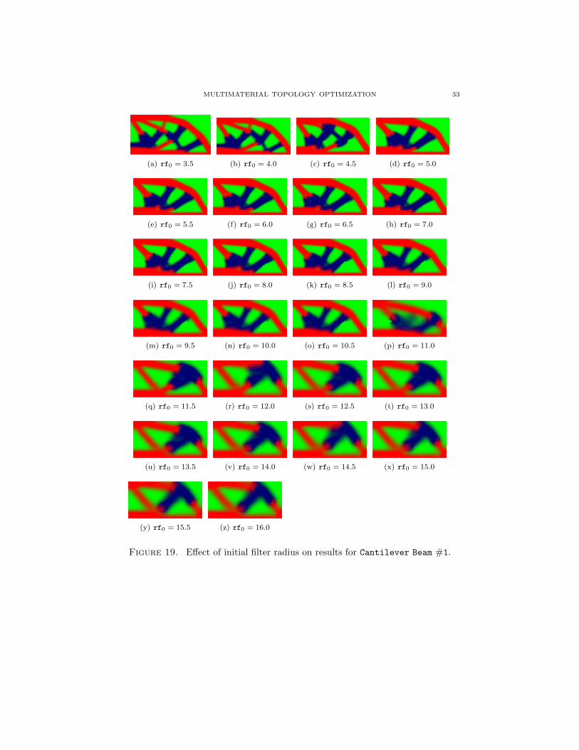
7.5. Sensitivity to the filter radius. To study the effect of initial filter radiuson the final topology, we consider Cantilever Beam #1 with different initial filterradius, rf0, ranging from 3.5 to 16.0 with step size 0.5. Figure 19 shows the resultsof this experiment (in all cases the optimization is run for 200 outer iterations).

Discussion. Figure 19, shows that the outline of final topology varies significantlyby the variation of initial filter radius. Note that the initial filter radius doesnot directly correlate to the minimum length scale in the structure, because rf0

dynamically varies during the optimization. This observation implies that we couldproduce different (local) solutions using different sets of controlling parameters.


(a) rf0 = 3.5 (b) rf0 = 4.0 (c) rf0 = 4.5 (d) rf0 = 5.0

(e) rf0 = 5.5 (f) rf0 = 6.0 (g) rf0 = 6.5 (h) rf0 = 7.0

(i) rf0 = 7.5 (j) rf0 = 8.0 (k) rf0 = 8.5 (l) rf0 = 9.0

(m) rf0 = 9.5 (n) rf0 = 10.0 (o) rf0 = 10.5 (p) rf0 = 11.0

(q) rf0 = 11.5 (r) rf0 = 12.0 (s) rf0 = 12.5 (t) rf0 = 13.0

(u) rf0 = 13.5 (v) rf0 = 14.0 (w) rf0 = 14.5 (x) rf0 = 15.0

(y) rf0 = 15.5 (z) rf0 = 16.0

Figure 19. Effect of initial filter radius on results for Cantilever Beam #1.


8. Summary

Combining the classical binary phase topology optimization algorithm and the(Gauss-Seidel-like) block coordinate descent algorithm, a general framework is in-troduced to solve multimaterials topology optimization problems. The algorithmis easy to implement and almost every binary phase topology optimization solvercould be easily extended to its multiphase counterpart using the presented frame-work; such that the resulted solver inherits the convergence properties of its originalsolver. The overall algorithmic complexity and coding of the presented approach isindependent of the number of contributing phases. Using the presented framework,the classical optimality criteria based binary phase minimum compliance topologyoptimization MATLAB code is extended to solve multiphase thermal and struc-tural topology optimization problems. The success and efficiency of the presentedalgorithm is illustrated numerically by solution of several test problems.

References

[1] M.P. Bendsøe and N. Kikuchi. Generating optimal topologies in structural designusing a homogenization method. Comput Meth Appl Mech Engng, 71(2):197–224,1988.

[2] M.P. Bendsøe. Optimization of structural topology, shape, and material. SpringerVerlag, 1995.

[3] M.P. Bendsøe and O. Sigmund. Topology Optimization: theory, methods and appli-cations. Springer, 2004.

[4] M.P. Bendsøe and O. Sigmund. Material interpolation schemes in topology optimiza-tion. Arch Appl Mech, 69(9):635–654, 1999.

[5] G. Allaire. Shape optimization by the homogenization method. New York, Springer-Verlag, 2002., 2002.

[6] O. Sigmund and S. Torquato. Composites with extremal thermal expansion coeffi-cients. Appl Phys Lett, 69(21):3203–3205, 1996.

[7] O. Sigmund and S. Torquato. Design of materials with extreme thermal expansionusing a three-phase topology optimization method. J Mech Phys Solids, 45(6):1037–1067, 1997.

[8] O. Sigmund and S. Torquato. Design of smart composite materials using topologyoptimization. Smart Materials and Structures, 8:365, 1999.

[9] L.V. Gibiansky and O. Sigmund. Multiphase composites with extremal bulk modulus.J Mech Phys Solids, 48(3):461–498, 2000.

[10] O. Sigmund. Recent developments in extremal material design. in Trends in Compu-tational Mechanics, W.A. Wall, K.-U. Bletzinger and K. Schweizerhof (eds), pages228–232, 2001.

[11] R. Tavakoli and H. Zhang. A nonmonotone spectral projected gradient method forlarge-scale topology optimization problems. Numerical Algebra, Control and Opti-mization, 2(2):395–412, 2012.

[12] B. Bourdin and A. Chambolle. Design-dependent loads in topology optimization.ESAIM COCV, 9:19–48, 2003.

[13] M.Y. Wang and S. Zhou. Synthesis of shape and topology of multi-material structureswith a phase-field method. J Comput-Aided Mater Des, 11(2):117–138, 2004.

[14] H.K. Zhao, T. Chan, B. Merriman, and S. Osher. A variational level set approach tomultiphase motion. J Comput Phys, 127(1):179–195, 1996.

[15] L.A. Vese and T.F. Chan. A multiphase level set framework for image segmentationusing the mumford and shah model. Int J Comput Vis, 50(3):271–293, 2002.

[16] M. Yulin and W. Xiaoming. A level set method for structural topology optimizationand its applications. Adv Eng Softw, 35(7):415–441, 2004.


[17] M.Y. Wang and X. Wang. color level sets: a multi-phase method for structuraltopology optimization with multiple materials. Comput Meth Appl Mech Engng,193(6):469–496, 2004.

[18] M.Y. Wang and X. Wang. A level-set based variational method for design and opti-mization of heterogeneous objects. Computer-Aided Design, 37(3):321–337, 2005.

[19] P. Wei and M.Y. Wang. Piecewise constant level set method for structural topologyoptimization. Int J Numer Methods Eng, 78(4):379–402, 2009.

[20] Z. Luo, L. Tong, J. Luo, P. Wei, and M.Y. Wang. Design of piezoelectric actua-tors using a multiphase level set method of piecewise constants. J Comput Phys,228(7):2643–2659, 2009.

[21] S. Zhou and M.Y. Wang. 3d multi-material structural topology optimization with thegeneralized cahn-hilliard equations. CMES: Comput Model in Eng Sci, 16(2):83–102,2006.

[22] S. Zhou and M.Y. Wang. Multimaterial structural topology optimization with ageneralized cahn–hilliard model of multiphase transition. Struct Multidisc Optim,33(2):89–111, 2007.

[23] X. Huang, M. Xie, et al. Evolutionary topology optimization of continuum structures:methods and applications. Wiley, 2010.

[24] X. Huang and YM Xie. Bi-directional evolutionary topology optimization of contin-uum structures with one or multiple materials. Comput Mech, 43(3):393–401, 2009.

[25] Z. Hashin and S. Shtrikman. A variational approach to the theory of the elasticbehaviour of multiphase materials. J Mech Phys Solids, 11(2):127–140, 1963.

[26] O. Sigmund and J. Petersson. Numerical instabilities in topology optimization: a sur-vey on procedures dealing with checkerboards, mesh-dependencies and local minima.Struct Multidisc Optim, 16(1):68–75, 1998.

[27] W.I. Zangwill. Nonlinear programming: a unified approach. Prentice-Hall EnglewoodCliffs, NJ, 1969.

[28] D.G. Luenberger and Y. Ye. Linear and nonlinear programming, third edition.Springer Verlag, 2008.

[29] JC Bezdek, RJ Hathaway, RE Howard, CA Wilson, and MP Windham. Local conver-gence analysis of a grouped variable version of coordinate descent. J Optim TheoryAppl, 54(3):471–477, 1987.

[30] P. Tseng. Convergence of a block coordinate descent method for nondifferentiableminimization. J Optim Theory Appl, 109(3):475–494, 2001.

[31] C.J. Lin, S. Lucidi, L. Palagi, A. Risi, and M. Sciandrone. Decomposition algorithmmodel for singly linearly-constrained problems subject to lower and upper bounds. JOptim Theory Appl, 141(1):107–126, 2009.

[32] P. Tseng and S. Yun. A coordinate gradient descent method for linearly constrainedsmooth optimization and support vector machines training. Comput Optim Appl,47(2):179–206, 2010.

[33] G. Liuzzi, L. Palagi, and M. Piacentini. On the convergence of a jacobi-type algo-rithm for singly linearly-constrained problems subject to simple bounds. Optim Lett,5(2):347–362, 2011.

[34] O. Sigmund. A 99 line topology optimization code written in matlab. Struct MultidiscOptim, 21(2):120–127, 2001.

[35] E. Andreassen, A. Clausen, M. Schevenels, B.S. Lazarov, and O. Sigmund. Efficienttopology optimization in matlab using 88 lines of code. Struct Multidisc Optim,43(1):1–16, 2011.

[36] Alberto Donoso and Pablo Pedregal. Optimal design of 2d conducting graded ma-terials by minimizing quadratic functionals in the field. Struct Multidisc Optim,30(5):360–367, 2005.


Supplement A. 115-line MATLAB code for multimaterials minimumcompliance topology optimization

The following code includes the 115 lines MATLAB code for the solution ofmultimaterials minimum compliance topology optimization problem. The loadingand boundary conditions are related to MBB-beam case in which only one half ofdomain is considered (the visualization is performed for whole beam).

1 %% 115 LINES MATLAB CODE MULTIPHASE MINIMUM COMPLIANCE TOPOLOGY OPTIMIZATION

2 function multitop(nx,ny,tol_out,tol_f,iter_max_in,iter_max_out,p,q,e,v,rf)


4 for i = 1:p

5 alpha(:,i) = v(i);

6 end

7 %% MAKE FILTER





12 for a = 1:p

13 for b = a+1:p

14 [obj,alpha] = bi_top(a,b,nx,ny,p,v,e,q,alpha,H,Hs,iter_max_in);

15 end

16 end




20 %% UPDATE FILTER



23 end

24 %% SCREEN OUT TEMPORAL TOPOLOGY EVERY 5 ITERATIONS

25 if mod(iter_out,5)==0


27 image([flipdim(I ,2) I]), axis image off, drawnow;

28 end

29 end

30 end

31 %% MAKE FILTER



34 iH = ones(nx*ny*(2*ir+1)^2,1);

35 jH = ones(size(iH)); sH = zeros(size(iH)); k = 0;

36 for i1 = 1:nx

37 for j1 = 1:ny

38 e1 = (i1-1)*ny+j1;





43 end

44 end

45 end

46 end


48 end

49 %% MODIFIED BINARY-PHASE TOPOLOGY OPTIMIZATION SOLVER


50 function [o,alpha] = bi_top(a,b,nx,ny,p,v,e,q,alpha_old,H,Hs,iter_max_in)

51 alpha = alpha_old; iter_in = 0; nu = 0.3;


53 A11 = [12 3 -6 -3; 3 12 3 0; -6 3 12 -3; -3 0 -3 12];

54 A12 = [-6 -3 0 3; -3 -6 -3 -6; 0 -3 -6 3; 3 -6 3 -6];

55 B11 = [-4 3 -2 9; 3 -4 -9 4; -2 -9 -4 -3; 9 4 -3 -4];

56 B12 = [ 2 -3 4 -9; -3 2 9 -2; 4 9 2 3; -9 -2 3 2];

57 KE = 1/(1-nu^2)/24*([A11 A12;A12’ A11]+nu*[B11 B12;B12’ B11]);


59 edofVec = reshape(2*nodenrs(1:end-1,1:end-1)+1,nx*ny,1);

60 edofMat = repmat(edofVec,1,8)+repmat([0 1 2*ny+[2 3 0 1] -2 -1],nx*ny,1);



63 %% DEFINE LOADS AND SUPPORTS (HALF MBB-BEAM)

64 F = sparse(2,1,-1,2*(ny+1)*(nx+1),1); % MBB

65 fixeddofs = union([1:2:2*(ny+1)],[2*(nx+1)*(ny+1)]);

66 U = zeros(2*(ny+1)*(nx+1),1);

67 alldofs = [1:2*(ny+1)*(nx+1)];





72 %% FE-ANALYSIS

73 E = e(1)*alpha(:,1).^q;

74 for phase = 2:p


76 end











87 move = 0.2;


89 for k = 1:p

90 if (k ~= a) && (k ~= b)

91 r = r - alpha(:,k);

92 end

93 end




97 l1 = 0; l2 = 1e9;

98 while (l2-l1)/(l1+l2) > 1e-3

99 lmid = 0.5*(l2+l1);



102 end



105 end

106 end

107 %% MAKE BITMAP IMAGE OF MULTIPHASE TOPOLOGY



109 color = [1 0 0; 0 0 .45; 0 1 0; 0 0 0; 1 1 1];


111 for j = 1:p

112 I(:,1:3) = I(:,1:3) + alpha(:,j)*color(j,1:3);

113 end


115 end

The following pieces of MATLAB code is related to parameter set and main func-tions to solve MBB− Beam #3 test problem.

function [nx,ny,tol,tolf,im_in,im_out,p,q,e,v,rf] = set_parameters ()

nx = 96; ny = 48; tol = 0.001; tolf = 0.05; im_in = 2; im_out = 200;

p = 4; q = 3; e = [9 3 1 1e-9]’; v = [0.16 0.08 0.08 0.68]’; rf = 8;

end

function main

[nx,ny,tol_out,tol_f,iter_max_in,iter_max_out,p,q,e,v,rf] = set_parameters ();

multitop(nx,ny,tol_out,tol_f,iter_max_in,iter_max_out,p,q,e,v,rf);

end

Supplement B. 115-line MATLAB code for multimaterials minimumthermal compliance topology optimization

The following code includes the 115 lines MATLAB code for the solution ofmultimaterials minimum thermal compliance topology optimization problem. Theloading and boundary conditions are related to case #2 of our thermal test prob-lems.

1 %% 115 LINES MATLAB CODE MULTIPHASE THERMAL TOPOLOGY OPTIMIZATION

2 function multitop_h(nx,ny,tol_out,tol_f,iter_max_in,iter_max_out,p,q,e,v,rf)


4 for i = 1:p

5 alpha(:,i) = v(i);

6 end

7 %% MAKE FILTER





12 for a = 1:p

13 for b = a+1:p

14 [obj,alpha] = bi_top_h(a,b,nx,ny,p,v,e,q,alpha,H,Hs,iter_max_in);

15 end

16 end




20 %% UPDATE FILTER



23 end

24 %% SCREEN OUT TEMPORAL TOPOLOGY EVERY 5 ITERATIONS


25 if (mod(iter_out,5)==0)


27 I = [flipdim(I,1); I]; image(I), axis image off, drawnow;

28 end

29 end

30 end

31 %% MAKE FILTER



34 iH = ones(nx*ny*(2*ir+1)^2,1);

35 jH = ones(size(iH));

36 sH = zeros(size(iH));

37 k = 0;

38 for i1 = 1:nx

39 for j1 = 1:ny

40 e1 = (i1-1)*ny+j1;





45 end

46 end

47 end

48 end


50 end

51 %% MODIFIED BINARY-PHASE TOPOLOGY OPTIMIZATION SOLVER

52 function [o,alpha] = bi_top_h(a,b,nx,ny,p,v,e,q,alpha_old,H,Hs,iter_max_in)

53 alpha = alpha_old; iter_in = 0;


55 KE = [2/3 -1/6 -1/3 -1/6; -1/6 2/3 -1/6 -1/3; ...

56 -1/3 -1/6 2/3 -1/6; -1/6 -1/3 -1/6 2/3];


58 edofVec = reshape(nodenrs(1:end-1,1:end-1)+1,nx*ny,1);

59 edofMat = repmat(edofVec,1,4)+repmat([0 ny+[1 0] -1],nx*ny,1);



62 %% DEFINE LOADS AND SUPPORTS

63 F = sparse((ny+1)*(nx+1),1); F(:,1) = 1;

64 %fixeddofs = union([1:ny+1],[(ny+1):(ny+1):(nx+1)*(ny+1)]); %case1

65 fixeddofs = [1:5]; % case 2

66 U = zeros((ny+1)*(nx+1),1);

67 alldofs = [1:(ny+1)*(nx+1)];





72 %% FE-ANALYSIS

73 E = e(1)*alpha(:,1).^q;

74 for phase = 2:p


76 end












87 move = 0.2;


89 for k = 1:p

90 if (k ~= a) && (k ~= b)

91 r = r - alpha(:,k);

92 end

93 end




97 l1 = 0; l2 = 1e9;

98 while (l2-l1)/(l1+l2) > 1e-3

99 lmid = 0.5*(l2+l1);



102 end



105 end

106 end

107 %% MAKE BITMAP IMAGE OF MULTIPHASE TOPOLOGY


109 color = [1 0 0; 0 0 .45; 0 1 0; 0 0 0; 1 1 1];


111 for j = 1:p

112 I(:,1:3) = I(:,1:3) + alpha(:,j)*color(j,1:3);

113 end


115 end

The following pieces of MATLAB code is related to parameter set and main func-tions to solve Case2 #3 test problem.

function [nx,ny,tol,tolf,im_in,im_out,p,q,e,v,rf] = set_parameters ()

nx = 100; ny = 50; tol = 0.001; tolf = 0.05; im_in = 2; im_out = 400;

p = 5; q = 3; e = [1000 400 200 100 1]’; v = [0.2 0.1 0.1 0.1 0.5]’; rf = 8;

end

function main_h

[nx,ny,tol_out,tol_f,iter_max_in,iter_max_out,p,q,e,v,rf] = set_parameters ();

multitop_h(nx,ny,tol_out,tol_f,iter_max_in,iter_max_out,p,q,e,v,rf);

end

Documents

Multimaterial topology optimization · alternating active-phase algorithm for multimaterial topology optimization problems a 115-line matlab implementation r. tavakoli and s.m. mohseni