Multilinear Algebra and Applications (2MMD20,

Fall 2015)

Jan Draisma

CHAPTER 1

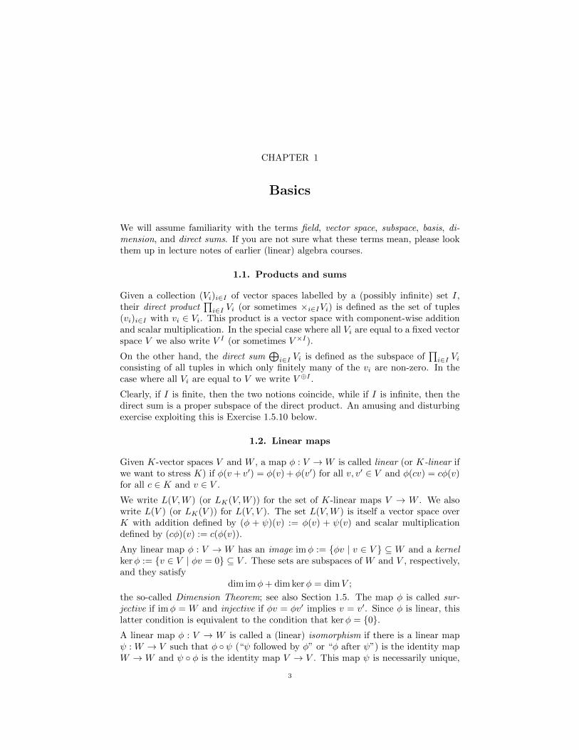
Basics

We will assume familiarity with the terms field, vector space, subspace, basis, di-mension, and direct sums. If you are not sure what these terms mean, please lookthem up in lecture notes of earlier (linear) algebra courses.

1.1. Products and sums

Given a collection (Vi)i∈I of vector spaces labelled by a (possibly infinite) set I,their direct product

∏i∈I Vi (or sometimes ×i∈IVi) is defined as the set of tuples

(vi)i∈I with vi ∈ Vi. This product is a vector space with component-wise additionand scalar multiplication. In the special case where all Vi are equal to a fixed vectorspace V we also write V I (or sometimes V ×I).

On the other hand, the direct sum⊕

i∈I Vi is defined as the subspace of∏i∈I Vi

consisting of all tuples in which only finitely many of the vi are non-zero. In thecase where all Vi are equal to V we write V ⊕I .

Clearly, if I is finite, then the two notions coincide, while if I is infinite, then thedirect sum is a proper subspace of the direct product. An amusing and disturbingexercise exploiting this is Exercise 1.5.10 below.

1.2. Linear maps

Given K-vector spaces V and W , a map φ : V →W is called linear (or K-linear ifwe want to stress K) if φ(v+ v′) = φ(v) + φ(v′) for all v, v′ ∈ V and φ(cv) = cφ(v)for all c ∈ K and v ∈ V .

We write L(V,W ) (or LK(V,W )) for the set of K-linear maps V → W . We alsowrite L(V ) (or LK(V )) for L(V, V ). The set L(V,W ) is itself a vector space overK with addition defined by (φ + ψ)(v) := φ(v) + ψ(v) and scalar multiplicationdefined by (cφ)(v) := c(φ(v)).

Any linear map φ : V → W has an image imφ := {φv | v ∈ V } ⊆ W and a kernelkerφ := {v ∈ V | φv = 0} ⊆ V . These sets are subspaces of W and V , respectively,and they satisfy

dim imφ+ dim kerφ = dimV ;

the so-called Dimension Theorem; see also Section 1.5. The map φ is called sur-jective if imφ = W and injective if φv = φv′ implies v = v′. Since φ is linear, thislatter condition is equivalent to the condition that kerφ = {0}.A linear map φ : V → W is called a (linear) isomorphism if there is a linear mapψ : W → V such that φ ◦ ψ (“ψ followed by φ” or “φ after ψ”) is the identity mapW → W and ψ ◦ φ is the identity map V → V . This map ψ is necessarily unique,

3

4 1. BASICS

and denoted φ−1. A linear map φ is an isomorphism if and only if it is surjectiveand injective. An isomorphism maps any basis of V to a basis of W , showing thatdimV = dimW .

Suppose we are given a basis (vj)j∈J of V , with J some potentially infinite indexset. Then we have a linear map L(V,W )→W J , φ 7→ (φvj)j∈J . This map is itselfan isomorphism—indeed, if φ is mapped to the all-zero vector in W J , then φ is zeroon a basis of V and hence identically zero. Hence the map L(V,W ) → W J justdescribed is injective. On the other hand, given any vector (wj)j∈J ∈ W J there isa linear map φ : V → W with φvj = wj . Indeed, one defines φ as follows: given v,write it as

∑j∈J cjvj with only finitely many of the cj non-zero (this can be done,

and in a unique way, since the vj form a basis). Then set φv :=∑i cjwj . Hence the

map L(V,W )→W J is surjective. We conclude that it is, indeed, an isomorphism.In particular, this means that the dimension of L(V,W ) is that of W J .

1.3. Matrices and vectors

Given a basis (vj)j∈J of a K-vector space V , we have a linear isomorphism β :K⊕J → V sending a J-tuple (cj)j∈J with only finitely many non-zero entries to thelinear combination

∑j cjvj . Thus we may represent an element v of the abstract

vector space V by means of a J-tuple β−1v of numbers in K.

Given a basis (wi)i∈I of a second K-vector space W with corresponding isomor-phism γ : K⊕I → W and given a linear map φ : V → W , we may represent φ bya matrix A with rows labelled by the elements of I and the columns labelled bythe elements of J , and with (i, j)-entry equal to the j-th coordinate of γ−1(φvi).Note that every column has only finitely many non-zero entries. Conversely, bythe results of the previous section, every I × J-matrix whose columns are elementsof K⊕I is the matrix of a unique linear map V → W . The fundamental relationbetween φ and A is that applying φ on an abstract vector v boils down to perform-ing matrix-vector multiplication of A with the vector β−1v representing v. Moreprecisely, the diagram

Vφ // W

K⊕J

β

OO

x 7→Ax// K⊕I

γ

OO

commutes, i.e., the composition of linear maps along both paths from K⊕J to Wgive the same linear map. Here Ax stands for the product of the I × J-matrix Awith the vector x ∈ K⊕J . Notice that since x has only finitely non-zero entries, thisproduct is well-defined, and since the columns of A are elements ofK⊕I , the productis again an element of K⊕I . When I = {1, . . . , n} and J = {1, . . . ,m} for somenatural numbers m,n, this boils down to ordinary matrix-vector multiplication.

Matrices and column or row vectors will be used whenever we implement linear-algebraic algorithms on a computer. For instance, an m-dimensional subspace ofan n-dimensional vector space W can be described as the image of an injectivelinear map φ : Km → W (here m is necessarily at most n). After a choice ofbasis w1, . . . , wn of W , φ can be represented as an n×m-matrix A as above (wherefor vj , j ∈ J = {1, . . . ,m} we take the standard basis of V = Km). Hence the

1.4. THE DUAL 5

columns of this matrix represent a basis of imφ relative to the chosen basis of W .The matrix A will have rank m.

Exercise 1.3.1. In this setting, two n × m-matrices A and B, both of rank m,represent the same linear subspace of W if and only if there exists an invertiblem×m-matrix g such that Ag = B; prove this.

Exercise 1.3.2. Write a function Intersect in Mathematica which takes as inputtwo full-rank matrices A and B with n rows and at most n columns, and whichoutputs an n×k-matrix C of rank k that represents the intersection of the subspacesrepresented by A and by B. Also write a function Add that computes a full-rankmatrix representing the sum of the spaces represented by A and by B.

Alternatively, a codimension-n subspace of an m-dimensional vector space V canbe represented as the kernel of a surjective map φ : V → Kn (now m is necessarilyat least n); here we use the Dimension Theorem. Choosing a basis v1, . . . , vm of Vand the standard basis in Km, we may represent φ by an n×m-matrix.

Exercise 1.3.3. In this setting, two n × m-matrices A and B, both of rank n,represent the same linear subspace of V if and only if there exists an invertiblen× n-matrix h such that hA = B; prove this.

1.4. The dual

Given a K-vector space V , the dual V ∗ of V is LK(V,K), i.e., the set of all K-linearfunctions V → K.

By the discussion of L(V,W ) in Section 1.2, V ∗ is itself a K-vector space. Moreover,V ∗ has the same dimension as KJ , if J is (the index set of) some basis of V , whileV itself has the same dimension as K⊕J . If, in particular, J is finite, i.e., if V isfinite-dimensional, then V and V ∗ have the same dimension. In general, since K⊕J

is a subspace of KJ , we still have the inequality dimV ≤ dimV ∗.

Exercise 1.4.4. Assume that J is infinite but countable. (A typical example isV = K[t] = 〈1, t, t2, . . .〉K , the K-space of polynomials in a single variable t, withJ = N and basis (tj)j∈N.) Prove that V ∗ does not have a countable basis.

The following generalisation is trickier.

Exercise 1.4.5. Assume that J is infinite but not necessarily countable. Provethat V ∗ has no basis of the same cardinality as J .

Whether V is finite-dimensional or not, there is no natural linear map V → V ∗

that does not involve further choices (e.g. of a basis). However, there is alwaysa natural map V → (V ∗)∗ that sends v ∈ V to the linear function V ∗ → K thatsends x ∈ V ∗ to x(v). This natural map is linear, and also injective: if v is mappedto zero, then this means that for all x ∈ V ∗ we have x(v) = 0, and this meansthat v itself is zero (indeed, otherwise v would be part of some basis (vj)j∈J , sayas vj0 , and one could define a linear function x to be 1 on vj0 and arbitrary on theremaining basis elements; then x(v) 6= 0).

The fact that V → (V ∗)∗ is injective implies that its image has dimension dimV . IfV is finite-dimensional, then by the above we have dimV = dimV ∗ = dim(V ∗)∗, so

6 1. BASICS

that the map V → (V ∗)∗ is actually a linear isomorphism. Informally, we expressthis by saying that for finite-dimensional vector spaces V we have V = (V ∗)∗.In such a statement we mean that we have a natural (or canonical) isomorphismin mind from one space to the other, i.e., an isomorphism that does not involvefurther arbitrary choices. (We are being deliberately vague here about the exactmathematical meaning of the terms natural or canonical.)

Exercise 1.4.6. Replacing V by V ∗ in the above construction, we obtain an injec-tive linear map ψ : V ∗ → ((V ∗)∗)∗. Find a canonical left inverse to this map, thatis, a linear map π : ((V ∗)∗)∗ → V ∗ such that π ◦ ψ is the identity map on V ∗.

A linear map φ : V → W gives rise to a natural linear map φ∗ : W ∗ → V ∗,called the dual of φ and mapping y ∈ W ∗ to the linear function on V defined byv 7→ y(φv). More succinctly, we have φ∗y := y ◦ φ. It is convenient to see this in adiagram: if y is a linear function on W , then φ∗y fits into the following diagram:

Vφ //

φ∗y

W

y

��K.

Note that duality reverses the arrow: from a map V → W one obtains a mapW ∗ → V ∗. The kernel of φ∗ is the set of all linear functions on W that vanishidentically on imφ. For the image of φ∗ see Exercise 1.5.9.

If (vj)j∈J is a basis of V and (wi)i∈I is a basis of W , then we have seen in Section 1.3how to associate an I × J-matrix A with the linear map φ, each column of whichhas only finitely many non-zero elements. We claim that the transpose AT , which isa J × I-matrix each of whose rows has a finite number of non-zero elements, can beused to describe the dual map φ∗, as follows. There is a linear map β∗ : V ∗ → KJ

defined as β∗x = (x(vj))j∈J (and dual to the map β from Section 1.3; check thatKI is the dual of K⊕I), and similarly a linear map γ∗ : W ∗ → KI . Then thediagram

V ∗

β∗

��

W ∗φ∗oo

γ∗

��KJ KI

x 7→AT xoo

commutes. Note that the product ATx is well-defined for every x ∈ KI , as eachrow of AT has only finitely many non-zero entries. In the special case where I andJ are finite, we recover the familiar fact that “the matrix of the dual map withrespect to the dual basis is the transpose of the original matrix”. In the infinitecase, however, note that AT is not the matrix associated to φ∗ with respect to basesof W ∗ and V ∗: e.g., the linear forms xi ∈ W ∗, i ∈ I determined by xi(wi′) = δi,i′

do not span W ∗ as soon as W is infinite-dimensional.

1.5. Quotients

Given a K-vector space V and a subspace U , the quotient V/U of V by U is definedas the set of cosets (“affine translates”) v + U with v running over V . Note that

1.5. QUOTIENTS 7

v+U = v′+U if and only if v− v′ ∈ U . The quotient comes with a surjective mapπ : V → V/U, πv := v+U , and often it is less confusing to write πv instead of v+U .The quotient V/U is a K-vector space with operations π(v) + π(v′) := π(v + v′)and cπ(v) := π(cv) (since the left-hand sides in these definitions do not depend onthe choices of v and v′ representing v + V and v′ + V , one needs to check that theright-hand sides do not depend on these choices, either). The map π is linear withrespect to this vector space structure.

If U ′ is any vector space complement of U in V , i.e., if every element v ∈ V can bewritten in a unique way as u+ u′ with u ∈ U and u′ ∈ U ′ (notation: V = U ⊕ U ′,the direct sum), then the restriction π|U ′ of π to U ′ is an isomorphism U ′ → V/U .Hence dim(V/U) satisfies

dimU + dim(V/U) = dimU + dimU ′ = dimV.

Here we have implicitly used that U has a vector space complement U ′; this holdsif one assumes the Axiom of Choice, as we do throughout.

One application of this is, once again, the Dimension Theorem: If φ : V → W isa linear map, then there is natural isomorphism V/ kerφ → imφ sending π(v) toφ(v). By the above with U replaced by kerφ we find

dim kerφ+ dim imφ = dim kerφ+ dim(V/ kerφ) = dimV.

The following exercise gives a construction that we will use a number of times inthis lecture.

Exercise 1.5.7. Let φ : V →W be a linear map, and let U be a subspace of kerφ.Prove that there exists a unique linear map φ : V/U →W satisfying φ ◦ π = φ.

We say that φ factorises into π and φ, or that the diagram

Vφ //

π

��

W

V/Uφ

==

commutes, i.e., that both paths from V to W yield the same linear map. The entirestatement that φ factorises into π and a unique φ is sometimes depicted as

Vφ //

π

��

W

V/U∃!φ.

==

Exercise 1.5.8. Let W be a subspace of V . Find a natural isomorphism between(V/W )∗ and the subspace W 0 of V ∗ consisting of linear functions that restrict to0 on W (the annihilator of W ), and prove that it is, indeed, an isomorphism.

The previous exercise shows that the dual of a quotient is a subspace of the dual,i.e., duality swaps the notions of quotient and subspace.

Exercise 1.5.9. Let φ : V → W be a linear map. Find a natural isomorphismbetween the image imφ∗ of the dual of φ and (V/ kerφ)∗, and prove that it is,indeed, an isomorphism.

8 1. BASICS

Here is an amusing exercise, where the hint for the second part is that it appearsin the section on quotients; which quotient is relevant here?

Exercise 1.5.10. A countable number of prisoners, labelled by the natural numbersN, will have rational numbers tattooed on their foreheads tomorrow. Each can thensee all other prisoners’ tattoos, but not his own. Then, without any communication,they go back to their cells, where they individually guess the numbers on their ownforeheads. Those who guess correctly are set free, the others have to remain inprison. Today the prisoners can agree on a strategy, formalised as a sequence offunctions gi : QN\{i} → Q, i ∈ N (one for each prisoner) describing their guess as afunction of the tatooed numbers that they can see.

(1) Prove that there exists a strategy that guarantees that all but finitelymany prisoners will be set free.

(2) Does there exist a strategy as in the previous part, where moreover all giare Q-linear functions?

(3) We have implicitly assumed that prisoner i indeed “sees” an element ofQN\{i}, which requires that he can distinguish his fellow prisoners fromone another. Does there exist a strategy when this is not the case?

Here is another amusing variant of this problem. The first part is standard (if youget stuck, ask your colleagues or look it up!), the second part is due to MaartenDerickx, a former Master’s student from Leiden University.

Exercise 1.5.11. Tomorrow, the countably many prisoners will all be put in aqueue, with prisoner 0 seeing all prisoners 1, 2, 3, 4, . . . in front of him, prisoner 1seeing all prisoners 2, 3, 4, . . . in front of him, etc. Then each gets a black or whitehat. Each sees the colours of all hats in front of him, but not his own colour orthe colours behind. Then, each has to guess the colour of his hat: first 0 shoutshis guess (black or white) so that all others can hear it, then 1, etc. Each prisonerhears all guesses behind him before it is his turn, but not whether the guesses werecorrect or not. Afterwards, those who guessed correctly are set free, and those whoguessed incorrectly remain in prison. Today, the prisoners can decide on a strategy.

(1) For each finite natural number n find a strategy such that all prisonerswill guess correctly except possibly the prisoners 0, n, 2n, . . ..

(2) Prove the existence of a strategy where all prisoners guess correctly exceptpossibly prisoner 0.

(3) Generalise the previous exercise to other finite numbers of colours (fixedbefore the strategy meeting).

Given a linear map φ : V → W and linear subspaces V ′ ⊆ V and W ′ ⊆ W suchthat φ maps V ′ into W ′, we have a unique induced linear map φ : V/V ′ → W/W ′

making the diagram

Vφ //

πV/V ′

��

W

πW/W ′

��V/V ′

φ

// W/W ′

commutative (this is just Exercise 1.5.7 with W replaced by W/W ′ and φ replacedby πW/W ′ ◦ φ). Suppose we have a basis (vj)j∈J and a subset J ′ ⊆ J such that

1.5. QUOTIENTS 9

(vj)j∈J′ span (and hence form a basis of) V ′, and similarly a basis (wi)i∈I of Wwith I ′ ⊆ I indexing a basis of W ′. Then the πV/V ′vj with j not in J form a basis

of V/V ′, and the πW/W ′wi with i ∈ I form a basis of W/W ′. The matrix of φ withrespect to these latter bases is the sub-matrix of the matrix of φ with respect tothe original bases, obtained by taking only the rows whose index is in I \ I ′ and thecolumns whose index is in J \ J ′. Schematically, the matrix of φ has the followingblock structure: [

AI′,J′ AI′,J\J′0 AI\I′,J\J′

],

where the 0 block reflects that V ′ is mapped into W ′ (and the matrix AI′,J′ is the

matrix of the restriction φ|V ′ : V ′ →W ′), and where AI\I′,J\J′ is the matrix of φ.

CHAPTER 2

Group actions and linear maps

This chapter deals with group actions on L(V,W ) and on L(V ), where V and Ware (finite-dimensional) vector spaces. The group action on L(V ) is by conjugation,and it will be further analysed in later chapters.

2.1. Actions and orbits

Let G be a group and let X be a set. An action of G on X is a map G×X → X,denoted (g, x) 7→ gx, satisfying the axioms 1x = x and g(hx) = (gh)x for all x ∈ Xand g, h ∈ G. Here 1 is the identity element of the group and gh is the productof g and h in the group. The G-orbit of x ∈ X (or just orbit if G is fixed in thecontext) is Gx := {gx | g ∈ G} ⊆ X.

Remark 2.1.12. The term orbit may be related to the special case where G is thegroup of rotations of three-space around the z-axis, and X is the unit sphere (the“earth”) centered at the origin. Then orbits are trajectories of points on the earth’ssurface; they are all circles parallel to the (x, y)-plane, except the north pole andthe south pole, which are fixed points of the action.

The stabiliser of x ∈ X is Gx := {g ∈ G | gx = x}. An action gives rise (and is, infact, equivalent) to a homomorphism G→ Sym(X), where Sym(X) is the group ofall permutations of X, by means of g 7→ (x 7→ gx); this homomorphism is called apermutation representation of G on X. If these notions are new to you, please lookthem up in textbooks or lecture notes for previous algebra courses!

The relation x ∼ y :⇔ x ∈ Gy is an equivalence relation (if x = gy then y = g−1xand if in addition y = hz then x = (gh)z), hence the orbits Gx, x ∈ X partitionthe set X. Often, in mathematics, classifying objects means describing the orbitsof some group action in detail, while normal forms are representatives of the orbits.

2.2. Left and right multiplication

The most important example in this chapter is the case where X = L(V,W ) andG = GL(V ) × GL(W ). Here GL(V ), the General Linear group, is the subset ofL(V ) consisting of invertible linear maps, with multiplication equal to compositionof linear maps. The action is defined as follows:

(g, h)φ = h ◦ φ ◦ g−1(= hφg−1).

To verify that this is an action, note first that (1, 1)φ = φ (where the 1s stand forthe identity maps on V and on W , respectively), and for the second axiom write

[(g, h)(g′, h′)]φ = (gg′, hh′)φ = hh′φ(gg′)−1 = h(h′φ(g′)−1)g−1 = (g, h)((g′, h′)φ).

11

12 2. GROUP ACTIONS AND LINEAR MAPS

Check that things go wrong if we leave out the inverse in the definition.

Two maps φ, ψ ∈ L(V,W ) are in the same orbit if and only if there exist linearmaps g ∈ GL(V ) and h ∈ GL(W ) such that the following diagram commutes:

Vφ //

g

��

W

h

��V

ψ// W ;

indeed, this is equivalent to ψ = hφg−1. From the diagram it is clear that gmust map kerφ isomorphically onto kerψ, and also induce a linear isomorphismV/ kerφ → V/ kerψ. Similarly, h must map imφ isomorphically onto imψ andinduce a linear isomorphism W/ imφ→W/ imψ.

Conversely, assume that dim kerφ = dim kerψ and dim(V/ kerφ) = dim(V/ kerψ)and dim(W/ imφ) = dim(W/ imψ). Then we claim that φ and ψ are in the sameorbit. Indeed, choose vector space complements V1, V2 of kerφ and kerψ, respec-tively, and vector space complements W1,W2 of imφ, imψ, respectively. By thefirst two dimension assumptions, there exist linear isomorphisms g′ : kerφ→ kerψand g′′ : V1 → V2, which together yield a linear isomorphism g : V → V mappingkerφ onto kerψ. Then define h′ : imφ → imψ by h′(φ(v1)) := ψ(g′′v1) for allv1. This is well-defined because φ maps V1 isomorphically onto imφ. By the lastdimension assumption there exists a linear isomorphism h′′ : W1 → W2, whichtogether with h′ gives a linear isomorphism W → W satisfying h ◦ φ = ψ ◦ g, asrequired.

Note that, if V is finite-dimensional, then the assumption that dim kerφ = dim kerψimplies the other two dimension assumptions. If, moreover, W is also finite-dimensional, then the construction just given shows that the rank of φ completelydetermines its orbit: it consists of all linear maps of the same rank. After choosingbases, this is equivalent to the fact that for n×m-matrices A,B there exist invert-ible square matrices g and h with B = hAg−1 if and only if A and B have the samerank.

Reformulating things entirely in the setting of (finite) matrices, we write GLn =GLn(K) for the group of invertible n×n-matrices with entries in K. Then GLm×GLn acts on the space Mn,m = Mn,m(K) of n×m-matrices by means of (g, h)A =hAg−1, and the orbit of the n×m-matrix

In,m,k :=

[I 00 0

],

where the k× k-block in the upper left corner is an identity matrix, is the set of allrank-k matrices in Mn,m.

Exercise 2.2.13. Let A be the matrix−21 3 −57 −84 −117−3 21 39 63 9327 51 199 308 44369 93 423 651 933

∈M4,5(Q).

(1) Determine the rank k of A.

2.4. COUNTING OVER FINITE FIELDS 13

(2) Determine invertible matrices g, h such that hAg−1 = I4,5,2.

2.3. Orbits and stabilisers

A fundamental observation about general group actions is that for fixed x ∈ X themap G 7→ Gx ⊆ X, g 7→ gx factorises as follows:

G //

π

��

Gx

G/Gx

∃!

;; ,

where π : G → G/Gx is the projection g 7→ gGx mapping g to the left coset gGxand where the dashed map sends gGx to gx—this is well-defined, since if h = gg′

with g′ ∈ Gx, then hx = (gg′)x = g(g′x) = gx by the axioms. The dashed map isa bijection: it is surjective by definition of Gx and it is injective because gx = hximplies that x = g−1(hx) = (g−1h)x so that g′ := g−1h lies in Gx and henceh = gg′ ∈ gGx.

In particular, if G is finite, then G/Gx and Gx have the same cardinality. Moreover,|G/Gx| is the number of left cosets of Gx. As these partition G and all have thesame cardinality |Gx|, we have |G/Gx| = |G|/|Gx|. Hence we find that

|G| = |Gx| · |Gx|;this fundamental equality that can be used to compute |G| if you known |Gx| and|Gx|, or |Gx| if you know |G| and |Gx|, etc.

2.4. Counting over finite fields

In this section we assume that K = Fq, a field with q elements.

Exercise 2.4.14. The group GLn(Fq) is finite; prove that its order is (qn−1)(qn−q)(qn − q2) · · · (qn − qn−1).

Exercise 2.4.15. Consider the action ofG = GL2(Fq) on the setX of 1-dimensionallinear subspaces of F2

q defined by gU := {gu | u ∈ U} for g ∈ G and U a 1-

dimensional linear subspace of F2q.

(1) Show that X consists of a single orbit, and compute its cardinality.(2) Show that the kernel of the corresponding permutation representation

equals the centre Z consisting of all (non-zero) scalar matrices.(3) Deduce that GL2(F2) is isomorphic to the symmetric group on 3 letters.(4) Deduce that the quotient of GL2(F4) by its centre Z (of order 3) is iso-

morphic to the alternating group on 5 letters.

Note that the order can also be written as

q(n2)(qn − 1)(qn−1 − 1) · · · (q − 1)

or asq(n2)(q − 1)n[n]q!,

where the q-factorial is defined as

[n]q! := [n]q[n− 1]q · · · [1]q

14 2. GROUP ACTIONS AND LINEAR MAPS

and the q-bracket [a]q is defined as qa−1q−1 = qa−1 + · · ·+ q1 + 1.

Next we compute the order of the stabiliser in GLn × GLm of the matrix In,m,k;this is the group of tuples (g, h) such that hIn,m,k = In,m,kg. Splitting into blocks:

h =

[h11 h12h21 h22

]and g =

[g11 g12g21 g22

]we find that

hIn,m,k =

[h11 0h21 0

]and In,m,kg =

[g11 g120 0

].

Hence it is necessary and sufficient that g12 and h21 both be zero, and that g11 =h11. So take g21 an arbitrary element of Mm−k,k and g11 an arbitrary element ofGLk and g22 an arbitrary element of GLm−k; for this there are

q(m−k)k+(k2)+(m−k2 )(q − 1)k+(m−k)[k]q![m− k]q! = q(m2 )(q − 1)m[k]q![m− k]q!

possibilities. Then h11 = g11 is fixed, but for h12 and h22 there are still

qk(n−k)+(n−k2 )(q − 1)n−k[n− k]q! = q(n2)−(k2)(q − 1)n−k[n− k]q!

possibilities. Hence the number of matrices of rank equal to k equals

q(m2 )+(n2)(q − 1)m+n[m]q![n]q!

q(m2 )+(n2)−(k2)(q − 1)m+n−k[k]q![m− k]q![n− k]q!

= q(k2)(q−1)k

[m]q![n]q!

[m− k]q![n− k]q![k]q!.

Exercise 2.4.16. Compute the number of k-dimensional subspaces of Fnq . (Hint:these form a single orbit under GLn(Fq). Compute the order of the stabiliser inGLn(Fq) of the k-dimensional space spanned by the first k standard basis vectors.)

2.5. Invariants

Given an action of a group G on a set X, a function (or map) f : X → Y is calledinvariant if f is constant on orbits, or, equivalently, if f(gx) = f(x) for all x ∈ Xand all g ∈ G. Here the co-domain Y can be anything: some finite set, a field, avector space, an algebra, etc.

For example, we have seen that the function Mn,m(K)→ N that maps a matrix toits rank is an invariant under the action of GLm×GLn studied above. And in factit is a complete invariant in the sense that it completely classifies the orbits.

2.6. Conjugation

In the coming weeks we will intensively study another group action, namely, theconjugation action of GL(V ) on L(V ) defined by gA := g◦A◦g−1. We actually neveruse the notation gA, because of potential confusion with our preferred short-handgAg−1 for the right-hand side.

Exercise 2.6.17. Let K = Fq with q odd (so that 1 6= −1). Compute the cardina-lities of of the orbits of the matrices[

2 00 2

],

[1 00 −1

], and

[0 10 0

]under the conjugation action of GL2(Fq).

2.7. SYMMETRIC POLYNOMIALS 15

Throughout the discussion of conjugation we will assume that V is a finite-dimensionalvector space of dimension n. To warm up, here are a number of invariants for thisaction:

(1) rank: of course the rank of A equals that of gAg−1;(2) determinant: we have det(gAg−1) = (det g)(detA)(det g)−1 = detA;(3) trace: using tr(AB) = tr(BA) for linear maps (or matrices) A,B, one

finds that trace is invariant under conjugation;(4) spectrum: this is the set of eigenvalues of A in some fixed algebraic closure

K of K, and it is invariant under conjugation;(5) characteristic polynomial: this is the degree-n polynomial det(tI − A) ∈

K[t], which remains the same when we conjugate A by g.

Exercise 2.6.18. Assume that K = C. Using your knowledge of the Jordannormal form, argue that these invariants, even taken together, are not completein the sense that they do not completely characterise orbits. Do so by giving twosquare matrices A,B of the same size with the property that the above invariantsall coincide, but such that B is not conjugate to A.

Exercise 2.6.19. Let P ∈ K[t] be any polynomial in one variable. Prove that thefunction L(V ) → {yes,no} sending φ to the answer to the question “Is P (φ) thezero map?” is an invariant under conjugation. (Here P (φ) is defined by replacingthe variable t in P by φ and interpreting powers of φ as repeated compositions ofφ with itself.)

Exercise 2.6.20. Let SLn (for Special Linear group) denote the subgroup of GLnconsisting of matrices of determinant 1. Let SLn×SLn act on Mn by left-and-rightmultiplication, i.e., (g, h)A equals hAg−1.

(1) Prove that det : Mn → K is an invariant.(2) Prove that det and rank together form a complete set of invariants.(3) Assume that K = R. Prove that for every continuous function f : Mn →

R invariant under the action there exists a continuous function g : R→ Rsuch that the diagram

Mnf //

det

��

R

Rg

>>

commutes.

In the next two lectures, we will derive a complete set of invariants, and correspond-ing normal forms, for linear maps under conjugation. What makes these normalforms different from the Jordan normal form is that they are completely definedover the original field K, rather than over some extension field.

2.7. Symmetric polynomials

No discussion of invariants is complete without a discussion of symmetric polyno-mials. Let n be a natural number and let G = Sym(n) act on the polynomialring K[x1, . . . , xn] in n variables by πf := f(xπ(1), . . . , xπ(n)), so that, for instance

16 2. GROUP ACTIONS AND LINEAR MAPS

(1, 2, 3)(x21x2 − x2x3) = x22x3 − x1x3). A polynomial f is called symmetric if itis invariant under Sym(n), i.e., if πf = f for all π ∈ Sym(n). In particular, theelementary symmetric polynomials

s1 := x1 + x2 + . . .+ xn

s2 := x1x2 + x1x3 + . . .+ xn−1xn...

sk :=∑

i1<...<ik

xi1 · · ·xik

...

sn := x1x2 · · ·xnare symmetric polynomials. They are in fact a complete set of symmetric polyno-mials, in the following sense.

Theorem 2.7.21. If f is a symmetric polynomial in x1, . . . , xn, then there exists apolynomial g in n variables y1, . . . , yn such that f is obtained from g by replacingyi by si.

In fact, the polynomial g is unique, but we will not need that. The relation ofthis theorem with the notion of invariants above is the following: Sym(n) acts bymeans of linear maps on Kn permuting the standard basis. Symmetric polynomialsgive rise to invariant polynomial functions Kn → K, and the theorem states thatall invariant polynomial functions can be expressed in the elementary symmetricpolynomial functions. Here, strictly speaking, we have to assume that K is infinite,since if it is finite of order q then xq1, while clearly a different polynomial from x1,defines the same polynomial function Kn → K as x1 does.

Proof. Define a linear order on monomials in the xi as follows: xa11 · · ·xann is

larger than xb11 · · ·xbnn if the first non-zero entry of (a1− b1, . . . , an− bn) is positive.Hence the largest monomial of sk equals x1 · · ·xk. It is easy to see that this linearorder is a well-order: there do not exist infinite, strictly decreasing sequences m1 >m2 > . . . of monomials.

The Sym(n)-orbit of a monomial xa11 · · ·xann consists of all monomials of the form

xaπ(1)

1 · · ·xaπ(n)n . Among these, the monomial corresponding to permutations such

that the sequence aπ(1), . . . , aπ(n) decreases (weakly) is the largest monomial.

Now let m = xa11 · · ·xann be the largest monomial with a non-zero coefficient in f .Since f is symmetric, all monomials in the Sym(n)-orbit of m also have non-zerocoefficients in f . Since m is the largest among these, we have a1 ≥ . . . ≥ an.

Now consider the monomial g1 := yann yan−1−ann−1 · · · ya1−a21 . It is easy to see that

the polynomial g1(s1, . . . , sn) obtained by replacing yk by sk has the same largestmonomial m as f . Hence subtracting a suitable scalar multiple we arrive at apolynomial

f1 := f − cg1(s1, . . . , sn)

where the coeffient of m has become zero, so that the largest monomial is strictlysmaller than m. By induction, this proves the theorem. �

2.7. SYMMETRIC POLYNOMIALS 17

The following exercise shows the link with invariants of matrices under conjugation.

Exercise 2.7.22. Take K = C. Let ck : Mn(C) → C be the i-th coefficient of thecharacteristic polynomial, i.e., we have

det(tI −A) = tn + c1(A)tn−1 + . . .+ cn−1(A)t+ cn(A),

so that, in particular, cn(A) = (−1)n detA and c1(A) = − tr(A). Then the ck arepolynomial functions Mn(C)→ C that are invariant under conjugation.

(1) Check that ck(A) = (−1)ksk(λ1, . . . , λn), where λ1, . . . , λn are the eigen-values (listed with multiplicities) of A.

In the following parts, let f : Mn(C)→ C be any polynomial function of the matrixentries that is invariant under conjugation.

(2) Prove that the restriction of f to the space of diagonal matrices, identifiedwith Cn, is a polynomial function of the elementary symmetric polynomi-als in those diagonal entries.

(3) Prove that f itself (on all of Mn(C)) is a polynomial in the functionsc1, . . . , cn. (Hint: you may use that polynomials are continuous functions,and that diagonalisable matrices are dense in Mn(C).

CHAPTER 3

The minimal polynomial and nilpotent maps

In this chapter, we study two important invariants of linear maps under conjugationby invertible linear maps. These are the minimal polynomial on the one hand, whichis defined for any linear map, and a combinatorial object called associated partition,which is defined only for so-called nilpotent linear maps.

3.1. Minimal polynomial

Throughout this chapter, V is a finite-dimensional vector space of dimension nover K, and φ is a linear map from V to itself. We write φ0 for the identitymap I : V → V , φ2 for φ ◦ φ, φ3 for φ ◦ φ ◦ φ, etc. Let p = p(t) ∈ K[t] be apolynomial in one variable t, namely p = c0 + c1t + . . . + cdt

d. Then we definep(φ) := c0I + c1φ+ . . .+ cdφ

d. We say that φ is a root of p if p(φ) is the zero mapV → V . A straightforward calculation shows that the map K[t] → L(V ), p 7→p(φ) is an algebra homomorphism, i.e., it satisfies (p + q)(φ) = p(φ) + q(φ) and(pq)(φ) = p(φ)q(φ) = q(φ)p(φ), where the multiplication in K[t] is multiplicationof polynomials and the multiplication in L(V ) is composition of linear maps. SinceL(V ) has finite dimension over K, the linear maps I, φ, φ2, . . . cannot be all linearlyindependent. Hence the linear map p 7→ p(φ) must have a non-zero kernel I. Thiskernel is an ideal in K[t]: if q, r ∈ I , which means that q(φ) = r(φ) = 0, then alsoq + r ∈ I and pq ∈ I for all p ∈ K[t].

Let pmin be a non-zero polynomial of minimal degree in I that has leading coefficientequal to 1, i.e., which is monic. Every polynomial p ∈ I is a multiple of pmin. Indeed,by division with remainder we can write p = qpmin + r with deg r < deg pmin. Butthen r = p− qpmin lies in I, and hence must be zero since pmin had the least degreeamong non-zero elements of I. Hence p = qpmin. In particular, it follows thatpmin ∈ I with the required properties (minimal degree and monic) is unique, andthis is called the minimal polynomial of φ. The minimal polynomial of a squarematrix is defined in exactly the same manner.

Exercise 3.1.23. Write a Mathematica function MinPol that takes as input asquare integer matrix A and a number p that is either 0 or a prime, and thatoutputs the minimal polynomial of A over Q if p = 0 and the minimal polynomialof A over K = Z/pZ if p is a prime.

Exercise 3.1.24. Show that pmin is an invariant of φ under the conjugation actionof GL(V ) on L(V ).

19

20 3. THE MINIMAL POLYNOMIAL AND NILPOTENT MAPS

3.2. Chopping up space using pmin

The minimal polynomial will guide us in finding the so-called rational Jordan nor-mal form of φ. The first step is the following lemma.

Lemma 3.2.25. Suppose that φ is a root of p · q, where p and q are coprime poly-nomials. Then V splits as a direct sum ker p(φ)⊕ ker q(φ).

Perhaps a warning is in order here: (pq)(φ) = 0 does not imply that one of p(φ), q(φ)must be zero.

Proof. Write 1 = ap + bq for suitable a, b ∈ K[t]; these can be found usingthe extended Euclidean algorithm for polynomials. Then for v ∈ V we have v =a(φ)p(φ)v + b(φ)q(φ)v. The first term lies in ker q(φ), because

q(φ)a(φ)p(φ)v = a(φ)(p(φ)q(φ))v = 0

(while linear maps in general do not commute, polynomials evaluated in φ do—check this if you haven’t already done so). Similarly, the second term b(φ)q(φ)vlies in ker p(φ). This shows that ker p(φ) + ker q(φ) = V . Finally, if v is in theintersection ker p(φ) ∩ ker q(φ), then the above shows that v = 0 + 0 = 0. Hencethe sum in ker p(φ) + ker q(φ) is direct, as claimed. �

Exercise 3.2.26. Prove that, in the setting of the lemma, im p(φ) = ker q(φ) (andvice versa).

In the lemma, both subspaces V1 := ker p(φ) and V2 := ker q(φ) are stable underφ, which means that φ maps Vi into Vi for i = 1, 2. Indeed, if v ∈ V1, thenp(φ)φv = φp(φ)v = 0 so that φv ∈ V1, as well.

Now factor pmin as pm11 · · · pmrr where the pi are distinct, monic, irreducible poly-

nomials in K[t], and the exponents mi are strictly positive. Write qi := pmii . Thepolynomial q1 is coprime with q2 · · · qr. Hence we may apply the lemma and find

V = ker q1(φ)⊕ ker(q2 · · · qr)(φ).

Now let W be the second space on the right-hand side. This space is stable underφ, and the restriction φ|W on it is a root of the polynomial q2 · · · qr. Moreover, q2is coprime with q3 · · · qr. Hence we may apply the lemma with V replaced by W ,φ replaced by φ|W , p replaced by q2 and q replaced by q3 · · · qr to find

W = ker q2(φ|W )⊕ ker(q3 · · · qr)(φ|W ).

Now ker q2(φ) ⊆ V and ker(q3 · · · qr)(φ) ⊆ V are both contained in W , so that wemay as well write

W = ker q2(φ)⊕ ker(q3 · · · qr)(φ),

and hence

V = ker q1(φ)⊕ ker q2(φ)⊕ ker(q3 · · · qr)(φ).

Continuing in this fashion we find that

V =⊕

ker qi(φ);

in what follows we write Vi := ker qi(φ) and φi : Vi → Vi for the restriction of φ toVi.

3.3. THE PARTITION ASSOCIATED TO A NILPOTENT MAP 21

Now recall that we are trying to find invariants and normal forms for linear mapsunder conjugation. Suppose that we have a second element ψ ∈ L(V ) and wantto find out whether it is in the same orbit as φ. First, we have already seen inExercise 3.1.24 that both minimal polynomials must be the same. Moreover, if φ =gψg−1, then for each i = 1, . . . , r, the linear map g maps ker qi(ψ) isomorphicallyonto Vi. This proves that the dimensions of these spaces are invariants. Conversely,if these dimensions are the same for φ and for ψ, then one can choose arbitrarylinear isomorphisms hi : ker qi(ψ) → Vi. These together give a linear isomorphismh : V → V with the property that for ψ′ := hψh−1 we have ker qi(ψ

′) = Vi. Writeψ′i for the restriction of ψ′ to Vi. Of course, ψ and φ are GL(V )-conjugate if andonly if ψ′ and φ are, and this is true if and only if each ψ′i is GL(Vi)-conjugate toeach φi. Indeed, if φi = giψ

′ig−1i , then the gi together define an element g of GL(V )

conjugating ψ′ into φ. Conversely, a g that conjugates ψ′ into φ necessarily leaveseach Vi stable, and the restrictions gi to the Vi conjugate ψ′i into φi.

Now replace φ by a single φi, and V by Vi. The point of all this is that we have thusreduced the search for invariants and normal forms to the case where φ ∈ L(V ) isa root of a polynomial pm with p irreducible and monic. Then it follows that theminimal polynomial of φ itself must also be a power of p; assume that we have takenm minimal, so that pmin = pm. In the next chapter, we will split such a linear mapφ into two commuting parts: a semi-simple part φs whose mimimal polynomial isp itself, and a nilpotent part φn. The remainder of the present chapter deals withthe latter types of matrices.

3.3. The partition associated to a nilpotent map

Starting afresh, let V be a finite-dimensional vector space of dimension n, and letφ ∈ L(V ) be a linear map such that φm = 0 for some sufficiently large nonnegativeinteger m; such linear maps are called nilpotent. Note that any linear map conjugateto φ is then also nilpotent. Let m be the smallest natural number with φm = 0, sothat pmin = tm; m is also called the nilpotency index of φ.

Exercise 3.3.27. In the setting preceding this exercise, fix a non-zero vector v ∈ Vand let p ≥ 0 be the largest exponent for which φpv is non-zero. Prove thatv, φv, . . . , φpv are linearly independent. Derive from this that m, the degree ofpmin, is at most n. If p = n − 1, give the matrix of φ with respect to the basisv, φv, . . . , φn−1v.

Write Vi for imφi; so for i ≥ m we have Vi = {0}. Then we have a chain ofinclusions

V = V0 ⊇ V1 ⊇ · · · ⊇ Vm = {0}.Now note that φ(Vi) = Vi+1, so that φ induces a surjective linear map Vi−1/Vi →Vi/Vi+1. For i ≥ 1 write λi := dimVi−1 − Vi. By surjectivity and by the fact thatφm−1 6= 0 we have λ1 ≥ · · · ≥ λm > 0 = λm+1 = . . .. Moreover, by construction,we have

∑mi=1 λi = n = dimV . A non-increasing sequence (λ1, . . . , λm) of positive

numbers adding up to n is called a partition of n with parts λ1, . . . , λm. We call λthe partition associated to φ—though this is not completely standard terminology:often, the partition associated to φ is defined as the transpose of λ in the followingsense.

22 3. THE MINIMAL POLYNOMIAL AND NILPOTENT MAPS

λ = (5, 5, 2, 1) λ′ = (4, 3, 2, 2, 2)

Figure 1. A Young diagram of a partition and its transpose.

Definition 3.3.28. Given any partition λ = (λ1, . . . , λm) of n, we define a secondpartition λ′ = (λ′1, . . . , λ

′p) of n by p := λ1 and λ′k := |{i ∈ {1, . . . ,m} | λi ≥ k}|.

The partition λ′ is called the transpose of λ.

Why this is called the transpose is best illustrated in terms of Young diagramsdepicting λ and λ′; see Figure 1.

Exercise 3.3.29. Prove that λ′ is, indeed, a partition of n, and that (λ′)′ = λ.

A straightforward check shows that the associated partition is an invariant un-der conjugation. The following theorem states that it is a complete invariant fornilpotent linear maps.

Theorem 3.3.30. Two nilpotent linear maps φ, ψ ∈ L(V ) are in the same orbit ofthe conjugation action of GL(V ) if and only if the partitions of n as constructedabove from φ and ψ are the same. Morever, every partition of n occurs in thismanner.

The proof of the first part of this theorem will be carried out in the next subsection.For the second part, it suffices to exhibit an n×n-matrix giving rise to any partitionλ = (λ1, . . . , λm) of n.

Let λ′ = (λ′1, . . . , λ′p) be the transpose of λ. Let A be the block-diagonal n×n-block

matrix J1 . . .

Jp

where Ji =

0 1

0 1. . .

. . .

0 10

,with λ′i rows and columns (the block consists of a single zero if λ′i equals 1). Weclaim that A gives rise the partition λ in the manner above. Indeed, Ji contributes1 to dim imAk−1 − dim imAk if λ′i ≥ k, and zero otherwise. Hence dim imAk−1 −dim imAk is the number of indices i for which λ′i is at least k. This gives thetranspose of λ′, which is λ itself again.

3.4. Completeness of the associated partition

Given a nilpotent linear map φ ∈ L(V ) with associated partition λ = (λ1, . . . , λm)whose transpose is λ′ = (λ′1, . . . , λ

′p), we will prove that there exists a basis of

V with respect to which φ has the matrix A constructed above. This implies thatany other nilpotent ψ ∈ L(V ) with the same associated partition λ is conjugate to φ.

3.4. COMPLETENESS OF THE ASSOCIATED PARTITION 23

We proceed as follows:

(1) First, choose a basis z1, . . . , zλm of Vm−1.(2) Next, choose y1, . . . , yλm ∈ Vm−2 such that φyi = zi. This is possible

because φ : Vm−2 → Vm−1 is surjective. Now y1 + Vm−1, . . . , yλm +Vm−1 are linearly independent elements of Vm−2/Vm−1, because their φ-images in Vm−1/Vm = Vm−1 are linearly independent. Choose a basisyλm+1 + Vm−1, . . . , yλm−1

+ Vm−1 ∈ Vm−2/Vm−1 of the kernel of the map

φ : Vm−2/Vm−1 → Vm−1/Vm = Vm−1. This means that each φ(yi) = 0.The elements y1, . . . , yλm−1

thus found represent a basis of Vm−2/Vm−1.(3) The pattern is almost clear by now, but there is a catch in the next

step: choose x1, . . . , xλm−1 ∈ Vm−3 such that φxi = yi, and further abasis xλm−1+1 + Vm−2, . . . , xλm−2 + Vm−2 ∈ Vm−3/Vm−2 of the kernel

of induced map φ : Vm−3/Vm−2 → Vm−2/Vm−1. This means that eachφ(xi) is in Vm−1, i.e., is a linear combination of z1, . . . , zλm . Hence, bysubtracting the corresponding linear combinations of y1, . . . , yλm from xiwe obtain a vector xi ∈ Vm−3 that is in the kernel of φ. The vectorsx1 + Vm−2, . . . , xλm−2 + Vm−2 are a basis of Vm−3/Vm−2.

(4) . . . (in the next step, one chooses wλm−2+1, . . . , wλm−3 that map to a basis

of the kernel of φ : Vm−4/Vm−3 → Vm−3/Vm−2. This means that eachφ(wi) is a linear combination of y1, . . . , yλm−1

, z1, . . . , zλm . Subtractingthe corresponding linear combination of x1, . . . , xλm−1

, y1, . . . , yλm , onefinds vectors wi properly in the kernel of φ, etc.) . . . until:

(5) Choose a1, . . . , aλ2 ∈ V0 such that φai = bi, and extend to a basis a1 +V1, . . . , aλ1 + V1 of V0/V1 such that φ(ai) = 0 for i > λ2.

By construction, a1, . . . , aλ1, b1, . . . , bλ2

, . . . , z1, . . . , zλm form a basis of V . Indeed,let v ∈ V . Then there is a unique linear combination a of a1, . . . , aλ1

such thatv−a ∈ V1, and a unique linear combination b of b1, . . . , bλ2

such that v−a−b ∈ V2,etc. We conclude that v is a unique linear combination of the vectors above.

Moreover, each ak generates a Jordan block as follows: φ maps ak 7→ bk 7→ . . . 7→ 0,where the zero appears when the corresponding λi is smaller than k, so that thereare no basis vectors indexed k in that step. In other words, the number of Jordanblocks is equal to λ1, and the k-th Jordan block has size equal to the number of ifor which λi is ≥ k. This is precisely the k-th part λ′k of the transposed partition.

Exercise 3.4.31. Write a Mathematica program that takes as input a nilpotentmatrix and computes the associated partition. Apply this program to the matrix

1 1 −1 0 −10 0 0 0 00 1 0 1 −11 0 −1 −1 01 0 −1 −1 0

.Exercise 3.4.32. Let n = 3 and let K = Fq be a field with q elements.

(1) How many orbits does GL3(K) have by conjugation on the set of nilpotent3× 3-matrices? For each orbit, give a representative matrix A as above.

24 3. THE MINIMAL POLYNOMIAL AND NILPOTENT MAPS

(2) For each of these matrices A, compute the cardinality of the stabiliser{g ∈ GL3(K) | gAg−1 = A} of A, and deduce the cardinality of theseorbits.

As observed out by Jorn van der Pol in Fall 2011, the cardinalities of the orbitsadd up to q6, which gives a check that you carried out the right computation in thesecond part of the exercise. This is, in fact, a general result.

Theorem 3.4.33. The number of nilpotent n× n-matrices over Fq equals qn(n−1).

Various proofs of this fact are known in the literature, but here is one found by An-dries Brouwer and Aart Blokhuis after Jorn’s observation, (also implicit in existingliterature).

Proof. Denote the number of nilpotent n×n-matrices over Fq by an. We firstderive a linear relation among a0, . . . , an, and then by a combinatorial argumentshow that the numbers qk(k−1) satisfy this relation. Since a0 = 1 (the empty matrixis nilpotent) this proves the theorem.

To derive the relation among a0, . . . , an, let φ be a general n × n-matrix, defininga linear map Kn → Kn. Let d be the exponent of t in the minimal polynomialpmin of φ, and write pmin = tdq. By Lemma 3.2.25 we can write V = V0 ⊕ V1 withV0 = kerφd and V1 = ker q(φ). The fact that q is not divisible by t means that itis of the form c+ tq1 with c a non-zero constant and q1 a polynomial. This meansthat the restriction of φ to V1 is invertible (with inverse − 1

c q1(φ)), while of coursethe restriction of φ to V0 is nilpotent. Thus to every linear map φ : Kn → Kn weassociate the four-tuple (V0, V1, φ|V0 , φ|V1) with the third entry a nilpotent linearmap and the fourth entry an invertible linear map. Conversely, splitting Kn intoa direct sum U0 ⊕ U1 and choosing any nilpotent linear map ψ0 : U0 → U0 andany invertible linear map ψ1 : U1 → U1 we obtain a “block-diagonal” linear mapψ : Kn → Kn which restricts to ψ0 on U0 and to ψ1 on U1. Thus we have found twoways to count linear maps Kn → Kn: first, the straightforward way by counting

matrix entries, which gives qn2

, and second, the detour through splitting Kn intoa direct sum U0 ⊕ U1 where U0 has dimension k, say, for which we denote thenumber of possibilities by bk, then choosing a nilpotent linear map in L(U0) (akpossibilities) and an invertible linear map in L(U1) (ck possibilities). This gives theequality

qn2

=

n∑k=0

akbkck.

In this expression we know ck and bk explicitly, namely,

ck = |GLn−k|

bk =|GLn|

|GLk||GLn−k|,

where the expression for bk is explained by choosing a basis of Kn and then lettingU0 be the span of the first k columns and U1 be the span of the last k columns,and accordingly dividing by the number of bases of U0 and U1, respectively. Thuswe obtain

bkck =|GLn||GLk|

= (qn − 1) · · · (qk+1 − 1)q(n2)−(k2).

3.4. COMPLETENESS OF THE ASSOCIATED PARTITION 25

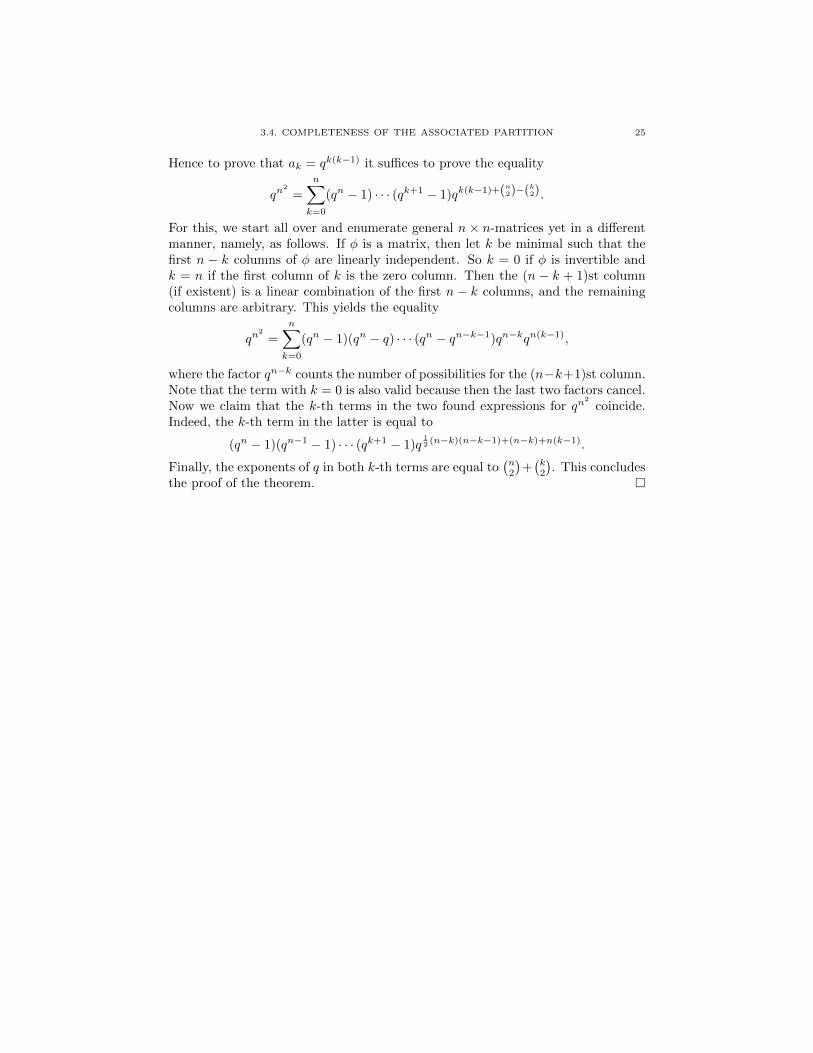
Hence to prove that ak = qk(k−1) it suffices to prove the equality

qn2

=

n∑k=0

(qn − 1) · · · (qk+1 − 1)qk(k−1)+(n2)−(k2).

For this, we start all over and enumerate general n × n-matrices yet in a differentmanner, namely, as follows. If φ is a matrix, then let k be minimal such that thefirst n − k columns of φ are linearly independent. So k = 0 if φ is invertible andk = n if the first column of k is the zero column. Then the (n − k + 1)st column(if existent) is a linear combination of the first n − k columns, and the remainingcolumns are arbitrary. This yields the equality

qn2

=

n∑k=0

(qn − 1)(qn − q) · · · (qn − qn−k−1)qn−kqn(k−1),

where the factor qn−k counts the number of possibilities for the (n−k+1)st column.Note that the term with k = 0 is also valid because then the last two factors cancel.Now we claim that the k-th terms in the two found expressions for qn

2

coincide.Indeed, the k-th term in the latter is equal to

(qn − 1)(qn−1 − 1) · · · (qk+1 − 1)q12 (n−k)(n−k−1)+(n−k)+n(k−1).

Finally, the exponents of q in both k-th terms are equal to(n2

)+(k2

). This concludes

the proof of the theorem. �

CHAPTER 4

Rational Jordan normal form

This chapter concludes our dicussion started in Chapter 3 of linear maps underthe action of conjugation with invertible linear maps. We derive a complete set ofinvariants under a technical assumption on the field, namely, that it is perfect—thisis needed from Section 4.3 on.

4.1. Semisimple linear maps

In Chapter 3 we have seen nilpotent linear maps and their orbits. In this section wewill get acquainted with the other extreme: semisimple linear maps. In the sectionsfollowing this one, we combine results on both types of maps to derive the rationalJordan normal form.

A polynomial p ∈ K[t] is called square-free if it has no factor of the form q2 withq a non-constant polynomial. Writing p as pm1

1 · · · pmrr where the pi are distinctirreducible polynomials and the mi are positive integers, p is square-free if and onlyif all mi are equal to 1. The polynomial f := p1 · · · pr is then called the square-freepart of f . Note that f divides p, while p in turn divides fm where m := maximi.

Now let V be a finite-dimensional vector space. A linear map φ ∈ L(V ) is calledsemisimple if there exists a square-free polynomial p such that p(φ) = 0. As such apolynomial is automatically a scalar multiple of the minimal polynomial pmin of φ,semisimplicity of φ is equivalent to the requirement that pmin itself is square-free.Write pmin = p1 · · · pr where the pi are distinct and irreducible. In Chapter 3 wehave seen that then V =

⊕ri=1 Vi where each Vi := ker pi(φ) is a φ-stable subspace

of V , so if we choose bases in the subspaces Vi separately, then the matrix of φbecomes block-diagonal with r diagonal blocks, one for each Vi. Let us concentrateon these blocks now: the restriction φi of φ to Vi is a root of pi, so if we now zoomin and write V for Vi and φ for φi and p for pi, then the minimal polynomial of φ isthe irreducible polynomial p. The following example gives fundamental examplesof linear maps of this type.

Example 4.1.34. Let W = K[t]/(p) be the quotient of K[t] by the ideal consistingof all multiples of a monic polynomial p. Let ψ = ψp : W → W be the linear mapdefined by ψ(f + (p)) := tf + (p). Then we claim that ψ has minimal polynomialp. Indeed, let q = cet

e + ce−1te−1 + . . .+ c0 be any polynomial. Then we have

(q(ψ))(f + (p)) = (ceψe + ce−1ψ

e−1 + . . .+ c0I)(f + (p))

= (cete + ce−1t

e−1 + . . .+ c0)f + (p)

= qf + (p).

27

28 4. RATIONAL JORDAN NORMAL FORM

Hence ψ is a root of q if and only if qf is a multiple of p for every polynomial f ,which happens if and only if q is a multiple of p (substitute f = 1 for the “onlyif” direction). Now write p = td + bd−1td + · · · + b0. Then the matrix of ψp withrespect to the monomial basis 1 + (p), t+ (p), . . . , td−1 + (p) of W equals

Cp :=

0 −b01 0 −b1

. . .. . .

...1 0 −bd−2

1 −bd−1

,

called the companion matrix of p.

Returning to the discussion above, where φ has an irreducible polynomial p as mi-nimal polynomial, we claim that we can choose a basis of V such that the matrix ofφ becomes block-diagonal with diagonal blocks that are all copies of the companionmatrix Cp. This means, in particular, that dimV must be a multiple ld of thedegree d of p. Why would that be true? For an analogy, recall the argumentwhy the cardinality of a finite field K is always a prime power al: it is a vectorspace of dimension l over its subfield consisting of 0, 1, 2, . . . , a − 1 where a is the(necessarily prime) characteristic of K. Here the argument is similar: in additionto the vector space structure over K, we can give V a vector space structure overthe field F := K[t]/(p) containing K. Note that this is, indeed, a field because p isirreducible. We do not need to re-define addition in V , but we do need to definescalar multiplication with an element f +(p) of F . This is easy: given v ∈ V we set(f + (p))v := f(φ)v. This is well-defined, since if we add a multiple bp to f , withb ∈ K[t], then (bp)(φ) maps v to zero. One readily verifies all the axioms to showthat this gives V the structure of an F -vector space. Let v1, . . . , vl be a basis of V asan F -vector space, and set Wi := Fvi. This is a 1-dimensional F -vector space, andsince F is a d-dimensional K-vector space, so is Wi. Since every element of V canbe written as a unique F -linear combination of v1, . . . , vl, we have the direct sumdecomposition V = W1⊕ . . .⊕Wl of V into K-subspaces. Each Wi is φ-stable, so ifwe choose bases of the Wi separately, then the matrix of φ becomes block-diagonalwith l blocks of size d× d on the diagonal. Finally, when we take for Wi the basisvi, φvi, . . . , φ

d−1vi, then these block matrices are exactly the companion matricesCp, as claimed above.

Summarising all of this section, we have proved the following structure theorem forsemisimple linear maps.

Theorem 4.1.35. Assume that φ ∈ L(V ) is semisimple with minimal polynomialp1 · · · pr where the pi are irreducible. Let di be the degree of pi and set li :=1di

dim ker pi(φ). Then the li are natural numbers satisfying l1d1 + . . . lrdr = dimV ,

4.2. HENSEL LIFTING 29

zizi+1

f (zi)

Figure 1. The Newton method for finding roots of a function.

and V has a basis with respect to which the matrix of φ is

Cp1. . .

Cp1Cp2

. . .

Cpr

,

where the number of blocks containing the companion matrix Cpi equals li.

4.2. Hensel lifting

Recall the Newton method for finding roots of a real-valued function (see Figure 1):if zi is the current approximation of a root, then the next approximation is foundby

zi+1 := zi −f(zi)

f ′(zi)

where f ′ denotes the derivative of f . Under suitable initial conditions, which inparticular imply that the denominator f ′(zi) never becomes zero, the sequencez1, z2, z3, . . . converges to a nearby root of f . Remarkably, the same formula worksbeautifully in the following completely different set-up.

Theorem 4.2.36 (Hensel lifting). Let f, q ∈ K[t] be polynomials for which thederivative f ′ is co-prime with q, and assume that q|f . Then for every i = 1, 2, 3, . . .there exists a polynomial zi ∈ K[t] such that f(zi) = 0 mod qi and zi = t mod q.

Here f(z) is the result of substituting the polynomial z for the variable t in f . Sofor instance, if f = t2 and z = t+ 1, then f(z) = (t+ 1)2. The property f(zi) = 0mod qi expresses that f(zi) gets “closer and closer to zero” as i→∞, while zi = tmod q expresses that the approximations of the root thus found are “nearby” thefirst approximation t.

Proof. We will use the Taylor expansion formula:

f(t+ s) = f(t) + sf ′(t) + s2g(t, s)

for some two-variable polynomial g ∈ K[t, s]—check that you understand this!Define z1 := t, so that f(z1) = f(t) = 0 mod q since q|f . Assume that we havefound zi with the required properties. Since f ′ and q are co-prime, by the extendedEuclidean algorithm one finds polynomials a and b such that af ′ + bq = 1. This

30 4. RATIONAL JORDAN NORMAL FORM

means that af ′ = 1 mod q, which leads us to let a play the role of 1/f ′ in theformula above. We therefore define, for i ≥ 1,

zi+1 := zi − a(zi)f(zi),

and we note that zi+1 = zi mod qi, so that certainly zi+1 = z1 mod q = t mod q.Next we compute

f(zi+1) = f(zi − a(zi)f(zi))

= f(zi)− [a(zi)f(zi)]f′(zi) + [a(zi)f(zi)]

2g(zi, a(zi)f(zi))

= f(zi)− [1− b(zi)q(zi)]f(zi) mod qi+1

= b(zi)q(zi)f(zi),

where the third equality follows from f(zi)2 = 0 mod q2i and 2i ≥ i+ 1. Now use

that zi = t mod q, which implies q(zi) = q(t) mod q, or in other words q dividesq(zi). Since qi divides f(zi), we find that qi+1 divides the last expression, and weare done. �

4.3. Jordan decomposition

We will use Hensel lifting to split a general linear map into a semisimple andnilpotent map. However, we will do this under an additional assumption on ourground field K, namely, that it is perfect. This means that either the characteristicof K is zero, in which case there is no further restriction, or the characteristic ofK is a prime a, in which we impose the condition that every element of K is ana-th power. Every finite field K of characteristic a is perfect, because taking thea-th power is in fact an Fa-linear map K → K with trivial kernel, so that it is abijection and in particular surjective. A typical example of a non-perfect field isthe field Fa(s) of rational functions in a variable s. Indeed, the element s in thisfield has no p-th root (but of course it does in some extension field).

We will use the following characterisation of square-free polynomials over perfectfields.

Exercise 4.3.37. Assuming that K is perfect, prove that p ∈ K[t] is square-freeif and only if it is coprime with its derivative p′. (Hint: use the decomposition ofp into pm1

1 · · · pmrr with irreducible and coprime pi, and apply the Leibniz rule. Ifthe characteristic of K is zero, then the derivative of a non-constant polynomialis never zero, and you may use this fact. However, if the characteristic of K is apositive prime number a, then derivatives of non-constant polynomials are zero ifall exponents of t appearing in it are multiples of a. For this case, use the fact thatK is perfect.)

We can now state the main result of this section.

Theorem 4.3.38 (Jordan decomposition). Let V be a finite-dimensional vectorspace over a perfect field K and let φ ∈ L(V ). Then there exist unique φn, φs ∈ L(V )such that

(1) φ = φs + φn,(2) φn is nilpotent,(3) φs is semisimple, and

4.3. JORDAN DECOMPOSITION 31

(4) φsφn = φnφs (i.e., they commute).

The proof will in fact show that φs can be taken equal to z(φ) for a suitablepolynomial z ∈ K[t]. Being a polynomial in φ, φs then automatically commuteswith φs and with φ− φs = φn.

Proof. Let pmin be the minimal polynomial of φ and let f be its square-freepart. Then f and f ′ are coprime by Exercise 4.3.37; this is where we use perfectnessof K. We may therefore apply Hensel lifting with q equal to f . Hence for eachi ≥ 1 there exists a polynomial zi ∈ K[t] with f(zi) = 0 mod f i and zi = tmod f . Take i large enough, so that f i is divisible by pmin. Then f i(φ) is the zeromap, hence so is f(zi(φ)). Set φs := zi(φ). Then we have f(φs) = 0, and sincef is square-free, φs is semisimple. Next, since t − zi is a multiple of f , we findthat (t − zi)i is a multiple of f i, and therefore (φ − φs)i, which is obtained from(t−zi(t))i by substituting φ for t, is the zero map. Hence φn := φ−φs is nilpotent.As remarked earlier, φs is a polynomial in φ and hence commutes with φ and withφn. This proves the existence part of the theorem. The uniqueness is the contentof the following exercise. �

32 4. RATIONAL JORDAN NORMAL FORM

Exercise 4.3.39. Assume that φ = ψs + ψn where ψs is semisimple and ψn isnilpotent, and where ψnψs = ψsψn.

(1) Prove that ψs and ψn both commute with both φs and φn constructed inthe proof above.

(2) Prove that φs − ψs, which equals ψn − φn, is nilpotent.

It turns out that the sum of commuting semisimple linear maps is again semisimple;we will get back to that in a later chapter.

(3) Prove that −φs is semisimple, and conclude that so is φs − ψs.(4) From the fact that φs−ψs is both semisimple and nilpotent, deduce that

it is zero.

This proves the uniqueness of the Jordan decomposition.

4.4. Rational Jordan normal form

We can now prove the main result of this chapter.

Theorem 4.4.40. Let V be a finite-dimensional vector space over a perfect fieldK and let φ ∈ L(V ). Write pmin = pm1

1 · · · pmrr for the minimal polynomial ofφ, where the pi are distinct, monic, irreducible polynomials and where the mi arepositive integers. For each i = 1, . . . , r write Vi := ker(pi(φ)mi) and write φi forthe restriction of φ to Vi. Let (φi)s + (φi)n be the Jordan decomposition of φ. Letλ(i) denote the partition of dimVi associated to the nilponent map (φi)n. Then themap that sends φ to the unordered list of pairs (pi, λ

(i)) is a complete invariant forthe action of GL(V ) on L(V ) by conjugation.

We have already convinced ourselves that this map is, indeed, an invariant. Toprove completeness, we have to show that we can find a basis of V with respect towhich the matrix of φ “depends only on those pairs”. We do this by zooming in ona single Vi, which we call V to avoid indices. Similarly, we write φ for φi, p,m forpi,mi, as well as φs, φn, λ for their i-indexed counterparts.

Recall from the proof of the Jordan decomposition that φs is a root of p, thesquare-free part of pmin = pm. Thus we may give V the structure of a vector spaceover F := K[t]/(p), with multiplication given by (f + (p))v := f(φs)v, as in thediscussion in Section 4.1. The K-linear nilpotent map φn is even F -linear, sinceit commutes with φs. Let λF be the partition of dimF V associated to φn, withλ′F = (a1, . . . , as) its dual. Then our structure theory for nilpotent maps shows thatthere exists an F -basis v1, . . . , vl of V with respect to which φn is block-diagonalwith block sizes a1, . . . , as, where the j-th block equals

0 10 1

. . .. . .

0 10

,with aj rows and columns. Now in each one-dimensional F -space Fvi choose the K-basis vi, φsvi, . . . , φ

d−1s vi, where d is the degree of p. With respect to the resulting

4.4. RATIONAL JORDAN NORMAL FORM 33

K-basis of V , the matrix of φn becomes block-diagonal with the same shape, exceptthat the zeroes and ones in the matrix above now stand for d × d-zero matricesand d × d-identity matrices, respectively. Moreover, the matrix of φs relative tothe resulting K-basis is block-diagonal with all diagonal blocks equal to the d× d-companion matrix Cp. We conclude that the matrix of φ with respect to the K-basisthus found is block-diagonal with block sizes a1, . . . , as, where the j-th block equals

Cp ICp I

. . .. . .

Cp ICp

,with aj · d rows and columns. We have thus found the required normal form:zooming out again to the setting in the theorem, we see that we can find a matrixfor our original, arbitrary linear map φ, with diagonal blocks of the above type,where p runs from p1 to pr. This matrix is called the rational Jordan normal formof φ. There is one minor issue, though: we have used the partition λF rather thanthe original partition λ. The following exercise explains the relation, showing inparticular that the latter determines the former.

Exercise 4.4.41. Let V be a finite-dimensional vector space over F of dimensionl, where F is a field extension of K of finite dimension d over K. Let φ ∈ LF (V ) bea nilpotent linear map; then φ may also be regarded as a nilpotent K-linear map.Describe the relation between the associated partitions λF (when φ is regardedF -linear) and λK (when it is regarded merely K-linear).

Exercise 4.4.42. In this exercise you may use the full power of Mathematica.Download the large matrix A over Q from the course webpage.

(1) Find the minimal polynomial of A.(2) Perform Hensel lifting to find the a polynomial z(x) such that As := z(A)

is semisimple and A−As is nilpotent. Also find As and An.(3) For each irreducible factor of the minimal polynomial, compute the asso-

ciated partition (over Q).(4) Find the rational Jordan normal form B of A over Q.(5) Find a linear map g ∈ GL(V ) such that gAg−1 = B.

CHAPTER 5

Tensors

In many engineering applications, data are stored as multi-dimensional arrays ofnumbers, where two-dimensional arrays are just matrices. The mathematical notioncapturing such data objects, without reference to an explicit basis and thereforeamenable to linear algebra operations, is that of a tensor. Tensors are the subjectof this and later chapters.

5.1. Multilinear functions

Let V1, . . . , Vk,W be vector spaces over a field K. A map f : V1 × · · · × Vk →W iscalled multilinear if it satisfies

f(v1, . . . , vj−1, uj + vj , vj+1, . . . , vk)

= f(v1, . . . , vj−1, uj , vj+1, . . . , vk) + f(v1, . . . , vj−1, vj , vj+1, . . . , vk) and

f(v1, . . . , vj−1, cvj , vj+1, . . . , vk) = cf(v1, . . . , vj−1, vj , vj+1, . . . , vk)

for all j = 1, . . . , k and all uj ∈ Vj and all vi ∈ Vi, i = 1, . . . , k and all c ∈ K.Put differently, f is linear in each argument when the remaining arguments arefixed. Multilinear maps to the one-dimensional vector space W = K are also calledmultilinear forms.

Multilinear maps V1× · · · ×Vk →W form a vector space with the evident additionand scalar multiplication. To get a feeling for how large this vector space is, letBj be a basis of Vj for each j = 1, . . . , k. Then a multilinear map f is uniquelydetermined by its values f(u1, . . . , uk) where uj runs over Bj (express a generalvector vj ∈ Vj as a linear combination of the uj and make repeated use of themultilinearity of f). These values can be recorded in a B1×B2× · · · ×Bk-indexedtable of vectors in W . Conversely, given any such table t, there exists a multilinearf whose values at the tuples (u1, . . . , uk) with uj ∈ Bj , j = 1, . . . , k are recorded int, namely, the map that sends (

∑u1∈B1

cu1u1, . . . ,

∑uk∈Bk cukuk) to the expression∑

u1∈B1,...,uk∈Bkcu1· · · cukt(u1, . . . , uk).

Hence we have a linear isomorphism between the space of multilinear maps andWB1×···×Bk . In particular, the dimension of the former space equals |B1||B2| · · · |Bk|·dimW .

Example 5.1.43. Take all Vj equal to V = Rk, where k is also the number ofvector spaces under consideration. Then the function f : V k → R assigning to(v1, . . . , vk) the determinant of the matrix with columns v1, . . . , vk is multilinear.This function has the additional property that interchanging two arguments results

35

36 5. TENSORS

in multiplication by −1; such alternating forms will be studied in more detail inChapter 8.

There are many more (non-alternating) multilinear forms: any function g : V k → Rof the form g(v1, . . . , vk) = (v1)i1 · · · (vk)ik with fixed 1 ≤ i1, . . . , ik ≤ k is multi-linear. There are kk of such functions, and they span the space of all multilinearfunctions V k → R, confirming the computation above.

5.2. Free vector spaces

Given any set S, one may construct a K-vector space KS, the free vector spacespanned by S of formal K-linear combinations of elements of S. Such linear com-binations take the form

∑s∈S css with all cs ∈ K and only finitely many among

them non-zero, and the vector space operations are the natural ones. Note thatwe have already encountered this space in disguise: it is canonically isomorphic toK⊕S . The space KS comes with a natural map S → KS sending s to 1 · s, theformal linear combination in which s has coefficient 1 and all other elements havecoefficient 0.

Here is a so-called universal property of KS: given any ordinary map g from S intoa K-vector space V , there is a unique K-linear map g : KS → V that makes thediagram

S //

g!!

KS

g

��V

commute. This formulation is somewhat posh, but analogues of it out to be veryuseful in more difficult situations, as we will see in the next section.

5.3. Tensor products

We will construct a space V1 ⊗ · · · ⊗ Vk with the property that multilinear mapsV1 × · · · × Vk → W correspond bijectively to linear maps V1 ⊗ · · · ⊗ Vk → W . Forthis, we start by taking S to be the set V1×· · ·×Vk, where for a moment we forgetthe vector space structure of Vi. Then set H := KS (for Huge), the free vectorspace formally spanned by all k-tuples (v1, . . . , vk) with vj ∈ Vj , j = 1, . . . , k. Thisis an infinite-dimensional vector space, unless the Cartesian product is a finite set(which happens only if either all Vi are zero or K is a finite field and moreover allVi are finite-dimensional).

Next we define R (for Relations) to be the subspace of H spanned by all elementsof the forms

1 · (v1, . . . , vj−1, uj + vj , vj+1, . . . , vk) + (−1) · (v1, . . . , vj−1, uj , vj+1, . . . , vk)

+ (−1) · (v1, . . . , vj−1, vj , vj+1, . . . , vk) and

1 · (v1, . . . , vj−1, cvj , vj+1, . . . , vk) + (−c) · (v1, . . . , vj−1, vj , vj+1, . . . , vk)

for all j = 1, . . . , k and all uj ∈ Vj and all vi ∈ Vi, i = 1, . . . , k and all c ∈ K.Note the similarity with the definition of multilinear functions. When reading theexpressions above, you should surpress the urge to think of the k-tuples as vectors;

5.3. TENSOR PRODUCTS 37

the addition and scalar multiplication are taking place in the space H where thek-tuples are just symbols representing basis elements.

Finally, we set V1 ⊗ · · · ⊗ Vk := H/R, the quotient of the huge vector space Hby the relations R. This vector space is called the tensor product of V1, . . . , Vk,and its elements are called tensors. The tensor product comes with a map V1 ×· · · × Vk → V1 ⊗ · · · ⊗ Vk sending (v1, . . . , vk) to the equivalence class modulo R of(v1, . . . , vk) ∈ S ⊆ H. This equivalence class is denoted v1 ⊗ · · · ⊗ vk, called thetensor product of the vectors vi, and a tensor of this form is called a pure tensor.By construction, every tensor is a linear combination of pure tensors.

Exercise 5.3.44. (1) Prove that v1 ⊗ · · · ⊗ vk is the zero tensor as soon asone of the vi is the zero vector in Vi.

(2) Prove that, in fact, every tensor is a sum of pure tensors (so no coefficientsare needed in the linear combination).

We claim that the map (v1, . . . , vk) 7→ v1 ⊗ · · · ⊗ vk is multilinear. Indeed, by therelations spanning R, we have

v1 ⊗ · · · ⊗ (uj + vj)⊗ · · · ⊗ vk = v1 ⊗ · · · ⊗ uj ⊗ · · · ⊗ vk + v1 ⊗ · · · ⊗ vj ⊗ · · · ⊗ vkand v1 ⊗ · · · ⊗ (cvj)⊗ · · · ⊗ vk = c(v1 ⊗ · · · ⊗ vj ⊗ · · · ⊗ vk),

which is exactly what we need for the map to be multilinear. The most importantproperty of the tensor product thus constructed is the following universal property(compare this with the easier universal property of KS).

Theorem 5.3.45. Given any vector space W and any multilinear map f : V1 ×· · · × Vk → W , there is a unique linear map f : V1 ⊗ · · · ⊗ Vk → W such that thediagram

V1 × · · · × Vk //

f

��

V1 ⊗ · · · ⊗ Vk

fvv

W

commutes.

Proof. Such a linear map f must satisfy

f(v1 ⊗ · · · ⊗ vk) = f(v1, . . . , vk)

for all vi ∈ Vi, i = 1, . . . , k. Since pure tensors span the tensor product, this showsthat only one such linear map f can exist, i.e., this shows uniqueness of f . To proveexistence, consider the following diagram:

S = V1 × · · · × Vk //

f((

H = KS //

f

��

H/Rf

yyW.

Here the existence of a linear map f making the left-most triangle commute followsfrom the universal property of KS discussed earlier. We claim that ker f contains

38 5. TENSORS

R. Indeed, we have

f((v1, . . . , vj−1, uj + vj , vj+1, . . . , vk)− (v1, . . . , vj−1, uj , vj+1, . . . , vk)

− (v1, . . . , vj−1, vj , vj+1, . . . , vk))

= f(v1, . . . , vj−1, uj + vj , vj+1, . . . , vk)− f(v1, . . . , vj−1, uj , vj+1, . . . , vk)

− f(v1, . . . , vj−1, vj , vj+1, . . . , vk)

= 0,

because f is multilinear, and similarly for the second type of elements spanningR. Thus R ⊆ ker f as claimed. But then, by Exercise 1.5.7 f factorises throughH → H/R = V1 ⊗ · · · ⊗ Vk and the required linear map f : V1 ⊗ · · · ⊗ Vk →W . �

The universal property at first seems somewhat abstract to grasp, but it is fun-damental in dealing with tensor products. In down-to-earth terms it says that, todefine a linear map φ : V1 ⊗ · · · ⊗ Vk → W , it suffices to prescribe φ(v1 ⊗ · · · ⊗ vk)for all vi, and the only restriction is that the resulting expression is multilinear inthe vi.

5.4. Two spaces

In this section we consider the tensor product U ⊗ V . In this context, multilinearmaps are called bilinear. Here is a first fundamental application of the universalproperty.

Proposition 5.4.46. Let (ui)i∈I be a basis of U . Then for every tensor ω ∈ U ⊗Vthere exist unique (vi)i∈I , with only finitely many non-zero, such that ω =

∑i∈I ui⊗

vi.

Proof. This is the same as saying that the map ψ : V ⊕I → U⊗V sending (vi)ito∑i ui ⊗ vi is bijective. Note that this map is linear. We will use the universal

property to construct its inverse. For this let f : U ×V → V ⊕I be the map definedby f(

∑i ciui, v) = (civ)i∈I . This map is clearly bilinear, so that it factorises as

U × V //

f

��

U ⊗ Vf

zzV ⊕I ;

and we claim that f is the inverse of ψ. Indeed, we have

f(ψ((vi)i)) = f(∑i

ui ⊗ vi) =∑i

f(ui, vi) = (vi)i,

which shows that f ◦ ψ is the identity on V ⊕I ; and

ψ(f((∑i

ciui)⊗ v)) = ψ((civ)i∈I) =∑i∈I

ui ⊗ civ = (∑i∈I

ciui)⊗ v,

which shows that ψ ◦ f is the identity on a spanning set of U ⊗ V , and hence bylinearity the identity everywhere. �

This proposition has the following immediate corollary.

5.4. TWO SPACES 39

Corollary 5.4.47. If (ui)i∈I is a basis of U and (wj)j∈J is a basis of V , then(ui ⊗ wj)i∈I,j∈J is a basis of U ⊗ V .

Proof. Indeed, by the proposition, every element ω ∈ U ⊗ V can be writtenas∑i∈I ui ⊗ vi with vi ∈ V . Writing vi =

∑j∈J cijwj gives

ω =∑i∈I

ui ⊗ vi

=∑i∈I

ui ⊗ (∑j∈J

cijwj)

=∑

i∈I,j∈Jcij(ui ⊗ wj).

This shows that the ui ⊗ wj span U ⊗ V . Moreover, if the latter expression is thezero vector, then by the proposition we have

∑j∈J cijwj = 0 for all i, and hence,

since the wj form a basis, all cij are zero. This proves linear independence. �

This shows that dim(U ⊗ V ) = dimU · dimV .

Example 5.4.48. A common mistake when encountering tensors for the first time isthe assumption that every tensor is pure. This is by no means true, as we illustratenow. Take U = V = K2, both equipped with the standard basis e1, e2. A puretensor is of the form

(ae1 + be2)⊗ (ce1 + de2) = ace1 ⊗ e1 + ade1 ⊗ e2 + bce2 ⊗ e1 + bde2 ⊗ e2.The tensor’s coefficients with respect to the basis (ei ⊗ ej)i,j=1,2 of U ⊗ V can berecorded in the matrix [

ac adbc bd

],

and we note that the determinant of this matrix is (ac)(bd)− (ad)(bc) = 0. Thus ifω =

∑i,j cijei ⊗ ej ∈ U ⊗ V is a tensor for which the coefficient matrix (cij)ij has

determinant unequal to zero, then ω is not a pure tensor.

Exercise 5.4.49. Extend the previous discussion to U = Km and V = Kn, asfollows: prove that the coefficient matrix (cij)ij of a tensor with respect to thebasis (ei ⊗ ej)ij is that of a pure tensor if and only if the matrix has rank 0 or 1.

As the preceding example shows, there is a tight connection between tensor prod-ucts of two spaces and matrices. At the more abstract level of linear maps, thisconnection goes as follows. Let U and V be vector spaces, and consider the mapf : U∗ × V → L(U, V ) that sends a pair (x, v) to the linear map u 7→ x(u)v. Thislinear map depends bilinearly on x and v, so f is bilinear, hence by the universalproperty there exists a unique linear map Ψ = f : U∗ ⊗ V → L(U, V ) that mapsx⊗ v to u 7→ x(u)v. We claim that Ψ is linear isomorphism from U∗ ⊗ V onto theset of linear maps φ : U → V of finite rank.

Exercise 5.4.50. Prove that the linear maps φ : U → V of finite rank, i.e., forwhich imφ is finite-dimensional, do indeed form a linear subspace of L(U, V ).

First of all, x ⊗ v is mapped by Ψ to a linear map whose image is spanned byv, hence its rank is at most 1. An arbitrary element ω of U∗ ⊗ V is a linear

40 5. TENSORS

combination of finitely many such tensors, and hence mapped by Ψ to a finitelinear combination of rank-at-most-1 linear maps. Hence Ψω indeed has finiterank. Second, let φ : U → V be a linear map of finite rank r. Let v1, . . . , vr be abasis of imφ and let u1, . . . , ur ∈ U be elements such that φ(ui) = vi. Then theui are linearly independent (because the vi are), and we may extend u1, . . . , ur toa basis of U . Let xi, i = 1, . . . , r be the element of U∗ defined by xi(uj) = δij forj = 1, . . . , r and xi(u) = 0 for all further elements in the chosen basis of U . Thenφ = Ψ(x1 ⊗ v1 + . . . + xr ⊗ vr). This shows that Ψ is surjective onto the spaceof finite-rank linear maps. Finally, for injectivity of Ψ, suppose that Ψ(ω) is zero,

and write ω =∑li=1 xi ⊗ vi), where by Proposition 5.4.46 we may assume that

the xi are linearly independent. Then there exist uj ∈ U, j = 1, . . . , r such thatxi(uj) = δij , and we have

0 = Ψ(ω)uj =r∑i=1

xi(uj)wi = wj

for all j = 1, . . . , r. Hence ω = 0. This concludes the proof that Ψ is a linearisomorphism from U∗ ⊗ V to the space of finite-rank linear maps U → V .

This relation between tensors and linear maps strongly suggest the following defi-nition of rank of a tensor; we will generalise this notion in the next chapter to moretensor factors.

Definition 5.4.51. The rank of a tensor ω ∈ U ⊗ V is the minimal number ofterms in any expression of ω as a sum u1 ⊗ v1 + . . .+ ur ⊗ vr.

Exercise 5.4.52. Define a natural linear map U∗ → V associated to ω, and provethat the rank of ω is equal to the rank of that linear map.

Specialising to U = Km and V = Kn, the exercise above shows that the rank ofω equals the rank of a certain linear map (Km)∗ → Kn. The matrix of this linearmap is the n × m-matrix whose transpose is the coefficient matrix of ω relativeto the basis (ei ⊗ ej)ij . Thus we find that the rank of ω equals the rank of thiscoefficient matrix.

The following exercise is a prelude to material on communication complexity.

Exercise 5.4.53. Fix a natural number n. Let Disjn be the 2n × 2n-matrix whoserows and columns are labelled by all subsets of the numbers {1, . . . , n}, with a 1 atposition (S, T ) if S ∩ T is empty and a 0 otherwise.

(1) Make a programme that on input n computes Disjn in Mathematica.(2) Experiment with this programme, and formulate a conjecture what the

rank of Disjn should be.(3) Prove that conjecture.

CHAPTER 6

Tensor rank

Tensor rank is a ubiquitous notion in applications ranging from electrical engineer-ing and computer science to phylogenetics. In this chapter we will encounter oneapplication, having to do with complexity theory.

6.1. Higher-dimensional tensors

We start by determining a basis of arbitrary tensor products. Let V1, V2, . . . , Vk bevector spaces over K.

Theorem 6.1.54. If B1, . . . , Bk are bases of V1, . . . , Vk, respectively, then B :={u1 ⊗ · · · ⊗ uk | uj ∈ Bj for all j} is a basis of V1 ⊗ · · · ⊗ Vk.

Proof. Given vectors vj ∈ Vj , j = 1, . . . , k, write vj =∑u∈Bj cuu. Then the

pure tensor v1 ⊗ · · · ⊗ vk can be expanded as∑u1∈B1,...,uk∈Bk

cu1· · · cuku1 ⊗ · · · ⊗ uk,

a linear combination of B. Since pure tensors span the tensor product, so does B.On the other hand, to prove linear independence, assume that

0 =∑

u1∈B1,...,uk∈Bkcu1,...,uku1 ⊗ · · · ⊗ uk.

For each Bj and each u ∈ Bj let xu ∈ V ∗j be the linear form that takes the value 1 onu and the value 0 on all other elements of Bj . Fix any k-tuple (w1, . . . , wk) ∈ B1×· · ·×Bk. Then function f sending (v1, . . . , vk) ∈ V1×· · ·Vk to xw1(v1)xw2(v2) · · ·xwk(vk)

is multilinear, and hence factorises through a linear form f : V1 ⊗ · · · ⊗ Vk → K.Applying this linear form to both sides of the equality above yields

0 =∑

u1∈B1,...,uk∈Bkcu1,...,ukxw1(u1) · · ·xwk(uk) = cw1,...,wk ,

which proves linear independence of B. �

This proposition shows that one may think of a tensor in V1⊗· · ·⊗Vk as a B1×· · ·×Bk-indexed table of numbers with only finitely many non-zero entries. In fact, inapplications the Vj are often all equal to some Knj and the Bj are standard bases,and with these choices a tensor is nothing but at n1 × · · · × nk-array of numbersfrom K.

41

42 6. TENSOR RANK

6.2. Definition of rank

The central definition in this chapter is the following.

Definition 6.2.55. The rank of a tensor ω ∈ V1 ⊗ · · · ⊗ Vk, denoted rkω, is theminimal number r in any decomposition of ω as a sum ω1 + . . .+ωr of pure tensors.

Hence the zero tensor has rank zero, a non-zero pure tensor v1 ⊗ · · · ⊗ vk has rankone, a non-pure tensor that can be written as the sum of two pure tensors hasrank two, etc. We have seen in the previous chapter that when k = 2, the rank ofa tensor ω ∈ V1 ⊗ V2 equals the rank of the corresponding linear map V ∗1 → V2.Specialising even further, when Vj = Knj , j = 1, 2 equipped with the standardbasis, the rank equals the rank of the coefficient matrix of ω with respect to thebasis ei1 ⊗ ei2 , i1 = 1, . . . , n1, i2 = 1, . . . , n2. So rank is well-understood for tensorproducts of two spaces. The situation is much more complicated for tensor productsof more spaces, as the following example illustrates.

Example 6.2.56. Let ω ∈ C2 ⊗C2 ⊗C2 be a non-zero tensor. With respect to thebasis e1 ⊗ e1 ⊗ e1, e1 ⊗ e1 ⊗ e2, . . . , e2 ⊗ e2 ⊗ e2 the tensor ω is represented by a2×2×2-block of complex numbers. Write ω as e1⊗A+e2⊗B where A,B ∈ C2⊗C2

are represented by 2× 2-matrices.

First, if ω is a pure tensor u⊗ v⊗w with u, v, w ∈ C2, then we have A = u1(v⊗w)and B = u2(v ⊗ w) and together they span the one-dimensional space Kv ⊗ wspanned by the rank-one tensor v ⊗ w. Conversely, when the span of A and B isone-dimensional and spanned by a pure tensor, then ω is pure (and hence of rankone).

Second, when the span of A and B is one-dimensional but not spanned by a puretensor, then it is spanned by a rank-two tensor (since 2× 2-matrices have rank atmost two) C = v1 ⊗ w1 + v2 ⊗ w2. Writing A = aC and B = bC we have

ω = (ae1 + be2)⊗ v1 ⊗ w1 + (ae1 + be2)⊗ v2 ⊗ w2,

so that ω has rank at most two. By the above it is not pure, hence it has rank two.

Third, when A and B are linearly independendent, and their span 〈A,B〉C also hasa basis consisting of two pure tensors C1 = v1 ⊗ w1, C2 = v2 ⊗ w2, then writingA = a1C1 + a2C2 and B = b1C1 + b2C2 we have

ω = e1 ⊗ (a1C1 + a2C2) + e2 ⊗ (b1C1 + b2C2)

= (a1e1 + b1e2)⊗ C1 + (a2e1 + b2e2)⊗ C2

= (a1e1 + b1e2)⊗ v1 ⊗ w1 + (a2e1 + b2e2)⊗ v2 ⊗ w2,

showing that ω has rank at most two, hence equal to two since it is not pure.

Exercise 6.2.57. Conversely, show that if A and B are linearly independent andω has rank two, then the span 〈A,B〉C has a basis of two rank-one tensors.

Finally, we have to analyse the case where A and B are linearly independent,and their span does not contain two linearly independent rank-one tensors. Inparticular, at least one of A and B has rank at least two; assume that this is truefor A. Now consider the polynomial pω(x) := det(xA+B) = f(A,B)x2+g(A,B)x+h(A,B), where we identify A and B with their 2× 2-matrices. This is a quadratic

6.3. RANK UNDER TENSOR OPERATIONS 43

polynomial in x, whose coefficients are homogeneous quadratic polynomials in theentries of A and B. The coefficient of x2 is det(A), which we have assumed non-zero, so that pω is really a quadratic polynomial. The assumption that 〈A,B〉Cdoes not contain two linearly independent rank-one matrices is equivalent to thecondition that pω does not have two distinct roots, which in turn is equivalent tothe condition that the discriminant ∆ := g(A,B)2− 4f(A,B)h(A,B) of pω is zero.This discriminant equals

∆ = a211b222 + a222b

211 + a212b

221 + a221b

212

− 2a11a12b21b22 − 2a11a21b12b22 − 2a11a22b11b22

− 2a12a21b12b21 − 2a12a22b11b21 − 2a21a22b11b12

+ 4a11a22b12b21 + 4a12a21b11b22,

and this quartic polynomial in the entries of ω is called Cayley’s hyperdeterminant.We conclude that if ω does not fall into any of the three previous three cases, thenits hyperdeterminant is zero.

Exercise 6.2.58. Show that, in the last case, ω has rank three.

This example makes a few important points. First, that tensor rank for morethan two factors is a more complicated notion than that for two factors (matrices);indeed, it is known that it is NP-hard already for three factors [2]. Second, over thecomplex numbers, that tensors of rank at most some fixed bound r do in generalnot form a closed subset (they do for matrices, since they are characterised bythe vanishing of all (r + 1) × (r + 1)-subdeterminants, a closed condition on thematrix entries). Indeed, a 2 × 2 × 2-tensor ω of the last type above, on whichCayley’s hyperdeterminant vanishes, will have arbitrarily close tensors with non-zero hyperdeterminant. Those all have rank at most 2, while ω has rank 3. Third,the rank of a tensor may depend on the field one is working over, as the followingexercise shows.

Exercise 6.2.59. Prove that if a tensor ω ∈ R2⊗R2⊗R2 has negative hyperdeter-minant (which means that pω has negative discriminant), then it has rank at leastthree over the real numbers, while if we allow the pure tensors in the decompositionof ω to be complex, it has rank at most two.

6.3. Rank under tensor operations

Although tensor rank is hard to grasp, it obeys a number of easy inequalities. Theseinequalities involve the following three basic operations on tensors.

Tensor product. Given vector spaces V1, . . . , Vl, Vl+1, . . . , Vk, there is a nat-ural bilinear map

(V1 ⊗ · · · ⊗ Vl)× (Vl+1 ⊗ · · · ⊗ Vk)→ V1 ⊗ · · · ⊗ Vk, (ω, µ) 7→ ω ⊗ µdetermined uniquely by sending (v1 ⊗ · · · ⊗ vl, vl+1 ⊗ · · · ⊗ vk) to v1 ⊗ · · · ⊗ vl ⊗vl+1 ⊗ · · · vk. Since the latter expression is l-linear in (v1, . . . , vl) and (k − l)-linear in (vl+1, . . . , vk), the existence of this bilinear map follows from the universalproperties of V1 ⊗ · · · ⊗ Vl and Vl+1 ⊗ · · · ⊗ Vk; we omit the details. The imageω⊗µ of (ω, µ) is called the tensor product of ω and µ. The following exercise givesa fundamantal inequality for the rank of a tensor product of tensors.

44 6. TENSOR RANK

Exercise 6.3.60. Prove that rk(ω ⊗ µ) ≤ rk(ω) rk(µ).

In other words: tensor rank is sub-multiplicative. To the best of my knowledge, itis not known whether the inequality can be strict.

Flattening. In a sense, flattening is the inverse operation of tensor product:the bilinear map (V1 ⊗ · · · ⊗ Vl)× (Vl+1 ⊗ · · · ⊗ Vk)→ V1 ⊗ · · · ⊗ Vk above factorsthrough a linear map (V1⊗· · ·⊗Vl)⊗ (Vl+1⊗· · ·⊗Vk)→ V1⊗· · ·⊗Vk. This linearmap is, in fact, a linear isomorphism. Let us denote the inverse by [. The pre-image[ω of ω ∈ V1 ⊗ · · · ⊗ Vk is called a flattening of ω. It is a tensor in a tensor productof two vector spaces, namely, U := V1 ⊗ · · · ⊗ Vl and W := Vl+1 ⊗ · · · ⊗ Vk and,as such, has a well-understood rank (namely, that of a matrix). It turns out thatrk [ω ≤ rkω. Indeed, this follows immediately from the fact that [ maps a puretensor v1⊗ · · ·⊗ vk into a pure tensor (or matrix) (v1⊗ · · ·⊗ vl)⊗ (vl+1⊗ · · ·⊗ vk).

Exercise 6.3.61. Give an example of a rank-two tensor in C2 ⊗ C2 ⊗ C2 whoseflattening to an element of (C2)⊗ (C2 ⊗ C2) has rank one.

Here is a partial converse to the inequality above.

Proposition 6.3.62. Let ω be a tensor in V1 ⊗ · · · ⊗ Vk and for i = 1, . . . , k let [idenote the flattening V1 ⊗ · · · ⊗ Vk → (Vi) ⊗ (V1 ⊗ · · · ⊗ Vi ⊗ · · · ⊗ Vk), where the

hat means omission of the factor Vi. Then rkω ≤∏ki=1 rk([iω).

Proof. The flattening [iω defines a linear map (V1⊗· · ·⊗ Vi⊗· · ·⊗Vk)∗ → Vi;let Ui be the image of this map. Then dimUi = rk [iω by the interpretation oftensor rank for factors. We claim that ω lies in U1 ⊗ · · · ⊗ Uk, a tensor productthat is naturally contained in V1 ⊗ · · · ⊗ Vk. Indeed, for each i choose a linearmap πi : Vi → Ui that restricts to the identity on Ui. Then, regarding [iω as a

linear map (V1 ⊗ · · · ⊗ Vi ⊗ · · · ⊗ Vk)∗ → Ui ⊆ Vi, we have πi ◦ [iω = [iω, since πiis the identity on the image of [iω. The maps π1, . . . , πk together define a linearmap ψ : V1 ⊗ · · · ⊗ Vk → U1 ⊗ · · · ⊗ Vk, determined by sending v1 ⊗ · · · ⊗ vk toπ1(v1) ⊗ · · · ⊗ πk(vk) (note that we use the universal property). By the argumentjust given, ψω = ω, so that ω ∈ U1 ⊗ · · · ⊗ Uk as claimed. This claim implies thedesired result: after choosing bases Bi in all Ui, ω is a linear combination of thecorresponding |B1| · · · |Bk| pure tensors forming a basis of U1 ⊗ · · · ⊗ Uk. �

Contraction. A linear function x ∈ V ∗i gives rise to a linear map ψi,x : V1 ⊗· · ·⊗Vk → V1⊗· · ·⊗ Vi⊗· · ·⊗Vk sending v1⊗· · ·⊗vk to x(vi) ·v1⊗· · ·⊗ vi⊗· · ·⊗vk.A tensor of the form ψi,xω for some i and some x ∈ V ∗i is called a contraction of ω.

Exercise 6.3.63. Show that rkψi,xω ≤ rkω.

The following converse to this exercise is open.

Conjecture 6.3.64. Fix a natural number r. Then there exists a universal boundk0, depending on r (and perhaps on the ground field), such that for any k > k0 andany tensor ω in any k-fold tensor product V1 ⊗ · · · ⊗ Vk we have rkω ≤ r if andonly if all contractions of ω have rank at most r.

6.4. COMMUNICATION COMPLEXITY 45

6.4. Communication complexity

The discussion that follows is based on the first chapter of [3]. Suppose that eachof two players, Alice and Bob, holds one argument to a two-argument functionf : {1, . . . ,m}×{1, . . . , n} → {0, 1}, and that they want to evaluate f with as littlecommunication as possible between them. Here the function f is known to bothplayers, and we will think of it as an m×n-matrix, of which Alice holds a row indexi and Bob holds a column index j. One possible protocol would be that Alice sendsher row index to Bob, Bob computes f and sends the result back to Alice. Thiswould require dlog2(m)e + 1 bits being exchanged. Here is an example, however,where one can do much better.

Example 6.4.65. Suppose that G is a finite, undirected graph on V = {1, . . . , n}without loops or multiple edges. Alice’s argument consists of a subset C of V whichis a clique in the graph (pairwise connected vertices), and Bob’s argument consistsof a subset I of V which is an independent set (pairwise non-connected vertices).The function f counts the cardinality |C ∩ I|, which is at most 1. Sending Alice’sentire coclique as a 0/1-vector indexed by V would yield n bits of information beingtransmitted. However, as Yannakakis pointed out [4], they can do better.

The key point is the following. Suppose Alice and Bob have narrowed down thesearch for an intersection to a subset V ′ ⊆ V , so that they know for sure that if Cand I share a vertex, then it lies in the intersection of C ′ := V ′∩C and I ′ := V ′∩I.Then if C ′ contains a vertex with at most |V ′|/2 neighbours in V ′, Alice sends thename of such a vertex u to Bob, using O(log2 n) bits. Of course, if u also lies inI ′, then Bob returns “yes”, and the protocol is finished. If u 6∈ I ′, then they mayreplace V ′ by the set of neighbours of u in V ′ and return to the beginning. If C ′

does not contain such a vertex, then Alice transmits this information to Bob (usingsome constant number of bits). He then checks whether I ′ contains a vertex withat most |V ′|/2 non-neighbours in V ′. If so, then he sends the name of such a vertexv to Alice, using O(log2 n) bits. If v lies in C ′, then Alice reports “yes”, and theprotocol is finished; otherwise, they may both replace V ′ by the non-neighbours ofv in V ′ and start from the beginning. Finally, if neither Alice nor Bob can choose avertex to transmit, then all elements in C ′ have more than |V ′|/2 neighbours, whileall elements in I ′ have at less than |V ′|/2 neighbours, so that I ′ ∩C ′ is empty. Bobtransmits this information to Alice, and we are done.

With each choice of u or v, the cardinality of V ′ is (at least) halved. This meansthat Alice and Bob come to a conclusion after at most O(log2 n) such steps. Thenumber of bits transmitted is therefore O((log2 n)2).

For the purpose of this section, a protocol is a finite, rooted, binary tree (i.e., allinternal edges have valency two), where each internal vertex v is labelled eitherby A and a function av from {1, . . . ,m} to the two-element set of children of vor by B and a function bv from {1, . . . , n} to the two-element set of children of v;and where each leaf is labelled either 0 or 1. Running the protocol on a pair (i, j)means starting at the root r =: v, repeatedly moving to av(i) or bv(j) accordingas the current vertex is labelled A or B, until one ends in a leaf labelled 0 or 1,which is then the output of the protocol. Thus the protocol defines a function{1, . . . ,m} × {1, . . . , n} → {0, 1}, and if this function is identical to the functionf that we started with, then we say that the protocol computes f . The height

46 6. TENSOR RANK

of the tree, which is the longest distance in the tree from a root to a leaf, is thecommunication complexity of the protocol. The communication complexity of afunction f is the minimal communication complexity of any protocol computingit. This is the framework from [5]. It is easy (but boring) to translate the aboveinformal protocol for the clique vs. independent set problem into a protocol as justdescribed.

Theorem 6.4.66. The communication complexity of any protocol computing f isat least log2 rk f , when f is considered an m× n-matrix with entries zero and one.

Note that we have not specified the field here. This is deliberate; the rank over anyfield gives a lower bound on the complexity.

Proof. For a fixed leaf l of the protocol, consider the set Rl of all input pairs(i, j) on which the protocol’s run ends in l. Clearly the sets Rl form a partition of{1, . . . ,m} × {1, . . . , n}. We claim that each Rl is a rectangle, which means that itis of the shape Il × Jl with Il a subset of the rows and Jl a subset of the columns.To prove this, it is sufficient to prove that if (i0, j0) and (i1, j1) are both in Rl,then also (i0, j1) lies in Rl. But this is clear: at internal vertices labelled A, thechosen child depends only on the first argument. Since the first argument of (i0, j1)agrees with that of (i0, j0), the same child is chosen. Similarly, at internal verticeslabelled B, the same child is chosen because the second argument of (i0, j1) agreeswith that of (i1, j1).

Let Al be the 0/1 matrix with ones in the positions labelled Il × Jl and zeroeselsewhere. Then Al has rank one (or zero, if the leaf l is never reached). Moreover,let cl be the output of the protocol at leaf l. Then we have the equality of matrices

f =∑l

clAl,

where the sum runs over all leaves l. The number of terms is at most 2 raised tothe height of the tree, which yields the desired inequality. �

Exercise 6.4.67. Let m = n = 2l, and f is the function that takes two l-bit stringsto the parity (0 or 1) of their inner product. Using the rank lower bound, prove thatthe communication complexity of any protocol computing f is at least (roughly) l.Hint: compute the square of the matrix representing f .

Exercise 6.4.68. Using Exercise 5.4.53 give a lower bound on the communicationcomplexity on the problem of deciding whether a subset S ⊆ {1, . . . , n} held byAlice is disjoint from a subset T ⊆ {1, . . . , n} held by Bob.

Exercise 6.4.69. Let m = n, and let f(i, j) be the function that is 1 if i ≤ j and 0if i > j. Prove that the communication complexity of any protocol for f is at least(roughly) log2 n.

All definitions of protocol, communication complexity, etc. generalise in a straight-forward manner to the case of k > 2 players: the internal vertices of the tree cannow have k different labels, corresponding to whose “move” it is. The leaves are stilllabelled by the output, which we still assume equal to 0 or 1 (this requirement canbe weakened, as well). In the case of two players, the edge leading to a leaf furthestaway from the root contributed one bit to the communication complexity, which

6.4. COMMUNICATION COMPLEXITY 47

made sense since that bit still needed to be communicated to the other player. Inthe k-player setting, one either has to adjust this by adding (k − 1) to the heightof the tree (in case of one-to-one communication channels), or else one assumes abroadcast channel (sometimes called a blackboard channel in communication com-plexity literature) where all broadcast bits are received by all players. The log-ranktheorem relating the communication complexity to the matrix of f generalises tothis setting, except that now f is represented by a n1×· · ·×nk-block of zeroes andones, and that the rank of this block is the tensor rank.

Exercise 6.4.70. This exercise concerns a small communication problem with threeplayers, each holding one bit of input. The function that they want to compute is 1on the triple (0, 0, 0), (0, 1, 1), (1, 0, 1) and zero on all other triples. Find the exactcommunication complexity of this function, as well the rank of this tensor.

When trying to bound the communication complexity of k-argument function, oftenso-called partition arguments are used: the players are partitioned into two groups1, . . . , l and l + 1, . . . , k, and each group is regarded one single player (communi-cation among the members of the group is regarded “free”). The communicationcomplexity of the resulting two-argument function is clearly a lower bound to thecommunication complexity of the original function.

Exercise 6.4.71. Discuss the relation of this partition argument with the behaviourof tensor rank under flattening.

Exercise 6.4.72. Suppose three players A,B,C hold non-zero elements a, b, c ofZ/pZ, where p is a large prime, and want to decide whether abc = 1 mod p. Givea protocol (in words, no complete tree needed) with communication complexitysome constant multiple of log2 p, and show that any protocol has communicationcomplexity at least some (potentially other) constant multiple of log2 p.

The relations between tensor rank, communication complexity, flattenings, andpartition arguments have been thoroughly dealt with in [1].

Bibliography

[1] Jan Draisma, Eyal Kushilevitz, and Enav Weinreb. Partition arguments in multiparty com-

munication complexity. Theor. Comput. Sci., 412(24):2611–2622, 2011.[2] Johan Hastad. Tensor rank is NP-complete. J. Algorithms, 11(4):644–654, 1990.

[3] Eyal Kushilevitz and Noam Nisan. Communication complexity. Cambridge Univ. Press., Cam-

bridge, 1997.[4] Mihalis Yannakakis. Expressing combinatorial optimization problems by linear programs. J.

Comput. System Sci., 43(3):441–466, 1991.

[5] Andrew Chi-Chih Yao. Some complexity questions related to distributive computing. In Pro-ceedings of the eleventh annual ACM symposium on Theory of computing, Atlanta, Georgia,

United States, pages 209–213, New York, 1979. ACM.

49

CHAPTER 7

Matrix multiplication and tensors of linear maps

7.1. Tensors, direct sums, and duals

One aspect of tensor products that we have not yet stressed is their behaviour withrespect to direct sums and duals. In this section, for simplicity of notation, we con-sider tensor products of two spaces, but everything generalises in a straightforwardmanner.

Let U, V be vector spaces over K and suppose that we have a subspace U1 ⊆ U .Then the map U1 × V → U ⊗ V, (u1, v) 7→ u1 ⊗ v is bilinear and hence factorisesthrough a linear map U1 ⊗ V → U ⊗ V . This linear map is in fact injective (as onecan see, for instance, from the fact that it maps a basis of pure tensors u⊗v with urunning over a basis of U1 and v running over a basis of V into a subset of a basisof U ⊗ V ), and it allows us to see U1 ⊗ V as a subspace of U ⊗ V .

Now a second subspace U2 ⊆ U such that U = U1 ⊕ U2 gives rise to a secondsubspace U2 ⊗ V of U ⊗ V , and we claim that

((U1 ⊕ U2)⊗ V =) U ⊗ V = (U1 ⊗ V )⊕ (U2 ⊗ V ).

This follows, for instance, by taking bases B1, B2 of U1, U2, respectively, and a basisC of V , observing that U1⊗V is spanned by {u⊗ v | u ∈ B1, v ∈ C} and U2⊗V isspanned by {u⊗ v | u ∈ B2, v ∈ V }, and recalling that the union of these two setsis a basis of U ⊗ V . Thus, tensor product distributes over direct sum.

Next we discuss duals. Given a pair (x, y) ∈ U∗ × V ∗, there is a unique linearfunction on U ⊗ V that sends a pure tensor u ⊗ v to x(u)y(v) (by the universalproperty of U ⊗ V ). This linear function itself depends bilinearly on (x, y), sothat we obtain a linear map Ψ : U∗ ⊗ V ∗ → (U ⊗ V )∗ sending (x, y) to the linearfunction mapping u⊗ v to x(u)y(v). We claim that Ψ is injective. Indeed, assumethat Ψ(ω) = 0 and write ω =

∑ri=1 xi ⊗ yi, where we may assume that both the

xi and the yi are linearly independent. If r > 0 then find a vector u1 ∈ U suchthat xi(u1) = δi1 and a vector v1 ∈ V such that yi(v1) = δi1 (why do these exist?).Then Ψ(ω)(u1 ⊗ v1) = 1 · 1 6= 0, a contradiction. Thus we find that ω is zero.

When the dimensions of U and of V are finite, we find that the map U∗ ⊗ V ∗ →(U ⊗ V )∗ is an isomorphism, by means of which we may identify the two spaces.Thus, for finite-dimensional vector spaces, tensor product commutes with takingduals.

51

52 7. MATRIX MULTIPLICATION AND TENSORS OF LINEAR MAPS

7.2. Tensor products of linear maps

Let U, V,W,X be vector spaces over K, and let φ ∈ L(U, V ) and ψ ∈ L(W,X) belinear maps. Then we may define a bilinear map f : U ×W → V ⊗X by

f(u,w) = φ(u)⊗ ψ(w).

By the universal property of the tensor product U ⊗W this map factorises througha linear map f : U ⊗W → V ⊗ X. This linear map is denoted φ ⊗ ψ and calledthe tensor product of φ and ψ. In this chapter we derive some of its properties andapplications.

At first glance, confusion may potentially arise from the fact that we write φ ⊗ ψboth for the linear map just constructed, which is an element of L(U ⊗W,V ⊗X),and for the tensor product of φ and ψ in the tensor product L(U, V ) ⊗ L(W,X).But on closer inspection the linear map φ⊗ψ depends bilinearly on (φ, ψ), so by theuniversal property of L(U, V ) ⊗ L(W,X) there is a linear map Ψ from this tensorproduct to L(U ⊗W,V ⊗X) that maps a pure tensor φ⊗ψ to the linear map φ⊗ψdefined above.

Exercise 7.2.73. Prove that the linear map Ψ : L(U, V ) ⊗ L(W,X) → L(U ⊗W,V ⊗ X) sending a pure tensor φ ⊗ ψ to the linear map sending a pure tensoru⊗w to φ(u)⊗ ψ(w) is injective. When all spaces involved are finite-dimensional,conclude that Ψ is a linear isomorphism.

Here are two fundamental properties of φ⊗ ψ.

Proposition 7.2.74. The kernel of φ⊗ψ equals (kerφ)⊗W+U⊗(kerψ) ⊆ U⊗W ,and the image of φ⊗ ψ equals imφ⊗ imψ ⊆ V ⊗X.

Proof. Since (φ⊗ ψ)(u⊗ w) = φ(u)⊗ ψ(w) lies in the subspace imφ⊗ imψof V ⊗ X, and since pure tensors u ⊗ w span the space U ⊗W , the map φ ⊗ ψmaps that entire space into imφ⊗ imψ. Moreover, since pure tensors φ(u)⊗ψ(w)span imφ ⊗ imψ, the map φ ⊗ ψ is surjective onto imφ ⊗ imψ. This proves thatim(φ⊗ ψ) = imφ⊗ imψ.

For the kernel, first note that kerφ ⊗W and U ⊗ kerψ are clearly contained inker(φ ⊗ ψ). To prove that they span it, let U1 be a vector space complement ofkerφ in U and let W1 be a vector space complement of kerψ in W . Then we have

U ⊗W = (kerφ⊕ U1)⊗ (kerψ ⊕W1)

= (kerφ⊗ kerψ)⊕ (kerφ⊗W1)⊕ (U1 ⊗ kerψ)⊕ (U1 ⊗W1)

= ((kerφ⊗W ) + (U ⊗ kerψ))⊕ (U1 ⊗W1),

where the + indicates a not necessarily direct sum. So we need only show thatker(φ ⊗ ψ) does not intersect U1 ⊗W1. But this is immediate from the fact thatφ|U1 and ψ|W1 are injective: as u1 runs through a basis of U1 and w1 runs througha basis of W1, the element (φ⊗ ψ)(u1 ⊗w1) = φ(u1)⊗ ψ(w1) runs through part ofa suitable basis of V ⊗X. �

From this proposition we conclude that, in particular, the rank of φ ⊗ ψ is theproduct of the ranks of φ and of ψ. This has the following application to tensorrank.

7.3. EXTENDING SCALARS 53

Corollary 7.2.75. Let U, V,W,X be finite-dimensional vector spaces and let ω ∈U ⊗ V and µ ∈ W ⊗ X be tensors. Then the rank of the tensor product ω ⊗ µ ∈U ⊗ V ⊗W ⊗X equals rkω · rkµ.

Compare this with the remark after Exercise 6.3.60: if tensor rank in general is notmultiplicative, then a counter-example would involve at least five vector spaces.Finite-dimensionality is not really needed for the corollary, but makes the proofeasier to formulate.

Proof. We have already seen that tensor rank is submultiplicative, so we needonly show that the rank of ω ⊗ µ is not less than rkω · rkµ. The product ω ⊗ µlives in

U ⊗ V ⊗W ⊗X = U ⊗W ⊗ V ⊗X,where we have re-arranged the tensor factors. Now consider the flattening [(ω⊗µ)of ω ⊗ µ in (U ⊗W )⊗ (V ⊗X). We claim that this flattening has rank rkω · rkµ;since tensor rank cannot go up under flattening, this gives the desired inequality.To prove the claim, we re-interpret ω as an element of (U∗)∗ ⊗ V = L(U∗, V ) andµ as an element fo (W ∗)∗ ⊗X = L(W ∗, X), where the equality signs are justifiedby finite dimensionality. The ranks of ω and µ are equal to the ranks of theselinear maps. On the other hand, the flattening [(ω⊗µ) can be re-interpreted as anelement of L((U ⊗W )∗, (V ⊗X)) = L(U∗⊗W ∗, V ⊗X), namely the map sending apure tensor x⊗ y ∈ U∗⊗W ∗ to the tensor ω(x)⊗µ(y). But this linear map is justthe tensor product of the linear maps ω and µ, and by the above its rank equalsthe product of the ranks of those linear maps. �

7.3. Extending scalars

Given a K-linear map ψ ∈ L(W,X), and an extension field F of K, we may applythe tensor product construction with U = V = F and φ = 1, the identity F → F .The resulting K-linear map 1⊗ψ : F ⊗U → F ⊗W is in fact F -linear if we definethe F -scalar multiplication on F ⊗W by c(d⊗W ) := (cd)⊗W for c, d ∈ F (notethat for c ∈ K this agrees with the K-scalar multiplication by properties of thetensor product).

The resulting F -linear map 1 ⊗ ψ is denoted ψF , and the procedure leading fromψ to ψF is called extension of scalars. At the level of matrices this is a trivialoperation: given K-bases (wj)j and (xi)i of W and X, respectively, the elements1⊗wj and 1⊗ xi form F -bases of F ⊗W and F ⊗ V , respectively, and the matrixof φF with respect to those bases is just the matrix of φ with respect to the originalbases, only now with its entries interpreted as elements of the larger field F ⊇ K.Nevertheless, extension of scalars is a useful operation, partly due to the followingproposition, where we take X = W .

Proposition 7.3.76. Let W be finite-dimensional. A linear map ψ ∈ L(W ) issemisimple if and only if φF is diagonalisable for F equal to the algebraic closureof K.

Proof. If ψ is semisimple, then by the results of chapter 4 there is a basis ofW with respect to which the matrix of ψ has a block diagonal form, with companionmatrices Cp of irreducible polynomials along the diagonal. Thus to prove that φF

54 7. MATRIX MULTIPLICATION AND TENSORS OF LINEAR MAPS

is diagonalisable over the algebraic closure F of K it suffices to diagonalise Cp overF . Now Cp is the matrix of the linear map ψ : K[t]/(p)→ K[t]/(p) sending f + (p)to tf + (p). Over F the polynomial p factors as (t − t1) · · · (t − td) with distinctt1, . . . , td ∈ F . Then setting fj :=

∏i 6=j(t− ti) + (p) we find (t− tj)fj = 0 mod p

so that ψfj = tjfj . Since they are eigenvectors with distinct eigenvalues, the fj arelinearly independent, and since there are d of them, they form a basis of F [t]/(p)diagonalising ψ.

Conversely, assume that φF is diagonalisable over F with distinct eigenvaluesλ1, . . . , λr. Then its minimal polynomial over F equals (t− λ1) · · · (t− λr), whichis square-free. The minimal polynomial of φ is a divisor of this, and therefore alsosquare-free. Hence φ is semisimple. �

Exercise 7.3.77. (1) Prove by induction that two commutating diagonalis-able linear maps A,B on a finite-dimensional F -vector space W can bediagonalised by one and the same basis.

(2) Conclude that A+B is then also diagonalisable.(3) Prove that the sum of two commuting semisimple linear maps on a finite-

dimensionsional K-vector space W is semisimple.(4) Use this to prove that the Jordan decomposition of a linear map into com-

muting semisimple and nilpotent parts is unique (see also Exercise 4.3.39).

7.4. Kronecker products and eigenvalues

Returning to the discussion of tensors of linear maps, assume that U, V,W,X arefinite-dimensional and that bases (uj)j , (vi)i, (wl)l, (xk)k have been chosen. LetA = (aij) be the matrix of φ and let B = (bkl) be the matrix of ψ. Then

(φ⊗ ψ)(uj ⊗ wl) =∑i,k

aijbklvi ⊗ xk,

so that the matrix of φ⊗ψ equals (aijbkl)(i,k),(j,l), where the pair (i, k) plays the roleof row index and the pair (j, l) plays the role of column index. This matrix is calledthe Kronecker product of A and B. By the above, its rank equals the product of theranks of A and of B. The following proposition gives further spectral informationabout A⊗B.

Proposition 7.4.78. Assume that U = V and W = X, so that φ⊗ψ ∈ L(U ⊗W ),and that both spaces are finite-dimensional. Then the eigenvalues of φ ⊗ ψ in thealgebraic closure F of K, counted with multiplicities, are exactly the numbers cidjwith ci running through the eigenvalues of φ (with multiplicities) and dj runningthrough the eigenvalues of ψ (with multiplicities).

Proof. If φ and ψ are both diagonalisable, then this is easy: if u1, . . . , um isa basis of U consisting of φ eigenvectors with eigenvalues c1, . . . , cm and w1, . . . , wnis an eigenbasis of ψ with eigenvalues d1, . . . , dn, then ui ⊗ wj , i = 1, . . . ,m, j =1, . . . , n is an eigenbasis of φ⊗ ψ.

In the general case, choose F -bases for F ⊗U and F ⊗W with respect to which thematrices A and B of φ, ψ are upper triangular. Their eigenvalues can then be readoff from the diagonal. Then the Kronecker product A⊗B is also upper triangular

7.5. COMPLEXITY OF MATRIX MULTIPLICATION 55

with respect to a suitable ordering, and its diagonal entries are exactly the productscidj , with the right multiplicities. �

Exercise 7.4.79. Let φ ∈ L(U) and ψ ∈ L(W ) with U,W finite-dimensional ofdimensions m and n, respectively. Find and prove a formula for det(φ⊗ψ) in termsof detφ, detψ,m, n.

Here is a very nice application of Kronecker products.

Exercise 7.4.80. A Hadamard matrix is an n× n-matrix A with entries −1 and 1satisfying AAT = nI. An example is[

1 11 −1

].

Prove that if A is an n×n-Hadamard matrix and B is an m×m-Hadamard matrix,then their Kronecker product A⊗B, with a suitable ordering of rows and columns,is an mn×mn-Hadamard matrix.

Hadamard matrices are used in design of experiments. They are conjectured to existwhenever n is a multiple of 4; unfortunately the preceding exercise gives Hadamardmatrices only for a rather sparse set of natural numbers.

7.5. Complexity of matrix multiplication

Computing the product of two n × n-matrices in the ordinary manner needs n3

multiplications of scalars, as well as n2(n − 1) scalar additions. In this section wedisregard the additions, and sketch Strassen’s algorithm for computing the productwith O(nlog2 7) multiplications [2]. The basic observating is that the product[a bc d

] [e fg h

]=

[ae+ bg af + bhce+ dg cf + dh

]=

[m1 −m2 +m5 +m7 m2 +m4

m3 +m5 m1 −m3 +m4 +m6

]where

m1 = (a+ d)(e+ h) = ae+ ah+ de+ dh

m2 = (a+ b)h = ah+ bh

m3 = (c+ d)e = ce+ de

m4 = a(f − h) = af − ahm5 = d(g − e) = dg − dem6 = (c− a)(e+ f) = ce+ cf − ae− afm7 = (b− d)(g + h) = bg + bh− dg − dh.

This is true for scalars a, . . . , h, but also for square matrices a, . . . , h of the samesize. Thus if we let T (n) denote the number of multiplications of scalars neededfor multiplying two matrices, then the above shows that T (2k) ≤ 7T (k). As aconsequence, T (2l) ≤ 7l. Hence to compute the product of two n × n-matrices,let l be minimal with 2l > n, pad the matrices with zeroes to a 2l × 2l-matrix,perform the above trick recursively, and finally drop the padded zeroes. This givesan algorithm with O(nlog2 7) scalar multiplications. Here log2 7 is approximately2.807; the best known exponent (with a much less practical algorithm) is about2.376, due to Coppersmith and Winograd [1].

56 7. MATRIX MULTIPLICATION AND TENSORS OF LINEAR MAPS

Exercise 7.5.81. Let U, V,W be copies of the vector space K4, with bases a, b, c, d,e, f, g, h, and i, j, k, l, respectively. Show that the tensor

a⊗e⊗i+b⊗g⊗i+a⊗f⊗j+b⊗h⊗j+c⊗e⊗k+d⊗g⊗k+c⊗f⊗l+d⊗h⊗l ∈ U⊗V ⊗Whas rank at most 7.

Bibliography

[1] Don Coppersmith and Shmuel Winograd. Matrix multiplication via arithmetic progressions.

J. Symb. Comput., 9(3):251–280, 1990.[2] Volker Strassen. Gaussian elimination is not optimal. Numer. Math., 13:354–356, 1969.

57

CHAPTER 8

Alternating tensors

8.1. Introduction

In this chapter we discuss a certain quotient of a tensor power V ⊗k := V ⊗ · · · ⊗ Vof a vector space V . This quotient, denoted

∧kV , is called the k-th alternating or

exterior power of V , and its elements are called alternating tensors (though there issome ambiguity in this latter terminology; see below). The image of a pure tensor

v1 ⊗ · · · ⊗ vk in∧k

is denoted v1 ∧ · · · ∧ vk, called the wedge product or alternatingproduct of the vi, and sometimes still called a pure tensor. Some important thingsto remember are:

• The element ω = v1 ∧ · · · ∧ vk is zero if and only if v1, . . . , vk are linearlydependent. If ω is non-zero, then a second pure tensor w1 ∧ · · · ∧ wk is anon-zero scalar multiple of ω if and only if the span of v1, . . . , vk equals

that of w1, . . . , wk. In this sense, non-zero pure tensors in∧k

V (up tonon-zero scalars) are in bijection with k-dimensional subspaces of V .

• There is a unique bilinear map∧k

V ×∧l

V →∧k+l

V mapping (v1 ∧· · · ∧ vk, w1 ∧ · · · ∧ wl) 7→ v1 ∧ · · · ∧ vk ∧ w1 ∧ · · · ∧ wl. Taking these

maps together makes⊕

k≥0∧k

V into an associative algebra called theGrassmann algebra on V .

• If µ ∈∧k

V and ω ∈∧q

V are non-zero pure tensors representing a k-dimensional subspace U ⊆ V and an l-dimensional subspace W ⊆ V ,respectively, then their product µ ∧ ω in the Grassman algebra is zero ifand only if U ∩W 6= {0}.

• If V is finite-dimensional with basis v1, . . . , vn, and for every subset I ={i1 < . . . < ik} ⊆ {1, . . . , n} of cardinality k we set uI := ui1 ∧ · · · ∧ uik ,

then the uI form a basis of∧k

V . In particular, the dimension of thelatter space is

(nk

), and the dimension of the Grassmann algebra is 2n =∑n

k=0

(nk

).

• A linear map φ : V → W induces linear maps∧k

φ :∧k

V →∧k

Wsending v1 ∧ · · · ∧ vk to (φv1) ∧ · · · ∧ (φvk) for every k. This holds, inparticular, when W = V and when dimV is finite and equal to k. In this

case dim∧k

V = 1 so that the linear map∧k

φ is just multiplication byan element of K. You already know this number as the determinant ofφ. This is a beautiful, coordinate-free definition of the determinant of alinear map.

Proofs of these statements, and others, are below. Alternating powers turn out tobe tremendously useful in applications to combinatorics.

59

60 8. ALTERNATING TENSORS

8.2. Definition and first properties of alternating powers

Fix a vector space V and let S (for “relationS”) be the subspace of V ⊗k spannedby all pure tensors u1⊗· · ·⊗uk in which two of the factors are equal, i.e., for which

there exist i < j with ui = uj . We set∧k

V := V ⊗k/S, and we write v1 ∧ · · · ∧ vkfor the image of a pure tensor v1 ⊗ · · · ⊗ vk. By construction, the space

∧kV is

spanned by these k-fold wedge products v1 ∧ · · · ∧ vk, and these are also called pure

alternating tensors. General elements of∧k

V are called alternating k-tensors.

A multilinear map f : V k →W is called alternating if f(v1, . . . , vk) is zero as soon

as two of the vi are identical. By the above, the map V k →∧k

V, (v1, . . . , vk) 7→v1 ∧ · · · ∧ vk is (multilinear and) alternating.

Exercise 8.2.82. (1) Prove that if a multilinear map f : V k → W is alter-nating, then f(v1, . . . , vi, . . . , vj , . . . , vk) = −f(v1, . . . , vj , . . . , vi, . . . , vk)for all i < j and all v1, . . . , vk ∈ V (here only the arguments vi and vjhave been swapped). Conversely, prove that if a multilinear map f hasthe latter property for all i < j, then it is alternating, provided that thecharacteristic of K is not 2.

(2) Prove that (regardless of the characteristic) a multilinear map f : V k →Wis alternating if and only if f(v1, . . . , vk) = 0 whenever some consecutivearguments vi, vi+1 coincide.

We have the following universal property characterising∧k

V . This follows fromthe universal property of V ⊗k and some reasoning analoguous to the reasoning thatwe used there; we omit the proof.

Proposition 8.2.83. Given any alternating k-linear map f : V k → W , there is a

unique linear map∧k

V →W that makes the diagram

V k

f

��

// ∧k Vf||

W

commute.

Example 8.2.84. Take V = Kk. Then the map det : V k = (Kk)k → K sendingan k-tuple (v1, . . . , vk) of column vectors to the determinant of the matrix withcolumns v1, . . . , vk is multilinear and alternating: if a matrix has two identicalcolumns, then its determinant is zero. By the universal property, this means that

there is a unique linear map det :∧k

(Kk)→ K such that the diagram

(Kk)k

det

��

// ∧k(Kk)

detyyK

commutes. Since det is not the zero map, neither is det. In particular,∧k

Kk isnon-zero. We will soon see that it is one-dimensional, and how fundamental thisexample is.

8.3. DUALS AND QUOTIENTS 61

Proposition 8.2.85. Let φ : V →W be a linear map and let k be a natural number.

Then there exists a unique linear map∧k

φ :∧k

V →∧k

W mapping v1 ∧ · · · ∧ vkto (φv1) ∧ · · · ∧ (φvk).

This follows immediately from the universal property applied to the alternatingmultilinear map sending (v1, . . . , vk) to (φv1) ∧ · · · ∧ (φvk). A useful spacial caseis that where V is a subspace of W and φ is the inclusion map. By the following

exercise, this means that we can view∧k

V as a subspace of∧k

W .

Exercise 8.2.86. Prove that

(1) if ψ : W → U is a second linear map, then∧k

(ψ ◦ φ) = (∧k

ψ) ◦ (∧k

φ);

(2) if φ is injective, then so is∧k

φ;

(3) if φ is surjective, then so is∧k

φ; and

(4) if φ is invertible, then so is∧k

φ, with inverse∧k

(φ−1).

Let B be a basis of V and assume that we have fixed a linear order < on B. ByTheorem 6.1.54 the tensors v1⊗· · ·⊗vk with all vi running through B form a basis

of V ⊗k. As a consequence, their images v1∧· · ·∧vk span∧k

V . But they are not abasis (unless k ≤ 1), because permuting two factors only multiplies the alternating

product by −1, and when two vi are equal, the image of v1 ⊗ · · · ⊗ vk in∧k

V iszero. This leads to the following theorem.

Theorem 8.2.87. The pure tensors v1∧· · ·∧vk with v1, . . . , vk ∈ B and v1 < . . . <

vk form a basis of∧k

V .

We will refer to this basis as the “standard basis” of∧k

V corresponding to B. If|B| = n is finite, we will often label its elements by the indices 1, . . . , n and usedouble indices (vi1 ∧ · · · ∧ vik with i1 < . . . < ik).

Proof. By the above reasoning, these alternating products span∧k

V . Toprove linear independence, let v1 < . . . < vk be elements of B. We will construct

a linear map with domain∧k

V that is non-zero on v1 ∧ . . . ∧ vk and zero on all

other proposed basis elements of∧k

V . For this let φ be the linear map from V to

Kk that maps vi to ei and all elements of B \ {v1, . . . , vk} to 0. Then∧k

φ mapsv1 ∧ · · · ∧ vk to e1 ∧ · · · ∧ ek, and all other proposed basis elements to zero. Now

e1∧· · ·∧ek spans∧k

Kk, and we have seen above that the latter space is non-zero.Hence e1 ∧ · · · ∧ ek is non-zero, as desired. �

This theorem immediately implies that if dimV =: n is finite, then dim∧k

V equals(nk

). In particular, this dimension is 1 for k = 0, then grows with k until k reaches

bn2 c, stays the same at dn2 e, and decreases all the way down to 1 for k = n and 0for k > n.

8.3. Duals and quotients

Taking duals and alternating powers almost commute. More precisely, there is a

natural linear map∧k

(V ∗) 7→ (∧k

V )∗, determined by sending x1 ∧ · · · ∧ xk to the

62 8. ALTERNATING TENSORS

linear function on∧k

V determined by

v1 ∧ · · · ∧ vk 7→∑π∈Sk

sgn (π)x1(vπ(1)) · · ·xk(vπ(k)).

Note that the right-hand side is alternating and k-linear in (v1, . . . , vk), so that

such a linear function exists by the universal property of∧k

V . Moreover, themap sending (x1, . . . , xk) to that linear function is itself alternating and k-linear,

which guarantees the existence of a unique linear map∧k

(V ∗) → (∧k

V )∗ as justdescribed.

Proposition 8.3.88. The map just described is injective. If V is finite-dimensional,then it is also surjective.

Proof. We first prove this for finite-dimensional V , and then reduce the gen-eral case to this case. For finite-dimensional V , let v1, . . . , vn be a basis of V ,and let x1, . . . , xn be the dual basis of V ∗. Then the standard basis element

xi1 ∧ · · · ∧ xik ∈∧k

(V ∗) (i1 < . . . < ik) gets mapped to the linear function thatmaps the standard basis element vj1 ∧ . . .∧ vjk (j1 < . . . < jk) to 1 if each jl equalsthe corresponding il and to 0 otherwise. In other words, the standard basis of∧k

(V ∗) is mapped to the basis dual to the standard basis of∧k

V . In particular,the linear map is an isomorphism.

In the general case, let ω ∈∧k

(V ∗) be a tensor mapped to zero. Since ω is a

finite linear combination of pure tensors, it already lives in∧k

U for some finite-dimensional subspace U of V ∗. Let W be the subspace of all v ∈ V with x(v) = 0for all x ∈ U . Then U is canonically isomorphic to (V/W )∗, and we have thecommutative diagram ∧k

U //

��

(∧k

(V/W ))∗

��∧kV ∗ // (

∧kV )∗

where the vertical maps are inclusions (or at least canonical and injective: the

right-most one is the dual of the surjective linear map∧k

V →∧k

(V/W ) comingfrom the surjection V → V/W ) and where upper map is injective by the previous,

finite-dimensional case. By assumption, ω ∈∧k

U is mapped to zero when firstthe left-most vertical map and then the bottom map is applied. But then it is alsomapped to zero by the composition of the other two maps. Since both of these areinjective, ω is zero. �

Exercise 8.3.89. Assume that V is infinite-dimensional.

(1) Prove that, in the above construction, every element of∧k

V ∗ is mapped

to a linear function on∧k

V that factorises through the surjective map∧kV →

∧k(V/U) and a linear function

∧k(V/U)→ K for some subspace

U of finite codimension in V . [Note that the kernel of∧k

V →∧k

(V/U)is spanned by pure tensors of the form u ∧ v2 ∧ · · · ∧ vk with u ∈ U and

v2, . . . , vk ∈ V . This kernel contains, but is typically larger than∧k

U .]

8.4. GRASSMANN ALGEBRA AND THE PLUCKER EMBEDDING 63

(2) Prove that, conversely, every linear function on∧k

V that has such afactorisation for some subspace U of finite codimension in V is the image

of some element of∧k

(V ∗). [Apply the finite-dimensional part of theproposition to V/U .]

(3) Assume that V is countable-dimensional, with basis v1, v2, . . .. Let f

be the linear function on∧2

V that maps the standard basis elementsv2i−1 ∧ v2i, i = 1, 2, . . . to 1 and all other standard basis elements tozero. Prove that there does not exist a non-zero vector u ∈ V such thatf(u ∧ v) = 0 for all v ∈ V . Conclude that f does not lie in the image of

the map∧2

(V ∗)→ (∧2

V )∗.

8.4. Grassmann algebra and the Plucker embedding

There is a well-defined bilinear map∧k

V ×∧l

V →∧k+l

V mapping (v1 ∧ · · · ∧vk, w1 ∧ · · · ∧ wl) 7→ v1 ∧ · · · ∧ vk ∧ w1 ∧ · · · ∧ wl—indeed, for fixed w1, . . . , wlthe right-hand side is k-linear and alternating in v1, . . . , vk and vice versa, hencethe existence of such a bilinear map follows from the universal properties of bothalternating powers. By convenient abuse of notation, we write ω ∧ µ for the imageof (ω, µ) under this map.

Taking these maps together makes∧V :=

⊕k≥0

∧kV into an associative algebra:

the product of ω ∈∧k

V and µ ∈∧l

V is ω ∧ µ, and this product is extended

linearly. If V is finite-dimensional of dimension n, then∧k

V = 0 for k > n, andwe find that

∧V has dimension 2n.

We will see another beautiful application of the Grassmann algebra in Chapter 9,but for now we will focus on how we can use it to compute efficiently with finite-dimensional subspaces of a vector space V . For this let U be a k-dimensional

subspace of V . The inclusion U → V gives an inclusion∧k

U →∧k

V . Thefirst of these vector spaces has dimension one, and is spanned by any pure tensorω = u1 ∧ · · · ∧ uk with u1, . . . , uk a basis of U . (In particular, the alternatingproduct of any other basis of U is scalar multiple of ω.) If W is a k-dimensional

subspace of V different from U , then we claim that∧k

W is a one-dimensional

subspace of∧k

V different from∧k

U . This is almost immediate: choose a basisv1, . . . , vn of V such that v1, . . . , vk form a basis of U and vm, . . . , vm+k−1 for somem ≤ k+ 1 form a basis of W (for this one typically first chooses a (possibly empty)basis vm, . . . , vk of their intersection). The dis-equality W 6= U implies m 6= 1. But

then∧k

U,∧k

W are spanned by the distinct standard basis elements v1 ∧ · · · ∧ vkand vm ∧ · · · vm+k−1 of

∧kV , respectively. Hence they are not equal. This proves

the following proposition.

Proposition 8.4.90. The map U 7→∧k

U from the set of k-dimensional subspaces

of V to the set of one-dimensional subspaces of∧k

V is an embedding. Its imageconsists of those one-dimensional subspaces that are spanned by pure tensors.

This embedding is called the Plucker embedding. In the following exercise you getacquainted with the smallest interesting example.

64 8. ALTERNATING TENSORS

Exercise 8.4.91. Let V = K4 thought of as row vectors, and let k = 2. Let a1, a2be elements of K4 spanning a two-dimensional subspace U , and let A = (aij) bethe 2× 4-matrix with rows a1, a2, respectively.

(1) Verify that the coefficient in a1 ∧ a2 of the standard basis element ej ∧el (1 ≤ j < l ≤ 4) equals the determinant djl := a1ja2l − a2ja1l.

(2) What happens with these determinants when A is multiplied from the leftwith an invertible 2× 2-matrix g? (This corresponds to a change of basisin U .)

(3) Verify by computation that the determinants djl satisfy the following fun-damental relation:

d12d34 − d13d24 + d14d23 = 0.

(This is called a Grassmann-Plucker relation.)(4) Conversely, given six elements djl ∈ K (1 ≤ j < l ≤ 4) satisfying the

previous equation (and not all zero), show that there exists a uniquesubspace U having some basis a1, a2 such that djl = a1ja2l−a2ja1l for all1 ≤ j < l ≤ 4. (Hint: argue first that you may assume that A containstwo columns that contain an identity matrix, and then reconstruct theremaining entries of A.)

This exercise shows that the set of two-dimensional subspaces of a four-dimensionalspace “is” the set of those one-dimensional subspaces of a certain six-dimensionalspace that satisfy a certain quadratic equation. This “quadratic hypersurface”(strictly speaking, in projective five-space) is called the Klein quadric.

We conclude this chapter with a proposition relating products in the Grassmannalgebra with intersections of subspaces.

Proposition 8.4.92. Let ω ∈∧k

V and µ ∈∧l

V be non-zero pure tensors repre-senting subspaces U and W of V , respectively. Then U ∩W = {0} if and only ifω ∧ µ 6= 0.

Proof. If U ∩W = {0}, then there exists a basis v1, . . . , vn of V such thatv1, . . . , vk is a basis of U and vk+1, . . . , vk+l is a basis of W . Then ω is a non-zeroscalar multiple of v1∧· · ·∧vk and µ is a non-zero scalar multiple of vk+1∧· · ·∧vk+l,hence ω ∧ µ is a non-zero scalar multiple of v1 ∧ · · · ∧ vk+l. Since the latter vector

is part of the standard basis of∧k+l

V , it is not zero, hence neither is ω ∧ µ.

Conversely, if v ∈ U ∩W is a non-zero vector, then for suitable u2, . . . , uk we haveω = v ∧ u2 ∧ · · · ∧ uk and for suitable w2, . . . , wl we have µ = v ∧ w2 ∧ · · · ∧ wl.Then ω∧µ is the alternating product of v, u2, . . . , uk, v, w2, . . . , wl, hence zero sincev appears twice. �

Exercise 8.4.93. Take V = Kn. Let ω be a non-zero element of⊕n

k=1

∧kV ,

where we have excluded the summand∧0

V = K.

(1) Prove that there exists an m > 1 for which ωm, where the power is takenin the Grassmann algebra, is zero, and ωm−1 is not yet zero.

(2) Find such an ω for which m of the preceding part is maximal. (Hint: purenon-zero tensors will have m = 2, which is certainly not maximal.)

CHAPTER 9

Applications of alternating tensors

In this short chapter we discuss two beautiful applications of alternating tensors.

9.1. Bollobas’s theorem

The first application is Lovasz’s proof of a 1965 theorem due to Bollobas; this partof the chapter is based on [1, Chapters 5 and 6]. In this chapter, a simple graphis understood to be undirected and without loops or multiple edges. First considerthe following elementary statement.

Exercise 9.1.94. If in a simple graph every collection of at most three edges hasa common vertex, then the graph has a vertex that lies in all edges.

There are various ways to generalise this statement; we will use the following ter-minology. An r-uniform set system on a set X is a collection F of cardinality-rsubsets of X. Thus a simple graph on X is a 2-uniform set system. A subset S ofX is said to cover F if every element F has non-empty intersection with S. Thus asingle vertex contained in all edges of a graph covers all edges of that graph. Nowthe elementary observation above can be generalised by considering covering setswith s > 1 and/or r-uniform set systems with r > 2. Here is the first generalisation.

Theorem 9.1.95 (Erdos-Hajnal-Moon, 1964). Let s be a natural number, and letG be a simple graph on a set X. If every family of at most

(s+22

)edges of G is

covered by some cardinality-s subset of X, then there is a cardinality-s subset of Xthat covers all edges.

Note that the special case with s = 1 is the previous exercise.

Exercise 9.1.96. Give an example of a graph, depending on s, that shows thatthe statement would be incorrect if

(s+22

)were replaced by

(s+22

)− 1.

The following theorem generalises the previous one to larger r.

Theorem 9.1.97 (Bollobas, 1965). Let F be an r-uniform set system on a set Xand let s be a natural number. If every subset of F of cardinality at most

(s+rr

)is covered by some cardinality-s subset of X, then all of F is covered by somecardinality-s subset of X.

Exercise 9.1.98. Give an example of an r-uniform set, depending on r and s, thatshows that the statement would be incorrect if

(s+rr

)were replaced by

(s+rr

)− 1.

Proof of Bollobas’s theorem due to Lovasz. We will prove this for fi-nite X; below is an exercise that reduces the case of infinite X to this case. Assume

65

66 9. APPLICATIONS OF ALTERNATING TENSORS

that F is not covered by any cardinality-s subset of X. Then F has some minimalsub-family F ′ (with respect to inclusion) with the property that F ′ is not coveredby any cardinality-s subset of X. To arrive at a contradiction, it suffices to provethat |F ′| ≤

(r+sr

). Let F ′ = {A1, . . . , Am}, where the Ai are distinct cardinality-r

subsets of X. By minimality of F ′, for every i = 1, . . . ,m the sub-family F ′ \ {Ai}is covered by some cardinality-s set Bi. We thus have

Ai ∩Bj

{6= ∅ if i 6= j, and

= ∅ if i = j.

Now comes Lovasz’s beautiful trick. Let K be a sufficiently large field (we willsee below what cardinality suffices) and let V = KX be the vector space formallyspanned by X. For i, j = 1, . . . ,m let Ui ⊆ V be the r-dimensional subspacespanned by Ai and let Wj be the s-dimensional subspace spanned by Bj . Then, bythe above, we have

Ui ∩Wj

{6= {0} if i 6= j, and

= {0} if i = j.

Now let φ : V → Kr+s be a linear map that maps each Ui to an r-dimensionalsubspace of Kr+s and each Wj to an s-dimensional subspace of Kr+s, and thatsatisfies φ(Ui)∩φ(Wi) = {0} for all i. (Below you will prove that such a linear mapexists when the cardinality of K is sufficiently large.)

Let µi span the one-dimensional subspace∧r

φ(Ui) ⊆∧r

Kr+s and let λi spanthe one-dimensional subspace

∧sφ(Wi) ⊆

∧sKr+s. Then, by the above and by

properties of the alternating product proved in the previous chapter, we have

µi ∧ λj

{= 0 if i 6= j, and

6= 0 if i = j;

here first case follows from the fact that φ maps the non-zero space Ui ∩Wj , i 6= jinto a non-zero common subspace φ(Ui ∩Wj) of φ(Ui) and φ(Wj), and the secondcase follows from the requirement that φ “keep Ui and Wi apart”.

We claim that µ1, . . . , µm are linearly independent (and so are λ1, . . . , λm). Indeed,if∑i ciµi = 0, then by the above we find that, for each j,

0 = (∑i

ciµi) ∧ λj = cjµj ∧ λj ,

and cj = 0 since µj ∧ λj is non-zero. Since the µi are linearly independent, m is at

most the dimension of∧r

Kr+s, which equals(r+sr

). �

Exercise 9.1.99. (1) Prove that, for φ to satisfy the conditions in the proof,it suffices that kerφ does not intersect any of the (r + s)-dimensionalsubspaces Ui ⊕Wi, i = 1, . . . ,m of V .

(2) Let M be the (r+ s)× |X|-matrix of φ with respect to the standard basisof Kr+s and the basis X of V . Show that the condition in the previousexercise is equivalent to the condition that the (r + s) × (r + s) matrixobtained by taking the columns of M corresponding to Ai ∪ Bi has non-zero determinant.

(3) Prove the existence of a matrix M with the property in the previous part,provided that |K| ≥ |X|. (Hint: Vandermonde matrices.)

9.2. UNIQUE COCLIQUE EXTENSION PROPERTY 67

Exercise 9.1.100. Reduce the case of infinite X to the case of finite X.

9.2. Unique coclique extension property

This section contains an application of exterior powers to certain graphs whosestudy is popular among Eindhoven combinatorialists. Recall that a coclique in a(simple) graph is a set of vertices that are pairwise not connected.

Fix natural numbers n and k ≤ n/2. Then the Kneser graph K(n, k) has as vertexset the collection of all cardinality-k subsets of [n] := {1, . . . , n}, and two areconnected by an edge if they are disjoint. Thus cocliques in the Kneser graphare k-uniform set systems on [n] that pairwise intersect. By a famous theorem ofErdos-Ko-Rado (with a beautiful proof due to Katona) the the maximal size of acoclique is

(n−1k−1), which is attained by the set of all cardinality-k subsets containing

1. If k = n/2, then this maximal size of a coclique C is 12

(nk

), and there are many

cocliques attaining this bound, all of the following form: for every n/2-subset A of[n], C contains exactly one of the sets A and [n] \A.

Next we turn our attention to q-analogues. Fix a field F . Then the F -Kneser graphKF (n, k) has as vertex set the collection of all k-dimensional subspaces of Fn, andtwo subspaces U, V are connected if U ∩ V = {0}.A coclique C in K(n, k) can be “thickened” to a subset CF of KF (n, k) defined asthe set of all k-dimensional subspaces U of Fn such that U∩〈{ei | i ∈ A}〉 6= {0} forall A ∈ C. In words: to every set A ∈ C we associate the vector space UA spannedby all standard basis vectors with index in A, and then CF is defined as the setof all k-dimensional subspaces that are not connected, in KF (n, k), to any of thespaces UA, A ∈ C. Note that, since C is a coclique, the UA themselves are elementsof C. The following theorem gives a sufficient condition for CF to be a coclique inKF (n, k).

Theorem 9.2.101. Suppose that C is maximal (with respect to inclusion) amongall cocliques in the ordinary Kneser graph K(k, n). Then CF is a (neccessarilymaximal) coclique in the F -Kneser graph K(k, n, F ).

Example 9.2.102. Let n = 5 and k = 2 and let C = {{1, 2}, {1, 3}, {2, 3}}. Thisis a maximal coclique in the ordinary Kneser graph (though not of maximal cardi-nality). Then the set CF contains the space 〈e1 + e2, e2− e3〉 (which has non-trivialintersection with each of 〈e1, e2〉, 〈e1, e3〉, 〈e2, e3〉) but not, for example, the space〈e1, e2 + e4〉 (which only has non-trivial intersection with the first two).

Proof. We will prove only the case where n = 2k; another special case of thegeneral case will be among the exercises. We have to prove that for any U,W ∈ CFwe have U ∩W 6= {0}. Let µ ∈

∧kFn be the pure tensor (unique up to scalars)

representing U and let λ ∈∧k

Fn be the pure tensor representing W . Then we haveto prove that µ∧λ = 0. To see this, expand µ on the standard basis {ei1 ∧· · ·∧eik |1 ≤ i1 < . . . < ik ≤ n} of

∧kKn. Let A = {j1 < . . . < jk} be a cardinality-k set

not in C. Then by maximality of C the complement {i1 < . . . < ik} of A does lie inC. By definition of CF we find that U intersects UA, which means that

µ ∧ (ei1 ∧ · · · ∧ eik) = 0.

68 9. APPLICATIONS OF ALTERNATING TENSORS

Now a standard basis vector of∧k

Kn has alternating product zero with ei1∧· · ·∧eikunless it equals ej1 ∧ · · · ∧ ejk , in which case it is ±e1 ∧ · · · ∧ en 6= 0. Hence thecoefficient in µ of the ej1 ∧· · ·∧ejk is zero, as claimed. This proves that µ lies in thespan of the standard basis vectors corresponding to elements of C. The same holdsfor λ. As C is a coclique in the ordinary Kneser graph, the alternating productof any two standard basis vectors corresponding to elements of C is zero. Henceµ∧λ = 0, as well. This means that U ∩W 6= {0}, as required. We have thus provedthat CF is a coclique. That it is maximal follows from the fact that we have addedto the UA, A ∈ C all subspaces that are not connected to any of these. �

Exercise 9.2.103. Let n be arbitrary and set k := 2.

(1) Describe all (inclusion-)maximal cocliques in the Kneser graph K(n, k) (sonot only those of maximal cardinality!).

(2) Prove the theorem in this case.

Exercise 9.2.104. In this exercise we prove the Erdos-Ko-Rado theorem, as wellas its Fq-analogue, under the additional assumption that k divides n. First let Cbe a coclique in the ordinary Kneser graph K(k, n).

(1) Argue that in any ordered partition (A1, . . . , An/k) of [n] into n/k partsof cardinality k at most one of the parts Ai is in C.

(2) Prove C contains at most 1/(nk ) = kn times the total number of k-sets

(which is(nk

)). (Hint: consider pairs ((A1, . . . , An/k), A) where (A1, . . . , An/k)

is a partition of [n] into parts of size k and where A is an element of Cthat appears among the Ai; count such pairs in two different ways.)

Next let C be a coclique in the Fq-Kneser graph K(n, k,Fq). Recall that Fq has a

field extension Fqk , that the nk -dimensional vector space (Fqk)n/k is n-dimensional

when regarded as a vector space over Fq, and that a one-dimension subspace of

(Fqk)n/k is k-dimensional over Fq.

(3) Fix any Fq-linear isomorphism φ : (Fq)n → (Fqk)n/k (this is the Fq-analogue of the ordered partition above). Prove that C contains at mostone element U (a k-dimensional subspace of (Fq)n) such that φ(U) is aone-dimensional subspace over Fqk .

(4) Prove that C contains at most 1/( qn−1qk−1 ) times the total number of k-

dimensional subspaces of Fnq , and that this gives the upper bound (qn−1−1)···(qn−k+1−1)(qk−1−1)···(q−1)

on the cardinality of C.

Bibliography

[1] Laszlo Babai and Peter Frankl. Linear Algebra Methods in Combinatorics with Applications

to Geometry and Computer Science. Department of Computer Science, The University ofChicago, Chicago, 1992. available at Library Genesis.

69

CHAPTER 10

Symmetric bilinear forms

We already know what a bilinear form β on a K-vector space V is: it is a functionβ : V × V → K that satisfies β(u + v, w) = β(u,w) + β(v, w) and β(u, v + w) =β(u, v) + β(u,w) and β(cv, w) = β(v, cw) = cβ(v, w) for all u, v, w ∈ V and c ∈ K.In this chapter we study such forms that are, moreover, symmetric in the sense thatβ(v, w) = β(w, v) holds for all v, w ∈ V .

10.1. Gram matrix

Linear combinations of symmetric bilinear forms on V are again symmetric bilinearforms. Hence these forms form a vector sub-space of the space (V ⊗ V )∗ of allbilinear forms (remind yourself why the space of bilinear forms is canonically thesame as the dual of V ⊗ V !). Together with a basis (vi)i∈I of V , the bilinear formdetermines the Gram matrix (β(vi, vj))i,j∈I of β with respect to the vi. This isa symmetric matrix. Conversely, given any symmetric matrix A = (aij)i,j∈I withrows and columns labelled by I, there is a unique symmetric bilinear form withGram matrix A with respect to the vi. This form is defined by

β(∑i∈I

civi,∑j∈I

djvj) =∑

i∈I,j∈Iciaijdj = cTAd,

where in the last equality we think of c, d as a column vectors (with only finitelymany non-zero entries). In particular, if |I| is finite and equal to n, then a choiceof basis gives rise to a linear isomorphism between the space of symmetric bilinearforms and the space of symmetric n × n-matrices, which has dimension

(n+12

)=

n+(n2

).

10.2. Radicals, orthogonal complements, and non-degenerate forms

Let β be a symmetric bilinear form on V . Two vectors v, w are called perpendicularor orthogonal (with respect to β) if β(v, w) = 0. For a subspace (or even a subset)U ⊆ V we write U⊥ for the set of all v ∈ V such that β(v, U) = {0} (which,by symmetry of the form, is equivalent to β(U, v) = {0}). Then U⊥ is called theorthogonal complement or orthoplement of U , although it need not be a vector spacecomplement (for this reason, some people prefer the term perp).

Example 10.2.105. (1) Let K = F2, V = Kn and β(v, w) :=∑ni=1 viwi.

Assume that n is even. Then the vector (1, . . . , 1) is perpendicular toitself (a non-zero vector with this property is called isotropic), hence it iscontained in its own orthoplement.

71

72 10. SYMMETRIC BILINEAR FORMS

(2) This is not just a positive-characteristic phenomenon; the same happenswith V = C2 and β(v, w) = v1w1+v2w2. Then the vector (1, i) is isotropic.(Note that v1w1+v2w2 is not linear in w! We’ll get back to such Hermitianforms later.)

(3) Even on the real vector space V = R2 with β(v, w) = v1w2+v2w1 isotropicvectors, such as (1, 0), exist.

(4) But of course in V = Rn with β(v, w) =∑i viwi no isotropic vectors

exist.

The radical radβ of β is defined as the orthoplement V ⊥ of V itself. The form iscalled non-degenerate if radβ = {0}.

Exercise 10.2.106. Verify that, given a basis (vi)i∈I of V , the radical of β consistsof all linear combinations

∑i civi such that the column vector c lies in the kernel

of the Gram matrix of β with respect to the vi.

The following lemma shows how to “get rid of a radical”.

Lemma 10.2.107. The form β induces a unique, well-defined bilinear form β onV/ radβ that makes the diagram

V × Vβ //

π×π��

K

(V/ radβ)× (V/ radβ),β

66

commute (here π : V → V/ radβ is the natural projection).

Proof. Uniqueness follows from surjectivity of π. Existence (or “well-definedness”)follows from the fact that β(u, v) equals β(u′, v′) for all u′ ∈ u + radβ and v′ ∈v + radβ. �

The dimension of V/ radβ is also called the rank of β.

Exercise 10.2.108. Show that, if V is finite-dimensional, then the rank of β is therank of the Gram matrix of β with respect to any basis of V .

We now collect a number of facts about non-degenerate symmetric bilinear forms.

Lemma 10.2.109. If β is a non-degenerate symmetric bilinear form on a finite-dimensional vector space V , then the map V → V ∗, v 7→ β(v, .) is a linear isomor-phism.

Proof. An element of the kernel of this map is perpendicular to all of V , andhence 0 since β is non-degenerate. This shows that the map is injective. It is alsosurjective since dimV = dimV ∗ for finite-dimensional V . �

Although an orthoplement is not always a complement to a vector space, it doeshave the right dimension, provided that the form is non-degenerate.

Lemma 10.2.110. Let β be a non-degenerate symmetric bilinear form on a finite-dimensional vector space V , and let U be a subspace of V . Then dimU+dimU⊥ =dimV .

10.3. GROUP ACTION, EQUIVALENCE 73

Proof. Let φ : V → V ∗ be the isomorphism v 7→ β(v, .), and let π : V ∗ →U∗ be the (surjective) restriction map of linear functions (dual to the inclusionU → V ). Now U⊥ is the kernel of π ◦ φ. By the dimension theorem, we havedimU⊥ + dim im(π ◦ φ) = dimV . As π and φ are surjective, so is π ◦ φ, so thedimension of the image equals dimU∗ = dimU . �

Exercise 10.2.111. Use the previous lemma to prove that for any symmetric bi-linear form β on a finite-dimensional vector space V and for any subspace U of Vwe have (U⊥)⊥ = U .

Exercise 10.2.112. The n inhabitants of Odd-Town enjoy forming clubs. To avoidthe foundation of all 2n possible clubs (all subsidised by the government, of course),the government of the country to which Odd-Town belongs has imposed the follow-ing two restrictions on clubs:

(1) the number of members of every club should be odd; and(2) the number of common members of any two distinct clubs should be even.

In particular, these rules implies that two distinct clubs cannot have exactly thesame members.

(1) What is the maximal number of clubs that the inhabitants of Odd-Towncan form? (Hint: represent the clubs by vectors over F2.)

(2) Let N be that maximal number. Can any collection of less than N clubssatisfying the rules be extended to a collection of N clubs satisfying therules?

Exercise 10.2.113. In Reverse-Odd-Town, which belongs to the same country asOdd-Town, a local administrator has miscopied the nation-wide rules mentionedbefore. Indeed, he has interchanged the words even and odd! Answer the samequestions for Reverse-Odd-Town. (This time, you may have to make a case distinc-tion between even and odd n.)

10.3. Group action, equivalence

Our old friend GL(V ) acts on the space of symmetric bilinear forms by

(gβ)(v, w) := β(g−1v, g−1w).

Two symmetric bilinear forms β, γ on V are called equivalent if they are in thesame GL(V )-orbit. The rest of this chapter will be concerned with describing theequivalence classes over easy fields. Note, first of all, that the dimension (and theco-dimension) of the radical are invariants of symmetric bilinear forms under thisgroup action.

Lemma 10.3.114. Let (vi)i∈I be a basis of V and let β be a symmetric bilinear formon V . A second symmetric bilinear form γ on V is equivalent to β if and only ifthere exists a basis (wi)i∈I of V such that the Gram matrix of β with respect to thevi equals the Gram matrix of γ with respect to the wi.

Proof. First, assume that gβ = γ. This means that γ(gvi, gvj) = β(vi, vj) forall i, j, hence if we set wi := gvi, then the Gram matrix of γ with respect to thewi equals the Gram matrix of β with respect to the vi. For the converse, assume

74 10. SYMMETRIC BILINEAR FORMS

that (wi)i∈I is a basis with the required property. There is a (unique) g ∈ GL(V )satisfying gvi = wi. Then gβ = γ. �

The proof of this lemma is worth working out in detail for V = Kn. Let β be asymmetric bilinear form on V and let A be the Gram matrix of β with respect tothe the standard basis. Also let g ∈ GLn(K) = GL(V ). Then the Gram matrix Bof gβ with respect to the standard basis has entries

bij = β(g−1ei, g−1ej) = (g−1ei)

TA(g−1ej) = eTi (g−TAg−1)ej ,

so B = g−TAg−1 where g−T is the inverse of the transpose of A (which is also thetranspose of the inverse). In particular, that Gram matrix is not an invariant ofthe action. However, note that the determinant det(B) equals det(g−1)2 det(A).Hence if det(A) is a square in K, then so is det(B), and if det(A) is not a squarein K, then neither is det(B).

Moreover, consider a second basis he1, . . . , hen, where h ∈ GLn. With respect tothis basis β has Gram matrix equal to hTAh, and gβ has Gram matrix g−ThTAhg−1.Again, the determinants of these matrices are squares if and only if detA is a square.Thus the “squareness” of the determinant of a Gram matrix of a symmetric bilinearform β does not depend on the basis, and does not change when β is replaced byan element gβ in its orbit. This squareness is therefore a well-defined invariant ofsymmetric bilinear forms (and can be transfered from Kn to abstract n-dimensionalvector spaces over K by means of a linear isomorphism).

Example 10.3.115. Consider the two symmetric bilinear forms on F25 for with

Gram matrices [1 00 1

]and

[1 00 2

],

with respect to the standard basis. These are not in the same orbit under GL2(F5)because the first Gram matrix has determinant 1, which is a square, while thesecond Gram matrix has determinant 2, which is not a square.

Exercise 10.3.116. Prove that two symmetric bilinear forms β, γ on a finite-dimensional vector space V are equivalent if and only if

(1) dim radβ = dim rad γ; and(2) there exists a vector space isomorphism φ : V/ radβ → V/ rad γ such that

γ(φ(v + radβ), φ(w + radβ)) = β(v + radβ,w + radβ).

This exercise reduces the study of (equivalence classes of) arbitrary symmetricbilinear forms to (equivalence classes of) non-degenerate ones.

10.4. Quadratic forms

A symmetric bilinear form β on V gives rise to a so-called quadratic form q : V → Kdefined by q(v) := β(v, v). Conversely, the polarisation identity

β(v, w) =1

4(q(v + w)− q(v − w))

shows that q determines β, provided that the characteristic of K is not 2. In theremainder of this chapter we will therefore assume that charK 6= 2.

10.6. NON-DEGENERATE FORMS OVER FINITE FIELDS 75

10.5. Non-degenerate forms over algebraically closed fields

In this section we assume that K is algebraically closed with charK 6= 2 andwe let V be an n-dimensional vector space over K. Then we have the followingclassification result.

Theorem 10.5.117. The rank is a complete invariant of symmetric bilinear formson V under the action of GL(V ). In other words, for every symmetric bilinear formthere exists a basis v1, . . . , vn of V with respect to which the form has Gram matrix[

Ik 00 0

],

where Ik is the k × k-identity matrix and k is the rank of β. In particular, since kcan take the values 0, . . . , n, there are exactly n+ 1 orbits.

Proof. In view of the last paragraph of Section 10.3, it suffices to prove thistheorem under the condition that β has full rank n. By Lemma 10.3.114 it suffices,in this case, to prove the existence of a basis w1, . . . , wn with respect to which β hasGram matrix In. This goes by induction as follows. If n = 0, then nothing needsto be done. Assume n > 0 and assume that the theorem holds for non-degeneratesymmetric bilinear forms on (n− 1)-dimensional spaces.

Since β is non-degenerate, the associated quadratic form q is not identically zero.Hence there exists a v ∈ V with q(v) = β(v, v) = c 6= 0. Let d ∈ K be a squareroot of c (here we use that K is algebraically closed) and set vn := 1

dv. Then

β(vn, vn) = 1 as required. Now set U := 〈vn〉⊥. By Lemma 10.2.110 the dimensionof U equals n−1. Moreover, vn 6∈ U . Hence V can be decomposed as U⊕〈vn〉K . Weclaim that the restriction of β to U is non-degenerate. Indeed, since the orthogonalcomplement U⊥ of U in V equals 〈vn〉 (see Exercise 10.2.111) and vn does not liein U , no non-zero vector in U is perpendicular to all of U . Hence we may apply theinduction hypothesis to the restriction of β to U , and find a basis v1, . . . , vn−1 ofU with respect to which that restriction has Gram matrix In−1. Then β has Grammatrix In with respect to v1, . . . , vn, as desired. �

10.6. Non-degenerate forms over finite fields

In this section K = Fq is a finite field with q an odd prime power (so that thecharacteristic is not 2).

Theorem 10.6.118. Let V be an n-dimensional vector space over Fq, and let β bea symmetric bilinear form on V . Then the pair consisting of the rank of β and thesquareness of the (determinant of the Gram matrix of the) induced bilinear form βon V/ radβ is a complete invariant under the action of GL(V ). In other words, fixany non-square c ∈ F∗q . Then for any non-zero symmetric bilinear form β there isa basis of V with respect to which the Gram matrix of β equals either[

Ik 00 0

]or

c 0 00 Ik−1 00 0 0

,where k is the rank of the form. In particular, there are precisely 2n+ 1 orbits.

76 10. SYMMETRIC BILINEAR FORMS

Proof. Again, it suffices to prove this when k = n, that is, for non-degenerateforms. We proceed by induction. For n = 0 nothing needs to be done, because thereare no non-zero bilinear forms. For n = 1, fix a basis v1 of V . If a := β(v1, v1)is a square, then take a square root d of a and observe that the quadratic form ofβ evaluates to 1 on the vector 1

dv1. If a is not a square, then a = cd2 for somed ∈ K∗ (check that you know and understand these elementary facts about finitefields). Then the quadratic form of β evaluates to c on the vector 1

dv1. This settlesthe cases where n ≤ 1; these are the base cases of our induction. Now assume thatthe statement is true for n− 1, and we set out to prove it for n ≥ 2.

First, using the exact same proof as for the case where Fq is algebraically closed, wefind that there exists a basis w1, . . . , wn for which β has a diagonal Gram matrix.We will only use the space W spanned by w1, w2. The restriction of β to W hasGram matrix [

a 00 b

]with a, b 6= 0 by non-degeneracy. If a is a square, then we may take a square root d,set vn := 1

dw1 and proceed as in the proof in the case of algebraically closed fields.Similarly if b is a square. Hence assume that not both are squares. Then consider

β(c1w1 + c2w2, c1w1 + c2w2) = ac21 + bc22 =: r.

As c1 runs through all elements of F∗q , the first term s := ac21 runs trough all non-

squares. Similarly, also the second term t := bc22 runs through all non-squares asc2 runs through F∗q . We claim that, for suitable choices of c1, c2 the element r isa non-zero square. This is equivalent to the claim that there exist non-squares s, tsuch that s+ t is a non-zero square. Let s be any non-square (for instance, a), letp be the prime dividing q, and let m be the smallest positive integer such that mis not a square modulo p (half of the integers coprime with p have this property).Then t := (m − 1)s is not a square but s + t = ms is. We conclude that somew ∈ W has the property that β(w,w) is a square d2, and we may set vn := 1

dw,and we may proceed by induction as before. �

Exercise 10.6.119. Let A be the symmetric matrix12 49 6749 52 4367 43 13

over the field F71.

(1) Determine the rank of the symmetric bilinear form β(v, w) = vTAw onV = F3

71.(2) Determine the squareness of the induced form on V/ radβ.(3) Determine g ∈ GL3(F71) such that gAgT has the form in Theorem 10.6.118.

Exercise 10.6.120. Determine the order of the group of invertible 3× 3-matricesg over Fq that satisfy

gT g = I.

CHAPTER 11

More on bilinear forms

11.1. Some counting

In this section we count non-degenerate symmetric bilinear forms on V = Fnq , whereq is a power of an odd prime. Let an denote that number. Then we have a0 = 1(the zero form on a zero-dimensional vector space is non-degenerate) and a1 = q−1(because the form is determined by its (non-zero) value on (v1, v1) with v1 a basisof the space).

Proposition 11.1.121. The numbers an satisfy the following recurrence relation:

an = (qn − qn−1)an−1 + (qn−1 − 1)qn−1an−2.

Proof. For a non-degenerate form β there are two possibilities:

(1) c := β(e1, e1) 6= 0: then W := e⊥1 is a vector space complement of Ke1in V , and the restriction β|W is non-degenerate. Moreover, β is uniquelydetermined by the triple (c,W, β|W ) where c is a non-zero number, W is acodimension-one subspace not containing e1, and β|W is a non-degenerateform on W ; and any such triple gives rise to some β. Thus the numberof β’s with β(e1, e1) 6= 0 equals the number of triples, which is (q − 1) ·(qn−1q−1 −

qn−1−1q−1

)· an−1. This is the first term in the recurrence.

(2) β(e1, e1) = 0: then W := e⊥1 is a codimension-one subspace containinge1, and the restriction of β to W has Ke1 as radical. Now β is uniquelydetermined by W , the induced non-degenerate form β|W on the (n− 2)-dimensional space W/Ke1, and the restriction of β to {vn} × V , whereKvn is any vector space complement of W in V . These three pieces of

data are counted by qn−1−1q−1 and an−2 and (q − 1)qn−1, respectively. To

see the last factor, note that in the Gram matrix with respect to the basis(v1 followed by a basis of W followed by vn) the last bit counts the choicesfor the n entries in the last column (or row). The first of these, which isβ(v1, vn) has to be non-zero (or else β would be degenerate). This yieldsthe second term in the recurrence.

�

Exercise 11.1.122. Prove that the numbers an also satisfy the following recurrencerelation:

an = q(n+12 ) −

n∑k=1

[nk

]q

an−k,

77

78 11. MORE ON BILINEAR FORMS

where, as before, [nk

]q

=(qn − 1) · · · (qn−k+1 − 1)

(qk − 1) · · · (q − 1).

is the number of k-dimensional subspaces of V .

Exercise 11.1.123. Prove that the numbers an are as follows:

a2m+1 = (q2m+1 − 1)(q2m−1 − 1) · · · (q − 1)qm(m+1)

for n = 2m+ 1 odd, and

a2m = (q2m−1 − 1)(q2m−3 − 1) · · · (q − 1)qm(m+1)

for n = 2m even.

With the result of this exercise we can compute the orders of so-called finite ortho-gonal groups, defined as follows: given a non-degenerate symmetric bilinear form βon V , we define

O(β) := {g ∈ GL(V ) | gβ = β}.Now for h ∈ GL(V ) we have O(hβ) = hO(β)h−1, i.e., the orthogonal groupscorresponding to forms in one GL(V )-orbit are all GL(V )-conjugate (and henceisomorphic) to each other. Since there are only two orbits of such forms (withsquare and non-square Gram matrix determinant, respectively), there are reallyonly two different orthogonal groups.

In fact, if n = dimV is odd, then multiplying β with a fixed non-square c hasthe effect of multiplying the determinant of the Gram matrix with the non-squarecn. Hence then the map β 7→ cβ gives a bijection between the two orbits of non-degenerate forms. Moreover, O(β) = O(cβ), so when n is odd there is up toisomorphism only one orthogonal group, somewhat ambiguously denoted On(Fq).By Lagrange and Exercise 11.1.123, its order equals

|O2m+1(Fq)| =|GL(V )|

12 (q2m+1 − 1)(q2m−1 − 1) · · · (q − 1)qm(m+1)

= 2(q2m−1) · · · (q2−1)qm2

.

On the other hand, if n = 2m is even, then there are really two types of finiteorthogonal groups: the stabiliser of a form with square Gram matrix determinantis denoted O+

2m(Fq), and the stabiliser of a form with non-square Gram matrixdeterminant is denoted O−2m(Fq). We will not discuss the details.

Exercise 11.1.124. It makes sense to define orthogonal groups for degenerate formsas well.

(1) Determine the structure of matrices in GL5(Fq) stabilising the bilinearform whose Gram matrix with respect to the standard basis of F5

q is1

11

00

.(2) Determine the order of the group in the previous part.

11.2. REAL SYMMETRIC BILINEAR FORMS 79

11.2. Real symmetric bilinear forms

We briefly discuss symmetric bilinear forms on the real vector space Rn. Let p andq be natural numbers with p + q ≤ n, and denote by βp,q the symmetric bilinearform defined by

βp,q(x, y) :=

(p∑i=1

xiyi

)−

p+q∑i=p+1

xiyi

.

The radical of βp,q is spanned by the last n − (p + q) standard basis vectors. Theclassification result is as follows.

Theorem 11.2.125. Any symmetric bilinear form on Rn is equivalent to exactlyone βp,q.

Proof. Last chapter’s argument for diagonalising the Gram matrix carriesthrough, except that we cannot take square roots of negative numbers. But it doesshow that any symmetric bilinear form on V is equivalent to some βp,q. So all weneed to do is show that βp,q cannot be equal to βp′,q′ for (p, q) 6= (p′, q′). This isthe content of the following exercise. �

A symmetric bilinear form β on a real vector space V is called positive definite ifβ(v, v) > 0 for all non-zero v ∈ V . It is called negative definite if β(v, v) < 0 for allnon-zero v ∈ V .

Exercise 11.2.126. (1) Show that the restriction of βp,q to the span of thefirst p standard basis vectors is positive definite.

(2) Show that any subspace W ⊆ Rn of dimension strictly larger than pcontains a non-zero vector w for which βp,q(w,w) ≤ 0.

(3) Conclude that p is the maximal dimension of a subspace of Rn restrictedto which βp,q is positive definite. Do something similar for q.

(4) Conclude from the previous part that βp,q cannot be equivalent to βp′,q′ .