Multilevel Modelling Coursebook

CCSR Teaching Paper 2007-03 Mark Tranmer and Mark Elliot

.

www.ccsr.ac.uk

Section 1: Introduction: why is multilevel analysis useful?

A Standard multiple regression analysis is a single level analysis, whether it be at the individual

level or at the group level. We could investigate the association between the average blood

pressure in each district of the North West and the association of this dependent variable with

district level explanatory variables, such as the unemployment rate. Hence we could look at

district level data and make inferences about district level relationships. We could also consider

a multiple regression analysis where we relate an individual’s blood pressure to a set of

explanatory variables. Hence we can look at individual level data to make inferences about an

individual level relationship. But how do we take both the district level and the individual into

account at the same time, and why does this matter? Multilevel modelling techniques allow us to

assess variation in a dependent variable at several levels simultaneously: for example, we can

assess how much a health measure like blood pressure varies between areas and how much it

varies between individuals within the areas, or we can assess how much examination scores vary

between schools compared with the extent of variation in examination scores for pupils within

schools, similarly we could compare variations in unemployment or limiting long term illness at

the individual and area levels. We will cover some of the underlying theory of multilevel

models, and use some specialist software for fitting multilevel models (MLwiN). We will also

discuss the data requirements to allow a ‘standard’ multilevel analysis to be carried out.

The ecological fallacy.

If we assume that an equation we estimate at district level also occurs at the individual level, that

is to make a cross level inference, we are not allowing for the fact that people vary within each

district. To make such a cross level inference is therefore generally not sensible. This

phenomenon is often referred to as ‘the ecological fallacy’ (‘ecological’ meaning, in this

context, the area in which each person lives and nothing to do with the field of ecology.).

Problems of ignoring population structure.

If we carry out an analysis at the individual level and do not assume any higher level grouping

or ‘clustering’ in the population we ignore the fact that, in general, clustering occurs in a

population. Consider the population of Manchester, for example: this is not randomly

distributed. Instead, there are deprived and prosperous areas and people will be clustered in

terms of their personal characteristics. If we do not recognise this in our analysis, we are

ignoring the population structure, and statistics that we calculate from analysis that ignores

population structure will often be biased. For example, we may obtain an estimate of a

parameter and its corresponding standard error. If we ignore the population structure, it is

possible we could obtain a biased estimate of the standard error and hence if we then carry out

statistical tests or construct confidence intervals using these biased standard errors the results

will be misleading.

Multilevel modelling.

Multilevel modelling techniques developed rapidly in the late 80s, when the computing methods

and resources for this modelling procedure improved dramatically. Much of the literature on

multilevel modelling from this period focuses on educational data, and explores the hierarchy of

pupils, classes, schools and sometimes also local education authorities. Measures of educational

performance, such as exam scores are usually the dependent variables in this research.

Multilevel modelling allows relationships to be simultaneously assessed at several levels.

Consider a two level example: a sample of 900 pupils in 30 schools in England. Each pupil

attends a particular school, and we regard the schools as a sample of all schools in England.

Therefore, we can generalise from the multilevel model parameter estimates about all schools in

England, and the model we are fitting allows for the hierarchical nature of the data: pupils in

schools.

1

Examples of multilevel relationships

2

Some substantive multilevel examples, with the units of interest at each level

Schools. Variations in exam performance.

Level 3: school

Level 2: class

Level 1: pupils

Variations in exam score.

Areas: Variations in health

Level 3: Counties

Level 2: Districts

Level 1: people

People: Dental data

Level 2: People’s mouths

Level 1: teeth

Time as a level.

Level 2: Person

Level 1: Occasion

Multivariate.

Level 2: Pupil

Level 1: subject of exam score.

3

Nesting.

Level K-1 units contained in level k units.

Cross classified.

Non overlapping higher level units – school and neighbourhood at level 2, pupil at level 1.

Continuous response.

Rather like multiple regression

Binary response.

Rather like logistic regression

Data requirements.

The most common case is to have individual level data, that includes a variable the indicates the

higher level unit for each case, e.g. pupil data that includes an identifier the school that they

attended on the dataset.

Contrast this with the fixed effects idea. If we are interested in, say, 3 schools we should fit 2

dummy variables for school. Such an analysis would allow us to compare the three schools in

our sample but not to generalise the results to all schools. But this seems fair enough: we would

not want to generalise about ‘all schools’ based on an analysis of only 3 schools.

If we have a reasonable number of schools in our sample (at least 20 or more; ideally 30 more.)

and we can assume the schools in our sample are representative of all schools in our population

of interest, a multilevel approach allows us to obtain estimates which we can use to generalise

about all schools in the population. We could fit a fixed a effects model for our sample if it had

30 schools, but we would need 29 dummy variables to compare the 30 schools, so this would not

be a very easy model to fit, or to interpret.

4

As a rule of thumb, we should use a fixed effects analysis when we only have a small number of

higher level units, like schools.

Another way to deal with a sample of data for a number of schools would be to split the sample

into sub-groups for each school and do separate analyses, but then we are not really making full

use of the whole sample.

Multilevel analysis is therefore a very useful technique. We should be aware of the fixed effects

analysis, and what this kind of analysis enables us to do, but we should probably only use fixed

effects when we only have a few higher level units in our sample.

Software

Of course the multilevel approach does require multilevel software. This may be a specialist

package for multilevel modelling or part of a more general statistical analysis software package.

Mlwin is one such specialist package. Other specialist multilevel packages include HLM and

VARCL. Other general statistical packages that I am aware of that allow multilevel analyses are

STATA and SAS.

5

Section 2: Multilevel models for a continuous response.

Fixed effects.

Theory

Consider the following theory in terms of the 2-level example of 4059 pupils in 65 schools. The

dependent variable, y, is an exam score. The explanatory variable, x, is a reading test score.

Single level models:

Model 1: Pupil level model

iii exy ++= 10 ββ

Var(yi) = σ2

i is a subscript denoting the pupil. i= 1 to 4059. ei is a (pupil level) error term.

Model 2: School level model, based district means: we can fit this by aggregating the data.

jjj exy ++= 10 ββ

j is a school level subscript j=1,…65

is the school mean exam score. jy

jx is the school mean reading test score.

je is the school level error term.

6

Multilevel models:

Model 3: 2 level ‘empty model’, or ‘variance components’ model.

Called an ‘empty model’ because there are no explanatory variables.

ijjij euy ++= 0β

Var(yij) = σ2u+σ2

e = σ2

i is the pupil subscript

j is the school subscript

σ2u measures variation in schools.

σ2e measures variation in pupils.

σ2u /σ2

= the intra class correlation: the proportion of the overall variation in exam score

attributable to schools. i.e. how similar are exam scores within schools. Like a correlation, the

higher the value the more similarity of pupils in schools with respect to the dependent variable.

But note the intra class correlation does not really tend to have values as high as the usual

pearson correlation that is used to measure the association of two variables. Note also that

‘class’ here has nothing to do with classes in the school.

Model 4: 2 level model: pupils in schools, with an explanatory variables.

ijjijij euxy +++= 10 ββ

In model 4 we have added an explanatory variable but we assume that the relationship

Between the explanatory and dependent variable is the same in all schools, but that there is a

different intercept.

Model 5: random slopes

7

ijjijjij euxy +++= 010 ββ

Where the ‘random slopes coefficient is:

jj u111 += ββ

Or alternatively, but equivalently, we can write the model as:

ijjijjijij euxuxy ++++= 0110 ββ

In model 5 we assume that the relationship between the explanatory variable and dependent

variable can be different in each school.

To estimate the parameters in the multilevel models, we use an iterative method.

For example, the default in MLwiN is the iterative generalised least squares method.

We look at the residuals to see which higher level unit (e.g. school) has an extreme intercept

and/or slope.

Group level variables

Multilevel modelling allows us to specify variables at any level, not just the individual. Hence in

the current example we could include group level variables. These can be either true group level

variables, like a variable that describes the type of school (e.g. mixed or single sex), or

contextual, which are a function of the individuals in the group, such as the proportion of pupils

in the school having free school meals. Thus a we could fit a model such as:

ijjjjijjij euzwxy +++++= 03210 ββββ

Where

jw indicates the type of school, and

jz is the proportion of pupils in the school that have free school meals.

These group level variables could also be fitted as random terms in a multilevel model.

8

Section 3: Practical session for multilevel models with a continuous response.

Note on Data – please note these data are taken from the MLwIN tutorial dataset. A further

useful discussion can be found in the MLwiN user guide (Rasbash et al 2000), which is supplied

when copies of MLwiN are purchased. Website: multilevel.ioe.ac.uk

Data.

The data are from 4059 pupils aged 16 in 65 schools. We are interested in the relationship

between exam score (NORMEXAM), the dependent variable, and reading test score

(STANDLRT), an explanatory variable. Further explanatory variables could be added to the

model, including characteristics of the pupil and/or characteristics of the school. We will use

Mlwin to carry out a multilevel analysis of these data. The following pages show helpful screen

shots of mlwin output and we will work through these. One thing I should stress about Mlwin at

the onset is that it is sensible to save the worksheet very often as the programme can become

unstable and crash unexpectedly.

Mlwin

Depending on which machine you are using, either Click on the icon for ml win, or run it from

the start menu in windows. I will explain in the workshop.

You should see a grey screen. We first need to open an ml win worksheet. Format .ws files are

ml win worksheets and these are like spss .sav files in that all variable names etc are retained. In

worksheet files all the current model setting are also saved. Note that Mlwin can also read

ASCII format data (more on this later). First we open the worksheet from the FILE menu.

9

The open worksheet window comes up ( nb your screen might look slightly different to the one

below If your file is in a different directory or being read from disk).

NAMEs lets us see the names, number of cases and range for each variable. Categories tells us

about the categories for categorical variables.

10

The variables we will look at this morning are:

School = school ID

Student = pupil ID

Normexam = a standardised exam score

Cons = a constant term (always takes the value 1).

Standlrt = a standardised reading test score

Gender = gender of the pupil (0=boy, 1 = girl)

Schgend = type of school (1=mixed, 2=boys only, 3=girls only).

11

We can also view the data

12

To specify a model go to the equations option in the model menu. The default is for a normally

distributed continuous response variable.

13

The response (the Y) variable is NORMEXAM, and we specify a two level model with schools

at level 2 and pupils at level 1.

We can also view the population with the hierarchy viewer. This shows us our two level

population: 4059 pupils in 65 schools.

14

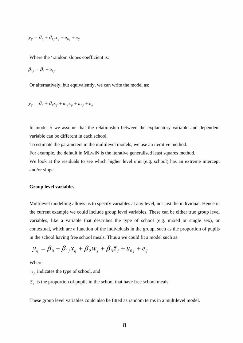
For the x variable, we begin with the most basic variable. A constant (CONS). This allows us to

assess the extent of variation in NORMEXAM at the pupil and school levels. This is model 3 on

page 11 as specified in the theory section above and you can see the equations below. Click on

the estimates button to make the full model appear in your equations window. Items in blue are

to be estimated via an iterative process. When these estimates converge as the procedure iterates

they turn green. We can see the values by clicking on the estimates button again. The NAME

and SUBS buttons are also useful for seeing the names of variables and subscripts on the output.

15

16

17

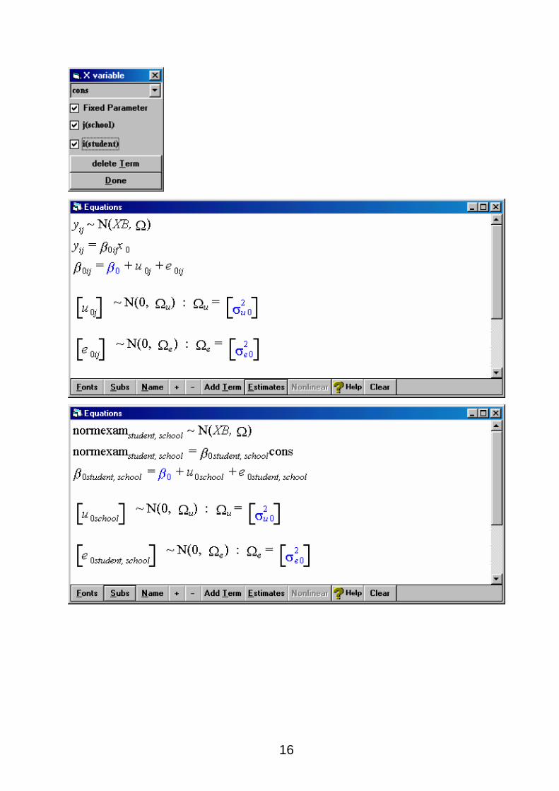
Now click on START in the top left of the main Mlwin window to make the model estimation

process begin.

** NB save the worksheet before continuing! **

In the equations window above, the green, converged, estimates are shown after a few iterations,

and we can see that the school level variance component is 0.169 and the pupil level estimate is

0.848. Hence the intra school correlation is 0.169 / (0.169+0.848) = 0.166. This suggests that

around 16.6% of the variation in NORM exam is at the school level and the remaining variation

is at the pupil level. However, so far we have not allowed for any explanatory variables. Let’s

try adding one in now to fit a multilevel model with random intercepts (like Model 4 in the

theory section above on p11.). To do this click the add term button.

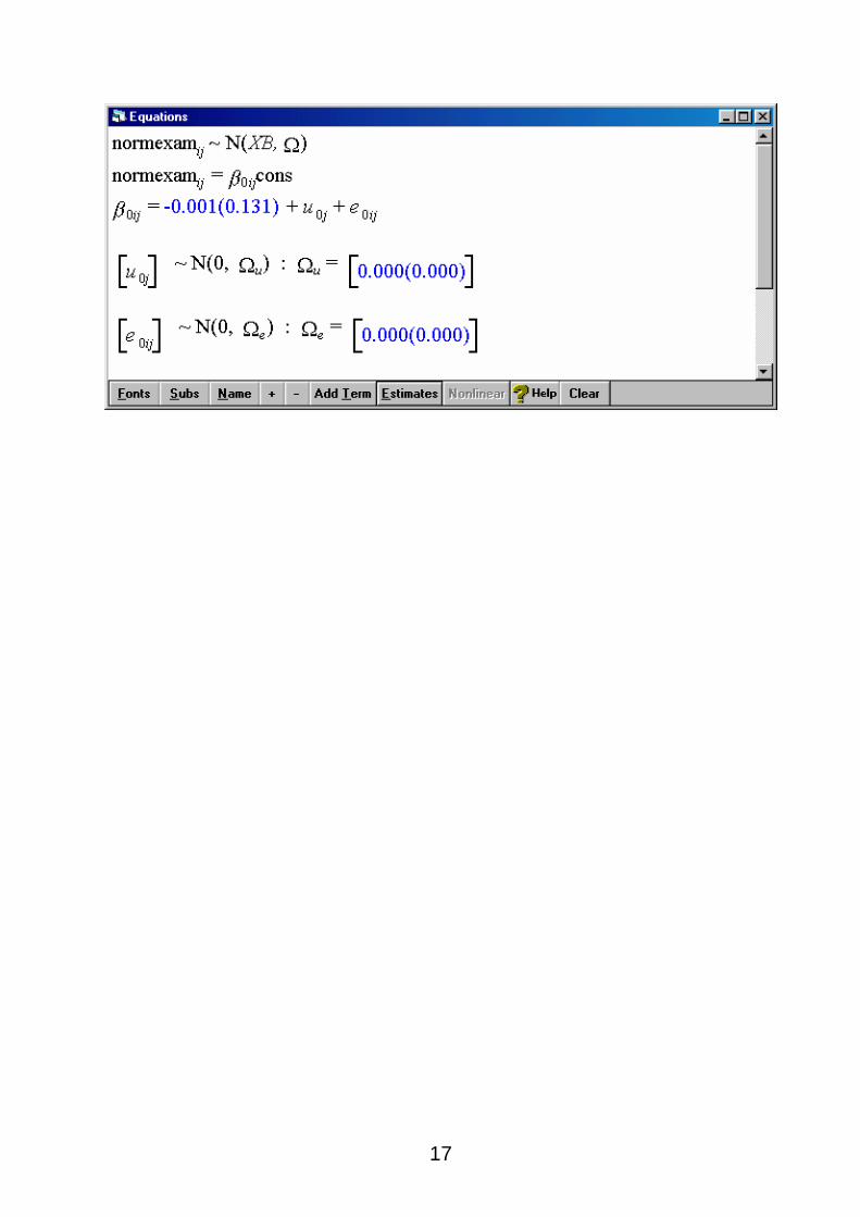
We will add in STANDLRT as an explanatory variable as shown below.

18

Click on ‘MORE’ or ‘START’ in the top left corner of the mlwin screen. Start starts the

estimation from scratch. MORE continues the estimation based on the values of those already

estimated in the previous model and may be quicker to get to the answer when you have a huge

dataset. Note also when you do have a huge dataset you can increase the size of the mlwin

worksheet via the options menu.

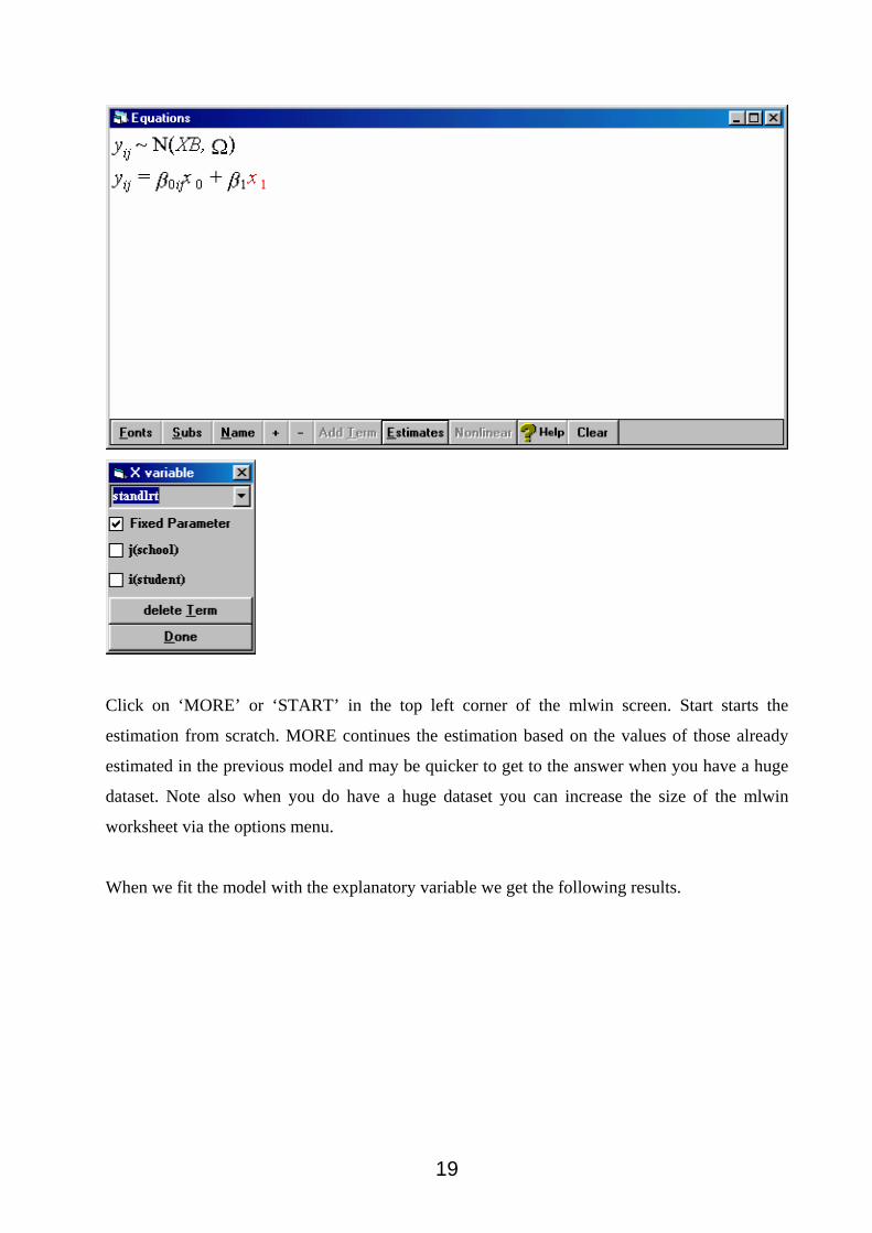
When we fit the model with the explanatory variable we get the following results.

19

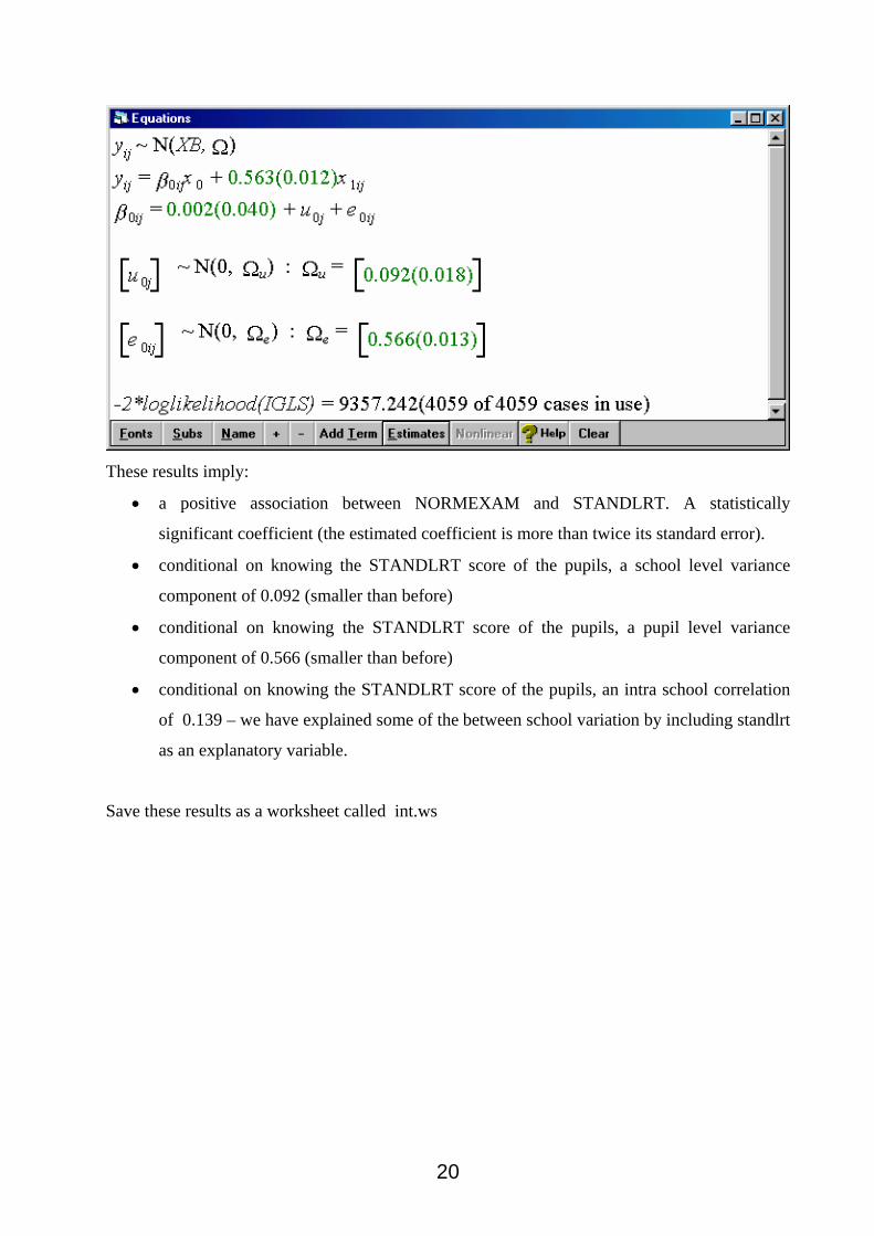
These results imply:

• a positive association between NORMEXAM and STANDLRT. A statistically

significant coefficient (the estimated coefficient is more than twice its standard error).

• conditional on knowing the STANDLRT score of the pupils, a school level variance

component of 0.092 (smaller than before)

• conditional on knowing the STANDLRT score of the pupils, a pupil level variance

component of 0.566 (smaller than before)

• conditional on knowing the STANDLRT score of the pupils, an intra school correlation

of 0.139 – we have explained some of the between school variation by including standlrt

as an explanatory variable.

Save these results as a worksheet called int.ws

20

What about random slopes? Let’s try fitting a model like (3) in the theory section above.

We see that we have now fitted quite a complicated model and all the results are statistically

significant. The positive covariance of 0.018 between intercept and slope means that schools

with steep slopes have high intercepts and schools with shallower slopes have lower intercepts.

Save these results in a worksheet called slope.ws

Graphs

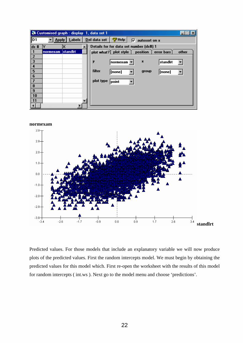
What do all these estimated models look like as graphs? We can look at them via the graphs

menu. First we will plot the data. Dependent variable vs explanatory variable. We see a general

positive association between the two variables for all 4059 pupils.

21

normexam

standlrt

Predicted values. For those models that include an explanatory variable we will now produce

plots of the predicted values. First the random intercepts model. We must begin by obtaining the

predicted values for this model which. First re-open the worksheet with the results of this model

for random intercepts ( int.ws ). Next go to the model menu and choose ‘predictions’.

22

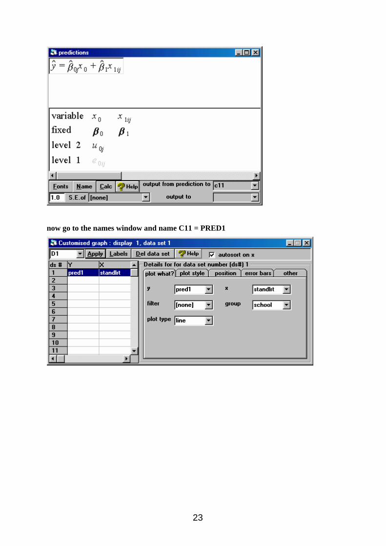
now go to the names window and name C11 = PRED1

23

pred1

standlrt

Now open the slope.ws worksheet and we can see the graph of the predicted values for the

random slopes model. Calculate the predictions as pred2

then plot them. Against the x variable (STANDLRT)

24

pred2

standlrt

25

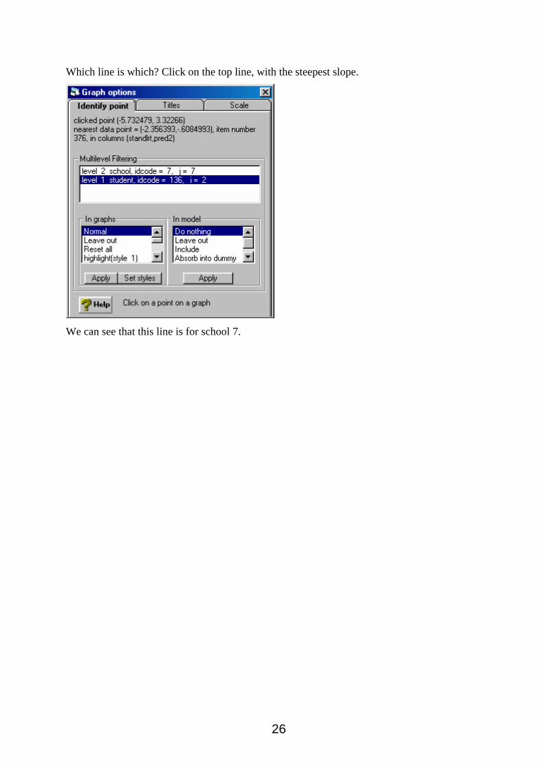
Which line is which? Click on the top line, with the steepest slope.

We can see that this line is for school 7.

26

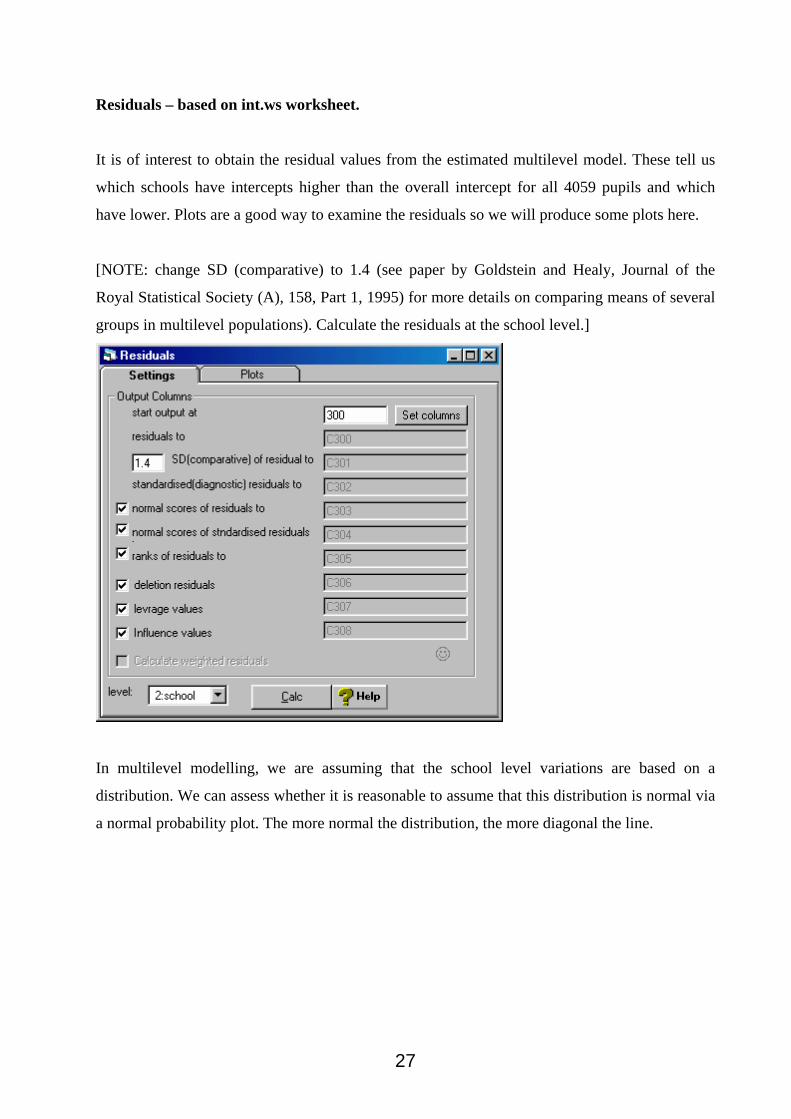
Residuals – based on int.ws worksheet.

It is of interest to obtain the residual values from the estimated multilevel model. These tell us

which schools have intercepts higher than the overall intercept for all 4059 pupils and which

have lower. Plots are a good way to examine the residuals so we will produce some plots here.

[NOTE: change SD (comparative) to 1.4 (see paper by Goldstein and Healy, Journal of the

Royal Statistical Society (A), 158, Part 1, 1995) for more details on comparing means of several

groups in multilevel populations). Calculate the residuals at the school level.]

In multilevel modelling, we are assuming that the school level variations are based on a

distribution. We can assess whether it is reasonable to assume that this distribution is normal via

a normal probability plot. The more normal the distribution, the more diagonal the line.

27

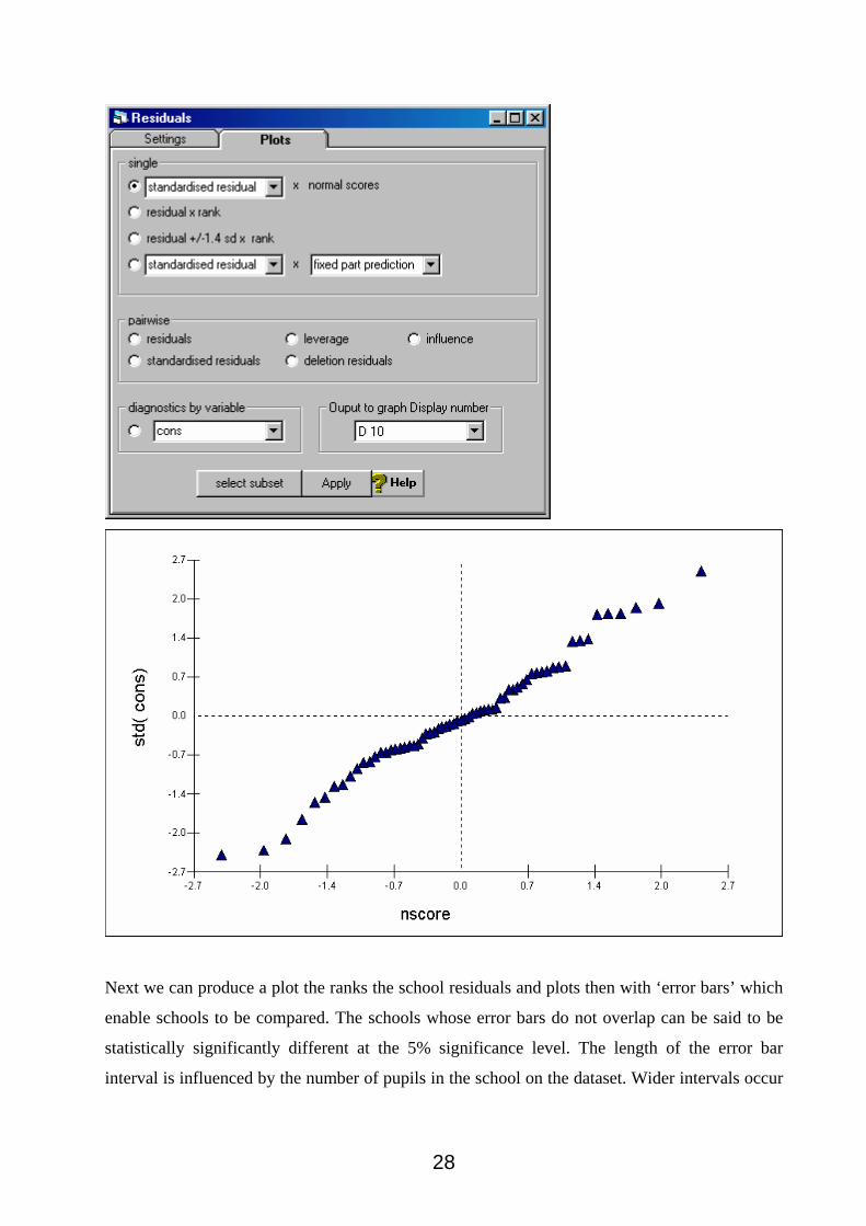
Next we can produce a plot the ranks the school residuals and plots then with ‘error bars’ which

enable schools to be compared. The schools whose error bars do not overlap can be said to be

statistically significantly different at the 5% significance level. The length of the error bar

interval is influenced by the number of pupils in the school on the dataset. Wider intervals occur

28

for schools with few pupils (in the sample) and narrower intervals for schools with more pupils

(in the sample).

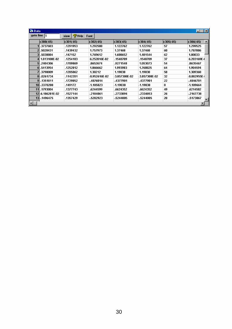
We can also see the residuals by viewing the appropriate columns of the worksheet. 65 residuals

are calculated, one for each school. We see from the data that school 1 has a residual of .37376,

ranked 57th largest of all residuals.

29

30

Section 4: Multilevel models for a binary response variable.

Introduction

This section is concerned with multilevel models that have a binary response. In many situations

the response variable is not continuous but is instead ‘binary’ (or sometimes called

‘dichotomous’ or a ‘0/1 variable’). For example, we might be interested in whether or not a

person is unemployed and would have a response variable coded 1=unemployed, 0=not

unemployed. Similarly we could be interested in whether or not a person has limiting long term

illness, and variations in long term illness by ‘place’. We might be interested in the comparative

role of place specific and personal characteristics in explaining the propensity to be unemployed.

For example, unemployment may be associated with a person’s own characteristics and (or) by

the characteristics of the place in which they live.

The example we will consider in this section is concerned with variations in unemployment for

economically active individuals aged 18 and over in the North West of England. We will first

describe the dataset and models and then try out an example using MlwiN.

The models

Model 6:

The basic (two level) multilevel model for a binary response is written as follows.

Define

ijijij epy += (6a)

where yij takes the value 0 or 1 for each individual i in group j (0=not unemployed,

1=employed), pij is the predicted probability for individual i in area j. eij is an individual level

error.

and

31

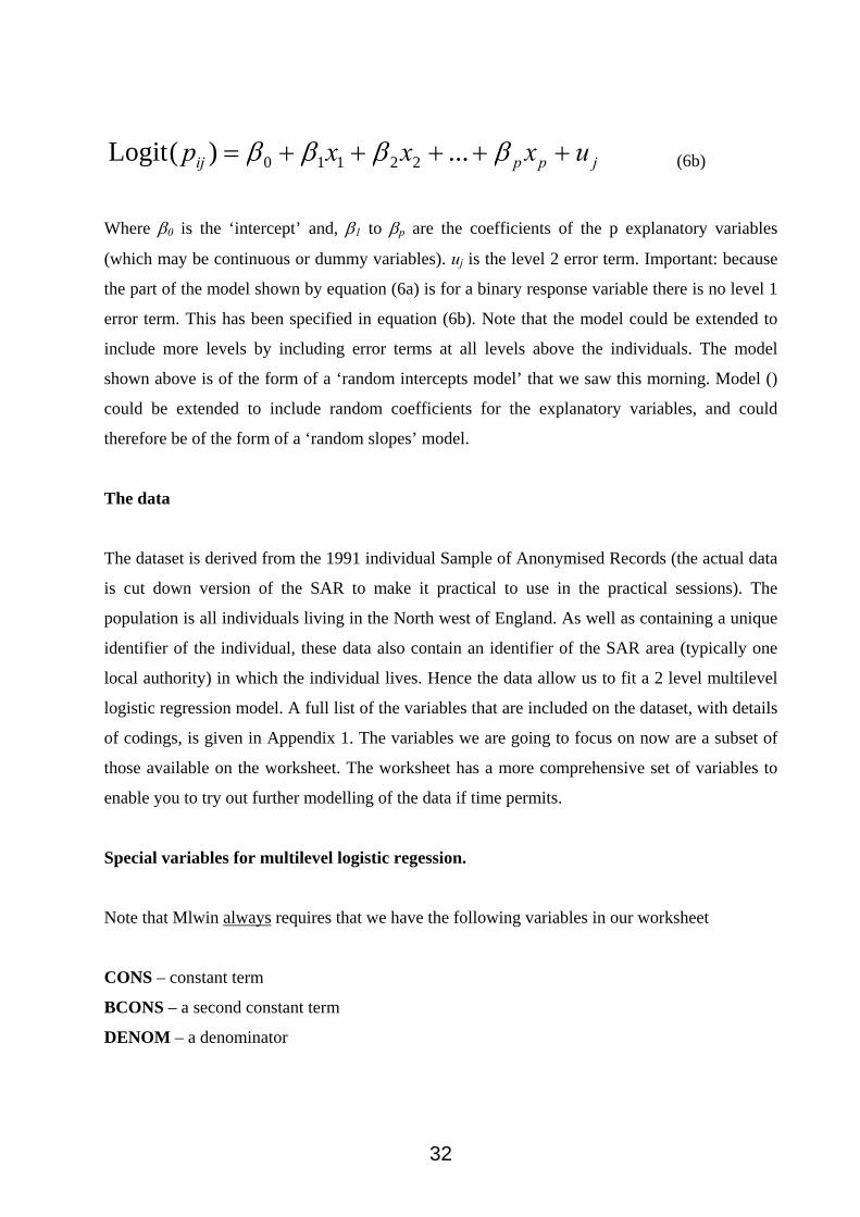
jppij uxxxp +++++= ββββ ...)(Logit 22110 (6b)

Where β0 is the ‘intercept’ and, β1 to βp are the coefficients of the p explanatory variables

(which may be continuous or dummy variables). uj is the level 2 error term. Important: because

the part of the model shown by equation (6a) is for a binary response variable there is no level 1

error term. This has been specified in equation (6b). Note that the model could be extended to

include more levels by including error terms at all levels above the individuals. The model

shown above is of the form of a ‘random intercepts model’ that we saw this morning. Model ()

could be extended to include random coefficients for the explanatory variables, and could

therefore be of the form of a ‘random slopes’ model.

The data

The dataset is derived from the 1991 individual Sample of Anonymised Records (the actual data

is cut down version of the SAR to make it practical to use in the practical sessions). The

population is all individuals living in the North west of England. As well as containing a unique

identifier of the individual, these data also contain an identifier of the SAR area (typically one

local authority) in which the individual lives. Hence the data allow us to fit a 2 level multilevel

logistic regression model. A full list of the variables that are included on the dataset, with details

of codings, is given in Appendix 1. The variables we are going to focus on now are a subset of

those available on the worksheet. The worksheet has a more comprehensive set of variables to

enable you to try out further modelling of the data if time permits.

Special variables for multilevel logistic regession.

Note that Mlwin always requires that we have the following variables in our worksheet

CONS – constant term

BCONS – a second constant term

DENOM – a denominator

32

If you look back at the model for multilevel logistic regression, you can see that the model is not

like the multilevel model for a normal response. Instead of directly modelling the y variable, as

we did for a continuous response, in multilevel logistic regression, we first re-write the response

variable as a predicted probability and an error term (the individual level error) and then we

model the predicted probability

Hence we write down a multilevel model that contains error terms for all levels above the

individual, but not the individual level, and allow for the individual term separately through the

bcons variable. The cons term is used to allow for the errors above the individual level. Hence

both cons and bcons are used in the model.

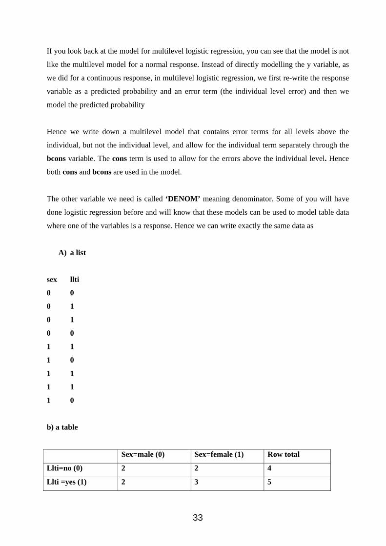
The other variable we need is called ‘DENOM’ meaning denominator. Some of you will have

done logistic regression before and will know that these models can be used to model table data

where one of the variables is a response. Hence we can write exactly the same data as

A) a list

sex llti

0 0

0 1

0 1

0 0

1 1

1 0

1 1

1 1

1 0

b) a table

Sex=male (0) Sex=female (1) Row total

Llti=no (0) 2 2 4

Llti =yes (1) 2 3 5

33

Column Total 4 5 9

For the list data DENOM is always 1 because we are looking at each person and at a time and

we have a variable whether or not they have limiting long term illness, we also record their sex

as 0 =male, 1=female. For the table data we take all the males and see how many of them have

llti, hence for the table data, for males the denom is 4 and for females the denom is 5. Both

forms of data can be modelled in mlwin. List data has greater flexibility but takes up more space

than table data. Table data has less flexibility but takes up less space than list data. In this

practical we will use list data as it is easier to explain the methods for this practical and it makes

the dataset more flexible As we are using list data here, denom is always = 1.

If all of this is a little confusing, the good news is that we always use these variables in Mlwin

for logistic multilevel modelling and the denominator must always be called DENOM. So it is

sufficient to simply include them on your M|LwiN worksheet and not get too involved in the

technicalities!

34

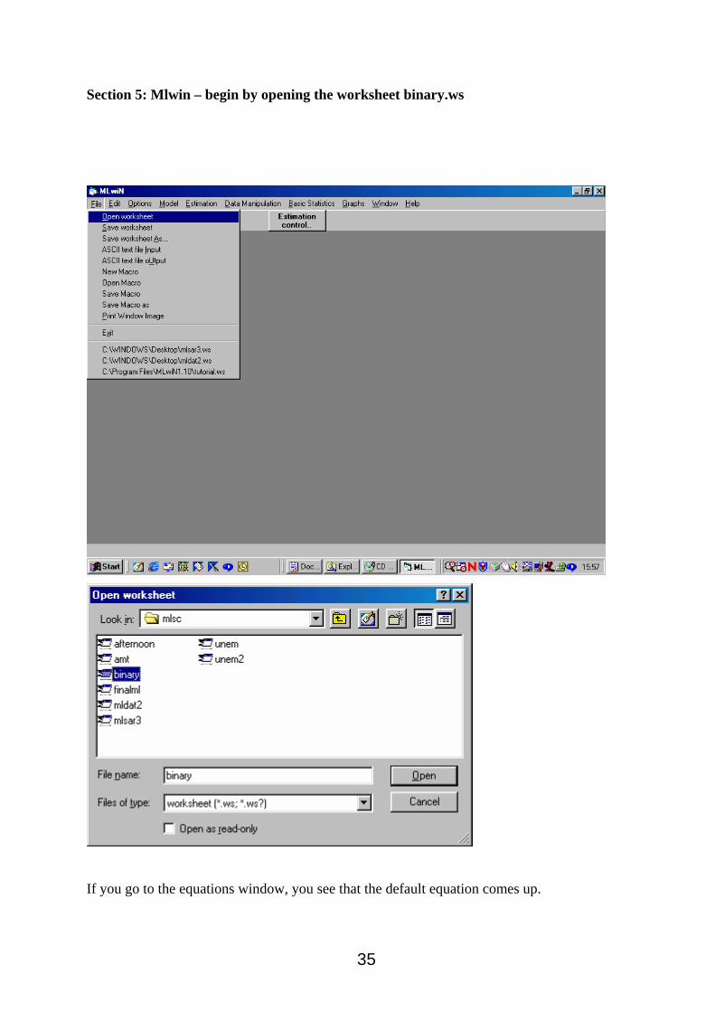
Section 5: Mlwin – begin by opening the worksheet binary.ws

If you go to the equations window, you see that the default equation comes up.

35

Specify unemployment as the y variable with areap (SAR areas) at level 2 and individuals at

level 1.

Choose the binomial distribution by clicking on the ‘normal’ N and changing it. Binomial is

used for logistic regression.

36

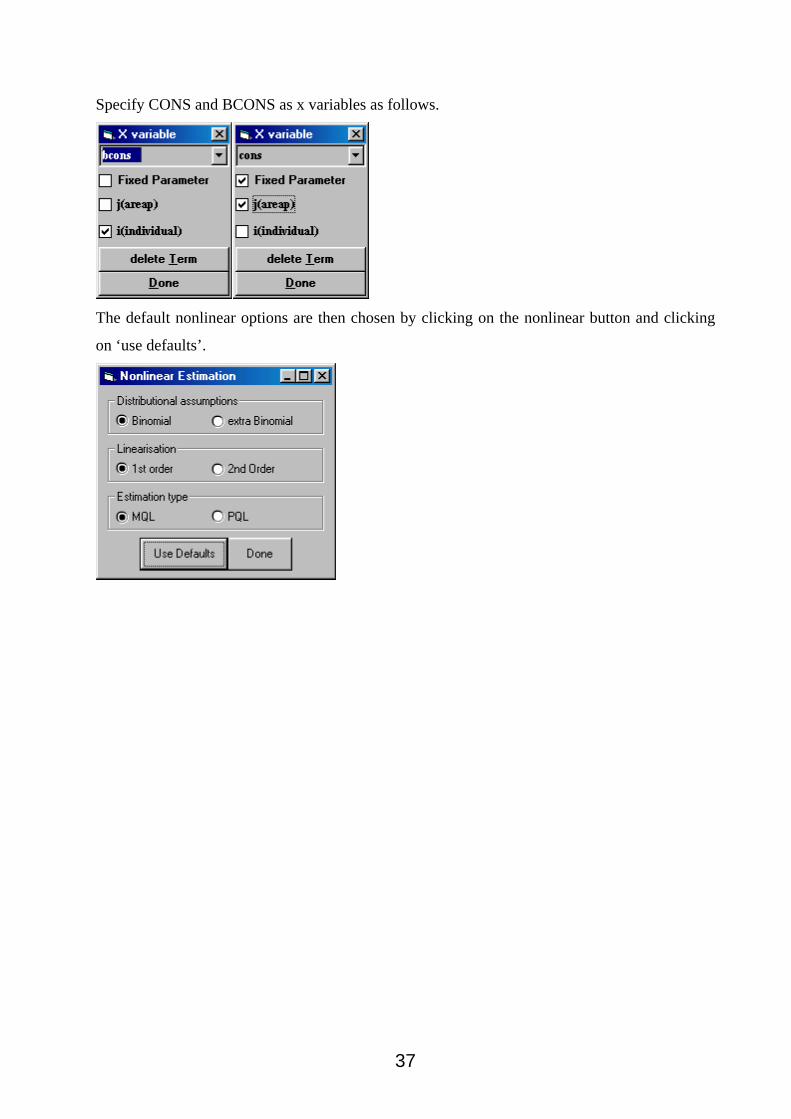
Specify CONS and BCONS as x variables as follows.

The default nonlinear options are then chosen by clicking on the nonlinear button and clicking

on ‘use defaults’.

37

We begin by fitting a variance components model. Note that it is much much harder to calculate

intra class correlations for a binary response multilevel model. For a discussion of methods see

Goldstein, Brown and Rasbash (2000).

Next we add in an age explanatory variable

38

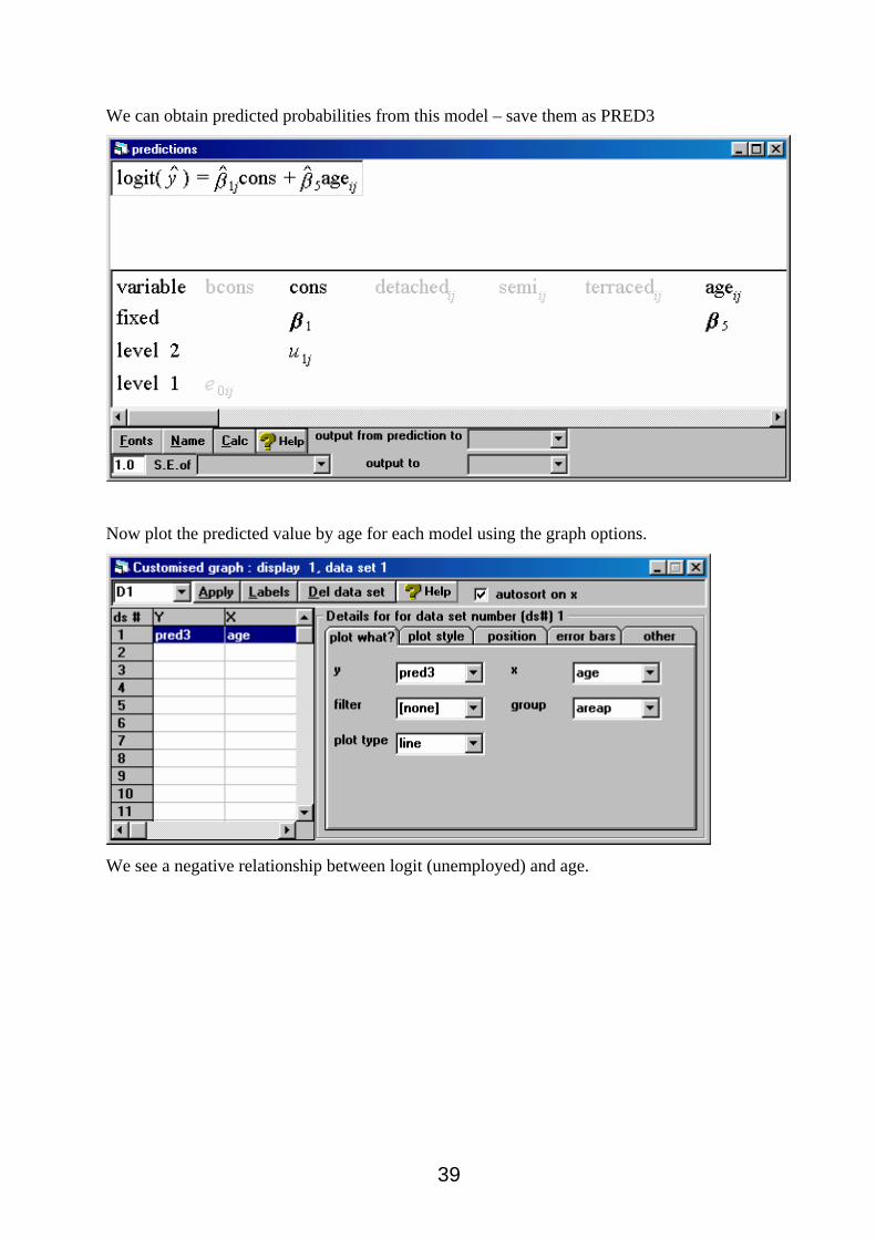
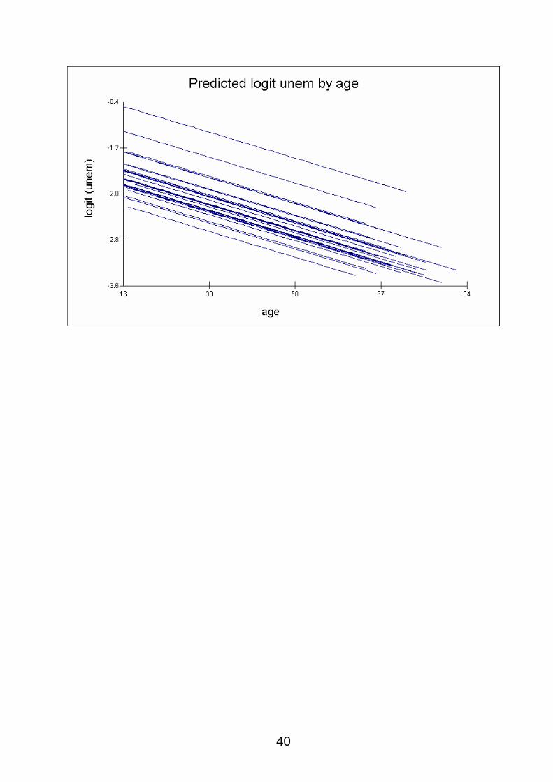
We can obtain predicted probabilities from this model – save them as PRED3

Now plot the predicted value by age for each model using the graph options.

We see a negative relationship between logit (unemployed) and age.

39

40

We could also fit a random slopes model.

The slope terms are not statistically significant.

We will now add some more explanatory variables to the model. A quick way to do this is via

the estimate tables window, first choose this from the model menu and then click on the

plus/minus button.

41

The current variables in the model are indicated with a cross.

We can add in some dummy variables for the 10 ethnic groups. We need 9 dummy variables.

When we run the model we can compare the ethnic groups. ‘white’ is the baseline ethnic group.

42

Note that we can choose more sophisticated estimation procedures for the model via the

nonlinear options window. These often give results very similar to the default, but in some

circumstances PQL estimation may be preferable to MQL and it is useful to see that different

kinds of estimation are available.

43

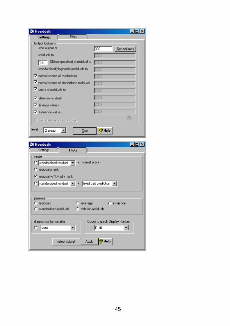
Residuals.

We can calculate and plot residuals for the model with no explanatory variables to see the extent

of variation in unemployment in areas of the North West.

We calculate the residuals as before (but note: these residuals are on the logit scale).

44

45

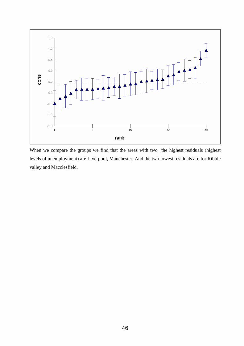
When we compare the groups we find that the areas with two the highest residuals (highest

levels of unemployment) are Liverpool, Manchester, And the two lowest residuals are for Ribble

valley and Macclesfield.

46

If we fit a more sophisticated model, which includes details of ethnic group, housing tenure and

age we can again calculate and plot the residuals from this model.

47

We see that the two highest residuals are still Liverpool and Manchester, and the lowest two

residuals are Ribble valley and Warrington. However, notice that the range of the residuals has

reduced, compared with the model with no explanatory variables. Hence we have explained

some of the variation by including information on age, ethnic group and housing.

Section 6: further topics.

ASCII data.

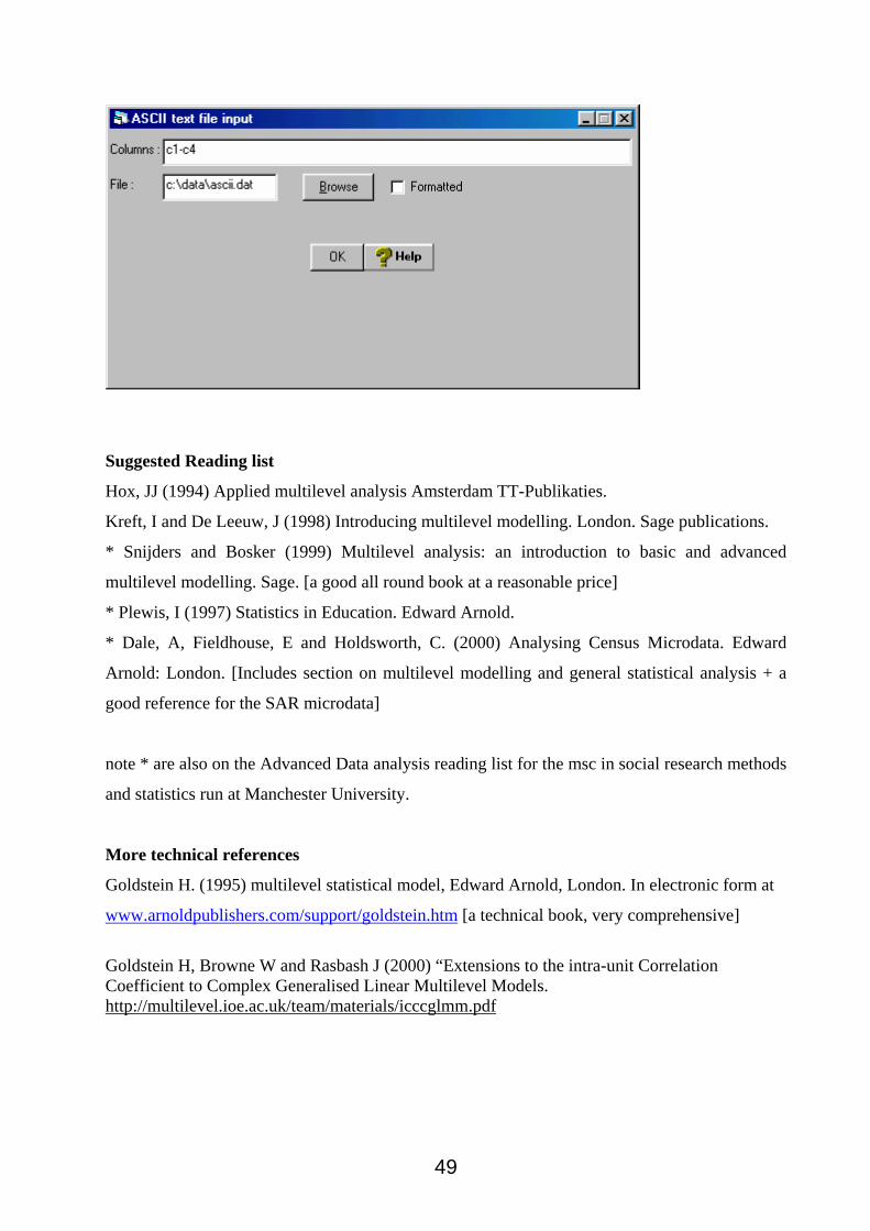
Data should be in the following format for use with ml win. We can save it as tab delimited ascii

data. E.g is spss tab delimited ascii. If possible sort the data by area (or whatever the groups are)

prior to inputting to mlwin; but note you can sort data in mlwin if necessary). We can read in

fixed format data, or as data in columns (as shown below). Data in columns is easiest read in and

the procedure will be described here. For more details of reading in data see the Mlwin User

guide.

Format of data: assume this is c:\data\ascii.dat Area person blood pressure age

1 1 100 34 1 2 120 45 1 3 150 60 1 4 107 31 1 5 125 37 1 6 144 58 2 1 102 33 2 2 99 21 2 3 102 45 2 4 101 36 2 5 123 72 2 6 112 56 2 7 101 55 2 8 102 24 We would read this data by going to the file menu and choosing ascii text file input and

then specifying that we have 4 columns of data as follows:

48

Suggested Reading list

Hox, JJ (1994) Applied multilevel analysis Amsterdam TT-Publikaties.

Kreft, I and De Leeuw, J (1998) Introducing multilevel modelling. London. Sage publications.

* Snijders and Bosker (1999) Multilevel analysis: an introduction to basic and advanced

multilevel modelling. Sage. [a good all round book at a reasonable price]

* Plewis, I (1997) Statistics in Education. Edward Arnold.

* Dale, A, Fieldhouse, E and Holdsworth, C. (2000) Analysing Census Microdata. Edward

Arnold: London. [Includes section on multilevel modelling and general statistical analysis + a

good reference for the SAR microdata]

note * are also on the Advanced Data analysis reading list for the msc in social research methods

and statistics run at Manchester University.

More technical references

Goldstein H. (1995) multilevel statistical model, Edward Arnold, London. In electronic form at

www.arnoldpublishers.com/support/goldstein.htm [a technical book, very comprehensive]

Goldstein H, Browne W and Rasbash J (2000) “Extensions to the intra-unit Correlation Coefficient to Complex Generalised Linear Multilevel Models. http://multilevel.ioe.ac.uk/team/materials/icccglmm.pdf

49

Websites:

http://multilevel.ioe.ac.uk

Includes details of current developments and publications in multilevel modelling.

Other examples of work with multilevel models. www.ioe.ac.uk/multilevel/publications

These notes are by Mark Tranmer, 2004.

50

Assignment – FOR 5 CREDITS

(nb: people doing Advanced Data Analysis by Short Course do not need to do this

assignment.)

1. Briefly describe a multilevel population indicating the units of interest at each level.

2. Write down a (two level) multilevel model for a response (i.e dependent) variable of

interest that is:

(i) a continuous variable – random intercepts model

(ii) a continuous variable – random slopes model

(iii) a binary variable

3. The following results were obtained when a variance components model was fitted in

MLwiN The population has two levels, with individuals, indexed by i, living in areas,

indexed by j, for a variable with a continuous response. Write down the variance

components estimates for the individual level and the area level. Calculate and interpret

the intra-area correlation.

[ ] [ ]

[ ] [ ])018.0(705.0:),0(~

)029.0(133.0:),0(~

)069.0(653.0

~

000

00

=ΩΩ

=ΩΩ

++=

=

Ω

eeoij

uuoj

ijjj

jij

ij

Ne

Nu

eu

xy

)Ν(XΒ,y

β

β

Hand in all work to Margaret Martin, Room NG22 Dover Street Building ground floor.

Tel 0161 275 4589 email margaret.martin@man.ac.uk

Assignment deadlines: for those people taking the assessed part of the course, for credits.

The deadline is Friday March 26th 2004.

51

52

Appendix 1: details of binary.ws variables

Name Details

AREAP SAR AREA

AGE AGE OF INDIVIDUAL

LTILL LIMITING LONG TERM ILLNESS: 0=NO 1=YES

SEX SEX OF INDIVIDUAL 0=MALE, 1=FEMALE

DENSITY MORE THAN 1 PERSON PER ROOM 0=NO 1=YES

INDIVIDUAL INDIVIDUAL ID

CONS CONSTANT TERM

BCONS CONSTANT TERM

UKBORN BORN UK 0=NO 1=YES

UNEM UNEMPLOYED 0=NO 1=YES

C-HEAT CENTRAL HEATING IN HOME 0=NO, 1=YES

DENOM DENOMINATOR VARIABLE (ALWAYS=1 HERE)

WHITE WHITE ETHNIC GROUP 0=NO 1=YES

BLACKC BLACK CARIBBEAN 0=NO, 1=YES

BLACKAF BLACK AFRICAN 0=NO, 1=YES

BLACKOTH BLACK OTHER 0=NO, 1=YES

INDIAN INDIAN 0=NO, 1=YES

PAKISTANI PAKISTANI 0=NO, 1=YES

BANGLAD BANGLADESHI 0=NO, 1=YES

CHINESE CHINESE 0=NO, 1=YES

OTHERAS OTHER ASIAN 0=NO, 1=YES

OTHER OTHER ETHNIC GROUP 0=NO, 1=YES

DETACHED LIVES IN DETACHED HOUSE 0=NO, 1=YES

SEMI LIVES IN SEMI DETACHED HOUSE 0=NO, 1=YES

TERRACED LIVES IN TERRACED HOUSE 0=NO, 1=YES

FLAT/FLATLET LIVES IN FLATFLATLET 0=NO, 1=YES

OTHERHTYPE 0=YES 1=NO

OO OWNER OCCUPIER O=NO, 1=YES

RENT PRIV RENT PRIVATELY 0=NO, 1=YES

RENT LA RENT FROM LOCAL AUTHORITY 0=NO, 1=YES

RENT OTHER RENT FROM SOMEWHERE ELSE 0=NO, 1=YES

53