Multilevel linear models: the basicsvulstats.ucsd.edu/pdf/Gelman.ch-12.basic-multilevel-models.pdfMultilevel linear models: the basics Multilevel modeling can be thought of in two

CHAPTER 12

Multilevel linear models: the basics

Multilevel modeling can be thought of in two equivalent ways:• We can think of a generalization of linear regression, where intercepts, and possi-

bly slopes, are allowed to vary by group. For example, starting with a regressionmodel with one predictor, yi = ! + "xi + #i, we can generalize to the varying-intercept model, yi = !j[i] + "xi + #i, and the varying-intercept, varying-slopemodel, yi = !j[i] + "j[i]xi + #i (see Figure 11.1 on page 238).

• Equivalently, we can think of multilevel modeling as a regression that includes acategorical input variable representing group membership. From this perspective,the group index is a factor with J levels, corresponding to J predictors in theregression model (or 2J if they are interacted with a predictor x in a varying-intercept, varying-slope model; or 3J if they are interacted with two predictorsX(1), X(2); and so forth).

In either case, J!1 linear predictors are added to the model (or, to put it anotherway, the constant term in the regression is replaced by J separate intercept terms).The crucial multilevel modeling step is that these J coe!cients are then themselvesgiven a model (most simply, a common distribution for the J parameters !j or,more generally, a regression model for the !j ’s given group-level predictors). Thegroup-level model is estimated simultaneously with the data-level regression of y.

This chapter introduces multilevel linear regression step by step. We begin inSection 12.2 by characterizing multilevel modeling as a compromise between twoextremes: complete pooling, in which the group indicators are not included in themodel, and no pooling, in which separate models are fit within each group. Afterlaying out some notational di!culties in Section 12.5, we discuss in Section 12.6 thedi"erent roles of the individual- and group-level regressions. Chapter 13 continueswith more complex multilevel structures.

12.1 Notation

We briefly review the notation for classical regression and then outline how it canbe generalized for multilevel models. As we illustrate in the examples, however, nosingle notation is appropriate for all problems. We use the following notation forclassical regression:• Units i = 1, . . . , n. By units, we mean the smallest items of measurement.• Outcome measurements y = (y1, . . . , yn). These are the unit-level data being

modeled.• Regression predictors are represented by an n " k matrix X , so that the vector

of predicted values is y = X", where y and " are column vectors of length nand k, respectively. We include in X the constant term (unless it is explicitlyexcluded from the model), so that the first column of X is all 1’s. We usuallylabel the coe!cients as "0, . . . , "k!1, but sometimes we index from 1 to k.

• For each individual unit i, we denote its row vector of predictors as Xi. Thus,yi = Xi" is the prediction for unit i.

251

252 MULTILEVEL LINEAR MODELS: THE BASICS

• For each predictor !, we label the (!+1)st column of X as X(!) (assuming thatX(0) is a column of 1’s).

• Any information contained in the unit labels i should be coded in the regres-sion inputs. For example, if i = 1, . . . , n represents the order in which personsi enrolled in a study, we should create a time variable ti and, for example, in-clude it in the matrix X of regression predictors. Or, more generally, considertransformations and interactions of this new input variable.

For multilevel models, we label:• Groups j = 1, . . . , J . This works for a single level of grouping (for example,

students within schools, or persons within states).• We occasionally use k = 1, . . . , K for a second level of grouping (for exam-

ple, students within schools within districts; or, for a non-nested example, testresponses that can be characterized by person or by item). In any particularexample, we have to distinguish this k from the number of predictors in X . Formore complicated examples we develop idiosyncratic notation as appropriate.

• Index variables j[i] code group membership. For example, if j[35] = 4, then the35th unit in the data (i = 35) belongs to group 4.

• Coe!cients are sometimes written as a vector ", sometimes as #, " (as in Figure11.1 on page 238), with group-level regression coe!cients typically called $.

• We make our R and Bugs code more readable by typing #, ", $ as a,b,g.• We write the varying-intercept model with one additional predictor as yi =

#j[i]+"xi+%i or yi ! N(#j[i]+"xi, &2y). Similarly, the varying-intercept, varying-

slope model is yi = #j[i] + "j[i]xi + %i or yi ! N(#j[i] + "j[i]xi, &2y).

• With multiple predictors, we write yi = XiB + %i, or yi ! N(XiB, &2y). B is

a matrix of coe!cients that can be modeled using a general varying-intercept,varying-slope model (as discussed in the next chapter).

• Standard deviation is &y for data-level errors and &", &# , and so forth, for group-level errors.

• Group-level predictors are represented by a matrix U with J rows, for example,in the group-level model, #j ! N(Uj$, &2

"). When there is a single group-levelpredictor, we label it as lowercase u.

12.2 Partial pooling with no predictors

As noted in Section 1.3, multilevel regression can be thought of as a method forcompromising between the two extremes of excluding a categorical predictor froma model (complete pooling), or estimating separate models within each level of thecategorical predictor (no pooling).

Complete-pooling and no-pooling estimates of county radon levels

We illustrate with the home radon example, which we introduced in Section 1.2 andshall use throughout this chapter. Consider the goal of estimating the distribution ofradon levels of the houses within each of the 85 counties in Minnesota.1 This seems1 Radon levels are always positive, and it is reasonable to suppose that e!ects will be multiplica-

tive; hence it is appropriate to model the data on the logarithmic scale (see Section 4.4). Forsome purposes, though, such as estimating total cancer risk, it makes sense to estimate averageson the original, unlogged scale; we can obtain these inferences using simulation, as discussedat the end of Section 12.8.

PARTIAL POOLING WITH NO PREDICTORS 253

!"#$""%&'( )*%+&%,-,%#."/,%

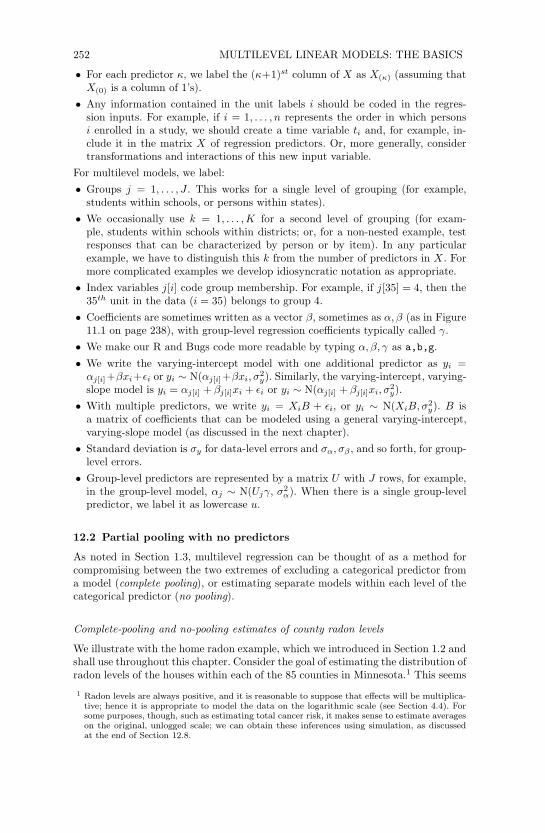
Figure 12.1 Estimates ± standard errors for the average log radon levels in Minnesotacounties plotted versus the (jittered) number of observations in the county: (a) no-poolinganalysis, (b) multilevel (partial pooling) analysis, in both cases with no house-level orcounty-level predictors. The counties with fewer measurements have more variable esti-mates and larger higher standard errors. The horizontal line in each plot represents anestimate of the average radon level across all counties. The left plot illustrates a problemwith the no-pooling analysis: it systematically causes us to think that certain counties aremore extreme, just because they have smaller sample sizes.

simple enough. One estimate would be the average that completely pools dataacross all counties. This ignores variation among counties in radon levels, however,so perhaps a better option would be simply to use the average log radon level ineach county. Figure 12.1a plots these averages against the number of observationsin each county.

Whereas complete pooling ignores variation between counties, the no-poolinganalysis overstates it. To put it another way, the no-pooling analysis overfits thedata within each county. To see this, consider Lac Qui Parle County (circled in theplot), which has the highest average radon level of all 85 counties in Minnesota.This average, however, is estimated using only two data points. Lac Qui Parle mayvery well be a high-radon county, but do we really believe it is that high? Maybe,but probably not: given the variability in the data we would not have much trustin an estimate based on only two measurements.

To put it another way, looking at all the counties together: the estimates fromthe no-pooling model overstate the variation among counties and tend to make theindividual counties look more di!erent than they actually are.

Partial-pooling estimates from a multilevel model

The multilevel estimates of these averages, displayed in Figure 12.1b, represent acompromise between these two extremes. The goal of estimation is the average logradon level !j among all the houses in county j, for which all we have availableare a random sample of size nj . For this simple scenario with no predictors, themultilevel estimate for a given county j can be approximated as a weighted averageof the mean of the observations in the county (the unpooled estimate, yj) and themean over all counties (the completely pooled estimate, yall):

!multilevelj !

nj

!2yyj + 1

!2!yall

nj

!2y

+ 1!2

!

, (12.1)


where nj is the number of measured houses in county j, !2y is the within-county

variance in log radon measurements, and !2! is the variance among the average

log radon levels of the di!erent counties. We could also allow the within-countyvariance to vary by county (in which case !y would be replaced by !y j in thepreceding formula) but for simplicity we assume it is constant.

The weighted average (12.1) reflects the relative amount of information availableabout the individual county, on one hand, and the average of all the counties, onthe other:• Averages from counties with smaller sample sizes carry less information, and the

weighting pulls the multilevel estimates closer to the overall state average. In thelimit, if nj = 0, the multilevel estimate is simply the overall average, yall.

• Averages from counties with larger sample sizes carry more information, and thecorresponding multilevel estimates are close to the county averages. In the limitas nj ! ", the multilevel estimate is simply the county average, yj .

• In intermediate cases, the multilevel estimate lies between the two extremes.To actually apply (12.1), we need estimates of the variation within and betweencounties. In practice, we estimate these variance parameters together with the "j ’s,either with an approximate program such as lmer() (see Section 12.4) or usingfully Bayesian inference, as implemented in Bugs and described in Part 2B of thisbook. For now, we present inferences (as in Figure 12.1) without dwelling on thedetails of estimation.

12.3 Partial pooling with predictors

The same principle of finding a compromise between the extremes of completepooling and no pooling applies for more general models. This section considerspartial pooling for a model with unit-level predictors. In this scenario, no poolingmight refer to fitting a separate regression model within each group. However, a lessextreme and more common option that we also sometimes refer to as “no pooling”is a model that includes group indicators and estimates the model classically.2

As we move on to more complicated models, we present estimates graphicallybut do not continue with formulas of the form (12.1). However, the general prin-ciple remains that multilevel models compromise between pooled and unpooledestimates, with the relative weights determined by the sample size in the group andthe variation within and between groups.

Complete-pooling and no-pooling analyses for the radon data, with predictors

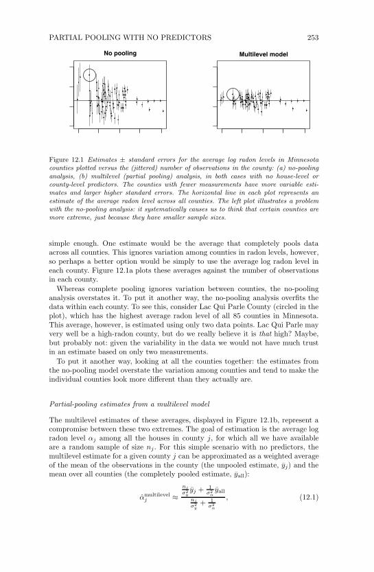
Continuing with the radon data, Figure 12.2 shows the logarithm of the home radonmeasurement versus floor of measurement3 for houses sampled from eight of the 85counties in Minnesota. (We fit our model to the data from all 85 counties, includinga total of 919 measurements, but to save space we display the data and estimatesfor a selection of eight counties, chosen to capture a range of the sample sizes inthe survey.)

In each graph of Figure 12.2, the dashed line shows the linear regression of log

2 This version of “no pooling” does not pool the estimates for the intercepts—the parameterswe focus on in the current discussion—but it does completely pool estimates for any slopecoe!cients (they are forced to have the same value across all groups) and also assumes theresidual variance is the same within each group.

3 Measurements were taken in the lowest living area of each house, with basement coded as 0and first floor coded as 1.

PARTIAL POOLING WITH PREDICTORS 255

!"#$%&'$(")!* "'+,'- ,..#/'#/'-0 1.&0!"2

#!"3 2+*")-2 )"42*3 2+$!.&'2

Figure 12.2 Complete-pooling (dashed lines, y = ! + "x) and no-pooling (solid lines,y = !j +"x) regressions fit to radon data from the 85 counties in Minnesota, and displayedfor eight of the counties. The estimated slopes " di!er slightly for the two models, but hereour focus is on the intercepts.

radon, given the floor of measurement, using a model that pools all counties together(so the same line appears in all eight plots), and the solid line shows the no-poolingregressions, obtained by including county indicators in the regression (with theconstant term removed to avoid collinearity; we also could have kept the constantterm and included indicators for all but one of the counties). We can write thecomplete-pooling regression as yi = ! + "xi + #i and the no-pooling regression asyi = !j[i] + "xi + #i, where j[i] is the county corresponding to house i. The solidlines then plot y = ! + "x from the complete-pooling model, and the dashed linesshow y = !j + "x, for j = 1, . . . , 8, from the no-pooling model.

Here is the complete-pooling regression for the radon data:

R outputlm(formula = y ~ x)coef.est coef.se

(Intercept) 1.33 0.03x -0.61 0.07n = 919, k = 2residual sd = 0.82

To fit the no-pooling model in R, we include the county index (a variable namedcounty that takes on values between 1 and 85) as a factor in the regression—thus,predictors for the 85 di!erent counties. We add “!1” to the regression formula toremove the constant term, so that all 85 counties are included. Otherwise, R woulduse county 1 as a baseline.

R outputlm(formula = y ~ x + factor(county) - 1)coef.est coef.sd

x -0.72 0.07factor(county)1 0.84 0.38factor(county)2 0.87 0.10. . .factor(county)85 1.19 0.53n = 919, k = 86residual sd = 0.76

The estimated slopes " di!er slightly for the two regressions. The no-poolingmodel includes county indicators, which can change the estimated coe"cient forx, if the proportion of houses with basements varies among counties. This is just


!

!

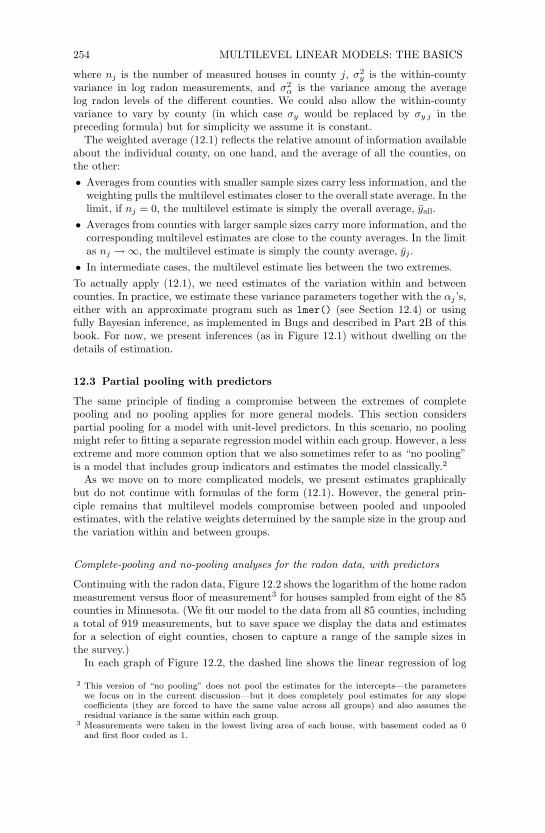
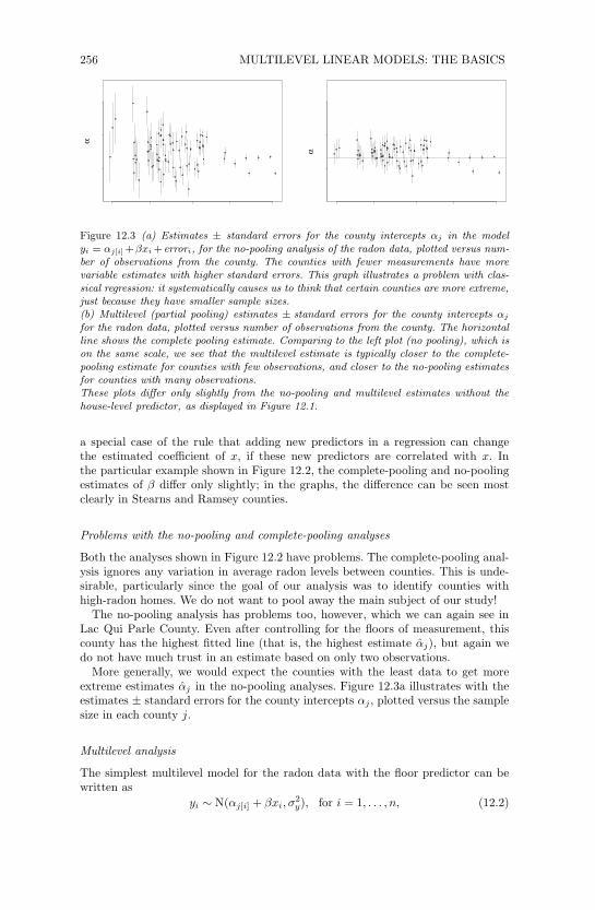
Figure 12.3 (a) Estimates ± standard errors for the county intercepts !j in the modelyi = !j[i] +"xi +errori, for the no-pooling analysis of the radon data, plotted versus num-ber of observations from the county. The counties with fewer measurements have morevariable estimates with higher standard errors. This graph illustrates a problem with clas-sical regression: it systematically causes us to think that certain counties are more extreme,just because they have smaller sample sizes.(b) Multilevel (partial pooling) estimates ± standard errors for the county intercepts !j

for the radon data, plotted versus number of observations from the county. The horizontalline shows the complete pooling estimate. Comparing to the left plot (no pooling), which ison the same scale, we see that the multilevel estimate is typically closer to the complete-pooling estimate for counties with few observations, and closer to the no-pooling estimatesfor counties with many observations.These plots di!er only slightly from the no-pooling and multilevel estimates without thehouse-level predictor, as displayed in Figure 12.1.

a special case of the rule that adding new predictors in a regression can changethe estimated coe!cient of x, if these new predictors are correlated with x. Inthe particular example shown in Figure 12.2, the complete-pooling and no-poolingestimates of ! di"er only slightly; in the graphs, the di"erence can be seen mostclearly in Stearns and Ramsey counties.

Problems with the no-pooling and complete-pooling analyses

Both the analyses shown in Figure 12.2 have problems. The complete-pooling anal-ysis ignores any variation in average radon levels between counties. This is unde-sirable, particularly since the goal of our analysis was to identify counties withhigh-radon homes. We do not want to pool away the main subject of our study!

The no-pooling analysis has problems too, however, which we can again see inLac Qui Parle County. Even after controlling for the floors of measurement, thiscounty has the highest fitted line (that is, the highest estimate "j), but again wedo not have much trust in an estimate based on only two observations.

More generally, we would expect the counties with the least data to get moreextreme estimates "j in the no-pooling analyses. Figure 12.3a illustrates with theestimates ± standard errors for the county intercepts "j , plotted versus the samplesize in each county j.

Multilevel analysis

The simplest multilevel model for the radon data with the floor predictor can bewritten as

yi ! N("j[i] + !xi, #2y), for i = 1, . . . , n, (12.2)

PARTIAL POOLING WITH PREDICTORS 257

!"#$%&'$(")!* "'+,'- ,..#/'#/'-0 1.&0!"2

#!"3 2+*")-2 )"42*3 2+$!.&'2

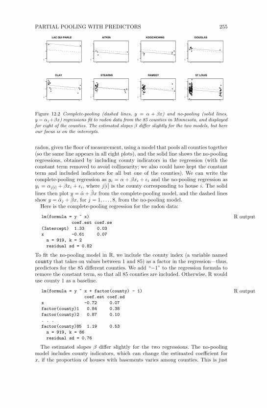
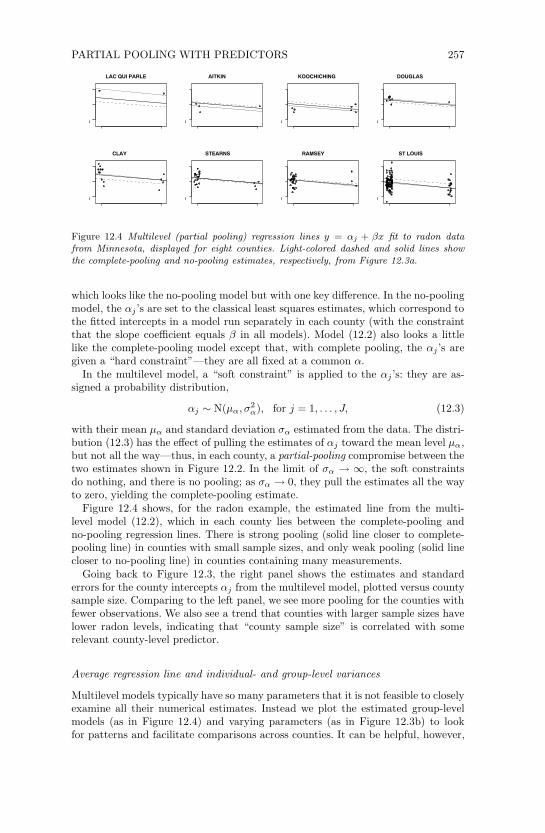
Figure 12.4 Multilevel (partial pooling) regression lines y = !j + "x fit to radon datafrom Minnesota, displayed for eight counties. Light-colored dashed and solid lines showthe complete-pooling and no-pooling estimates, respectively, from Figure 12.3a.

which looks like the no-pooling model but with one key di!erence. In the no-poolingmodel, the !j ’s are set to the classical least squares estimates, which correspond tothe fitted intercepts in a model run separately in each county (with the constraintthat the slope coe"cient equals " in all models). Model (12.2) also looks a littlelike the complete-pooling model except that, with complete pooling, the !j ’s aregiven a “hard constraint”—they are all fixed at a common !.

In the multilevel model, a “soft constraint” is applied to the !j ’s: they are as-signed a probability distribution,

!j ! N(µ!, #2!), for j = 1, . . . , J, (12.3)

with their mean µ! and standard deviation #! estimated from the data. The distri-bution (12.3) has the e!ect of pulling the estimates of !j toward the mean level µ!,but not all the way—thus, in each county, a partial-pooling compromise between thetwo estimates shown in Figure 12.2. In the limit of #! " #, the soft constraintsdo nothing, and there is no pooling; as #! " 0, they pull the estimates all the wayto zero, yielding the complete-pooling estimate.

Figure 12.4 shows, for the radon example, the estimated line from the multi-level model (12.2), which in each county lies between the complete-pooling andno-pooling regression lines. There is strong pooling (solid line closer to complete-pooling line) in counties with small sample sizes, and only weak pooling (solid linecloser to no-pooling line) in counties containing many measurements.

Going back to Figure 12.3, the right panel shows the estimates and standarderrors for the county intercepts !j from the multilevel model, plotted versus countysample size. Comparing to the left panel, we see more pooling for the counties withfewer observations. We also see a trend that counties with larger sample sizes havelower radon levels, indicating that “county sample size” is correlated with somerelevant county-level predictor.

Average regression line and individual- and group-level variances

Multilevel models typically have so many parameters that it is not feasible to closelyexamine all their numerical estimates. Instead we plot the estimated group-levelmodels (as in Figure 12.4) and varying parameters (as in Figure 12.3b) to lookfor patterns and facilitate comparisons across counties. It can be helpful, however,


to look at numerical summaries for the hyperparameters—those model parameterswithout group-level subscripts.

For example, in the radon model, the hyperparameters are estimated as µ! =1.46, ! = !0.69, "y = 0.76, and "! = 0.33. (We show the estimates in Section 12.4.)That is, the estimated average regression line for all the counties is y = 1.46!0.69x,with error standard deviations of 0.76 at the individual level and 0.33 at the countylevel. For this dataset, variation within counties (after controlling for the floor ofmeasurement) is comparable to the average di!erence between measurements inhouses with and without basements.

One way to interpret the variation between counties, "!, is to consider thevariance ratio, "2

!/"2y, which in this example is estimated at 0.332/0.762 = 0.19,

or about one-fifth. Thus, the standard deviation of average radon levels betweencounties is the same as the standard deviation of the average of 5 measurementswithin a county (that is, 0.76/

"5 = 0.33). The relative values of individual- and

group-level variances are also sometimes expressed using the intraclass correlation,"2

!/("2! + "2

y), which ranges from 0 if the grouping conveys no information to 1 ifall members of a group are identical.

In our example, the group-level model tells us that the county intercepts, #j , havean estimated mean of 1.46 and standard deviation of 0.33. (What is relevant to ourdiscussion here is the standard deviation, not the mean.) The amount of informationin this distribution is the same as that in 5 measurements within a county. To put itanother way, for a county with a sample size less than 5, there is more informationin the group-level model than in the county’s data; for a county with more than 5observations, the within-county measurements are more informative (in the senseof providing a lower-variance estimate of the county’s average radon level). As aresult, the multilevel regression line in a county is closer to the complete-poolingestimate when sample size is less than 5, and closer to the no-pooling estimate whensample size exceeds 5. We can see this in Figure 12.4: as sample size increases, themultilevel estimates move closer and closer to the no-pooling lines.

Partial pooling (shrinkage) of group coe!cients #j

Multilevel modeling partially pools the group-level parameters #j toward theirmean level, µ!. There is more pooling when the group-level standard deviation"! is small, and more smoothing for groups with fewer observations. Generaliz-ing (12.1), the multilevel-modeling estimate of #j can be expressed as a weightedaverage of the no-pooling estimate for its group (yj ! !xj) and the mean, µ!:

estimate of #j #nj

"2y

nj

"2y

+ 1"2

!

(yj ! !xj) +1

"2!

nj

"2y

+ 1"2

!

µ!. (12.4)

When actually fitting multilevel models, we do not actually use this formula; rather,we fit models using lmer() or Bugs, which automatically perform the calculations,using formulas such as (12.4) internally. Chapter 19 provides more detail on thealgorithms used to fit these models.

Classical regression as a special case

Classical regression models can be viewed as special cases of multilevel models.The limit of "! $ 0 yields the complete-pooling model, and "! $ % reduces tothe no-pooling model. Given multilevel data, we can estimate "!. Therefore we

QUICKLY FITTING MULTILEVEL MODELS IN R 259

see no reason (except for convenience) to accept estimates that arbitrarily set thisparameter to one of these two extreme values.

12.4 Quickly fitting multilevel models in R

We fit most of the multilevel models in this part of the book using the lmer()function, which fits linear and generalized linear models with varying coe!cients.4Part 2B of the book considers computation in more detail, including a discussionof why it can be helpful to make the extra e"ort and program models using Bugs(typically using a simpler lmer() fit as a starting point). The lmer() functionis currently part of the R package Matrix; see Appendix C for details. Here weintroduce lmer() in the context of simple varying-intercept models.

The lmer function

Varying-intercept model with no predictors. The varying intercept model with nopredictors (discussed in Section 12.2) can be fit and displayed using lmer() asfollows:

R codeM0 <- lmer (y ~ 1 + (1 | county))display (M0)

This model simply includes a constant term (the predictor “1”) and allows it tovary by county. We next move to a more interesting model including the floor ofmeasurement as an individual-level predictor.Varying-intercept model with an individual-level predictor. We shall introduce mul-tilevel fitting with model (12.2)–(12.3), the varying-intercept regression with a singlepredictor. We start with the call to lmer():

R codeM1 <- lmer (y ~ x + (1 | county))

This expression starts with the no-pooling model, “y ~ x,” and then adds “(1 |county),” which allows the intercept (the coe!cient of the predictor “1,” which isthe column of ones—the constant term in the regression) to vary by county.

We can then display a quick summary of the fit:

R codedisplay (M1)

which yields

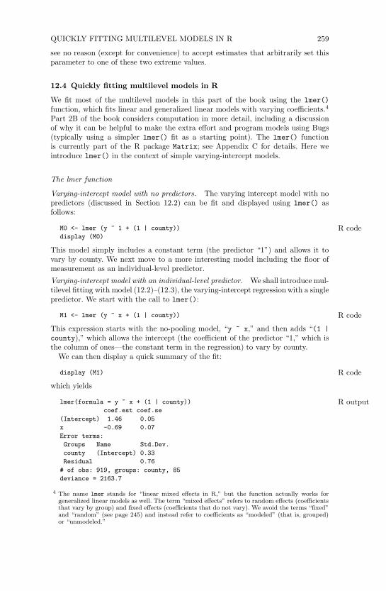
R outputlmer(formula = y ~ x + (1 | county))coef.est coef.se

(Intercept) 1.46 0.05x -0.69 0.07Error terms:Groups Name Std.Dev.county (Intercept) 0.33Residual 0.76# of obs: 919, groups: county, 85deviance = 2163.7

4 The name lmer stands for “linear mixed e!ects in R,” but the function actually works forgeneralized linear models as well. The term “mixed e!ects” refers to random e!ects (coe"cientsthat vary by group) and fixed e!ects (coe"cients that do not vary). We avoid the terms “fixed”and “random” (see page 245) and instead refer to coe"cients as “modeled” (that is, grouped)or “unmodeled.”


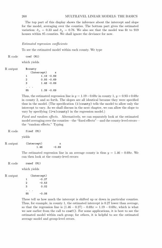
The top part of this display shows the inference about the intercept and slopefor the model, averaging over the counties. The bottom part gives the estimatedvariation: !! = 0.33 and !y = 0.76. We also see that the model was fit to 919houses within 85 counties. We shall ignore the deviance for now.

Estimated regression coe!cients

To see the estimated model within each county. We type

R code coef (M1)

which yields

R output $county(Intercept) x

1 1.19 -0.692 0.93 -0.693 1.48 -0.69. . .85 1.39 -0.69

Thus, the estimated regression line is y = 1.19!0.69x in county 1, y = 0.93+0.69xin county 2, and so forth. The slopes are all identical because they were specifiedthus in the model. (The specification (1|county) tells the model to allow only theintercept to vary. As we shall discuss in the next chapter, we can allow the slope tovary by specifying (1+x|county) in the regression model.)Fixed and random e"ects. Alternatively, we can separately look at the estimatedmodel averaging over the counties—the “fixed e!ects”—and the county-level errors—the “random e!ects.” Typing

R code fixef (M1)

yields

R output (Intercept) x1.46 -0.69

The estimated regression line in an average county is thus y = 1.46 ! 0.69x. Wecan then look at the county-level errors:

R code ranef (M1)

which yields

R output (Intercept)1 -0.272 -0.533 0.02. . .85 -0.08

These tell us how much the intercept is shifted up or down in particular counties.Thus, for example, in county 1, the estimated intercept is 0.27 lower than average,so that the regression line is (1.46 ! 0.27) ! 0.69x = 1.19 ! 0.69x, which is whatwe saw earlier from the call to coef(). For some applications, it is best to see theestimated model within each group; for others, it is helpful to see the estimatedaverage model and group-level errors.

QUICKLY FITTING MULTILEVEL MODELS IN R 261

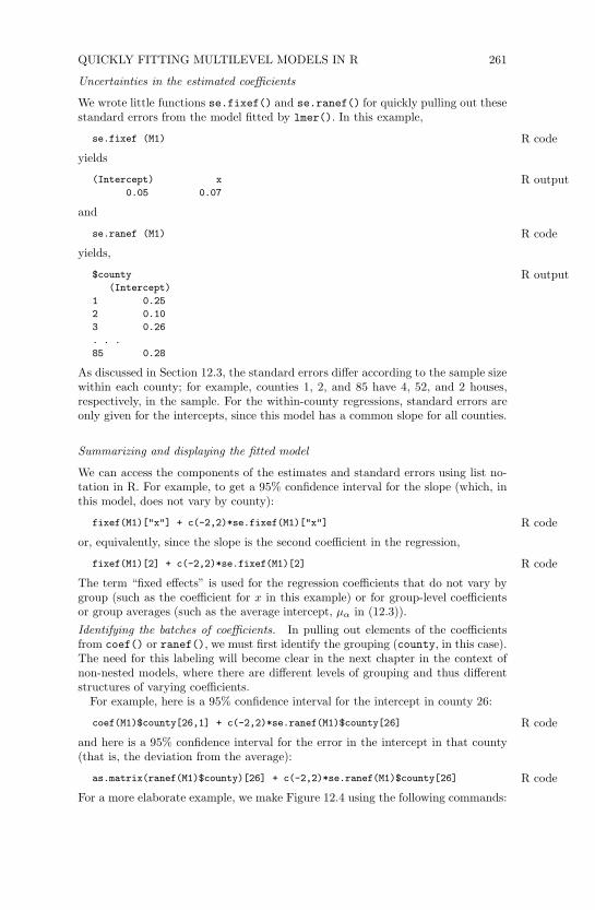
Uncertainties in the estimated coe!cients

We wrote little functions se.fixef() and se.ranef() for quickly pulling out thesestandard errors from the model fitted by lmer(). In this example,

R codese.fixef (M1)

yields

R output(Intercept) x0.05 0.07

and

R codese.ranef (M1)

yields,

R output$county(Intercept)

1 0.252 0.103 0.26. . .85 0.28

As discussed in Section 12.3, the standard errors di!er according to the sample sizewithin each county; for example, counties 1, 2, and 85 have 4, 52, and 2 houses,respectively, in the sample. For the within-county regressions, standard errors areonly given for the intercepts, since this model has a common slope for all counties.

Summarizing and displaying the fitted model

We can access the components of the estimates and standard errors using list no-tation in R. For example, to get a 95% confidence interval for the slope (which, inthis model, does not vary by county):

R codefixef(M1)["x"] + c(-2,2)*se.fixef(M1)["x"]

or, equivalently, since the slope is the second coe"cient in the regression,

R codefixef(M1)[2] + c(-2,2)*se.fixef(M1)[2]

The term “fixed e!ects” is used for the regression coe"cients that do not vary bygroup (such as the coe"cient for x in this example) or for group-level coe"cientsor group averages (such as the average intercept, µ! in (12.3)).Identifying the batches of coe!cients. In pulling out elements of the coe"cientsfrom coef() or ranef(), we must first identify the grouping (county, in this case).The need for this labeling will become clear in the next chapter in the context ofnon-nested models, where there are di!erent levels of grouping and thus di!erentstructures of varying coe"cients.

For example, here is a 95% confidence interval for the intercept in county 26:

R codecoef(M1)$county[26,1] + c(-2,2)*se.ranef(M1)$county[26]

and here is a 95% confidence interval for the error in the intercept in that county(that is, the deviation from the average):

R codeas.matrix(ranef(M1)$county)[26] + c(-2,2)*se.ranef(M1)$county[26]

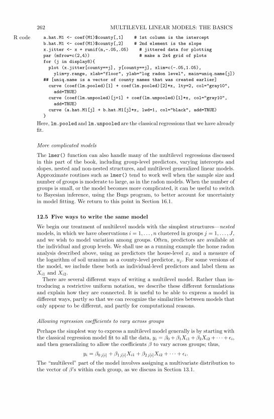
For a more elaborate example, we make Figure 12.4 using the following commands:


R code a.hat.M1 <- coef(M1)$county[,1] # 1st column is the interceptb.hat.M1 <- coef(M1)$county[,2] # 2nd element is the slopex.jitter <- x + runif(n,-.05,.05) # jittered data for plottingpar (mfrow=c(2,4)) # make a 2x4 grid of plotsfor (j in display8){plot (x.jitter[county==j], y[county==j], xlim=c(-.05,1.05),

ylim=y.range, xlab="floor", ylab="log radon level", main=uniq.name[j])## [uniq.name is a vector of county names that was created earlier]curve (coef(lm.pooled)[1] + coef(lm.pooled)[2]*x, lty=2, col="gray10",

add=TRUE)curve (coef(lm.unpooled)[j+1] + coef(lm.unpooled)[1]*x, col="gray10",

add=TRUE)curve (a.hat.M1[j] + b.hat.M1[j]*x, lwd=1, col="black", add=TRUE)

}

Here, lm.pooled and lm.unpooled are the classical regressions that we have alreadyfit.

More complicated models

The lmer() function can also handle many of the multilevel regressions discussedin this part of the book, including group-level predictors, varying intercepts andslopes, nested and non-nested structures, and multilevel generalized linear models.Approximate routines such as lmer() tend to work well when the sample size andnumber of groups is moderate to large, as in the radon models. When the number ofgroups is small, or the model becomes more complicated, it can be useful to switchto Bayesian inference, using the Bugs program, to better account for uncertaintyin model fitting. We return to this point in Section 16.1.

12.5 Five ways to write the same model

We begin our treatment of multilevel models with the simplest structures—nestedmodels, in which we have observations i = 1, . . . , n clustered in groups j = 1, . . . , J ,and we wish to model variation among groups. Often, predictors are available atthe individual and group levels. We shall use as a running example the home radonanalysis described above, using as predictors the house-level xi and a measure ofthe logarithm of soil uranium as a county-level predictor, uj. For some versions ofthe model, we include these both as individual-level predictors and label them asXi1 and Xi2.

There are several di!erent ways of writing a multilevel model. Rather than in-troducing a restrictive uniform notation, we describe these di!erent formulationsand explain how they are connected. It is useful to be able to express a model indi!erent ways, partly so that we can recognize the similarities between models thatonly appear to be di!erent, and partly for computational reasons.

Allowing regression coe!cients to vary across groups

Perhaps the simplest way to express a multilevel model generally is by starting withthe classical regression model fit to all the data, yi = !0 + !1Xi1 + !2Xi2 + · · ·+ "i,and then generalizing to allow the coe"cients ! to vary across groups; thus,

yi = !0 j[i] + !1 j[i]Xi1 + !2 j[i]Xi2 + · · · + "i.

The “multilevel” part of the model involves assigning a multivariate distribution tothe vector of !’s within each group, as we discuss in Section 13.1.

FIVE WAYS TO WRITE THE SAME MODEL 263

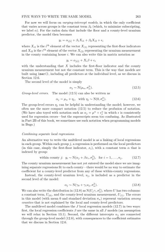
For now we will focus on varying-intercept models, in which the only coe!cientthat varies across groups is the constant term !0 (which, to minimize subscripting,we label "). For the radon data that include the floor and a county-level uraniumpredictor, the model then becomes

yi = "j[i] + !1Xi1 + !2Xi2 + #i

where Xi1 is the ith element of the vector X(1) representing the first-floor indicatorsand Xi2 is the ith element of the vector X(2) representing the uranium measurementin the county containing house i. We can also write this in matrix notation as

yi = "j[i] + Xi! + #i

with the understanding that X includes the first-floor indicator and the countyuranium measurement but not the constant term. This is the way that models arebuilt using lmer(), including all predictors at the individual level, as we discuss inSection 12.6.

The second level of the model is simply

"j ! N(µ!, $2!). (12.5)

Group-level errors. The model (12.5) can also be written as

"j = µ! + %j , with %j ! N(0, $2!). (12.6)

The group-level errors %j can be helpful in understanding the model; however, weoften use the more compact notation (12.5) to reduce the profusion of notation.(We have also toyed with notation such as "j = µ! + #!

j in which # is consistentlyused for regression errors—but the superscripts seem too confusing. As illustratedin Part 2B of this book, we sometimes use such notation when programming modelsin Bugs.)

Combining separate local regressions

An alternative way to write the multilevel model is as a linking of local regressionsin each group. Within each group j, a regression is performed on the local predictors(in this case, simply the first-floor indicator, xi), with a constant term " that isindexed by group:

within county j: yi ! N("j + !xi, $2y), for i = 1, . . . , nj . (12.7)

The county uranium measurement has not yet entered the model since we are imag-ining separate regressions fit to each county—there would be no way to estimate thecoe!cient for a county-level predictor from any of these within-county regressions.

Instead, the county-level uranium level, uj , is included as a predictor in thesecond level of the model:

"j ! N(&0 + &1uj , $2!). (12.8)

We can also write the distribution in (12.8) as N(Uj&, $2!), where U has two columns:

a constant term, U(0), and the county-level uranium measurement, U(1). The errorsin this model (with mean 0 and standard deviation $!) represent variation amongcounties that is not explained by the local and county-level predictors.

The multilevel model combines the J local regression models (12.7) in two ways:first, the local regression coe!cients ! are the same in all J models (an assumptionwe will relax in Section 13.1). Second, the di"erent intercepts "j are connectedthrough the group-level model (12.8), with consequences to the coe!cient estimatesthat we discuss in Section 12.6.


Group-level errors. We can write (12.8) as

!j = "0 + "1uj + #j , with #j ! N(0, $2!), (12.9)

explicitly showing the errors in the county-level regression.

Modeling the coe!cients of a large regression model

The identical model can be written as a single regression, in which the local andgroup-level predictors are combined into a single matrix X :

yi ! N(Xi%, $2y), (12.10)

where, for our example, X includes vectors corresponding to:• A constant term, X(0);

• The floor where the measurement was taken, X(1);

• The county-level uranium measure, X(2);

• J (not J"1) county indicators, X(3), . . . , X(J+2).At the upper level of the model, the J county indicators (which in this case are%3, . . . , %J+2) follow a normal distribution:

%j ! N(0, $2!), for j = 3, . . . , J + 2. (12.11)

In this case, we have centered the %j distribution at 0 rather than at an estimatedµ" because any such µ" would be statistically indistinguishable from the constantterm in the regression. We return to this point shortly.

The parameters in the model (12.10)–(12.11) can be identified exactly with thosein the separate local regressions above:• The local predictor x in model (12.7) is the same as X(1) (the floor) here.

• The local errors &i are the same in the two models.

• The matrix of group-level predictors U in (12.8) is just X(0) here (the constantterm) joined with X(2) (the uranium measure).

• The group-level errors #1, . . . , #J in (12.9) are identical to %3, . . . , %J+2 here.

• The standard-deviation parameters $y and $! keep the same meanings in thetwo models.

Moving the constant term around. The multilevel model can be written in yetanother equivalent way by moving the constant term:

yi = N(Xi%, $2y), for i = 1, . . . , n

%j ! N(µ!, $2!), for j = 3, . . . , J + 2. (12.12)

In this version, we have removed the constant term from X (so that it now has onlyJ +2 columns) and replaced it by the equivalent term µ! in the group-level model.The coe!cients %3, . . . , %J+2 for the group indicators are now centered around µ!

rather than 0, and are equivalent to !1, . . . , !J as defined earlier, for example, inmodel (12.9).

Regression with multiple error terms

Another option is to re-express model (12.10), treating the group-indicator coe!-cients as error terms rather than regression coe!cients, in what is often called a

GROUP-LEVEL PREDICTORS 265

“mixed e!ects” model popular in the social sciences:

yi ! N(Xi! + "j[i], #2y), for i = 1, . . . , n

"j ! N(0, #2!), (12.13)

where j[i] represents the county that contains house i, and X now contains onlythree columns:

• A constant term, X(0);

• The floor, X(1);

• The county-level uranium measure, X(2).

This is the same as model (12.10)–(12.11), simply renaming some of the !j ’s as"j ’s. All our tools for multilevel modeling will automatically work for models withmultiple error terms.

Large regression with correlated errors

Finally, we can express a multilevel model as a classical regression with correlatederrors:

yi = Xi! + $alli , $all ! N(0, "), (12.14)

where X is now the matrix with three predictors (the constant term, first-floorindicator, and county-level uranium measure) as in (12.13), but now the errors $alli

have an n " n covariance matrix ". The error $alli in (12.14) is equivalent to thesum of the two errors, "j[i] + $i, in (12.13). The term "j[i], which is the same for allunits i in group j, induces correlation in $all.

In multilevel models, " is parameterized in some way, and these parameters areestimated from the data. For the nested multilevel model we have been consideringhere, the variances and covariances of the n elements of $all can be derived in termsof the parameters #y and #!:

For any unit i: "ii = var($alli ) = #2y + #2

!

For any units i, k within the same group j: "ik = cov($alli , $allk ) = #2!

For any units i, k in di!erent groups: "ik = cov($alli , $allk ) = 0.

It can also be helpful to express " in terms of standard errors and correlations:

sd($i) =!

"ii ="

#2y + #2

!

corr($i, $k) ="ik#"ii"kk

=

#"2

!

"2y+"2

!if j[i] = j[k]

0 if j[i] $= j[k].

We generally prefer modeling the multilevel e!ects explicitly rather than buryingthem as correlations, but once again it is useful to see how the same model can bewritten in di!erent ways.

12.6 Group-level predictors

Adding a group-level predictor to improve inference for group coe!cients %j

We continue with the radon example from Sections 12.2–12.3 to illustrate how amultilevel model handles predictors at the group as well as the individual levels.


!"#$%&'$(")!* "'+,'- ,..#/'#/'-0 1.&0!"2

#!"3 2+*")-2 )"42*3 2+$!.&'2

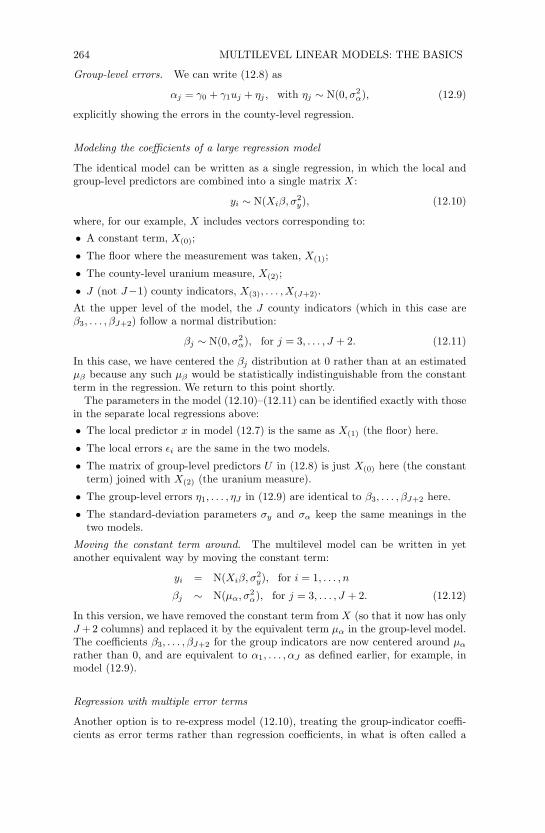
Figure 12.5 Multilevel (partial pooling) regression lines y = !j + "x fit to radon data,displayed for eight counties, including uranium as a county-level predictor. Light-coloredlines show the multilevel estimates, without uranium as a predictor, from Figure 12.4.

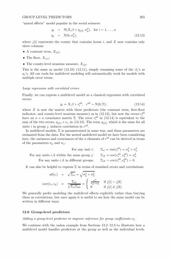
Figure 12.6 Estimated county coe!cients !j (±1 standard error) plotted versus county-level uranium measurement uj , along with the estimated multilevel regression line !j =#0 + #1uj . The county coe!cients roughly follow the line but not exactly; the deviation ofthe coe!cients from the line is captured in $!, the standard deviation of the errors in thecounty-level regression.

We use the formulation

yi ! N(!j[i] + "xi, #2y), for i = 1, . . . , n

!j ! N($0 + $1uj, #2!), for j = 1, . . . , J, (12.15)

where xi is the house-level first-floor indicator and uj is the county-level uraniummeasure.

R code u.full <- u[county]M2 <- lmer (y ~ x + u.full + (1 | county))display (M2)

This model includes floor, uranium, and intercepts that vary by county. The lmer()function only accepts predictors at the individual level, so we have converted uj toufull

i = uj[i] (with the variable county playing the role of the indexing j[i]), to pullout the uranium level of the county where house i is located.

The display of the lmer() fit shows coe!cients and standard errors, along withestimated residual variation at the county and individual (“residual”) level:


R outputlmer(formula = y ~ x + u.full + (1 | county))coef.est coef.se

(Intercept) 1.47 0.04x -0.67 0.07u.full 0.72 0.09Error terms:Groups Name Std.Dev.county (Intercept) 0.16Residual 0.76# of obs: 919, groups: county, 85deviance = 2122.9

As in our earlier example on page 261, we use coef() to pull out the estimatedcoe!cients,

R codecoef (M2)

yielding

R output$county(Intercept) x u.full

1 1.45 -0.67 0.722 1.48 -0.67 0.72. . .85 1.42 -0.67 0.72

Only the intercept varies, so the coe!cients for x and u.full are the same for all 85counties. (Actually, u.full is constant within counties so it cannot have a varyingcoe!cient here.) On page 280 we shall see a similar display for a model in whichthe coe!cient for x varies by county.

As before, we can also examine the estimated model averaging over the counties:

R codefixef (M2)

yielding

R output(Intercept) x u.full1.47 -0.67 0.72

and the county-level errors:

R coderanef (M2)

yielding

R output(Intercept)1 -0.022 0.01. . .85 -0.04

The results of fixef() and ranef() add up to the coe!cients in coef(): forcounty 1, 1.47 ! 0.02 = 1.45, for county 2, 1.47 + 0.01 = 1.48, . . . , and for county85, 1.47 ! 0.04 = 1.42 (up to rounding error).


Interpreting the coe!cients within counties

We can add the unmodeled coe!cients (the “fixed e"ects”) to the county-level errorsto get an intercept and slope for each county. We start with the model that averagesover all counties, yi = 1.47 ! 0.67xi + 0.72uj[i] (as obtained from display(M2) orfixef(M2).

Now consider a particular county, for example county 85. We can determine itsfitted regression line in two ways from the lmer() output, in each case using thelog uranium level in county 85, u85 = 0.36.

First, using the the last line of the display of coef(M2), the fitted model for county85 is yi = 1.42 ! 0.67xi + 0.72u85 = (1.42 + 0.72 · 0.36) ! 0.67xi = 1.68 ! 0.67xi,that is, 1.68 for a house with a basement and 1.01 for a house with no basement.Exponentiating gives estimated geometric mean predictions of 5.4 pCi/L and 2.7pCi/L for houses in county 85 with and without basements.

Alternatively, we can construct the fitted line for county 85 by starting with theresults from fixef(M2)—that is, yi = 1.47!0.67xi+0.72uj[i], setting uj[i] = u85 =0.36—and adding the group-level error from ranef(M2), which for county 85 is!0.04. The resulting model is yi = 1.47!0.67xi +0.72 ·0.36!0.04 = 1.68!0.67xi,the same as in the other calculation (up to rounding error in the last digit of theintercept).

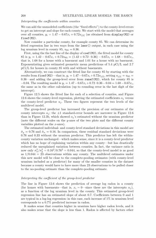
Figure 12.5 shows the fitted line for each of a selection of counties, and Figure12.6 shows the county-level regression, plotting the estimated coe!cients !j versusthe county-level predictor uj. These two figures represent the two levels of themultilevel model.

The group-level predictor has increased the precision of our estimates of thecounty intercepts !j : the ±1 standard-error bounds are narrower in Figure 12.6than in Figure 12.3b, which showed !j ’s estimated without the uranium predictor(note the di"erent scales on the y-axes of the two plots and the di"erent countyvariables plotted on the x-axes).

The estimated individual- and county-level standard deviations in this model are"y = 0.76 and "! = 0.16. In comparison, these residual standard deviations were0.76 and 0.33 without the uranium predictor. This predictor has left the within-county variation unchanged—which makes sense, since it is a county-level predictorwhich has no hope of explaining variation within any county—but has drasticallyreduced the unexplained variation between counties. In fact, the variance ratio isnow only "2

!/"2y = 0.162/0.762 = 0.044, so that the county-level model is as good

as 1/0.044 = 23 observations within any county. The multilevel estimates underthis new model will be close to the complete-pooling estimates (with county-leveluranium included as a predictor) for many of the smaller counties in the datasetbecause a county would have to have more than 23 observations to be pulled closerto the no-pooling estimate than the complete-pooling estimate.

Interpreting the coe!cient of the group-level predictor

The line in Figure 12.6 shows the prediction of average log radon in a county(for homes with basements—that is, xi = 0—since these are the intercepts !j),as a function of the log uranium level in the county. This estimated group-levelregression line has an estimated slope of about 0.7. Coe!cients between 0 and 1are typical in a log-log regression: in this case, each increase of 1% in uranium levelcorresponds to a 0.7% predicted increase in radon.

It makes sense that counties higher in uranium have higher radon levels, and italso makes sense that the slope is less than 1. Radon is a"ected by factors other


than soil uranium, and the “uranium” variable in the dataset is itself an imprecisemeasure of actual soil uranium in the county, and so we would expect a 1% increasein the uranium variable to match to something less than a 1% increase in radon.Compared to classical regression, the estimation of this coe!cient is trickier (sincethe !j ’s—the “data” for the county-level regression—are not themselves observed)but the principles of interpretation do not change.

A multilevel model can include county indicators along with a county-levelpredictor

Users of multilevel models are often confused by the idea of including county in-dicators along with a county-level predictor. Is this possible? With 85 counties inthe dataset, how can a regression fit 85 coe!cients for counties, plus a coe!cientfor county-level uranium? This would seem to induce perfect collinearity into theregression or, to put it more bluntly, to attempt to learn more than the data cantell us. Is it really possible to estimate 86 coe!cients from 85 data points?

The short answer is that we really have more than 85 data points. There arehundreds of houses with which to estimate the 85 county-level intercepts, and 85counties with which to estimate the coe!cient of county-level uranium. In a classicalregression, however, the 85 county indicators and the county-level predictor wouldindeed be collinear. This problem is avoided in a multilevel model because of thepartial pooling of the !j ’s toward the group-level linear model. This is illustrated inFigure 12.6, which shows the estimates of all these 86 parameters—the 85 separatepoints and the slope of the line. In this model that includes a group-level predictor,the estimated intercepts are pulled toward this group-level regression line (ratherthan toward a constant, as in Figure 12.3b). The county-level uranium predictoruj thus helps us estimate the county intercepts !j but without overwhelming theinformation in individual counties.

Partial pooling of group coe!cients !j in the presence of group-level predictors

Equation (12.4) on page 258 gives the formula for partial pooling in the simplemodel with no group-level predictors. Once we add a group-level regression, !j !N(Uj", #2

!), the parameters !j are shrunk toward their regression estimates !j =Uj". Equivalently, we can say that the group-level errors $j (in the model !j =Uj" + $j) are shrunk toward 0. As always, there is more pooling when the group-level standard deviation #! is small, and more smoothing for groups with fewerobservations. The multilevel estimate of !j is a weighted average of the no-poolingestimate for its group (yj " Xj%) and the regression prediction !j :

estimate of !j #nj

"2y

nj

"2y

+ 1"2

!

· (estimate from group j) +

+1

"2!

nj

"2y

+ 1"2

!

· (estimate from regression). (12.16)

Equivalently, the group-level errors $j are partially pooled toward zero:

estimate of $j #nj

"2y

nj

"2y

+ 1"2

!

(yj " Xj% " Uj") +1

"2!

nj

"2y

+ 1"2

!

· 0.


12.7 Model building and statistical significance

From classical to multilevel regression

When confronted with a multilevel data structure, such as the radon measurementsconsidered here or the examples in the previous chapter, we typically start by fittingsome simple classical regressions and then work our way up to a full multilevelmodel. The four natural starting points are:• Complete-pooling model: a single classical regression completely ignoring the

group information—that is, a single model fit to all the data, perhaps includinggroup-level predictors but with no coe!cients for group indicators.

• No-pooling model: a single classical regression that includes group indicators(but no group-level predictors) but with no model for the group coe!cients.

• Separate models: a separate classical regression in each group. This approach isnot always possible if there are groups with small sample sizes. (For example,in Figure 12.4 on page 257, Aitkin County has three measurements in homeswith basements and one in a home with no basement. If the sample from AitkinCounty had happened to contain only houses with basements, then it would beimpossible to estimate the slope ! from this county alone.)

• Two-step analysis: starting with either the no-pooling or separate models, thenfitting a classical group-level regression using, as “data,” the estimated coe!-cients for each group.

Each of these simpler models can be informative in its own right, and they also setus up for understanding the partial pooling in a multilevel model, as in Figure 12.4.

For large datasets, fitting a model separately in each group can be computa-tionally e!cient as well. One might imagine an iterative procedure that starts byfitting separate models, continues with the two-step analysis, and then returns tofitting separate models, but using the resulting group-level regression to guide theestimates of the varying coe!cients. Such a procedure, if formalized appropriately,is in fact the usual algorithm used to fit multilevel models, as we discuss in Chapter17.

When is multilevel modeling most e!ective?

Multilevel model is most important when it is close to complete pooling, at leastfor some of the groups (as for Lac Qui Parle County in Figure 12.4 on page 257).In this setting we can allow estimates to vary by group while still estimating themprecisely. As can be seen from formula (12.16), estimates are more pooled when thegroup-level standard deviation "! is small, that is, when the groups are similar toeach other. In contrast, when "! is large, so that groups vary greatly, multilevelmodeling is not much better than simple no-pooling estimation.

At this point, it might seem that we are contradicting ourselves. Earlier we mo-tivated multilevel modeling as a compromise between no pooling and completepooling, but now we are saying that multilevel modeling is e"ective when it is closeto complete pooling, and ine"ective when it is close to no pooling. If this is so, whynot just always use the complete-pooling estimate?

We answer this question in two ways. First, when the multilevel estimate is closeto complete pooling, it still allows variation between groups, which can be impor-tant, in fact can be one of the goals of the study. Second, as in the radon example,the multilevel estimate can be close to complete pooling for groups with small sam-

MODEL BUILDING AND STATISTICAL SIGNIFICANCE 271

ple size and close to no pooling for groups with large sample size, automaticallyperforming well for both sorts of group.

Using group-level predictors to make partial pooling more e!ective

In addition to being themselves of interest, group-level predictors play a specialrole in multilevel modeling by reducing the unexplained group-level variation andthus reducing the group-level standard deviation !!. This in turn increases theamount of pooling done by the multilevel estimate (see formula (12.16)), giving moreprecise estimates of the "j ’s, especially for groups for which the sample size nj issmall. Following the template of classical regression, multilevel modeling typicallyproceeds by adding predictors at the individual and group levels and reducingthe unexplained variance at each level. (However, as discussed in Section 21.7,adding a group-level predictor can actually increase the unexplained variance insome situations.)

Statistical significance

It is not appropriate to use statistical significance as a criterion for including par-ticular group indicators in a multilevel model. For example, consider the simplevarying-intercept radon model with no group-level predictor, in which the averageintercept µ! is estimated at 1.46, and the within-group intercepts "j are estimatedat 1.46! 0.27± 0.25 for county 1, 1.46! 0.53± 0.10 for county 2, 1.46+0.02± 0.28for county 3, and so forth (see page 261).

County 1 is thus approximately 1 standard error away from the average interceptof 1.46, county 2 is more than 4 standard errors away, . . . and county 85 is less than1 standard error away. Of these three counties, only county 2 would be considered“statistically significantly” di!erent from the average.

However, we should include all 85 counties in the model, and nothing is lost bydoing so. The purpose of the multilevel model is not to see whether the radon levelsin county 1 are statistically significantly di!erent from those in county 2, or fromthe Minnesota average. Rather, we seek the best possible estimate in each county,with appropriate accounting for uncertainty. Rather than make some significancethreshold, we allow all the intercepts to vary and recognize that we may not havemuch precision in many of the individual groups. We illustrate this point in anotherexample in Section 21.8.

The same principle holds for the models discussed in the following chapters, whichinclude varying slopes, non-nested levels, discrete data, and other complexities.Once we have included a source of variation, we do not use statistical significanceto pick and choose indicators to include or exclude from the model.

In practice, our biggest constraints—the main reasons we do not use extremelyelaborate models in which all coe"cients can vary with respect to all groupingfactors—are fitting and understanding complex models. The lmer() function workswell when it works, but it can break down for models with many grouping factors.Bugs is more general (see Part 2B of this book) but can be slow with large datasetsor complex models. In the meantime we need to start simple and build up gradually,a process during which we can also build understanding of the models being fit.


12.8 Predictions for new observations and new groups

Predictions for multilevel models can be more complicated than for classical re-gression because we can apply the model to existing groups or new groups. Aftera brief review of classical regression prediction, we explain in the context of theradon model.

Review of prediction for classical regression

In classical regression, prediction is simple: specify the predictor matrix X for a setof new observations5 and then compute the linear predictor X!, then simulate thepredictive data:

• For linear regression, simulate independent normal errors "i with mean 0 andstandard deviation #, and compute y = X! + "; see Section 7.2.

• For logistic regression, simulate the predictive binary data: Pr(yi) = logit!1(Xi!)for each new data point i; see Section 7.4.

• With binomial logistic regression, specify the number of tries ni for each newunit i, and simulate yi from the binomial distribution with parameters ni andlogit!1(Xi!); see Section 7.4.

• With Poisson regression, specify the exposures ui for the new units, and simulateyi ! Poisson(uieXi!) for each new i; see Section 7.4.

As discussed in Section 7.2, the estimation for a regression in R gives a set of nsims

simulation draws. Each of these is used to simulate the predictive data vector y,yielding a set of nsims simulated predictions. For example, in the election forecastingexample of Figure 7.5 on page 146:

R code model.1 <- lm (vote.88 ~ vote.86 + party.88 + inc.88)display (model.1)n.sims <- 1000sim.1 <- sim (model.1, n.sims)beta.sim <- sim.1$betasigma.sim <- sim.1$sigman.tilde <- length (vote.88)X.tilde <- cbind (rep(1,n.tilde), vote.88, party.90, inc.90)y.tilde <- array (NA, c(n.sims, n.tilde))for (s in 1:n.sims) {y.tilde[s,] <- rnorm (n.tilde, X.tilde%*%beta.sim[s,], sigma.sim[s])

}

This matrix of simulations can be used to get point predictions (for example,median(y.tilde[,3]) gives the median estimate for y3) or predictive intervals(for example, quantile(y.tilde[,3],c(.025,.975))) for individual data pointsor for more elaborate derived quantities, such as the predicted number of seatswon by the Democrats in 1990 (see the end of Section 7.3). For many applications,the predict() function in R is a good way to quickly get point predictions andintervals (see page 48); here we emphasize the more elaborate simulation approachwhich allows inferences for arbitrary quantities.

5 Predictions are more complicated for time-series models: even when parameters are fit by clas-sical regression, predictions must be made sequentially. See Sections 8.4 and 24.2 for examples.

PREDICTIONS FOR NEW OBSERVATIONS AND NEW GROUPS 273

Prediction for a new observation in an existing group

We can make two sorts of predictions for the radon example: predicting the radonlevel for a new house within one of the counties in the dataset, and for a new housein a new county. We shall work with model (12.15) on page 266, with floor as anindividual-level predictor and uranium as a group-level predictor

For example, suppose we wish to predict y, the log radon level for a house with nobasement (thus, with radon measured on the first floor, so that x = 1) in HennepinCounty (j = 26 of our Minnesota dataset). Conditional on the model parameters,the predicted value has a mean of !26 + " and a standard deviation of #y . That is,

y|$ ! N(!26 + "x, #2y),

where we are using $ to represent the entire vector of model parameters.Given estimates of !, ", and #y , we can create a predictive simulation for y using

R code such as

R codex.tilde <- 1sigma.y.hat <- sigma.hat(M2)$sigma$datacoef.hat <- as.matrix(coef(M2)$county)[26,]y.tilde <- rnorm (1, coef.hat %*% c(1, x.tilde, u[26]), sigma.y.hat)

More generally, we can create a vector of n.sims simulations to represent the pre-dictive uncertainty in y:

R coden.sims <- 1000coef.hat <- as.matrix(coef(M2)$county)[26,]y.tilde <- rnorm (1000, coef.hat %*% c(1, x.tilde, u[26]), sigma.y.hat)

Still more generally, we can add in the inferential uncertainty in the estimatedparameters, !, ", and #. For our purposes here, however, we shall ignore inferentialuncertainty and just treat the parameters !, ", #y , #! as if they were estimatedperfectly from the data.6 In that case, the computation gives us 1000 simulationdraws of y, which we can summarize in various ways. For example,

R codequantile (y.tilde, c(.25,.5,.75))

gives us a predictive median of 0.76 and a 50% predictive interval of [0.26, 1.27].Exponentiating gives us a prediction on the original (unlogged) scale of exp(0.76) =2.1, with a 50% interval of [1.3, 3.6].

For some applications we want the average, rather than the median, of the pre-dictive distribution. For example, the expected risk from radon exposure is propor-tional to the predictive average or mean, which we can compute directly from thesimulations:

R codeunlogged <- exp(y.tilde)mean (unlogged)

In this example, the predictive mean is 2.9, which is a bit higher than the medianof 2.1. This makes sense: on the unlogged scale, this predictive distribution is skewedto the right.

6 One reason we picked Hennepin County (j = 26) for this example is that, with a sample sizeof 105, its average radon level is accurately estimated from the available data.


Prediction for a new observation in a new group

Now suppose we want to predict the radon level for a house, once again with nobasement, but this time in a county not included in our analysis. We then mustgenerate a new county-level error term, !, which we sample from its N("0+"1uj, #2

!)distribution. We shall assume the new county has a uranium level equal to theaverage of the uranium levels in the observed counties:

R code u.tilde <- mean (u)

grab the estimated "0, "1, #! from the fitted model:

R code g.0.hat <- fixef(M2)["(Intercept)"]g.1.hat <- fixef(M2)["u.full"]sigma.a.hat <- sigma.hat(M2)$sigma$county

and simulate possible intercepts for the new county:

R code a.tilde <- rnorm (n.sims, g.0.hat + g.1.hat*u.tilde, sigma.a.hat)

We can then simulate possible values of the radon level for the new house in thiscounty:

R code y.tilde <- rnorm (n.sims, a.tilde + b.hat*x.tilde, sigma.y.hat)

Each simulation draw of y uses a di!erent simulation of !, thus propagating theuncertainty about the new county into the uncertainty about the new house in thiscounty.Comparison of within-group and between-group predictions. The resulting predic-tion will be more uncertain than for a house in a known county, since we have noinformation about !. Indeed, the predictive 50% interval of this new y is [0.28, 1.34],which is slightly wider than the predictive interval of [0.26, 1.27] for the new housein county 26. The interval is only slightly wider because the within-county variationin this particular example is much higher than the between-county variation.

More specifically, from the fitted model on page 266, the within-county (residual)standard deviation #y is estimated at 0.76, and the between-county standard devi-ation #! is estimated at 0.16. The log radon level for a new house in an already-measured county can then be measured to an accuracy of about ±0.76. The logradon level for a new house in a new county can be predicted to an accuracy ofabout ±

!0.762 + 0.162 = ±0.78. The ratio 0.78/0.76 is 1.03, so we would expect

the predictive interval for a new house in a new county to be about 3% widerthan for a new house in an already-measured county. The change in interval widthis small here because the unexplained between-county variance is so small in thisdataset.

For another example, the 50% interval for the log radon level of a house with nobasement in county 2 is [0.28, 1.30], which is centered in a di!erent place but alsois narrower than the predictive interval for a new county.

Nonlinear predictions

Section 7.3 illustrated the use of simulation for nonlinear predictions from classicalregression. We can perform similar calculations in multilevel models. For example,suppose we are interested in the average radon level among all the houses in Hen-nepin County (j = 26). We can perform this inference using poststratification, firstestimating the average radon level of the houses with and without basements in thecounty, then weighting these by the proportion of houses in the county that have

HOW MANY GROUPS AND OBSERVATIONS ARE NEEDED? 275

basements. We can look up this proportion from other data sources on homes, orwe can estimate it from the available sample data.

For our purposes here, we shall assume that 90% of all the houses in HennepinCounty have basements. The average radon level of all the houses in the county isthen 0.1 times the average for the houses in Hennepin County without basements,plus 0.9 times the average for those with basements. To simulate in R:

R codey.tilde.basement <- rnorm (n.sims, a.hat[26], sigma.y.hat)y.tilde.nobasement <- rnorm (n.sims, a.hat[26] + b.hat, sigma.y.hat)

We then compute the estimated mean for 1000 houses of each type in the county(first exponentiating since our model was on the log scale):

R codemean.radon.basement <- mean (exp (y.tilde.basement))mean.radon.nobasement <- mean (exp (y.tilde.nobasement))

and finally poststratify given the proportion of houses of each type in the county:

R codemean.radon <- .9*mean.radon.basement + .1*mean.radon.basement

In Section 16.6 we return to the topic of predictions, using simulations from Bugsto capture the uncertainty in parameter estimates and then propagating inferentialuncertainty into the predictions, rather than simply using point estimates a.hat,b.hat, and so forth.

12.9 How many groups and how many observations per group areneeded to fit a multilevel model?

Advice is sometimes given that multilevel models can only be used if the number ofgroups is higher than some threshold, or if there is some minimum number of obser-vations per groups. Such advice is misguided. Multilevel modeling includes classicalregression as a limiting case (complete pooling when group-level variances are zero,no pooling when group-level variances are large). When sample sizes are small, thekey concern with multilevel modeling is the estimation of variance parameters, butit should still work at least as well as classical regression.

How many groups?

When J , the number of groups, is small, it is di!cult to estimate the between-groupvariation and, as a result, multilevel modeling often adds little in such situations,beyond classical no-pooling models. The di!culty of estimating variance parametersis a technical issue to which we return in Section 19.6; to simplify, when !! cannotbe estimated well, it tends to be overestimated, and so the partially pooled estimatesare close to no pooling (this is what happens when !! has a high value in (12.16)on page 269).

At the same time, multilevel modeling should not do any worse than no-poolingregression and sometimes can be easier to interpret, for example because one caninclude indicators for all J groups rather than have to select one group as a baselinecategory.

One or two groups

With only one or two groups, however, multilevel modeling reduces to classicalregression (unless “prior information” is explicitly included in the model; see Section18.3). Here we usually express the model in classical form (for example, including


a single predictor for female, rather than a multilevel model for the two levels ofthe sex factor).

Even with only one or two groups in the data, however, multilevel models canbe useful for making predictions about new groups. See also Sections 21.2–22.5 forfurther connections between classical and multilevel models, and Section 22.6 forhierarchical models for improving estimates of variance parameters in settings withmany grouping factors but few levels per factor.

How many observations per group?

Even two observations per group is enough to fit a multilevel model. It is evenacceptable to have one observation in many of the groups. When groups have fewobservations, their !j ’s won’t be estimated precisely, but they can still provide par-tial information that allows estimation of the coe!cients and variance parametersof the individual- and group-level regressions.

Larger datasets and more complex models

As more data arise, it makes sense to add parameters to a model. For example,consider a simple medical study, then separate estimates for men and women, otherdemographic breakdowns, di"erent regions of the country, states, smaller geographicareas, interactions between demographic and geographic categories, and so forth.As more data become available it makes sense to estimate more. These complexitiesare latent everywhere, but in small datasets it is not possible to learn so much, andit is not necessarily worth the e"ort to fit a complex model when the resultinguncertainties will be so large.

12.10 Bibliographic note

Multilevel models have been used for decades in agriculture (Henderson, 1950,1984, Henderson et al., 1959, Robinson, 1991) and educational statistics (Novicket al., 1972, 1973, Bock, 1989), where it is natural to model animals in groupsand students in classrooms. More recently, multilevel models have become popu-lar in many social sciences and have been reviewed in books by Longford (1993),Goldstein (1995), Kreft and De Leeuw (1998), Snijders and Bosker (1999), Verbekeand Molenberghs (2000), Leyland and Goldstein (2001), Hox (2002), and Rauden-bush and Bryk (2002). We do not attempt to trace here the many applications ofmultilevel models in various scientific fields.

It might also be useful to read up on Bayesian inference to understand the the-oretical background behind multilevel models.7 Box and Tiao (1973) is a classicreference that focuses on linear models. It predates modern computational meth-ods but might be useful for understanding the fundamentals. Gelman et al. (2003)and Carlin and Louis (2000) cover applied Bayesian inference including the basics ofmultilevel modeling, with detailed discussions of computational algorithms. Berger

7 As we discuss in Section 18.3, multilevel inferences can be formulated non-Bayesianly; however,understanding the Bayesian derivations should help with the other approaches too. All mul-tilevel models are Bayesian in the sense of assigning probability distributions to the varyingregression coe!cients. The distinction between Bayesian and non-Bayesian multilevel mod-els arises only for the question of modeling the other parameters—the nonvarying coe!cientsand the variance parameters—and this is typically a less important issue, especially when thenumber of groups is large.

EXERCISES 277

(1985) and Bernardo and Smith (1994) cover Bayesian inference from two di!erenttheoretical perspectives.

The R function lmer() is described by Bates (2005a, b) and was developed fromthe linear and nonlinear mixed e!ects software described in Pinheiro and Bates(2000).

Multilevel modeling used to be controversial in statistics; see, for example, thediscussions of the papers by Lindley and Smith (1972) and Rubin (1980) for somesense of the controversy.

The Minnesota radon data were analyzed by Price, Nero, and Gelman (1996);see also Price and Gelman (2004) for more on home radon modeling.

Statistical researchers have studied partial pooling in many ways; see James andStein (1960), Efron and Morris (1979), DuMouchel and Harris (1983), Morris (1983),and Stigler (1983). Louis (1984), Shen and Louis (1998), Louis and Shen (1999), andGelman and Price (1999) discuss some di"culties in the interpretation of partiallypooled estimates. Zaslavsky (1993) discusses adjustments for undercount in theU.S. Census from a partial-pooling perspective. Normand, Glickman, and Gatsonis(1997) discuss the use of multilevel models for evaluating health-care providers.

12.11 Exercises

1. Using data of your own that are appropriate for a multilevel model, write themodel in the five ways discussed in Section 12.5.

2. Continuing with the analysis of the CD4 data from Exercise 11.4:

(a) Write a model predicting CD4 percentage as a function of time with varyingintercepts across children. Fit using lmer() and interpret the coe"cient fortime.

(b) Extend the model in (a) to include child-level predictors (that is, group-levelpredictors) for treatment and age at baseline. Fit using lmer() and interpretthe coe"cients on time, treatment, and age at baseline.

(c) Investigate the change in partial pooling from (a) to (b) both graphically andnumerically.

(d) Compare results in (b) to those obtained in part (c).

3. Predictions for new observations and new groups:

(a) Use the model fit from Exercise 12.2(b) to generate simulation of predictedCD4 percentages for each child in the dataset at a hypothetical next timepoint.

(b) Use the same model fit to generate simulations of CD4 percentages at each ofthe time periods for a new child who was 4 years old at baseline.

4. Posterior predictive checking: continuing the previous exercise, use the fittedmodel from Exercise 12.2(b) to simulate a new dataset of CD4 percentages (withthe same sample size and ages of the original dataset) for the final time point ofthe study, and record the average CD4 percentage in this sample. Repeat thisprocess 1000 times and compare the simulated distribution to the observed CD4percentage at the final time point for the actual data.

5. Using the radon data, include county sample size as a group-level predictor andwrite the varying-intercept model. Fit this model using lmer().

6. Return to the beauty and teaching evaluations introduced in Exercise 3.5 and4.8.


(a) Write a varying-intercept model for these data with no group-level predictors.Fit this model using lmer() and interpret the results.

(b) Write a varying-intercept model that you would like to fit including threegroup-level predictors. Fit this model using lmer() and interpret the results.

(c) How does the variation in average ratings across instructors compare to thevariation in ratings across evaluators for the same instructor?

7. This exercise will use the data you found for Exercise 4.7. This time, rather thanrepeating the same analysis across each year, or country (or whatever group thedata varies across), fit a multilevel model using lmer() instead. Compare theresults to those obtained in your earlier analysis.

8. Simulate data (outcome, individual-level predictor, group indicator, and group-level predictor) that would be appropriate for a multilevel model. See how partialpooling changes as you vary the sample size in each group and the number ofgroups.

9. Number of observations and number of groups:

(a) Take a simple random sample of one-fifth of the radon data. (You can cre-ate this subset using the sample() function in R.) Fit the varying-interceptmodel with floor as an individual-level predictor and log uranium as a county-level predictor, and compare your inferences to what was obtained by fittingthe model to the entire dataset. (Compare inferences for the individual- andgroup-level standard deviations, the slopes for floor and log uranium, the av-erage intercept, and the county-level intercepts.)

(b) Repeat step (a) a few times, with a di!erent random sample each time, andsummarize how the estimates vary.

(c) Repeat step (a), but this time taking a cluster sample: a random sample ofone-fifth of the counties, but then all the houses within each sampled county.

Documents

Multilevel linear models: the basicsvulstats.ucsd.edu/pdf/Gelman.ch-12.basic-multilevel-models.pdfMultilevel linear models: the basics Multilevel modeling can be thought of in two