Multilevel k-way Partitioning Scheme for Irregular Graphs

JOURNAL OF PARALLEL AND DISTRIBUTED COMPUTING48, 96–129 (1998)ARTICLE NO. PC971404

Multilevel k-way Partitioning Schemefor Irregular Graphs1

George Karypis2 and Vipin Kumar3

Department of Computer Science/Army HPC Research Center, Unviersity of Minnesota,

Minneapolis, Minnesota 55455

In this paper, we present and study a class of graph partitioning algorithmsthat reduces the size of the graph by collapsing vertices and edges, we finda k-way partitioning of the smaller graph, and then we uncoarsen and refineit to construct ak-way partitioning for the original graph. These algorithmscompute ak-way partitioning of a graphG = (V, E) in O(|E|) time, whichis faster by a factor ofO(log k) than previously proposed multilevel recursivebisection algorithms. A key contribution of our work is in finding a high-qualityand computationally inexpensive refinement algorithm that can improve upon aninitial k-way partitioning. We also study the effectiveness of the overall schemefor a variety of coarsening schemes. We present experimental results on a largenumber of graphs arising in various domains including finite element methods,linear programming, VLSI, and transportation. Our experiments show that thisnew scheme produces partitions that are of comparable or better quality thanthose produced by the multilevel bisection algorithm and requires substantiallysmaller time. Graphs containing up to 450,000 vertices and 3,300,000 edges canbe partitioned in 256 domains in less than 40 s on a workstation such as SGI’sChallenge. Compared with the widely used multilevel spectral bisection algorithm,our new algorithm is usually two orders of magnitude faster and produces partitionswith substantially smaller edge-cut.© 1998 Academic Press

Key Words: graph partitioning; multilevel partitioning methods; Kernighan–Lin heuristic; spectral partitioning methods; parallel sparse matrix algorithms.

1This work was supported by NSF CCR-9423082, by the Army Research Office Contract DA/DAAH04-95-1-0538, by the IBM Partnership Award, and by the Army High Performance Computing Research Center underthe auspices of the Department of the Army, Army Research Laboratory Cooperative Agreement NumberDAAH04-95-2-0003/Contract DAAH04-95-C-0008, the content of which does not necessarily reflect theposition or the policy of the government, and no official endorsement should be inferred. Access to computingfacilities was provided by AHPCRC, Minnesota Supercomputer Institute, Cray Research Inc., and the PittsburghSupercomputing Center. Related papers are available via WWW at URL: http://www.cs.umn.edu/∼karypis.

2E-mail: [email protected]: [email protected].

96

0743-7315/98 $25.00Copyright © 1998 by Academic PressAll rights of reproduction in any form reserved.

MULTILEVEL k-WAY PARTITIONING SCHEME 97

1. INTRODUCTION

The graph partitioning problem is to partition the vertices of a graph inp roughlyequal partitions such that the number of edges connecting vertices in different partitionsis minimized. This problem finds applications in many areas including parallel scientificcomputing, task scheduling, and VLSI design. Some examples are domain decompositionfor minimum communication mapping in the parallel execution of sparse linear systemsolvers, mapping of spatially related data items in large geographical information systemson disk to minimize disk I/O requests, and mapping of task graphs to parallel processors.The graph partitioning problem is NP-complete. However, many algorithms have beendeveloped that find reasonably good partitionings [2, 3, 5, 7–9, 12, 13, 16, 18–24].

The k-way partitioning problem is most frequently solved by recursive bisection. Thatis, we first obtain a 2-way partitioning ofV, and then we recursively obtain a 2-waypartitioning of each resulting partition. After logk phases, graphG is partitioned intok partitions. Thus, the problem of performing ak-way partitioning is reduced to thatof performing a sequence of bisections. Recently [2, 12, 16], a multilevel recursivebisection (MLRB) algorithm has emerged as a highly effective method for computing ak-way partitioning of a graph. The basic structure of a multilevel bisection algorithm isvery simple. The graphG is first coarsened down to a few hundred vertices, a bisection ofthis much smaller graph is computed, and then this partitioning is projected back to theoriginal graph (finer graph) by periodically refining the partitioning. Since the finer graphhas more degrees of freedom, such refinements decrease the edge-cut. The experimentspresented in [16] show that compared to the state-of-the-art implementation of the well-known spectral bisection [1], MLRB produces partitionings that are significantly betterand is an order of magnitude faster. The complexity of the MLRB for producing ak-waypartitioning of a graphG = (V, E), is O(|E| log k) [16].

The multilevel paradigm can also be used to construct ak-way partitioning of thegraph directly as illustrated in Fig. 1. The graph is coarsened successively as before.But the coarsest graph is now directly partitioned intok parts, and thisk-partitioningis refined successively as the graph is uncoarsened back into the original graph. Thereare a number of advantages of computing thek-way partitioning directly (rather thancomputing it successively via recursive bisection). First, the entire graph now needs tobe coarsened only once, reducing the complexity of this phase toO(|E|) down fromO(|E| log k). Second, it is well known that recursive bisection can do arbitrarily worsethan k-way partitioning [27]. Thus, a method that obtains ak-way partitioning directlycan potentially produce much better partitionings. Note that the direct computation ofa goodk-way partitioning is harder than the computation of a good bisection (althoughboth problems are NP-hard) in general. This is precisely whyk-way partitioning is mostcommonly computed via recursive bisection. But in the context of multilevel schemes,we only need a roughk-way partitioning of the coarsest graph, as this can be potentiallyrefined successively as the graph is uncoarsened. For example, a simple method forcomputing this initial partitioning in the multilevel context is simply to coarsen thegraph down tok vertices. However, in the refinement phase, we need to refine ak-waypartitioning, which is considerably more complicated than refining a bisection. In fact, adirect generalization of the KL refinement algorithm tok-way partitioning used in [10]is substantially more expensive than performing a KL refinement of a bisection [17].

98 KARYPIS AND KUMAR

FIG. 1. The various phases of the multilevelk-way partitioning algorithm. During the coarsening phase,the size of the graph is successively decreased; during the initial partitioning phase, ak-way partitioning ofthe smaller graph is computed (a 6-way partitioning in this example); and during the uncoarsening phase, thepartitioning is successively refined as it is projected to the larger graphs.

Even for 8-way refinement, the run time is quite high for these schemes [11]. Computingk-way refinement fork > 8 is prohibitively expensive.

In this paper, we present ak-way partitioning algorithm. The run time of thisk-way multilevel algorithm (MLkP) is linear to the number of edges, i.e.,O(|E|). Akey contribution of our work is a simple and yet powerful scheme for refining ak-way partitioning in the multilevel context. This scheme is substantially faster than thedirect generalization [11] of the KL bisection refinement algorithm, but it is equallyeffective in the multilevel context. Furthermore, this newk-way refinement algorithm isinherently parallel [15] (unlike the original KL refinement algorithm which is known tobe inherently sequential in nature [6]), making it possible to develop high-quality parallelgraph partitioning algorithms.

We test our scheme on a large number of graphs arising in various domains includingfinite element methods, linear programming, VLSI, and transportation. Our experimentsshow that this new scheme produces partitionings that are of comparable or better qualitythan those produced by the state-of-the-art implementation of the MLRB algorithm [16],and it requires substantially smaller time. Graphs containing up to 450,000 vertices and3,300,000 edges, can be partitioned in 256 partitions in less than 40 s on a workstationsuch as SGI’s Challenge. For many of these graphs, the process of graph partitioning takeseven less time than the time to read the graph from the disk into memory. Compared withthe widely used multilevel spectral bisection algorithm [12, 22, 23], our new algorithmis usually two orders of magnitude faster and produces partitionings with substantiallysmaller edge-cut. The run time of ourk-way partitioning algorithm is comparable tothe run time of a small number (2–4) runs of geometric recursive bisection algorithms[9, 18–20, 24]. Note that geometric algorithms are applicable only if coordinates of the


vertices are available and require tens of runs to produce cuts that are of quality similarto those produced by spectral bisection.

The remainder of the paper is organized as follows. Section 2 defines the graph parti-tioning problem and presents the basic concepts of multilevelk-way graph partitioning.Some of the material presented in this section on coarsening strategies is similar to thatfor multilevel recursive bisection [12, 16], but it is included here to make this paper selfcontained. Section 3 presents an experimental evaluation of the various parameters ofthe multilevel graph partitioning algorithm and compares its performance with that of amultilevel recursive bisection algorithm.

2. GRAPH PARTITIONING

The k-way graph partitioning problem is defined as follows: Given a graphG = (V,E) with |V| = n, partitionV into k subsets,V1, V2, . . . , Vk such thatVi ∩ Vj = ∅ for i ≠ j,|Vi| = n/k, and

⋃i Vi = V, and the number of edges ofE whose incident vertices belong

to different subsets is minimized. Ak-way partitioning ofV is commonly represented bya partitioning vectorP of lengthn, such that for every vertexv ∈ V, P[v] is an integerbetween 1 andk, indicating the partition to which vertexv belongs. Given a partitioningP, the number of edges whose incident vertices belong to different partitions is calledthe edge-cutof the partitioning.

The basic structure of a multilevelk-way partitioning algorithm is very simple. Thegraph G = (V, E) is first coarsened down to a small number of vertices, ak-waypartitioning of this much smaller graph is computed, and then this partitioning is projectedback toward the original graph (finer graph) by successively refining the partitioning ateach intermediate level. This three-stage process of coarsening, initial partitioning, andrefinement is graphically illustrated in Fig. 1.

Next we describe each of these phases in more detail.

2.1. Coarsening Phase

During the coarsening phase, a sequence of smaller graphsGi = (Vi, Ei), is constructedfrom the original graphG0 = (V0, E0) such that |Vi| < |Vi−1|. In most coarsening schemes,a set of vertices ofGi is combined to form a single vertex of the next level coarser graphGi+1. Let Vv

i be the set of vertices ofGi combined to form vertexv of Gi+1. In orderfor a partitioning of a coarser graph to be good with respect to the original graph, theweight of vertexv is set equal to the sum of the weights of the vertices inVv

i . Also, inorder to preserve the connectivity information in the coarser graph, the edges ofv arethe union of the edges of the vertices inVv

i . In the case where more than one vertex ofVv

i contain edges to the same vertexu, the weight of the edge ofv is equal to the sumof the weights of these edges. This coarsening method ensures the following properties[12]: (i) the edge-cut of the partitioning in a coarser graph is equal to the edge-cut ofthe same partition in the finer graph and (ii) a balanced partitioning of the coarser graphleads to a balanced partitioning of the finer graph.

This edge collapsing idea can be formally defined in terms of matchings [2, 12]. Amatchingof a graph is a set of edges, no two of which are incident on the same vertex.Thus, the next level coarser graphGi+1 is constructed fromGi by finding a matching ofGi and collapsing the vertices being matched into multinodes. The unmatched vertices are


simply copied over toGi+1. Since the goal of collapsing vertices is to decrease the size ofthe graphGi, the matching should be maximal. A matching is calledmaximal matchingif it is not possible to add any other edge to it without making two edges become incidenton the same vertex. Note that depending on how matchings are computed, the size ofthe maximal matching may be different.

The coarsening phase ends when the coarsest graphGm has a small number of verticesor if the reduction in the size of successively coarser graphs becomes too small. In ourexperiments, for ak-way partition, we stop the coarsening process when the number ofvertices becomes less thanck, wherec = 15 in our experiments. The choice of this valueof c was to allow the initial partitioning algorithm to createk partitions of roughly thesame size. We also end the coarsening phase if the reduction in the size of successivegraphs is less than a factor of 0.8.

In the remaining sections we describe three ways that we used to select maximalmatchings for coarsening. Two of these matchings, RM [2, 12] and HEM [16], havebeen previously investigated in the context of MLRB.

Random Matching (RM).A maximal matching can be generated efficiently using arandomized algorithm. In our experiments we used a randomized algorithm similar tothat described in [2, 12, 16]. The random maximal matching algorithm works as follows.The vertices are visited in random order. If a vertexu has not been matched yet, thenwe randomly select one of its unmatched adjacent vertices. If such a vertexv exists, weinclude the edge (u, v) in the matching and mark verticesu andv as being matched. Ifthere is no unmatched adjacent vertexv, then vertexu remains unmatched in the randommatching. The complexity of the above algorithm isO(|E|).

Heavy Edge Matching (HEM).Random matching is a simple and efficient method tocompute a maximal matching and minimizes the number of coarsening levels in a greedyfashion. However, our overall goal is to find a partitioning that minimizes the edge-cut.Consider a graphGi = (Vi, Ei), a matchingMi that is used to coarsenGi, and its coarsergraphGi+1 = (Vi+1, Ei+1) induced byMi. If A is a set of edges, defineW(A) to be thesum of the weights of the edges inA. It can be shown that

W(Ei+1) = W(Ei )−W(Mi ). (1)

Thus, the total edge-weight of the coarser graph is reduced by the weight of the match-ing. Hence, by selecting a maximal matchingMi whose edges have a large weight, wecan decrease the edge-weight of the coarser graph by a greater amount. As the analy-sis in [13] shows, since the coarser graph has smaller edge-weight, it also has a smalleredge-cut.

Finding a maximal matching that contains edges with large weight is the idea behind theheavy-edge matchingoriginally introduced in [16]. A heavy-edge matching is computedusing a randomized algorithm similar to that for computing a random matching describedearlier. The vertices are again visited in random order. However, instead of randomlymatching a vertexu with one of its adjacent unmatched vertices, we matchu with thevertexv such that the weight of the edge (u, v) is maximum over all valid incident edges(heavier edge). Note that this algorithm does not guarantee that the matching obtainedhas maximum weight (over all possible matchings), but our experiments have shown that


it works very well in practice. The complexity of computing a heavy-edge matching isO(|E|), which is asymptotically similar to that for computing the random matching.

Modified Heavy Edge Matching (HEM*).The analysis of the multilevel bisectionalgorithm in [13] shows that a good edge-cut of a coarser graph is closer to that of agood edge-cut of the original graph if the average degree of the coarser graph is small. Themodified heavy edge matching(HEM*) is a modification of HEM that tries to decreasethe average degree of coarser graphs.

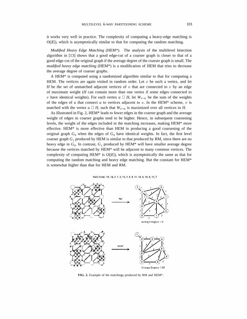
A HEM* is computed using a randomized algorithm similar to that for computing aHEM. The vertices are again visited in random order. Letv be such a vertex, and letH be the set of unmatched adjacent vertices ofv that are connected tov by an edgeof maximum weight (H can contain more than one vertex if some edges connected tov have identical weights). For each vertexu ∈ H, let Wv–u be the sum of the weightsof the edges ofu that connectu to vertices adjacent tov. In the HEM* scheme,v ismatched with the vertexu ∈ H, such thatWv–u is maximized over all vertices inH.

As illustrated in Fig. 2, HEM* leads to fewer edges in the coarser graph and the averageweight of edges in coarser graphs tend to be higher. Hence, in subsequent coarseninglevels, the weight of the edges included in the matching increases, making HEM* moreeffective. HEM* is more effective than HEM in producing a good coarsening of theoriginal graphG0 when the edges ofG0 have identical weights. In fact, the first levelcoarser graphG1 produced by HEM is similar to that produced by RM, since there are noheavy edge inG0. In contrast,G1 produced by HEM* will have smaller average degreebecause the vertices matched by HEM* will be adjacent to many common vertices. Thecomplexity of computing HEM* isO(|E|), which is asymptotically the same as that forcomputing the random matching and heavy edge matching. But the constant for HEM*is somewhat higher than that for HEM and RM.

FIG. 2. Example of the matchings produced by RM and HEM*.


2.2. Initial Partitioning Phase

The second phase of a multilevelk-way partitioning algorithm is to compute ak-waypartitioning Pm of the coarse graphGm = (Vm, Em) such that each partition containsroughly |V0|/k vertex weight of the original graph. Since during coarsening, the weightsof the vertices and edges of the coarser graph were set to reflect the weights of thevertices and edges of the finer graph,Gm contains sufficient information to intelligentlyenforce the balanced partitioning and the minimum edge-cut requirements.

One way to produce the initialk-way partitioning is to keep coarsening the graphuntil it has only k vertices left. These coarsek vertices can serve as the initialk-waypartitioning of the original graph. There are two problems with this approach. First, formany graphs, the reduction in the size of the graph in each coarsening step becomesvery small after some coarsening steps, making it very expensive to continue with thecoarsening process. Second, even if we are able to coarsen the graph down to onlykvertices, the weights of these vertices are likely to be quite different, making the initialpartitioning highly unbalanced.

In our algorithm, thek-way partitioning of Gm is computed using our multilevelbisection algorithm [16]. Our experience has shown that our multilevel recursive bisectionalgorithm produces good initial partitionings and requires a relatively small amount oftime as long as the size of the original graph is sufficiently larger thank.

2.3. Uncoarsening Phase

During the uncoarsening phase, the partitioningPm of the coarser graphGm is projectedback to the original graph, by going through the graphsGm−1, Gm−2, . . . , G1. Since eachvertexv of Gi+1 contains a distinct subset of verticesVv

i of Gi, Pi is obtained fromPi+1

by simply assigning the set of verticesVvi to the partitioningPi+1[v]; i.e., Pi[u] = Pi+1[v],

∀u ∈ Vvi .

Note that, even if the partitioning ofGi is at a local minima,4 the projected partitioningof Gi−1 may not be at a local minima. SinceGi−1 is finer, it has more degrees of freedomthat can be used to further improve the partitioning and thus decrease the edge-cut. Hence,it may still be possible to improve the projected partitioning ofGi−1 by local refinementheuristics.

A class of local refinement algorithms that tends to produce very good results arethose based on the Kernighan–Lin (KL) partitioning algorithm [17] and their variants [4,12]. The KL algorithm incrementally swaps vertices among partitions of a bisection toreduce the edge-cut of the partitioning until the partitioning reaches a local minima. Onecommonly used variation of the KL algorithm for bisection refinement is from Fiduccia–Mattheyses [4]. In particular, for each vertexv, this variation of the KL algorithmcomputes thegain which is the reduction in the edge-cut achieved by movingv tothe other partition. These vertices are inserted into two priority queues, one for eachpartition, according to their gains. Initially, all vertices areunlocked; i.e., they are freeto move to the other partition. The algorithm iteratively selects an unlocked vertexv

with the largest gain from one of the two priority queues and moves it to the otherpartition. When a vertexv is moved, it islockedand the gain of the vertices adjacent to

4A partitioning is at a local minima, if movement of any vertex from one part to the other does not improvethe edge-cut.


v are updated. After each vertex movement, the algorithm also records the size of thecut achieved at this point. Note that the algorithm does not allow locked vertices to bemoved since this may result in thrashing (i.e., repeated movement of the same vertex). Asingle pass of the algorithm ends when there are no more unlocked vertices (i.e., all thevertices have been moved). Then, the recorded cut-sizes are checked, the point where theminimum cut was achieved is selected, and all vertices that were moved after that pointare moved back to their original partition. Now, this becomes the initial partitioning forthe next pass of the algorithm. In the case of multilevel recursive bisection algorithms[2, 12, 16], KL refinement becomes very powerful, as the initial partitioning available ateach successive uncoarsening level is already a good partition.

However, refining ak-way partitioning is significantly more complicated becausevertices can move from a partition to many other partitions; thus, increasing theoptimization space combinatorially. An extension of the KL refinement algorithm inthe case ofk-way refinement is described in [10]. This algorithm usesk(k − 1) priorityqueues, one for each type of move. In each step of the algorithm, the moves with thehighest gain are found from each of thesek(k − 1) queues, and the move with the highestgain that preserves or improves the balance is performed. After the move, all of thek(k− 1) priority queues are updated. The complexity ofk-way refinement is significantlyhigher than that of 2-way refinement, and for a graph withm edges, this complexityis O(k * m). This approach is only practical for small values ofk. Due to this highcomplexity, the multilevel recursive octasection algorithm described in [10], requires thesame amount of time as multilevel recursive bisection, even though recursive octasectionspends much less time for coarsening.

We have developed simplek-way refinement algorithms that are simplified versionsof the k-way Kernighan–Lin refinement algorithm, and their complexity is independentof the number of partitions being refined. As the results in Section 3 show, despite thesimplicity of our refinement algorithms, they produce high quality partitionings in a smallamount of time. First, we describe some key concepts and definitions that are used inthe description of our twok-way partitioning refinement algorithms.

Consider a graphGi = (Vi, Ei) and its partitioning vectorPi. For each vertexv ∈ Vi

we define theneighborhood N(v) of v to be the union of the partitions that the verticesadjacent tov (i.e., Adj(v)) belong to; that is,N(v) = ∪u∈Ad j(v)Pi[u]. Note that ifv is aninterior vertex of a partition, thenN(v) = ∅. On the other hand, the cardinality ofN(v)can be as high asAdj(v) for the case in which each vertex adjacent tov belongs to adifferent partition. During refinement,v can move to any of the partitions inN(v). Foreach vertexv we compute the gains of movingv to one of its neighbor partitions. Inparticular, for everyb ∈ N(v) we computeED[v] b as the sum of the weights of the edges(v, u) such thatPi[u] = b. Also, we computeID[v] as the sum of the weights of theedges (v, u) such thatPi[u] = Pi[v]. The quantityED[v] b is called theexternal degreeofv to partitionb, while the quantityID[v] is called theinternal degreeof v. Given thesedefinitions, the gain of moving vertexv to partition b ∈ N(v) is g[v] b − ID[v]. Thesedefinitions are illustrated in Fig. 3. For example, for vertex 5,N[5] = {0, 2}, ID[5] = 2,ED[5] 0 = 2, andED[5] 2 = 3.

However, in addition to decreasing the edge-cut, moving a vertex from one partition toanother must not create partitions whose size is unbalanced. In particular, our partitioningrefinement algorithms move a vertex only if it satisfies the followingBalancing Condition.


FIG. 3. Illustration of neighboring partitions and internal and external vertex degrees.

Let Wi be a vector ofk elements, such thatWi[a] is the weight of partitiona of graphGi, and letWmin = 0.9|V0|/k and Wmax = C|V0|/k. A vertex v, whose weight isw(v) canbe moved from partitiona to partitionb only if

Wi [b] +w(v) ≤Wmax, (2)

and

Wi [a] −w(v) ≥Wmin (3)

The first condition ensures that movement of a node into a partition does not make itsweight higher thanWmax. Note that by adjusting the value ofC, we can vary the degreeof imbalance among partitions. IfC = 1, then the refinement algorithm tries to make eachpartition of equal weight. In our experiments we found that lettingC be greater than 1.0,tends to improve the quality of the partitionings. However, in order to minimize the loadimbalance, we usedC = 1.03; that puts an upper bound of 3% on load imbalance. Notethat the second condition is not critical for load balance, but it ensures that there is nopartition with too few vertices.

Greedy Refinement (GR).The lookahead in KL algorithm serves a very importantpurpose. It allows movement of an entire cluster of vertices across a partition boundary.Note that it is quite possible that as the cluster is moved across the partition boundary, theedge-cut increases, but after the entire cluster of vertices moves across the partition, thenthe overall edge-cut comes down. In the context of multilevel schemes, this lookaheadbecomes less important. The reason is that these clusters of vertices are coarsened into asingle vertex at successive coarsening phases. Hence, movement of a vertex at a coarselevel actually corresponds to the movement of a group of vertices in the original graph.

If the lookahead part of KL is eliminated (i.e., if vertices are moved only if they leadto positive gain), then it becomes less useful to maintain a priority queue. In particular,vertices whose move results in a large positive gain will be moved anyway even if theyare not moved earlier in the priority order. Hence, a variation of KL that simply visitsthe boundary vertices in a random order and moves them if they result in a positive gain


is likely to work well in the multilevel context. Ourgreedy refinementalgorithm is basedon this observation. It consists of a number of iterations. In each iteration, all the verticesare checked to see if they can be moved so that either the edge-cut of the partitioningcan be decreased (while preserving balance), or the balance is improved.

In particular, GR works as follows. Consider a graphGi = (Vi, Ei), and its partitioningvectorPi. The vertices are checked in a random order. Letv be such a vertex, letPi[v]= a be the partition thatv belongs to. Ifv is a node internal to partitiona thenN(v) = ∅,andv is not moved. Ifv is at the boundary of the partition, thenN(v) is nonempty. LetN ′(v) be the subset ofN(v) that contains all partitionsb such that movement of vertexv to partitionb does not violate the Balancing Condition. Now vertexv is moved to oneof the adjacent partitionsb, if either one of the following conditions is satisfied:

1. ED[v] b > ID[v] and ED[v] b is maximum among allb ∈ N ′(v).2. ED[v] b = ID(v) andWi[a] − Wi[b] > w(v).

That is, the GR algorithm movesv to a partition that leads to the largest reduction inthe edge-cut without violating the balance condition. If no reduction in the edge-cut ispossible, by movingv, thenv is moved to the partition (if any) that leads to no increasein the edge-cut but improves the balance. After moving vertexv, the algorithm updatesthe internal and external degrees of the vertices adjacent tov to reflect the change inthe partition.

The GR algorithm converges after a small number of iterations. In our experiments, wefound that for most graphs, and with the HEM (or HEM*) matching scheme in particular,GR converged within four to eight iterations.

Global Kernighan–Lin Refinement (GKLR).As discussed in the previous section,the GR algorithm lacks any capabilities of climbing out of local minima. Our secondrefinement heuristic calledglobal Kernighan–Lin, is somewhat more powerful and iscloser to the original KL algorithm in spirit. It adds some limited hill-climbing capabilitiesto the GR algorithm and also uses a priority queue to determine the sequence ofvertex moves.

The GKLR algorithm uses a global priority queue that stores the vertices accordingto their gains. Initially, all the vertices are scanned, and those whose sum of externaldegrees5 is greater or equal to their internal degrees are inserted into the priority queue.In particular, letv be such a vertex, letN(v) be the neighborhood ofv, and b ∈ N(v)such thatED[v] b is maximum over the external degrees of partitions inN(v). We insertv into the priority queue with a gain equal toED[v] b − ID[v].

The algorithm then proceeds and selects the vertex from the priority queue with thehighest gain. Having selected such a vertexv, the algorithm selects a partb ∈ N(v) tomovev such thatED[v] b is maximized while satisfying the balance condition (Eqs. (2)and (3)). Note that these swaps may lead to an increase in the edge-cut, since vertices aremoved even if they have a negative gain value. The GKLR algorithm continues movingvertices until it has performedx vertex moves that have not decreased the overall edge-

5We used this heuristic to select the vertices that are inserted in the priority queue as a compromise betweeninserting all the boundary vertices and inserting only the vertices that lead to a reduction in the edge-cut whenmoved to one of their neighboring partitions. If all the boundary vertices were inserted, then the cost wouldhave been higher. On the other hand, if only the edge-cut reducing vertices were inserted, the hill-climbingcapabilities of the algorithm would have been reduced.


cut. In that case, the lastx moves are undone. Once a vertex is moved, it is not consideredfor movement in the same iteration. This is repeated for a small number of iterations oruntil convergence.

Note that in each step, the vertices selected for movement by the GKLR algorithm andby the generalized KL of [11] may be quite different. GKLR selects a vertexv that hasa move (among all possible moves to neighboring partitionsN(v)) with the highest gaing[v] max. However, depending on the weight of the partitions, this move may never takeplace, and insteadv can be moved to a partitiona ∈ N(v) that leads to a smaller gaing[a]v. However, there may be another vertexu on the priority queue that has a movewith the highest gaing[u] max that may be permissible. Now ifg[v]v < g[u] max < g[v] max,the generalization of the KL algorithm will select to move vertexu before consideringvertexv. Thus, in each step, GKLR does not necessarily select the vertex with the largestrealizable gain. Furthermore, since the single priority queue contains only vertices whosesum of the external degrees in greater or equal to the internal degree, GKLR has lesspowerful hill-climbing capabilities than the generalized KL [11] that uses multiple priorityqueues and considers all the vertices.

3. EXPERIMENTAL RESULTS

We evaluated the performance of the multilevel graph partitioning algorithm on awide range of graphs arising in different application domains. The characteristics ofthese graphs are described in Table 1. These graphs are classified into six groups. Thefirst group contains graphs that correspond to finite element meshes, the second groupcontains graphs that correspond to coefficient matrices (i.e., assembled matrices) withmultiple degrees of freedom and linear basis functions, the third group corresponds toassembled matrices with nonlinear basis functions, the fourth group corresponds to graphsthat represent highway networks, the fifth group corresponds to graphs arising in linearprogramming applications, and the sixth group corresponds to graphs that represent VLSIcircuits. For each of the first two groups, we have a large number of graphs, but for thelast four groups, we have only a few graphs per group. So observed trends for the firsttwo groups are more reliable than those for the last four groups.

All the experiments were performed on an SGI Challenge with 1.2 GBytes of memoryand a 200 MHz MIPS R4400 processor. All times reported are in seconds. Since the natureof the multilevel algorithm discussed is randomized, we performed all experiments withfixed seed.

3.1. Matching Schemes

We implemented the three matching schemes described in Section 2.1. These schemesare (a) random matching (RM), (b) heavy edge matching (HEM), and (c) modified heavyedge matching (HEM*). For all the experiments, we used the GR refinement policy duringthe uncoarsening phase. The results for 32-way and 256-way partitioning are shown inFigs. 4 and 5 for all the graphs in Table 1.

In Fig. 4 we see that both HEM and HEM* consistently produce partitionings whoseedge-cut is better than that of the partitionings produced by RM. For some groups ofgraphs, HEM and HEM* produce partitionings whose edge-cut is better than that of RMby up to 35%. The reason for the poor performance of RM becomes clear in Table 2 that


TABLE 1

Various Graphs Used in Evaluating the Multilevel Graph Partitioning

and Sparse Matrix Ordering Algorithm

Matrix nameNumber

of vertices Number of edges Description

144 144649 1074393 3D Finite element mes (Parafoil)

598A 110971 741934 3D Finite element mesh (Submarine I)

AUTO 448695 3314611 3D Finite element mesh (GM Saturn)

BRACK2 62631 366559 3D Finite element mesh (Bracket)

COPTER2 55476 352238 3D Finite element mesh (Helicopter blade)

FLAP 51537 479620 3D Finite element mesh

M14B 214765 3358036 3D Finite element mesh (Submarine II)

ROTOR 99617 662431 3D Finite element mesh

TORSO 201142 1479989 3D Finite element mesh (Human torso)

WAVE 156317 1059331 3D Finite element mesh

BCSSTK31 35588 572914 3D Stiffness matrix

BCSSTK32 44609 985046 3D Stiffness matrix

CANT 54195 1960797 3D Stiffness matrix

CYLINDER93 45594 1786726 3D Stiffness matrix

INPRO1 46949 1117809 3D Stiffness matrix

SHELL93 181200 2313765 3D Stiffness matrix

SHYY161 76480 152002 CFD/Navier-Stokes

TROLL 213453 5885829 3D Stiffness matrix

VENKAT25 62424 827684 2D Coefficient matrix

BBMAT 38744 993481 2D Stiffness matrix

MAP1 267241 334931 Highway network

MAP2 78489 98995 Highway network

FINAN512 74752 261120 Linear programming

KEN-11 14694 33880 Linear programming

S38584.1 22143 35608 Sequential circuit

contains the size of the edge-cut of the initialk-way partitioning. For all graphs, the sizeof the initial edge-cut on the coarsest graph is significantly worse for RM compared withHEM and HEM*. Note that the difference in the size of the initial edge-cut on the coarsestgraph is much greater for the three schemes than those shown in Fig. 4. For example, forthe first two groups of graphs, the overall quality of RM, HEM, and HEM* is similar, butthe edge-cut of thek-way partitioning in the coarsest graph obtained by HEM and HEM*


FIG

.4.

Qua

lity

ofth

epa

rtiti

onin

gsof

HE

Man

dH

EM

*re

lativ

eto

RM

mat

chin

g.F

orea

chgr

aph,

the

ratio

ofth

eed

ge-c

utof

the

HE

Man

dH

EM

*m

atch

ing

sche

mes

toth

at

ofth

eR

Mm

atch

ing

sche

me

ispl

otte

dfo

r32

-an

d25

6-w

aypa

rtiti

onin

gs.

Bar

sun

der

the

base

line

indi

cate

that

the

corr

espo

ndin

gm

atch

ing

sche

me

perf

orm

sbe

tter

than

RM

.


FIG

.5.

Run

time

ofpa

rtiti

onin

gus

ing

HE

Man

dH

EM

*re

lativ

eto

RM

mat

chin

g.F

orea

chgr

aph,

the

ratio

ofth

etim

ere

quire

dby

the

HE

Man

dH

EM

*m

atch

ing

sche

mes

toth

atof

the

RM

mat

chin

gsc

hem

eis

plot

ted

for

32-

and

256-

way

part

ition

ings

.B

ars

unde

rth

eba

selin

ein

dica

teth

atth

eco

rres

pond

ing

mat

chin

gsc

hem

eis

fast

er

than

RM

.


are 30 to 65% smaller than those obtained by RM (as shown in Table 2). (As a result, forRM, k-way refinement takes more time compared with HEM and HEM*.) As discussed in[13], the effectiveness of a coarsening scheme depends on how successful it is in removinga significant amount of edge-weight from the successive coarser graphs. According tothis criterion, HEM and HEM* are strictly better coarsening schemes than RM becausethey remove more edge-weight from the graph.

Comparing HEM against HEM*, we see that for most graphs, their performance iscomparable. The only notable exception isBBMATfor which HEM* does up to 10%better than HEM.BBMATis the type of graph in which applying RM at the finest graph(G0) significantly increases the average degree of the first level coarser graph (G1). Notethat HEM and RM compute the same first level coarse graphG1, since the weights of alledges inG0 is the same. Hence, forBBMATthe average degree ofG1 obtained by HEMis much higher than that obtained using HEM*. For other types of graphs, particularlythose that correspond to finite element meshes, RM increases the average degree onlyslightly in going fromG0 to G1, which in turn allows HEM to perform good coarsening.As a result, forBBMAT, the initial partitioning found by HEM is much worse than thatfound by HEM*. This can be seen in Table 2. Note that the initial edge-cuts for HEMand HEM* are similar for all problems exceptBBMAT.

In Fig. 5 we see that for 32-way partition, HEM is up to 20% faster than RM, whileHEM* is up to 41% slower than RM. HEM is faster than RM because it requiresmuch less refinement, and the coarsening step of HEM is only slightly slower thanthe coarsening step in RM. HEM* is slower than RM because coarsening using HEM*is much slower than coarsening using RM. For a 256-way partition, HEM is again fasterthan RM (quite consistently), but now for 7 graphs HEM* is faster than RM. This isbecause RM requires substantially more refinement time and because the coarsest graphGm produced by RM has many more edges than that produced by HEM*, increasing theinitial partitioning time.

TABLE 2

Quality of Initial Partitionings for the RM,

HEM, and HEM* Matching Schemes

64EC 256EC

Graph RM HEM HEM* RM HEM HEM*

144 200855 142464 136949 292079 229401 223615

AUTO 525526 343154 334210 815578 575975 560929

FLAP 58034 42810 39394 119368 95452 92358

BCSSTK32 221234 155286 143176 342679 287300 265350

INPRO1 244035 159632 149373 405038 319496 301075

BBMAT 324794 154878 89305 584891 350850 196325

MAP2 1064 911 839 2382 2205 2173

KEN-11 16273 15677 15578 18697 18067 17813

Note. 64EC and 256EC are the edge-cuts of 64- and 256-way partitionings.


As the experiments show, for most of the graphs, HEM is an excellent matching schemethat produces good partitionings, and requires the smallest overall run time. However,for a certain class of graphs, HEM* does better than HEM.

3.2. Refinement Policies

As described in Section 2.3, there are different ways that a partitioning can be refinedduring the uncoarsening phase. We evaluated the performance of two refinement policies,both in terms of the quality of the partitionings they produce and also how much timethey require. The refinement policies that we evaluate are greedy refinement (GR) andglobal Kernighan–Lin refinement (GKLR).

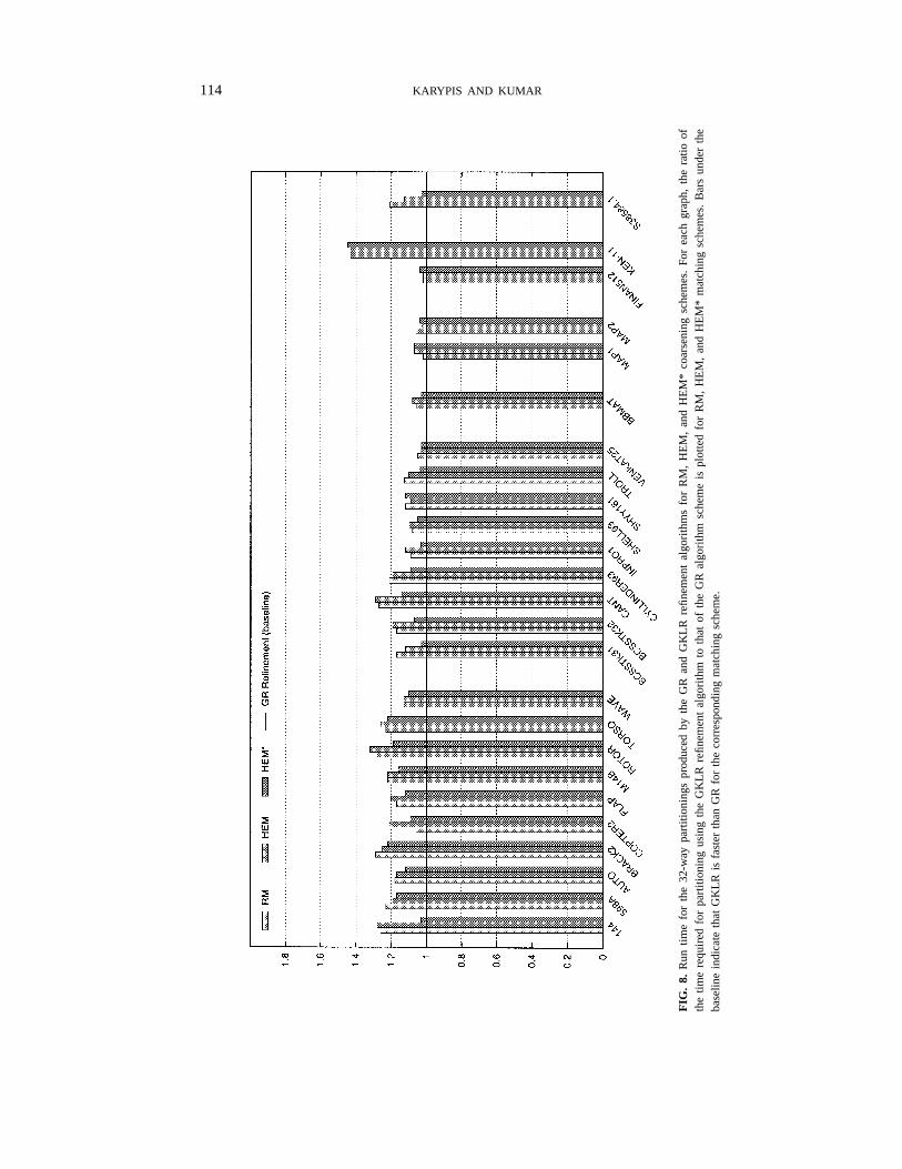
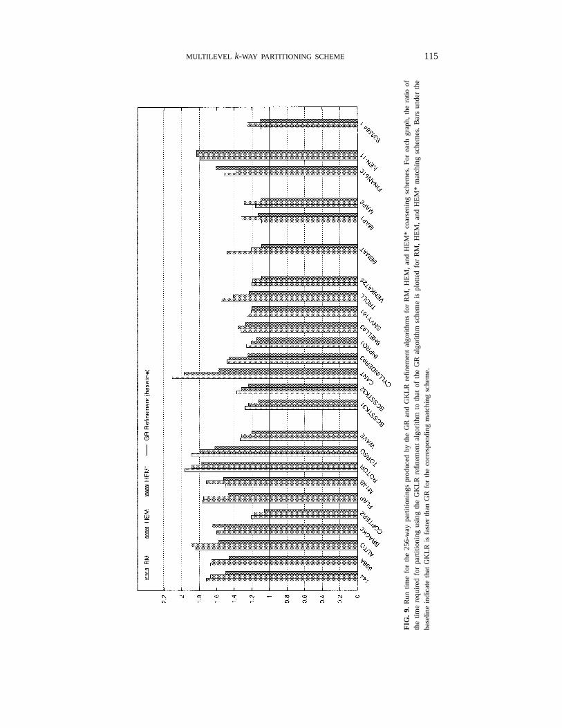
The results of these refinement policies for computing a 32- and 256-way partition forthe graphs in Table 1 are shown in Figs. 6–9. Figures 6 and 7 show the edge-cut of thepartitionings produced by GKLR relative to those produced by GR for the three differentcoarsening schemes, while Figs. 8 and 9 show the amount of time required by GKLRrelative to GR for computing these partitionings.

A number of observations can be made from Figs. 6 and 7. GKLR is significantly betterthan GR only forBBMAT. For other problems, the difference is minor. If RM coarsening isused, then GKLR does better than GR more consistently. If HEM or HEM* coarseningis used, then GKLR performs quite similar to GR for all problems. Even forBBMAT,the gap between the performance of GKLR and GR is narrower for HEM and HEM*compared with RM. If we combine the 32- and 256-way partitionings as a set of 150different runs, GKLR produces better partitionings for 31 out of these 150 runs. Outof these 31 runs, 14 were obtained using RM, 7 using HEM, and 10 using HEM*.Another interesting observation is that for most graphs the difference in the quality ofthe partitionings produced by GR and GKLR is very small. The difference in the qualityis less than 2% for 139 out of the 150 different runs. The only notable exceptions areKEN-11 for which GR does up to 7% better than GKLR andBBMATfor which GKLRdoes up to 21% better than GR. From these experimental results, it is clear that a simplerefinement scheme such as GR is quite adequate, particularly if the initial partitioningfor the coarsest graph is quite good. The additional power of GKLR is useful onlywhen it is used in conjunction with the RM matching scheme which leads to poor initialpartitionings.

From Figs. 8 and 9 we see that the amount of time required for a 32- and 256-waypartitioning using GKLR is significantly higher than the time required using GR. GKLRrequires more time for each of the 150 different runs. In some cases, GKLR requiresmore than twice the time required by GR. Comparing the different matching schemes,we see that the relative increase in the run time is higher for RM than for HEM andHEM*. This is not surprising since RM requires more refinement and also RM benefitsthe most from GKLR.

In summary, GR and GKLR tend to produce partitionings that have similar edge-cuts,but with GKLR requiring significantly more time than GR.

3.3. Comparison with Other Partitioning Schemes

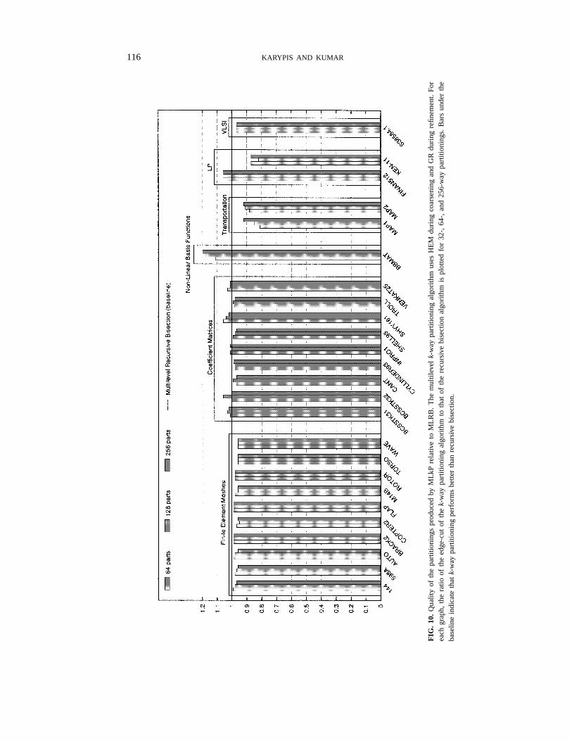
Figure 10 shows the relative quality of our multilevelk-way partitioning algorithm(MLkP) compared to the multilevel recursive bisection algorithm (MLRB) described in[16] (implemented in METIS [14]). METIS is a set of programs for partitioning unstructured


FIG

.6.

Qua

lity

ofG

KLR

refin

emen

tsc

hem

efo

r32

-way

part

ition

ing

for

RM

,H

EM

,an

dH

EM

*co

arse

ning

sche

mes

rela

tive

toG

Rre

finem

ent

sche

me.

For

each

grap

h,th

era

tioof

the

edge

-cut

ofth

eG

KLR

refin

emen

tal

gorit

hmto

that

ofth

eG

Ral

gorit

hmsc

hem

eis

plot

ted

for

RM

,H

EM

,an

dH

EM

*m

atch

ing

sche

mes

.B

ars

unde

rth

eba

selin

ein

dica

teth

atG

KLR

perf

orm

sbe

tter

than

GR

for

the

corr

espo

ndin

gm

atch

ing

sche

me.


FIG

.7.Q

ualit

yof

GK

LRre

finem

ent

sche

me

for

256-

way

part

ition

ing

for

RM

,H

EM

,an

dH

EM

*co

arse

ning

sche

mes

rela

tive

toG

Rre

finem

ent

sche

me.

For

each

grap

h,th

era

tioof

the

edge

-cut

ofth

eG

KLR

refin

emen

tal

gorit

hmto

that

ofth

eG

Ral

gorit

hmsc

hem

eis

plot

ted

for

RM

,H

EM

,an

dH

EM

*m

atch

ing

sche

mes

.B

ars

unde

rth

eba

selin

ein

dica

teth

atG

KLR

perf

orm

sbe

tter

than

GR

for

the

corr

espo

ndin

gm

atch

ing

sche

me.


FIG

.8.

Run

time

for

the

32-w

aypa

rtiti

onin

gspr

oduc

edby

the

GR

and

GK

LRre

finem

ent

algo

rithm

sfo

rR

M,

HE

M,

and

HE

M*

coar

seni

ngsc

hem

es.

For

each

grap

h,th

era

tio

ofth

etim

ere

quire

dfo

rpa

rtiti

onin

gus

ing

the

GK

LRre

finem

ent

algo

rithm

toth

atof

the

GR

algo

rithm

sche

me

ispl

otte

dfo

rR

M,

HE

M,

and

HE

M*

mat

chin

gsc

hem

es.

Bar

sun

der

the

base

line

indi

cate

that

GK

LRis

fast

erth

anG

Rfo

rth

eco

rres

pond

ing

mat

chin

gsc

hem

e.


FIG

.9.

Run

time

for

the

256-

way

part

ition

ings

prod

uced

byth

eG

Ran

dG

KLR

refin

emen

tal

gorit

hms

for

RM

,H

EM

,an

dH

EM

*co

arse

ning

sche

mes

.F

orea

chgr

aph,

the

ratio

ofth

etim

ere

quire

dfo

rpa

rtiti

onin

gus

ing

the

GK

LRre

finem

ent

algo

rithm

toth

atof

the

GR

algo

rithm

sche

me

ispl

otte

dfo

rR

M,

HE

M,

and

HE

M*

mat

chin

gsc

hem

es.

Bar

sun

der

the

base

line

indi

cate

that

GK

LRis

fast

erth

anG

Rfo

rth

eco

rres

pond

ing

mat

chin

gsc

hem

e.


FIG

.10

.Qua

lity

ofth

epa

rtiti

onin

gspr

oduc

edby

MLk

Pre

lativ

eto

MLR

B.

The

mul

tilev

elk-w

aypa

rtiti

onin

gal

gorit

hmus

esH

EM

durin

gco

arse

ning

and

GR

durin

gre

finem

ent.

For

each

grap

h,th

era

tioof

the

edge

-cut

ofth

ek-

way

part

ition

ing

algo

rithm

toth

atof

the

recu

rsiv

ebi

sect

ion

algo

rithm

ispl

otte

dfo

r32

-,64

-,an

d25

6-w

aypa

rtiti

onin

gs.

Bar

sun

der

the

base

line

indi

cate

thatk

-way

part

ition

ing

perf

orm

sbe

tter

than

recu

rsiv

ebi

sect

ion.


graphs and for ordering sparse matrices that implements various algorithms described in[16]. For each graph, we plot the ratio of the edge-cut of the MLkP algorithm to theedge-cut of the MLRB algorithm (the actual edge-cuts are shown in Table 3). Ratiosthat are less than one indicate that MLkP produces better partitionings than MLRB. For

TABLE 3

The Edge-Cuts Produced by the Multilevel Recursive Bisection, Multilevel

Recursive Bisection, and Multilevelk-way Partitioning

Multilevelspectral bisection

Multilevelrecursive bisection

Multilevelk-way partition

Matrix 64EC 128EC 256EC 64EC 128EC 256EC 64EC 128EC 256EC

144 96538 132761 184200 88806 120611 161563 87750 118112 156145

598A 68107 95220 128619 64443 89298 119699 63262 86909 114846

AUTO 208729 291638 390056 194436 269638 362858 193092 263228 349137

BRACK2 34464 49917 69243 29983 42625 60608 29742 42170 59847

COPTER2 47862 64601 84934 43721 58809 77155 42411 56100 73946

FLAP 35540 54407 80392 30741 49806 74628 30461 49203 73641

M14B 124749 172780 232949 111104 156417 214203 109013 150331 206129

ROTOR 63251 88048 120989 53228 75010 103895 52069 73841 101732

TORSO 413501 473397 522717 117997 160788 218155 112797 155087 209895

WAVE 106858 142060 187192 97978 129785 171101 94251 124377 164187

BCSSTK31 86244 123450 176074 65249 97819 140818 66039 100713 143749

BCSSTK32 130984 185977 259902 106440 152081 222789 106661 160651 223545

CANT 459412 598870 798866 442398 574853 778928 428754 567478 756061

CYLINDER93 290194 431551 594859 289639 416190 590065 284012 409445 582015

INPRO1 125285 185838 264049 116748 171974 250207 118176 172592 251628

SHELL93 178266 238098 318535 124836 185323 269539 123437 181203 261296

SHYY161 6641 9151 11969 4365 6317 9092 4607 6591 9251

TROLL 529158 706605 947564 453812 638074 864287 445215 630918 846822

VENKAT25 50184 77810 116211 47514 73735 110312 49137 74470 111249

BBMAT 179282 250535 348124 55753 92750 132387 62018 109495 158990

MAP1 3546 6314 8933 1388 2221 3389 1122 1892 3108

MAP2 1759 2454 3708 828 1328 2157 726 1213 1984

FINAN512 15360 27575 53387 11388 22136 40201 11853 23365 42589

KEN-11 20931 23308 25159 14257 16515 18101 12360 13563 15836

S38584.1 5381 7595 9609 2428 3996 5906 2362 3869 5715

Note. 64EC, 128EC, and 256EC are the edge-cuts of 64-, 128-, and 256-way partitionings, respectively.


FIG

.11

.Run

time

ofM

LkP

rela

tive

toM

LRB

for

256-

way

part

ition

ing.

The

mul

tilev

elk-w

aypa

rtiti

onin

gal

gorit

hmus

esH

EM

durin

gco

arse

ning

and

GR

durin

gre

finem

ent.

For

each

grap

h,th

era

tioof

the

run

time

ofre

curs

ive

bise

ctio

nal

gorit

hmto

that

ofth

ek-

way

part

ition

ing

algo

rithm

ispl

otte

dfo

r25

6-w

aypa

rtiti

onin

gs.

Bar

sab

ove

the

base

line

indi

cate

that

k-w

aypa

rtiti

onin

gis

fast

erth

anre

curs

ive

bise

ctio

n.


this comparison and for the rest of the comparisons in this section, the MLkP algorithmuses HEM during coarsening and GR during refinement.

From this figure, we see that for almost all problems, MLkP and MLRB producepartitionings of similar quality. In particular, for the two highway networks (MAP1

and MAP2), MLkP produces up to 19% smaller edge-cuts than MLRB. For the graphsthat correspond to finite element meshes (144, 598A, AUTO, BRACK2, COPTER2,

M14B, ROTOR, TORSO,and WAVE), MLkP does slightly (up to 5%) and consistentlybetter than MLRB. For the graphs that correspond to coefficient matrices of finiteelement applications with multiple degrees of freedom (BCSSTK31, BCSSTK32, CANT,

CYLINDER93, FLAP, INPRO1, SHELL93, SHYY161, TROLL, and VENKAT25), MLkPand MLRB perform quite similarly (within 6% of each other). The only problem for whichMLkP performs significantly worse than MLRB isBBMAT, for which MLkP performsup to 20% worse than MLRB. As discussed in Section 2.1, these graphs correspond toassembled matrices with nonlinear basis functions, and the HEM coarsening scheme doesnot lead to good coarsenings. However, for this graph, both HEM* coarsening and GKLRrefinement perform substantially better than HEM and GR, respectively. In particular, ifwe use HEM* for coarsening and GKLR for refinement, then the edge-cut for 128-waypartitioning produced by MLkP is better by 2% than that of MLRB. In summary, for alarge class of graphs, MLkP produces partitionings that are equally good or even betterthan those produced by the MLRB algorithm. Furthermore, the combination of HEM andGR seems quite adequate for most problems. However, for some problems HEM* andGKLR may be better choices for coarsening and refinement, respectively.

TABLE 4

The Time Required to Find a 256–Way Partitioning by the Multilevel Spectral Bisection,

Multilevel Recursive Bisection, and Multilevel k-way Partition (All Times Are in Seconds)

Matrix

Multilevelspectralbisection

Multilevelrecursivebisection

Multilevelk-way

partition Matrix

Multilevelspectral

bisection

Multilevelrecursivebisection

Multilevelk-way

partition

144 607.27 48.14 13.40 CYLINDER93 671.33 39.10 13.07

598A 420.12 35.05 9.92 INPRO1 341.88 24.60 7.88

AUTO 2214.24 179.15 39.67 SHELL93 1111.96 71.59 17.40

BRACK2 218.36 16.52 5.65 SHYY161 129.99 10.13 3.42

COPTER2 185.39 16.11 5.71 TROLL 3063.28 132.08 29.08

FLAP 279.67 16.50 5.21 VENKAT25 254.52 20.81 5.54

M14B 970.58 74.04 18.30 BBMAT 474.23 22.51 10.37

ROTOR 550.35 29.46 8.71 MAP1 850.16 44.80 8.12

TORSO 1053.37 63.93 17.13 MAP2 195.09 11.76 3.07

WAVE 658.13 44.55 12.94 FINAN512 311.01 17.98 6.49

BCSSTK31 309.06 15.21 5.53 KEN-11 121.94 4.09 3.13

BCSSTK32 474.64 22.50 7.39 S38584.1 178.11 4.72 2.55

CANT 978.48 47.70 17.44


FIG

.12

.Q

ualit

yof

MLk

Pre

lativ

eto

mul

tilev

elsp

ectr

albi

sect

ion.

For

each

grap

h,th

era

tioof

the

edge

-cut

ofth

ek-

way

part

ition

ing

algo

rithm

toth

atof

the

recu

rsiv

ebi

sect

ion

algo

rithm

ispl

otte

dfo

r32

-,64

-,12

8-,

and

256-

way

part

ition

ings

.B

ars

unde

rth

eba

selin

ein

dica

teth

atk-

way

part

ition

ing

perf

orm

sbe

tter

than

mul

tilev

elsp

ectr

albi

sect

ion.


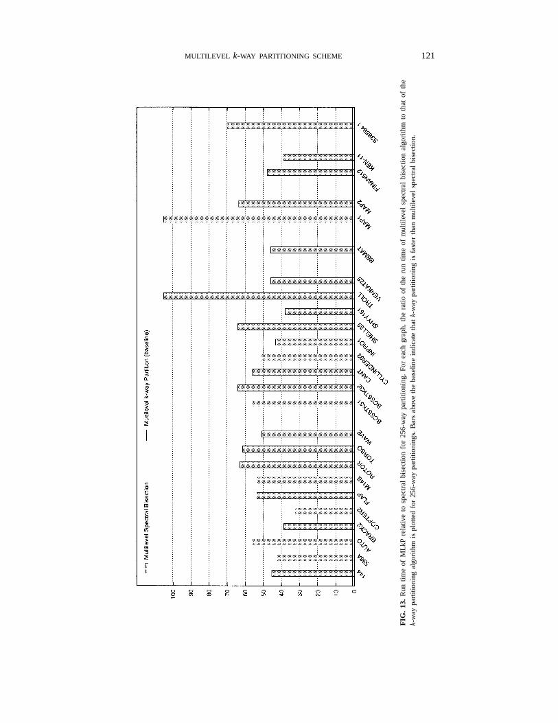
FIG

.13

.R

untim

eof

MLk

Pre

lativ

eto

spec

tral

bise

ctio

nfo

r25

6-w

aypa

rtiti

onin

g.F

orea

chgr

aph,

the

ratio

ofth

eru

ntim

eof

mul

tilev

elsp

ectr

albi

sect

ion

algo

rithm

toth

atof

the

k-w

aypa

rtiti

onin

gal

gorit

hmis

plot

ted

for

256-

way

part

ition

ings

.B

ars

abov

eth

eba

selin

ein

dica

teth

atk-

way

part

ition

ing

isfa

ster

than

mul

tilev

elsp

ectr

albi

sect

ion.



FIG

.14

.Q

ualit

yof

the

part

ition

ings

prod

uced

byM

LkP

rela

tive

toC

haco

’sm

ultil

evel

recu

rsiv

eoc

tase

ctio

nal

gorit

hm.

The

MLk

Pal

gorit

hmus

esH

EM

durin

gco

arse

ning

and

GR

durin

gre

finem

ent.

For

each

grap

h,th

era

tioof

the

edge

-cut

ofth

eM

LkP

algo

rithm

toth

atof

Cha

co’s

recu

rsiv

eoc

tase

ctio

nal

gorit

hmis

plot

ted

for

8-a

nd64

-way

part

ition

ings

.B

ars

unde

rth

eba

selin

ein

dica

teth

atM

LkP

perf

orm

sbe

tter

than

Cha

co’s

recu

rsiv

eoc

tase

ctio

n.


Figure 11 shows the amount of time required by the MLRB algorithm relative to thetime required by the MLkP algorithm for 256-way partitionings. From this graph we seethat MLkP is usually two to four times faster than MLRB. In particular, for moderatesize problems, MLkP is over three times faster, while for the larger problems, MLkPis over four times faster. The actual run times for a 256-way partitioning is shown inTable 4. From this table we see that even the larger problem (448,000 vertex mesh ofGM’s Saturn car) is partitioned in under 40 s.

Figures 12 and 13 present the relative quality and run time, respectively, of MLkP withrespect to multilevel spectral bisection (MSB) [1]. From these figures we see that for allthe graphs, MLkP produces better partitionings than MSB. In some cases MLkP producespartitionings that cut over 70% fewer edges than those cut by the MSB. Furthermore,from Fig. 13 we see that MLkP is up to two orders of magnitude faster than the MSB.

The graph partitioning package Chaco 2.0 [11, 12] also implements multilevelquadrisection and octasection partitioning algorithms. Chaco uses random matchingduring coarsening and spectral quadrisection and octasection methods to directly dividethe coarsest graph into four and eight parts, respectively6 [10]. The key differencebetween our scheme and the one implemented in Chaco’s recursive octasection is thattheir Kernighan–Lin refinement algorithm is direct generalization of the 2-way refinementalgorithm to handle both 4- and 8-way refinement. For example, in the case of 8-wayrefinement, their algorithm uses 8× 7 priority queues for all the different types of moves.This algorithm is significantly slower than either the greedy or global Kernighan–Linrefinement algorithms used by our multilevelk-way partition. In fact, Chaco’s recursiveoctasection is not any faster than its recursive bisection. Furthermore, Chaco’s recursiveoctasection is even more expensive to generalize beyond 8-way refinement.

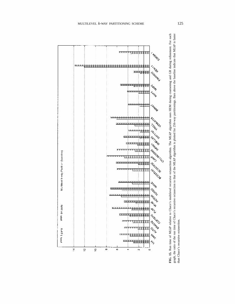
Figure 14 shows the relative performance of our MLkP algorithm compared to Chaco’smultilevel recursive octasection for 8- and 64-way partitionings. Note that for 8-waypartition, no recursive partitioning is performed by Chaco, while for a 64-way partition,only one level of recursion is performed. From this figure we can see that for both 8- and64-way partitioning, MLkP produces partitionings that are in general better than thoseproduced by Chaco’s recursive octasection. For some graphs, MLkP cuts up to 70% feweredges than Chaco does. The difference in quality is due to the following two reasons. First,Chaco’s recursive octasection algorithm uses RM matching during coarsening, whichleads to successive coarser graphs with higher edge-weight. Second, the initial partitioningobtained by spectral octasection is worse (cuts more edges) than the initial partitioningobtained by MLRB. Thus, even though Chaco’s recursive octasection algorithm uses thegeneralized KL refinement algorithm, it does not seem to be able to gain the losses dueto coarsening and initial partitioning. Figure 15 shows the relative run time of Chaco’smultilevel recursive octasection compared to our multilevelk-way partitioning algorithm.From this figure we see that our algorithm is considerably faster. MLkP computes an8-way partitioning about 2 to 6 times faster than Chaco, and a 64-way partitioning about4 to 14 times faster. In summary, for most graphs, MLkP produces better or comparablepartitionings than Chaco’s multilevel recursive octasection in significantly less time. Thisindicates that for most graphs, greedy refinement coupledwith the HEM coarsening and

6Chaco also has recursive bisection scheme that is similar to MLRB.


FIG

.15

.R

untim

eof

MLk

Pre

lativ

eto

Cha

co’s

mul

tilev

elre

curs

ive

octa

sect

ion

algo

rithm

.T

heM

LkP

algo

rithm

uses

HE

Mdu

ring

coar

seni

ngan

dG

Rdu

ring

refin

eme

nt.

For

each

grap

h,th

era

tioof

the

run

time

ofC

haco

’sre

curs

ive

octa

sect

ion

toth

atof

the

MLk

Pal

gorit

hmis

plot

ted

for

256-

way

part

ition

ings

.B

ars

abov

eth

eba

sel

ine

indi

cate

that

MLk

Pis

fast

erth

anC

haco

’sre

curs

ive

octa

sect

ion.


a good initialk-way partition is a much better choice than the computationally expensive8-way Kernighan–Lin refinement.

4. CONCLUSIONS AND DIRECTIONS FORFUTURE RESEARCH

Our experiments have shown that the multilevelk-way partitioning algorithm issignificantly faster than recursive bisection basedk-way partitioning scheme. Thecomplexity of the coarsening and refinement phases of ourk-way partition algorithmis O(|E|), assuming that in each coarsening step the number of vertices is reduced bya factor larger than 1 +ε, whereε is a constant greater than zero. The complexity ofobtaining the initialk-way partitioning of the coarsest graph using MLRB isO(k log k).SinceO(k log k) is often smaller thanO(|E|), the overall complexity of the algorithm isO(|E|). For instance, forTORSOthe run time for a 2-way partitioning is 10.42 s whilethe run time for a 256-way partitioning is only 1.64 times higher (i.e., 17.13 s). As theproblem size increases, this factor decreases. For example, forAUTOthe runtime for a2-way partitioning is 31.03 s while the run time for a 256-way partitioning is only 1.29times higher (i.e., 40 s).

The quality of the partitionings produced by thek-way partitioning algorithm iscomparable or better than that produced by the multilevel recursive bisection algorithm fora wide range of graphs. The scheme works well for a number of reasons. For coarseningheuristics such as HEM and HEM*, the edge-cut of thek-way partitioning produced byMLRB on the coarsest graph is usually within a factor of 1.3 of the final edge-cut. Thisoccurs because the coarsening process creates an excellent smaller replica of the originalgraph, and MLRB finds a very goodk-way partitioning on this small graph. A simplek-way refinement scheme such as GR is able to further improve the initialk-way edge-cut because the refinements needed are fairly local in nature. Hence, the extra power ofgeneralized KL schemes (in terms of its capability of look-ahead) is often unnecessarybecause the refinement needed are fairly local in nature. (In our experiments, the look-ahead capability of GKLR refinement was found useful only for one type of graph.)Furthermore, even a simple refinement scheme such as GR is quite capable of movinglarge portions of graphs across the initialk-way partitioning because the refinement isdone in a multilevel context. For coarse graphs, even a movement of a single vertex atthe partition boundary is equivalent to moving a large number of vertices in the originalgraph. In fact, as discussed in [16], even for MLRB, many simpler variations of theKL refinement algorithm result in equally effective refinement scheme due to the samereason.

Absence of a priority queue in our GR refinement algorithm makes it naturallysuited for parallel implementations. In contrast, the original KL refinement algorithm(and its generalization in thek-way partitioning context) are inherently sequential[6]. In [15] we have developed a highly parallel formulation of our multilevelk-waypartitioning algorithm that uses the vertex-coloring of the successively coarser graph toeffectively parallelize both the coarsening as well as thek-way refinement algorithms.Our experiments on the Cray T3D show that graphs with over a million vertices can bepartitioned in 128 partitions in about 2 s on 128 processors.

An additional advantage of the MLkP algorithm over MLRB is that MLkP is muchmore suited in the context of parallel execution of adaptive computations [25, 26]. Forexample, in adaptive finite element computations, the mesh that models the physical


domain changes dynamically as the simulation progresses. In particular, some parts ofthe mesh become finer and other parts get coarser. Such dynamic adjustments to the meshrequire partitioning of the mesh to improve load balance. This repartitioning also results inmovement of data structures associated with graph vertices. Hence, a good repartitioningalgorithm should minimize the movement of vertices (in addition to balancing the loadand minimizing the cut of the resulting new partition). If started with the multilevelrepresentation of the current partitioning of the graph, ourk-way partitioning refinementalgorithm makes only minor adjustments to the previous partitioning and reduces theoverall movement of vertices and associated data structures.

In all of our experiments, we tried to minimize the edge-cut. However, for manyapplications, minimizing other quantities, such as the number of vertices at the boundaryof the partitions, the number of adjacent partitions, or the shape of the partitions, maybe desirable. This can be accomplished by modifying the refinement algorithm to takeshape of the partitions, may be desirable. This can be accomplished by modifying therefinement algorithm to take into account a different objective function. Even thoughrecursive bisection algorithms can also be modified to use objective functions other thanminimization of edge-cut, the multilevelk-way partitioning algorithm provides a muchbetter framework for this task. This is because multilevelk-way makes it possible toincorporate “global” objective functions that cannot be achieved by recursive bisectionschemes. For example, the overall communication overhead of a processor in parallelsparse matrix–vector multiplication is not proportional to the number of edges thatconnect nonlocal vertices. Actually, it is proportional to the number of vertex valuesit must communicate to neighboring processors. If a vertex on processorPi is connectedto many vertices on processorPj, then the vertex value must be sent to processorPj onlyonce (rather than once for each edge). Hence, the overall communication volume for aprocessor is equal to

∑v Nv, wherev are the boundary vertices in a processor, andNv

is the number of other processors to which vertexv is connected. Note that this metriccan easily be used as the objective function in thek-way partitioning algorithm. But thiscannot be used in recursive bisection-based schemes, because

∑v Nv for each processor

can be computed only in the context of ak-way partition.Thek-way partitioning algorithms described in this paper are available in the METIS 3.0

graph partitioning package that is publicly available on WWW at http://www.cs.umn.edu/∼metis.

REFERENCES

1. S. T. Barnard and H. D. Simon, A fast multilevel implementation of recursive spectral bisection forpartitioning unstructured problems,in “Proceedings of the Sixth SIAM Conference on Parallel Processingfor Scientific Computing,” pp. 711–718, 1993.

2. T. Bui and C. Jones, A heuristic for reducing fill in sparse matrix factorization,in “6th SIAM Conf.Parallel Processing for Scientific Computing,” pp. 445–452, 1993.

3. C.-K. Cheng and Y.-C. A. Wei, An improved two-way partitioning algorithm with stable performance,IEEE Trans. Computer Aided Design10, 12 (Dec. 1991), 1502–1511.

4. C. M. Fiduccia and R. M. Mattheyses, A linear time heuristic for improving network partitions,in “Proc.19th IEEE Design Automation Conference,” pp. 175–181, 1982.

5. J. Garbers, H. J. Promel, and A. Steger, Finding clusters in VLSI circuits,in “Proceedings of IEEEInternational Conference on Computer Aided Design,” pp. 520–523, 1990.


6. J. R. Gilbert and E. Zmijewski, A parallel graph partitioning algorithm for a message-passingmultiprocessor,Int. J. Parallel Program.16 (1987), 498–513.

7. L. Hagen and A. Kahng, Fast spectral methods for ratio cut partitioning and clustering,in “Proceedingsof IEEE International Conference on Computer Aided Design,” pp. 10–13, 1991.

8. L. Hagen and A. Kahng, A new approach to effective circuit clustering, “Proceedings of IEEE InternationalConference on Computer Aided Design,” pp. 422–427, 1992.

9. M. T. Heath and P. Raghavan, A Cartesian parallel nested dissection algorithm,SIAM J. Matrix Anal.

Appl. 16, 1 (1995), 235–253.

10. B. Hendrickson and R. Leland, “An Improved Pectral Graph Partitioning Algorithm for Mapping ParallelComputations,” Technical Report SAND92-1460, Sandia National Laboratories, 1992.

11. B. Hendrickson and R. Leland, “The Chaco User’s Guide,” Version 1.0. Technical Report SAND93-2339,Sandia National Laboratories, 1993.

12. B. Hendrickson and R. Leland, “A Multilevel Algorithm for Partitioning Graphs,” Technical ReportSAND93-1301, Sandia National Laboratories, 1993.

13. G. Karypis and V. Kumar, “Analysis of Multilevel Graph Partitioning,” Technical Report TR 95-037,Department of Computer Science, University of Minnesota, 1995. [Also available on WWW at URLhttp://www.cs.umn.edu/∼karypis] [A short version appears in “Supercomputing ’95”]

14. G. Karypis and V. Kumar, “METIS: Unstructured Graph Partitioning and Sparse Matrix Ordering System,”Technical Report, Department of Computer Science, University of Minnesota, 1995. [Available on WWWat URL http://www.cs.umn.edu/∼karypis/metis]

15. G. Karypis and V. Kumar, “Parallel Multilevelk-way Partitioning Scheme for Irregular Graphs,” TechnicalReport TR 96-036, Department of Computer Science, University of Minnesota, 1996. [Also available onWWW at URL http://www.cs.umn.edu/∼karypis] [A short version appears in “Supercomputing ’96”]

16. G. Karypis and V. Kumar, A fast and highly quality multilevel scheme for partitioning irregular graphs,SIAM J. Sci. Comput.,to appear. [Also available on WWW at URL http://www.cs.umn.edu/∼karypis] [Ashort version appears in “Intl. Conf. on Parallel Processing 1995”]

17. B. W. Kernighan and S. Lin, An efficient heuristic procedure for partitioning graphs,Bell System Tech.

J. 1970.

18. G. L. Miller, S.-H. Teng, W. Thurston, and S. A. Vavasis, Automatic mesh partitioning,in “Sparse MatrixComputations: Graph Theory Issues and Algorithms,” An IMA Workshop Volume, (A. George, J. R.Gilbert, and J. W.-H. Liu, Eds.), Springer-Verlag, New York, 1993.

19. G. L. Miller, S.-H. Teng, and S. A. Vavasis, A unified geometric approach to graph separators,in“Proceedings of 31st Annual Symposium on Foundations of Computer Science,” pp. 538–547, 1991.

20. B. Nour-Omid, A. Raefsky, and G. Lyzenga, Solving finite element equations on concurrent computers,in “American Society of Mechanical Engineering,” (A. K. Noor, Ed.), pp. 291–307, 1986.

21. R. Ponnusamy, N. Mansour, A. Choudhary, and G. C. Fox, Graph contraction and physical optimizationmethods: A quality–cost tradeoff for mapping data on parallel computers,in “International Conferenceof Supercomputing,” 1993.

22. A. Pothen, H. D. Simon, L. Wang, and S. T. Bernard, Towards a fast implementation of spectral nesteddissection,in “Supercomputing ’92 Proceedings,” pp. 42–51, 1992.

23. A. Pothen, H. D. Simon, and K.-P. Liou, Partitioning sparse matrices with eigenvectors of graphs,SIAM

J. Matrix Anal. Appl.11, 3 (1990), 430–452.

24. P. Raghavan, “Line and Plane Separators,” Technical Report UIUCDCS-R-93-1794, Department ofComputer Science, University of Illinois, Urbana, IL 61801, Feb. 1993.

25. K. Schloegel, G. Karypis, and V. Kumar, Multilevel diffusion algorithms for repartitioning of adaptivemeshes,J. Parallel Distrib. Comput.47, No. 2 (1997).

26. K. Schloegel, G. Karypis, and V. Kumar, Repartitioning of adaptive meshes: Experiments with multileveldiffusion, in “Proceedings of the Third International Euro-Par Conference,” pp. 945–949, Aug. 1997.

27. H. D. Simon and S.-H. Teng, “How Good is Recursive Bisection?,” Technical Report RNR-93-012, NASSystems Division, Moffet Field, CA, 1993.


GEORGE KARYPIS received his Ph.D. in computer science at the University of Minnesota, and he iscurrently an assistant professor at the Department of Computer Science and Engineering at the University ofMinnesota. His research interests span the areas of parallel algorithm design, applications of parallel processingin scientific computing and optimization, sparse matrix computations, parallel programming languages andlibraries, and data mining. His recent work has been in the areas of parallel sparse direct solvers, serial andparallel graph partitioning algorithms, parallel matrix ordering algorithms, and scalable parallel preconditioners.His research has resulted in the development of software libraries for unstructured mesh partitioning (METISand ParMETIS) and for parallel Cholesky factorization (PSPASES). He is the author of over 20 research articlesand a coauthor of the widely used text book “Introduction to Parallel Computing.”

VIPIN KUMAR received his Ph.D. in computer science at the University of Maryland, and he is currently aprofessor at the Department of Computer Science and Engineering at the University of Minnesota. His currentresearch interests include parallel computing, parallel algorithms for scientific computing problems, and datamining. His research has resulted in the development of highly efficient parallel algorithms and software forsparse matrix factorization (PSPASES), graph partitioning (METIS and ParMETIS), and dense hierarchicalsolvers. Kumar’s research in performance analysis resulted in the development of the isoefficiency metric foranalyzing the scalability of parallel algorithms. He is the author of over 100 research articles and a coauthorof the widely used text book “Introduction to Parallel Computing.” Kumar has given over 50 invited talksat various conferences, workshops, and national labs and has served as chair/co-chair for many conferences/workshops in the area of parallel computing. Kumar serves on the editorial boards ofIEEE Parallel andDistributed Technology, IEEE Transactions of Data and Knowledge Engineering, Parallel Computing, and theJournal of Parallel and Distributed Computing. He is a senior member of IEEE and a member of SIAMand ACM.

Received November 1, 1996; revised October 15, 1997; accepted October 20, 1997

Documents

Multilevel k-way Partitioning Scheme for Irregular Graphs