Embed Size (px)
Citation preview

MULTILEVEL FIRST-ORDER SYSTEM LEAST SQUARES FORELLIPTIC GRID GENERATION
A. L. CODD∗, T. A. MANTEUFFEL† , S. F. MCCORMICK†, , AND J. W. RUGE†
Abstract. A new fully-variational approach is studied for elliptic grid generation (EGG). Itis based on a general algorithm developed in a companion paper [10] that involves using Newton’smethod to linearize an appropriate equivalent first-order system, first-order system least squares(FOSLS) to formulate and discretize the Newton step, and algebraic multigrid (AMG) to solve theresulting matrix equation. The approach is coupled with nested iteration to provide an accurate initialguess for finer levels using coarse-level computation. The present paper verifies the assumptions of[10] and confirms the overall efficiency of the scheme with numerical experiments.
Key words. least-squares discretization, multigrid, nonlinear elliptic boundary value problems
AMS subject classifications. 35J65, 65N15, 65N30, 65N50, 65F10
1. Introduction. A companion paper [10] develops an algorithm using Newton’smethod, first-order system least squares (FOSLS), and algebraic multigrid (AMG)for efficient solution of general nonlinear elliptic equations. The equations are firstconverted to an appropriate first-order system and an approximate solution to thecoarsest-grid problem is then computed (by any suitable method such as Newtoniteration coupled with perhaps direct solvers, damping, or continuation). The ap-proximation is then interpolated to the next finer level where it is used as an initialguess for one Newton linearization of the nonlinear problem, with a few AMG cyclesapplied to the resulting matrix equation. This algorithm repeats itself until the finestgrid is processed, again by one Newton/AMG step. At each Newton step, FOSLS isapplied to the linearized system and the resulting matrix equation is solved using justa few V-cycles of AMG.
In the present paper, we apply this algorithm to the elliptic grid generation (EGG)equations. Grid generation is usually based on a map between a relatively simplecomputational region and a possibly complicated physical region. It can be usednumerically to create a mesh for a discretization method to solve a given system ofequations posed on the physical domain. Alternatively, it can be used to transformequations posed on the physical region to ones posed on the computational region,where the transformed equations are then solved. If the Jacobian of the transformationis positive throughout the computational region, the equation type is unchanged [12].Actually, the relative minimum value of the Jacobian is important in practice becauserelatively small values signal small angles between the grid lines and large errors inapproximating the equations [20].
Our interest is in elliptic grid generation using the Winslow generator [12], whichallows us to specify the boundary maps completely. Moreover, by choosing the two-dimensional computational region to be convex, we can ensure that the Jacobian ofthe map is positive, which in turn ensures that the map is one-to-one and onto and
∗Centre for Mathematics and Its Applications, School of Mathematical Sciences, Australian Na-tional University, Canberra, ACT 0200, Australia. email: [email protected].,
†Department of Applied Mathematics, Campus Box 526, University of Colorado at Boulder,Boulder, CO 80309–0526. email: [email protected], [email protected],and [email protected]. This work was sponsored by the National Institute of Health undergrant number 1–R01–EY12291–01, the National Science Foundation under grant number DMS–9706866, and the Department of Energy under grant number DE–FG03–93ER25165.,
1

2
therefore does not fold [8]. The Winslow generator tends to create smooth grids, withgood aspect ratios. The map also tends to control variations in gridline spacing andnonorthogonality of the gridline intersections in the physical space. See Thompson,Warsi, and Mastin [20] and Knupp and Steinberg [12] for background on grid gener-ation in general, and EGG in particular. Several discretization methods of the EGGequations together with their associated errors are discussed in [20]. In [12], the EGGequations are derived and several existing methods are described for solving them.
A brief description of the first-order EGG system is given in section 2. Theassumptions needed to apply the theory in [10] are verified in section 3. Section 4discusses scaling of the functional terms used for the computations as well as numericalresults for two representative problems. The last section includes some final remarks.
2. Equations. We use standard notation for the associated spaces. Restrictingourselves to two dimensions, consider a generic open domain, Ω ∈ R2, with Lipschitzboundary Γ ∈ C3,1. (Superscript 1 indicates Lipschitz continuity of the functions andtheir derivatives.) Suppose m ≥ 0 and n ≥ 1 are given integers. Let (·, ·)0,Ω denotethe inner product on L2(Ω)n, ‖ · ‖0,Ω its induced norm, and Hm(Ω)n the standardSobolev space with norm ‖ · ‖m,Ω and seminorms | · |i,Ω (0 ≤ i ≤ m). (Superscript n isomitted when dependence is clear by context.) For δ ∈ (0, 1), let Hm+δ(Ω) (c.f. [6])denote the Sobolev space associated with the norm defined by
‖u‖2m+δ,Ω ≡ ‖u‖2
m,Ω +∑
|α|=m
∫Ω
∫Ω
|∂αu(x) − ∂αu(y)|2|x − y|2(1+δ)
dxdy.
(This definition allows the use of the ”real interpolation” method [1, 6].) Also, letH
12 (Γ) denote the trace Sobolev space associated with norm
‖u‖ 12 ,Γ ≡ inf‖v‖1,Ω : v ∈ H1(Ω), trace v = u on Γ.
We start by mapping a known convex computational region, Ω ∈ R2 with bound-ary Γ ∈ C3,1 to a given physical region, Ωx ∈ R2 with boundary Γx ∈ C3,1. We definemap ξ : Ωx → Ω and its inverse, x : Ω → Ωx. The coordinates in Ωx are denoted bythe vector of unknowns x = (x y)t and those in Ω by ξ = (ξ η)t.
For the EGG smoothness or Winslow generator, we choose ξ to be harmonic:
∆ξ = 0,ξ = v(x),
in Ωx,on Γx,
(2.1)
where v ∈ H72 (Γx) is a given homeomorphism (continuous and one-to-one) from
the boundary of the physical region onto the boundary of the computational region.(H
72 (Γx) is consistent with our boundary smoothness assumption, Γ ∈ C3,1.) With Ωx
bounded, the weak form of Laplace system (2.1) has one and only one solution, ξ∗, inH4(Ωx)2 [11] and, by Weyl’s Lemma [22], ξ∗ ∈ C∞
loc(Ωx) ≡ ξ ∈ C∞(K) , ∀ K ⊂ Ωx.Map ξ∗ is posed on Ωx, so computing an approximation to it would nominally
involve specifying a grid on the physical region. But specifying such a grid is theaim of EGG in the first place, so this formulation is not useful. We therefore chooseinstead to solve the inverse of problem (2.1), which takes a regular grid in Ω and mapsit onto a grid in Ωx, thus achieving our objective. To this end, we assume Ωx and Ω tobe simply connected and bounded and Ω to be convex, so Γ and Γx are simple closedcurves. Map ξ∗ is continuous and harmonic and v is a homeomorphism of Γx ontoΓ, so Rado’s Theorem (c.f. [16]) implies existence of a unique inverse map, x∗, from

3
Ω onto Ωx. An outline of the proof is provided in [14]. It then follows that domainmap ξ∗ is a diffeomorphism [8, 12] and the associated Jacobian, J∗
x ≡ ξ∗xν∗y − ξ∗yν∗
x, iscontinuous and uniformly positive and bounded on Ωx (J0 ≤ |J∗
x(x, y)| ≤ J1 for someconstants J0, J1 ∈ R+ and all (x, y) ∈ Ωx). The choice for the space for x∗ followsfrom the assumptions for ξ∗, Γx, and v, and is discussed further in section 3.
The inverse map satisfies the following equations (positive Jacobian throughoutΩx ensures that the solution of (2.1) is an invertible map):
(x2η + y2
η)xξξ − (xξxη + yξyη)(xξη + xηξ) + (x2ξ + y2
ξ )xηη = 0, in Ω,
(x2η + y2
η)yξξ − (xξxη + yξyη)(yξη + yηξ) + (x2ξ + y2
ξ )yηη = 0, in Ω,
x = w1(ξ, η), on Γ,y = w2(ξ, η), on Γ,
(2.2)
where function w =(
w1(ξ, η)w2(ξ, η)
)is the inverse of function v =
(v1(x, y)v2(x, y)
)(i.e., x =
w(v(x))). See [12] for more detail. The inverse map, x∗, exists and solves (2.2).We assume that the Frechet derivative of the operator in (2.2) at x∗ is one-to-oneon H2+δ
0 (Ω)2 (subscript 0 denoting homogeneous Dirichlet conditions on Γ). This iseasily verified when x∗ deviates from a constant map by a sufficiently small amount.
To apply our method, we begin by converting equations (2.2) to a first-ordersystem. We could write these equations in a simple way using the standard notationof a 2× 2 matrix for the Jacobian matrix, but this is not convenient for the linearizedequations treated section 3. Our notation is therefore based primarily on writing theJacobian matrix as a 4 × 1 vector:
J =
xξ
xη
yξ
yη
=
J11
J21
J12
J22
.
On the other hand, at times it is useful to refer to the matrix form of the unknowns.We therefore define the block-structured matrix J and its classical adjoint J as follows:
J =
J11 J21 0 0J12 J22 0 00 0 J11 J21
0 0 J12 J22
and J =
J22 −J21 0 0−J12 J11 0 0
0 0 J22 −J21
0 0 −J12 J11
.
Note that the Jacobian of the inverse transformation is given by
J ≡ xξyη − xηyξ = J11J22 − J21J12 =√
detJ.
Also, J = 1Jx
and ‖J‖∞,Ω = ‖ 1Jx
‖∞,Ωx = 1‖Jx‖∞,Ωx
> 0.In keeping with the vector notation, denote grad, div, and curl, respectively, by
∇ =
∂ξ 0∂η 00 ∂ξ
0 ∂η
,∇· =(∂ξ ∂η 0 00 0 ∂ξ ∂η
),∇× =
(−∂η ∂ξ 0 0
0 0 −∂η ∂ξ
).
The same calculus notation is used in both Ωx and Ω (e.g., ∇, ∇·, and ∇×). Differ-entiation in Ωx is with respect to x and y and differentiation in Ω is with respect to

4
ξ and η. Let the boundary unit normal vector be denoted by
n =
n1 0n2 00 n1
0 n2
.(2.3)
As in previous applications of the FOSLS methodology (c.f. [7]), the natural first-order system is often augmented with a curl equation to ensure that the system iselliptic in the H1 product norm. The augmented system also allows for the possibilityof solving for the unknowns in two separate stages: we can solve for J alone in thefirst stage, then fix J and solve for x alone in the second stage, as the followingdevelopment shows. The curl-augmented system we consider here is
J −∇x = 0, in Ω,
(JJt∇) · J = 0, in Ω,∇× J = 0, in Ω,
x = w, on Γ,n × J = n ×∇w, on Γ.
(2.4)
To be very clear about our notation, note that derivatives only apply to terms on theirright. Thus, for (JJ
t∇)· in the second equation of (2.4), the matrix multiplication isapplied first, keeping the order of each entry in the resulting matrix consistent withthe multiplication. To perform the dot product, the matrix is transposed withoutaltering the order of the terms in each component. For example, if we write
JJt=
α −β 0 0−β γ 0 00 0 α −β0 0 −β γ
,
then
(JJt∇) · J =
(α∂J11
∂ξ − β ∂J11∂η − β ∂J21
∂ξ + γ ∂J21∂η
α∂J12∂ξ − β ∂J12
∂η − β ∂J22∂ξ + γ ∂J22
∂η
).
We consider a two-stage algorithm, but focus only on the following first stage:
(JJt∇) · J = 0, in Ω,∇× J = 0, in Ω,n × J = n ×∇w, on Γ.
(2.5)
Note that x can be recovered from the solution of (2.5) by a second stage that mini-mizes ‖∇x−J‖2
0,Ω +‖x−w‖212 ,Γ
over x with the computed J held fixed. The homoge-
neous part of the first term in this functional is precisely the H1(Ω)4 seminorm of x,so minimizing this functional leads to a simple system of decoupled Poisson equations.The remainder of our analysis therefore focuses on (2.5).
To obtain homogeneous boundary conditions, we rewrite the equations in termsof the perturbation, D, of a smooth extension of w into Ω. To this end, suppose thatsome function w ∈ H4(Ω)2 is given so that its trace agrees with w on Γ. DefiningE ≡ ∇w ∈ H3(Ω)4, we thus have
n × E = n ×∇w, on Γ.(2.6)
5
(In practice, we do not really need an extension of w, but rather just an extension ofits gradient: any E ∈ H3(Ω)4 that satisfies (2.6) will do. However, if this extension isnot necessarily a gradient, then E must be included in the curl term in (2.7) below.)
In the notation of the companion paper [10], we have
P(D) ≡((
(E + D)(E + D)t∇)· (E + D)
∇× D
)= 0,(2.7)
with boundary conditions
n × D = 0.(2.8)
System (2.7)-(2.8) corresponds to the inverse Laplace problem with Dirichlet bound-ary conditions. Existence of a solution, D∗, that yields a positive Jacobian is guaran-teed by Rado’s theorem. We show in section 3 that D∗ ∈ H3(Ω)4. One implicationof this smoothness property is that (E+ D
∗)(E+ D
∗)t is a uniformly positive definite
and bounded matrix on Ω.From the companion paper [10], we define
H1+δ ≡ D ∈ H1+δ(Ω)4 : n × D = 0 on Γ.
Restricting D to H1+δ(Ω)4 ensures that((E + D)(E + D)t∇
)· (E + D) ∈ L2(Ω)2,
as the results of the next section show.The first Frechet derivative of (2.7) in direction K is
P′(D)[K] =
(((D + E)(D + E)t∇
)· K + B · K
∇× K
),(2.9)
where
B · K ≡(K(D + E)t∇
)· (D + E) +
((D + E)K
t∇)· (D + E).
and the second Frechet derivative in directions K and M is
P′′(D)[K,M] =
((M(D + E)t∇
)· K +
((D + E)M
t∇)· K
0
)
+
((K(D + E)t∇
)· M +
((D + E)K
t∇)· M
0
)(2.10)
+
((KM
t∇)· (D + E) +
(MK
t∇)· (D + E)
0
).
3. The Assumptions and their Verification. Consider the assumptions madein companion paper [10]. The first is existence of a solution in H2+δ. From [16], weknow that a unique inverse map exists and that it provides a solution, D∗, to (2.7).Recall that ξ∗ ∈ H4(Ωx)2. In lemma 3.4 below, we show that D∗ ∈ H3. Thisestablishes our first assumption for the EGG equations for any δ ∈ (0, 1).
The remaining assumptions we need to establish are, for ε = 0 or δ, that P[D] ∈Hε(Ω)4 for every D ∈ Br (lemma 3.5), that ‖P′(D)[ · ]‖ε,Ω is H1+ε(Ω)4 equivalent(lemma 3.6), and that the second Frechet derivative of P(D) is bounded for all D ∈ Br

6
(lemma 3.7). (The discretization assumptions are standard.) But first we need threeresults that follow directly from a corollary to the Sobolev Embedding theorem [11],which (tailored to our needs) states that the product of a function in Hm1(Ω) and afunction in Hm2(Ω) is in Hm(Ω) provided that either m1 + m2 − m ≥ 1, m1 > m,and m2 > m or m1 + m2 − m > 1, m1 ≥ m, and m2 ≥ m.
Assume that r > 0 is so small that matrix (E + D)(E + D)t is positive definiteand bounded uniformly on Ω and over D ∈ Br ≡ D ∈ H1+δ : ‖D∗ − D‖1+δ,Ω < r.This assumption is possible because it is true at D = D∗ and because the matrixis continuous as a function defined on Br. Assume that a, b, c ∈ H1+δ(Ω). Forconvenience, we let ∂ denote either ∂x or ∂y. In the proof of lemma 3.4, we also use∂2 to denote any of the four second partial derivatives and ∂3 for any combination ofthird partial derivatives. Note that (∂a)2 could mean axay, for example.
Lemma 3.1. There exists a constant, C, depending only on Ω and δ, such that
‖ab∂c‖ε,Ω ≤ C‖a‖1+δ,Ω‖b‖1+δ,Ω‖c‖1+ε,Ω
Proof. Using the corollary to the Sobolev Imbedding theorem [11] with m1 =1 + δ, m2 = ε, and m = ε twice yields
‖ab∂c‖ε,Ω ≤ C‖a‖1+δ,Ω‖b∂c‖ε,Ω
≤ C‖a‖1+δ,Ω‖b‖1+δ,Ω‖∂c‖ε,Ω
≤ C‖a‖1+δ,Ω‖b‖1+δ,Ω‖c‖1+ε,Ω.
Lemma 3.2. There exists a constant, C, depending only on Ω and δ, such that
‖ab∂c‖ε,Ω ≤ C‖a‖1+δ,Ω‖b‖1+ε,Ω‖c‖1+δ,Ω
Proof. Using the corollary to the Sobolev imbedding theorem [11] first withm1 = 1 + δ, m2 = ε, and m = ε, then with m1 = 1 + ε, m2 = δ, and m = ε yields
‖ab∂c‖ε,Ω ≤ C‖a‖1+δ,Ω‖b∂c‖ε,Ω
≤ C‖a‖1+δ,Ω‖b‖1+ε,Ω‖∂c‖δ,Ω
≤ C‖a‖1+δ,Ω‖b‖1+ε,Ω‖c‖1+δ,Ω.
Lemma 3.3. Assume that a, b ∈ H2+δ(Ω) and k ∈ H1+δ(Ω). Then there exists aconstant, C, depending only on Ω and δ, such that
‖ak∂b‖1,Ω ≤ C‖a‖1+δ,Ω‖b‖2+δ,Ω‖k‖1,Ω.
Proof.
‖ak∂b‖1,Ω ≤ C‖a‖1+δ,Ω‖k∂b‖1,Ω
≤ C‖a‖1+δ,Ω‖∂b‖1+δ,Ω‖k‖1,Ω
≤ C‖a‖1+δ,Ω‖b‖2+δ,Ω‖k‖1,Ω,
where we used corollary to the Sobolev imbedding theorem from [11] with m1 =1 + δ, m2 = 1, and m = 1 twice.

7
Lemma 3.4. The solution, D∗, of (2.7) is in H3(Ω)4.Proof. We have
J∗ ≡ E + D∗ =
J∗
11
J∗21
J∗12
J∗22
=
x∗
ξ
x∗η
y∗ξ
y∗η
=1J∗x
η∗
y
−ξ∗y−η∗
x
ξ∗x
,
where E ∈ H3(Ωx)4 and ξ∗ ∈ H4(Ωx)2. We now show that J∗ ∈ H3(Ω)4, from whichfollows the result that D∗ ∈ H3(Ω)4.
Since ξ∗ ∈ H4(Ωx)2, then ξ∗x, ξ∗y , η∗x, η∗
y ∈ H3(Ωx). From the corollary to theSobolev imbedding theorem (with m1 = 3, m2 = 3, and m = 3), we must haveJ∗x = ξ∗xη∗
y − ξ∗yη∗x ∈ H3(Ωx). Recall from section 2 that J∗ is continuous and
uniformly positive and bounded: J0 ≤ |J∗x(x, y)| ≤ J1 for some constants J0, J1 ∈ R+
and all (x, y) ∈ Ωx.Dropping superscript ∗ for convenience, consider J11. (The other entries are
treated similarly.) Using the corollary to the Sobolev imbedding theorem [11] withm1 = 3, m2 = 3, and m = 3, we get
‖J11‖3,Ω =∥∥∥∥ 1
Jxηy
∥∥∥∥3,Ωx
≤ C
∥∥∥∥ 1Jx
∥∥∥∥3,Ωx
‖ηy‖3,Ωx.
Therefore, we need only show that 1Jx
∈ H3. But∥∥∥∥ 1Jx
∥∥∥∥2
3,Ωx
=∑i≤3
∥∥∥∥∂i 1Jx
∥∥∥∥2
0,Ωx
.
We consider each order separately. By theorem 3.2 in [21], for any a ∈ C0(Ωx) andb ∈ L2(Ωx), we have
‖ab‖0,Ωx ≤ ‖a‖∞,Ωx‖b‖0,Ωx .(3.1)
For the zeroth-order term, using (3.1) yields∥∥∥∥ 1Jx
∥∥∥∥0,Ωx
≤∥∥∥∥ 1
Jx
∥∥∥∥∞,Ωx
‖1‖0,Ωx ≤ 1J0
‖1‖0,Ωx .
For the first-order term, we use (3.1) to get∥∥∥∥∂1Jx
∥∥∥∥0,Ωx
=∥∥∥∥−1
J2x
∂Jx
∥∥∥∥0,Ωx
≤ 1J2
0
‖∂Jx‖0,Ωx≤ 1
J20
‖Jx‖1,Ωx.
For the second-order term, we use the triangle inequality, (3.1), and the Corollaryto the Sobolev imbedding theorem with m1 = m2 = 1 and m = 0 to get∥∥∥∥∂2 1
Jx
∥∥∥∥0,Ωx
=∥∥∥∥ 2
J3x
(∂Jx)2 +−1J2x
∂2Jx
∥∥∥∥0,Ωx
≤∥∥∥∥ 2
J3x
(∂Jx)2∥∥∥∥
0,Ωx
+∥∥∥∥ 1
J2x
∂2Jx
∥∥∥∥0,Ωx
≤ 2J3
0
∥∥(∂Jx)2∥∥
0,Ωx+
1J2
0
∥∥∂2Jx
∥∥0,Ωx

8
≤ C
(2J3
0
‖∂Jx‖21,Ωx
+1J2
0
‖Jx‖2,Ωx
)≤ C
(2J3
0
‖Jx‖22,Ωx
+1J2
0
‖Jx‖2,Ωx
).
For the third-order term, we use the triangle inequality, (3.1), and the Corollaryto the Sobolev imbedding theorem once with m1 = 1, m2 = 3
4 , and m = 0, once withm1 = m2 = 1 and m = 0, and once with m1 = m2 = 1 and m = 3
4 to get∥∥∥∥∂3 1Jx
∥∥∥∥0,Ωx
=∥∥∥∥−6
J4x
(∂Jx)3 +6J3x
∂Jx∂2Jx +−1J2x
∂3Jx
∥∥∥∥0,Ωx
≤∥∥∥∥ 6
J4x
(∂Jx)3∥∥∥∥
0,Ωx
+∥∥∥∥ 6
J3x
∂Jx∂2Jx
∥∥∥∥0,Ωx
+∥∥∥∥ 1
J2x
∂3Jx
∥∥∥∥0,Ωx
≤ 6J4
0
∥∥(∂Jx)3∥∥
0,Ωx+
6J3
0
∥∥∂Jx∂2Jx
∥∥0,Ωx
+1J2
0
∥∥∂3Jx
∥∥0,Ωx
≤ C
(6J4
0
‖∂Jx‖31,Ωx
+6J3
0
‖∂Jx‖1,Ωx
∥∥∂2Jx
∥∥1,Ωx
+1J2
0
‖Jx‖3,Ωx
)≤ C
(6J4
0
‖Jx‖32,Ωx
+6J3
0
‖Jx‖2,Ωx‖Jx‖3,Ωx
+1J2
0
‖Jx‖3,Ωx
).
The result follows from these bounds.Lemma 3.5. P[D] ∈ Hε(Ω)p for every D ∈ Br: there exists a constant, C,
depending only on D∗, E, r, Ω, and δ, such that
‖P(D)‖ε,Ω ≤ C, ∀ D ∈ Br.(3.2)
Proof. The products in (2.7) are of the form treated in lemma 3.1. In fact, thereexists a constant, C, depending only on Ω and δ, such that
‖P(D)‖ε,Ω ≤ C(‖D + E‖21+δ,Ω‖D + E‖1+ε,Ω + ‖D‖1+ε,Ω),(3.3)
so (3.2) follows because D ∈ Br.Next we establish uniform coercivity and continuity of P′ in a neighborhood of
D∗. This result needs the assumption that P′(D∗)[ · ] is one-to-one on H1+δ, whichis a consequence of an analogous assumption on the original EGG equations.
Lemma 3.6 (Ellipticity Property). ‖P′(D)[ · ]‖ε,Ω is H1+ε(Ω)4 equivalent: thereexists constants cc and cb, depending only on D∗,E, r,Ω, and δ, such that
1cc‖K‖1+ε,Ω ≤ ‖P′(D)[K]‖ε,Ω ≤ cb‖K‖1+ε,Ω, ∀ K ∈ H1+ε.(3.4)
Proof. The products in (2.9) are of the form treated in lemmas 3.1 and 3.2. Infact, there exists a constant, C, depending only on Ω and δ, such that
‖P′(D)[K]‖ε,Ω ≤ C(‖D + E‖21+δ,Ω‖K‖1+ε,Ω + ‖K‖1+ε,Ω).(3.5)
Proof of the lower bound follows from theorem 10.5 of ADN2 [2] as we now show.We first need to prove Hm+1 boundedness and coercivity for P′(D∗)[K]: there existsconstants, c1 and c3, depending only on D∗,E, m, and Ω, such that
1c1
‖K‖m+1,Ω ≤ ‖P′(D∗)[K]‖m,Ω ≤ c3‖K‖m+1,Ω, ∀ K ∈ Hm+1,(3.6)

9
for any m ∈ [0, 1]. The upper bound is simply an application of the corollary tothe Sobolev imbedding theorem similar to lemmas 3.1 and 3.2. Consider the lowerbound. It would be a simple matter to just assume D∗ ∈ H3+δ and then, becausethe coefficients would be sufficiently smooth, apply ADN2 theory for both m = 0 andm = 1. Instead, we just have D∗ ∈ H2+δ, so while the higher-order coefficients are inC1, the lower order coefficients are only in C0. This means that we need more care.
First consider m = 0. What follows for this case is a straightforward applicationof ADN2 theory to the entire system because all of the coefficients are sufficientlysmooth. Recall that Ω is a bounded open subset of R2 with C3,1 boundary Γ. Wewrite the system as
LK = f , in Ω,BK = g, on Γ,
(3.7)
where L ≡ P′(D∗) and B = n×. (Recall that n is the outward unit normal on Γ(2.3).) For convenience, we write the coefficients using J∗ = D∗ + E and drop the ∗
from the components. Note that L = L1 + L2 and lij = l′ij + l′′ij , where
L1 = (l′ij(ξ, ∂)) =
α∂ξ − β∂η −β∂ξ + γ∂η 0 0
0 0 α∂ξ − β∂η −β∂ξ + γ∂η
−∂η ∂ξ 0 00 0 −∂η ∂ξ
,
L2 = (l′′ij(ξ, ∂))
=
2J11J21,η − J21(J11,η + J21,ξ) 2J11J22,η − J21(J12,η + J22,ξ) 0 02J21J11,ξ − J11(J11,η + J21,ξ) 2J21J12,ξ − J11(J12,η + J22,ξ) 0 02J12J21,η − J22(J11,η + J21,ξ) 2J12J22,η − J22(J12,η + J22,ξ) 0 02J22J11,ξ − J12(J11,η + J21,ξ) 2J22J12,ξ − J12(J12,η + J22,ξ) 0 0
t
,
α = J221 + J2
22, β = J11J21 + J12J22, γ = J211 + J2
12.
Note that
B = (bij(ξ, ∂)) =(−n2 n1 0 00 0 −n2 n1
).(3.8)
In ADN2 theory, three types of integer weights are used to determine the leading-order terms for boundary value problem (3.7). Weight si ≤ 0 refers to the ith equation,weight tj ≥ 0 to the jth dependent variable, and weight rk to the kth boundarycondition. These weights are chosen as small as possible but so that
deg lij(ξ, ∂) ≤ si + tj , deg bkj(ξ, ∂) ≤ rk + tj , i, j = 1, 2, 3, 4, k = 1, 2,
where deg refers to the order of the derivatives. Our weights are
si = 0, tj = 1, rk = −1, i, j = 1, 2, 3, 4, k = 1, 2.
The leading-order part of L consists of the elements lij for which deg lij(ξ, ∂) =si + tj = 1. Therefore, L1 is the leading-order (in this case, first-order) part. Theleading-order part of B consists of elements bkj for which deg bkj(ξ, ∂) = rk + tj = 0.Therefore, the leading-order (in this case, zeroth-order) part of B is B itself.

10
We must show that L1 satisfies two ADN2 conditions: the Supplementary Con-dition on its determinant and uniform ellipticity. (L1 will then automatically beelliptic.) ADN2 also requires that the system of equations and boundary conditionsbe well-posed. This means that L1 and B, when combined, must satisfy the Comple-menting Boundary Condition. Let L denote the determinant of L1:
L(ξ, ∂) = det(l′ij) = −(α∂2ξ − 2β∂ξ∂η + γ∂2
η)2.
Since J > 0 (see section 2), then
β2 − αγ = (xξxη + yξyη)2 − (x2η + y2
η)(x2ξ + y2
ξ )= −(xξyη − yξxη)2 = −J2 < 0.
(3.9)
Let d = (d e)t and p = (p q)t be any two linearly independent vectors. To aidclarity of the following discussion, we first define some quantities:
A = αdp − β(pe + dq) + γeq,
B =√DC −A2 = J |pe − dq|,
C = αd2 − 2βde + γe2,D = αp2 − 2βpq + γq2.
Note that B > 0 since J > 0 and linear independence of p and d implies |pe−dq| > 0.The Supplementary Condition on L requires the equation
L (ξ,d + τp) = −C + 2τA + τ2D2 = 0(3.10)
to have exactly two roots in τ with positive imaginary part. Polynomial (3.10) hastwo double roots (ι =
√−1),
τ =−A± ιB
D ,
which form two complex conjugate pairs. Thus, (3.10) does indeed have exactly tworoots with positive imaginary part (one such double root).
To satisfy uniform ellipticity, we need to show that
1C‖d‖4 ≤ |L (ξ,d)| ≤ C‖d‖4,(3.11)
with ‖d‖ =√
d2 + e2, for all vectors d = 0 and points ξ in Ω.To prove the left bound in (3.11), let ρ = |β|√
αγ < 1 (see (3.9)). Then
|L (ξ,d)| = (αd2 − 2βde + γe2)2
≥ (αd2 − 2|β||d||e| + γe2)2
= (αd2 − 2ρ√
αγ|d||e| + γe2)2
= ((1 − ρ)(αd2 + γe2) + ρ(√
αd −√γe)2)2
≥ ((1 − ρ)(αd2 + γe2))2
≥ min((1 − ρ)2α2, (1 − ρ)2γ2)(d2 + e2)2
= min((1 − ρ)2α2, (1 − ρ)2γ2)‖d‖4.
To prove the right bound in (3.11), note that Holder’s inequality implies that
|L (ξ,d)| ≤ (αd2 + 2|β||d||e| + γe2)2
≤ (αd2 + |β|(d2 + e2) + γe2)2
≤ max((α + |β|)2, (γ + |β|)2)(d2 + e2)2
= max((α + |β|)2, (γ + |β|)2)‖d‖4.

11
We then establish (3.11) by choosing
C = max
1(1 − ρ)2α2
,1
(1 − ρ)2γ2, (α + |β|)2), (γ + |β|)2)
.
This shows that operator L satisfies the two conditions of ADN2. We now provethat the problem is well-posed by showing that L1 and B satisfy the ComplementingBoundary Condition. This condition involves comparing of two polynomials. We con-sider a point on the boundary with normal d = (d e)t and tangent p = (p q)t vectors.The first polynomial is formed from the roots of (3.10) with positive imaginary parts:
M+(ξ,d, τ) =[τ +
A− ιBD
]2
.(3.12)
The second polynomial is formed from the leading order elements of L and B:2∑
k=1
ak(BL)km,(3.13)
where
(BL)km =4∑
j=1
bkj(ξ,d + τp)ljm(ξ,d + τp),
and ljm(ξ,d+ τp) are the elements of the (classical) adjoint (l′ij ljm = δm
i L, i, j, m =1, 2, 3, 4) of l′ij(ξ,d + τp) and bkj is defined in (3.8).
The polynomials for (3.13) are
(2∑
k=1
ak(BL)km
)= D
[τ +
A + ιBD
] [τ +
A− ιBD
]a1(pe − qd)a2(pe − qd)a1(A + τD)a2(A + τD)
t
.(3.14)
Comparing polynomials (3.12) and (3.14) and noting that B > 0, we have that (3.12)is not a factor of (3.14). Thus, the Complementing Boundary Condition is satisfied.
Theorem 10.5 from ADN2 [2] implies that, for lij ∈ Cm(Ω), bkj ∈ Cm+1(Γ), thereexists a constant, c1, that depends only on D∗,E, r,Ω and δ, such that, if Kj ∈ H1(Ω),1 ≤ j ≤ 4, solves (3.7) and is unique, then Kj ∈ Hm+1(Ω) and
‖Kj‖m+1,Ω ≤ c1
4
[4∑
i=1
‖fi‖m,Ω +2∑
i=1
‖gi‖m+ 12 ,Γ
],
where fi and gi are the components of f and g, respectively, in (3.7). The coefficients ofL are at least in H1+δ(Ω) and C0(Ω). For the boundary conditions, we have B = n×and Γ ∈ C3,1, so we get bkj ∈ C2(Γ). The boundary conditions are homogeneous, sowe can drop the boundary term in the inequality. We therefore have
‖K‖1,Ω ≤ c1‖L(D∗)[K]‖0,Ω, ∀ K ∈ H1(Ω)4.(3.15)
Now consider m = 1. We cannot simply apply ADN2 to the whole system becausethe coefficients are not sufficiently smooth. Instead, we split the operator accordingto L = L1 + L2 and restrict our ADN2 result to reduced system
L1K = f , in Ω,BK = g, on Γ.

12
Operator L1 satisfies the ADN2 conditions (as illustrated for case m = 0), so
‖K‖2,Ω ≤ c1‖L1(D∗)[K]‖1,Ω, ∀ K ∈ H2.(3.16)
The coefficients of L1 are in H2+δ(Ω) and C1(Ω). For the boundary conditions, wehave B = n× and Γ ∈ C3,1, so we get bkj ∈ C2(Γ). The boundary conditions arehomogeneous, so we can drop the boundary term in the inequality.
We use lemma 3.3 to obtain
‖L2(D∗)[K]‖1,Ω ≤ c2‖K‖1,Ω, ∀ K ∈ H2.(3.17)
Note that c2 depends continuously on supD∈Br‖D∗ + E‖2+δ,Ω, so it depends on
D∗,E, r, Ω, and δ.Combining (3.16) and (3.17) yields
‖K‖2,Ω ≤ C(‖P′(D∗)[K]‖1,Ω + ‖K‖1,Ω), ∀ K ∈ H2.(3.18)
This is a Gardings inequality (cf. [13, 19]), which allows us now to prove that
1cc‖K‖2,Ω ≤ ‖P′(D∗)[K]‖1,Ω, ∀ K ∈ H2.(3.19)
To this end, assume that (3.19) is not true. Then there exists a sequence, Kj ∈H2, such that
‖Kj‖2,Ω = 1(3.20)
and
‖P′(D∗)[Kj ]‖1,Ω =1j
j = 1, 2 . . . .(3.21)
Now, because H2(Ω) is compactly imbedded in H1(Ω) (cf. the Rellich selection the-orem [5]), then (3.20) implies that there exists a limit, K ∈ H2, of a subsequence,Kjk
→ K, in the H1(Ω) norm. Combining this with (3.18) and (3.21), we know thatKjk
must also be a Cauchy sequence in the H2(Ω) norm with some limit K. But,from the upper bound in (3.4), we have
limjk→∞ ‖P′(D∗)[Kjk] − P′(D∗)[K]‖1,Ω = limjk→∞ ‖P′(D∗)[Kjk
− K]‖1,Ω
≤ limjk→∞ ‖Kjk− K‖2,Ω = 0.
From (3.21), we thus obtain
‖P′(D∗)[K]‖1,Ω ≤ limjk→∞
‖P′(D∗)[Kjk] − P′(D∗)[K]‖1,Ω + ‖P′(D∗)[Kjk
]‖1,Ω = 0.
But P′(D∗)[ · ] is one-to-one. Hence, P′(D∗)[K] = 0 implies that K = 0, which inturn implies that ‖K‖1,Ω = 0, contradicting (3.20). Thus, (3.4) and the lemma areestablished for m = 1. We have thus established (3.6) for both m = 0 and m = 1.
For the general case of m ∈ [0, 1], bound (3.6) follows from the results in [17], [3],and [18] and the following proof of elliptic regularity of the formal adjoint problem.
Consider boundary value problem (3.7). For K ∈ Hm+1 and LK ∈ Vm = D ∈Hm(Ω)4. From [2], we know that LK = f is onto. This system has normal boundary
13
conditions and, hence, the formal adjoint problem has normal boundary conditions ofthe same type [17]. We thus consider
L∗M = f1, in Ω,B∗M = 0, on Γ,
for M ∈ (Vm)∗ = M ∈ H−m(Ω)4 : B∗M = 0 on Γ and L∗M ∈ (Hm+1)∗. Thesystem is both Petrovskii elliptic, because s1 = s2 = s3 = s4 = 0, and homogeneouselliptic, because t1 = t2 = t3 = t4; cf. [17]. Thus, the adjoint system is elliptic [17]and has a similar ellipticity result in the dual space: for all M ∈ (Vm)∗, we have
‖M‖−m,Ω = supV =0∈Vm
(M,V)‖V‖m,Ω
= supK =0∈Hm+1
(M,LK)‖LK‖m,Ω
≤ c1 supK =0∈Hm+1
(L∗M,K)‖K‖m+1,Ω
= c1‖L∗M‖−(m+1),Ω
and
‖M‖−m,Ω = supV =0∈Vm
(M,V)‖V‖m,Ω
= supK =0∈Hm+1
(M,LK)‖LK‖m,Ω
≥ 1c3
supK =0∈Hm+1
(L∗M,K)‖K‖m+1,Ω
= 1c3‖L∗M‖−(m+1),Ω.
The result for all m ∈ [0, 1] now follows from interpolation [15] and use of localmaps and a partition of unity. (If we had assumed D∗ ∈ C∞(Ω)4 and Γ ∈ C∞, thenthe ellipticity result would hold for all real m; we only need this result for m ∈ [0, 1],so we are able to reduce the continuity requirements of [15] as we have.)
We now generalize the result for D ∈ Br. Using a Taylor expansion, the triangleinequality, lemmas 3.5 and 3.7, and (3.6), we have (for ε = 0 or δ)
‖P′(D)[K]‖ε,Ω = ‖P′(D∗)[K] + P′′(D)[K,D∗ − D]‖ε,Ω
≥ ‖P′(D∗)[K]‖ε,Ω − ‖P′′(D)[K,D∗ − D]‖ε,Ω
≥ c1‖K‖1+ε,Ω − c4‖D + E‖1+δ,Ω‖K‖1+ε,Ω‖D∗ − D‖1+δ,Ω
≥ ‖K‖1+ε,Ω(c1 − c4r(‖D∗‖1+δ,Ω + ‖E‖1+δ,Ω + r))≥ 1
cc‖K‖1+ε,Ω,
(3.22)
for sufficiently small r. The lemma now follows.Lemma 3.7. The second Frechet derivative of P(D) is bounded for all D ∈ Br:
for every D ∈ Br, there exists a constant, c2, depending only on D∗, E, r, Ω, and δ,such that
‖P′′(D)[K,K]‖ε,Ω ≤ c2‖K‖1+δ,Ω‖K‖1+ε,Ω, ∀ K ∈ H1+ε(Ω).(3.23)
Here, P′′(D)[K,K] denotes the second Frechet derivative of P(Dn) with respect toDn in directions K and K.
Proof. The products in (2.10) are of the form treated in lemmas 3.1 and 3.2. Infact, there exists a constant, C, depending only on Ω and δ, such that
‖P′′(D)[K,K]‖ε,Ω ≤ C‖D + E‖1+δ,Ω‖K‖1+δ,Ω‖K‖1+ε,Ω ∀ K,∈ H1+δ(Ω).
The lemma now follows.

14
4. Numerical Results. Here we validate our algorithm with numerical tests.Define Hh as the space of continuous piecewise bilinear functions corresponding toa uniform grid. Note that Hh ⊂ H1+δ(Ω) for any δ < 1
2 . The functional to beminimized is
G(xn+1,Jn+1;xn,Jn,w)= ε‖Jn+1 −∇xn+1‖2
0,Ω
+ (1 − ε)∥∥∥ 1
Jn
[(JnJt
n∇)·Jn+1+(Jn+1Jtn∇)·Jn+(JnJt
n+1∇)·Jn−2(JnJtn∇)·Jn
]∥∥∥2
0,Ω
+ (1 − ε)∥∥∇× Jn+1
∥∥2
0,Ω+ ε‖xn+1 − w‖2
12 ,Γ
+ (1 − ε)‖n × Jn+1 − n ×∇w‖212 ,Γ
.
(4.1)There are three aspects of (4.1) worth noting. The first is that we are solving
for xn+1,Jn+1 and not Dn+1 as we did for the theory. While it was more convenientin the theory to incorporate the boundary conditions into the equations, here weenforce them, so that the last two terms in (4.1) vanish. A second aspect is theinter-stage scale factor, ε. In [10], we discussed the two-stage algorithm, where, inthe first stage, we set ε = 0 and solve for Jn+1 and, in the second, we set ε = 1 andsolve for xn+1. The second stage amounts to a simple system of decoupled Poissonequations. For ε ∈ (0, 1), minimizing (4.1) amounts to a single-stage algorithm. Insection 4.1, we compare performance of the first stage of the two-stage algorithm withthe single-stage algorithm for the pinched square (figure 4.1). For the single stage,we set ε = 1
2 and multiply the entire functional by 2 for fair comparison. Results forboth algorithms are similar, so the remaining tests are for the single-stage algorithm.The third aspect of (4.1) to notice is the presence of the equation scale factor, 1
Jn, in
the second functional term. The EGG equations are derived from the well-understoodLaplace equations, so we exploit this correspondence now to guide the choice of scales.First note that the augmented first-stage of the first-order system [7] associated withthe Laplace equations (2.1) that define ξ is (ignoring boundary conditions and withΨ = ∇ξ) (
∇ · Ψ∇× Ψ
)=
(00
).
Transforming this system to that for the gradient, J, of the inverse map (withoutcancelling terms) yields
1J2
J
(1J
[(JJ
t∇) · J]
∇× J
)=
(00
).(4.2)
The key in scaling this new system is to understand the relative balance between itstwo equations. Thus, 1
J2 J can be dropped in deference to the relative scale reflectedin the 1
J term in the first equation of (4.2). To mimic the Laplace scaling for the EGGsystem, we thus choose to scale the second term in (4.1) by 1
J . This expresses thescaling we use in the numerical experiments. To improve performance in practice, weuse 1
J just to scale the norm: it is not involved in the linearization process. (Presenceof scale factor 1
J in this way does not affect the theoretical results, so it was omitted inthe analysis to simplify the calculations.) The scaling effect is demonstrated in section4.3, where we study the convergence factors for increasingly distorted maps for thepinched square using both unscaled and scaled functionals. In both sections 4.1 and4.2, we measure actual errors as well as functional values and validate the equivalence

15
of the square root of the functional and the H1 errors as proved theoretically in section3.
In section 4.2, we first test the performance of AMG on the one-sided pinchedsquare with grid size h = 1
64 . We compare the performance of V(q,s)-cycles withq + s ≤ 3, where q is the number of relaxation steps before coarse grid correction ands is the number after. We use V(1,1)-cycles for the rest of our tests because theseinitial results suggest that it is one of the most efficient of these choices. We then testdependence of the linear solver on grid size. We study how the convergence factor forlinear solves suffers with increasingly large perturbations from the identity map forseveral different grid sizes.
The method we use to obtain an approximation to D∗ (or J∗) is discussed insome detail in [10]. Here we give a brief overview. We use a nested sequence ofm+1 rectangular grids with continuous piecewise bilinear function subspaces of H1+δ
denoted by Hh0 ⊂ Hh1 ⊂ . . . ⊂ Hhm ⊂ H1+δ, where hn = 2−nh0, 0 ≤ n ≤ m. LetV0 denote the initial guess in Hh0 obtained by solving the problem on the coarsestsubspace, Hh0 . In practice, we simply iterate with a discrete Newton iteration untilthe error in the approximation is below discretization error. The result, V1, becomesthe initial guess for level h1, where the process continues. In general, the initial guessfor AMG on level hn comes from the final AMG approximation on level hn−1: Vn.
In sections 4.2 and 4.4, we study performance of the NI algorithm. Here weuse transfinite interpolation (TFI) to form the initial guess, which is analogous tolinear interpolation. The basic principle is to add the linear interpolant betweenthe north and south boundary maps to the linear interpolant between the east andwest boundary maps, then subtract the interpolant between the four corners. Thecomputational domain is the unit square. For boundary conditions x = w(ξ), we get
x = ηwn(ξ) +(1 − η)ws(ξ) + ξwe(η) + (1 − ξ)ww(η)− [ξηwa + ξ(1 − η)wb + (1 − ξ)(1 − η)wc + (1 − ξ)ηwd] ,
where we define wn, ws, we, and ww as the boundary maps on the north, south,east, and west boundaries, respectively, and wa, wb, wc, and wd as the values onthe northeast, southeast, southwest, and northwest corners, respectively. The initialcondition we use for J is the Jacobian of this map.
On the north and south boundaries, boundary conditions are needed for x, y, J11,and J12. On the east and west boundaries, boundary conditions are needed forx, y, J21, and J22. Boundary conditions are imposed on the finite element space.
We first establish the similarity between the first stage of the two-stage algorithm(ε = 0) and the single-stage algorithm (ε = 1
2 and the functional in (4.1) multiplied by2). Second, we test the effect of different numbers of relaxation sweeps for multigridV-cycles to suggest a good choice for the remainder of the tests. Third, we studyperformance of the AMG solver for increasingly distorted grids for the pinched square.Finally, we study the algorithm on the arch. Further results can be found in [9].
4.1. First-stage and single-stage algorithms. The one-sided pinched squaremap has the following exact solution:
x = ξ, y = ηaξ+1 ,
J11 = 1, J21 = 0,J12 = aη
(aξ+1)2 , J22 = 1aξ+1 ,
(4.3)
where a ∈ [0, 1]. The physical domain is a square for a = 0, with the pinch increasing

16
Fig. 4.1. Pinched square with a = 1.
Newton 116
132
164
1128
1 0.96 0.93 0.90 0.952 0.49 0.85 0.56 0.503 0.24 0.47 0.41 0.404 0.25 0.33 0.40 0.435 0.25 0.32 0.40 0.416 0.25 0.33 0.40 0.44
Table 4.1Asymptotic convergence factors for V(1,1)-cycles, with varying grid size and Newton iterations.
as a increases. See figure 4.1.To test performance of the first-stage and single-stage algorithms for standard
Newton iterations and NI on the pinched square with a = 1.0, we add a varyingamount of small error at each grid point (except for those on the boundary) to TFI(the exact solution in this case) to form the initial guess:
x = ξ + g sin(bξ + cη), y = ηξ+1 + g sin(dξ + eη),
J11 = 1 + g sin(bξ + cη), J21 = g sin(bξ + cη),J12 = η
(ξ+1)2 + g sin(dξ + eη), J22 = 1ξ+1 + g sin(dξ + eη),
where
g = fξη(1 − ξ)(1 − η)b = 12967493.946193764, c = 491843027.481264509,d = 184625498.4710938, e = 174365204.5761938,
with f = 2 for grid h = 1128 , f = 4 for grids h = 1
64 and h = 132 , f = 7 for grid h = 1
16 ,and f = 24 for NI (with coarsest grid h = 1
4 ). Note that the exact solutions for x,J11, and J21 are in the finite-dimensional subspaces.
Consider the first-stage one-sided pinched square. (Recall that there are no x ory terms.) Table 4.1 depicts asymptotic convergence factors for the AMG solver. Notethe poor performance shown in the early Newton steps. This degradation is probablybecause the functional is suffering from loss of elliptic character due to the crudeinitial guess inheriting poor values for the Jacobian map. Nested iteration tends toameliorate this potential difficulty, so we may focus on later Newton iterations, wherethese results suggest that 2 V (1, 1)-cycles yield overall convergence factors of about0.2. This is what we use in the tests that follow.
Figure 4.2 depicts Newton convergence results for grids h = 116 , 1
32 , 164 , 1
128.We study performance in terms of both the functional error measure (i. e., square

17
0 1 2 3 4 510
−8
10−7
10−6
10−5
10−4
10−3
10−2
10−1
100
101
102
Newton Steps
(Fun
ctio
nal)1/
2 − (
N6 F
unct
iona
l)1/2
1/128 Grid1/64 Grid 1/32 Grid 1/16 Grid
0 1 2 3 4 510
−7
10−6
10−5
10−4
10−3
10−2
10−1
100
101
102
Newton Steps
H1 r
elat
ive
erro
rs (
e J)
1/128 Grid1/64 Grid 1/32 Grid 1/16 Grid
Fig. 4.2. First-stage functional. Newton convergence, using standard Newton iterations withimposed boundary conditions, in both functional and H1 error measures. Differences between thevalues at the current and sixth Newton steps are plotted.
0 1 2 3 4 5 610
−3
10−2
10−1
100
101
102
Work Units
(Non
linea
r F
unct
iona
l) 1/2
NI1/128 Grid1/64 Grid 1/32 Grid 1/16 Grid
0 1 2 3 4 5 610
−3
10−2
10−1
100
101
102
Work Units
H1 r
elat
ive
erro
rs (
e J)
NI1/128 Grid1/64 Grid 1/32 Grid 1/16 Grid
Fig. 4.3. First-stage functional. Functional and H1 error measures for standard Newtoniterations and NI with imposed boundary conditions. One work unit is the equivalent of one step onthe h = 1
128grid using 2 V(1,1)-cycles.
root of the functional) and the relative H1 errors in J, eJ ≡ ‖J∗−Jn‖1,Ω√‖J∗‖1,Ω‖Jn‖1,Ω
. The
graphs show the differences between the values at the current and sixth Newtonsteps. We are interested in the functional measure because it is equivalent to theH1 norm of the errors, as we established theoretically in [10] and as these graphssuggest. The left graph contains the functional values and the right graph containsthe errors. Convergence appears to be approximately linear, which is consistent withthe theoretical result. The factors also appear to be bounded independent of grid size.
Figure 4.3 compares Standard Newton and NI. We again report on the functionaland relative H1 error measures in J. For proper comparison of cost, we now base thedata on a work unit, defined to be the equivalent of one Newton step on the h = 1
128grid. (One Newton step has 2 V(1,1)-cycles.) We thus count one Newton step on theh = 1
64 grid as 14 of a work unit, 1
16 on the next coarser grid, and so on. After aboutthe sixth standard Newton step for each of the grid sizes, the change in the functionalvalue (and the H1 error) at each iteration is very small relative to the functional valueitself. The exact solution is only approximated by the finite-dimensional subspace.

18
0 1 2 3 4 510
−8
10−7
10−6
10−5
10−4
10−3
10−2
10−1
100
101
102
Newton Steps
(Fun
ctio
nal)1/
2 − (
N6 F
unct
iona
l)1/2
1/128 Grid1/64 Grid 1/32 Grid 1/16 Grid
0 1 2 3 4 510
−8
10−7
10−6
10−5
10−4
10−3
10−2
10−1
100
101
102
Newton Steps
H1 r
elat
ive
erro
rs (
e j)
1/128 Grid1/64 Grid 1/32 Grid 1/16 Grid
Fig. 4.4. Newton convergence, using standard Newton iterations with imposed boundary con-ditions, in both functional and H1 error measures. Difference between the value at the current andsixth Newton steps are plotted.
0 1 2 3 4 5 610
−3
10−2
10−1
100
101
102
Work Units
(Non
linea
r F
unct
iona
l) 1/2
NI1/128 Grid1/64 Grid 1/32 Grid 1/16 Grid
0 1 2 3 4 5 610
−3
10−2
10−1
100
101
Work Units
H1 r
elat
ive
erro
rs (
e J)
NI1/128 Grid1/64 Grid 1/32 Grid 1/16 Grid
Fig. 4.5. Newton vs. NI, with imposed boundary conditions, in both functional and H1 errormeasures.
Thus, while the functional value for the exact solution is zero, the minimum on thefinite-dimensional subspace is not. With more Newton steps, we can thus get as closeas we choose to the finite-dimensional approximation of the exact solution, but thedecrease in the functional and, hence, the error stalls because discretization error isreached. The ratios of the functional and the H1 error measures in J are about 1.16near the solution for grids h = 1
16 , 132 , 1
64 and 1.14 for grid h = 1128 . After the third
Newton step, this ratio is a constant for all grid sizes, which affirms H1 equivalence.Next we study performance of the single-stage algorithm, with the same map
and initial guess. Again, we report on functional and relative H1 error measures in J.Figure 4.4 contains graphs of differences between these values at the current and sixthNewton steps. Consistent with the theory, convergence using this measure appears tobe approximately linear, with factors bounded independent of grid size.
Figure 4.5 compares standard Newton iterations with NI based on works units asdefined above. Behavior of the errors for the single stage is essentially the same asfor the first stage. The ratios of functional measures of the single stage to the firststage varies between 0.87 and 1.12, fixing at 1.09 after Newton step 4 for each grid.For NI, the ratio is 1.09 for all the finer grids.

19
The relative error in the computed solution does not appear to vary with grid sizebecause the variation is small compared to the error. Again, on any finite-dimensionalsubspace, we cannot expect to reduce the error to zero because of discretization error.The ratios of the functional and H1 error measures in J are about 1.3 near the solutionfor grids h = 1
16 , 132 , 1
64 and 1.2 for grid h = 1128 . After the third Newton step, this
ratio is a constant for all grid sizes, which affirms H1 equivalence. We need at least 4standard Newton steps to reduce the functional to about the same level as for NI thatneeded an equivalent of only about 1.5 steps. We expect this difference to widen forlarger problems, where the required steps for standard Newton would tend to growbut NI would probably remain below an equivalent of two.
4.2. V-cycle tests. To determine which V(q,s)-cycle is most efficient, we studyasymptotic convergence factors with q + s ≤ 3 and h = 1
64 . Here we linearize theequations about the exact solution, set the right side to zero, start with a randominitial guess, and then observe residual reduction factors after many V-cycles. Table4.2 shows the observed V-cycle convergence factors for different values of a. The cycles
a V(0,1) V(1,0) V(0,2) V(1,1) V(2,0) V(0,3) V(1,2) V(2,1) V(3,0)0.0 0.33 0.23 0.20 0.13 0.13 0.16 0.11 0.11 0.110.1 0.33 0.25 0.21 0.14 0.14 0.16 0.12 0.12 0.120.4 0.38 0.30 0.26 0.18 0.19 0.21 0.15 0.15 0.160.7 0.47 0.39 0.34 0.26 0.25 0.28 0.22 0.22 0.221.0 0.60 0.53 0.45 0.40 0.39 0.37 0.32 0.32 0.28
Table 4.2Asymptotic convergence factors for different V-cycles and values of a, grid size h = 1
64.
with more relaxation sweeps naturally have better convergence factors, but involvemore computation. We thus consider a measure of the time required to reduce theinitial residual by a factor of 10. Since we are only interested in comparisons, wechoose the relative measure t ≡ (q + s + c)ln(0.1)/ln(r), where r is the observedasymptotic convergence factor for the V(q,s)-cycle and c estimates the fixed cost ofa cycle. We choose c = 2 because of residual calculations and intergrid transfers.Observed values for t for the h = 1
64 grid and different values of a are given in table4.3. While performance of the V(1,1)- or V(2,0)-cycles were similar, we chose the
a V(0,1) V(1,0) V(0,2) V(1,1) V(2,0) V(0,3) V(1,2) V(2,1) V(3,0)0.0 6.2 4.7 5.7 4.5 4.5 6.3 5.2 5.2 5.20.1 6.2 5.0 5.9 4.7 4.7 6.3 5.4 5.4 5.40.4 7.1 5.7 6.8 5.4 5.5 7.4 6.1 6.1 6.30.7 9.1 7.3 8.5 6.8 6.6 9.0 7.6 7.6 7.61.0 13.5 10.9 11.5 10.1 9.8 11.6 10.1 10.1 9.0
Table 4.3Relative time to reduce residual by a factor of 10 with various a for different V-cycles and h = 1
64.
V(1,1)-cycle for the remainder of our tests.
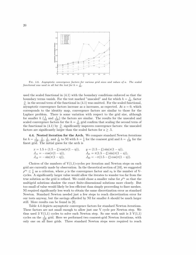
4.3. AMG tests. We next test the performance of the linear solver with varyingh. Again, the equations are linearized about the solution and the right side is set tozero. We study the deterioration in asymptotic convergence factors as a increasesfrom zero to one. The results are plotted in figure 4.6. In all but one test, we
20
0 0.1 0.2 0.3 0.4 0.5 0.6 0.7 0.8 0.9 10
0.1
0.2
0.3
0.4
0.5
0.6
0.7
a
asym
ptot
ic c
onve
rgen
ce fa
ctor
s
1/128 Grid1/64 Grid1/32 Grid1/16 Grid1/8 Grid1/4 Gridunscaled
Fig. 4.6. Asymptotic convergence factors for various grid sizes and values of a. The scaledfunctional was used in all but the test for h = 1
64.
used the scaled functional in (4.1) with the boundary conditions enforced so that theboundary terms vanish. For the test marked ”unscaled” and for which h = 1
64 , factor1
Jnin the second term of the functional in (4.1) was omitted. For the scaled functional,
asymptotic convergence factors increase as a increases, as expected. At a = 0, whichcorresponds to the identity map, convergence factors are similar to those for theLaplace problem. There is some variation with respect to the grid size, althoughfor smaller h
(164 and 1
128
)the factors are similar. The results for the unscaled and
scaled convergence factors for the h = 164 grid confirm that scaling the second term of
the functional in (4.1) by 1Jn
significantly improves convergence factors: the unscaledfactors are significantly larger than the scaled factors for a ≥ .5.
4.4. Nested iteration for the Arch. We compare standard Newton iterationsfor h = 1
128 , 164 , 1
32 , and 116 to NI with h = 1
4 for the coarsest grid and h = 1128 for the
finest grid. The initial guess for the arch is
x = 1.5 + (1.5 − ξ) cos(π(1 − η)), y = (1.5 − ξ) sin(π(1 − η)),J11 = − cos(π(1 − η)), J21 = π(1.5 − ξ) sin(π(1 − η)),J12 = − sin(π(1 − η)), J22 = −π(1.5 − ξ) cos(π(1 − η)).
Choices of the numbers of V(1,1)-cycles per iteration and Newton steps on eachgrid are currently made by observation. In the theoretical section of [10], we suggestedρν0 ≤ 1
8 as a criterion, where ρ is the convergence factor and ν0 is the number of V-cycles. A significantly larger value would allow the iterates to wander too far from thetrue solution as the grid is refined. We could chose a smaller value for ρν0 so that themultigrid solutions shadow the exact finite-dimensional solutions more closely. Buttoo small of value would likely be less efficient than simply proceeding to finer meshes.NI required significantly less work to obtain the same discretization error as standardNewton. Standard Newton needed just a few steps to reach discretization error forour tests anyway, but the savings afforded by NI for smaller h should be much largerstill. More results can be found in [9].
Table 4.4 depicts asymptotic convergence factors for standard Newton iterations.These factors are not small enough to allow just one V cycle per Newton step. Wethus used 3 V(1,1) cycles to solve each Newton step. So one work unit is 3 V(1,1)cycles on the 1
128 grid. Here we performed two coarsest-grid Newton iterations, withonly one on all finer grids. Three standard Newton steps were required to reach

21
Newton 116
132
164
1128
1 0.59 0.50 0.43 0.592 0.63 0.65 0.67 0.613 0.66 0.67 0.68 0.674 0.63 0.67 0.66 0.675 0.66 0.68 0.66 0.68
Table 4.4Asymptotic convergence factors for the V(1,1) cycle, with varying grid size and Newton itera-
tions, for the arch.
0 0.5 1 1.5 2 2.5 3 3.5 410
−2
10−1
100
101
Work Units
(Non
linea
r F
unct
iona
l) 1/2
NI1/128 Grid1/64 Grid 1/32 Grid 1/16 Grid
Fig. 4.7. Nested iteration and standard Newton for the arch.
discretization error, while NI required less than one and a half equivalents. The finalfunctional value decreases by about a factor of four as the grid size is halved, whichconfirm O(h) approximation in the H1(Ω) norm.
5. Conclusion. We showed theoretically that the nested iteration process in-volving only one discrete Newton step on each level produces a result on the finestlevel that is within discretization error of the exact solution. We also showed thisresult numerically using an H1+δ(Ω) discrete space for each of the unknowns. Futuredirections involve automating the numerical tests to include the following choices:number of relaxations before and after coarsening, number of V-cycles, number ofNewton steps on each grid, size and choice of solvers for the coarsest grid, parameter-ization of the boundary maps, and adaptive mesh refinement.
The first three choices dictate the overall efficiency of the algorithm and should beconsidered carefully for maximum effectiveness. Automation would require heuristicsto sense performance of smoothing and coarse-grid correction, as well as linearizationtrade-offs. We used one Newton step on all but the coarsest grid in our examplesand theory, but severely distorted regions may dictate more such steps to improveeffectiveness and possibly other continuation methods to address Newton’s local con-vergence characteristics. In any case, the special ability of the FOSLS functional tosignal errors could be exploited to make these choices in an effective and automaticway. The fourth coarsest-grid choice rests heavily on the geometry of the particu-lar map. Complex regions may require a fairly small coarsest grid and a significantamount of effort to solve the nonlinear problem there. Damped Newton methods andvarious forms of continuation techniques may come into play. Of course, complicated

22
regions generally require very fine meshes to supply meaningful simulations, so therelative cost of such coarsest-grid effort may again be fairly minimal. Moreover, thespecial properties of the FOSLS functional may also be exploited for these choices.The fifth choice would be to use a parameterization of the boundary in the associatedterms of the functional that would allow concentration of gird points near specialboundary features. The final choice of adaptive mesh refinement can be served bynoting that the functional value on each element is a sharp measure of the error onthat element, which makes it suitable as a measure to determine which elements needto be further subdivided (cf. [4]).
REFERENCES
[1] R.A Adams. Sobolev Spaces, volume 65 of Pure and Applied Mathematics. Academic Press,New York, 1975.
[2] S. Agmon, A. Douglis, and L. Nirenberg. Estimates near the boundary for solutions of ellipticpartial differential equations satisfying general boundary conditions II. Comm. Pure Appl.Math., 17:35–92, 1963.
[3] A.K. Aziz. The Mathematical Foundations of the Finite Element Method with Application toPartial Differential Equations. Academic Press, New York, 1972.
[4] M. Berndt, T. A. Manteuffel, and S. F. McCormick. Local error estimates and adaptive refine-ment for first-order system least-squares (FOSLS). E.T.N.A., 6:35–43, 1997.
[5] D. Braess. Finite Elements Theory, fast solvers, and applications in solid mechanics. Cam-bridge University Press, Cambridge, 1997.
[6] S.C. Brenner and L.R. Scott. The Mathematical Theory of Finite Elememt Methods, volume 15of Texts in Applied Mathematics. Springer-Verlag, New York, 1994.
[7] Z. Cai, T.A. Manteuffel, and S.F. McCormick. First-order system least squares for second-orderpartial differential equations: Part II. SIAM J. of Numer. Anal., 34:425–454, 1997.
[8] J.E. Castillo, editor. Mathematical Aspects of Numerical Grid Generation, volume 8 of Fron-tiers in Applied Mathematics. SIAM, Philadelphia, 1991.
[9] A.L. Codd. Elasticity-Fluid Coupled Systems and Elliptic Grid Generation (EGG) based onFirst-Order System Least Squares (FOSLS). PhD thesis, University of Colorado at Boul-der, 2001.
[10] A.L. Codd, T. Manteuffel, and S. McCormick. Multilevel first-order system least squares fornonlinear elliptic partial differential equations.
[11] V. Girault and P.-A. Raviart. Finite Element Methods for Navier-Stokes Equations. Springer,Berlin, 1986.
[12] P. Knupp and S. Steinberg. Fundamentals of Grid Generation. CRC Press, Boca Raton, 1993.[13] B. Lee, T. A. Manteuffel, S. F. McCormick, and J. Ruge. First-order system least-squares
(FOSLS) for the Helmholtz equation. SIAM J of Numer. Anal., 21(5):1927–1949, 2000.[14] G. Liao. On harmonic maps. In J.E. Castillo, editor, Mathematical Aspects of Numerical Grid
Generation, volume 8 of Frontiers in Applied Mathematics, chapter 9, pages 123–130.SIAM, Philadelphia, 1991.
[15] J.L. Lions and E. Magenes. Non-Homogeneous Boundary Value Problems and Applications v1, volume 181 of Die Grundlehren der mathematischen Wissenschlaften in Einzeldarstel-lungen. Springer-Verlag, Berlin, english edition, 1972.
[16] T. Rado. Aufgabe 41. Jahresbericht der Deutschen Mathematiker Vereinigung, 35:49, 1926.[17] Ja. A. Roitberg and Z.G. Seftel. A theorem on homeomorphisms for elliptic systems and its
applications. Mathematics of the USSR-Sbornik, 7(3):439–465, 1969.[18] Ya. A. Roitberg. A theorem about the complete set of isomorphisms for systems elliptic in the
sense of Douglis and Nirenberg. Ukrainian Mathematical Journal, 25(4):396–405, 1973.[19] M. Schechter. Solution of dirichlet problem for systems not necessarily strongly elliptic. Comm.
Pure Appl. Math., 12:241–247, 1959.[20] J.F. Thompson, Z.U.Z. Warsi, and C.W. Mastin. Numerical Grid Generation. North Holland,
New-York, 1985.[21] J. Wloka. Partial Differential Equations. Cambridge University Press,, Cambridge, 1987.[22] K Yosida. Functional Analysis. Springer-Verlag, Berlin, 6 edition, 1965.