Embed Size (px)
Citation preview

FACULTY OF ENGINEERING AND INFORMATION
TECHNOLOGY
Multilevel Decision Making for Supply Chain
Management
Jialin Han
A thesis submitted for the Degree of
Doctor of Philosophy
University of Technology Sydney
February, 2016

i
CERTIFICATE OF AUTHORSHIP/ORIGINALITY
This thesis is the result of a research candidature conducted jointly with another
University as part of a collaborative Doctoral degree. I certify that the work in this
thesis has not previously been submitted for a degree nor has it been submitted as part
of requirements for a degree except as part of the collaborative doctoral degree and/or
fully acknowledged within the text.
I also certify that the thesis has been written by me. Any help that I have received in
my research work and the preparation of the thesis itself has been acknowledged. In
addition, I certify that all information sources and literature used are indicated in the
thesis.
Signature of Candidate
ii
ACKNOWLEDGEMENTS
I wish to express my deep and sincere gratitude to my supervisors, Professor Jie
Lu and Professor Guangquan Zhang. It has been a great gift and pleasure to be their
student. Their comprehensive guidance has covered all aspects of my PhD study,
including research topic selection, research methodology and academic writing skills.
Their critical comments and suggestions have strengthened my study significantly.
Their respective rigorous academic skills and excellent work ethic have been an
inspiration over the course of my PhD study and I will draw upon the example they
have set throughout my future research career. Without their high order supervision
and continuous encouragement, this research could not have been completed on time.
Moreover, they have also kindly provided me with sincere help and advice when I
have sought it.
I am grateful to all members of the Decision Systems and e-Service Intelligent
(DeSI) Lab in the Center for Quantum Computation and Intelligent Systems (QCIS)
for their careful participation in my presentation and valuable comments for my
research. I would like also to thank Ms. Sue Felix and Dr. Shale Preston for helping
me to correct English presentation problems in my publications and this thesis.
I wish to express my appreciation for the financial support I received for my study.
Special thanks go to the China Scholarship Council (CSC) and the University of
Technology Sydney (UTS).
Last but not least, I would like to express my heartfelt appreciation to my family.
Thanks to my mother and father for their continuous encouragement and generous
support.
iii
ABSTRACT
Multilevel decision-making techniques aim to handle decentralized decision
problems that feature multiple decision entities distributed throughout a hierarchical
organization. Decision entities at the upper level and the lower level are respectively
termed the leader and the follower. Three challenges have appeared in the current
developments in multilevel decision-making: (1) large-scale - multilevel decision
problems become large-scale owing to high-dimensional decision variables; (2)
uncertainty - uncertain information makes related decision parameters and conditions
imprecisely or ambiguously known to decision entities; (3) diversification - multiple
decision entities that have a variety of relationships with one another may exist at
each decision level. However, existing decision models or solution approaches cannot
completely and effectively handle these large-scale, uncertain and diversified
multilevel decision problems.
To overcome these three challenges, this thesis addresses theoretical techniques
for handling three categories of unsolved multilevel decision problems and applies the
proposed techniques to deal with real-world problems in supply chain management
(SCM). First, the thesis presents a heuristics-based particle swarm optimization (PSO)
algorithm for solving large-scale nonlinear bi-level decision problems and then
extends the bi-level PSO algorithm to solve tri-level decision problems. Second,
based on a commonly used fuzzy number ranking method, the thesis develops a
compromise-based PSO algorithm for solving fuzzy nonlinear bi-level decision
problems. Third, to handle tri-level decision problems with multiple followers at the
middle and bottom levels, the thesis provides different tri-level multi-follower (TLMF)
decision models to describe various relationships between multiple followers and

iv
develops a TLMF Kth-Best algorithm; moreover, an evaluation method based on
fuzzy programming is proposed to assess the satisfaction of decision entities towards
the obtained solution. Lastly, these proposed multilevel decision-making techniques
are applied to handle decentralized production and inventory operational problems in
SCM.
v
TABLE OF CONTENTS
CERTIFICATE OF AUTHORSHIP/ORIGINALITY .................................................... i
ACKNOWLEDGEMENTS ................................................................................................... ii
ABSTRACT ..................................................................................................................... iii
TABLE OF CONTENTS ...................................................................................................... v
LIST OF FIGURES .......................................................................................................... viii
LIST OF TABLES ............................................................................................................. ix
CHAPTER 1 Introduction ............................................................................................. 1
1.1 Background ...................................................................................................... 1
1.2 Research questions and objectives ................................................................... 3
1.3 Research significance ....................................................................................... 6
1.4 Research methodology and process ................................................................. 8
1.4.1 Research methodology ........................................................................... 8
1.4.2 Research process .................................................................................. 10
1.5 Thesis structure ............................................................................................... 11
1.6 Publications related to this thesis ................................................................... 12
CHAPTER 2 Literature Review .................................................................................. 15
2.1 Bi-level decision-making ............................................................................... 15
2.1.1 Basic bi-level decision-making ............................................................ 15
2.1.2 Bi-level multi-objective decision-making ............................................ 22
2.1.3 Bi-level multi-leader and/or multi-follower decision-making ............. 23
2.2 Tri-level decision-making ............................................................................... 27
2.3 Fuzzy multilevel decision-making ................................................................. 29
2.4 Applications of multilevel decision-making techniques ................................ 31
2.4.1 Supply chain management .................................................................... 31

vi
2.4.2 Traffic and transportation network design ............................................ 34
2.4.3 Energy management ............................................................................. 37
2.4.4 Safety and accident management ......................................................... 39
2.5 Summary ........................................................................................................ 41
CHAPTER 3 Large-scale Nonlinear Multilevel Decision Making ............................. 44
3.1 Introduction .................................................................................................... 44
3.2 Bi-level PSO algorithm .................................................................................. 45
3.2.1 General bi-level decision problem and solution concepts .................... 45
3.2.2 The bi-level PSO algorithm description ............................................... 47
3.3 Tri-level PSO algorithm ................................................................................. 53
3.3.1 General tri-level decision problem and related theoretical properties . 53
3.3.2 The tri-level PSO algorithm description............................................... 57
3.4 Computational study ....................................................................................... 61
3.4.1 Small-scale benchmark problems ......................................................... 61
3.4.2 Large-scale benchmark problems ......................................................... 69
3.4.3 Assessing the efficiency performance of the bi-level PSO algorithm .. 73
3.5 Summary ........................................................................................................ 83
CHAPTER 4 Compromise-based Fuzzy Nonlinear Bi-level Decision Making ......... 85
4.1 Introduction .................................................................................................... 85
4.2 Preliminaries of fuzzy set theory .................................................................... 86
4.3 General fuzzy bi-level decision problem and theoretical properties .............. 88
4.3.1 General fuzzy Bi-level decision problem ............................................. 88
4.3.2 Related theoretical properties ............................................................... 90
4.4 Compromise-based PSO algorithm ................................................................ 93
4.5 Numerical examples ....................................................................................... 97
4.5.1 An illustrative example ......................................................................... 97
4.5.2 Benchmark examples ......................................................................... 101
4.6 Summary ...................................................................................................... 102
CHAPTER 5 Tri-level Multi-follower Decision Making .......................................... 104
vii
5.1 Introduction .................................................................................................. 104
5.2 TLMF decision models and related theoretical properties ........................... 105
5.2.1 TLMF decision models and solution concepts ................................... 106
5.2.2 Related theoretical properties ............................................................. 117
5.3 TLMF Kth-Best algorithm and a numerical example................................... 124
5.3.1 TLMF Kth-Best algorithm description ............................................... 124
5.3.2 A numerical example .......................................................................... 130
5.4 Solution evaluation ....................................................................................... 133
5.5 Case study ..................................................................................................... 139
5.5.1 Case description ................................................................................. 140
5.5.2 Model building ................................................................................... 144
5.5.3 Numerical experiment and results analysis ........................................ 146
5.5.4 Further discussions ............................................................................. 152
5.6 Summary ...................................................................................................... 154
CHAPTER 6 Application in Decentralized Vendor-managed Inventory .................. 156
6.1 Introduction .................................................................................................. 156
6.2 Problem statement ........................................................................................ 158
6.3 Analytical model ........................................................................................... 162
6.4 Computational study ..................................................................................... 165
6.4.1 An illustrative instance ....................................................................... 165
6.4.2 Sensitivity analysis ............................................................................. 169
6.4.3 Assessing the efficiency performance of the TLMF Kth-Best algorithm
..................................................................................................................... 176
6.5 Summary ...................................................................................................... 181
CHAPTER 7 Conclusions and Further Study ........................................................... 183
7.1 Conclusions .................................................................................................. 183
7.2 Further study ................................................................................................. 186
References ................................................................................................................. 188
Abbreviations ............................................................................................................ 213

viii
LIST OF FIGURES
Figure 1.1 Reasoning in the general design cycle (Vaishnavi & Kuechler Jr 2007) ..... 9
Figure 1.2 Thesis structure .......................................................................................... 12
Figure 3.1 The performance of the bi-level PSO algorithm following different
parameter combinations .............................................................................................. 78
Figure 3.2 The average of the convergent CPU time .................................................. 81
Figure 3.3 The average of the total CPU time of all iterations completed .................. 82
Figure 4.1 The membership function of fuzzy number a~ .......................................... 87
Figure 4.2 The convergence curves of the leader's and the follower's expected
objective values ......................................................................................................... 100
Figure 5.1 The organizational structure of the TLMF decision-making hierarchy ... 106
Figure 5.2 Linear membership function .................................................................... 135
Figure 5.3 Hierarchical structure of the conglomerate enterprise ............................. 141
Figure 5.4 The contrastive analysis of results ........................................................... 152
Figure 6.1 The organizational structure of the three-echelon supply chain .............. 159
Figure 6.2 The average of iterations and CPU time for solving the test problems ... 180
Figure 6.3 The fitted curve of CPU time following the number of buyers change ... 180

ix
LIST OF TABLES
Table 3.1 Benchmark problems and their related sources ........................................... 62
Table 3.2 Parameters employed in the bi-level/tri-level PSO algorithms for solving
problems 1-33 .............................................................................................................. 63
Table 3.3 The computational results for bi-level decision problems 1-25 .................. 66
Table 3.4 The computational results for tri-level decision problems 26-33 ............... 68
Table 3.5 The computational results for five-dimensional test problems 34(SMD1) -
45(SMD12) .................................................................................................................. 70
Table 3.6 The computational results for 10-dimensional test problems 46(SMD1) -
57(SMD12) .................................................................................................................. 71
Table 3.7 The computational results for 20-dimensional test problems 58-62 ........... 72
Table 3.8 Test problem dimensions ............................................................................ 74
Table 3.9 The number of test problems successfully solved under each parameter
combination ................................................................................................................. 76
Table 3.10 The computational results respectively obtained by the bi-level PSO
algorithm and GABB ................................................................................................... 79
Table 4.1 Parameters employed in the compromise-based PSO algorithm for solving
problem (4.7) ............................................................................................................... 98
Table 4.2 The computational results of problem (4.7) under different compromised
conditions .................................................................................................................... 99
Table 4.3 Parameters in the PSO algorithm for solving problems in (Zhang & Lu 2005,
2007) .......................................................................................................................... 101
Table 4.4 The computational results of the problem in (Zhang & Lu 2007) ............ 102
Table 4.5 The computational results of the problem in (Zhang & Lu 2005) ............ 102

x
Table 5.1 Notations used in the TLMF Kth-Best algorithm ...................................... 127
Table 5.2 Coefficients of model (5.3) ....................................................................... 130
Table 5.3 Objective values and corresponding satisfactory degrees of decision entities
in Example 5.1 ........................................................................................................... 138
Table 5.4 Notations for decision variables and parameters employed ...................... 143
Table 5.5 Data for the sales company ....................................................................... 146
Table 5.6 Data for the logistics centers ..................................................................... 146
Table 5.7 Data for the manufacturing factories ......................................................... 146
Table 5.8 The detailed computing process of the TLMF Kth-Best algorithm .......... 148
Table 5.9 Solutions and objective values of decision entities ................................... 149
Table 5.10 The satisfactory degree of decision entities towards solutions ............... 150
Table 6.1 Notations of decision variables and parameters employed ....................... 161
Table 6.2 Data for the vendor .................................................................................... 166
Table 6.3 Data for the distributors ............................................................................. 166
Table 6.4 Data for the buyers .................................................................................... 166
Table 6.5 The detailed computing process of the TLMF Kth-Best algorithm .......... 167
Table 6.6 Solutions and objective values of decision entities ................................... 168
Table 6.7 The experimental results based on the distributor’s and buyer's inventory
upper limits changes .................................................................................................. 171
Table 6.8 The experimental results based on the penalty cost changes .................... 173
Table 6.9 The experimental results based on the distributor’s transportation cost
changes ...................................................................................................................... 174
Table 6.10 Test instances randomly generated .......................................................... 177
Table 6.11 The experimental results of the randomly generated test problems ........ 178
PHD Thesis, UTS Chapter 1
1
CHAPTER 1 INTRODUCTION
1.1 BACKGROUND Multilevel decision-making techniques, motivated by Stackelberg game theory
(Stackelberg 1952), have been developed to address compromises between the
interactive decision entities that are distributed throughout a hierarchical organization
(Zhang, Lu & Gao 2015). In a multilevel decision-making process, decision entities at
the upper level and the lower level are respectively termed the leader and the follower
(Bard 1998), and make their individual decisions in sequence, from the leader to the
follower, with the aim of optimizing their respective objectives. This decision-making
process means that the leader has priority in making its own decision and the follower
reacts after and in full knowledge of the leader's decision; however, the leader's
decision is implicitly affected by the follower's reaction.
Bi-level decision problems and tri-level decision problems are the typical cases of
multi-level decision-making, which have motivated a number of significant efforts in
decision models, solution approaches and applications in areas of both
mathematics/computer science and business (Bard 1998; Dempe 2002; Zhang, Lu &
Gao 2015). To achieve a quick understanding of multilevel decision problems, a
tri-level decision-making case in relation to the hierarchical production-inventory
planning in a conglomerate enterprise can be taken as an example. The conglomerate
is composed of a sales company, a logistics center and a manufacturing factory, which
are distributed throughout a three-stage supply chain. To fully satisfy market demand
and shorten time-to-market, the sales company and the logistics center have to hold a
certain amount of inventory using their respective warehouses but both of them
nonetheless seek to minimize their individual inventory holding costs. When making

PHD Thesis, UTS Chapter 1
2
the production-inventory plan within a stable sales cycle, the sales company (the
leader) takes the lead in developing an optimal inventory plan which considers the
current market demand and implicit reactions of other decision entities. The logistics
center (the middle-level follower) then makes an optimal inventory plan according to
the decision given by the sales company and considers the implicit production
planning of the manufacturing factory (the bottom-level follower). Lastly, the
manufacturing factory makes the production plan to minimize its own cost of
production in light of the fixed inventory plans. The decision process will not stop
until each decision entity is unwilling to change its decision; which implies that a
compromised result or the equilibrium between the decision entities is achieved. The
example describes a typical tri-level decision problem in which decisions are
sequentially and repeatedly executed with all decision entities seeking to optimize
their individual objectives until the equilibrium between them is achieved.
Nowadays, multilevel decision problems have increasingly appeared in
decentralized management situations in the real world and have become highly
complicated, particularly with the development of economic integration and in the
current age of big data. For example, business firms usually work in a decentralized
manner in a complex supply chain network comprised of suppliers, manufacturers,
logistics companies, customers and other specialized service functions. The latest
developments of multilevel decision-making manifest three typical features: (1)
large-scale - multilevel decision problems become large-scale because of
high-dimensional decision variables; (2) uncertainty - related decision parameters and
conditions always involve uncertain information that is imprecisely or ambiguously
known to decision entities; (3) diversification - there may exist multiple decision
entities at each decision level, in which multiple decision entities at the same level
have a variety of relationships with one another.
In general, there are two fundamental issues in supporting a multilevel
decision-making process: one is how to develop a multilevel decision model to
describe such a hierarchical decision-making process, and the other is how to find an
PHD Thesis, UTS Chapter 1
3
optimal solution to the resulting decision model (Lu, Shi & Zhang 2006). However,
existing decision models or solution approaches cannot completely and effectively
handle large-scale, uncertain and diversified multilevel decision problems, which: (1)
are still time-consuming or almost impossible for solving large-scale nonlinear
bi-level and tri-level decision problems; (2) are limited to solving linear bi-level
decision problems with special uncertainty, e.g. triangular fuzzy numbers; (3) are not
applied to deal with tri-level decision problems involving multiple decision entities at
each decision level. Moreover, for the sake of handling real-world cases that appear in
highly complex decision situations, e.g. where there is uncertainty in data or multiple
decision entities are involved at each decision level, it is crucial to investigate much
more practical decision models together with solution approaches.
To support large-scale, uncertain and diversified multilevel decision-making, this
thesis addresses theoretical techniques for handling three categories of unsolved
multilevel decision problems, involving large-scale nonlinear bi-level and tri-level
decision problems, fuzzy nonlinear bi-level decision problems, and tri-level decision
problems with multiple decision entities at the middle and bottom levels; moreover,
the proposed multilevel decision-making techniques are applied to handle
decentralized management problems in supply chain management (SCM).
1.2 RESEARCH QUESTIONS AND OBJECTIVES This research aims to present practical decision models and effective solution
approaches for handling large-scale, uncertain and diversified multilevel decision
problems. The research questions are summarized as follows:
Question 1. How to solve large-scale nonlinear bi-level decision problems using an
effective algorithm and extend the algorithm to solve tri-level decision problems?
Question 2. How to solve uncertain bi-level decision problems with general fuzzy
parameters, known as fuzzy bi-level decision problems?
PHD Thesis, UTS Chapter 1
4
Question 3. How to model and solve tri-level decision problems with multiple
decision entities at the middle and bottom levels?
Question 4. How to apply the proposed multilevel decision-making techniques to
handle decentralized decision problems in applications?
This research aims to achieve the following objectives, which are expected to
answer the above research questions:
Objective 1. To develop an effective particle swarm optimization (PSO) algorithm for
solving nonlinear and large-scale bi-level decision problems. Moreover, the PSO
algorithm can be extended to solve tri-level decision problems.
This objective corresponds to research Question 1. PSO is a heuristic global
optimization algorithm first proposed by Kennedy and Eberhart (1995) which is
inspired by the social behavior of organisms such as fish schooling and bird flocking.
As PSO requires only primitive mathematical operators, and is computationally
inexpensive in terms of both memory requirements and speed (Eberhart & Kennedy
1995), it has a good convergence performance and has been successfully applied in
many fields. Multilevel decision problems have been proved to be NP-hard (Bard
1991; Ben-Aved & Blair 1990). Since traditional exact algorithmic approaches lack
universality and efficiency, this study will develop a heuristics-based PSO algorithm
for solving nonlinear and large-scale bi-level decision problems and it will extend the
bi-level PSO algorithm to solve tri-level decision problems.
Objective 2. To handle general fuzzy parameters and develop a compromise-based
PSO algorithm for solving fuzzy bi-level decision problems.
This objective corresponds to research Question 2. Fuzzy parameters involved in a
fuzzy bi-level decision problem are always characterized by fuzzy numbers (Zhang,
Lu & Gao 2015). A commonly used fuzzy number ranking method will be adopted to
handle fuzzy numbers, which can transform the fuzzy problem to a crisp problem for
ease of solving. However, the crisp problem keeps features of uncertainty, which are

PHD Thesis, UTS Chapter 1
5
determined by different understanding and identification of the leader and the
follower in relation to the uncertain decision situation. For the sake of solving the
crisp problem, the leader and the follower between themselves need to achieve a
compromised selection of uncertain decision conditions. The bi-level PSO algorithm
proposed above can be extended to solve the crisp problem.
Objective 3. To develop tri-level multi-follower (TLMF) decision models with
various relationships between multiple followers at the same level.
This objective corresponds to research Question 3. In a tri-level decision problem,
multiple decision entities are often involved at the middle and bottom levels; these
multiple decision entities are called multiple followers. Moreover, multiple followers
at the same level may have a variety of relationships with one another. For example,
followers may control their decisions independently without any information
exchange, which is called the uncooperative relationship; may make decisions
cooperatively with each other in line with the shared information, which is called the
cooperative relationship, may consider the actions of their counterparts for reference,
known as the reference-based relationship; or may be confronted with a hybrid
situation of some of the above relationships. Such diversified situations make the
decision problem complex and generate different decision processes. This category of
tri-level decision problems is known as the tri-level multi-follower (TLMF) decision
problem. This study will carefully analyze the various relationships and describe
related decision processes using different TLMF decision models.
Objective 4. To develop an effective TLMF Kth-Best algorithm for solving TLMF
decision problems and present an evaluation method to assess the solution
obtained.
This objective corresponds to research Question 3. This study will discuss
theoretical properties of TLMF decision problems in relation to the existence and
optimality of solutions. Based on related theoretical properties, a TLMF Kth-Best
algorithm will be developed. Moreover, Since the TLMF decision problem involve
PHD Thesis, UTS Chapter 1
6
multiple followers with various relationships, the solution, known as the final decision
result, cannot completely reflect the operations of the complex decision-making
process in applications. To assess the satisfaction of decision entities towards the
solution obtained, a solution evaluation method needs to be proposed.
Objective 5. To apply the proposed multilevel decision-making techniques to handle
decentralized production and inventory operational problems in SCM.
This objective corresponds to research Question 4. Driven by a new round of
industrial revolution, business firms are always distributed in a hierarchical and
networked supply chain, and it becomes very difficult for a company to be
competitive without working in close collaboration with external partners (Aguezzoul
2014). When making decisions in relation to SCM, each decision entity has to
consider decision reactions of its upstream and downstream decision entities. In this
situation, it is reasonable to apply multilevel decision-making techniques to handle
such decentralized SCM problems. This research will focus on how to model and
solve decentralized production and inventory operational problems in SCM using
multilevel decision-making techniques.
1.3 RESEARCH SIGNIFICANCE The significance of this research work can be summarized from the following
aspects.
Significance 1: the research develops a novel PSO algorithm for solving
large-scale nonlinear multilevel decision problems.
A big challenge in solving nonlinear and large-scale multilevel decision problems
is how to handle high-dimensional decision variables, nonlinear objective functions
and complex constraint conditions. In contrast to existing PSO algorithms that are
limited to solving linear or small scale bi-level decision problems, the novel PSO
algorithm is able to overcome the challenge effectively. The PSO algorithm not only
PHD Thesis, UTS Chapter 1
7
provides a practical way to solve large-scale nonlinear bi-level decision problems, but
also can be extended to solve tri-level decision problems.
Significance 2: the research develops a compromise-based PSO algorithm for
solving fuzzy nonlinear bi-level decision problems.
Within the compromise-based PSO algorithm, the leader and follower are able to
choose acceptable decision conditions based on rules of compromise due to
uncertainty, which can provide not only better solutions to benchmarks under the
specific decision situation but also different solution options due to various decision
environments. Whereas existing solution approaches are limited to handling linear
problems with special fuzzy numbers, the compromise-based PSO algorithm aims to
solve nonlinear bi-level decision problems with general fuzzy numbers.
Significance 3: the research develops theoretical techniques for handling TLMF
decision problems.
There still lack effective theoretical techniques for handling TLMF decision
problems. Accordingly, the research first proposes different TLMF decision models
that can be used to describe various relationships between multiple followers at the
same level. Second, a TLMF Kth-Best algorithm is developed to solve TLMF
decision problems, which can be also used to solve large-scale problems in reasonable
computing time. Moreover, a fuzzy programming approach is proposed to evaluate
the satisfaction of decision entities towards the solution obtained. The evaluation
method of solutions can quantitatively analyze the operation of a decision-making
process due to the changing decision environment. The above techniques provide the
theoretical foundation for TLMF decision-making research and overcomes the lack of
solution algorithms for solving TLMF decision problems.
Significance 4: the proposed multilevel decision-making techniques provide a
practical way to handle decentralized decision problems in applications.
PHD Thesis, UTS Chapter 1
8
Many decentralized decision problems have increasingly appeared in highly
complex decision situations in the real world, e.g. where there is uncertainty in data or
multiple followers are involved. The proposed multilevel decision-making techniques
can provide much more practical decision models and solution approaches for
handling these real world cases. Specifically, this research displays how to handle
decentralized production and inventory operational problems in SCM using multilevel
decision-making techniques.
1.4 RESEARCH METHODOLOGY AND PROCESS Research methodology is the “collections of problem solving methods governed
by a set of principles and a common philosophy for solving targeted problems”
(Gallupe 2007). This research belongs to the information system domain. A number
of research methodologies have been proposed and applied in the information system
domain, such as case study, field study, design research, archival research, field
experiment, laboratory experiment, survey and action research (Niu 2009; Shambour
2012; Vaishnavi & Kuechler Jr 2007).
1.4.1 RESEARCH METHODOLOGY
In this study, design research is utilized as the research methodology according to
the analysis of the research questions and objectives. Design research focuses on
crafting and analyzing artifacts in order to gain insights into research problems.
Examples of the artifacts include physical product prototypes, computer-based
information systems and human-computer interfaces. The methodology of design
research is illustrated in Figure 1.1. Generally speaking, a design research effort
includes five basic steps (Vaishnavi & Kuechler Jr 2007).

PHD Thesis, UTS Chapter 1
9
Knowledge Flows
Results
PerformanceMeasures
Artefact
Tentative Design
Proposal
Conclusion
Evaluation
Development
Suggestion
Awareness ofProblem
OutputsProcess Steps
Operation and GoalKnowledge
Circumscription
Figure 1.1 Reasoning in the general design cycle (Vaishnavi & Kuechler Jr 2007)
1) Awareness of problem
This is the starting point of a design research, at which limitations of existing
research are examined and meaningful research problems are identified. The research
problems reflect a gap between existing research and the expected status. The
awareness of problems can come from different sources: industry experience,
observations on practical applications and literature review. The corresponding output
of this step is a research proposal (Vaishnavi & Kuechler Jr 2007).
2) Suggestion
This step follows the identification of research problems, and a tentative design is
suggested. The tentative design describes what the prospective artifacts will be and
how they can be developed. Suggestion is a creative process during which new
concepts, models and approaches of artifacts are demonstrated. The resulting tentative
design of this step is usually one part of the research proposal. Thus, the output of the

PHD Thesis, UTS Chapter 1
10
suggestion step is feedback to the first step, so that the research proposal can be
revised (Vaishnavi & Kuechler Jr 2007).
3) Development
In this step, artifacts are actually built based on the suggested design. The
development of artifacts can testify to the reasonability and feasibility of the original
design and improve the original design. As a result, the development of artifacts is
often an iterative process in which an initial prototype is first built and this then
evolves when the researcher gains a deeper understanding of the research problems.
The knowledge obtained in this step is fed back to the previous two steps, which helps
researchers revise the design and the proposal (Vaishnavi & Kuechler Jr 2007).
4) Evaluation
This step considers the evaluation of the developed artifacts. The performance of
artifacts can be evaluated according to criteria defined in the research proposal and
the suggested design. The evaluation results, which might or might not meet the
expectations, are fed back to the first two steps. Thus, the proposal and design might
be revised and the artifacts might be improved (Vaishnavi & Kuechler Jr 2007).
5) Conclusion
This is the final step of a design research effort. A conclusion or end is reached as
a result of satisfaction with the evaluation results of the developed artifacts. There
might still be deviations between the suggested proposal and the artifacts that are
actually developed. However, a design research effort concludes as long as the
developed artifacts are considered as “good enough” (Vaishnavi & Kuechler Jr 2007).
1.4.2 RESEARCH PROCESS
This research was planned according to the methodology of design research. First,
a subject of multilevel decision-making was chosen as a very broad research topic of
this research. A literature review of previous research in the topic area was conducted,
PHD Thesis, UTS Chapter 1
11
and existing literature was retrieved and critically reviewed. The results of the
literature review helped to identify specific research questions to be directly addressed
in this research. As the research questions grew clearer and more definite, more
literature closely related to the research questions was reviewed. Because the existing
work in the literature lacks the ability to deal with large-scale, uncertain and
diversified multilevel decision problems, this research proposed theoretical techniques
involving decision models and solution approaches for solving such problems. The
proposed models and approaches were implemented and evaluated by numerical
experiments and/or real-world cases. According to the methodology of design
research, this research is an iterative process. As indicated in Figure 1.1, the output of
each research step might be fed back to its previous step when deviations between
expectations and evaluation results are found. Through the feedback, research
outcomes are progressively improved until satisfying results are drawn from
evaluations. Finally, writing up the PhD thesis is done at the end of the research.
1.5 THESIS STRUCTURE This thesis contains seven chapters. Chapter 1 presents the research background,
research questions, objectives, significance, research methodology and process, and
the thesis structure. Chapter 2 reviews the literature relevant to this study, including
bi-level decision-making, tri-level decision-making, fuzzy multilevel decision-making,
and the applications of multilevel decision-making techniques. Chapter 3 presents a
PSO algorithm for solving large-scale nonlinear bi-level decision problems, which
can be also extended to solve tri-level decision problems. Chapters 4 addresses related
theoretical properties of fuzzy nonlinear decision problems and develops a
compromise-based PSO algorithm. Chapter 5 proposes different TLMF decision
models to describe various relationships between multiple followers at the same level;
also, an effective solution algorithm is given. Chapter 6 applies these multilevel
decision-making techniques to handle decentralized production and inventory

PHD Thesis, UTS Chapter 1
12
operational problems in SCM. Chapter 7 provides conclusions and recommendations
for further study. The structure of the thesis is shown in Figure 1.2.
Chapter 1. Introduction
Chapter 2. Literature review
Chapter 6.Application in decentralizedvendor managed inventory
Chapter 3.Large-scale nonlinear
multilevel decisionmaking
Chapter 4.Compromise-basedfuzzy nonlinear bi-
level decision making
Chapter 7. Conclusions and FurtherStudy
Chapter 5.Tri-level multi-
follower decisionmaking
Figure 1.2 Thesis structure
1.6 PUBLICATIONS RELATED TO THIS THESIS The related papers of this thesis that are under review or published in referred
international journals and conferences are listed below.
1) Jialin Han, Jie Lu, Yaoguang Hu, Guangquan Zhang. 2015, 'Tri-level
decision-making with multiple followers: Model, algorithm and case study',
Information Sciences, vol. 311, pp. 182-204.

PHD Thesis, UTS Chapter 1
13
2) Jialin Han, Guangquan Zhang, Yaoguang Hu, Jie Lu. 2016, 'A solution to
bi/tri-level programming problems using particle swarm optimization',
Information Sciences, vol. 370-371, pp. 519-537.
3) Jialin Han, Guangquan Zhang, Jie Lu. 'Decentralized vendor-managed
inventory in a three-echelon supply chain network using tri-level
programming', European Journal of Operational Research. (Under 2nd-round
review)
4) Jialin Han, Jie Lu, Guangquan Zhang. 'Fuzzy bi-level decision model and
solution algorithm for integrated production planning and scheduling', IEEE
Transactions on Fuzzy Systems. (Under 1st-round review)
5) Jie Lu, Jialin Han, Yaoguang Hu, Guangquan Zhang. 2016, 'Multilevel
decision-making: A survey', Information Sciences, vol. 346-347, pp. 463-487.
6) Guangquan Zhang, Jialin Han, Jie Lu. 2016, 'Fuzzy bi-level decision-making:
A survey', International Journal of Computational Intelligence Systems, vol. 9,
pp. 25-34.
7) Jialin Han, Guangquan Zhang, Jie Lu, Yaoguang Hu, Shuyuan Ma. 2014,
'Model and algorithm for multi-follower tri-level hierarchical
decision-making', Lecture Notes in Computer Science, vol. 8836, pp. 398-406.
8) Jialin Han, Jie Lu, Guangquan Zhang, Yaoguang Hu. 2015, 'Solving tri-level
programming problems using a particle swarm optimization algorithm'. The
10th IEEE Conference on Industrial Electronics and Applications, pp.
569-574.
9) Jialin Han, Jie Lu, Guangquan Zhang, Yaoguang Hu. 2015, 'A
compromise-based particle swarm optimization algorithm for solving bi-level
programming problems with fuzzy parameters', The 10th International
Conference on Intelligent Systems and Knowledge Engineering, pp. 214-221.

PHD Thesis, UTS Chapter 1
14
10) Jialin Han, Jie Lu, Guangquan Zhang, Shuyuan Ma. 2014, 'Multi-follower
tri-level decision making with uncooperative followers', Decision Making and
Soft Computing: The 11th International FLINS Conference, pp. 524-529.

PHD Thesis, UTS Chapter 2
15
CHAPTER 2 LITERATURE REVIEW
This chapter reviews the research on multilevel decision-making involving
theoretical research results and applications, which are clustered into four categories:
bi-level decision-making, tri-level decision-making, fuzzy multilevel decision-making,
and applications of multilevel decision-making techniques. In Section 2.1, the bi-level
decision-making models and solution approaches are reviewed and analyzed. Section
2.2 presents the tri-level decision-making models and solution approaches. Section
2.3 addresses fuzzy multilevel (including bi-level and tri-level) decision-making
techniques. Section 2.4 discusses the applications of multilevel decision-making
techniques. A summary is given in Section 2.5.
2.1 BI-LEVEL DECISION-MAKING This section first reviews the development of techniques for solving basic bi-level
decision-making problems. It then addresses the developments of bi-level
decision-making with multiple optima involving bi-level multi-objective
decision-making, bi-level multi-leader decision-making and bi-level multi-follower
decision-making.
2.1.1 BASIC BI-LEVEL DECISION-MAKING
Basic bi-level decision-making, as found in a bi-level programming situation, has
only one decision entity attempting to optimize a unique objective at each decision
level. The general formulation for basic bi-level decision-making is described by a
bi-level program as Definition 2.1.
PHD Thesis, UTS Chapter 2
16
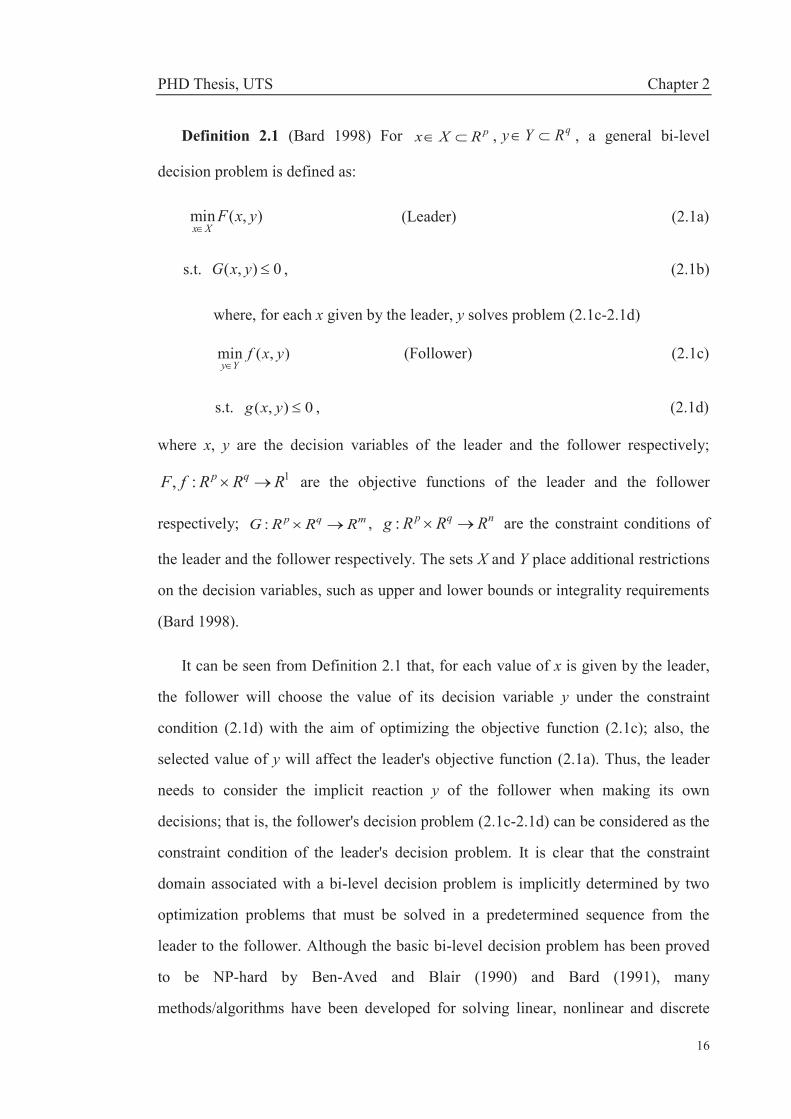
Definition 2.1 (Bard 1998) For pRXx , qRYy , a general bi-level
decision problem is defined as:
),(min yxFXx
(Leader) (2.1a)
s.t. 0),( yxG , (2.1b)
where, for each x given by the leader, y solves problem (2.1c-2.1d)
),(min yxfYy
(Follower) (2.1c)
s.t. 0),( yxg , (2.1d)
where x, y are the decision variables of the leader and the follower respectively;
1:, RRRfF qp are the objective functions of the leader and the follower
respectively; mqp RRRG : , nqp RRRg : are the constraint conditions of
the leader and the follower respectively. The sets X and Y place additional restrictions
on the decision variables, such as upper and lower bounds or integrality requirements
(Bard 1998).
It can be seen from Definition 2.1 that, for each value of x is given by the leader,
the follower will choose the value of its decision variable y under the constraint
condition (2.1d) with the aim of optimizing the objective function (2.1c); also, the
selected value of y will affect the leader's objective function (2.1a). Thus, the leader
needs to consider the implicit reaction y of the follower when making its own
decisions; that is, the follower's decision problem (2.1c-2.1d) can be considered as the
constraint condition of the leader's decision problem. It is clear that the constraint
domain associated with a bi-level decision problem is implicitly determined by two
optimization problems that must be solved in a predetermined sequence from the
leader to the follower. Although the basic bi-level decision problem has been proved
to be NP-hard by Ben-Aved and Blair (1990) and Bard (1991), many
methods/algorithms have been developed for solving linear, nonlinear and discrete

PHD Thesis, UTS Chapter 2
17
bi-level decision problems. This section reviews the research of these three categories
of basic bi-level decision-making techniques.
2.1.1.1 LINEAR BI-LEVEL DECISION-MAKING
Definition 2.2 (Bard 1998) Based on Definition 2.1, for pRXx ,
qRYy , and 1:, RRRfF qp , the linear bi-level decision problem can be
written as follows:
ydxcyxFXx 11),(min (Leader) (2.2a)
s.t. 111 byBxA , (2.2b)
where, for each x given by the leader, y solves problem (2.2c-2.2d)
ydxcyxfYy 22),(min (Follower) (2.2c)
s.t. 222 byBxA , (2.2d)
where pRcc 21, , qRdd 21, , mRb1 , nRb2 , pmRA1 , qmRB1 ,
pnRA2 , qnRB2 .
In terms of solving linear bi-level decision problems, the traditional algorithms
can be classified into three main categories: the vertex enumeration approaches
(Bialas & Karwan 1984; Candler & Townsley 1982; Shi, Lu & Zhang 2005; Tuy,
Migdalas & Värbrand 1993) based on an important characteristic of bi-level
programming whereby an optimal solution occurs at a vertex of the constraint region;
the Kuhn-Tucker approaches involving branch and bound algorithms (Bard & Falk
1982; Bard & Moore 1990; Fortuny-Amat & McCarl 1981; Shi et al. 2006) and
complementary pivot algorithms (Bialas & Karwan 1984; Júdice & Faustino 1992;
Önal 1993), in which the upper-level problem includes the lower-level’s optimality
conditions as extra constraints; and the penalty function approaches (Anandalingam &
PHD Thesis, UTS Chapter 2
18
White 1990; White & Anandalingam 1993) which append a penalty term of the
lower-level problem to the objective function of the upper-level problem.
In recent years, Audet, Haddad and Savard (2007) proposed a disjunctive cuts
method for a linear bi-level decision problem with continuous variables. Audet,
Savard and Zghal (2007) considered the equivalences between linear mixed 0-1
integer programming problems and linear bi-level decision problems, and proposed a
finite and exact branch-and-cut algorithm for solving such problems. Glackin, Ecker
and Kupferschmid (2009) addressed the relationship between linear multi-objective
programs and linear bi-level programs and presented an algorithm for solving linear
bi-level programs that uses simplex pivots on an expanded tableau. Calvete and Galé
(2012) addressed linear bi-level programs in which the coefficients of both objective
functions are interval numbers and developed two algorithms based on ranking
extreme points to solve such problems. Ren and Wang (2014) proposed a cutting
plane method to solve the linear bi-level decision problem with interval coefficients in
both objective functions.
A range of heuristic algorithms have been also developed to solve bi-level
decision problems. Gendreau, Marcotte and Savard (1996) used an adaptive search
method related to the tabu search meta-heuristic to solve the linear bi-level decision
problem. Hejazi et al. (2002) proposed a method based on genetic algorithm for
solving linear bi-level decision problems. Lan et al. (2007) proposed a hybrid
algorithm that combines neural network and tabu search for solving linear bi-level
decision problems. Calvete, Galee and Mateo (2008) developed a genetic algorithm
for solving a class of linear bi-level decision problems in which both objective
functions are linear and the common constraint region is a polyhedron; the authors
also presented a method for the test set construction of linear bi-level decision
problems especially for generating large-scale problems, which can be employed to
assess the efficiency performance of related algorithms. Kuo and Huang (2009)
developed a particle swarm optimization (PSO) algorithm with swarm intelligence to
PHD Thesis, UTS Chapter 2
19
solve linear bi-level decision problems. Hu et al. (2010) presented a neural network
approach for solving linear bi-level decision problems.
2.1.1.2 NONLINEAR BI-LEVEL DECISION-MAKING
With respect to Definition 2.1, if the objective functions ),( yxF , ),( yxf or the
constraint conditions 0),( yxG , 0),( yxg are nonlinear formulations, the
bi-level program is known as a nonlinear bi-level decision problem, which is much
more difficult to solve than linear versions.
In early research in solving nonlinear bi-level decision problems, Bard (1988)
extended the traditional branch and bound algorithm to solve nonlinear convex
bi-level decision problems. Edmunds and Bard (1991) used a branch-and-bound
algorithm and a cutting-plane algorithm to solve various versions of nonlinear bi-level
decision problems when certain convexity conditions hold. Al-Khayyal, Horst and
Pardalos (1992) developed a branch and bound algorithm and a piecewise linear
approximation method to find the global minimum for a class of nonlinear bi-level
decision problems based on an equivalent system of convex and separable quadratic
constraints. Vicente and Calamai (1994) introduced two descent methods for a special
instance of bi-level programs where the second-level problem is strictly convex
quadratic.
In recent years, Tuy, Migdalas and Hoai-Phuong (2007) showed that a nonlinear
bi-level decision problem can be transformed into a monotonic optimization problem
which can then be solved by a branch-reduce-and-bound method using monotonicity
cuts. Mitsos, Lemonidis and Barton (2008) presented a bounding algorithm for the
global solution of nonlinear bi-level programs involving nonconvex objective
functions in both decision levels. Mersha and Dempe (2011) studied the application of
a class of direct search methods and solved bi-level decision problems containing
convex lower level problems with strongly stable optimal solutions.

PHD Thesis, UTS Chapter 2
20
In regard to related heuristic algorithms, Wang, Jiao and Li (2005) transformed a
special nonlinear bi-level decision problem into an equivalent single objective
nonlinear programming problem that can be solved by an evolutionary algorithm.
Wan, Wang and Sun (2013) presented a hybrid intelligent algorithm of PSO and
chaos searching technique for solving nonlinear bi-level decision problems. Wan,
Mao and Wang (2014) also developed a novel evolutionary algorithm, called the
estimation of distribution algorithm, for solving a special class of nonlinear bi-level
decision problems in which the lower-level problem is a convex program for each
given upper-level decision. Lv et al. (2008), Lv, Chen and Wan (2010) and He et al.
(2014) proposed neural network methods for solving nonlinear bi-level decision
problems. It is notable that Sinha, Malo and Deb (2014) proposed a procedure for
designing the test set of nonlinear bi-level decision problems and presented the
corresponding computational results for these test problems using a nested bi-level
evolutionary algorithm. Researchers can consider these test problems as the
benchmark for examining the effectiveness of their own algorithms.
2.1.1.3 DISCRETE BI-LEVEL DECISION-MAKING
In many bi-level decision-making problems, a subset of the variables is restricted
to take on discrete values (Bard 1998). A problem can be considered to be a general
discrete bi-level decision problem when the decision variables in Definition 2.1 are
discrete, e.g. integer programming. Clearly, if the decision variables are discrete
rather than continuous, the linear bi-level decision problem (2.2) will become a
discrete linear bi-level program.
Discrete variables can complicate bi-level decision problems by several orders of
magnitude and render all but the smallest instances unsolvable (Bard 1998). Wen and
Yang (1990), Moore and Bard (1990), and Bard and Moore (1992) therefore proposed
traditional branch and bound algorithms for finding solutions to integer linear bi-level
decision-making problems. Edmunds and Bard (1992) developed a branch and bound
algorithm to solve a mixed-integer nonlinear bi-level decision problem. Vicente,

PHD Thesis, UTS Chapter 2
21
Savard and Judice (1996) designed penalty function methods for solving discrete
linear bi-level decision problems.
Recently, Faísca, Dua, et al. (2007) proposed a global optimization approach to
solve quadratic bi-level and mixed integer linear bi-level problems, with or without
right-hand-side uncertainty. Mitsos (2010) presented an algorithm based on the
research by Mitsos, Lemonidis and Barton (2008) for the global optimization of
nonlinear bi-level mixed-integer programs, which relies on a convergent lower bound
and an optional upper bound. Köppe, Queyranne and Ryan (2010) proposed a
parametric integer programming algorithm for solving a mixed integer linear bi-level
decision problem where the follower solves an integer program with a fixed number
of variables. Domínguez and Pistikopoulos (2010) addressed two algorithms using
multiparametric programming techniques respectively for solving two categories of
integer bi-level decision problems: one category consists of pure integer problems
where integer variables of the first level appear in the linear or polynomial problem of
the second level, and the other consists of mixed-integer problems where integer and
continuous variables of the first level appear in the linear or polynomial problem of
the second level. Xu and Wang (2014) solved a mixed integer linear bi-level decision
problem using an exact algorithm. The algorithm relies on three simplifying
assumptions, explicitly considers finite optimal, infeasible and unbounded cases, and
is proved to terminate finitely and correctly. Sharma, Dahiya and Verma (2014)
discussed an integer bi-level decision problem with bounded variables in which the
objective function of the first level is linear fractional, the objective function of the
second level is linear and the common constraint region is a polyhedron. They
proposed an iterative algorithm to find an optimal solution to the problem.
In relation to heuristic algorithms for solving discrete bi-level decision problems,
Wen and Huang (1996) reported a mixed-integer linear bi-level decision-making
formulation in which zero-one decision variables are controlled by the first level and
real-value decision variables are controlled by the second level. An algorithm based
on the short term memory component of tabu search, called simple tabu search, was
PHD Thesis, UTS Chapter 2
22
developed to solve the problem. Nishizaki and Sakawa (2005) presented a method
using genetic algorithms for obtaining optimal solutions to integer bi-level decision
problems.
2.1.2 BI-LEVEL MULTI-OBJECTIVE DECISION-MAKING
When multiple conflicting objectives for each decision entity exist in a bi-level
decision problem, this is known as a bi-level multi-objective (BLMO) decision
problem.
Definition 2.3 (Deb & Sinha 2010) For pRXx , qRYy , a general
BLMO decision problem is formulated as:
)),(,),,(),,((),(min 21 yxFyxFyxFyxF MXx (Leader) (2.3a)
s.t. 0),( yxG , (2.3b)
where, for each x given by the leader, y solves problem (2.3c-2.3d)
)),(,),,(),,((),(min 21 yxfyxfyxfyxf NYy (Follower) (2.3c)
s.t. 0),( yxg , (2.3d)
where x, y are the decision variables of the leader and the follower respectively;
1:, RRRfF qpji , Mi ,,2,1 , Nj ,,2,1 are the conflicting objective
functions of the leader and the follower respectively; mqp RRRG : ,
nqp RRRg : are the constraint conditions of the leader and the follower
respectively. The sets X and Y place additional restrictions on the decision variables,
such as upper and lower bounds or integrality requirements.
Many algorithms have been developed to solve bi-level multi-objective (BLMO)
decision problems in various versions. Ankhili and Mansouri (2009) addressed a class
of linear bi-level programs where the upper level is a linear scalar optimization
problem and the lower level is a linear multi-objective optimization problem; they
PHD Thesis, UTS Chapter 2
23
approached the problems via an exact penalty method. Calvete and Galé (2010)
presented a number of methods of computing efficient solutions to solve linear
bi-level decision problems with multiple objectives at the upper level; all the methods
result in solving linear bi-level problems with a single objective function at each level
based on both weighted sum scalarization and scalarization techniques. Eichfelder
(2010) discussed a nonlinear nonconvex BLMO decision problem using an optimistic
approach in which the feasible points of the upper-level objective function can be
expressed as the set of minimal solutions of a single-level multi-objective
optimization problem. The BLMO decision problem is then solved by an iterative
process, again using sensitivity theorems. Emam (2013) proposed an interactive
approach for solving bi-level integer fractional multi-objective decision problems.
From the aspect of using heuristic algorithms for solving BLMO decision
problems, Deb and Sinha (2010) proposed a viable and hybrid
evolutionary-cum-local-search based algorithm for solving BLMO decision problems.
Note that Deb and Sinha (2009) also presented a method for constructing the test set
of BLMO decision problems. Calvete and Galé (2011) developed an exact algorithm
and a metaheuristic algorithm to solve linear bi-level decision problems with multiple
objectives at the lower level. Zhang et al. (2013) proposed a hybrid PSO algorithm
with crossover operator to solve high dimensional bi-level multi-objective decision
problems. Alves and Costa (2014) presented an improved PSO algorithm to solve
linear bi-level decision problems with multiple objectives at the upper level.
2.1.3 BI-LEVEL MULTI-LEADER AND/OR
MULTI-FOLLOWER DECISION-MAKING
In a bi-level decision problem, multiple decision entities may exist at each level,
and this is known as a bi-level multi-leader and/or multi-follower decision problem. A
general bi-level multi-leader (BLML) decision problem can be defined as Definition
2.4.
PHD Thesis, UTS Chapter 2
24
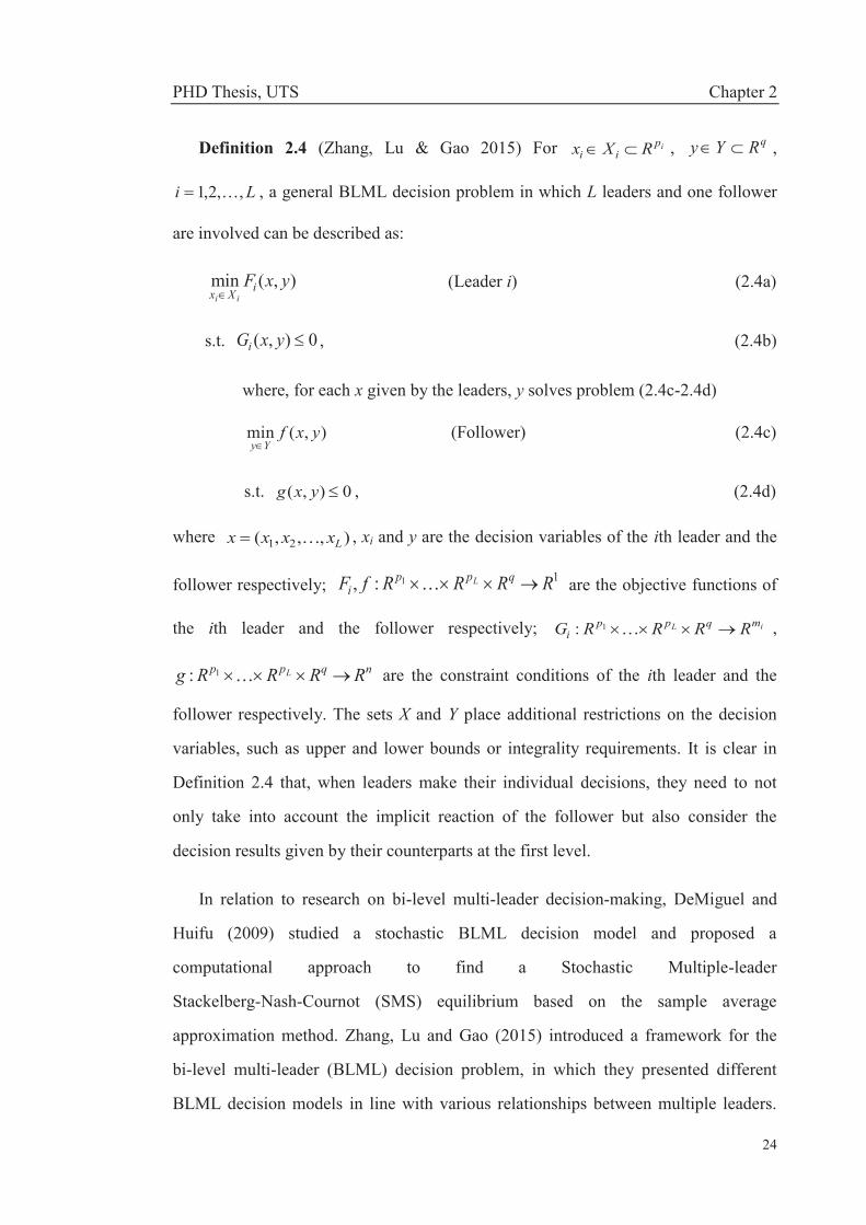
Definition 2.4 (Zhang, Lu & Gao 2015) For ipii RXx , qRYy ,
Li ,,2,1 , a general BLML decision problem in which L leaders and one follower
are involved can be described as:
),(min yxFiXx ii (Leader i) (2.4a)
s.t. 0),( yxGi , (2.4b)
where, for each x given by the leaders, y solves problem (2.4c-2.4d)
),(min yxfYy
(Follower) (2.4c)
s.t. 0),( yxg , (2.4d)
where ),,,( 21 Lxxxx , xi and y are the decision variables of the ith leader and the
follower respectively; 11:, RRRRfF qppi
L are the objective functions of
the ith leader and the follower respectively; iL mqppi RRRRG 1: ,
nqpp RRRRg L1: are the constraint conditions of the ith leader and the
follower respectively. The sets X and Y place additional restrictions on the decision
variables, such as upper and lower bounds or integrality requirements. It is clear in
Definition 2.4 that, when leaders make their individual decisions, they need to not
only take into account the implicit reaction of the follower but also consider the
decision results given by their counterparts at the first level.
In relation to research on bi-level multi-leader decision-making, DeMiguel and
Huifu (2009) studied a stochastic BLML decision model and proposed a
computational approach to find a Stochastic Multiple-leader
Stackelberg-Nash-Cournot (SMS) equilibrium based on the sample average
approximation method. Zhang, Lu and Gao (2015) introduced a framework for the
bi-level multi-leader (BLML) decision problem, in which they presented different
BLML decision models in line with various relationships between multiple leaders.
PHD Thesis, UTS Chapter 2
25
The authors also proposed a PSO algorithm to find a solution for BLML decision
problems based on the related solution concepts.
In contrast to the limited discussion on BLML decision-making, researchers have
paid considerably more attention to bi-level multi-follower (BLMF) decision-making.
A general BLMF decision problem in which one leader and k followers are involved
can be defined as Definition 2.5.
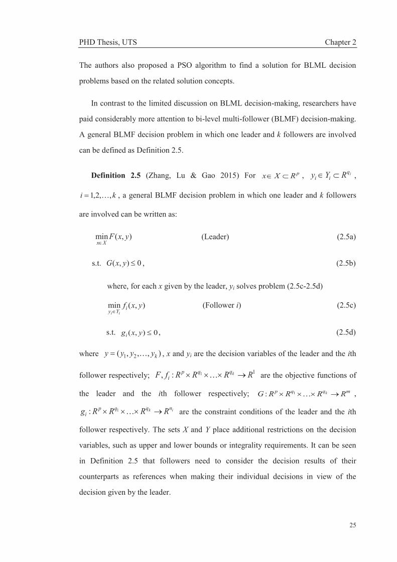
Definition 2.5 (Zhang, Lu & Gao 2015) For pRXx , iqii RYy ,
ki ,,2,1 , a general BLMF decision problem in which one leader and k followers
are involved can be written as:
),(min yxFXx
(Leader) (2.5a)
s.t. 0),( yxG , (2.5b)
where, for each x given by the leader, yi solves problem (2.5c-2.5d)
),(min yxfiYy ii
(Follower i) (2.5c)
s.t. 0),( yxgi , (2.5d)
where ),,,( 21 kyyyy , x and yi are the decision variables of the leader and the ith
follower respectively; 11:, RRRRfF kqqpi are the objective functions of
the leader and the ith follower respectively; mqqp RRRRG k1: ,
ik nqqpi RRRRg 1: are the constraint conditions of the leader and the ith
follower respectively. The sets X and Y place additional restrictions on the decision
variables, such as upper and lower bounds or integrality requirements. It can be seen
in Definition 2.5 that followers need to consider the decision results of their
counterparts as references when making their individual decisions in view of the
decision given by the leader.
PHD Thesis, UTS Chapter 2
26
Anandalingam and Apprey (1991) first presented a linear BLMF decision model,
known as a linear bi-level multi-agent system, and developed a penalty function
approach to solve the problem. Liu (1998) designed a genetic algorithm for solving
Stackelberg-Nash equilibrium of nonlinear BLMF decision problems in which there
might be an information exchange between the followers. Based on previous research,
Lu, Shi and Zhang (2006) proposed a general framework of BLMF decision-making
that considers three main relationships between multiple followers: the uncooperative
relationship, the referential-uncooperative relationship, and the partial-cooperative
relationship. The research on BLMF decision-making after Lu, Shi and Zhang (2006)
was structured on the general framework. Calvete and Galé (2007) subsequently
presented a approach for solving the linear BLMF decision problem with
uncooperative followers, which converted the BLMF problem to a bi-level problem
with one leader and one follower. Shi, Zhang and Lu (2005) and Shi et al. (2007)
extended the Kth-Best algorithm to solve linear BLMF decision problems with
uncooperative and partial-cooperative relationships respectively between followers.
Lu et al. (2007) and Lu and Shi (2007) respectively adopted the extended
Kuhn-Tucker algorithm and the extended branch and bound algorithm to solve the
referential-uncooperative linear BLMF decision problem.
Nie (2011) developed and characterized discrete-time dynamic bi-level
multi-leader and multi-follower (BLMLMF) games with leaders in turn, and a
dynamic programming algorithm was employed to solve this problem. Gao (2010)
developed PSO-based algorithms to solve BLML, BLMF and BLMLMF decision
problems. Sinha et al. (2014) used a computationally intensive nested evolutionary
algorithm to find an optimal solution for a multi-period BLMLMF decision problem
with nonlinear and discrete variables.

PHD Thesis, UTS Chapter 2
27
2.2 TRI-LEVEL DECISION-MAKING Decentralized decision-making problems within a hierarchical system are often
comprised of more than two levels in many applications, which is known as tri-level
and multilevel decision-making.
Definition 2.6 (Faísca, Saraiva, et al. 2007) For pRXx , qRYy ,
rRZz , a general tri-level decision problem is defined as:
),,(min 1 zyxfXx
(Leader) (2.6a)
s.t. 0),,(1 zyxg , (2.6b)
where, for each x given by the leader, (y, z) solves the problems (2.6c-2.6f)
of the middle-level and bottom-level followers:
),,(min 2 zyxfYy
(Middle-level follower) (2.6c)
s.t. 0),,(2 zyxg , (2.6d)
where, for each (x, y) given by the leader and the middle-level follower,
z solves the problem (2.6e-2.6f) of the bottom-level follower:
),,(min 3 zyxfZz
(Bottom-level follower) (2.6c)
s.t. 0),,(3 zyxg , (2.6d)
where x, y, z are the decision variables of the leader, the middle-level follower and the
bottom-level follower respectively; 1321 :,, RRRRfff rqp are the objective
functions of the three decision entities respectively; 3,2,1,: iRRRRg ikrqpi
are the constraint conditions of the three decision entities respectively.
While the majority of studies on multilevel decision-making have focused on
bi-level decision-making, research on tri-level decision problems has increasingly

PHD Thesis, UTS Chapter 2
28
attracted investigations into solution approaches since tri-level decision-making can
be applied to handle many decentralized decision problems in the real world (Lu et al.
2012). Bard (1984) first presented an investigation into linear tri-level
decision-making and designed a cutting plane algorithm to solve such problems,
based on which White (1997) proposed a penalty function approach for linear tri-level
decision problems. Anandalingam (1988) and Sinha (2001) developed Kuhn-Tucker
transformation methods to find local optimal solutions for linear tri-level decision
problems. Ruan et al. (2004) discussed the optimality conditions and related
geometric properties of a linear tri-level decision problem with dominated objective
functions. Faísca, Saraiva, et al. (2007) studied a multi-parametric programming
approach to solve tri-level hierarchical and decentralized optimization problems based
on parametric global optimization for bi-level decision-making (Faísca, Dua, et al.
2007). Zhang et al. (2010) developed a tri-level Kth-Best algorithm to solve linear
tri-level decision problems.
A category of approaches based on fuzzy programming has been also developed
to solve multilevel decision problems involving bi-level and tri-level programs. Lai
(1996) first proposed a fuzzy approach to find a satisfactory solution to the linear
multilevel decision problem using concepts of membership functions of individual
optimality and the satisfactory degree of individual decision power. Shih, Lai and Lee
(1996) extended Lai’s concepts and adopted tolerance membership functions and
multiple objective optimization to develop a fuzzy approach for solving the above
problems. Sakawa, Nishizaki and Uemura (1998) presented an interactive fuzzy
programming approach for linear multilevel decision problems by updating the
satisfactory degrees of decision entities at the upper level with considerations of
overall satisfactory balance between all levels. Their interactive fuzzy programming
approach overcomes the inconsistency between the fuzzy goals of objectives and
decision variables that existed in the research developed by Lai (1996) and Shih, Lai
and Lee (1996). Sinha (2003a, 2003b) developed an alternative multilevel decision
technique based on fuzzy mathematical programming, which considered a sequential

PHD Thesis, UTS Chapter 2
29
order of the multilevel hierarchy and took into account the preference of the decision
entity at each level. Pramanik and Roy (2007) and Arora and Gupta (2009) each
proposed a fuzzy goal programming approach to solve linear multilevel decision
problems using definitions of tolerance membership functions and satisfactory degree
of decision entities.
To solve tri-level decision-making problems with multiple optima, Shih, Lai and
Lee (1996) proposed a tri-level decision model with multiple followers and developed
a fuzzy approach to solve the model. Lu et al. (2012) presented a framework for
tri-level multi-follower (TLMF) decision-making research and discussed various
relationships between multiple followers.
2.3 FUZZY MULTILEVEL DECISION-MAKING A multilevel decision problem in which the parameters are described by fuzzy
values, often characterized by fuzzy numbers, is called a fuzzy multilevel decision
problem (Zhang & Lu 2007; Zhang, Lu & Gao 2015). For the sake of simplicity, this
section presents a general fuzzy linear bi-level decision problem based on Definition
2.2, described as Definition 2.7.
Definition 2.7 (Zhang & Lu 2005; Zhang, Lu & Gao 2015) For pRXx ,
qRYy , and )(:, RFRRfF qp , a general fuzzy linear bi-level decision
problem can be written as follows:
ydxcyxFXx 11
~~),(min (Leader) (2.7a)
s.t. 111~~~ byBxA , (2.7b)
where, for each x given by the leader, y solves problem (2.7c-2.7d)
ydxcyxfYy 22
~~),(min (Follower) (2.7c)
s.t. 222~~~ byBxA , (2.7d)

PHD Thesis, UTS Chapter 2
30
where )(~,~21 RFcc p , )(~,~
21 RFdd q , )(~1 RFb m , )(~
2 RFb n , )(~1 RFA pm ,
)(~1 RFB qm , )(~
2 RFA pn , )(~2 RFB qn , F(R) is the set of all finite fuzzy
numbers.
Like multilevel decision-making under certainty, the majority of the research on
fuzzy multilevel decision-making has focused on bi-level versions that have
motivated numerous solution approaches (Zhang, Lu & Gao 2015). Zhang and Lu
(2005) proposed a general fuzzy linear bi-level decision problem and developed an
approximation Kuhn-Tucker approach to solve this problem. They also presented an
approximation Kth-Best algorithm to solve the fuzzy linear bi-level decision problem
(Zhang & Lu 2007). Gao et al. (2008) proposed a programmable λ-cut approximation
algorithm to solve a λ-cut set based fuzzy goal bi-level decision problem. Budnitzki
(2013) used the selection function approach and a modified version of the Kth-Best
algorithm to solve a fuzzy linear bi-level decision problem. Sakawa, Nishizaki and
Uemura (2000a) proposed an interactive fuzzy programming approach to find a
satisfactory solution to a fuzzy linear bi-level decision problem. Pramanik (2012)
adopted a fuzzy goal programming approach to solve fuzzy linear bi-level decision
problems.
Fuzzy bi-level decision-making with multiple optima has attracted numerous
studies. Zhang, Lu and Dillon (2007a) developed an approximation branch-and-bound
algorithm to solve a fuzzy linear BLMO decision problem. Gao et al. (2010) proposed
a λ-cut and goal-programming-based algorithm to solve fuzzy linear BLMO decision
problems. Gao, Zhang and Lu (2009) focused on the fuzzy linear bi-level decision
problem with multiple followers who share the common constraints and developed a
PSO algorithm to solve the problem. Gao and Liu (2005) integrated fuzzy simulation,
neural network and genetic algorithm to produce a hybrid intelligent algorithm for
solving a fuzzy nonlinear bi-level decision problem with multiple followers. Zhang,
Lu and Dillon (2007b) proposed a set of fuzzy linear bi-level multi-objective
multi-follower (BLMOMF) decision models and developed an extended branch and
PHD Thesis, UTS Chapter 2
31
bound algorithm to solve such problems. Zhang and Lu (2010) developed an
approximation Kth-Best algorithm to solve fuzzy linear BLMOMF decision problems
with a cooperative relationship among multiple followers. Zhang, Lu and Gao (2008)
developed an approximation branch-and-bound algorithm to solve a fuzzy linear
BLMOMF decision problem with a partial cooperative relationship among multiple
followers.
In terms of the discussion about fuzzy tri-level and multilevel decision-making,
Sakawa, Nishizaki and Uemura (2000a) extended their bi-level interactive fuzzy
programming approach to solve fuzzy linear multilevel decision problems. They also
extended the fuzzy approach to solve fuzzy linear multilevel fractional decision
problems (Sakawa, Nishizaki & Uemura 2000b), fuzzy multilevel 0-1 decision
problems (Sakawa, Nishizaki & Hitaka 2001) and fuzzy multilevel non-convex
decision problems (Sakawa & Nishizaki 2002). Based on interactive fuzzy
programming approaches, Osman et al. (2004) studied a fuzzy non-linear tri-level
decision problem with multiple objectives.
2.4 APPLICATIONS OF MULTILEVEL
DECISION-MAKING TECHNIQUES Multilevel decision-making techniques have been widely applied to handle
decentralized decision problems in the real world, in particular in the last five years.
These applications largely fall into the following four areas: (1) supply chain
management; (2) traffic and transportation network design; (3) energy management;
and (4) safety and accident management.
2.4.1 SUPPLY CHAIN MANAGEMENT
Supply chain management (SCM) requires decentralized decisions to be made at
several stages in a complex hierarchical system which includes the location of
business firms, the acquisition of raw materials, production planning and operations,
PHD Thesis, UTS Chapter 2
32
inventory control, and the delivery and pricing of commodities. It is increasingly
important to develop an efficient and easily-applicable decision-making methodology
to handle conflict coordination and the decentralized nature of SCM (Li & Cruz Jr
2009; Sana 2011). In recognition of this, multilevel decision-making techniques have
been applied to deal with many of the decentralized decision-making problems found
in SCM.
Multilevel decision-making techniques in SCM have largely been applied to deal
with the competitive location of facilities, production planning and operations,
commodities distribution and pricing. With respect to the competitive location of
facilities in SCM, Plastria and Vanhaverbeke (2008) used bi-level programs to adapt
the competitive location model based on maximal covering to include the knowledge
that a competitor will eventually enter the market with a single new facility.
Küçükaydin, Aras and Kuban Altınel (2011) studied a problem in which a firm or
franchise enters a market by locating new facilities near existing facilities belonging
to a competitor and formulated the problem as a mixed-integer nonlinear bi-level
decision model in which the firm entering the market is the leader and the competitor
is the follower. Rider et al. (2013) presented a bi-level decision model for determining
optimal location and contract pricing of distributed generation in radial distribution
systems where the upper-level optimization determines the allocation and contract
prices of the distributed generation units, whereas the lower-level optimization
models the reaction of the distribution company. Gang et al. (2015) proposed a
bi-level multi-objective optimization model for a stone industrial park location
problem with a hierarchical structure consisting of a local government and several
stone enterprises in a random environment. The problem was solved using a bi-level
interactive method based on a satisfactory solution and adaptive chaotic PSO.
For decentralized production planning and operations, Lukač, Šorić and
Rosenzweig (2008) designed a mixed 0-1 integer bi-level decision model for a
production planning problem with sequence dependent setups, in which the objective
of the leader is to assign the products to the machines in order to minimize the total

PHD Thesis, UTS Chapter 2
33
sequence dependent setup time, while the objective of the follower is to minimize the
production, storage and setup cost of the machine. They developed a heuristic
algorithm based on tabu search to solve the problem. Calvete, Galé and Oliveros
(2011) proposed a bi-level program to model a hierarchical production-distribution
planning problem in which two decision makers respectively controlling the
production process and the distribution process do not cooperate because of different
optimization strategies. An ant colony optimization approach was developed to solve
the bi-level model. Kasemset and Kachitvichyanukul (2012) presented a bi-level
multi-objective mathematical model for a TOC (theory of constraints)-based job-shop
scheduling problem and developed a PSO algorithm to solve the problem.
In terms of using multilevel decision-making techniques to handle commodities
distribution and pricing problems in SCM, Gao et al. (2011) established two bi-level
pricing models for pricing problems between the vendor and the buyer, designated as
the leader and the follower respectively, in a two-echelon supply chain. They
developed a PSO-based algorithm to solve problems defined by these bi-level pricing
models. Kuo and Han (2011) applied linear bi-level programming to model a supply
chain distribution problem and developed an efficient method based on a hybrid of the
genetic algorithm and PSO algorithm to solve the resulting decision model. Kis and
Kovács (2013) studied an extension of the classical uncapacitated lot-sizing problem
with backlogs, in which two autonomous and self-interested decision makers
constitute a two-echelon supply chain. Qiu and Huang (2013) presented a bi-level
decision model and an enumerative algorithm to describe and solve a SCM problem
in which a supply hub in an industrial park and manufacturers interact to make their
decisions on pricing, replenishment and delivery. Calvete, Galé and Iranzo (2014)
addressed a mixed integer bi-level optimization model for the planning of a
decentralized distribution network consisting of manufacturing plants, depots and
customers, and a metaheuristic approach based on evolutionary algorithms was
developed to solve the optimization model. Ma, Wang and Zhu (2014) considered a
two-echelon supply chain system with one manufacturer and one retailer, in which the
PHD Thesis, UTS Chapter 2
34
manufacturer first purchases raw materials from the supplier; following production
and processing by the manufacturer, the end products are sold to the retailer. By
switching the leader and follower roles between the manufacturer and the retailer, the
authors established two bi-level decision models for joint pricing and lot-sizing and
developed a PSO algorithm to solve the resulting models.
A number of researchers have applied multilevel decision-making techniques to
handle product design, raw materials supply and inventory control problems in SCM.
Yang et al. (2015) formulated a mixed 0-1 nonlinear bi-level decision model for the
joint optimization of product family configuration and scaling design, in which a
bi-level decision structure reveals coupled decision making between module
configuration and parameter scaling. Based on a conditional value-at-risk (CVaR)
measure of risk management, Xu, Meng and Shen (2013) proposed a tri-level decision
model for the three-echelon SCM in which the material supplier and the manufacturer
maximize their own profit while the retailer maximizes its CVaR of the expected
profit. The authors showed that the proposed tri-level decision model can be
transformed into a bi-level decision model that can be solved by existing methods.
2.4.2 TRAFFIC AND TRANSPORTATION NETWORK
DESIGN
Severe traffic and transportation delays are incurred in most road networks as a
result of continuously growing travel demand, increasing traffic congestion,
transportation allocation problems between supply and demand nodes, and optimal
transportation route problems. The rapid growth of overload in traffic and
transportation networks has motivated decision makers to apply multilevel
decision-making techniques to cope with the related decision-making and
optimization problems in decentralized situations.
Extensive research on the basis of multilevel decision-making has been devoted to
road network design problems as a result of insufficient provision of link capacity for

PHD Thesis, UTS Chapter 2
35
travel demand surges. Cao et al. (2007) used a discrete bi-level decision model to
describe the relationship of the benefit-cost of the traffic flow guidance system (TFGS)
and the equilibrium of users, and presented an arithmetic based on sensitivity analysis.
In a system which allows buses of different sizes to be assigned to public transport
routes, dell’Olio, Ibeas and Ruisánchez (2012) addressed a discrete bi-level
optimization model with constraints on bus capacity to size buses and set frequencies
on each route in an attempt to optimize the headways on each route in accordance
with observed levels of demand. Ukkusuri, Doan and Aziz (2013) formulated a
combined dynamic user equilibrium and traffic signal control problem as a discrete
bi-level optimization model and solved the problem using a solution technique based
on the iterative optimization and assignment method. Wang, Meng and Yang (2013)
addressed a discrete network design problem with multiple capacity levels which
determines the optimal number of lanes to add to each candidate link in a road
network. They formulated the problem as a bi-level decision model, where the upper
level aims to minimize the total travel time by adding new lanes to candidate links
and the lower level is a traditional Wardrop user equilibrium (UE) problem. Han et al.
(2015) proposed a nonlinear bi-level decision model for traffic network signal control,
which was formulated as a dynamic Stackelberg game and solved as a mathematical
program with equilibrium constraints. Angulo et al. (2014) proposed a nonlinear
bi-level decision model for the expansion of a highway network by adding several
highway corridors within a geographical region, in which the upper level problem
determines the location of the highway corridors by taking into account budgetary and
technological restrictions, while the lower level problem models user behavior in the
located transport network (choice of route and transport system). Fontaine and Minner
(2014) designed a linear bi-level decision model for the discrete network design
problem which adds arcs to an existing road network at the leader stage and
anticipates traffic equilibrium for the follower stage. They proposed a new fast
solution method for the resulting model with binary leader and continuous follower
variables under the assumption of partial cooperation.

PHD Thesis, UTS Chapter 2
36
In regard to solving transportation planning and scheduling, origin-destination
allocation and routing optimization problems, Chiou (2009) proposed a nonlinear
bi-level decision model for a logistics network design problem with system-optimized
flows and developed a novel solution algorithm to efficiently solve the problem. Ge,
Chen and Wang (2013) established a discrete bi-level decision model to analyze an
integrated inventory-transportation optimization problem and adopted a layer-iterative
algorithm to solve the resulting model. Liu, Zheng and Cai (2013) presented a novel
real-time path planning approach for unmanned aerial vehicles, in which the planning
problem is described as a nonlinear bi-level decision model. In particular, a
discretization solution algorithm embedded with five heuristic optimization strategies
was designed to speed up the planning. Konur and Golias (2013) studied the
scheduling of inbound trucks at the inbound doors of a cross-dock facility under truck
arrival time uncertainty and formulated this problem as a pessimistic and optimistic
discrete bi-level decision problem respectively. They developed a genetic algorithm to
solve the bi-level formulations of the pessimistic and the optimistic approaches.
Hajibabai, Bai and Ouyang (2014) studied an integrated facility location problem that
simultaneously considers traffic routing under congestion and pavement rehabilitation
under deterioration and formulated this problem as a nonlinear mixed-integer bi-level
program with facility location, freight shipment routing and pavement rehabilitation
decisions in the upper level and traffic equilibrium in the lower level.
Researchers have also applied multilevel decision-making techniques to handle
traffic and transportation problems under uncertainty. For example, Chiou (2015)
developed a bi-level decision support system for a normative road network design
with uncertain travel demand in order to simultaneously reduce travel delay to road
users and mitigate the vulnerability of the road network. Xu and Gang (2013)
investigated a transportation scheduling problem in a large-scale construction project
under a fuzzy random environment and formulated this problem as a fuzzy and
random bi-level multi-objective optimization model which was solved by a PSO
algorithm. Shao et al. (2014) proposed a nonlinear bi-level optimization model to
PHD Thesis, UTS Chapter 2
37
estimate the variation in peak hour origin-destination traffic demand from day-to-day
hourly traffic counts throughout the whole year. A heuristic iterative
estimation-assignment algorithm for solving the bi-level optimization problem was
proposed.
2.4.3 ENERGY MANAGEMENT
Growing environmental concerns have motivated worldwide attention to energy
management. Multilevel decision-making techniques have been applied to handle
many energy management problems, such as energy transmission and marketing,
reducing pollution and promoting cleaner production.
In relation to the transmission and marketing of natural gas, Dempe, Kalashnikov
and Rı́os -Mercado (2005) presented a mathematical framework for the problem of
minimizing the cash-out penalties of a natural gas shipper and modeled the problem
as a mixed-integer bi-level decision problem having one Boolean variable in the
lower level problem, in which the decision making process for the shipper (leader) is
to determine how to carry out its daily imbalances to minimize the penalty that will be
imposed by the pipeline (follower). For the sake of justifying the daily imbalance
swings made by the gas shipper as result of variations in the selling price of gas,
Kalashnikov, Pérez and Kalashnykova (2010) extended the model presented by
Dempe, Kalashnikov and Rı́os -Mercado (2005) to another bi-level optimization
model, in which the upper level objective function includes additional terms that
account for the gas shipping company’s daily actions with the aim of taking
advantage of the price variations. Dempe et al. (2011) also adopted a linear bi-level
decision model to describe a natural gas cash-out problem between a natural gas
shipping company and a pipeline operator and a penalty function method was
developed to solve the model.
To handle marketing problems in electricity markets, Zhang et al. (2009) built a
nonlinear bi-level optimization model for a strategic bidding problem in competitive
PHD Thesis, UTS Chapter 2
38
day-ahead electricity markets and developed a PSO algorithm for solving the resulting
model. Also, Zhang et al. (2011) presented a general nonlinear bi-level multi-leader
one-follower decision model for strategic bidding optimization in day-ahead
electricity markets. The resulting model allows each generating company to choose its
biddings to maximize its individual profit; while a market operator can find its
minimized purchase electricity fare, which is determined by the output power of each
unit and the uniform marginal prices. The authors then developed a PSO algorithm to
solve the problem. Garcés et al . (2009) presented a bi-level multi-follower decision
model for electricity transmission expansion planning within a market environment.
The upper-level problem represents the decisions to be made by the transmission
planner with the target of deciding transmission investments while maximizing
average social welfare and minimizing investment cost. The lower-level problems
represent a market clearing for each market scenario and consider known investment
decisions. Using duality theory, the proposed bi-level model was recast as a
mixed-integer linear programming problem, which was solvable by branch-and-cut
solvers. Fernandez-Blanco, Arroyo and Alguacil (2014) discussed an alternative
day-ahead auction based on consumer payment minimization for pool-based
electricity markets and solved this problem by discrete bi-level optimization. In the
upper-level optimization, generation is scheduled with the goal of minimizing the
total consumer payment while taking into account the fact that locational marginal
prices are determined by a multiperiod optimal power flow in the lower level.
Hesamzadeh and Yazdani (2014) proposed a mixed-integer linear bi-level
multi-follower decision model for transmission planning in an environment where
there is imperfect competition in the electricity supply industry, and the problem was
solved using Kuhn-Tucker optimality conditions and a binary mapping approach.
Street, Moreira and Arroyo (2014) developed a tri-level decision model for energy
reserve scheduling in electricity markets with transmission flow limits and found a
solution using a Benders decomposition approach. Fernandez-Blanco, Arroyo and
Alguacil (2012) presented a nonlinear mixed-integer bi-level decision-making
PHD Thesis, UTS Chapter 2
39
formulation for alternative market-clearing procedures in restructured power systems
that are dependent on market-clearing prices rather than on offers. Taha, Hachem and
Panchal (2014) presented a nonlinear bi-level optimization formulation for
Quasi-Feed-In-Tariff (QFIT) policy which integrates the physical characteristics of
the power-grid, in which the upper-level problem corresponds to the policy makers,
whereas the lower-level decisions are made by generation companies.
Multilevel decision-making techniques have been also applied to handle water
exchange problems in relation to the consumption of water resources and the
generation of waste. Aviso et al. (2010) developed a fuzzy bi-level optimization
model to explore the effect of charging fees for the purchase of freshwater and the
treatment of wastewater in optimizing the water exchange network of plants in an
eco-industrial park (EIP). Tan et al. (2011) extended the optimization model
developed by Aviso et al. (2010) to a fuzzy bi-level decision model by modifying the
role of the EIP authority to include water regeneration and redistribution via a
centralized hub and found a reasonable compromise between the EIP authority's
desire to minimize fresh water usage, and the participating companies' desire to
minimize costs. Skulovich, Perelman and Ostfeld (2014) presented a discrete bi-level
optimization approach for the placement and sizing of closed surge tanks in the water
distribution system subjected to transient events. Based on the optimization of
comprehensive social, economic, agricultural, environment and groundwater
preservation benefits, Guo et al. (2014) presented a bi-level multi-objective
optimization model that allocates water resources rationally between all sectors and
prevents over-exploitation.
2.4.4 SAFETY AND ACCIDENT MANAGEMENT
Safety and accident management has increasingly attracted concern in relation to
man-made disasters such as terrorist attacks and hazmat leakage, and natural disasters
such as hurricanes and earthquakes. Multilevel decision-making techniques have been
widely applied to assist authorities in making decisions associated with safety and

PHD Thesis, UTS Chapter 2
40
accident management, e.g. electric power network defense, hazmat transportation,
pollution abatement and emergency evacuation.
From the aspect of the prevention and defense of man-made and natural disaster,
Yao et al. (2007) built a tri-level optimization model for resource allocation in electric
power network defense which identifies the most critical network components to
defend against possible terrorist attacks, and a decomposition approach was proposed
to find an optimal solution to the resulting model. Alguacil, Delgadillo and Arroyo
(2014) applied a tri-level decision model to describe an electric grid defense planning
problem and solved it using a novel two-stage solution approach. Erkut and Gzara
(2008) proposed a discrete bi-level decision model for the problem of network design
for hazardous material transportation where the government designates a network and
the carriers choose the routes on the network. The authors developed a heuristic
solution method that always finds a stable solution. Bianco, Caramia and Giordani
(2009) proposed a linear bi-level decision model for a hazmat transportation network
design problem which was then transformed into a single-level mixed integer linear
program by Kuhn-Tucker conditions for finding an optimal solution. Scaparra and
Church (2008) developed a mixed-integer bi-level program for critical infrastructure
protection planning in which the upper-level problem involves the decisions about
which facilities to fortify to minimize the worst-case efficiency reduction due to the
loss of unprotected facilities, whereas worst-case scenario losses are modeled in the
lower-level interdiction problem. He, Huang and Lu (2011) presented two mixed
integer bi-level decision-making models for integrated municipal solid waste
management and greenhouse gas emissions control. Shih et al. (2012) applied
nonlinear bi-level programming to determine a subsidy rate for Taiwan's domestic
glass recycling industry. Hajinassiry, Amjady and Sharifzadeh (2014) presented a
new adaptive discrete bi-level optimization approach to solve a short-term
hydrothermal coordination problem with AC (alternating current) network constraints.
To achieve emergency evacuation and provide rapid aid after a catastrophic
disaster, Lv et al. (2010) proposed a bi-level optimization model to reduce traffic

PHD Thesis, UTS Chapter 2
41
congestion of the transportation network while evacuating people to safe shelters
during disasters or special events, in which the upper level aims to minimize the total
evacuation time, while the lower level functions on the basis of user equilibrium
assignment. A solution method based on discrete PSO and the Frank-Wolfe algorithm
was employed to solve the bi-level optimization problem. Camacho-Vallejo et al.
(2014) proposed a linear bi-level decision model for humanitarian logistics to
optimize decisions related to the distribution of international aid after a catastrophic
disaster. Apivatanagul, Davidson and Nozick (2012) introduced nonlinear bi-level
optimization for risk-based regional hurricane evacuation planning where the upper
level develops an evacuation plan to minimize both risk and travel time while the
lower level is a dynamic user equilibrium traffic assignment model. Ren et al. (2013)
proposed a bi-level bi-objective decision model based on the concept of robust
optimization for determining flows on emergency evacuation routes and traffic
signals at intersections in the presence of uncertain background travel demands. A
non-dominated sorting genetic algorithm was employed to determine the Pareto
solutions of this optimization problem.
2.5 SUMMARY Although multilevel decision-making techniques have been the subject of great
developments in decision models, solution approaches and practical applications,
several challenges still require further research.
(1) A number of solution approaches involving exact algorithms and heuristic
algorithms have been developed for solving a variety of bi-level decision problems.
Nevertheless, these algorithms are still time-consuming for solving nonlinear and
large-scale bi-level decision problems. Also, it is difficult and sometimes almost
impossible to extend these algorithms to solve tri-level decision problems.
(2) Although research on tri-level decision problems has increasingly attracted
investigations into solution approaches, there are three noticeable drawbacks to

PHD Thesis, UTS Chapter 2
42
adopting these approaches to solve tri-level decision problems. First, the existing
approaches are limited to solving tri-level decision problems in linear format or in a
special situation where all decision entities from different levels share the same
constraint conditions. Second, the fuzzy approaches for solving tri-level decision
problems can only be used to find satisfactory solutions rather than optimal solutions,
because cooperation is inhibited in classical multilevel decision-making problems, as
has been commented on by Dempe (2011). Lastly, there still lack effective decision
models and solution approaches for handling TLMF decision problems.
(3) Although solution approaches have been developed to solve a range of fuzzy
bi-level decision problems. However, these solution approaches are limited to
handling linear problems with special fuzzy numbers, e.g. triangular fuzzy numbers.
In particular, these interactive fuzzy approaches can only solve fuzzy bi-level decision
problems in which decision entities from different levels share the same constraint
conditions and prefer to cooperate with one another; under this special situation, the
fuzzy approaches aim to find satisfactory solutions rather than optimal solutions.
(4) Multilevel decision-making techniques have been widely applied to handle
real-world problems. However, the majority of these application research uses basic
bi-level decision-making techniques. Since many real-world cases appear in highly
complex decision situations, e.g. where there is uncertainty in data or multiple
followers are involved, it is necessary to handle these problems using much more
practical decision models and solution approaches.
To overcome these issues, this study first develops a PSO algorithm for solving
large-scale nonlinear bi-level decision problems; moreover, this algorithm is extended
to solve tri-level decision problems. Second, based on fuzzy set theory, this study
presents a compromise-based PSO algorithm to solve fuzzy nonlinear bi-level
decision problems involving general fuzzy numbers. Third, for the sake of handling
TLMF decision problems, different TLMF decision models are proposed to describe
various relationships between multiple followers at the same level; also, a TLMF

PHD Thesis, UTS Chapter 2
43
Kth-Best algorithm is developed to find an optimal solution. Lastly, this study applies
these multilevel decision-making techniques to handle decentralized production and
inventory operational problems in SCM.
PHD Thesis, UTS Chapter 3
44
CHAPTER 3 LARGE-SCALE NONLINEAR
MULTILEVEL DECISION MAKING
3.1 INTRODUCTION The multilevel decision problem is strongly NP-hard and traditional exact
algorithmic approaches lack efficiency and universality in solving such problems,
thus, heuristics-based PSO algorithms have been used to generate an alternative for
solving such problems. However, the existing PSO algorithms are limited to solving
linear or small-scale bi-level decision problems.
Nowadays, large-scale and nonlinear features have increasingly appeared in
multilevel decision problems. For example, business firms usually work in a
decentralized manner in a complex supply chain network, thus, high-dimensional
decision variables and nonlinear objectives/constraints are often involved when
handling related multilevel decision problems. This chapter first aims to develop a
novel PSO algorithm to solve bi-level programs involving nonlinear and large-scale
problems, called the bi-level PSO algorithm. It then extends the bi-level PSO
algorithm to a tri-level PSO algorithm for solving tri-level decision problems. Lastly,
for the sake of exploring the algorithms' performance, the proposed bi-level/tri-level
PSO algorithms are applied to solve 62 benchmark problems from references and 810
large-scale problems which are randomly constructed.
This chapter is organized as follows. Following the introduction, Section 3.2
presents the bi-level PSO algorithm for solving bi-level decision problems. In Section
3.3, the tri-level PSO algorithm is developed to solve tri-level decision problems. In

PHD Thesis, UTS Chapter 3
45
Section 3.4, the proposed bi-level/tri-level PSO algorithms are applied to solve 62
benchmark problems and 810 large-scale problems. A summary is given in Section
3.5.
3.2 BI-LEVEL PSO ALGORITHM This section first proposes a general bi-level decision problem and presents related
solution concepts. Second, a bi-level PSO algorithm is developed for solving the
bi-level decision problem.
3.2.1 GENERAL BI-LEVEL DECISION PROBLEM AND
SOLUTION CONCEPTS
The general bi-level decision problem presented by Bard (1998) is defined as
follows.
Definition 3.1 (Bard 1998) For pRXx , qRYy , a general bi-level
decision problem is defined as:
),(min yxFXx
(Leader) (3.1a)
s.t. 0),( yxG , (3.1b)
where y, for each x fixed, solves the follower's problem (3.1c-3.1d)
),(min yxfYy
(Follower) (3.1c)
s.t. 0),( yxg , (3.1d)
where x, y are the decision variables of the leader and the follower respectively;
1:, RRRfF qp are the objective functions of the leader and the follower
respectively; mqp RRRG : , nqp RRRg : are the constraint conditions of the
leader and the follower respectively.

PHD Thesis, UTS Chapter 3
46
To find an optimal solution for the bi-level decision problem (3.1), solution
concepts in relation to operations of the decision-making process are presented as
follows.
Definition 3.2 (Bard 1998)
(1) The constraint region of the bi-level decision problem (3.1):
}.0),(,0),(:),{( yxgyxGYXyxS
(2) The feasible set of the follower for each fixed x:
}.0),(:{)( yxgYyxS
(3) The rational reaction set of the follower:
)]}(:),(min[arg:{)( xSyyxfyYyxP .
(4) The inducible region (IR) of the bi-level decision problem (3.1):
)}.(,),(:),{( xPySyxyxIR
(5) The optimal solution set of the bi-level decision problem (3.1):
]}.),(:),(min[arg),(:),{( IRyxyxFyxyxOS
It is clear from Definition 3.2 that the constraint domain associated with a bi-level
decision problem is implicitly determined by two optimization problems which must
be solved in a predetermined sequence from the leader to the follower (Kalashnikov
& Ríos-Mercado 2006). To ensure the bi-level decision problem is well posed in
respect to the existence of solutions, the following assumptions based on Definition
3.2 are commonly made.
Assumption 3.1 gGfF ,,, are continuous functions, while gf , are
continuously differentiable.

PHD Thesis, UTS Chapter 3
47
Assumption 3.2 f is strictly convex in y for )(xSy where S(x) is a compact
convex set.
Assumption 3.3 F is continuous convex in x and y.
Under Assumptions 3.1 and 3.2, the rational reaction set of the follower P(x) is a
point-to-point map and closed; this implies that the IR is compact. Thus, under the
Assumption 3.3, solving the bi-level decision problem (3.1) is equivalent to
optimizing the leader's continuous function F over the compact set IR. It is well
known that the solution to such a problem is guaranteed to exist. A bi-level PSO
algorithm is thereby developed for the purposes of finding a solution for the bi-level
decision problem (3.1).
3.2.2 THE BI-LEVEL PSO ALGORITHM DESCRIPTION
PSO is a category of the population-based heuristic algorithm that is motivated by
the social behavior of organisms such as fish schooling and bird flocking. The
population of PSO is known as a swarm, while each element in the swarm is termed a
particle. In a swarm with the size N, the position vector of each particle with index
),,2,1( Nii is denoted as ),( ti
ti
ti yxX at iteration t, which represents a potential
solution to the problem (3.1). For the sake of convenient discussion, let
),(),( 21ti
ti
ti
ti
ti xxyxX . At iteration t, each particle i moves from t
iX to 1tiX in
the search space at a velocity ),( 12
11
1 ti
ti
ti vvV along each dimension. Each particle
keeps track of its coordinates in hyperspace which are associated with the best
solution (fitness), called pbest solution ( ),( 21 iii ppp ), it has achieved so far; while
the PSO algorithm is divided into two versions, respectively known as the GBEST
version and the LBEST version, due to different definitions of the global best solution
(Eberhart & Kennedy 1995). In the GBEST version, the particle swarm optimizer
keeps track of the overall best value, called gbest solution ( ),( 21 ggg ppp ), and its
location obtained thus far by any particle in the population, known as the global
PHD Thesis, UTS Chapter 3
48
neighborhood. For the LBEST version, particles only contain their own and their
nearest array neighbors’ best information within a local topological neighborhood,
rather than that of the entire group. However, in either PSO version, the PSO concept ,
at each iteration, always consists of an aggregated acceleration of each particle
towards its pbest and gbest position. In this study, the GBEST version of PSO is
followed, and in this section, detailed procedures for solving the problem (3.1) are
developed based on Definition 3.2.
(1) Initial population
In an initial population of particles with the number N, each particle
),,2,1( Nii can be represented as ),(),( 02
01
000iiiii xxyxX . As an initial
population needs to be randomly constructed for the bi-level PSO algorithm, a
random method is proposed to construct an initial population with the size N.
First, the required number of the leader's decision variables 0ix ),,2,1( Ni is
randomly generate. Second, the existing simplex method or interior point method is
adopted (in MATLAB) to solve the follower's decision problem
}0),(:),({min yxgyxfYy
under 0ixx and obtain the corresponding solution 0
iy .
In this way, the construction of the initial population is completed and
),(),( 02
01
000iiiii xxyxX .
Nevertheless, a number of particles of the initial population may occur outside the
constraint region S particularly in relation to solving large-scale problems with
complex constraints. To ensure many more particles of the initial population occur in
the constraint region, another construction method is proposed to supplement part
particles to the initial population.

PHD Thesis, UTS Chapter 3
49
First, obtain two solutions ),( minminmin yxX and ),( maxmaxmax yxX
respectively for solving the problems }),(:),(min{ SyxyxF and
}),(:),(max{ SyxyxF .
Second, a formula is defined to construct the initial population:
])(,)[(),(),( 2minmax
1minmaxminmin00 ryyrxxyxyx ii , where Ni ,,2,1 ,
r1 and r2 are random numbers uniformly distributed between 0 and 1.
The second method provides more particles occurring in the constraint region.
Even though the particles may be not uniformly distributed throughout the constraint
region only using the second method, all particles gathered by both methods will be
uniformly distributed in the search space. Consequently, when the bi-level PSO
algorithm is performed for solving small-scale problems, the first method can be only
used to construct the initial population; whereas both methods mentioned are able to
be combined to construct the initial population for solving large-scale problems.
Moreover, the percentage of the population generated by the second method should
goes up with the increase in the problem size. Although some particles of the initial
population still occur outside the constraint region S using these above construction
methods, the particles will be tugged to return towards the constraint region S at the
following iterations if there exist better solutions in S (Eberhart & Kennedy 1995);
this is an advantage of the PSO algorithm in constructing the initial population.
(2) The updating rules of particles
In the bi-level PSO algorithm, each particle i moves toward
),(),( 12
11
111 ti
ti
ti
ti
ti xxyxX in the search space at a velocity ),( 1
21
11 t
iti
ti vvV at
each iteration t. In this study, the velocity and position of each particle i are updated
as follows for Nij ,,2,1,2,1 based on related definitions proposed by Shi and
Eberhart (1998):
PHD Thesis, UTS Chapter 3
50
)()( 22111 t
ijtgj
tij
tij
tij
tij xprcxprcwvv , (3.2)
11 tij
tij
tij vxx . (3.3)
The selection of parameters involved in the formula (3.2) need to be determined.
For the updating velocity, there are usually maximum and minimum velocity levels
maxv and minv . If the current velocity max1 vvt
ij , set max1 vvt
ij ; while min1 vvt
ij
if min1 vvt
ij . In the beginning, set max0 vvij .
w is inertia weight, which controls the impact of the previous velocities on the
current velocity. The inclusion of the inertia weight involves two definitions proposed
by Shi and Eberhart (1998): a fixed constant and a decreasing function with time.
Since some particles of the initial population may occur outside the constraint region
S, large inertia weight is needed to enhance the search ability of the bi-level PSO
algorithm at the beginning of iterations for the sake of tugging such particles to return
towards the constraint region S. In contrast, small inertia weight can improve the
convergence ability of the bi-level PSO algorithm later on in the search for finding a
convergent solution quickly. Thus, the decreasing inertia weight with time is used in
the bi-level PSO algorithm. The inertia weight is represented as:
tIter
wwwwmax_
minmaxmax , (3.4)
where maxw and minw are the upper and lower bounds on the inertia weight, which
are determined by the practical problem; Iter_max is the maximum number of
iterations while t represents the current iteration number.
1c and 2c are known as learning factors or acceleration coefficients, which
control the maximum step size that the particle can do. A recommended choice for
constant 1c and 2c is integer 2 as proposed by Kennedy and Eberhart (1995).

PHD Thesis, UTS Chapter 3
51
1r and 2r are uniform random numbers between 0 and 1.
(3) Fitness evaluation
For each particle i at the iteration t ),( ti
ti
ti yxX , adopt the existing simplex
method or interior point method to solve the problem }0),(:),({min yxgyxfYy
under tixx and obtain the solution ),( yxt
i where )( tixPy . If the solution
Syxti ),( , update ),(),( yxyxX t
iti
ti
ti . Note that )( t
ixPy and Syxti ),(
mean IRyxti ),( based on Definition 3.2, that is, ),( yxt
i is a feasible solution
for the bi-level decision problem (3.1). The pbest solution is ),(),( 21ti
tiiii yxppp ,
if ),(),( 21 iiti
ti ppFyxF where ),(),( 00
21 iiiii yxppp and ),( 00ii yxF are
set at the beginning. The global best solution gbest of the swarm at the iteration t is
),( 21 ggg ppp where },,2,1),,(min{),( 2121 NippFppF iigg .
(4) Termination criterion
The bi-level PSO algorithm will be terminated after a maximum number of
iterations Iter_max or when it achieves a maximum CPU time.
(5) Computational procedures of the bi-level PSO algorithm
Based on the theoretical basis proposed above, the complete computational
procedures of the bi-level PSO algorithm are presented for solving the bi-level
decision problem (3.1).
Algorithm 3.1: Bi-level PSO algorithm
[Begin]
Step 1: Initialization.

PHD Thesis, UTS Chapter 3
52
a) Construct the population size N and generate the initial population of particles
NiyxX iii ,,2,1),,( 000 ;
b) Initialize the pbest solution as ),(),( 0021 iiiii yxppp and the fitness
),( 00ii yxF ;
c) Set the maximum and minimum velocity levels maxv and minv , and initialize
max0 vvij ;
d) Set the upper and lower bounds on the inertia weight maxw and minw ,
acceleration coefficients 1c and 2c , and the maximum iteration number Iter_max;
e) Set the current iteration number t=0 and go to Step 2.
Step 2: Compute the fitness value and update the pbest solution for each particle. Set
i=1 and go to Step 2.1.
Step 2.1: Under tixx , solve the problem }0),(:),({min yxgyxf
Yy and obtain
the solution ),( yxti . Go to Step 2.2.
Step 2.2: If the solution Syxti ),( , update ),(),( yxyxX t
iti
ti
ti ; otherwise,
set ),( ti
ti yxF . Go to Step 2.3.
Step 2.3: If ),(),( 21 iiti
ti ppFyxF or ),(),( 21 ii
ti
ti ppfyxf under
),(),( 21 iiti
ti ppFyxF , update ),(),( 21
ti
tiiii yxppp . If i<N, set i=i+1 and go to
Step 2.1; otherwise, go to Step 3.
Step 3: Update the gbest solution. Set ),( 21 ggg ppp where
},,2,1),,(min{),( 2121 NippFppF iigg . Go to Step 4.
PHD Thesis, UTS Chapter 3
53
Step 4: Termination criterion. If t<Iter_max, go to Step 5; otherwise, stop and
),( 21 ggg ppp is a solution for the bi-level decision problem (3.1).
Step 5: Update the inertia weight, and the velocity and the position of each particle
by the formulas (3.2), (3.3) and (3.4). If the current velocity max1 vvt
ij , set
max1 vvt
ij ; while min1 vvt
ij if min1 vvt
ij . Set t=t+1 and go to Step 2.
[End]
3.3 TRI-LEVEL PSO ALGORITHM In this section, the proposed bi-level PSO algorithm is extended to a tri-level PSO
algorithm for solving tri-level decision problems.
3.3.1 GENERAL TRI-LEVEL DECISION PROBLEM AND
RELATED THEORETICAL PROPERTIES
The general tri-level decision problem presented by Faísca, Saraiva, et al. (2007)
is defined as follows.
Definition 3.3 (Faísca, Saraiva, et al. 2007) For pRXx , qRYy ,
rRZz , a general tri-level decision problem is defined as:
),,(min 1 zyxfXx
(Leader) (3.5a)
s.t. ,0),,(1 zyxg (3.5b)
where (y, z), for each x fixed, solves the problems (3.5c-3.5f)
),,(min 2 zyxfYy
(Middle-level follower) (3.5c)
s.t. ,0),,(2 zyxg (3.5d)
where z, for each (x, y) fixed, solves the problem (3.5e-3.5f)

PHD Thesis, UTS Chapter 3
54
),,(min 3 zyxfYy
(Bottom-level follower) (3.5e)
s.t. ,0),,(3 zyxg (3.5f)
where x, y, z are the decision variables of the leader, the middle-level follower and the
bottom-level follower respectively; RRRRfff rqp:,, 321 are the objective
functions of the three decision entities respectively; 3,2,1,: iRRRRg ikrqpi
are the constraint conditions of the three decision entities respectively.
To find an optimal solution for the tri-level decision problem (3.5), relevant
solution concepts in relation to operations of the tri-level decision-making process are
presented as follows.
Definition 3.4 (Faísca, Saraiva, et al. 2007)
(1) The constraint region of the tri-level decision problem (3.5):
}3,2,1,0),,(:),,{( izyxgZYXzyxS i .
(2) The feasible set of the middle-level follower for each fixed x:
}0),,(,0),,(:),{()( 32 zyxgzyxgZYzyxS .
(3) The feasible set of the bottom-level follower for each fixed (x, y):
}0),,(:{),( 3 zyxgZzyxS .
(4) The rational reaction set of the bottom-level follower:
)]},(:),,(min[arg:{),( 3 yxSzzyxfzZzyxP .
(5) The rational reaction set of the middle-level follower:
)]},(),(),(:),,(min[arg),(:),{()( 2 yxPzxSzyzyxfzyZYzyxP .
PHD Thesis, UTS Chapter 3
55
(6) The inducible region of the tri-level decision problem (3.5):
)}(),(,),,(:),,{( xPzySzyxzyxIR .
(7) The optimal solution set of the tri-level decision problem (3.5):
]}),,(:),,(min[arg),,(:),,{( 1 IRzyxzyxfzyxzyxOS .
For the sake of developing an effective algorithm to solve the tri-level decision
problem (3.5), the geometry of the solution space and related theoretical properties
need to be explored. To ensure the problem (3.5) is well posed in respect to the
existence of solutions, it is common to make the following assumptions based on
Definition 3.4.
Assumption 3.4 321321 ,,,,, gggfff are continuous functions, whereas 32 , ff ,
32, gg are continuously differentiable.
Assumption 3.5 3f is strictly convex in z for ),( yxSz where S(x, y) is a
compact convex set, while 2f is strictly convex in (y, z) for )(),( xSzy where
S(x) is a compact convex set.
Assumption 3.6 1f is continuous convex in x, y, and z.
Under the Assumptions 3.4 and 3.5, the rational reaction sets of the bottom-level
follower and the middle-level follower P(x, y) and P(x) are point-to-point maps and
closed, which implies that IR is compact. Thus, under the Assumption 3.6, solving the
tri-level decision problem (3.5) is equivalent to optimizing the leader's continuous
function 1f over the compact set IR. It is well known that the solution to such a
problem is guaranteed to exist.
It is noticeable that, if the bottom-level follower's problem is a convex parametric
programming problem that satisfies the Manasarian-Fromowitz constraint
qualification (MFCQ) for each fixed (x, y) (Bard 1998; Dempe 2002), the
PHD Thesis, UTS Chapter 3
56
bottom-level follower's problem is equivalent to the following Kuhn-Tucker
conditions (3.6-3.9):
),,,(),,(),,,( 33 zyxguzyxfuzyxL zzz (3.6)
,0),,(3 zyxug (3.7)
,0),,(3 zyxg (3.8)
,0u (3.9)
where ),,(),,(),,,( 33 zyxugzyxfuzyxL is the Lagrangian function of the
bottom-level follower, ),,,( uzyxLz denotes the gradient of the function
),,,( uzyxL with respect to z, and u is the vector of Lagrangian multipliers.
Theorem 3.1 (Dempe 2002) A necessary and sufficient condition that
)(),( xPzy is that the row vector u exists such that (x, y, z, u) satisfies the
Kuhn-Tucker conditions (3.6-3.9).
Based on Theorem 3.1, the tri-level decision problem (3.5) can be transformed
into the bi-level decision problem (3.10) by replacing the bottom-level follower's
problem with the Kuhn-Tucker conditions (3.6-3.9).
),,(min 1 zyxfx
(Leader) (3.10a)
s.t. ,0),,(1 zyxg (3.10b)
where (y, z), for the given x, solves the follower's problem (3.10c-3.10h)
),,(min 2,,zyxf
uzy (Follower) (3.10c)
s.t. ,0),,(2 zyxg (3.10d)
,0),,(),,( 33 zyxguzyxf zz (3.10e)
PHD Thesis, UTS Chapter 3
57
,0),,(3 zyxug (3.10f)
,0),,(3 zyxg (3.10g)
.0u (3.10h)
Therefore, the following theorem is obtained.
Theorem 3.2 (x, y, z) solves the tri-level decision problem (3.5) if and only if (x, y,
z, u) solves the bi-level decision problem (3.10).
In this study, the bi-level PSO algorithm is extended to a tri-level PSO algorithm
for finding a solution (x, y, z) for the tri-level decision problem (3.5) based on
Theorems 3.1 and 3.2.
3.3.2 THE TRI-LEVEL PSO ALGORITHM DESCRIPTION
In a swarm with the size N, the position vector of each particle with index i
),,2,1( Ni is denoted as ),,( ti
ti
ti
ti zyxX at iteration t, which represents a
potential solution to the problem (3.5). For the sake of accessibility, let
),,(),,( 321ti
ti
ti
ti
ti
ti
ti xxxzyxX . At iteration t, each particle i moves from t
iX to
1tiX in the search space at a velocity ),,( 1
31
21
11 t
iti
ti
ti vvvV along each dimension.
Also, set the pbest solution ),,( 321 iiii pppp and gbest solution
),,( 321 gggg pppp . Based on Theorems 3.1 and 3.2, the tri-level PSO algorithm for
solving the tri-level decision problem (3.5) is developed in this section.
1) Initial population
The method of constructing the initial population is similar to the bi-level PSO
algorithm. First, the required number of the leader's decision variables 0ix
),,2,1( Ni is randomly generated. Second, solve the following problem (3.11)
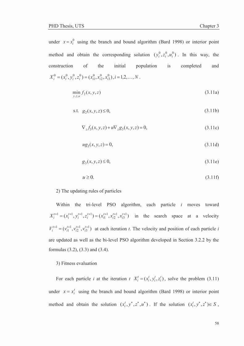
PHD Thesis, UTS Chapter 3
58
under 0ixx using the branch and bound algorithm (Bard 1998) or interior point
method and obtain the corresponding solution ),,( 000iii uzy . In this way, the
construction of the initial population is completed and
),,(),,( 03
02
01
0000iiiiiii xxxzyxX , Ni ,,2,1 .
),,(min 2,,zyxf
uzy (3.11a)
s.t. ,0),,(2 zyxg (3.11b)
,0),,(),,( 33 zyxguzyxf zz (3.11c)
,0),,(3 zyxug (3.11d)
,0),,(3 zyxg (3.11e)
.0u (3.11f)
2) The updating rules of particles
Within the tri-level PSO algorithm, each particle i moves toward
),,(),,( 13
12
11
1111 ti
ti
ti
ti
ti
ti
ti xxxzyxX in the search space at a velocity
),,( 13
12
11
1 ti
ti
ti
ti vvvV at each iteration t. The velocity and position of each particle i
are updated as well as the bi-level PSO algorithm developed in Section 3.2.2 by the
formulas (3.2), (3.3) and (3.4).
3) Fitness evaluation
For each particle i at the iteration t ),,( ti
ti
ti
ti zyxX , solve the problem (3.11)
under tixx using the branch and bound algorithm (Bard 1998) or interior point
method and obtain the solution ),,,( uzyxti . If the solution Szyxt
i ),,( ,
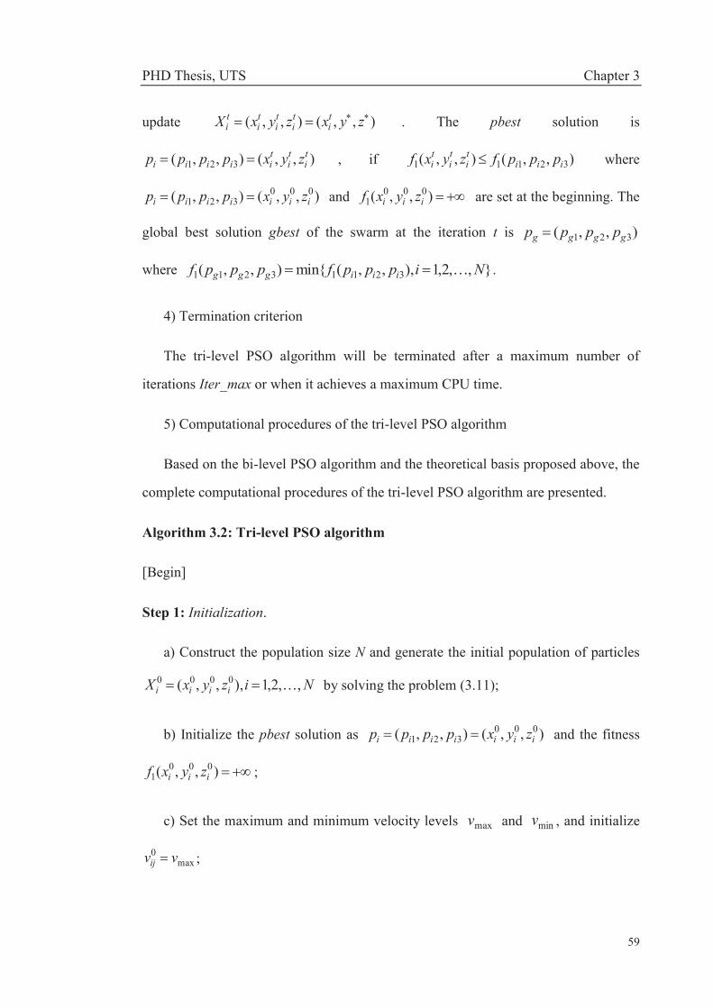
PHD Thesis, UTS Chapter 3
59
update ),,(),,( zyxzyxX ti
ti
ti
ti
ti . The pbest solution is
),,(),,( 321ti
ti
tiiiii zyxpppp , if ),,(),,( 32111 iii
ti
ti
ti pppfzyxf where
),,(),,( 000321 iiiiiii zyxpppp and ),,( 000
1 iii zyxf are set at the beginning. The
global best solution gbest of the swarm at the iteration t is ),,( 321 gggg pppp
where },,2,1),,,(min{),,( 32113211 Nipppfpppf iiiggg .
4) Termination criterion
The tri-level PSO algorithm will be terminated after a maximum number of
iterations Iter_max or when it achieves a maximum CPU time.
5) Computational procedures of the tri-level PSO algorithm
Based on the bi-level PSO algorithm and the theoretical basis proposed above, the
complete computational procedures of the tri-level PSO algorithm are presented.
Algorithm 3.2: Tri-level PSO algorithm
[Begin]
Step 1: Initialization.
a) Construct the population size N and generate the initial population of particles
NizyxX iiii ,,2,1),,,( 0000 by solving the problem (3.11);
b) Initialize the pbest solution as ),,(),,( 000321 iiiiiii zyxpppp and the fitness
),,( 0001 iii zyxf ;
c) Set the maximum and minimum velocity levels maxv and minv , and initialize
max0 vvij ;
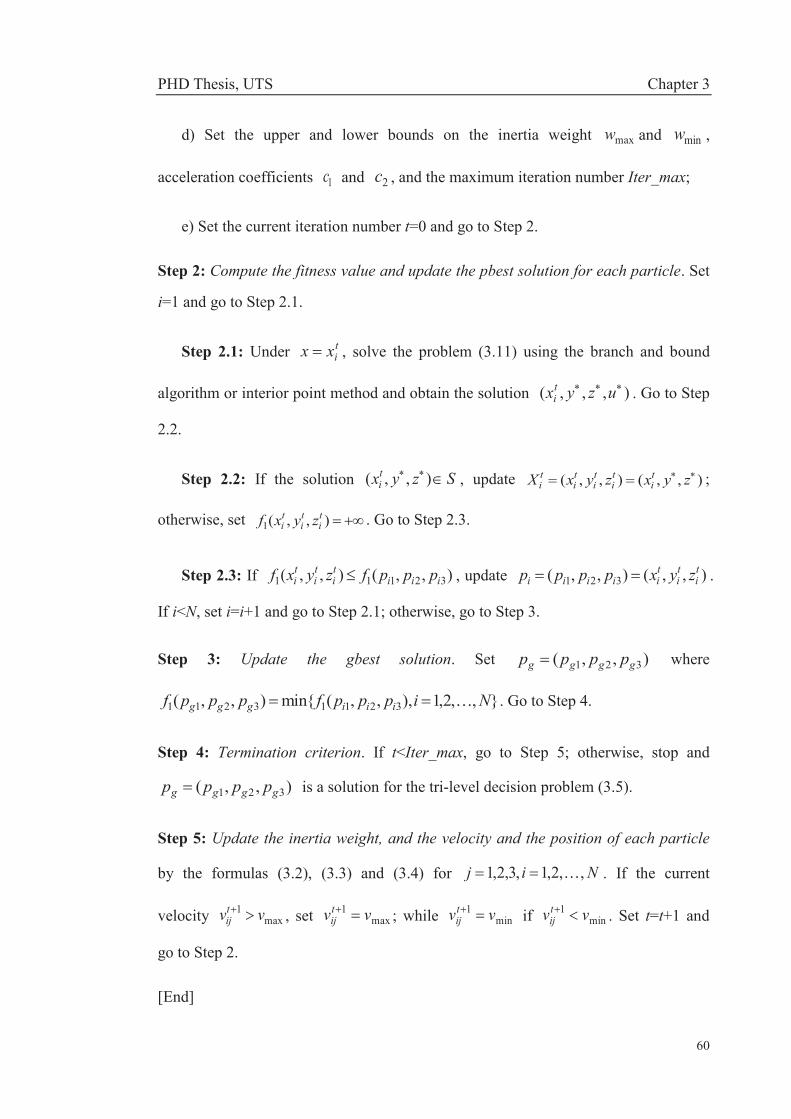
PHD Thesis, UTS Chapter 3
60
d) Set the upper and lower bounds on the inertia weight maxw and minw ,
acceleration coefficients 1c and 2c , and the maximum iteration number Iter_max;
e) Set the current iteration number t=0 and go to Step 2.
Step 2: Compute the fitness value and update the pbest solution for each particle. Set
i=1 and go to Step 2.1.
Step 2.1: Under tixx , solve the problem (3.11) using the branch and bound
algorithm or interior point method and obtain the solution ),,,( uzyxti . Go to Step
2.2.
Step 2.2: If the solution Szyxti ),,( , update ),,(),,( zyxzyxX t
iti
ti
ti
ti ;
otherwise, set ),,(1ti
ti
ti zyxf . Go to Step 2.3.
Step 2.3: If ),,(),,( 32111 iiiti
ti
ti pppfzyxf , update ),,(),,( 321
ti
ti
tiiiii zyxpppp .
If i<N, set i=i+1 and go to Step 2.1; otherwise, go to Step 3.
Step 3: Update the gbest solution. Set ),,( 321 gggg pppp where
},,2,1),,,(min{),,( 32113211 Nipppfpppf iiiggg . Go to Step 4.
Step 4: Termination criterion. If t<Iter_max, go to Step 5; otherwise, stop and
),,( 321 gggg pppp is a solution for the tri-level decision problem (3.5).
Step 5: Update the inertia weight, and the velocity and the position of each particle
by the formulas (3.2), (3.3) and (3.4) for Nij ,,2,1,3,2,1 . If the current
velocity max1 vvt
ij , set max1 vvt
ij ; while min1 vvt
ij if min1 vvt
ij . Set t=t+1 and
go to Step 2.
[End]
PHD Thesis, UTS Chapter 3
61
3.4 COMPUTATIONAL STUDY A completed computational study is conducted to show the performance of the
proposed bi-level/tri-level PSO algorithms. First, the bi-level/tri-level PSO algorithms
are applied to solve 25 bi-level and 8 tri-level benchmark problems involving linear
and nonlinear versions. Second, the bi-level PSO algorithm is applied to solve 29
large-scale nonlinear bi-level benchmark problems. Lastly, for the sake of exploring
the algorithm performance in depth, 810 large-scale bi-level decision problems are
generated using the random method proposed by Calvete, Galé and Mateo (2008). It
is noticeable that the objective value of the upper level is put in a prior position when
comparing the computational results with other algorithms. These computational
experiments are operated in MATLAB(2014a) programs performed on a 3.47GHz
Inter Xeon W3690 CPU with 12G of RAM under a Red Hat Enterprise Linux
Workstation. Also, these large-scale problems are randomly generated using the
MATLAB(2014a) environment.
3.4.1 SMALL-SCALE BENCHMARK PROBLEMS
In this section, the bi-level/tri-level PSO algorithms are applied to solve 25
bi-level and 8 tri-level benchmark problems involving linear and nonlinear versions.
Moreover, the computational results respectively obtained by the bi-level/tri-level
PSO algorithms and other algorithms are compared. The benchmark problems and
their related sources are listed in Table 3.1.
To solve the benchmark problems 1-33, related parameters involved in the
bi-level/tri-level PSO algorithms are chosen in Table 3.2. Under the parameters in
Table 3.2, the PSO algorithms are performed in 20 independent runs on each of the
above 33 benchmark problems. The computational results for bi-level decision
problems 1-25 are shown in Table 3.3. In Table 3.3, the solution and the
corresponding objective values obtained by the bi-level PSO algorithm are
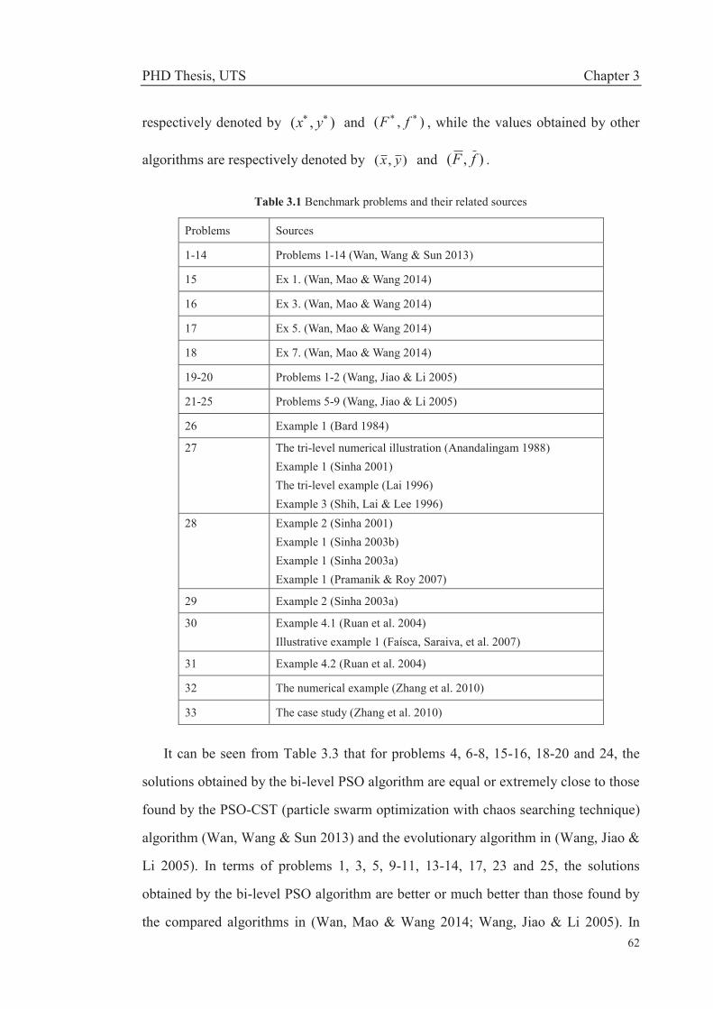
PHD Thesis, UTS Chapter 3
62
respectively denoted by ),( yx and ),( fF , while the values obtained by other
algorithms are respectively denoted by ),( yx and ),( fF .
Table 3.1 Benchmark problems and their related sources
Problems Sources
1-14 Problems 1-14 (Wan, Wang & Sun 2013)
15 Ex 1. (Wan, Mao & Wang 2014)
16 Ex 3. (Wan, Mao & Wang 2014)
17 Ex 5. (Wan, Mao & Wang 2014)
18 Ex 7. (Wan, Mao & Wang 2014)
19-20 Problems 1-2 (Wang, Jiao & Li 2005)
21-25 Problems 5-9 (Wang, Jiao & Li 2005)
26 Example 1 (Bard 1984)
27 The tri-level numerical illustration (Anandalingam 1988) Example 1 (Sinha 2001) The tri-level example (Lai 1996) Example 3 (Shih, Lai & Lee 1996)
28 Example 2 (Sinha 2001) Example 1 (Sinha 2003b) Example 1 (Sinha 2003a) Example 1 (Pramanik & Roy 2007)
29 Example 2 (Sinha 2003a)
30 Example 4.1 (Ruan et al. 2004) Illustrative example 1 (Faísca, Saraiva, et al. 2007)
31 Example 4.2 (Ruan et al. 2004)
32 The numerical example (Zhang et al. 2010)
33 The case study (Zhang et al. 2010)
It can be seen from Table 3.3 that for problems 4, 6-8, 15-16, 18-20 and 24, the
solutions obtained by the bi-level PSO algorithm are equal or extremely close to those
found by the PSO-CST (particle swarm optimization with chaos searching technique)
algorithm (Wan, Wang & Sun 2013) and the evolutionary algorithm in (Wang, Jiao &
Li 2005). In terms of problems 1, 3, 5, 9-11, 13-14, 17, 23 and 25, the solutions
obtained by the bi-level PSO algorithm are better or much better than those found by
the compared algorithms in (Wan, Mao & Wang 2014; Wang, Jiao & Li 2005). In
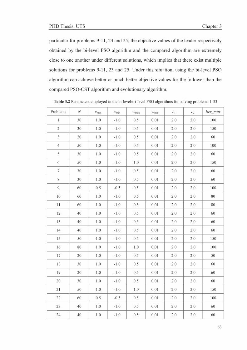
PHD Thesis, UTS Chapter 3
63
particular for problems 9-11, 23 and 25, the objective values of the leader respectively
obtained by the bi-level PSO algorithm and the compared algorithm are extremely
close to one another under different solutions, which implies that there exist multiple
solutions for problems 9-11, 23 and 25. Under this situation, using the bi-level PSO
algorithm can achieve better or much better objective values for the follower than the
compared PSO-CST algorithm and evolutionary algorithm.
Table 3.2 Parameters employed in the bi-level/tri-level PSO algorithms for solving problems 1-33
Problems N vmax vmin wmax wmin c1 c2 Iter_max 1 30 1.0 -1.0 0.5 0.01 2.0 2.0 100
2 30 1.0 -1.0 0.5 0.01 2.0 2.0 150
3 20 1.0 -1.0 0.5 0.01 2.0 2.0 60
4 50 1.0 -1.0 0.5 0.01 2.0 2.0 100
5 30 1.0 -1.0 0.5 0.01 2.0 2.0 60
6 50 1.0 -1.0 1.0 0.01 2.0 2.0 150
7 30 1.0 -1.0 0.5 0.01 2.0 2.0 60
8 30 1.0 -1.0 0.5 0.01 2.0 2.0 60
9 60 0.5 -0.5 0.5 0.01 2.0 2.0 100
10 60 1.0 -1.0 0.5 0.01 2.0 2.0 80
11 60 1.0 -1.0 0.5 0.01 2.0 2.0 80
12 40 1.0 -1.0 0.5 0.01 2.0 2.0 60
13 40 1.0 -1.0 0.5 0.01 2.0 2.0 60
14 40 1.0 -1.0 0.5 0.01 2.0 2.0 60
15 50 1.0 -1.0 0.5 0.01 2.0 2.0 150
16 80 1.0 -1.0 1.0 0.01 2.0 2.0 100
17 20 1.0 -1.0 0.5 0.01 2.0 2.0 50
18 30 1.0 -1.0 0.5 0.01 2.0 2.0 60
19 20 1.0 -1.0 0.5 0.01 2.0 2.0 60
20 30 1.0 -1.0 0.5 0.01 2.0 2.0 60
21 50 1.0 -1.0 1.0 0.01 2.0 2.0 150
22 60 0.5 -0.5 0.5 0.01 2.0 2.0 100
23 40 1.0 -1.0 0.5 0.01 2.0 2.0 60
24 40 1.0 -1.0 0.5 0.01 2.0 2.0 60
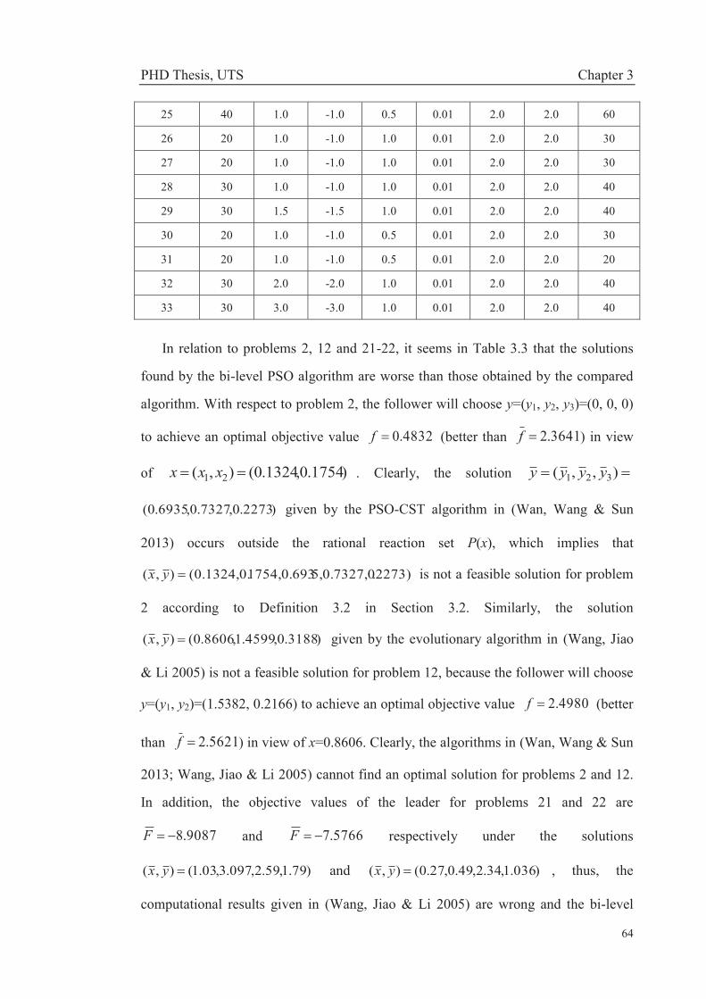
PHD Thesis, UTS Chapter 3
64
25 40 1.0 -1.0 0.5 0.01 2.0 2.0 60
26 20 1.0 -1.0 1.0 0.01 2.0 2.0 30
27 20 1.0 -1.0 1.0 0.01 2.0 2.0 30
28 30 1.0 -1.0 1.0 0.01 2.0 2.0 40
29 30 1.5 -1.5 1.0 0.01 2.0 2.0 40
30 20 1.0 -1.0 0.5 0.01 2.0 2.0 30
31 20 1.0 -1.0 0.5 0.01 2.0 2.0 20
32 30 2.0 -2.0 1.0 0.01 2.0 2.0 40
33 30 3.0 -3.0 1.0 0.01 2.0 2.0 40
In relation to problems 2, 12 and 21-22, it seems in Table 3.3 that the solutions
found by the bi-level PSO algorithm are worse than those obtained by the compared
algorithm. With respect to problem 2, the follower will choose y=(y1, y2, y3)=(0, 0, 0)
to achieve an optimal objective value 4832.0f (better than 3641.2f ) in view
of )1754.0,1324.0(),( 21 xxx . Clearly, the solution ),,( 321 yyyy
)2273.0,7327.0,6935.0( given by the PSO-CST algorithm in (Wan, Wang & Sun
2013) occurs outside the rational reaction set P(x), which implies that
.2273)5,0.7327,01754,0.693(0.1324,0.),( yx is not a feasible solution for problem
2 according to Definition 3.2 in Section 3.2. Similarly, the solution
)3188.0,4599.1,8606.0(),( yx given by the evolutionary algorithm in (Wang, Jiao
& Li 2005) is not a feasible solution for problem 12, because the follower will choose
y=(y1, y2)=(1.5382, 0.2166) to achieve an optimal objective value 4980.2f (better
than 5621.2f ) in view of x=0.8606. Clearly, the algorithms in (Wan, Wang & Sun
2013; Wang, Jiao & Li 2005) cannot find an optimal solution for problems 2 and 12.
In addition, the objective values of the leader for problems 21 and 22 are
9087.8F and 5766.7F respectively under the solutions
)79.1,59.2,097.3,03.1(),( yx and )036.1,34.2,49.0,27.0(),( yx , thus, the
computational results given in (Wang, Jiao & Li 2005) are wrong and the bi-level
PHD Thesis, UTS Chapter 3
65
PSO solutions are better than the compared algorithm for problems 21 and 22. In
general, the bi-level PSO algorithm performance better than the compared algorithms
in (Wan, Wang & Sun 2013; Wang, Jiao & Li 2005) in terms of solving problems 2,
12 and 21-22.
Table 3.4 reports the computational results for tri-level decision problems 26-33.
The solution and the corresponding objective values obtained by the tri-level PSO
algorithm are respectively denoted by ),,( zyx and ),,( 321 fff , while the values
obtained by other solution approaches are denoted by ),,( zyx and ),,( 321 fff .
Table 3.4 clearly shows that the tri-level PSO algorithm can find the same solutions as
the compared approaches or much better solutions. Note ),,( zyx that ),( zy
denotes the best reactions of the middle-level follower and the bottom-level follower
in the light of x determined by the leader. According to Definition 3.4,
),,(),,( zyxzyx under Szyx ),,( means the solution IRzyx ),,( , which
implies that ),,( zyx is a feasible solution for the tri-level decision problem;
otherwise, ),,( zyx is not a feasible solution. Thus, it can be seen from Table 3.4
that the solutions ),,( zyx in (Bard 1984) for problem 26, in (Lai 1996) for problem
27, in (Pramanik & Roy 2007; Sinha 2003a, 2003b) for problem 28, in (Faísca,
Saraiva, et al. 2007) for problem 30 and in (Zhang et al. 2010) for problem 33 are not
feasible solutions. In addition, although the solutions ),,( zyx in (Anandalingam
1988; Shih, Lai & Lee 1996) for problem 27, in (Pramanik & Roy 2007; Sinha 2001)
for problem 28 and in (Sinha 2003a) for problem 29 occurs over IR, they can be only
considered as local optimal solutions since the tri-level PSO algorithm can find much
better solutions for such problems. Thus, the tri-level PSO algorithm provides a better
way to solve tri-level decision problems.

PHD Thesis, UTS Chapter 3
66
Table 3.3 The computational results for bi-level decision problems 1-25
Problems ),( yx ),( fF ),( yx ),( fF
1 (0, 2, 1.875, 0.9063) (-18.6787, -1.0156) (0.3844, 1.6124, 1.8690, 0.8041) (-14.7772, -0.2316)
2 (0, 0.9, 0, 0.6, 0.4) (-29.2, 3.2) (0.1324, 0.1754, 0.6935, 0.7327, 0.2273) (-29.2064, 2.3641)
3 (0, 1, 0) (1000, 1) (0.1511, 0.6256, 0.369) (640.7139, 0.9946)
4 (9.9998, 9.9998) (99.996, 0) (10.0020, 9.9961) (100.0393, 0)
5 (2.0345, 0.8838, 0) (-1.2312, 7.7818) (1.8602, 0.9073, 0.005) (-1.1660, 7.4441)
6 (7.0696, 7.0696, 6.9279, 6.9278) (1.98, -1.98) (7.0321, 6.84204, 5.9071, 6.8312) (1.9816, -1.9816)
7 (20.0282, 14.8381, 0.0282, -5.1619) (0, 0) (17.5039, 29.8906, -2.4994, 9.8894) (0.0527, 0)
8 (17.8377, 20.1712, -2.1623, 0.1712) (0, 0) (12.4124, 19.3109, -7.5859, -0.6899) (0.0004, 0)
9 (20, 5, 10, 5) (0, 100) (17.2024, 7.4665, 7.2189, 2.4251) (0.0075, 125.0854)
10 (10.9317, 9.6004, 10, 9.6004) (0, 0.868) (0.1946, 14.9870, 6.1019, 7.9628) (0, 84.2367)
11 (6.4462, 11.9941, 6.4462, 10) (0, 3.9763) (10.6084, 10.0550, 9.4545, 5.1257) (0.0001, 25.6292)
12 (1.8888, 0.889, 0) (0, 7.6167) (0.8606, 1.4599, 0.3138) (0.0082, 2.5621)
13 (0.6648, 1.5746, 0.0722) (0, 2.5) (0.9099, 1.5294, 0.1762) (0.0374, 2.6969)
14 (0.6648, 1.5746, 0.0722) (0, 2.5) (0.9233, 1.5083, 0.1899) (0.0337, 2.7442)
15 (4, 15, 9.2, 2) (41.2, -9.2) (4.000517, 14.999931, 9.199862, 2) (41.199207, -9.198828)
16 (0, 30, -10, 10) (0, 100) (0, 30, -10, 10) (0, 100)
17 (1, 0) (1, 0) (10, 0) (82, 0)
18 (0, 30, -10, 10) (0, 100) (0, 30, -10, 10) (0, 100)
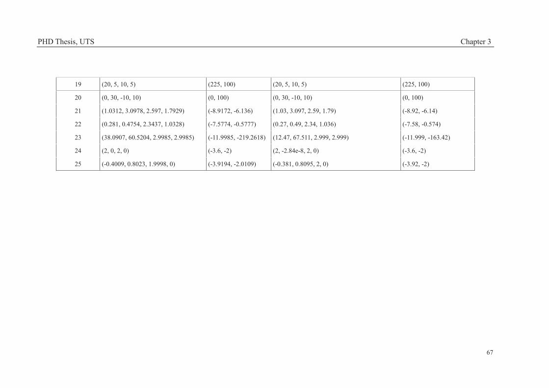
PHD Thesis, UTS Chapter 3
67
19 (20, 5, 10, 5) (225, 100) (20, 5, 10, 5) (225, 100)
20 (0, 30, -10, 10) (0, 100) (0, 30, -10, 10) (0, 100)
21 (1.0312, 3.0978, 2.597, 1.7929) (-8.9172, -6.136) (1.03, 3.097, 2.59, 1.79) (-8.92, -6.14)
22 (0.281, 0.4754, 2.3437, 1.0328) (-7.5774, -0.5777) (0.27, 0.49, 2.34, 1.036) (-7.58, -0.574)
23 (38.0907, 60.5204, 2.9985, 2.9985) (-11.9985, -219.2618) (12.47, 67.511, 2.999, 2.999) (-11.999, -163.42)
24 (2, 0, 2, 0) (-3.6, -2) (2, -2.84e-8, 2, 0) (-3.6, -2)
25 (-0.4009, 0.8023, 1.9998, 0) (-3.9194, -2.0109) (-0.381, 0.8095, 2, 0) (-3.92, -2)
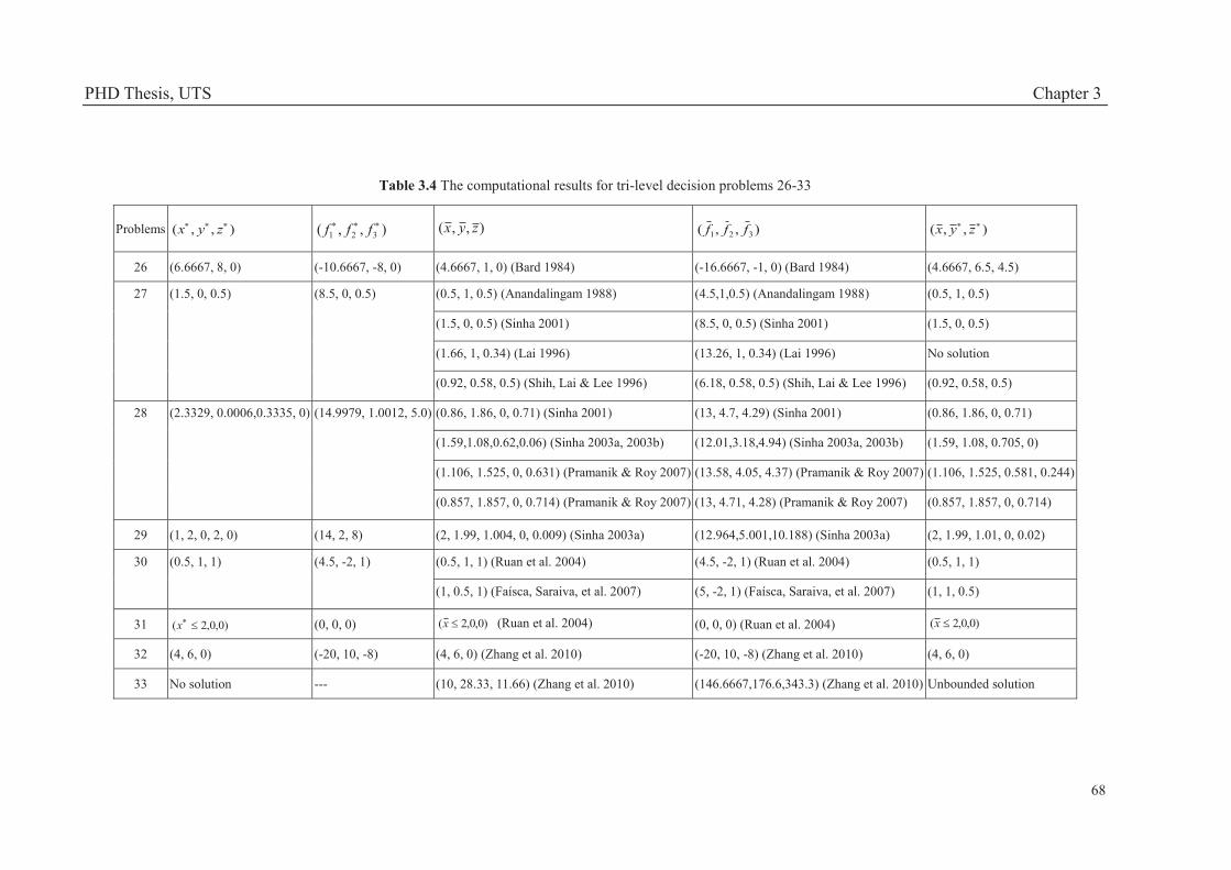
PHD Thesis, UTS Chapter 3
68
Table 3.4 The computational results for tri-level decision problems 26-33
Problems ),,( zyx ),,( 321 fff ),,( zyx ),,( 321 fff ),,( zyx
26 (6.6667, 8, 0) (-10.6667, -8, 0) (4.6667, 1, 0) (Bard 1984) (-16.6667, -1, 0) (Bard 1984) (4.6667, 6.5, 4.5)
27 (1.5, 0, 0.5) (8.5, 0, 0.5) (0.5, 1, 0.5) (Anandalingam 1988) (4.5,1,0.5) (Anandalingam 1988) (0.5, 1, 0.5)
(1.5, 0, 0.5) (Sinha 2001) (8.5, 0, 0.5) (Sinha 2001) (1.5, 0, 0.5)
(1.66, 1, 0.34) (Lai 1996) (13.26, 1, 0.34) (Lai 1996) No solution
(0.92, 0.58, 0.5) (Shih, Lai & Lee 1996) (6.18, 0.58, 0.5) (Shih, Lai & Lee 1996) (0.92, 0.58, 0.5)
28 (2.3329, 0.0006,0.3335, 0) (14.9979, 1.0012, 5.0) (0.86, 1.86, 0, 0.71) (Sinha 2001) (13, 4.7, 4.29) (Sinha 2001) (0.86, 1.86, 0, 0.71)
(1.59,1.08,0.62,0.06) (Sinha 2003a, 2003b) (12.01,3.18,4.94) (Sinha 2003a, 2003b) (1.59, 1.08, 0.705, 0)
(1.106, 1.525, 0, 0.631) (Pramanik & Roy 2007) (13.58, 4.05, 4.37) (Pramanik & Roy 2007) (1.106, 1.525, 0.581, 0.244)
(0.857, 1.857, 0, 0.714) (Pramanik & Roy 2007) (13, 4.71, 4.28) (Pramanik & Roy 2007) (0.857, 1.857, 0, 0.714)
29 (1, 2, 0, 2, 0) (14, 2, 8) (2, 1.99, 1.004, 0, 0.009) (Sinha 2003a) (12.964,5.001,10.188) (Sinha 2003a) (2, 1.99, 1.01, 0, 0.02)
30 (0.5, 1, 1) (4.5, -2, 1) (0.5, 1, 1) (Ruan et al. 2004) (4.5, -2, 1) (Ruan et al. 2004) (0.5, 1, 1)
(1, 0.5, 1) (Faísca, Saraiva, et al. 2007) (5, -2, 1) (Faísca, Saraiva, et al. 2007) (1, 1, 0.5)
31 )0,0,2(x (0, 0, 0) )0,0,2(x (Ruan et al. 2004) (0, 0, 0) (Ruan et al. 2004) )0,0,2(x
32 (4, 6, 0) (-20, 10, -8) (4, 6, 0) (Zhang et al. 2010) (-20, 10, -8) (Zhang et al. 2010) (4, 6, 0)
33 No solution --- (10, 28.33, 11.66) (Zhang et al. 2010) (146.6667,176.6,343.3) (Zhang et al. 2010) Unbounded solution
PHD Thesis, UTS Chapter 3
69
3.4.2 LARGE-SCALE BENCHMARK PROBLEMS
In this section, the bi-level PSO algorithm is applied to solve the large-scale
nonlinear bi-level decision problems 34-62. The sources of the benchmark problems
34-57 are the problems SMD1-SMD12 with five and 10 dimensions constructed by
Sinha, Malo and Deb (2014), while the problems 58-62 with 20 dimensions are cited
from the problems (Exs.12-16) solved in (Wan, Mao & Wang 2014). When solving
the problems 34-57, the population size and iteration number are chosen as N=30,
Iter_max=60 and N=50, Iter_max=100 respectively for solving five-dimensional and
10-dimensional problems. The other parameters in the bi-level PSO algorithm are
chosen as follows: vmax=1.0, vmin=-1.0, c1=c2=2, wmax=0.5, wmin=0.01. In response to
solving problems 58-62, the related parameters are chosen as vmax=0.5, vmin=-0.5,
c1=c2=2, wmax=0.5, wmin=0.01, N=30, Iter_max=100.
The computational results for the problems 34-45 and problems 46-57 are
respectively provided in Tables 3.5 and 3.6. In Tables 3.5 and 3.6, the solution and the
corresponding objective values obtained by the bi-level PSO algorithm are
respectively denoted by ),( yx and ),( fF , while the objective values obtained
by the nested bi-level evolutionary algorithm developed in (Sinha, Malo & Deb 2014)
are denoted by ),( fF . Let ),( fF be the objective values under the exact solution.
|)||,(|),( ffFFfF and |)||,(|),( ffFFfF are adopted to
reflect the accuracy of the solution respectively obtained by both of the algorithms.
The smaller number of ),( fF and ),( fF means the higher accuracy of the
solution obtained. It can be seen from Tables 3.5 and 3.6 that the bi-level PSO
algorithm is able to find a more accurate solution than the nested bi-level evolutionary
algorithm.
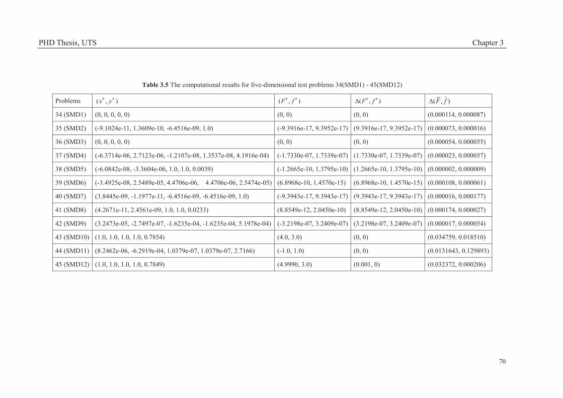
PHD Thesis, UTS Chapter 3
70
Table 3.5 The computational results for five-dimensional test problems 34(SMD1) - 45(SMD12)
Problems ),( yx ),( fF ),( fF ),( fF
34 (SMD1) (0, 0, 0, 0, 0) (0, 0) (0, 0) (0.000114, 0.000087)
35 (SMD2) (-9.1024e-11, 1.3609e-10, -6.4516e-09, 1.0) (-9.3916e-17, 9.3952e-17) (9.3916e-17, 9.3952e-17) (0.000073, 0.000016)
36 (SMD3) (0, 0, 0, 0, 0) (0, 0) (0, 0) (0.000054, 0.000055)
37 (SMD4) (-6.3714e-06, 2.7123e-06, -1.2107e-08, 1.3537e-08, 4.1916e-04) (-1.7330e-07, 1.7339e-07) (1.7330e-07, 1.7339e-07) (0.000023, 0.000057)
38 (SMD5) (-6.0842e-08, -3.3604e-06, 1.0, 1.0, 0.0039) (-1.2665e-10, 1.3795e-10) (1.2665e-10, 1.3795e-10) (0.000002, 0.000009)
39 (SMD6) (-3.4925e-08, 2.5489e-05, 4.4706e-06, 4.4706e-06, 2.5474e-05) (6.8968e-10, 1.4570e-15) (6.8968e-10, 1.4570e-15) (0.000108, 0.000061)
40 (SMD7) (3.8445e-09, -1.1977e-11, -6.4516e-09, -6.4516e-09, 1.0) (-9.3943e-17, 9.3943e-17) (9.3943e-17, 9.3943e-17) (0.000016, 0.000177)
41 (SMD8) (4.2671e-11, 2.4561e-09, 1.0, 1.0, 0.0233) (8.8549e-12, 2.0450e-10) (8.8549e-12, 2.0450e-10) (0.000174, 0.000027)
42 (SMD9) (3.2473e-05, -2.7497e-07, -1.6235e-04, -1.6235e-04, 5.1978e-04) (-3.2198e-07, 3.2409e-07) (3.2198e-07, 3.2409e-07) (0.000017, 0.000054)
43 (SMD10) (1.0, 1.0, 1.0, 1.0, 0.7854) (4.0, 3.0) (0, 0) (0.034759, 0.018510)
44 (SMD11) (8.2462e-06, -6.2919e-04, 1.0379e-07, 1.0379e-07, 2.7166) (-1.0, 1.0) (0, 0) (0.0131643, 0.129893)
45 (SMD12) (1.0, 1.0, 1.0, 1.0, 0.7849) (4.9990, 3.0) (0.001, 0) (0.032372, 0.000206)
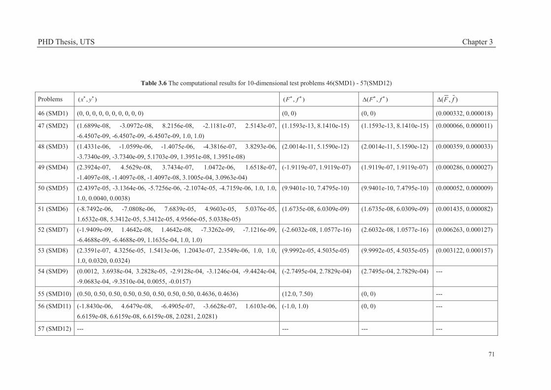
PHD Thesis, UTS Chapter 3
71
Table 3.6 The computational results for 10-dimensional test problems 46(SMD1) - 57(SMD12)
Problems ),( yx ),( fF ),( fF ),( fF
46 (SMD1) (0, 0, 0, 0, 0, 0, 0, 0, 0, 0) (0, 0) (0, 0) (0.000332, 0.000018)
47 (SMD2) (1.6899e-08, -3.0972e-08, 8.2156e-08, -2.1181e-07, 2.5143e-07, -6.4507e-09, -6.4507e-09, -6.4507e-09, 1.0, 1.0)
(1.1593e-13, 8.1410e-15) (1.1593e-13, 8.1410e-15) (0.000066, 0.000011)
48 (SMD3) (1.4331e-06, -1.0599e-06, -1.4075e-06, -4.3816e-07, 3.8293e-06, -3.7340e-09, -3.7340e-09, 5.1703e-09, 1.3951e-08, 1.3951e-08)
(2.0014e-11, 5.1590e-12) (2.0014e-11, 5.1590e-12) (0.000359, 0.000033)
49 (SMD4) (2.3924e-07, 4.5629e-08, 3.7434e-07, 1.0472e-06, 1.6518e-07, -1.4097e-08, -1.4097e-08, -1.4097e-08, 3.1005e-04, 3.0963e-04)
(-1.9119e-07, 1.9119e-07) (1.9119e-07, 1.9119e-07) (0.000286, 0.000027)
50 (SMD5) (2.4397e-05, -3.1364e-06, -5.7256e-06, -2.1074e-05, -4.7159e-06, 1.0, 1.0, 1.0, 0.0040, 0.0038)
(9.9401e-10, 7.4795e-10) (9.9401e-10, 7.4795e-10) (0.000052, 0.000009)
51 (SMD6) (-8.7492e-06, -7.0808e-06, 7.6839e-05, 4.9603e-05, 5.0376e-05, 1.6532e-08, 5.3412e-05, 5.3412e-05, 4.9566e-05, 5.0338e-05)
(1.6735e-08, 6.0309e-09) (1.6735e-08, 6.0309e-09) (0.001435, 0.000082)
52 (SMD7) (-1.9409e-09, 1.4642e-08, 1.4642e-08, -7.3262e-09, -7.1216e-09, -6.4688e-09, -6.4688e-09, 1.1635e-04, 1.0, 1.0)
(-2.6032e-08, 1.0577e-16) (2.6032e-08, 1.0577e-16) (0.006263, 0.000127)
53 (SMD8) (2.3591e-07, 4.3256e-05, 1.5413e-06, 1.2043e-07, 2.3549e-06, 1.0, 1.0, 1.0, 0.0320, 0.0324)
(9.9992e-05, 4.5035e-05) (9.9992e-05, 4.5035e-05) (0.003122, 0.000157)
54 (SMD9) (0.0012, 3.6938e-04, 3.2828e-05, -2.9128e-04, -3.1246e-04, -9.4424e-04, -9.0683e-04, -9.3510e-04, 0.0055, -0.0157)
(-2.7495e-04, 2.7829e-04) (2.7495e-04, 2.7829e-04) ---
55 (SMD10) (0.50, 0.50, 0.50, 0.50, 0.50, 0.50, 0.50, 0.50, 0.4636, 0.4636) (12.0, 7.50) (0, 0) ---
56 (SMD11) (-1.8430e-06, 4.6479e-08, -6.4905e-07, -3.6628e-07, 1.6103e-06, 6.6159e-08, 6.6159e-08, 6.6159e-08, 2.0281, 2.0281)
(-1.0, 1.0) (0, 0) ---
57 (SMD12) --- --- --- ---

PHD Thesis, UTS Chapter 3
72
Table 3.7 The computational results for 20-dimensional test problems 58-62
Problems ),( yx ),( fF ),( yx ),( fF
58 (1,1,1,1,1,1,1,1,1,1,0,0,0,0,0,0,0,0,0,0) (0,1) (1,1,1,1,1,1,1,1,1,1,0,0,0,0,0,0,0,0,0,0) (0,1)
59 (1,1,1,1,1,1,1,1,1,1,0,0,0,0,0,0,0,0,0,0) (0,1) (1,1,1,1,1,1,1,1,1,1,0,0,0,0,0,0,0,0,0,0) (0,1)
60 (-0.0859,-0.6008,0.2454,-0.1412,-1.2518, -0.1978,-0.9856,-0.1297,-0.7022,-5, 0,0,0,0,0,0,0,0,0,0)
(1.2388e-6,1) (1.149034,0.08833383,1.254797,1.182997, 2.130051, 1.742112,0.3082794, 1.591319,1.409942,-0.2195419, 0,0,0,0,0,0,0,0,0,0)
(4.64e-6,1)
61 (0.8882,0.7552,5,4.3309,-0.5017,0.8485, -1.2183,2.2813,-1.5316,0.6639, 0,0,0,0,0,0,0,0,0,0)
(1.7316e-7,1) (-1.275612,0.4240169,-1.292204,-0.57017, 1.238698,2.83057,1.313386, 0.65589,-2.799304,-1.467915)
(1.12e-5,1)
62 (1,1,1,1,1,1,1,1,1,1,0,0,0,0,0,0,0,0,0,0) (0,1) (1,1,1,1,1,1,1,1,1,1,0,0,0,0,0,0,0,0,0,0) (0,1)

PHD Thesis, UTS Chapter 3
73
Table 3.7 displays the computational results for problems 58-62 with 20
dimensions. As shown in Table 3.7, the solutions found by the bi-level PSO algorithm
are equal to those obtained by the compared algorithm in (Wan, Mao & Wang 2014)
for problems 58-59 and 62. With regard to problems 60-61, the bi-level PSO
algorithm can achieve little better in terms of objective values. Also, it can be found
from Table 3.7 that problems 60-61 have multiple solutions that can achieve objective
values extremely close to each other. To conclude, the results indicate that the bi-level
PSO algorithm can find the same solutions as the compared algorithm or better
solutions for 20-dimensional nonlinear bi-level problems.
3.4.3 ASSESSING THE EFFICIENCY PERFORMANCE OF
THE BI-LEVEL PSO ALGORITHM
This section aims to assess the efficiency performance of the proposed bi-level
PSO algorithm in relation to solve large-scale problems. In Section 3.4.2, the related
parameters employed in the bi-level PSO algorithm are provided for solving
large-scale nonlinear benchmark problems. Much less iterations need to be executed
by the bi-level PSO algorithm than the evolutionary algorithm (Sinha, Malo & Deb
2014) that needs 330 and 678 iterations at least respectively for solving
five-dimensional and 10-dimensional problems. Clearly, the bi-level PSO algorithm
has a better convergence and efficiency performance than the evolutionary algorithm
in solving large-scale nonlinear bi-level decision problems. However, the increase in
the number of decision variables (e.g. more than 20 dimensions) may result in bi-level
problems having no solutions apart from some special versions (Sinha, Malo & Deb
2014); thus, there are not sufficient benchmark nonlinear problems in the existing
research that can be used to explore the algorithm efficiency. In this study, to explore
the algorithm efficiency in solving much larger-scale (e.g. 20 dimensions or much
more) problems, the bi-level PSO algorithm is applied to solve sufficient large-scale
(40, 60 and 100 dimensions) linear bi-level problems that can be randomly generated.
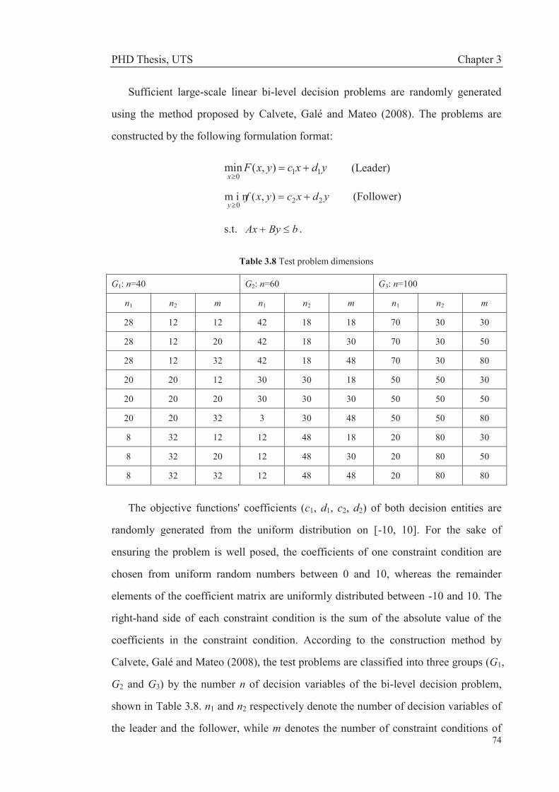
PHD Thesis, UTS Chapter 3
74
Sufficient large-scale linear bi-level decision problems are randomly generated
using the method proposed by Calvete, Galé and Mateo (2008). The problems are
constructed by the following formulation format:
ydxcyxFx 110
),(min (Leader)
ydxcyxfy 220
),(m i n (Follower)
s.t. bByAx .
Table 3.8 Test problem dimensions
G1: n=40 G2: n=60 G3: n=100
n1 n2 m n1 n2 m n1 n2 m
28 12 12 42 18 18 70 30 30
28 12 20 42 18 30 70 30 50
28 12 32 42 18 48 70 30 80
20 20 12 30 30 18 50 50 30
20 20 20 30 30 30 50 50 50
20 20 32 3 30 48 50 50 80
8 32 12 12 48 18 20 80 30
8 32 20 12 48 30 20 80 50
8 32 32 12 48 48 20 80 80
The objective functions' coefficients (c1, d1, c2, d2) of both decision entities are
randomly generated from the uniform distribution on [-10, 10]. For the sake of
ensuring the problem is well posed, the coefficients of one constraint condition are
chosen from uniform random numbers between 0 and 10, whereas the remainder
elements of the coefficient matrix are uniformly distributed between -10 and 10. The
right-hand side of each constraint condition is the sum of the absolute value of the
coefficients in the constraint condition. According to the construction method by
Calvete, Galé and Mateo (2008), the test problems are classified into three groups (G1,
G2 and G3) by the number n of decision variables of the bi-level decision problem,
shown in Table 3.8. n1 and n2 respectively denote the number of decision variables of
the leader and the follower, while m denotes the number of constraint conditions of
PHD Thesis, UTS Chapter 3
75
the bi-level problem. It can be seen from Table 3.8 that there are nine problem types
in each test problem group by different combinations of n1, n2 and m. In this
computational study, 30 test problems are randomly constructed within each problem
type; thus, there are 8103930 bi-level problems randomly generated in total
within three test problem groups.
Within the bi-level PSO algorithm, the key parameters involve the inertia weight
w, the population size N and the maximum number of iterations Iter_max. To explore
the influence of the three parameters on the performance of the bi-level PSO
algorithm, each test problem is solved under six kinds of parameter combinations of
the bi-level PSO algorithm, which involve C1 (wmax=1.0, N=100, Iter_max=300), C2
(wmax=0.75, N=100, Iter_max=300), C3 (wmax=0.50, N=100, Iter_max=300) , C4
(wmax=1.0, N=50, Iter_max=500), C5 (wmax=0.75, N=50, Iter_max=500) and C6
(wmax=0.50, N=50, Iter_max=500). In addition, other parameters within the bi-level
PSO algorithm are set as follows: vmax=5.0, vmin=-5.0, wmin=0.01, c1=c2=2. For 810
test problems, each of them is carried out 16 runs under each parameter combination.
In terms of each test problem, minF is defined as the best objective value of the
leader obtained from all parameter combinations; if the best objective value F of the
leader obtained from 16 runs under each parameter combination equals to minF , it
can be considered that the bi-level PSO algorithm can find a solution for the test
problem under the parameter combination. Table 3.9 displays the number of test
problems successfully solved under each parameter combination.

PHD Thesis, UTS Chapter 3
76
Table 3.9 The number of test problems successfully solved under each parameter combination
G1: n=40 G2: n=60 G3: n=100
n1-n2-m C1 C2 C3 C4 C5 C6 n1-n2-m C1 C2 C3 C4 C5 C6 n1-n2-m C1 C2 C3 C4 C5 C6
28-12-12 5 17 23 18 27 28 42-18-18 3 10 15 7 20 26 70-30-30 8 9 17 8 16 25
28-12-20 3 16 20 13 27 29 42-18-30 2 7 18 6 22 26 70-30-50 10 13 22 6 18 23
28-12-32 8 18 22 12 26 30 42-18-48 2 5 14 4 21 28 70-30-80 11 15 22 9 19 24
20-20-12 13 22 25 21 24 29 30-30-18 5 14 19 17 26 27 50-50-30 1 7 17 7 16 26
20-20-20 13 21 27 23 27 28 30-30-30 2 16 24 17 27 29 50-50-50 2 4 15 7 18 27
20-20-32 16 26 29 28 30 30 30-30-48 5 20 26 15 28 30 50-50-80 6 12 17 11 25 25
8-32-12 19 20 23 20 21 29 12-48-18 23 25 26 22 27 30 20-80-30 10 18 22 14 21 28
8-32-20 26 27 29 27 28 29 12-48-30 28 28 29 28 29 30 20-80-50 10 25 28 18 26 29
8-32-32 29 30 30 29 30 30 12-48-48 27 29 29 30 30 30 20-80-80 13 23 29 21 28 30
Total 132 197 228 191 240 262 Total 97 154 200 146 230 256 Total 71 126 189 101 187 237
PHD Thesis, UTS Chapter 3
77
Table 3.9 clearly shows that different combinations of the inertia weight w, the
population size N and the maximum number of iterations Iter_max have significant
influences on the performance of the bi-level PSO algorithm. As shown in Table 3.9,
most test problems are successfully solved under the parameter combination C6 within
each problem group, which means that the bi-level PSO algorithm shows higher
performance under C6 than other parameter combinations. However, the algorithm
performance under C1 - C5 becomes more and more close to that under C6 following
the decline of the number n1 of the leader's decision variables, in particular in groups
G1 and G2; Figure 3.1 clearly presents these results, which display the total number of
test problems that have the same number of the leader's decision variables
successfully solved under C1 - C6. Also, it is clear in Figure 3.1 that the algorithm
performance under each parameter combination experiences a noticeable upward
trend along with a decrease in the number n1 of the leader's decision variables within
groups G1 and G2. In terms of problem group G3, it is noticeable that the number of
test problems with n1=70 successfully solved exceeds that with n1=50, which implies
that the increase in the population size of the bi-level PSO algorithm is able to
improve its performance in solving these problems when much more decision
variables of the leader are involved.
To explore more in depth, the algorithm efficiency of the bi-level PSO algorithm
is compared with that of the genetic algorithm based on bases (GABB) developed by
Calvete, Galé and Mateo (2008) for solving these test problems randomly constructed.
The convergent CPU time and the total CPU time of all iterations completed for both
algorithms are examined in Table 3.10. Table 3.10 shows the average of the
convergent CPU time (in seconds) and the total CPU time (in seconds) for each
problem type using both algorithms. Note that the computational results of the
bi-level PSO algorithm are obtained under the parameter combination C6, while the
GABB is performed under its best related parameter combination presented by
Calvete, Galé and Mateo (2008).
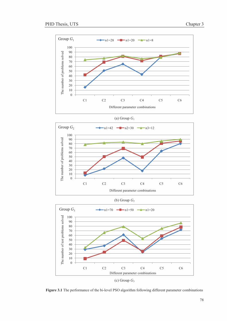
PHD Thesis, UTS Chapter 3
78
(a) Group G1
(b) Group G2
(c) Group G3
Figure 3.1 The performance of the bi-level PSO algorithm following different parameter combinations
0102030405060708090
100
C1 C2 C3 C4 C5 C6
The
num
ber o
f pro
blem
s sol
ved
Different parameter combinations
Group G1 n1=28 n1=20 n1=8
0102030405060708090
100
C1 C2 C3 C4 C5 C6
The
num
ber o
f pro
blem
s sol
ved
Different parameter combinations
Group G2 n1=42 n2=30 n3=12
0102030405060708090
100
C1 C2 C3 C4 C5 C6
The
num
ber o
f tes
t pro
blem
s sol
ved
Different parameter combinations
Group G3 n1=70 n1=50 n1=20

PHD Thesis, UTS Chapter 3
79
Table 3.10 The computational results respectively obtained by the bi-level PSO algorithm and GABB
Test Problems PSO GABB
Group n1-n2-m Convergent iteration number Convergent time (s) Total time (s) Convergent time (s) Total time (s)
G1 28-12-12 356.03 45.34 74.22 4.92 27.32
28-12-20 376.38 49.28 64.48 10.49 33.65
28-12-32 344.50 59.35 84.90 13.85 41.26
20-20-12 360.97 47.21 66.92 7.31 39.25
20-20-20 365.39 52.28 72.57 11.58 51.36
20-20-32 353.80 60.82 87.52 20.29 67.35
8-32-12 265.48 72.58 136.15 13.75 72.10
8-32-20 240.28 68.97 137.76 19.34 82.65
8-32-32 237.50 80.64 169.46 38.52 110.65
G2 42-18-18 365.38 47.54 63.58 12.68 56.38
42-18-30 370.81 51.27 69.68 20.96 71.84
42-18-48 397.96 60.49 74.36 32.29 95.43
30-30-18 366.52 54.18 73.87 21.03 105.57
30-30-30 368.03 53.69 73.09 38.35 128.64
30-30-48 383.47 62.36 81.26 59.31 169.91
12-48-18 351.53 92.03 129.38 68.62 284.05
12-48-30 358.03 95.11 135.48 108.24 361.54
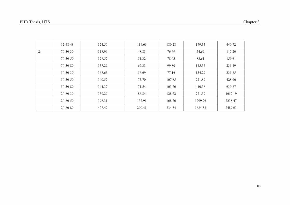
PHD Thesis, UTS Chapter 3
80
12-48-48 324.50 116.66 180.28 179.35 440.72
G3 70-30-30 318.96 48.83 76.69 54.69 115.20
70-30-50 328.52 51.32 78.05 83.61 159.61
70-30-80 337.29 67.33 99.80 145.37 231.49
50-50-30 368.65 56.69 77.16 134.29 331.85
50-50-50 340.52 75.70 107.85 221.89 428.96
50-50-80 344.32 71.54 103.76 410.36 630.87
20-80-30 339.29 86.84 128.72 771.59 1652.19
20-80-50 396.31 132.91 168.76 1299.76 2238.47
20-80-80 427.47 200.41 234.34 1684.53 2489.63

PHD Thesis, UTS Chapter 3
81
(a) Group G1
(b) Group G2
(c) Group G3
Figure 3.2 The average of the convergent CPU time
0102030405060708090
The
conv
erge
d C
PU ti
me
n1-n2-m
Group G1 PSO GABB
020406080
100120140160180200
The
conv
erge
d C
PU ti
me
n1-n2-m
Group G2 PSO GABB
0200400600800
10001200140016001800
The
conv
erge
d C
PU ti
me
n1-n2-m
Group G3 PSO GABB

PHD Thesis, UTS Chapter 3
82
(a) Group G1
(b) Group G2
(c) Group G3
Figure 3.3 The average of the total CPU time of all iterations completed
020406080
100120140160180
The
tota
l CPU
tim
e
n1-n2-m
Group G1 PSO GABB
050
100150200250300350400450500
The
tota
l CPU
tim
e
n1-n2-m
Group G2 PSO GABB
0500
10001500200025003000
The
tota
l CPU
tim
e
n1-n2-m
Group G3 PSO GABB

PHD Thesis, UTS Chapter 3
83
It can be seen from Table 3.10 that the bi-level PSO algorithm spends more CPU
times obtaining the best solution and completing all iterations for solving problem
group G1, however, both CPU times of the bi-level PSO algorithm become less and
less than GABB following the increase in the number of decision variables within
problem groups G2 and G3; Figure 3.2 and Figure 3.3 display much more evident
results. Figure 3.2 and Figure 3.3 clearly show that both the convergent and total CPU
times of GABB increase steeply with the increase in the size of the test problems. In
particular in group G3, GABB takes much more CPU times than the bi-level PSO
algorithm to converge to the best solution and complete all the iterations, which
implies that the bi-level PSO algorithm has a significant advantage in solving
larger-scale problems.
3.5 SUMMARY In this chapter, a bi-level PSO algorithm is developed to solve nonlinear and
large-scale bi-level decision problems, whereas the algorithm is then extended to a
tri-level PSO algorithm for solving tri-level decision problems. In the proposed
bi-level/tri-level PSO algorithms, the leader's problem and the follower's problem are
separated based on related solution concepts for solving conveniently. To handle the
complexity of the constraint region of nonlinear and large-scale problems, two
methods for constructing the initial population are given. Moreover, the decreasing
inertia weight with time is used to control the velocity of particles in the search space
at different stages, which aims to improve both search and convergence abilities of
the bi-level/tri-level PSO algorithms.
To illustrate the effectiveness of the proposed bi-level/tri-level PSO algorithms,
the algorithms are applied to solve 62 benchmark problems from references and 810
large-scale problems which are randomly constructed. The computational results are
compared with those obtained by the existing PSO-CST algorithm (Wan, Wang &
Sun 2013), evolutionary algorithms (Sinha, Malo & Deb 2014; Wan, Mao & Wang
2014; Wang, Jiao & Li 2005) and genetic algorithm (Calvete, Galé & Mateo 2008).

PHD Thesis, UTS Chapter 3
84
On the one hand, the computational results of these benchmark bi-level and tri-level
decision problems report that the bi-level/tri-level PSO algorithms are able to find
much better solutions than the compared algorithms. On the other hand, the
computational results of these large-scale problems clearly indicate that the bi-level
PSO algorithm shows much better performance in terms of efficiency than the
compared algorithms following the problem size becoming larger and larger. In
conclusion, the proposed bi-level PSO algorithm provides a practical way to solve
nonlinear and large-scale bi-level decision problems; also, it can be extended to a
tri-level PSO algorithm for solving tri-level decision problems.

PHD Thesis, UTS Chapter 4
85
CHAPTER 4 COMPROMISE-BASED
FUZZY NONLINEAR BI-LEVEL
DECISION MAKING
4.1 INTRODUCTION An important issue in modeling and solving a bi-level decision problem is that
parameters involved are sometimes obtained through experiments or experts'
understanding of the nature of the parameters, which are often imprecisely or
ambiguously known to decision entities; clearly, it is not reasonable to describe these
parameters by precise values (Zhang, Lu & Gao 2015). With this observation, it
would be certainly more appropriate to interpret the experts' understanding of such
parameters as fuzzy numerical data that can be represented by means of fuzzy set
theory. A bi-level decision problem in which the parameters are described by fuzzy
values, often characterized by fuzzy numbers, is called a fuzzy bi-level decision
problem (Zhang & Lu 2007).
Although numerous solution approaches have been developed to solve fuzzy
bi-level decision problems, these solution approaches have the following limitations:
(1) limited to handling linear problems involving special fuzzy numbers, such as
triangular fuzzy number; (2) limited to solving fuzzy linear decision problems in a
special situation where all of the decision entities share the same constraint conditions.
Consequently, further investigation into solution approaches is necessary for solving
nonlinear bi-level decision problems involving general fuzzy numbers.

PHD Thesis, UTS Chapter 4
86
This chapter aims to provide an effective algorithm for solving fuzzy nonlinear
bi-level decision problems. It first presents a general fuzzy bi-level decision problem
which can be transformed into a crisp problem by a commonly used fuzzy number
ranking method proposed by Jiménez (1996). The solution to the crisp problem varies
with different identifications of fuzzy decision conditions by the leader and follower;
in this situation, the leader and follower need to achieve a compromised selection of
fuzzy decision conditions to obtain an acceptable optimal solution. Based on rules of
compromise between the leader and the follower under fuzziness, the bi-level PSO
algorithm in Chapter 3 is then extended to solve the proposed fuzzy nonlinear bi-level
decision problem, called the compromise-based PSO algorithm. Lastly, numerical
examples are used to illustrate the effectiveness of the proposed solution approach.
This chapter is organized as follows. Following the introduction, Section 4.2
presents related preliminaries of fuzzy set theory which are used in this chapter. In
Section 4.3, a general fuzzy nonlinear bi-level decision problem and related
theoretical properties are proposed. In Section 4.4, the compromise-based PSO
algorithm is developed. The proposed PSO algorithm is used to solve numerical
examples in Section 4.5. A summary is given in Section 4.6.
4.2 PRELIMINARIES OF FUZZY SET THEORY This section presents related notations and definitions of fuzzy set theory that are
used in the subsequent sections.
Definition 4.1 (Heilpern 1992) The membership function of a fuzzy number a~
can be described in the following manner:
),,[],,[],,[],,[],,(
0)(
1)(
0
)(
4
43
32
21
1
~
axaaxaaxaaxax
xg
xfxr
a
a
a
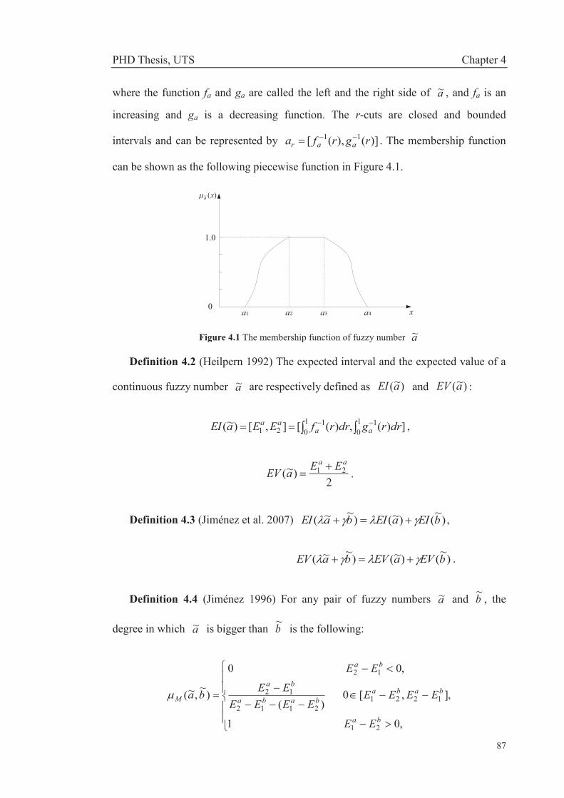
PHD Thesis, UTS Chapter 4
87
where the function fa and ga are called the left and the right side of a~ , and fa is an
increasing and ga is a decreasing function. The r-cuts are closed and bounded
intervals and can be represented by )](),([ 11 rgrfa aar . The membership function
can be shown as the following piecewise function in Figure 4.1.
a1 a4a2 a3 x
)(~ xa
0
1.0
Figure 4.1 The membership function of fuzzy number a~
Definition 4.2 (Heilpern 1992) The expected interval and the expected value of a
continuous fuzzy number a~ are respectively defined as )~(aEI and )~(aEV :
])(,)([],[)~( 10
110
121 drrgdrrfEEaEI aaaa ,
2)~( 21
aa EEaEV .
Definition 4.3 (Jiménez et al. 2007) )~()~()~~( bEIaEIbaEI ,
)~()~()~~( bEVaEVbaEV .
Definition 4.4 (Jiménez 1996) For any pair of fuzzy numbers a~ and b~ , the
degree in which a~ is bigger than b~ is the following:
,01
],,[0)(
,00
)~,~(
21
12212112
12
12
ba
babababa
ba
ba
M
EE
EEEEEEEE
EE
EE
ba
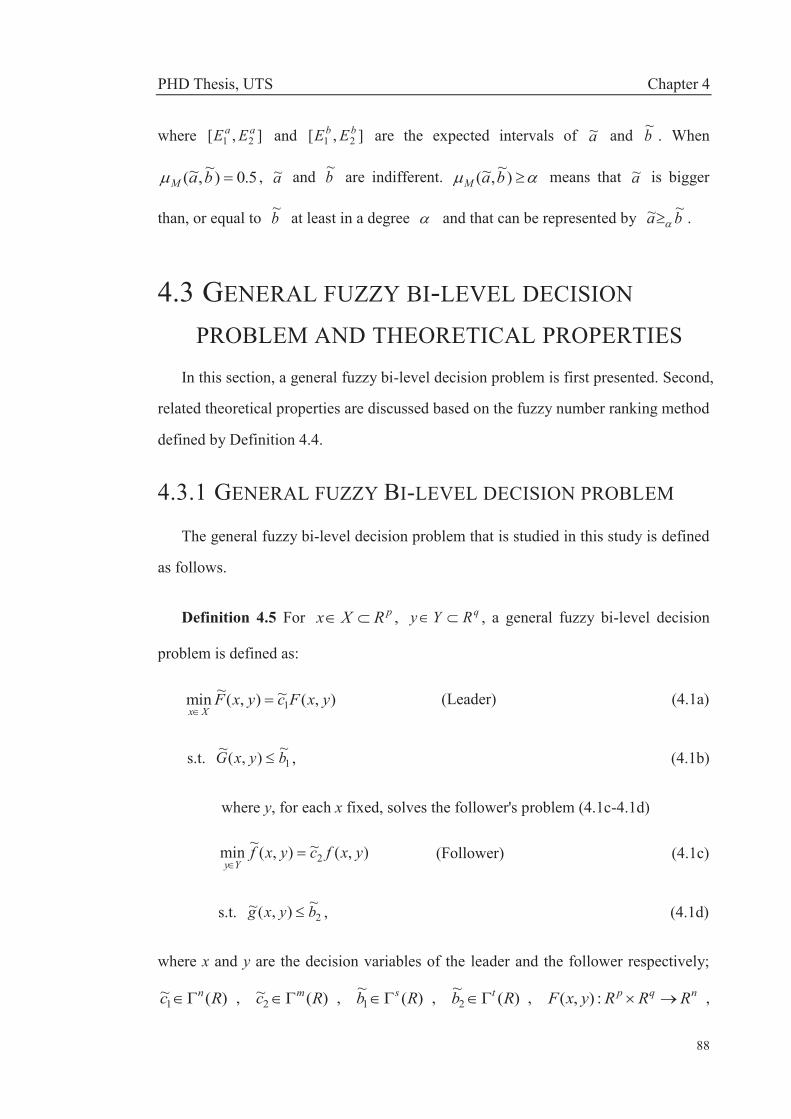
PHD Thesis, UTS Chapter 4
88
where ],[ 21aa EE and ],[ 21
bb EE are the expected intervals of a~ and b~ . When
5.0)~,~( baM , a~ and b~ are indifferent. )~,~( baM means that a~ is bigger
than, or equal to b~ at least in a degree and that can be represented by ba ~~ .
4.3 GENERAL FUZZY BI-LEVEL DECISION
PROBLEM AND THEORETICAL PROPERTIES In this section, a general fuzzy bi-level decision problem is first presented. Second,
related theoretical properties are discussed based on the fuzzy number ranking method
defined by Definition 4.4.
4.3.1 GENERAL FUZZY BI-LEVEL DECISION PROBLEM
The general fuzzy bi-level decision problem that is studied in this study is defined
as follows.
Definition 4.5 For pRXx , qRYy , a general fuzzy bi-level decision
problem is defined as:
),(~),(~min 1 yxFcyxFXx
(Leader) (4.1a)
s.t. 1~),(~ byxG , (4.1b)
where y, for each x fixed, solves the follower's problem (4.1c-4.1d)
),(~),(~min 2 yxfcyxfYy
(Follower) (4.1c)
s.t. 2~),(~ byxg , (4.1d)
where x and y are the decision variables of the leader and the follower respectively;
)(~1 Rc n , )(~
2 Rc m , )(~1 Rb s , )(~
2 Rb t , nqp RRRyxF :),( ,

PHD Thesis, UTS Chapter 4
89
mqp RRRyxf :),( , )(:),(~ RRRyxF qp , )(:),(~ RRRyxf qp ,
)(:),(~ RRRyxG sqp , )(:),(~ RRRyxg tqp , )(R is the set of all finite
fuzzy numbers.
To find an acceptable optimal solution to the fuzzy bi-level decision problem (4.1),
solution concepts in relation to operations of the fuzzy bi-level decision-making
process are presented as follows:
Definition 4.6
(1) The constraint region of the fuzzy bi-level decision problem (4.1):
}~),(~,~),(~:),{( 21 byxgbyxGYXyxS .
(2) The feasible set of the follower for each fixed x:
}~),(~:{)( 2byxgYyxS .
(3) The rational reaction set of the follower:
)]}(:),(~min[arg:{)( xSyyxfyYyxP .
(4) The inducible region of the fuzzy bi-level decision problem (4.1):
)}(,),(:),{( xPySyxyxIR .
(5) The optimal solution set of the fuzzy bi-level decision problem (4.1):
]}),(:),(~min[arg),(:),{( IRyxyxFyxyxOS .
It is clear from Definition 4.6 that the fuzzy bi-level decision-making process
involves uncertain parameters compared with crisp problems. However, the
operations of both fuzzy and crisp decision-making process are the same as each
other.

PHD Thesis, UTS Chapter 4
90
4.3.2 RELATED THEORETICAL PROPERTIES
To handle fuzzy parameters involved and develop an effective solution algorithm,
this section discusses related theoretical properties of the fuzzy bi-level decision
problem (4.1) based on fuzzy set theory.
Definition 4.7 Given a decision vector ),( yx , it is said to be feasible in a degree
( -feasible) to the constraint region S if
))},(~,~()),,(~,~(min{ 21 yxgbyxGb MM . (4.2)
In view of Definition 4.4, the previous expression (4.2) can be written as :
111212 )1()1( bbGG EEEE ,
221212 )1()1( bbgg EEEE .
The -feasible constraint region of the fuzzy bi-level decision problem (4.1) can
be denoted by
,)1()1(:),{( 111212bbGG EEEEYXyxS
})1()1( 221212bbgg EEEE .
By Definition 4.7, if 21 , then SS21
.
In line with Definition 4.7, let LM yxGb )},(~,~(min{ 1 and
FM yxgb )},(~,~(min{ 2 , thus, },min{ FL . For the fixed x by the leader, y
can be said to be F -feasible to the feasible set of the follower S(x) under
FM yxgb )},(~,~(min{ 2 . Accordingly, the feasible set of the follower in relation to
all F -feasible decision vectors can be denoted by:

PHD Thesis, UTS Chapter 4
91
})1()1(:{)( 221212b
Fb
Fg
Fg
F EEEEYyxSF
,
and the F -feasible rational reaction set of the follower can be written as:
)]}(:),(~min[arg:{)( xSyyxfyYyxPFF
. (4.3)
Thus, the -feasible inducible region of the fuzzy bi-level problem (4.1) is:
)}(,),(:),{( xPySyxyxIRF
.
Definition 4.8 For each given x by the leader, y is said to be an acceptable
optimal solution to the problem )}(:),(~min{ xSyyxfF
if it is verified that:
5.0)),(~),,(~( yxfyxfM for )(xSyF
.
By Definition 4.4,
),(~),(~5.0 yxfyxf for )(xSy
F (4.4)
can be easily obtained, which means that y is a better choice of the follower at
least in degree 0.5 as opposed to the other feasible solutions in )(xSF
. Using the
Definition 4.3, the previous expression (4.4) can be written as:
5.0)( ),(~
2),(~
1),(~
1),(~
2
),(~
1),(~
2yxfyxfyxfyxf
yxfyxf
EEEEEE
or
22
),(~
1),(~
2),(~
1),(~
2yxfyxfyxfyxf EEEE .
In view of Definition 4.2 and Definition 4.3, the expression allows us to set the
following proposition:

PHD Thesis, UTS Chapter 4
92
Proposition 4.1 For each fixed x , y is an F -acceptable optimal solution to
the second-level problem )}(:),(~min{ xSyyxf if it is an optimal solution to the
following crisp problem:
)}(:)),(~(min{ xSyyxfEVF
)}(:),()~(min{ 2 xSyyxfcEVF
, (4.5)
where )()~( 2 RFcEV m is the expected value of the fuzzy vector 2~c .
By Proposition 4.1, the expression (4.3) can be written as
)]}(:),()~(min[arg:{)( 2 xSyyxfcEVyYyxPFF
. Similarly, the following
Proposition 4.2 is obtained.
Proposition 4.2 ),( oo yx is an -acceptable optimal solution to the fuzzy
bi-level decision problem (4.1) if it is an optimal solution to the following crisp
problem:
}),(:)),(~(min{ IRyxyxFEV }),(:),()~(min{ 1 IRyxyxFcEV , (4.6)
where )()~( 1 RFcEV n is the expected value of the fuzzy vector 1~c .
In the light of the proposed definitions and propositions, an optimal solution to the
fuzzy bi-level decision problem (4.1) can be found under the minimal feasible degrees
and F respectively preferred by the leader and the follower; the solution
obtained is considered as at least an -acceptable optimal solution where F .
However, to find a solution to the fuzzy bi-level decision problem (4.1), two
conflicting factors need to be taken into account: the acceptable value for the
objective functions and the feasible degree for the constraint conditions. On the one
hand, for each fixed x, the objective value of the follower will become worse
following the increase in the feasible degree F . On the other hand, for all solutions
PHD Thesis, UTS Chapter 4
93
IRyx ),( , the objective value of the leader also becomes worse with the feasible
degree going up. Thus, the optimal solution obtained depends on the selection of
the minimal feasible degrees and F .
4.4 COMPROMISE-BASED PSO ALGORITHM Different selections of and F by the leader and the follower result to
changes of the constraint region and inducible region, which will generate different
solutions and related objective values. It is the fact that different selections of and
F keep the feature of uncertainty of the fuzzy bi-level decision problem, although it
has been transformed in to a crisp problem using fuzzy set theory. Within the
decision-making process, decision entities can choose values of and F by
communicating and consulting with one another in line with different decision
environments; this is called compromise-based rules. Under compromise-based rules,
decision entities can not only achieve the preferred optimal solution in specific
decision situations, but also obtain different solutions due to various decision
environments.
This section employs compromise-based rules to deal with the selection and
F . Also, the bi-level PSO algorithm presented in Chapter 3 is extended to obtain
optimal solutions in relation to different compromised selections of and F .
Note that if the leader and the follower share the same constraint conditions in
problem (4.1), F must be made to ensure the leader and the follower having
the same identification towards the shared constraint conditions.
In the compromise-based PSO algorithm, related definitions of swarm, particles,
pbest solution and gbest solution are the same as the bi-level PSO algorithm in
Chapter 3. In a swarm with the size N, the position vector of each particle with index i
PHD Thesis, UTS Chapter 4
94
),,2,1( Ni is denoted as ),( ti
ti
ti yxX at iteration t, which represents a
potential solution to the problem (4.1). For the sake of convenient discussion, let
),(),( 21ti
ti
ti
ti
ti xxyxX . At iteration t, each particle i moves from t
iX to 1tiX in
the search space at a velocity ),( 12
11
1 ti
ti
ti vvV along each dimension. Each particle
keeps track of its coordinates in hyperspace which are associated with the best
solution (fitness), called pbest solution ( ),( 21 iii ppp ). The particle swarm optimizer
keeps track of the overall best value, called gbest solution ( ),( 21 ggg ppp ).
(1) Initial population
In an initial population of particles with the number N , each particle i
),,2,1( Ni can be represented as ),(),( 02
01
000iiiii xxyxX . An initial population
is randomly constructed with the size N, where 0iX is randomly generated in S
by setting 0 .
(2) The updating rules of particles
The updating rules of particles in this compromise-based PSO algorithm are the
same as the rules proposed in Section 3.2.2 of Chapter 3.
3) Fitness evaluation
For each particle i at the iteration t ),( ti
ti
ti yxX , adopt the existing simplex
method or interior point method to solve the problem (4.5) under tixx and
*FF specified by the follower using the existing simplex method or interior
point method, then obtain the solution ),( yxti where )( t
ixPyF
and update
),(),( yxyxX ti
ti
ti
ti . If L
ti
tiM yxGb )},(~,~(min{ 1 where is specified
by the leader, then )( ti
ti xPy
F and Syx t
iti ),( , which means IRyx t
iti ),( ;

PHD Thesis, UTS Chapter 4
95
that is, ),( ti
ti yx is at least a -acceptable feasible solution to the fuzzy bi-level
decision problem (4.1). The pbest solution is ),(),( 21ti
tiiii yxppp and the exact
feasible degree for the constraint region S is },min{)( FLip , if
)),(~()),(~( 21 iiti
ti ppFEVyxFEV where ),(),( 00
21 iiiii yxppp ,
)),(~( 21 ii ppFEV and 0)( ip are set at the beginning. The global best
solution gbest of the swarm is ),( 21 ggg ppp and the corresponding feasible
degree for the constraint region S is )( gp where
},,2,1)),,(~(min{)),(~( 2121 NippFEVppFEV iigg .
Clearly, ),( 21 ggg ppp is an -acceptable optimal solution to the fuzzy
bi-level problem (4.1).
(4) Termination criterion
The compromise-based PSO algorithm will be terminated after a maximum
number of iterations Iter_max or when it achieves a maximum CPU time.
(5) Computational procedures of the compromise-based PSO algorithm
Based on the theoretical basis proposed above, the complete computational
procedures of the compromise-based PSO algorithm is presented for solving the fuzzy
bi-level decision problem (4.1).
Algorithm 4.1: Compromise-based PSO algorithm
[Begin]
Step 1: Initialization.
a) Construct the population size N and generate the initial population of particles
NiyxX iii ,,2,1),,( 000 ;

PHD Thesis, UTS Chapter 4
96
b) Initialize the pbest solution ),(),( 0021 iiiii yxppp , the fitness
))(~( ipFEV and the feasible degrees for the constraint conditions *FF ,
and 0)( ip ;
c) Set the maximum and minimum velocity levels maxv and minv , and initialize
max0 vvij ;
d) Set the upper and lower bounds on the inertia weight maxw and minw ,
acceleration coefficients 1c and 2c , and the maximum iteration number Iter_max;
e) Set the current iteration number t=0 and go to Step 2.
Step 2: Compute the fitness value and update the pbest solution for each particle. Set
i=1 and go to Step 2.1.
Step 2.1: Under tixx , solve the problem (4.5) under t
ixx and *FF
using the existing simplex method or interior point method, obtain the solution
),( yxti and update ),(),( yxyxX t
iti
ti
ti . Go to Step 2.2.
Step 2.2: If Lti
tiM yxGb )},(~,~(min{ 1 , go to Step 2.3; otherwise, go to
Step 2.4.
Step 2.3: If )),(~()),(~( 21 iiti
ti ppFEVyxFEV or )),(~()),(~( 21 ii
ti
ti ppfEVyxfEV
under )),(~()),(~( 21 iiti
ti ppFEVyxFEV , update ),(),( 21
ti
tiiii yxppp and
},min{)( FLip . Go to Step 2.4.
Step 2.4: If i<N, set i=i+1 and go to Step 2.1; otherwise, go to Step 3.
Step 3: Update the gbest solution. Set ),( 21 ggg ppp and )( gp where
},,2,1)),,(~(min{)),(~( 2121 NippFEVppFEV iigg . Go to Step 4.

PHD Thesis, UTS Chapter 4
97
Step 4: Termination criterion. If t<Iter_max, go to Step 5; otherwise, stop and
),( 21 ggg ppp is an -acceptable optimal solution to the fuzzy bi-level decision
problem (4.1).
Step 5: Update the inertia weight, and the velocity and the position of each particle
by the formulas (3.2), (3.3) and (3.4) in Chapter 3. If the current velocity max1 vvt
ij ,
set max1 vvt
ij ; while min1 vvt
ij if min1 vvt
ij . Set t=t+1 and go to Step 2.
[End]
4.5 NUMERICAL EXAMPLES This section first illustrates how the proposed PSO algorithm works through
solving a fuzzy nonlinear bi-level decision problem in which the fuzzy numbers are
characterized by nonlinear membership functions. Second, the PSO algorithm is used
to solve two benchmark problems and the computational results are compared with
that obtained by the existing algorithms.
4.5.1 AN ILLUSTRATIVE EXAMPLE
Consider the following fuzzy nonlinear bi-level decision problem (4.7):
221
22
21 1~4~3~1~),(~min yyxxyxF
x (Leader) (4.7a)
s.t. 4~2~1~ 221 xx , (4.7b)
0x , (4.7c)
where y, for each x fixed, solves the follower's problem (4.7d-4.7g)
221
21 5~1~2~),(~min yyxyxf
y (Follower) (4.7d)
s.t. 3~1~2~1~2~1~ 21221
21 yyxxx , (4.7e)

PHD Thesis, UTS Chapter 4
98
4~4~3~1~ 212 yyx , (4.7f)
0y . (4.7g)
The membership functions of the coefficients in this example are given as
follows:
20
213
4
10
00
)( 2
2
1~
t
tt
tt
t
t ,
30
325
9
213
1
10
)(2
2
2~
t
tt
tt
t
t ,
40
437
16
325
4
20
)(2
2
3~
t
tt
tt
t
t ,
50
549
25
437
9
30
)(2
2
4~
t
tt
tt
t
t ,
60
6511
36
549
16
40
)(2
2
5~
t
tt
tt
t
t .
Whereas the existing solution approaches cannot be adopted to solve the fuzzy
nonlinear bi-level decision problem, the compromise-based PSO algorithm is used to
find acceptable optimal solutions for the problem. Based on the PSO procedures
developed in Section 4.4, the related parameters involved in the algorithm are
initialized in Table 4.1.
Table 4.1 Parameters employed in the compromise-based PSO algorithm for solving problem (4.7)
N vmax vmin wmax wmin c1 c2 Iter_max 30 1.0 -1.0 0.5 0.01 2.0 2.0 60

PHD Thesis, UTS Chapter 4
99
Table 4.2 The computational results of problem (4.7) under different compromised conditions
F (x, y) ))~
(),~(( fEVFEV Iterations
0.5 0.5 (0.0014, 1.9669, 1.7003, 0.8241) (-17.7991, -0.9220) 0.5 39
0.6 (0.0010, 1.9669, 1.6050, 0.6290) (-17.7309, -0.2933) 0.5 32
0.7 (0.0016, 1.9669, 1.5142, 0.4506) (-17.5797, 0.2870) 0.5 35
0.8 (0.0002, 1.9669, 1.4276, 0.2872) (-17.3653, 0.8235) 0.5 39
0.9 (0.0001, 1.9669, 1.3448, 0.1374) (-17.1032, 1.3202) 0.5 31
1.0 (0, 1.9669, 1.2672, 0.0007) (-16.8121, 1.7809) 0.5 38
0.6 0.6 (0.0003, 1.8307, 1.6050, 0.5952) (-16.2103, -0.1238) 0.6 33
0.7 (0.0005, 1.8307, 1.5142, 0.4205) (-16.0423, 0.4381) 0.6 32
0.8 (0.0011, 1.8307, 1.4276, 0.2606) (-15.8149, 0.9571) 0.6 44
0.9 (0.0009, 1.8307, 1.3448, 0.1141) (-15.5432, 1.4371) 0.6 37
1.0 (0.0018, 1.8307, 1.3019, 0) (-15.3852, 1.8832) 0.6 36
0.7 0.7 (0.0009, 1.7063, 1.5142, 0.3930) (-14.7354, 0.5761) 0.7 46
0.8 (0.0039, 1.7063, 1.4276, 0.2363) (-14.4965, 1.0790) 0.7 29
0.9 (0.0051, 1.7063, 1.3448, 0.0928) (-14.2162, 1.5438) 0.7 41
1.0 (0.0008, 1.7063, 1.3346, 0) (-14.1848, 1.9790) 0.7 47
0.8 0.8 (0.0004, 1.5924, 1.4276, 0.2140) (-13.3696, 1.1907) 0.8 36
0.9 (0.0035, 1.5924, 1.3448, 0.0734) (-13.0817, 1.6414) 0.8 36
1.0 (0.0097,1.5924, 1.3646, 0) (-13.1667, 2.0692) 0.8 46
0.9 0.9 (0.0009, 1.4877, 1.3448, 0.0555) (-12.1071, 1.7313) 0.9 38
1.0 (0.0110, 1.4875, 1.3922, 0) (-12.3000,2.1537) 0.9 30
1.0 1.0 (0.0544, 1.3708, 1.4229, 0) (-11.4164, 2.2556) 1.0 48
The PSO algorithm is implemented in MATLAB R2014a. The computational
results under different compromised selections of and F are reported in Table
4.2. In Table 4.2, the first column and the second column F are the minimal
and F respectively preferred by the leader and the follower. The fifth column
represents the exact feasible degree for constraint conditions under the solution
),( yx , which indicates that the solution ),( yx is an -acceptable optimal solution
to the numerical example. The last column shows the iteration number when the PSO

PHD Thesis, UTS Chapter 4
100
algorithm is convergent. In the real world, decision entities can make free choices of
their preferred solutions from Table 4.2 in view of various decision situations in
relation to their decentralized management problems.
In regard to solving this numerical example (4.7), a pair of and F is
randomly generated in the interval [0.5, 1] and [ , 1]. The computational results
imply that a convergent solution can be obtained using the PSO algorithm under the
parameters shown in Table 4.1. For example, the convergence curves of the expected
objective values of the leader and the follower ))~(),~(( fEVFEV under
)9386.0,8320.0(),( F are shown in Figure 4.1. It can be seen from Figure 4.1
that the expected objective values of the leader and the follower have converged to
)8508.0,5979.15())~(),~(( fEVFEV since the 30th iteration. With this observation,
a gbest solution )2960.0,4499.1,8048.1,0040.0(gp is obtained for the fuzzy
nonlinear bi-level decision problem. Clearly, the compromise-based PSO algorithm
provides a practical way to solve nonlinear bi-level decision problems with fuzzy
parameters.
Figure 4.2 The convergence curves of the leader's and the follower's expected objective values
0.8
1
1.2
1.4
1.6
1.8
2
-16
-15
-14
-13
-12
-11
-10
1 3 5 7 9 11131517192123252729313335373941434547495153555759
The
expe
cted
obj
ectiv
e va
lue
of th
e fo
llow
er
The
expe
cted
obj
ectiv
e va
lue
of th
e le
ader
Iterations
Leader Follower

PHD Thesis, UTS Chapter 4
101
4.5.2 BENCHMARK EXAMPLES
In this section, the compromise-based PSO algorithm is applied to solve two
benchmark problems that respectively appear in (Zhang & Lu 2007) and (Zhang & Lu
2005). Also, the computational results obtained by the PSO algorithm are compared
with those provided in (Zhang & Lu 2007) and (Zhang & Lu 2005).
Table 4.3 Parameters in the PSO algorithm for solving problems in (Zhang & Lu 2005, 2007)
N vmax vmin wmax wmin c1 c2 Iter_max 30 1.0 -1.0 0.5 0.01 2.0 2.0 60
The related parameters involved in the PSO algorithm for solving the problems
are initialized as the same, shown in Table 4.3. Table 4.4 and Table 4.5 respectively
display the results for the problems in (Zhang & Lu 2007) and (Zhang & Lu 2005)
obtained by the PSO algorithm under different compromised and F .
Decision entities are able to choose their preferred optimal solution from Table
4.4 and Table 4.5 in line with different decision situations. It is noticeable that the
solution provided in (Zhang & Lu 2007) is )25.1,5.0(),( yx that is the same as the
solution obtained under the compromised condition 7727.0F . As well, the
solution reported in (Zhang & Lu 2005) is )5.0,0(),( yx and
)50.0,0.1())~(),~(( fEVFEV that satisfies IRyx ),( with 8333.0F .
Under the same decision situation 8333.0F , the PSO algorithm can find a
better solution )11667,3334.0(),( yx and )5001.1,0.2())~(),~(( fEVFEV .
Clearly, the compromise-based PSO algorithm provides not only more options of
solutions due to different decision environments but also better solutions under the
same decision situation for the decision entities.
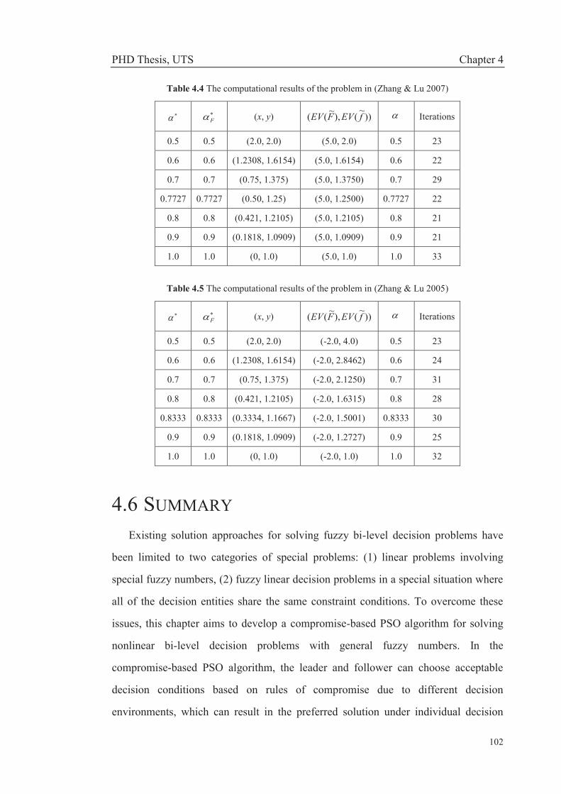
PHD Thesis, UTS Chapter 4
102
Table 4.4 The computational results of the problem in (Zhang & Lu 2007)
F (x, y) ))~
(),~(( fEVFEV Iterations
0.5 0.5 (2.0, 2.0) (5.0, 2.0) 0.5 23
0.6 0.6 (1.2308, 1.6154) (5.0, 1.6154) 0.6 22
0.7 0.7 (0.75, 1.375) (5.0, 1.3750) 0.7 29
0.7727 0.7727 (0.50, 1.25) (5.0, 1.2500) 0.7727 22
0.8 0.8 (0.421, 1.2105) (5.0, 1.2105) 0.8 21
0.9 0.9 (0.1818, 1.0909) (5.0, 1.0909) 0.9 21
1.0 1.0 (0, 1.0) (5.0, 1.0) 1.0 33
Table 4.5 The computational results of the problem in (Zhang & Lu 2005)
F (x, y) ))~
(),~(( fEVFEV Iterations
0.5 0.5 (2.0, 2.0) (-2.0, 4.0) 0.5 23
0.6 0.6 (1.2308, 1.6154) (-2.0, 2.8462) 0.6 24
0.7 0.7 (0.75, 1.375) (-2.0, 2.1250) 0.7 31
0.8 0.8 (0.421, 1.2105) (-2.0, 1.6315) 0.8 28
0.8333 0.8333 (0.3334, 1.1667) (-2.0, 1.5001) 0.8333 30
0.9 0.9 (0.1818, 1.0909) (-2.0, 1.2727) 0.9 25
1.0 1.0 (0, 1.0) (-2.0, 1.0) 1.0 32
4.6 SUMMARY Existing solution approaches for solving fuzzy bi-level decision problems have
been limited to two categories of special problems: (1) linear problems involving
special fuzzy numbers, (2) fuzzy linear decision problems in a special situation where
all of the decision entities share the same constraint conditions. To overcome these
issues, this chapter aims to develop a compromise-based PSO algorithm for solving
nonlinear bi-level decision problems with general fuzzy numbers. In the
compromise-based PSO algorithm, the leader and follower can choose acceptable
decision conditions based on rules of compromise due to different decision
environments, which can result in the preferred solution under individual decision
PHD Thesis, UTS Chapter 4
103
situations. To illustrate the effectiveness of the proposed compromise-based PSO
algorithm, the algorithm is applied to solve an illustrative example and two
benchmark examples. The computational results show that, the compromise-based
PSO algorithm can provide not only better solutions under the specific decision
situation compared with the existing solution approaches but also different options of
solutions due to various decision environments. In conclusion, the compromise-based
PSO algorithm provides an effective approach for solving fuzzy nonlinear bi-level
decision problems with general fuzzy numbers.

PHD Thesis, UTS Chapter 5
104
CHAPTER 5 TRI-LEVEL
MULTI-FOLLOWER DECISION
MAKING
5.1 INTRODUCTION With respect to a tri-level decision problem, multiple decision entities are often
involved at the middle and bottom levels; these entities are called multiple followers.
For example, in the tri-level decision-making case presented in Chapter 1, the sales
company (the leader) may have several subordinate logistics centers (the middle-level
followers) and there may also be several manufacturing factories (the bottom-level
followers) attached to each logistics center. Moreover, multiple followers at the same
level may have a variety of relationships with one another, which will generate
different decision processes.
In general, there are two fundamental issues in supporting this category of tri-level
multi-follower (TLMF) decision problems. One is how to use a model to describe the
decision-making process, which may manifest different characteristics at the three
decision levels, and the other is how to find an optimal solution to the problem. In
addition, the optimal solution means a compromised result for a TLMF decision
problem, which cannot completely reflect the operations of the complex TLMF
decision-making process; that is, it is imprecise or ambiguous for decision entities to
evaluate the solution obtained whether or not they desire to in real-world cases. It is
necessary to find a practical way to identify the satisfaction of decision entities
towards the solution obtained. However, existing tri-level decision-making research
PHD Thesis, UTS Chapter 5
105
has been primarily limited to a specific situation in which one single decision entity is
involved at each level.
To handle TLMF decision problems, this chapter first introduces various
relationships between multiple followers, gives linear TLMF decision models in line
with different relationships, and discusses theoretical properties in relation to the
existence and optimality of solutions. A TLMF Kth-Best algorithm is then developed
to find an optimal solution to TLMF decision models. An evaluation method based on
fuzzy programming is used to assess the satisfaction of decision entities towards the
obtained solution. Lastly, a detailed case study on production-inventory planning
illustrates the proposed TLMF decision-making techniques in applications.
This chapter is organized as follows. Following the introduction, general linear
TLMF decision models and related theoretical properties are proposed in Section 5.2.
In Section 5.3, the TLMF Kth-Best algorithm is developed. Section 5.4 presents the
solution evaluation method based on fuzzy programming. In Section 5.5, the proposed
TLMF decision-making techniques are applied to handle the real-world problem in
relation to production-inventory planning. A summary is given in Section 5.6.
5.2 TLMF DECISION MODELS AND RELATED
THEORETICAL PROPERTIES This section introduces definitions of three basic relationships (known as
uncooperative, cooperative and reference-based relationships) and their hybrid
relationships to describe a variety of decision-making situations between multiple
followers. In line with different relationships, TLMF decision models and their
solution concepts are given. Moreover, related theoretical properties are discussed,
which provide the theoretical basis for designing a solution algorithm.

PHD Thesis, UTS Chapter 5
106
5.2.1 TLMF DECISION MODELS AND SOLUTION
CONCEPTS
The organizational structure of the TLMF decision-making hierarchy is shown as
Figure 5.1. In this organizational structure, there are one leader, n middle-level
followers and im bottom-level followers attached to the middle-level follower i
( ni ,,2,1 ). Different TLMF decision models based on uncooperative, cooperative
and reference-based relationships are respectively defined as follows.
Leader
Middle-levelfollower 1
Middle-levelfollower n
Bottom-levelfollower 11
Bottom-levelfollower
Bottom-levelfollower n1
Bottom-levelfollower11m nnm
Figure 5.1 The organizational structure of the TLMF decision-making hierarchy
5.2.1.1 UNCOOPERATIVE TLMF DECISION MODEL
Multiple followers at the same level make their respective decisions
independently without any information exchange or share; this is known as an
uncooperative relationship between multiple followers at the same level. For example,
in the tri-level decision-making case given in Chapter 1 and Section 5.1, if logistics
centers and manufacturing factories make their respective and individual inventory or
production decisions without any information exchange or share, this can be called an
uncooperative relationship between the middle-level followers, as well as the
bottom-level followers.
Let kRXx , ikii RYy , ijk
ijij RZz denote the vectors of decision
variables of the leader, the middle-level follower i, and the bottom-level follower ij

PHD Thesis, UTS Chapter 5
107
respectively where nimj i ,,2,1,,,2,1 . Detailed definitions of the uncooperative
relationship are given as follows.
Definition 5.1 (Lu et al. 2012) Apart from the decision variables x and iimi zz ,,1
respectively controlled by the leader and bottom-level followers, if both the objective
function and constraint conditions of the middle-level follower i only involve its own
decision variable yi, this is known as the uncooperative relationship between the
middle-level follower i and other middle-level followers.
Definition 5.2 (Lu et al. 2012) Apart from the decision variables x and yi
respectively controlled by the leader and middle-level follower i, if both the objective
function and constraint conditions of the bottom-level follower ij only involve its own
decision variable zij, this is known as the uncooperative relationship between the
bottom-level follower ij and other bottom-level followers attached to the middle-level
follower i.
Based on Definitions 5.1 and 5.2, for kRXx , ikii RYy , ijk
ijij RZz ,
11111
)1(1
: RZZZYYXfnnmmn , 1
1)2( : RZZYXf
iimiii ,
1)3( : RZYXf ijiij , imj ,,2,1 , ni ,,2,1 , a linear TLMF decision model in
which the uncooperative relationship is involved at both middle and bottom levels is
defined as follows:
n
i
m
jijij
n
iiinmnmnXx
i
nzeydcxzzzzyyxf
1 1111111
)1( ),,,,,,,,,,(min1
(Leader) (5.1a)
s.t. ,1 11
bzCyBAxn
i
m
jijij
n
iii
i (5.1b)
where ),,,( 1 iimii zzy ),,2,1( ni , for each given x, solves (5.1c-5.1f):
i
iii
m
jijijiiiimiiiYy
zhygxczzyxf1
1)2( ),,,,(min (Middle-level follower i) (5.1c)

PHD Thesis, UTS Chapter 5
108
s.t. ,1
i
m
jijijiii bzEyDxA
i (5.1d)
where ijz ),,2,1( imj , for each given (x, yi), solves (5.1e-5.1f):
ijijiijijijiijZzzqypxczyxf
ijij
),,(min )3( (Bottom-level follower ij) (5.1e)
s.t. ,ijijijiijij bzQyPxA (5.1f)
where kiji Rccc ,, , ik
ijii Rpgd ,, , ijkijijij Rqhe ,, , ksRA , ks
iiRA , ks
ijijRA ,
iksi RB , ii ks
i RD , iij ksij RP , ijks
ij RC , iji ksij RE , ijij ks
ij RQ , sRb ,
isi Rb , ijs
ij Rb are matrices of decision coefficients.
To find an optimal solution to the TLMF decision model (5.1), solution concepts
in relation to operations of the uncooperative TLMF decision-making process are
presented as follows:
Definition 5.3
(1) Constraint region of the TLMF decision model (5.1):
:),,,,,,,,,,{(1 11
11111 1
n
i
m
jij
n
iinmnmn
i
nZYXzzzzyyxS
,,,11 1 1
ijijijiijiji
m
jijijiii
n
i
n
i
m
jijijii bzQyPxAbzEyDxAbzCyBAx
ii
imj ,,2,1 , ni ,,2,1 }.
(2) For each x given by the leader, feasible set of the middle-level follower i
),,2,1( ni and its bottom-level followers:
,:),,,{()(11
1 i
m
jijijiii
m
jijiimiii bzEyDxAZYzzyxS
ii
i
ijijijiijij bzQyPxA , },,2,1 imj .

PHD Thesis, UTS Chapter 5
109
(3) For each (x, yi) given by the leader and the middle-level follower i, feasible
set of the bottom-level follower ij ),,2,1,,,2,1( nimj i :
}:{),( ijijijiijijijijiij bzQyPxAZzyxS .
(4) For each (x, yi) given by the leader and the middle-level follower i, rational
reaction set of the bottom-level follower ij ( nimj i ,,2,1,,,2,1 ):
)]},(ˆ:)ˆ,,(min[arg:{),( )3(iijijijiijijijijiij yxSzzyxfzZzyxP .
(5) For each x given by the leader, rational reaction set of the middle-level
follower i ( ni ,,2,1 ) and its bottom-level followers:
,ˆ,(min[arg),,,(:),,,{()( )2(1
11 iiimii
m
jijiimiii yxfzzyZYzzyxP
i
i
i
]},,2,1),ˆ,(ˆ),()ˆ,,ˆ,ˆ(:)ˆ,,ˆ 11 iiijijiimiiimi mjyxPzxSzzyzzii
.
(6) Inducible region (IR) of model (5.1):
,,,,(:),,,,,,,,,,{( 11111 11 nnmnmmn yyxzzzzyyxIRn
},,2,1),(),,,(,),,,,,, 1111 11nixPzzySzzzz iimiinmnmm in
.
(7) Optimal solution set of model (5.1):
,,,,,,,,(:),,,,,,,,,,{(111 11111111 mnnmnmmn zzyyxzzzzyyxOS
n
]}),,,,,,,,,,(:min[arg),,111 1111
)1( IRzzzzyyxfzznn nmnmmnnmnm .
5.2.1.2 COOPERATIVE TLMF DECISION MODEL
Multiple followers at the same level share information and make joint decisions
because of common business needs; this is known as a cooperative relationship
between multiple followers at the same level. For example, in the tri-level
decision-making case given in Chapter 1 and Section 5.1, if the logistics centers share
a warehouse, they need to cooperate with each other for making an inventory solution

PHD Thesis, UTS Chapter 5
110
satisfied by every logistics center; this can be called a cooperative relationship
between the middle-level followers.
Let kRXx , iki RYy , ijk
iji RZz denote the vectors of decision variables
of the leader, the middle-level follower i, and the bottom-level follower ij respectively
where nimj i ,,2,1,,,2,1 . Detailed definitions of the cooperative relationship are
given as follows.
Definition 5.4 (Lu et al. 2012) Apart from the decision variables x and zi
respectively controlled by the leader and bottom-level followers, if both the objective
function and constraint conditions of the middle-level follower i involve the decision
variable y shared with other middle-level followers, this is known as the cooperative
relationship between the middle-level follower i and other middle-level followers.
Definition 5.5 (Lu et al. 2012) Apart from the decision variables x and y
respectively controlled by the leader and the middle-level follower i, if both the
objective function and constraint conditions of the bottom-level follower ij involve
the decision variable zi shared with other bottom-level followers attached to the
middle-level follower i, this is known as the cooperative relationship between the
bottom-level follower ij and other bottom-level followers attached to the middle-level
follower i.
Based on Definitions 5.4 and 5.5, for kRXx , iki RYy , nYYY 1 ,
0kRYy , ijkiji RZz ,
iimii ZZZ 1 , 0ikii RZz , 1)1( : RZZYXf ni ,
1)2( : RZYXf iii , 1)3( : RZYXf ijiij , imj ,,2,1 , ni ,,2,1 , a linear
TLMF decision model in which the cooperative relationship is involved at both
middle and bottom levels is defined as follows:
n
iiinXx
zedycxzzyxf1
1)1( ),,,,(min (Leader) (5.2a)
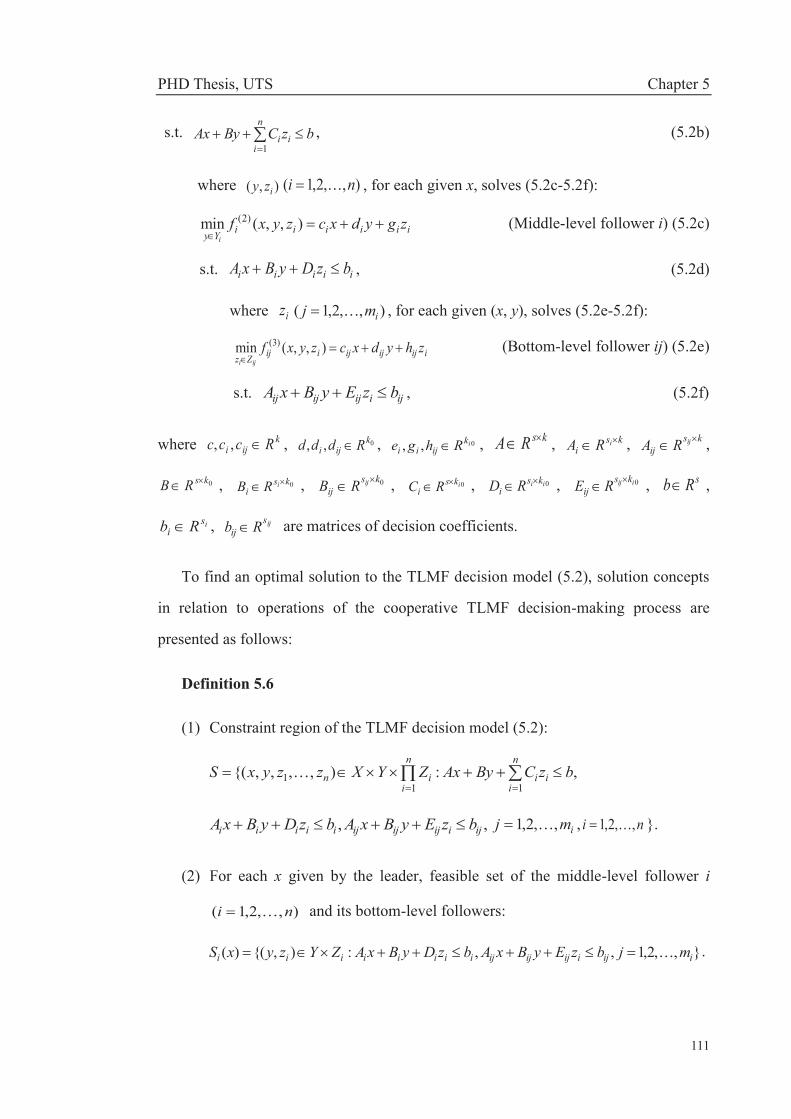
PHD Thesis, UTS Chapter 5
111
s.t. bzCByAxn
iii
1, (5.2b)
where ),( izy ),,2,1( ni , for each given x, solves (5.2c-5.2f):
iiiiiiYyzgydxczyxf
i
),,(min )2( (Middle-level follower i) (5.2c)
s.t. iiiii bzDyBxA , (5.2d)
where iz ),,2,1( imj , for each given (x, y), solves (5.2e-5.2f):
iijijijiijZzzhydxczyxf
iji
),,(min )3( (Bottom-level follower ij) (5.2e)
s.t. ijiijijij bzEyBxA , (5.2f)
where kiji Rccc ,, , 0,, k
iji Rddd , 0,, ikijii Rhge , ksRA , ks
iiRA , ks
ijijRA ,
0ksRB , 0ksi
iRB , 0ksij
ijRB , 0iksi RC , 0ii ks
i RD , 0iij ksij RE , sRb ,
isi Rb , ijs
ij Rb are matrices of decision coefficients.
To find an optimal solution to the TLMF decision model (5.2), solution concepts
in relation to operations of the cooperative TLMF decision-making process are
presented as follows:
Definition 5.6
(1) Constraint region of the TLMF decision model (5.2):
,:),,,,{(11
1 bzCByAxZYXzzyxSn
iii
n
iin
,, ijiijijijiiiii bzEyBxAbzDyBxA imj ,,2,1 , ni ,,2,1 }.
(2) For each x given by the leader, feasible set of the middle-level follower i
),,2,1( ni and its bottom-level followers:
},,2,1,,:),{()( iijiijijijiiiiiiii mjbzEyBxAbzDyBxAZYzyxS .
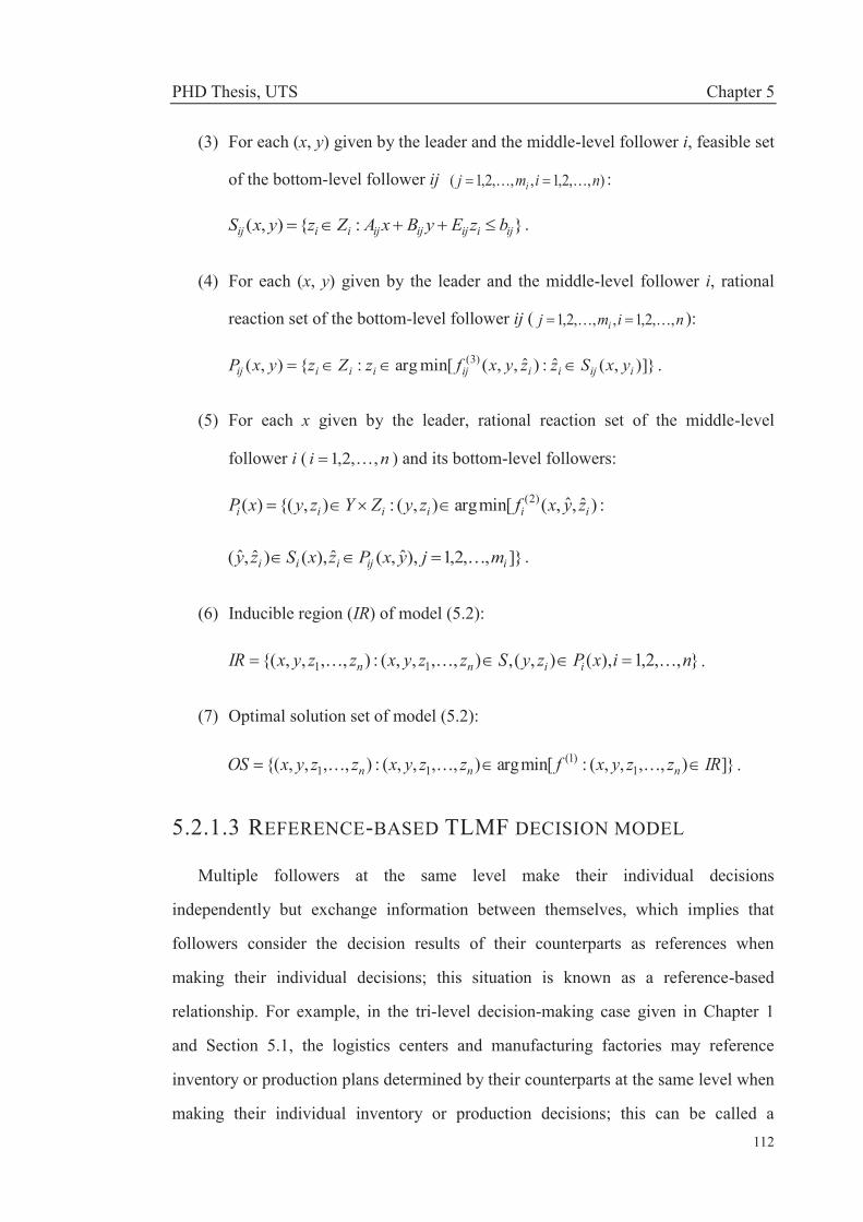
PHD Thesis, UTS Chapter 5
112
(3) For each (x, y) given by the leader and the middle-level follower i, feasible set
of the bottom-level follower ij ),,2,1,,,2,1( nimj i :
}:{),( ijiijijijiiij bzEyBxAZzyxS .
(4) For each (x, y) given by the leader and the middle-level follower i, rational
reaction set of the bottom-level follower ij ( nimj i ,,2,1,,,2,1 ):
)]},(ˆ:)ˆ,,(min[arg:{),( )3(iijiiijiiiij yxSzzyxfzZzyxP .
(5) For each x given by the leader, rational reaction set of the middle-level
follower i ( ni ,,2,1 ) and its bottom-level followers:
:)ˆ,ˆ,(min[arg),(:),{()( )2(iiiiii zyxfzyZYzyxP
]},,2,1),ˆ,(ˆ),()ˆ,ˆ( iijiii mjyxPzxSzy .
(6) Inducible region (IR) of model (5.2):
},,2,1),(),(,),,,,(:),,,,{( 11 nixPzySzzyxzzyxIR iinn .
(7) Optimal solution set of model (5.2):
]}),,,,(:min[arg),,,,(:),,,,{( 1)1(
11 IRzzyxfzzyxzzyxOS nnn .
5.2.1.3 REFERENCE-BASED TLMF DECISION MODEL
Multiple followers at the same level make their individual decisions
independently but exchange information between themselves, which implies that
followers consider the decision results of their counterparts as references when
making their individual decisions; this situation is known as a reference-based
relationship. For example, in the tri-level decision-making case given in Chapter 1
and Section 5.1, the logistics centers and manufacturing factories may reference
inventory or production plans determined by their counterparts at the same level when
making their individual inventory or production decisions; this can be called a

PHD Thesis, UTS Chapter 5
113
reference-based relationship between the middle-level followers, as well as the
bottom-level followers.
Let kRXx , ikii RYy , ijk
ijij RZz denote the vectors of decision
variables of the leader, the middle-level follower i, and the bottom-level follower ij
respectively where imj ,,2,1 , ni ,,2,1 . Detailed definitions of the
reference-based relationship are given as follows.
Definition 5.7 (Lu et al. 2012) Apart from its own decision variable iy and the
decision variables iimi zzx ,,, 1 determined by the leader and the bottom-level
followers, if both the objective function and constraint conditions of the middle-level
follower i involve the decision variables nii yyyy ,,,,, 111 controlled by other
middle-level followers, this is known as the reference-based relationship between the
middle-level follower i and other middle-level followers.
Definition 5.8 (Lu et al. 2012) Apart from its own decision variable ijz and the
decision variables x and iy respectively determined by the leader and the
middle-level follower i, if both the objective function and constraint conditions of the
bottom-level follower ij involve the decision variables iimjijii zzzz ,,,,, )1()1(1
controlled other bottom-level followers attached to the same middle-level follower i,
this is known as the reference-based relationship between the bottom-level follower ij
and other bottom-level followers attached to the middle-level follower i.
Based on Definitions 5.7 and 5.8, for kRXx , ikii RYy , ijk
ijij RZz ,
11111
)1(1
: RZZZYYXfnnmmn , 1
11)2( : RZZYYXf
iimini ,
11
)3( : RZZYXfiimiiij , imj ,,2,1 , ni ,,2,1 , a linear TLMF decision
model in which the reference-based relationship is involved at both middle and
bottom levels is defined as follows:
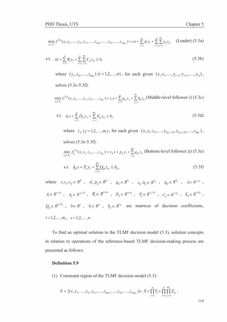
PHD Thesis, UTS Chapter 5
114
n
i
m
jijij
n
iiinmnmnXx
i
nzeydcxzzzzyyxf
1 1111111
)1( ),,,,,,,,,,(min1
(Leader) (5.3a)
s.t. ,1 11
bzCyBAxn
i
m
jijij
n
iii
i (5.3b)
where ),,,( 1 iimii zzy ),,2,1( ni , for each given ),,,,,,( 111 nii yyyyx ,
solves (5.3c-5.3f):
i
iii
m
jijij
n
ssisiiminiYy
zhygxczzyyxf11
11)2( ),,,,,,(min (Middle-level follower i) (5.3c)
s.t. ,11
i
m
jijij
n
ssisi bzEyDxA
i (5.3d)
where ijz ),,2,1( imj , for each given ),,,,,,,( )1()1(1 iimjijiii zzzzyx ,
solves (5.3e-5.3f): i
iijij
m
titijtiijijimiiijZz
zqypxczzyxf1
1)3( ),,,,(min (Bottom-level follower ij) (5.3e)
s.t. ,1
ij
m
titijtiijij bzQyPxA
i (5.3f)
where kiji Rccc ,, , ik
iji Rpd , , skis Rg , ijk
ijij Rhe , , itkijt Rq , krRA ,
kri
iRA , krij
ijRA , ikri RB , si kr
is RD , iij krij RP , ijkr
ij RC , iji krij RE ,
itij krijt RQ , rRb , ir
i Rb , ijrij Rb are matrices of decision coefficients,
imt ,,2,1 , ns ,,2,1 .
To find an optimal solution to the TLMF decision model (5.3), solution concepts
in relation to operations of the reference-based TLMF decision-making process are
presented as follows:
Definition 5.9
(1) Constraint region of the TLMF decision model (5.3):
:),,,,,,,,,,{(1 11
11111 1
n
i
m
jij
n
iinmnmn
i
nZYXzzzzyyxS

PHD Thesis, UTS Chapter 5
115
,,111 1 1
i
m
jijij
n
ssisi
n
i
n
i
m
jijijii bzEyDxAbzCyBAx
ii
iij
m
titijtiijij mjbzQyPxA
i
,,2,1,1
, ni ,,2,1 }.
(2) For each ),,,,,,( 111 nii yyyyx given by the leader and other
middle-level followers, feasible set of the middle-level follower i
),,2,1( ni and its bottom-level followers:
:),,,{(),,,,,,(1
1111i
i
m
jijiimiiniii ZYzzyyyyyxS
},,2,1,,111
iij
m
titijtiijiji
m
jijij
n
ssisi mjbzQyPxAbzEyDxA
ii.
(3) For each ),,,,,,,( )1()1(1 iimjijiii zzzzyx given by the leader, the
middle-level follower i and bottom-level followers, feasible set of the
bottom-level follower ij ),,2,1,,,2,1( nimj i :
}:{),,,,,,,(1
)1()1(1 ij
m
titijtiijijijijimjijiiiij bzQyPxAZzzzzzyxS
i
i.
(4) For each ),,,,,,,( )1()1(1 iimjijiii zzzzyx given by the leader, the
middle-level follower i and bottom-level followers, rational reaction set of the
bottom-level follower ij ( nimj i ,,2,1,,,2,1 ):
:{),,,,,,,( )1()1(1 ijijimjijiiiij ZzzzzzyxPi
),,,,ˆ,,,,,(min[arg )1()1(1)3(
iimjiijjiiiijij zzzzzyxfz
)]},,,,,,,(ˆ )1()1(1 iimjijiiiijij zzzzyxSz .
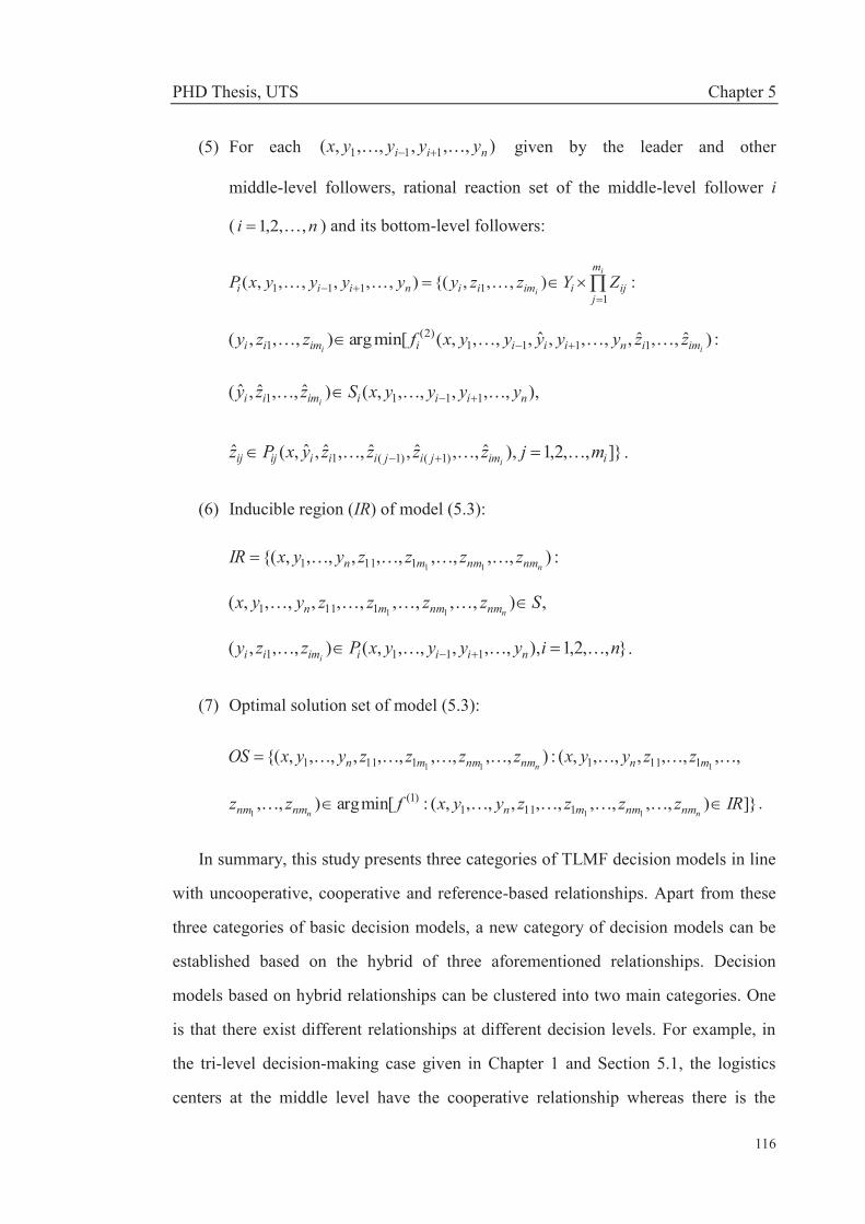
PHD Thesis, UTS Chapter 5
116
(5) For each ),,,,,,( 111 nii yyyyx given by the leader and other
middle-level followers, rational reaction set of the middle-level follower i
( ni ,,2,1 ) and its bottom-level followers:
:),,,{(),,,,,,(1
1111i
i
m
jijiimiiniii ZYzzyyyyyxP
:)ˆ,,ˆ,,,,ˆ,,,,(min[arg),,,( 1111)2(
1 ii iminiiiiimii zzyyyyyxfzzy
),,,,,,,()ˆ,,ˆ,ˆ( 1111 niiiimii yyyyxSzzyi
]},,2,1),ˆ,,ˆ,ˆ,,ˆ,ˆ,(ˆ )1()1(1 iimjijiiiijij mjzzzzyxPzi
.
(6) Inducible region (IR) of model (5.3):
:),,,,,,,,,,{(111111 nnmnmmn zzzzyyxIR
,),,,,,,,,,,(111111 Szzzzyyx
nnmnmmn
},,2,1),,,,,,,(),,,( 1111 niyyyyxPzzy niiiimii i.
(7) Optimal solution set of model (5.3):
,,,,,,,,(:),,,,,,,,,,{(111 11111111 mnnmnmmn zzyyxzzzzyyxOS
n
]}),,,,,,,,,,(:min[arg),,111 1111
)1( IRzzzzyyxfzznn nmnmmnnmnm .
In summary, this study presents three categories of TLMF decision models in line
with uncooperative, cooperative and reference-based relationships. Apart from these
three categories of basic decision models, a new category of decision models can be
established based on the hybrid of three aforementioned relationships. Decision
models based on hybrid relationships can be clustered into two main categories. One
is that there exist different relationships at different decision levels. For example, in
the tri-level decision-making case given in Chapter 1 and Section 5.1, the logistics
centers at the middle level have the cooperative relationship whereas there is the
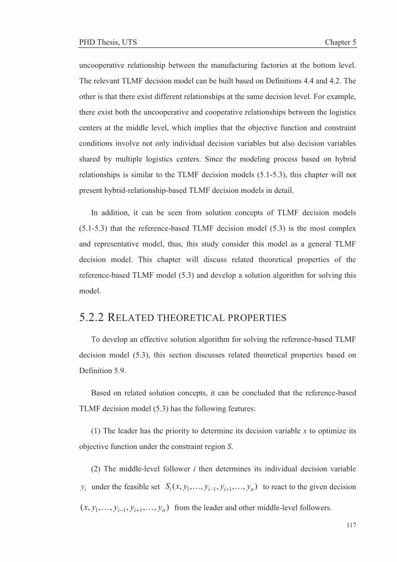
PHD Thesis, UTS Chapter 5
117
uncooperative relationship between the manufacturing factories at the bottom level.
The relevant TLMF decision model can be built based on Definitions 4.4 and 4.2. The
other is that there exist different relationships at the same decision level. For example,
there exist both the uncooperative and cooperative relationships between the logistics
centers at the middle level, which implies that the objective function and constraint
conditions involve not only individual decision variables but also decision variables
shared by multiple logistics centers. Since the modeling process based on hybrid
relationships is similar to the TLMF decision models (5.1-5.3), this chapter will not
present hybrid-relationship-based TLMF decision models in detail.
In addition, it can be seen from solution concepts of TLMF decision models
(5.1-5.3) that the reference-based TLMF decision model (5.3) is the most complex
and representative model, thus, this study consider this model as a general TLMF
decision model. This chapter will discuss related theoretical properties of the
reference-based TLMF model (5.3) and develop a solution algorithm for solving this
model.
5.2.2 RELATED THEORETICAL PROPERTIES
To develop an effective solution algorithm for solving the reference-based TLMF
decision model (5.3), this section discusses related theoretical properties based on
Definition 5.9.
Based on related solution concepts, it can be concluded that the reference-based
TLMF decision model (5.3) has the following features:
(1) The leader has the priority to determine its decision variable x to optimize its
objective function under the constraint region S.
(2) The middle-level follower i then determines its individual decision variable
iy under the feasible set ),,,,,,( 111 niii yyyyxS to react to the given decision
),,,,,,( 111 nii yyyyx from the leader and other middle-level followers.
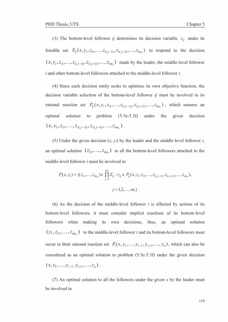
PHD Thesis, UTS Chapter 5
118
(3) The bottom-level follower ij determines its decision variable ijz under its
feasible set ),,,,,,,( )1()1(1 iimjijiiiij zzzzyxS to respond to the decision
),,,,,,,( )1()1(1 iimjijiii zzzzyx made by the leader, the middle-level follower
i and other bottom-level followers attached to the middle-level follower i.
(4) Since each decision entity seeks to optimize its own objective function, the
decision variable selection of the bottom-level follower ij must be involved in its
rational reaction set ),,,,,,,( )1()1(1 iimjijiiiij zzzzyxP , which ensures an
optimal solution to problem (5.3e-5.3f) under the given decision
),,,,,,,( )1()1(1 iimjijiii zzzzyx .
(5) Under the given decision (x, yi) by the leader and the middle-level follower i,
an optimal solution ),,( 1 iimi zz to all the bottom-level followers attached to the
middle-level follower i must be involved in
),,,,,,,,(:),,{(),( )1()1(11
1 i
i
i imjijiiiijij
m
jijimiii zzzzyxPzZzzyxP
},,2,1 imj .
(6) As the decision of the middle-level follower i is affected by actions of its
bottom-level followers, it must consider implicit reactions of its bottom-level
followers when making its own decisions, thus, an optimal solution
),,,( 1 iimii zzy to the middle-level follower i and its bottom-level followers must
occur in their rational reaction set ),,,,,,( 111 niii yyyyxP , which can also be
considered as an optimal solution to problem (5.3c-5.3f) under the given decision
),,,,,,( 111 nii yyyyx .
(7) An optimal solution to all the followers under the given x by the leader must
be involved in

PHD Thesis, UTS Chapter 5
119
),,,,,,,(),,,(:),,,,,,,,,{()( 111111111 1 niiiimiinmnmn yyyyxPzzyzzzzyyxPin
},,2,1 ni .
(8) As the leader should consider implicit reactions of all the followers when
making its own decisions, an optimal solution to model (5.3) must occur over the IR
and the optimal solution set is expressed by OS.
To ensure that the model (5.3) is well posed, it is necessary to make the following
assumptions as the basis for the existence of solutions.
Assumption 5.1 S is nonempty and compact.
Assumption 5.2 IR is nonempty.
Assumption 5.3 ),( ii yxP and )(xP have at most one solution respectively for
each parameter ),( iyx and x, where ni ,,2,1 .
Theorem 5.1 If the above Assumptions 5.1-5.3 hold, there exists an optimal
solution to the TLMF decision model (5.3).
Proof. Since both S and IR are not empty, there is at least one parameter value x
and )(xP . Consider a sequence ,,,,,,,,,,{( 11111 1
tn
tm
ttn
tt zzzyyx
IRz ttnmn 1)} converging to ,,,,,,,,(
11111 mn zzyyx ),,1 nnmn zz . Then,
since )(),,,,,,,,,( 11111 1
ttnm
tn
tm
ttn
t xPzzzzyyn
, let ,,,,,()( 1110tt
ntt zyyxP
),,,, 11 1
tnm
tn
tm n
zzz and )()(0tt xPxP . Because of the continuity properties of
linear parametric optimization proposed in (Dempe 2002) and *lim xxt
t,
)()(lim *00 xPxP t
t is obtained. Since ),,,,,,,,,()(lim 111110 1 nnmnmn
t
tzzzzyyxP
and )()( **0 xPxP , )(),,,,,,,,,( 11111 1
xPzzzzyynnmnmn . Hence, IR is
closed. Also, IR is bounded by SIR and Assumption 5.1. Therefore, the inducible
region IR is a nonempty and compact set. Furthermore, by Assumption 5.3, the

PHD Thesis, UTS Chapter 5
120
solution ),,( 1 iimi zz to the bottom-level followers attached to the middle-level
follower i ( ni ,,2,1 ) and the solution ),,,,,,,,,( 11111 1 nnmnmn zzzzyy to
all the followers are uniquely determined respectively for the given value ),( iyx
and x , which implies that the leader must optimize its objective over IR. According
to the optimal solution set OS in Definition 5.9, finding an optimal solution to model
(5.3) is equivalent to solving the following problem:
:),,,,,,,,,,(min{ 11111)1(
1 nnmnmn zzzzyyxf
}.),,,,,,,,,,( 11111 1IRzzzzyyx
nnmnmn (5.4)
Clearly, problem (5.4) consists of minimizing a continuous function over a nonempty
and compact set IR, which implies that there exists an optimal solution to the problem
(5.4) that is also an optimal solution to the TLMF decision model (5.3). □
It is noticeable from the Theorem 2.1 that if the followers have multiple optimal
solutions to respond to the parameter value x of the leader, it will be difficult for the
leader to realize its objective function value prior to the determination of the optimal
solution taken by the followers (Mersha & Dempe 2006). In this case, if the followers
cannot select the solution preferred by the leader, the leader may achieve its optimal
solution outside IR, which implies that the TLMF decision model (5.3) may not have
an optimal solution. Therefore, to avoid this situation in the presentation of solution
algorithms, the Assumption 5.3 is necessary.
Theorem 5.2 The IR can be expressed equivalently as a piecewise linear equality
constraint comprised of supporting hyperplanes of S.
Proof. First, for nimj i ,,2,1,,,2,1 , define
),,,,,,,( )1()1(1 iimjijiiiij zzzzyxF
)},,,,,,,,(:min{ )1()1(1 iimjijiiiijijijijj zzzzyxSzzq
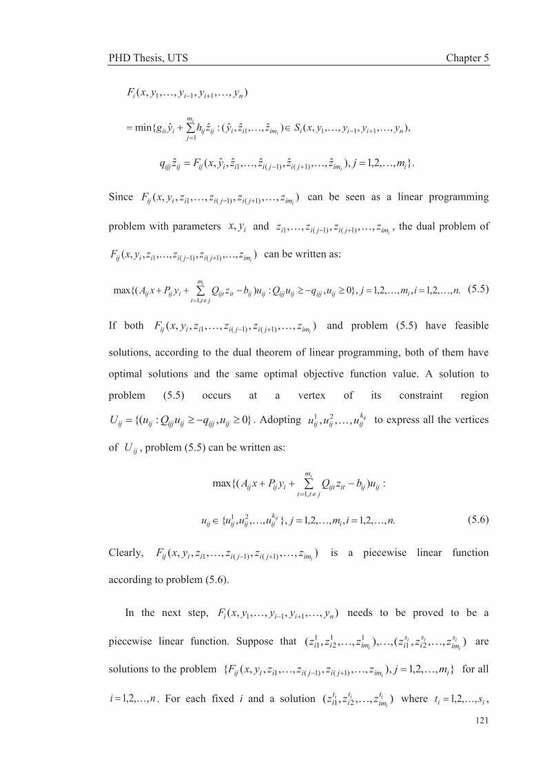
PHD Thesis, UTS Chapter 5
121
),,,,,,( 111 niii yyyyxF
),,,,,,,()ˆ,,ˆ,ˆ(:ˆˆmin{ 11111
niiiimii
m
jijijiii yyyyxSzzyzhyg
i
i
}.,,2,1),ˆ,,ˆ,ˆ,,ˆ,ˆ,(ˆ )1()1(1 iimjijiiiijijijj mjzzzzyxFzqi
Since ),,,,,,,( )1()1(1 iimjijiiiij zzzzyxF can be seen as a linear programming
problem with parameters iyx, and iimjijii zzzz ,,,,, )1()1(1 , the dual problem of
),,,,,,,( )1()1(1 iimjijiiiij zzzzyxF can be written as:
.,,2,1,,,2,1},0,:)max{(,1
nimjuquQubzQyPxA iijijjijijjijij
m
jttitijtiijij
i (5.5)
If both ),,,,,,,( )1()1(1 iimjijiiiij zzzzyxF and problem (5.5) have feasible
solutions, according to the dual theorem of linear programming, both of them have
optimal solutions and the same optimal objective function value. A solution to
problem (5.5) occurs at a vertex of its constraint region
}0,:{( ijijjijijjijij uquQuU . Adopting ijkijijij uuu ,,, 21 to express all the vertices
of ijU , problem (5.5) can be written as:
:)max{(,1
ijij
m
jttitijtiijij ubzQyPxA
i
.,,2,1,,,2,1},,,,{ 21 nimjuuuu ikijijijij
ij (5.6)
Clearly, ),,,,,,,( )1()1(1 iimjijiiiij zzzzyxF is a piecewise linear function
according to problem (5.6).
In the next step, ),,,,,,( 111 niii yyyyxF needs to be proved to be a
piecewise linear function. Suppose that ),,,(,),,,,( 2111
211
ii
iii
sim
si
siimii zzzzzz are
solutions to the problem },,2,1),,,,,,,,({ )1()1(1 iimjijiiiij mjzzzzyxFi
for all
ni ,,2,1 . For each fixed i and a solution ),,,( 21i
iii t
imti
ti zzz where ii st ,,2,1 ,
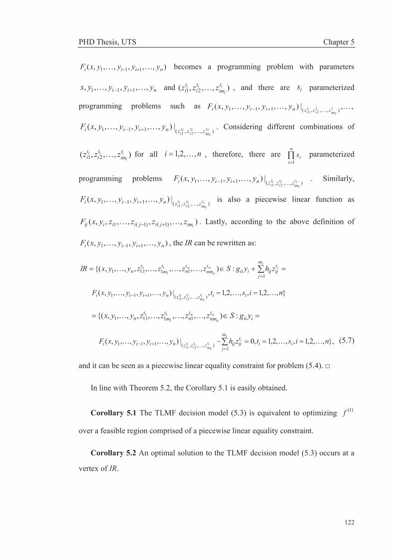
PHD Thesis, UTS Chapter 5
122
),,,,,,( 111 niii yyyyxF becomes a programming problem with parameters
nii yyyyx ,,,,,, 111 and ),,,( 21i
iii t
imti
ti zzz , and there are is parameterized
programming problems such as ,,|),,,,,,( ),,,(111 112
11 iimii zzzniii yyyyxF
),,,(11121
|),,,,,,( isiim
isi
isi zzzniii yyyyxF . Considering different combinations of
),,,( 21i
iii t
imti
ti zzz for all ni ,,2,1 , therefore, there are
n
iis
1 parameterized
programming problems ),,,(111
21|),,,,,,( it
iimit
iit
i zzzniii yyyyxF . Similarly,
),,,(11121
|),,,,,,( itiim
iti
iti zzzniii yyyyxF is also a piecewise linear function as
),,,,,,,( )1()1(1 iimjijiiiij zzzzyxF . Lastly, according to the above definition of
),,,,,,( 111 niii yyyyxF , the IR can be rewritten as:
iin
nn
m
j
tijijiii
tnm
tn
tm
tn zhygSzzzzyyxIR
111111 :),,,,,,,,,,{( 1
11
},,2,1,,,2,1,|),,,,,,(),,,(111
21nistyyyyxF iizzzniii it
iimit
iit
i
iiitnm
tn
tm
tn ygSzzzzyyx n
nn :),,,,,,,,,,{( 11111
11
1
},,,2,1,,,2,1,0|),,,,,,(1),,,(111
21nistzhyyyyxF ii
m
j
tijijzzzniii
ii
itiim
iti
iti
(5.7)
and it can be seen as a piecewise linear equality constraint for problem (5.4). □
In line with Theorem 5.2, the Corollary 5.1 is easily obtained.
Corollary 5.1 The TLMF decision model (5.3) is equivalent to optimizing )1(f
over a feasible region comprised of a piecewise linear equality constraint.
Corollary 5.2 An optimal solution to the TLMF decision model (5.3) occurs at a
vertex of IR.

PHD Thesis, UTS Chapter 5
123
Proof. According to the equivalent form (5.4) of the TLMF decision model (5.3)
and since ),,,,,,,,,,( 11111)1(
1 nnmnmn zzzzyyxf is linear, an optimal solution
to the problem must occur at a vertex of IR if it exists. □
Theorem 5.3 An optimal solution ),,,,,,,,,,( 11111 1 nnmnmn zzzzyyx to
the TLMF decision model (5.3) occurs at a vertex of S.
Proof. Let ),,,,,,,,,,(,),,,,,,,,,,,( 1111111
111
111
111
111
tnm
tn
tm
ttn
ttnmnmn nn
zzzzyyxzzzzyyx
express the distinct vertices of S. Since any point in S can be written as a convex
combination of these vertices, t
r
rnm
rn
rm
rrn
rrrnmnmn nn
zzzzyyxzzzzyyx1
1111111111 ),,,,,,,,,,(),,,,,,,,,,(11
is obtained, where t
rr
1,1 ,0r tr ,,2,1 and tt . By the convexity of
),,,,,,( 111 niii yyyyxF , let us write the constraints of model (5.3) in the
piecewise linear form (5.7) discussed in Theorem 5.2:
i
iimii
m
jijijiiizzzniii zhygyyyyxF
1),,,(111
21|),,,,,,(0
)(|)),,,,,,((111
),,,(1
11121
t
r
rijr
m
jij
t
r
ririizzz
t
r
rn
ri
ri
rrri zhygyyyyxF
i
iimii
)(|),,,,,,(111
),,,(1111 21
i
iimii
m
j
rijij
t
rr
t
r
riiirzzz
rn
ri
ri
rri
t
rr zhygyyyyxF
.,,2,1),|),,,,,,((1
),,,(1111 21
nizhygyyyyxFi
iimii
m
j
rijij
riiizzz
rn
ri
ri
rri
t
rr (5.8)
By the definition of ),,,(111
21|),,,,,,( is
iimis
iis
i zzzniii yyyyxF ,
),,,(11121
|),,,,,,(iimii zzz
rn
ri
ri
rri yyyyxF
.,,2,1,,,2,1,)min(11
nitrzhygzhygii
im
j
rijij
riii
m
j
tijijiii

PHD Thesis, UTS Chapter 5
124
Thus,
.,,2,1,,,2,1,0|),,,,,,(1
),,,(11121
nitrzhygyyyyxFi
iimii
m
j
rijij
riiizzz
rn
ri
ri
rri
Because the preceding expression (5.8) must be held with 0r , tr ,,2,1 , there
must exist ,,,2,1,0|),,,,,,(1
),,,(11121
trzhygyyyyxFi
iimii
m
j
rijij
riiizzz
rn
ri
ri
rri
ni ,,2,1 . These statements imply that ,),,,,,,,,,,( 11111 1IRzzzzyyx r
nmrn
rm
rrn
rrn
tr ,,2,1 , and that ),,,,,,,,,,( 11111 1 nnmnmn zzzzyyx can be denoted as a
convex combination of the points in the IR. Since
),,,,,,,,,,( 11111 1 nnmnmn zzzzyyx is a vertex of the IR according to Corollary 5.2,
there must exist 1t , which implies that ),,,,,,,,,,( 11111 1 nnmnmn zzzzyyx is a
vertex of S. □
Corollary 5.3 If ),,,,,,,,,,( 11111 1 nnmnmn zzzzyyx is a vertex of the IR,
it is also a vertex of S.
5.3 TLMF KTH-BEST ALGORITHM AND A
NUMERICAL EXAMPLE This section first presents the TLMF Kth-Best algorithm for solving the TLMF
decision model (5.3) based on related theoretical properties. A numerical example is
then used to illustrate how the TLMF Kth-Best algorithm works.
5.3.1 TLMF KTH-BEST ALGORITHM DESCRIPTION
Theorem 5.3 and Corollary 5.3 imply that an optimal solution to the TLMF
decision model (5.3) can be found by enumerating vertices (also called extreme points)
of the constraint region S, which clearly provide an appropriate way to develop the
following TLMF Kth-Best algorithm to solve the problem. According to the notations
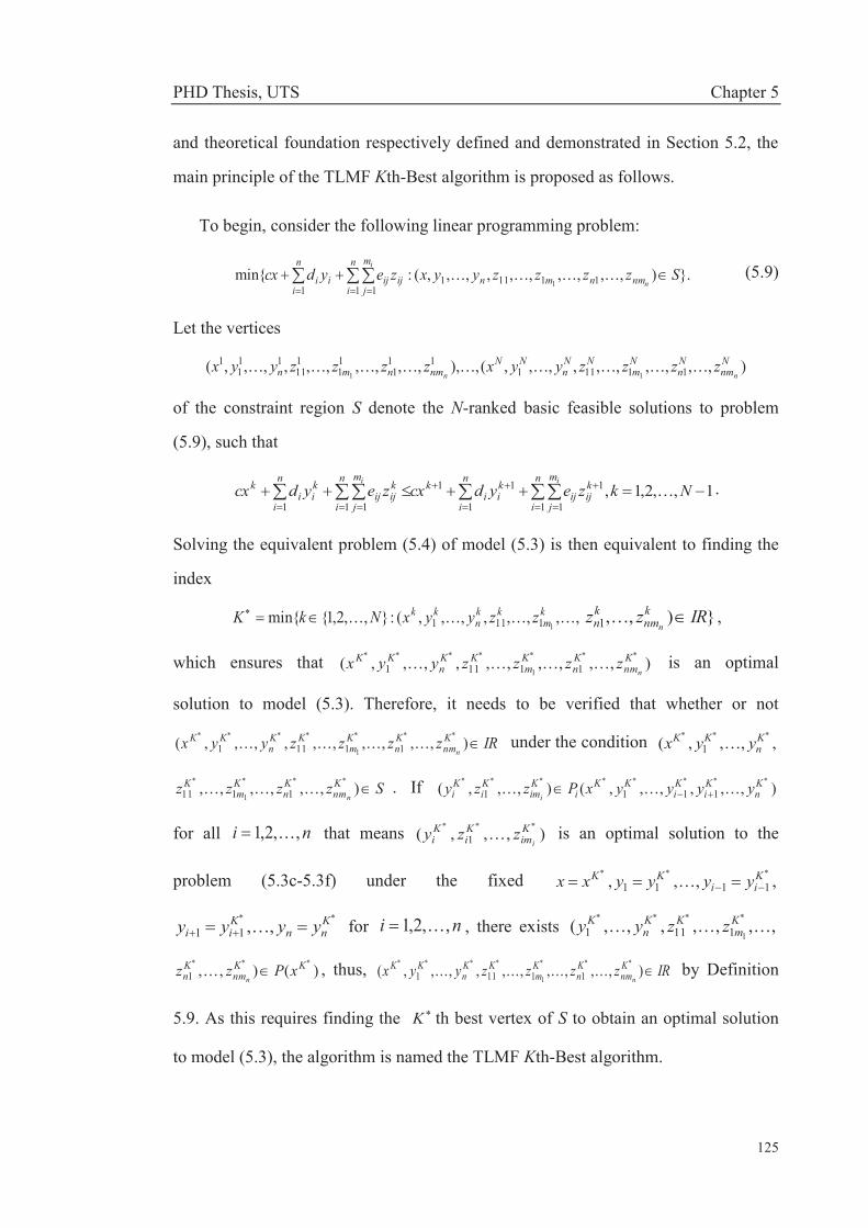
PHD Thesis, UTS Chapter 5
125
and theoretical foundation respectively defined and demonstrated in Section 5.2, the
main principle of the TLMF Kth-Best algorithm is proposed as follows.
To begin, consider the following linear programming problem:
}.),,,,,,,,,,(:min{ 111111 11
1Szzzzyyxzeydcx
n
i
nmnmn
n
i
m
jijij
n
iii (5.9)
Let the vertices
),,,,,,,,,,(,),,,,,,,,,,,( 1111111
111
111
111
111
Nnm
Nn
Nm
NNn
NNnmnmn nn
zzzzyyxzzzzyyx
of the constraint region S denote the N-ranked basic feasible solutions to problem
(5.9), such that
1,,2,1,1 1
1
1
11
1 11Nkzeydcxzeydcx
n
i
m
j
kijij
n
i
kii
kn
i
m
j
kijij
n
i
kii
k ii .
Solving the equivalent problem (5.4) of model (5.3) is then equivalent to finding the
index
,,,,,,,,(:},,2,1{min{11111
km
kkn
kk zzyyxNkK }),,1 IRzz knm
kn n
,
which ensures that ),,,,,,,,,,( 11111 1
Knm
Kn
Km
KKn
KKn
zzzzyyx is an optimal
solution to model (5.3). Therefore, it needs to be verified that whether or not
IRzzzzyyx Knm
Kn
Km
KKn
KKn),,,,,,,,,,( 11111 1
under the condition ,,,,( 1Kn
KK yyx
Szzzz Knm
Kn
Km
Kn),,,,,, 1111 1
. If ),,,,,,(),,,( 1111Kn
Ki
Ki
KKi
Kim
Ki
Ki yyyyxPzzy
i
for all ni ,,2,1 that means ),,,( 1Kim
Ki
Ki i
zzy is an optimal solution to the
problem (5.3c-5.3f) under the fixed ,,,, 1111Kii
KK yyyyxx
Knn
Kii yyyy ,,11 for ni ,,2,1 , there exists ,,,,,,,(
11111Km
KKn
K zzyy
)(),,1KK
nmKn xPzz
n, thus, IRzzzzyyx K
nmKn
Km
KKn
KKn),,,,,,,,,,( 11111 1
by Definition
5.9. As this requires finding the K th best vertex of S to obtain an optimal solution
to model (5.3), the algorithm is named the TLMF Kth-Best algorithm.
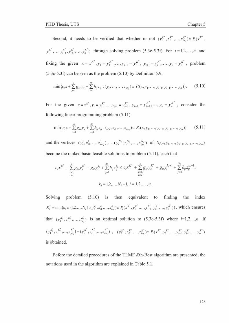
PHD Thesis, UTS Chapter 5
126
Second, it needs to be verified that whether or not ,(),,,( 1K
iKim
Ki
Ki xPzzy
i
),,,,, 111Kn
Ki
Ki
K yyyy through solving problem (5.3c-5.3f). For ni ,,2,1 and
fixing the given ,,,, 1111Kii
KK yyyyxx Knn
Kii yyyy ,,11 , problem
(5.3c-5.3f) can be seen as the problem (5.10) by Definition 5.9:
)}.,,,,,,(),,,(:min{ 111111
niiiimii
m
jijij
n
ssisi yyyyxPzzyzhygxc
i
i (5.10)
For the given ,,,, 1111Kii
KK yyyyxx Knn
Kii yyyy ,,11 , consider the
following linear programming problem (5.11):
)},,,,,,(),,,(:min{ 111111
niiiimii
m
jijij
n
ssisi yyyyxSzzyzhygxc
i
i (5.11)
and the vertices ),,,(,),,,,( 111
11 i
iii
i
Nim
Ni
Niimii zzyzzy of ),,,,,,( 111 niii yyyyxS
become the ranked basic feasible solutions to problem (5.11), such that
iii
m
j
kijij
kiii
n
iss
Ksis
Ki zhygygxc
1,1,
1
11
,1
iii
m
j
kijij
kiii
n
iss
Ksis
Ki zhygygxc
,1,,2,1 ii Nk ni ,,2,1 .
Solving problem (5.10) is then equivalent to finding the index
)},,,,,,(),,,(:},,2,1{min{ 1111Kn
Ki
Ki
KKi
kim
ki
kiiii yyyyxPzzyNkK i
iii , which ensures
that ),,,( 11ii
ii Kim
Ki
K zzy is an optimal solution to (5.3c-5.3f) where i=1,2,...,n. If
),,,(),,,( 111Kim
Ki
Ki
Kim
Ki
Ki
ii
ii zzyzzy , ),,,,,,(),,,( 1111Kn
Ki
Ki
KKi
Kim
Ki
Ki yyyyxPzzy
i
is obtained.
Before the detailed procedures of the TLMF Kth-Best algorithm are presented, the
notations used in the algorithm are explained in Table 5.1.
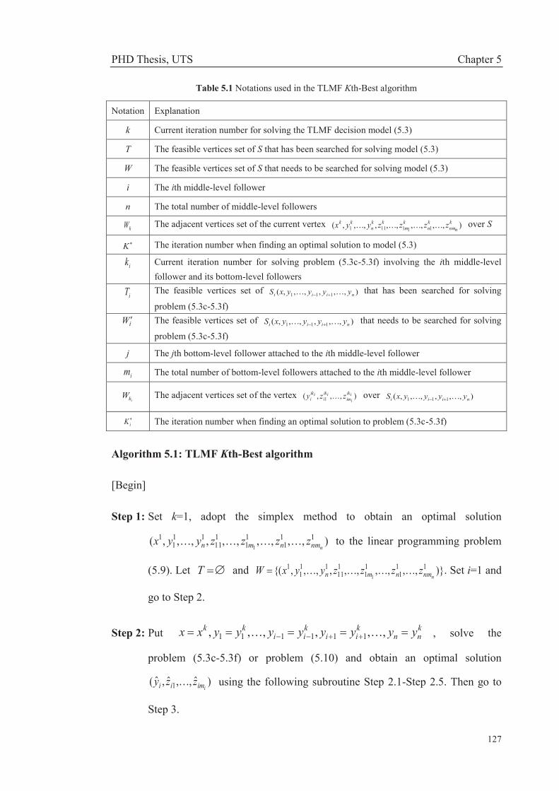
PHD Thesis, UTS Chapter 5
127
Table 5.1 Notations used in the TLMF Kth-Best algorithm
Notation Explanation
k Current iteration number for solving the TLMF decision model (5.3)
T The feasible vertices set of S that has been searched for solving model (5.3)
W The feasible vertices set of S that needs to be searched for solving model (5.3)
i The ith middle-level follower
n The total number of middle-level followers
kW The adjacent vertices set of the current vertex ),,,,,,,,,,( 111111k
nnmkn
km
kkn
kk zzzzyyx over S
K The iteration number when finding an optimal solution to model (5.3)
ik Current iteration number for solving problem (5.3c-5.3f) involving the ith middle-level follower and its bottom-level followers
iT The feasible vertices set of ),,,,,,( 111 niii yyyyxS that has been searched for solving
problem (5.3c-5.3f)
iW The feasible vertices set of ),,,,,,( 111 niii yyyyxS that needs to be searched for solving
problem (5.3c-5.3f)
j The jth bottom-level follower attached to the ith middle-level follower
im The total number of bottom-level followers attached to the ith middle-level follower
ikW The adjacent vertices set of the vertex ),,,( 1iikiim
iiki
iiki zzy over ),,,,,,( 111 niii yyyyxS
iK The iteration number when finding an optimal solution to problem (5.3c-5.3f)
Algorithm 5.1: TLMF Kth-Best algorithm
[Begin]
Step 1: Set k=1, adopt the simplex method to obtain an optimal solution
),,,,,,,,,,( 111
11
111
111
11 nnmnmn zzzzyyx to the linear programming problem
(5.9). Let T and )},,,,,,,,,,{( 111
11
111
111
11 nnmnmn zzzzyyxW . Set i=1 and
go to Step 2.
Step 2: Put knn
kii
kii
kk yyyyyyyyxx ,,,,,, 111111 , solve the
problem (5.3c-5.3f) or problem (5.10) and obtain an optimal solution
)ˆ,,ˆ,ˆ( 1 iimii zzy using the following subroutine Step 2.1-Step 2.5. Then go to
Step 3.

PHD Thesis, UTS Chapter 5
128
Step 2.1: Set kxx and 1ik , adopt the simplex method to obtain the
optimal solution ),,,( 111
1 iim
ii
ii i
zzy to the linear programming
problem (5.11). Within the subroutine, let iT and
)},,,{( 111
11
iim
ii
ii i
zzyW . Set j=1 and go to Step 2.2.
Step 2.2: Put ,,,,,,, )1()1()1()1(11iiii ikjiji
ikjiji
ikii
ikii
k zzzzzzyyxx
iii
ikimim zz and adopt the simplex method to solve the problem
(5.12):
:min{1
im
titijtiijij zqypxc
)},,,,,,,( )1()1(1 iimjijiiiijij zzzzyxSz (5.12)
and obtain the optimal solution ijz~ .
Step 2.3: If iikijij zz~ , go to Step 2.4. If iik
ijij zz~ and imj , set j=j+1 and
go to Step 2.2. If iikijij zz~ and imj , stop the subroutine,
ii kK and go to Step 2 with ),,,()ˆ,,ˆ,ˆ( 11ii
iii
ikim
iki
ikiimii zzyzzy .
Step 2.4: Let ikW denote the set of adjacent vertices of ),,,( 1
ii
ii ikim
iki
iki zzy that
ii kimii Wzzy ),,,( 1 implies
iii
i m
j
ikijij
ikiii
n
iss
ksis
ki
m
jijijiii
n
iss
ksis
ki zhygygxczhygygxc
1,11,1.
Let )},,,{( 1i
i
ii ikim
iki
ikiii zzyTT and ikii TWWW
i\)( . Go to Step 2.5.
Step 2.5: Set 1ii kk and choose ),,,( 1ii
ii ikim
iki
iki zzy such that
iii
m
j
ikijij
ikiii
n
iss
ksis
ki zhygygxc
1,1
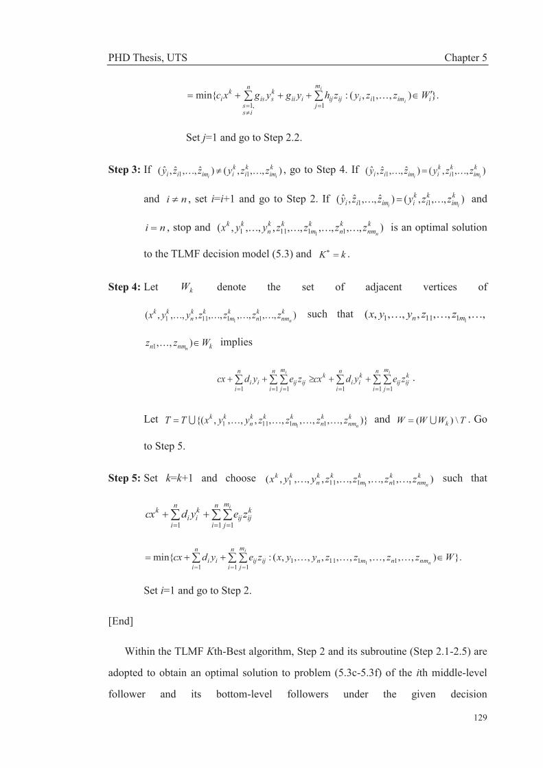
PHD Thesis, UTS Chapter 5
129
}.),,,(:min{ 11,1
iimii
m
jijijiii
n
iss
ksis
ki Wzzyzhygygxc
i
i
Set j=1 and go to Step 2.2.
Step 3: If ),,,()ˆ,,ˆ,ˆ( 11kim
ki
kiimii ii
zzyzzy , go to Step 4. If ),,,()ˆ,,ˆ,ˆ( 11kim
ki
kiimii ii
zzyzzy
and ni , set i=i+1 and go to Step 2. If ),,,()ˆ,,ˆ,ˆ( 11kim
ki
kiimii ii
zzyzzy and
ni , stop and ),,,,,,,,,,( 11111 1
knm
kn
km
kkn
kkn
zzzzyyx is an optimal solution
to the TLMF decision model (5.3) and kK .
Step 4: Let kW denote the set of adjacent vertices of
),,,,,,,,,,( 11111 1
knm
kn
km
kkn
kkn
zzzzyyx such that ,,,,,,,,(11111 mn zzyyx
knmn Wzzn),,1 implies
n
i
m
j
kijij
n
i
kii
kn
i
m
jijij
n
iii
ii
zeydcxzeydcx1 111 11
.
Let )},,,,,,,,,,{( 11111 1
knm
kn
km
kkn
kkn
zzzzyyxTT and TWWW k \)( . Go
to Step 5.
Step 5: Set k=k+1 and choose ),,,,,,,,,,( 11111 1
knm
kn
km
kkn
kkn
zzzzyyx such that
n
i
m
j
kijij
n
i
kii
k izeydcx
1 11
}.),,,,,,,,,,(:min{ 111111 11
1Wzzzzyyxzeydcx
n
i
nmnmn
n
i
m
jijij
n
iii
Set i=1 and go to Step 2.
[End]
Within the TLMF Kth-Best algorithm, Step 2 and its subroutine (Step 2.1-2.5) are
adopted to obtain an optimal solution to problem (5.3c-5.3f) of the ith middle-level
follower and its bottom-level followers under the given decision
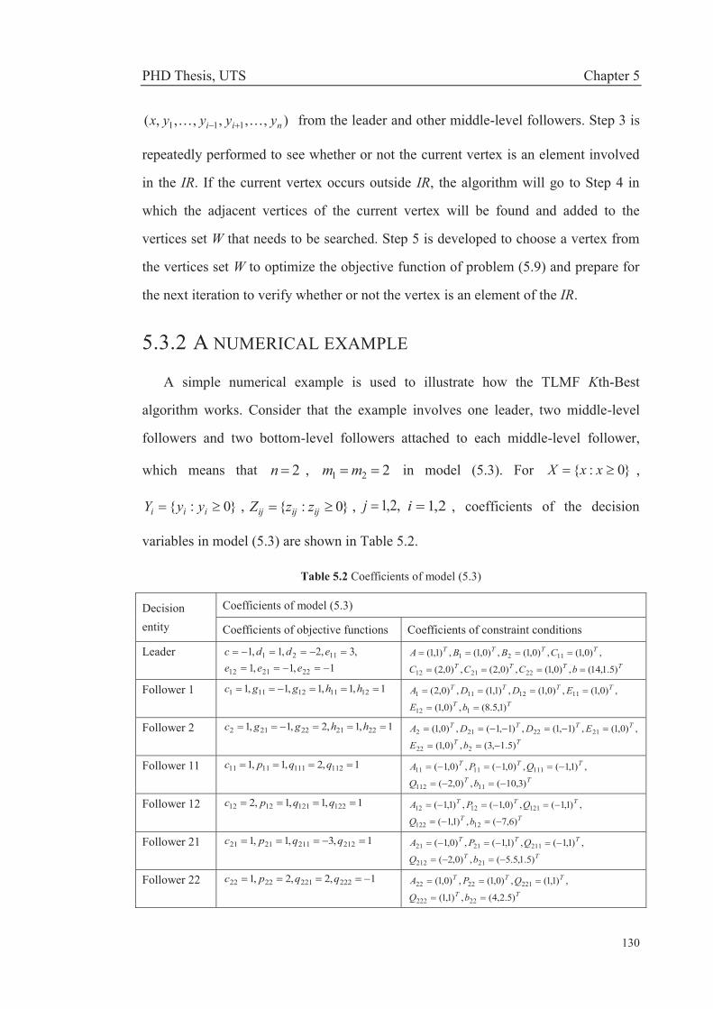
PHD Thesis, UTS Chapter 5
130
),,,,,,( 111 nii yyyyx from the leader and other middle-level followers. Step 3 is
repeatedly performed to see whether or not the current vertex is an element involved
in the IR. If the current vertex occurs outside IR, the algorithm will go to Step 4 in
which the adjacent vertices of the current vertex will be found and added to the
vertices set W that needs to be searched. Step 5 is developed to choose a vertex from
the vertices set W to optimize the objective function of problem (5.9) and prepare for
the next iteration to verify whether or not the vertex is an element of the IR.
5.3.2 A NUMERICAL EXAMPLE
A simple numerical example is used to illustrate how the TLMF Kth-Best
algorithm works. Consider that the example involves one leader, two middle-level
followers and two bottom-level followers attached to each middle-level follower,
which means that 2n , 221 mm in model (5.3). For }0:{ xxX ,
}0:{ iii yyY , }0:{ ijijij zzZ , ,2,1j 2,1i , coefficients of the decision
variables in model (5.3) are shown in Table 5.2.
Table 5.2 Coefficients of model (5.3)
Decision entity
Coefficients of model (5.3)
Coefficients of objective functions Coefficients of constraint conditions
Leader 1,1,1
,3,2,1,1
222112
1121
eeeeddc
TTTT
TTTT
bCCC
CBBA
)5.1,14(,)0,1(,)0,2(,)0,2(
,)0,1(,)0,1(,)0,1(,)1,1(
222112
1121
Follower 1 1,1,1,1,1 121112111 hhggc TT
TTTT
bE
EDDA
)1,5.8(,)0,1(
,)0,1(,)0,1(,)1,1(,)0,2(
112
1112111
Follower 2 1,1,2,1,1 222122212 hhggc TT
TTTT
bE
EDDA
)5.1,3(,)0,1(
,)0,1(,)1,1(,)1,1(,)0,1(
222
2122212
Follower 11 1,2,1,1 1121111111 qqpc TT
TTT
bQ
QPA
)3,10(,)0,2(
,)1,1(,)0,1(,)0,1(
11112
1111111
Follower 12 1,1,1,2 1221211212 qqpc TT
TTT
bQ
QPA
)6,7(,)1,1(
,)1,1(,)0,1(,)1,1(
12122
1211212
Follower 21 1,3,1,1 2122112121 qqpc TT
TTT
bQ
QPA
)5.1,5.5(,)0,2(
,)1,1(,)1,1(,)0,1(
21212
2112121
Follower 22 1,2,2,1 2222212222 qqpc TT
TTT
bQ
QPA
)5.2,4(,)1,1(
,)1,1(,)0,1(,)0,1(
22222
2212222

PHD Thesis, UTS Chapter 5
131
Detailed procedures of the TLMF Kth-Best algorithm that are executed to solve
the numerical example are shown as follows.
Iteration 1
Step 1: Set k=1 and adopt the simplex method to obtain an optimal solution to the
following linear programming problem (5.13) in the format (5.9):
}.),,,,,,(:min{ 2221121121
2
1
2
1
2
1Szzzzyyxzeydcx
i jijij
iii (5.13)
The optimal solution to problem (5.13) is ),,,,,,( 122
121
112
111
12
11
1 zzzzyyx
)2,0,5.4,5.0,5.0,1,1( and now T , W={(1,1,0.5,0.5,4.5,0,2)}. Set i=1 and go to
Step 2.
Step 2: Put 11xx , 5.0122 yy and solve the problem (5.14) of the
middle-level follower i(=1) and its bottom-level followers in the format (5.10):
)}.,(),,(:min{ 2112111
2
111
2
111 yxPzzyzhygxc
jjj
sss (5.14)
An optimal solution (1,2,3)=)ˆ,ˆ,ˆ( 12111 zzy can be obtained by Steps 2.1-2.5 of the
TLMF Kth-Best algorithm and go to Step 3.
Step 3: ),,()ˆ,ˆ,ˆ( 112
111
1112111 zzyzzy and go to Step 4.
Step 4: Find the set 1W of adjacent vertices of ),,,,,,( 122
121
112
111
12
11
1 zzzzyyx and
now ,5.0,1,0(),2,0,5.3,5.2,5.1,1,0(),2,0,3,2,5.0,1,1(),5.1,1,3,2,5.0,1,1(),5.2,0,4,1,5.0,1,1{(1W
)}5.2,0,4,2 , )}2,0,5.4,5.0,5.0,1,1{()}2,0,5.4,5.0,5.0,1,1{(TT , 11 \ WTWWW .
Go to Step 5.
Step 5: Set k=k+1=2 and choose )5.2,0,4,1,5.0,1,1(),,,,,,( 222
221
212
211
22
21
2 zzzzyyx
from the vertices set W such that

PHD Thesis, UTS Chapter 5
132
},),,,,,,(:min{
),,,,,,(
2221121121
2
1
2
1
2
1
222
221
212
211
22
21
2)1(
Wzzzzyyxzeydcx
zzzzyyxf
i jijij
iii
set i=1 and go to Step 2, and the second iteration will begin.
Iteration 2
Step 2: Put 12xx , 5.0222 yy and solve the problem (5.14). An
optimal solution (1,2,3)=)ˆ,ˆ,ˆ( 12111 zzy can be obtained by Steps 2.1-2.5 of the TLMF
Kth-Best algorithm and go to Step 3.
Step 3: ),,()ˆ,ˆ,ˆ( 212
211
2112111 zzyzzy and go to Step 4.
Step 4: Find the set 2W of adjacent vertices of ),,,,,,( 222
221
212
211
22
21
2 zzzzyyx and
now )}5.2,0,3,3,5.1,1,0(),5.2,0,3,2,5.0,1,1{(2W , )}5.2,0,4,1,5.0,1,1{(TT
)}5.2,0,4,1,5.0,1,1(),2,0,5.4,5.0,5.0,1,1{( , ),2,0,3,2,5.0,1,1(),5.1,1,3,2,5.0,1,1{(\2 TWWW
)}5.2,0,3,3,5.1,1,0(),5.2,0,3,2,5.0,1,1(),5.2,0,4,2,5.0,1,0(),2,0,5.3,5.2,5.1,1,0( . Go to Step 5.
Step 5: Set k=k+1=3 and choose )5.1,1,3,2,5.0,1,1(),,,,,,( 322
321
312
311
32
31
3 zzzzyyx from
the vertices set W such that
),,,,,,( 322
321
312
311
32
31
3)1( zzzzyyxf
},),,,,,,(:min{ 2221121121
2
1
2
1
2
1Wzzzzyyxzeydcx
i jijij
iii
set i=1 and go to Step 2, and the third iteration will begin.
Iteration 3
Step 2: Put 13xx , 5.0322 yy and solve the problem (5.14). An optimal
solution (1,2,3)=)ˆ,ˆ,ˆ( 12111 zzy is obtained by Steps 2.1-2.5 of the TLMF Kth-Best
algorithm and go to Step 3.

PHD Thesis, UTS Chapter 5
133
Step 3: Clearly, (1,2,3) =),,()ˆ,ˆ,ˆ( 312
311
3112111 zzyzzy , and ni , set i=i+1=2 and go
to Step 2.
Step 2: Put 13xx , 1311 yy and solve the problem (5.15) of the
middle-level follower i(=2) and its bottom-level followers in the format (5.10):
)}.,(),,(:min{ 1222211
2
122
2
122 yxPzzyzhygxc
jjj
sss (5.15)
An optimal solution )(0.5,1,1.5=)ˆ,ˆ,ˆ( 22212 zzy is obtained by Steps 2.1-2.5 of the
TLMF Kth-Best algorithm and go to Step 3.
Step 3: )5.1,1,5.0(),,()ˆ,ˆ,ˆ( 322
321
3222212 zzyzzy and i=n=2, stop and
)5.1,1,3,2,5.0,1,1(),,,,,,( 322
321
312
311
32
31
3 zzzzyyx is an optimal solution to the Example 5.1
and the iteration number 3kK .
An optimal solution is finally obtained to the numerical example through three
iterations, which means that three vertices are enumerated to get an optimal solution.
The objective function values of all decision entities are 5.5)1(f , 5.5)2(1f ,
5.3)2(2f , 0.9)3(
11f , 0.8)3(12f , 0)3(
21f , 5.2)3(22f . Thus, the TLMF Kth-Best
algorithm provides a convenient way to solve linear TLMF decision problems.
5.4 SOLUTION EVALUATION The proposed TLMF Kth-Best algorithm is able to find an optimal solution to the
TLMF decision model (5.3). However, it is difficult to illustrate the operations of the
complex TLMF decision-making process by the optimal solution defined by
Definition 5.9 because the solution only represents the decision result rather than the
decision-making process. In this section, a fuzzy programming approach is used to
evaluate the solution obtained and illustrate why decision entities have to achieve and
accept the final result during the TLMF decision-making process.
PHD Thesis, UTS Chapter 5
134
Within a TLMF decision-making process, each decision entity seeks to optimize
its own objective but its decision is affected by actions of others, thus, decision
entities achieve a compromised result with a possible relaxation rather than their
individual best solutions as desired. Since it is imprecise or ambiguous for decision
entities to identify a compromised result whether or not they desire it, the objective
functions can be transformed into fuzzy goals using an imprecise aspiration level.
minf and maxf are used to denote the individual best and worst results respectively
that a decision entity may achieve. Finally, the compromised objective value of the
decision entity must be involved in the interval ],[ maxmin ff . Therefore, membership
functions )( f can be elicited to characterize fuzzy goals over the domain
],[ maxmin ff for the objective functions, which can also be adopted to describe the
satisfactory degree of decision entities towards a solution or an objective value. For
example, a decision entity specifies the objective value 0f such that the satisfactory
degree is 0, that is 0)( 0f , while the value 1f of the objective function such
that 1)( 1f means that the satisfactory degree is 1. Clearly, if an objective value
f is undesired (larger) than 0f , it is defined that 0)( f ; whereas 1)( f if
an objective value f is desired (smaller) than 1f . In this study, for the sake of
simplicity, 0f and 1f are specified as max0 ff and min1 ff , and that the
membership functions are linear versions shown as Figure 5.2 although they do not
always need to be linear. Also, note that in this research the satisfactory degree
1)( f if there exists maxmin ff .

PHD Thesis, UTS Chapter 5
135
0
μ(f)
1.0
1f 0f Figure 5.2 Linear membership function
(1) The membership function of the leader
The individual best objective value of the leader is:
:),,,,,,,,,,(min{ 11111)1(min1
1 nnmnmn zzzzyyxfff
}.),,,,,,,,,,( 11111 1Szzzzyyx
nnmnmn
The individual worst objective value is:
:),,,,,,,,,,(max{ 11111)1(max0
1 nnmnmn zzzzyyxfff
}.),,,,,,,,,,( 11111 1Szzzzyyx
nnmnmn
The corresponding linear membership function )( )1(f is defined as:
.,
,,
,1
,0
)(1)1(
0)1(1
0)1(
01
0)1()1(
fffff
ff
fffff (5.16)
)( )1(f can be used to denote the satisfactory degree of the leader towards an
objective value )1(f . 0)( 0f implies that the satisfactory degree of the leader is
0 when the objective value 0)1( ff , while the objective value 1)1( ff such that
1)( 1f means that the satisfactory degree of the leader becomes 1.
PHD Thesis, UTS Chapter 5
136
(2) The membership function of the middle-level follower i
The middle-level follower i makes its decision under the given decisions
),,,,,,( 111 nii yyyyx from the leader and other middle-level followers, thus, its
individual best objective value is:
:),,,,,,,,,,(min{ 1111)2(min1
iiminiiiiii zzyyyyyxfff
)}.,,,,,,(),,,( 1111 niiiimii yyyyxSzzyi
The individual worst objective value is:
:),,,,,,,,,,(max{ 1111)2(max0
iiminiiiiii zzyyyyyxfff
)}.,,,,,,(),,,( 1111 niiiimii yyyyxSzzyi
The corresponding linear membership function )( )2(ii f is defined as:
.,
,,
,1
,0
)(1)2(
0)2(1
0)2(
01
0)2()2(
ii
iii
ii
ii
iiii
fffff
ff
fffff (5.17)
)( )2(ii f can be used to denote the satisfactory degree of the middle-level
follower i towards an objective value )2(if . 0)( 0
ii f implies that the satisfactory
degree of the middle-level follower i is 0 when the objective value 0)2(ii ff ,
whereas the objective value 1)2(ii ff such that 1)( 1
ii f means that the
satisfactory degree becomes 1.

PHD Thesis, UTS Chapter 5
137
(3) The membership function of the bottom-level follower ij
The bottom-level follower ij makes its decision under the given decision
),,,,,,,( )1()1(1 iimjijiii zzzzyx from the leader, the middle-level follower i and
its own counterparts, thus, its individual best objective value is:
:),,,,,,,,(min{ )1()1(1)3(min1
iimjiijjiiiijijij zzzzzyxfff
)}.,,,,,,,( )1()1(1 iimjijiiiijij zzzzyxSz
The individual worst objective value is:
:),,,,,,,,(max{ )1()1(1)3(max0
iimjiijjiiiijijij zzzzzyxfff
)}.,,,,,,,( )1()1(1 iimjijiiiijij zzzzyxSz
The corresponding linear membership function )( )3(ijij f is defined as:
.,
,,
,1
,0
)(1)3(
0)3(1
0)3(
01
0)3()3(
ijij
ijijij
ijij
ijij
ijijijij
fffff
ff
ffff
f (5.18)
)( )3(ijij f can be used to denote the satisfactory degree of the bottom-level
follower ij towards an objective value )3(ijf . 0)( 0
ijij f implies that the satisfactory
degree is 0 when the objective value 0)3(ijij ff , while the objective value 1)3(
ijij ff
such that 1)( 1ijij f means that the satisfactory degree is 1.
The proposed evaluation method based on fuzzy programming is applied to assess
the solution to the numerical example in Section 5.3.2. For the leader,
3)2,0,5.4,5.0,5.0,1,1()1(min1 fff and 5.9)5.2,0,3,3,5.0,1,0()1(max0 fff ,
thus, by the formula (5.16) the leader’s satisfactory degrees are 1.0, 0.92 and 0.62
respectively towards the vertices )2,0,5.4,5.0,5.0,1,1(),,,,,,( 122
121
112
111
12
11
1 zzzzyyx ,
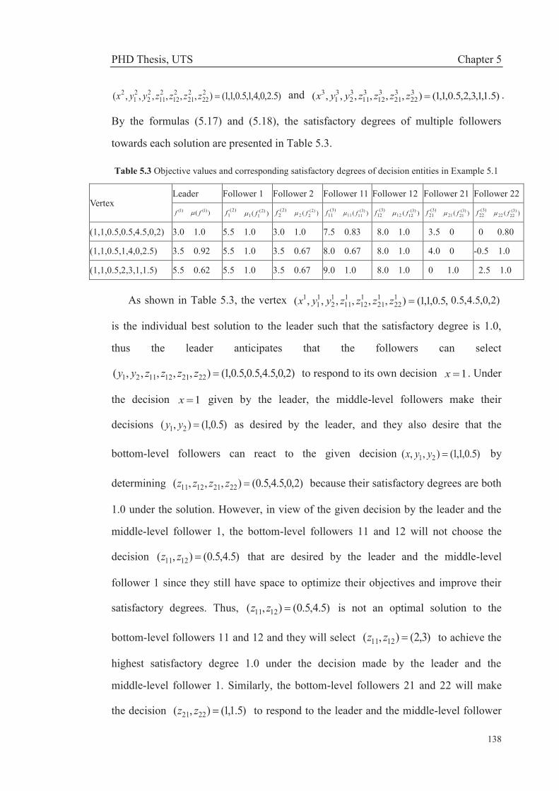
PHD Thesis, UTS Chapter 5
138
)5.2,0,4,1,5.0,1,1(),,,,,,( 222
221
212
211
22
21
2 zzzzyyx and )5.1,1,3,2,5.0,1,1(),,,,,,( 322
321
312
311
32
31
3 zzzzyyx .
By the formulas (5.17) and (5.18), the satisfactory degrees of multiple followers
towards each solution are presented in Table 5.3.
Table 5.3 Objective values and corresponding satisfactory degrees of decision entities in Example 5.1
Vertex Leader Follower 1 Follower 2 Follower 11 Follower 12 Follower 21 Follower 22
)1(f )( )1(f )2(1f )( )2(
11 f )2(2f )( )2(
22 f )3(11f )( )3(
1111 f )3(12f )( )3(
1212 f )3(21f )( )3(
2121 f )3(22f )( )3(
2222 f
(1,1,0.5,0.5,4.5,0,2) 3.0 1.0 5.5 1.0 3.0 1.0 7.5 0.83 8.0 1.0 3.5 0 0 0.80
(1,1,0.5,1,4,0,2.5) 3.5 0.92 5.5 1.0 3.5 0.67 8.0 0.67 8.0 1.0 4.0 0 -0.5 1.0
(1,1,0.5,2,3,1,1.5) 5.5 0.62 5.5 1.0 3.5 0.67 9.0 1.0 8.0 1.0 0 1.0 2.5 1.0
As shown in Table 5.3, the vertex ,5.0,1,1(),,,,,,( 122
121
112
111
12
11
1 zzzzyyx )2,0,5.4,5.0
is the individual best solution to the leader such that the satisfactory degree is 1.0,
thus the leader anticipates that the followers can select
)2,0,5.4,5.0,5.0,1(),,,,,( 2221121121 zzzzyy to respond to its own decision 1x . Under
the decision 1x given by the leader, the middle-level followers make their
decisions )5.0,1(),( 21 yy as desired by the leader, and they also desire that the
bottom-level followers can react to the given decision )5.0,1,1(),,( 21 yyx by
determining )2,0,5.4,5.0(),,,( 22211211 zzzz because their satisfactory degrees are both
1.0 under the solution. However, in view of the given decision by the leader and the
middle-level follower 1, the bottom-level followers 11 and 12 will not choose the
decision )5.4,5.0(),( 1211 zz that are desired by the leader and the middle-level
follower 1 since they still have space to optimize their objectives and improve their
satisfactory degrees. Thus, )5.4,5.0(),( 1211 zz is not an optimal solution to the
bottom-level followers 11 and 12 and they will select )3,2(),( 1211 zz to achieve the
highest satisfactory degree 1.0 under the decision made by the leader and the
middle-level follower 1. Similarly, the bottom-level followers 21 and 22 will make
the decision )5.1,1(),( 2221 zz to respond to the leader and the middle-level follower

PHD Thesis, UTS Chapter 5
139
2. The leader and the middle-level followers have to reduce their individual
satisfactory degrees to bend to the increase in the satisfactory degrees of the
bottom-level followers throughout the TLMF decision-making process. In this way,
the decision entities finally achieve an optimal solution
)5.1,1,3,2,5.0,1,1(),,,,,,( 322
321
312
311
32
31
3 zzzzyyx , under which the satisfactory degrees of all
the bottom-level followers go up to 1.0.
Although the satisfactory degrees of the leader and the middle-level follower 2
drop to 0.62 and 0.67 respectively, the numbers become the highest satisfactory
degrees for them under the reference-based relationship between all decision entities.
In real-world cases, the situation indicates that higher satisfactory degrees of the
leader and the middle-level follower 2 cannot be achieved under the current decision
conditions unless they may persuade the bottom-level followers to cooperate with
them and to reduce the corresponding satisfactory degrees. For example, if the
bottom-level followers 11, 21 and 22 are willing to accept their respective satisfactory
degrees 0.83, 0 and 0.80, the solution to the numerical example in Section 5.3.2
would be )2,0,5.4,5.0,5.0,1,1(),,,,,,( 122
121
112
111
12
11
1 zzzzyyx , which ensures that the
corresponding satisfactory degrees of the leader and the bottom-level follower 2 rise
up to 1.0. Otherwise, they have to adjust the current decision context through
changing objective functions or constraint conditions to generate a new round of the
decision-making process. The evaluation criterion will be applied to deal with a
production-inventory planning problem in the following Section 5.5.
5.5 CASE STUDY In this section, a case study on production-inventory planning is handled using the
proposed TLMF decision-making techniques.
PHD Thesis, UTS Chapter 5
140
5.5.1 CASE DESCRIPTION
Nowadays, manufacturers usually work in a distributed or decentralized manner in
a complex supply chain network comprising of suppliers, sales and logistics
companies, customers and other specialized service functions (Chan & Chan 2010).
Researchers as well as practitioners in manufacturing industries have placed
importance on developing production and inventory control capabilities to enhance
their market position in supply chain management (Sana 2011), which demands that
manufacturing enterprises have to make right decisions on scheduling of their
production and allocation of inventory to satisfy market requirements, shorten
delivery time and reduce total production costs (Askin, Baffo & Xia 2014; Chang, Li
& Chiang 2014; Tan, Lee & Goh 2012). Therefore, it is increasingly important to
have efficient and easily-applicable models and solution methods to describe and
solve related production-inventory decision problems (Berling & Marklund 2014; Ho
& Hsiao 2014) although modeling deception in a real-world conflict situation is
usually difficult (Li & Cruz Jr 2009).
In this section, the proposed TLMF decision techniques are applied to handle a
production-inventory planning problem within a real-world conglomerate enterprise.
The conglomerate is composed of a sales company, two logistics centers and two
manufacturing factories attached to each logistics center, which are distributed
throughout a three-stage hierarchical supply chain. The three-level hierarchical
structure of the conglomerate is shown in Figure 5.3. Specifically, the sales company
covers products marketing of the enterprise and has an independent products
warehouse to satisfy market demand and shorten time-to-market. Both logistics
centers also hold a certain amount of products inventory to respond to market
requirements and reduce the inventory pressure of the sales company. According to
market requirements and the holding inventories of the sales company and the
logistics centers, the manufacturing factories are responsible for the production
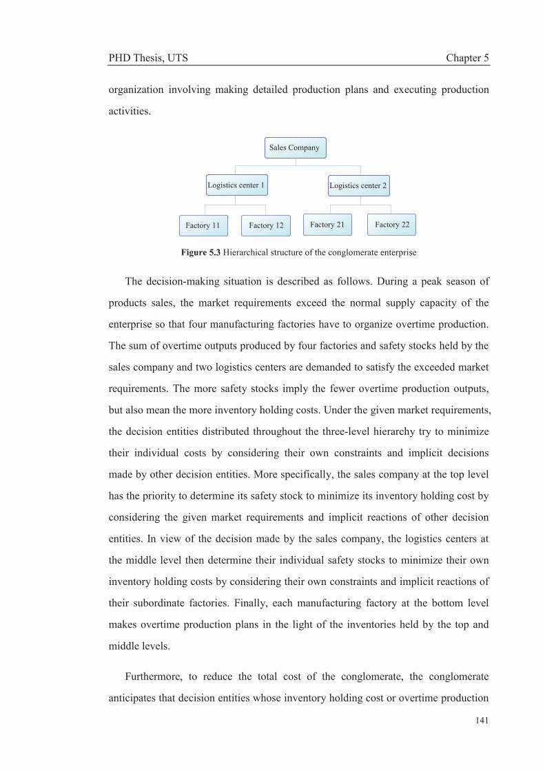
PHD Thesis, UTS Chapter 5
141
organization involving making detailed production plans and executing production
activities.
Sales Company
Logistics center 1 Logistics center 2
Factory 11 Factory 12 Factory 21 Factory 22
Figure 5.3 Hierarchical structure of the conglomerate enterprise
The decision-making situation is described as follows. During a peak season of
products sales, the market requirements exceed the normal supply capacity of the
enterprise so that four manufacturing factories have to organize overtime production.
The sum of overtime outputs produced by four factories and safety stocks held by the
sales company and two logistics centers are demanded to satisfy the exceeded market
requirements. The more safety stocks imply the fewer overtime production outputs,
but also mean the more inventory holding costs. Under the given market requirements,
the decision entities distributed throughout the three-level hierarchy try to minimize
their individual costs by considering their own constraints and implicit decisions
made by other decision entities. More specifically, the sales company at the top level
has the priority to determine its safety stock to minimize its inventory holding cost by
considering the given market requirements and implicit reactions of other decision
entities. In view of the decision made by the sales company, the logistics centers at
the middle level then determine their individual safety stocks to minimize their own
inventory holding costs by considering their own constraints and implicit reactions of
their subordinate factories. Finally, each manufacturing factory at the bottom level
makes overtime production plans in the light of the inventories held by the top and
middle levels.
Furthermore, to reduce the total cost of the conglomerate, the conglomerate
anticipates that decision entities whose inventory holding cost or overtime production
PHD Thesis, UTS Chapter 5
142
cost is lower are able to keep more inventories or manufacture more production
outputs. Thus, the conglomerate makes some management strategies to intervene and
reconcile the decision process of its subordinate decision entities. For example, the
conglomerate claims that each logistics center should take the inventory determined
by the other logistics center as a reference when making its own decisions. If the
inventory of a logistics center is less than the other, it means the less inventory
holding cost but implies that the logistics center is demanded to undertake an
opportunity cost for its own decision on holding less inventory. Also, each factory
needs to reference the production plans made by other counterparts attached to the
same logistics center when making its own production plans. If the production outputs
of a factory are less than the other, it means the less overtime production costs but
implies that the factory needs to cover an opportunity cost for its own decision on less
production outputs. In addition, the sales company is demanded to afford the
marketing cost and backlogging cost of the conglomerate. However, to reduce the
total cost to the sales company, the conglomerate demands that both logistics centers
must share part of the inventory holding cost and compensate for the marketing cost
of the sales company. Similarly, to reduce the pressure of overtime production, the
factories at the bottom level are also demanded to compensate the inventory holding
cost of their superior logistics center to encourage it to keep more safety stocks.
Therefore, under the current decision situation, the decision entities will try to
minimize their individual overall costs by making their individual decisions, and the
decision processes are executed sequentially, interactively and repeatedly within the
tri-level hierarchy until the equilibrium is achieved among them.
This case clearly describes a TLMF decision process which includes one leader
(the sales company), two middle-level followers (the logistics centers) and two
bottom-level followers (the manufacturing factories) attached to each middle-level
follower. The leader, the middle-level followers and the bottom-level followers make
their individual decisions in sequence, and each decision entity cannot control
decisions of the others but is affected by their reactions. It is noticeable that the
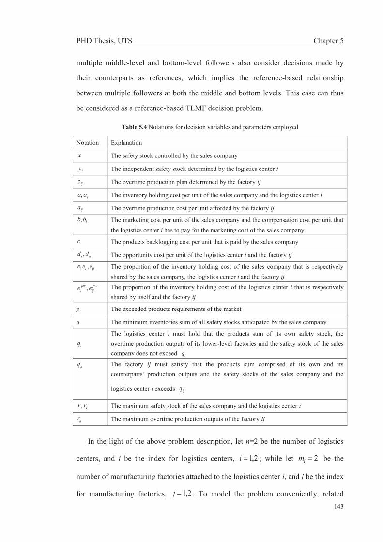
PHD Thesis, UTS Chapter 5
143
multiple middle-level and bottom-level followers also consider decisions made by
their counterparts as references, which implies the reference-based relationship
between multiple followers at both the middle and bottom levels. This case can thus
be considered as a reference-based TLMF decision problem.
Table 5.4 Notations for decision variables and parameters employed
Notation Explanation
x The safety stock controlled by the sales company
iy The independent safety stock determined by the logistics center i
ijz The overtime production plan determined by the factory ij
iaa, The inventory holding cost per unit of the sales company and the logistics center i
ija The overtime production cost per unit afforded by the factory ij
ibb, The marketing cost per unit of the sales company and the compensation cost per unit that the logistics center i has to pay for the marketing cost of the sales company
c The products backlogging cost per unit that is paid by the sales company
iji dd , The opportunity cost per unit of the logistics center i and the factory ij
iji eee ,, The proportion of the inventory holding cost of the sales company that is respectively
shared by the sales company, the logistics center i and the factory ij pw
ijpw
i ee , The proportion of the inventory holding cost of the logistics center i that is respectively shared by itself and the factory ij
p The exceeded products requirements of the market
q The minimum inventories sum of all safety stocks anticipated by the sales company
iq
The logistics center i must hold that the products sum of its own safety stock, the overtime production outputs of its lower-level factories and the safety stock of the sales company does not exceed iq
ijq The factory ij must satisfy that the products sum comprised of its own and its
counterparts’ production outputs and the safety stocks of the sales company and the
logistics center i exceeds ijq
irr, The maximum safety stock of the sales company and the logistics center i
ijr The maximum overtime production outputs of the factory ij
In the light of the above problem description, let n=2 be the number of logistics
centers, and i be the index for logistics centers, 2,1i ; while let 2im be the
number of manufacturing factories attached to the logistics center i, and j be the index
for manufacturing factories, 2,1j . To model the problem conveniently, related
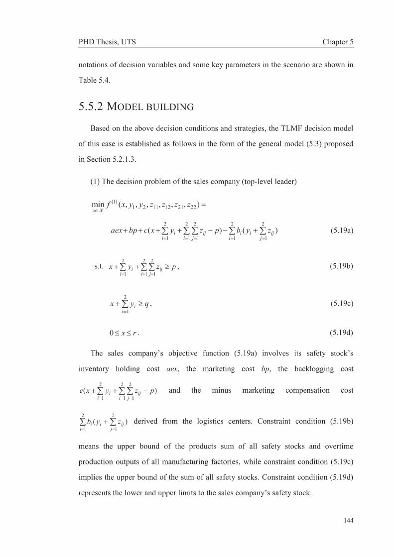
PHD Thesis, UTS Chapter 5
144
notations of decision variables and some key parameters in the scenario are shown in
Table 5.4.
5.5.2 MODEL BUILDING
Based on the above decision conditions and strategies, the TLMF decision model
of this case is established as follows in the form of the general model (5.3) proposed
in Section 5.2.1.3.
(1) The decision problem of the sales company (top-level leader)
),,,,,,(min 2221121121)1( zzzzyyxf
Xx
2
1
2
1
2
1
2
1
2
1)()(
i jijii
i jij
ii zybpzyxcbpaex (5.19a)
s.t. pzyxi j
iji
i
2
1
2
1
2
1, (5.19b)
qyxi
i
2
1, (5.19c)
rx0 . (5.19d)
The sales company’s objective function (5.19a) involves its safety stock’s
inventory holding cost aex, the marketing cost bp, the backlogging cost
)(2
1
2
1
2
1pzyxc
i jij
ii and the minus marketing compensation cost
2
1
2
1)(
i jijii zyb derived from the logistics centers. Constraint condition (5.19b)
means the upper bound of the products sum of all safety stocks and overtime
production outputs of all manufacturing factories, while constraint condition (5.19c)
implies the upper bound of the sum of all safety stocks. Constraint condition (5.19d)
represents the lower and upper limits to the sales company’s safety stock.

PHD Thesis, UTS Chapter 5
145
(2) The decision problem of the logistics center (middle-level follower) i
)(),,,,(min2
12121
)2(
jijiiiiii
pwiiiiiYy
zybxaeydyeazzyyxfii
(5.19e)
s.t. ij
iji
i qzyx2
1
2
1, (5.19f)
ii ry0 . (5.19g)
The objective function (5.19e) of the logistics center i involves its safety stock
holding cost ipwii yea , the opportunity cost ii yd , the shared inventory holding cost
xaei of the sales company’s safety stock and the marketing compensation cost
)(2
1jijii zyb paid to the sales company. Note that 121 yyy and 212 yyy .
Constraint condition (5.19f) reflects the upper bound of the products sum consisting
of all safety stocks and the overtime production outputs of the manufacturing factories
attached to the middle-level follower i. Constraint condition (5.19g) represents the
lower and upper limits to the safety stock of the logistics center i.
(3) The decision problem of the manufacturing factory (bottom-level follower) ij
ipwijiijijijijijiiiijZz
yeaxaezdzazzyxfijij
),,,(min 21)3( (5.19h)
s.t. ijj
iji qzyx2
1, (5.19i)
ijij rz0 . (5.19j)
The objective function (5.19h) of the manufacturing factory ij involves its
overtime production cost ijij za , the opportunity cost ijij zd , and the shared
inventory holding cost xaeij and ipwiji yea respectively for the safety stocks of the
sales company and the logistics center i. Note that 121 iii zzz and
212 iii zzz . Constraint condition (5.19i) reflects the upper bound of the products

PHD Thesis, UTS Chapter 5
146
sum consisting of overtime production outputs of the manufacturing factories attached
to the logistics center i and safety stocks of the sales company and the logistics center
i. Constraint condition (5.19j) represents the lower and upper limits to the overtime
production outputs of the manufacturing factory ij.
This TLMF decision model (5.19) describes the real-world production and
inventory decision problem which is a concretization of the general model (5.3)
proposed in Section 5.2.1.3. The TLMF Kth-Best algorithm is then adopted to solve
the model by a numerical experiment. Also, the fuzzy programming approach is used
to evaluate the solutions obtained.
5.5.3 NUMERICAL EXPERIMENT AND RESULTS ANALYSIS
This section shows the computational results achieved by the proposed TLMF
Kth-Best algorithm and the fuzzy programming approach. The experimental data
employed for the model (5.19) is provided in Tables 5.5-5.7.
Table 5.5 Data for the sales company
a b c e p q r
5.0 2.0 2.0 0.20 9.0 3.5 2.5
Table 5.6 Data for the logistics centers
i ia ib id ie pwie iq ir
1 4.0 1.0 4.0 0.20 0.50 8.0 1.0
2 4.0 3.0 4.0 0.20 0.50 6.0 0.50
Table 5.7 Data for the manufacturing factories
i j ija ijd ije pwije ijq ijr
1 1 1.0 2.0 0.10 0.25 7.0 3.0
1 2 3.0 2.0 0.10 0.25 7.0 3.0
2 1 2.0 3.0 0.10 0.25 4.0 1.0
2 2 4.0 3.0 0.10 0.25 4.0 2.0
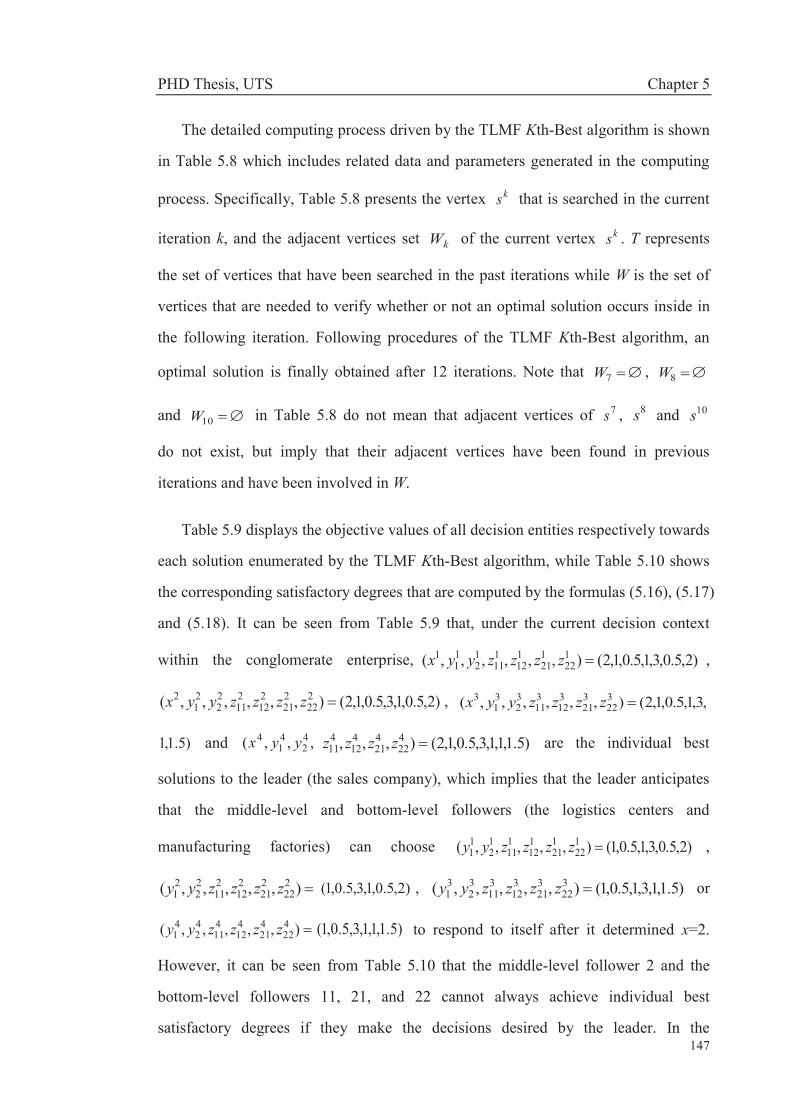
PHD Thesis, UTS Chapter 5
147
The detailed computing process driven by the TLMF Kth-Best algorithm is shown
in Table 5.8 which includes related data and parameters generated in the computing
process. Specifically, Table 5.8 presents the vertex ks that is searched in the current
iteration k, and the adjacent vertices set kW of the current vertex ks . T represents
the set of vertices that have been searched in the past iterations while W is the set of
vertices that are needed to verify whether or not an optimal solution occurs inside in
the following iteration. Following procedures of the TLMF Kth-Best algorithm, an
optimal solution is finally obtained after 12 iterations. Note that 7W , 8W
and 10W in Table 5.8 do not mean that adjacent vertices of 7s , 8s and 10s
do not exist, but imply that their adjacent vertices have been found in previous
iterations and have been involved in W.
Table 5.9 displays the objective values of all decision entities respectively towards
each solution enumerated by the TLMF Kth-Best algorithm, while Table 5.10 shows
the corresponding satisfactory degrees that are computed by the formulas (5.16), (5.17)
and (5.18). It can be seen from Table 5.9 that, under the current decision context
within the conglomerate enterprise, )2,5.0,3,1,5.0,1,2(),,,,,,( 122
121
112
111
12
11
1 zzzzyyx ,
)2,5.0,1,3,5.0,1,2(),,,,,,( 222
221
212
211
22
21
2 zzzzyyx , ,3,1,5.0,1,2(),,,,,,( 322
321
312
311
32
31
3 zzzzyyx
)5.1,1 and ,,,( 42
41
4 yyx )5.1,1,1,3,5.0,1,2(),,, 422
421
412
411 zzzz are the individual best
solutions to the leader (the sales company), which implies that the leader anticipates
that the middle-level and bottom-level followers (the logistics centers and
manufacturing factories) can choose )2,5.0,3,1,5.0,1(),,,,,( 122
121
112
111
12
11 zzzzyy ,
),,,,,( 222
221
212
211
22
21 zzzzyy )2,5.0,1,3,5.0,1( , )5.1,1,3,1,5.0,1(),,,,,( 3
22321
312
311
32
31 zzzzyy or
),,,,,( 422
421
412
411
42
41 zzzzyy )5.1,1,1,3,5.0,1( to respond to itself after it determined x=2.
However, it can be seen from Table 5.10 that the middle-level follower 2 and the
bottom-level followers 11, 21, and 22 cannot always achieve individual best
satisfactory degrees if they make the decisions desired by the leader. In the
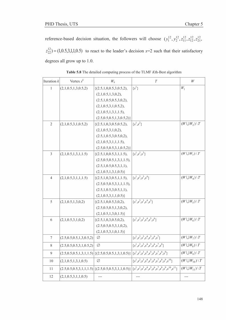
PHD Thesis, UTS Chapter 5
148
reference-based decision situation, the followers will choose ,,,,,( 1221
1212
1211
122
121 zzzyy
)5.0,1,1,3,5.0,1()1222z to react to the leader’s decision x=2 such that their satisfactory
degrees all grow up to 1.0.
Table 5.8 The detailed computing process of the TLMF Kth-Best algorithm
Iteration k Vertex sk Wk T W
1 (2,1,0.5,1,3,0.5,2) {(2.5,1,0,0.5,3,0.5,2), (2,1,0.5,1,3,0,2),
(2.5,1,0.5,0.5,3,0,2), (2,1,0.5,3,1,0.5,2), (2,1,0.5,1,3,1,1.5), (2.5,0.5,0.5,1,3,0.5,2)}
{s1} 1W
2 (2,1,0.5,3,1,0.5,2) {(2.5,1,0,3,0.5,0.5,2), (2,1,0.5,3,1,0,2), (2.5,1,0.5,3,0.5,0,2), (2,1,0.5,3,1,1,1.5), (2.5,0.5,0.5,3,1,0.5,2)}
{s1,s2} TWW \)( 2
3 (2,1,0.5,1,3,1,1.5) {(2.5,1,0,0.5,3,1,1.5), (2.5,0.5,0.5,1,3,1,1.5), (2.5,1,0.5,0.5,3,1,1), (2,1,0.5,1,3,1,0.5)}
{s1,s2,s3} TWW \)( 3
4 (2,1,0.5,3,1,1,1.5) {(2.5,1,0,3,0.5,1,1.5), (2.5,0.5,0.5,3,1,1,1.5), (2.5,1,0.5,3,0.5,1,1), (2,1,0.5,3,1,1,0.5)}
{s1,s2,s3,s4} TWW \)( 4
5 (2,1,0.5,1,3,0,2) {(2.5,1,0,0.5,3,0,2), (2.5,0.5,0.5,1,3,0,2), (2,1,0.5,1,3,0,1.5)}
{s1,s2,s3,s4,s5} TWW \)( 5
6 (2,1,0.5,3,1,0,2) {(2.5,1,0,3,0.5,0,2), (2.5,0.5,0.5,3,1,0,2), (2,1,0.5,3,1,0,1.5)}
{s1,s2,s3,s4,s5,s6} TWW \)( 6
7 (2.5,0.5,0.5,1,3,0.5,2) {s1,s2,s3,s4,s5,s6,s7} TWW \)( 7
8 (2.5,0.5,0.5,3,1,0.5,2) {s1,s2,s3,s4,s5,s6,s7,s8} TWW \)( 8
9 (2.5,0.5,0.5,1,3,1,1.5) {(2.5,0.5,0.5,1,3,1,0.5)} {s1,s2,s3,s4,s5,s6,s7,s8,s9} TWW \)( 9
10 (2,1,0.5,1,3,1,0.5) {s1,s2,s3,s4,s5,s6,s7,s8,s9,s10} TWW \)( 10
11 (2.5,0.5,0.5,3,1,1,1.5) {(2.5,0.5,0.5,3,1,1,0.5)} {s1,s2,s3,s4,s5,s6,s7,s8,s9,s10,s11} TWW \)( 11
12 (2,1,0.5,3,1,1,0.5) --- --- ---

PHD Thesis, UTS Chapter 5
149
Table 5.9 Solutions and objective values of decision entities
Iteration k Vertex sk )1(f )2(1f )2(
2f )3(11f )3(
12f )3(21f )3(
22f
1 (2,1,0.5,1,3,0.5,2) 8.0 7.0 14.0 7.0 7.0 7.0 5.0
2 (2,1,0.5,3,1,0.5,2) 8.0 7.0 14.0 1.0 9.0 7.0 5.0
3 (2,1,0.5,1,3,1,1.5) 8.0 7.0 14.0 7.0 7.0 5.0 6.0
4 (2,1,0.5,3,1,1,1.5) 8.0 7.0 14.0 1.0 9.0 5.0 6.0
5 (2,1,0.5,1,3,0,2) 8.5 7.0 12.5 7.0 7.0 7.5 3.5
6 (2,1,0.5,3,1,0,2) 8.5 7.0 12.5 1.0 9.0 7.5 3.5
7 (2.5,0.5,0.5,1,3,0.5,2) 9.0 8.0 12.5 6.75 6.75 7.25 5.25
8 (2.5,0.5,0.5,3,1,0.5,2) 9.0 8.0 12.5 0.75 8.75 7.25 5.25
9 (2.5,0.5,0.5,1,3,1,1.5) 9.0 8.0 12.5 6.75 6.75 5.25 6.25
10 (2,1,0.5,1,3,1,0.5) 9.0 7.0 11.0 7.0 7.0 2.0 5.0
11 (2.5,0.5,0.5,3,1,1,1.5) 9.0 8.0 12.5 0.75 8.75 5.25 6.25
12 (2,1,0.5,3,1,1,0.5) 9.0 7.0 11.0 1.0 9.0 2.0 5.0
More specifically, for the given decision )1,2(),( 1yx by the leader and the
middle-level follower 1, the bottom-level followers 11 and 12 achieve a Nash
equilibrium solution )1,3(),( 1211 zz to respond to the leader and the middle-level
follower 1. Similarly, for the given decision )5.0,2(),( 2yx by the leader and the
middle-level follower 2, the bottom-level followers 21 and 22 achieve a Nash
equilibrium solution )5.0,1(),( 2221 zz to respond to the leader and the
middle-level follower 2. Therefore, )1,3,1(),,( 12111 zzy and ),,( 22212 zzy
)5.0,1,5.0( are the optimal solutions respectively for the middle-level follower i
(i=1,2) and its bottom-level followers under the given decision 2x by the leader.
Also, for the given decision x=2 by the leader, )5.0,1(),( 21 yy is the optimal
solution for the middle-level followers while taking into account implicit reactions of
their respective bottom-level followers. Therefore, ),,,,,,( 1222
1221
1212
1211
122
121
12 zzzzyyx
)5.0,1,1,3,5.0,1,2( is an optimal solution to the production-inventory planning problem.

PHD Thesis, UTS Chapter 5
150
Table 5.10 The satisfactory degree of decision entities towards solutions
Iteration
k
Leader Follower 1 Follower 2 Follower 11 Follower 12 Follower 21 Follower 22
1f 0f )( )1(f 11f 0
1f )( )2(11 f 1
2f 02f )( )2(
22 f 111f 0
11f )( )3(1111 f 1
12f 012f )( )3(
1212 f 121f 0
21f )( )3(2121 f 1
22f 022f )( )3(
2222 f
1 8.0 11.5 1.0 7.0 9.5 1.0 11.0 15.0 0.25 5.0 7.0 0 7.0 7.0 1.0 6.5 7.5 0.5 4.0 5.0 0
2 8.0 11.5 1.0 7.0 9.5 1.0 11.0 15.0 0.25 1.0 1.0 1.0 9.0 11.0 1.0 6.5 7.5 0.5 4.0 5.0 0
3 8.0 11.5 1.0 7.0 9.5 1.0 11.0 15.0 0.25 5.0 7.0 0 7.0 7.0 1.0 5.0 6.0 1.0 5.0 6.5 0.33
4 8.0 11.5 1.0 7.0 9.5 1.0 11.0 15.0 0.25 1.0 1.0 1.0 9.0 11.0 1.0 5.0 6.0 1.0 5.0 6.5 0.33
5 8.0 11.5 0.86 7.0 9.5 1.0 11.0 15.0 0.63 5.0 7.0 0 7.0 7.0 1.0 6.5 7.5 0 3.0 3.5 0
6 8.0 11.5 0.86 7.0 9.5 1.0 11.0 15.0 0.63 1.0 1.0 1.0 9.0 11.0 1.0 6.5 7.5 0 3.0 3.5 0
7 8.0 11.5 0.71 7.0 9.5 0.6 8.0 13.5 0.18 4.75 6.75 0 6.75 6.75 1.0 6.75 7.75 0.5 3.75 5.25 0
8 8.0 11.5 0.71 7.0 9.5 0.6 8.0 13.5 0.18 0.75 0.75 1.0 8.75 10.75 1.0 6.75 7.75 0.5 3.75 5.25 0
9 8.0 11.5 0.71 7.0 9.5 0.6 8.0 13.5 0.18 4.75 6.75 0 6.75 6.75 1.0 5.25 6.25 1.0 4.75 6.75 0.25
10 8.0 11.5 0.71 7.0 9.5 1.0 11.0 15.0 1.0 5.0 7.0 0 7.0 7.0 1.0 2.0 2.0 1.0 5.0 6.5 1.0
11 8.0 11.5 0.71 7.0 9.5 0.6 8.0 13.5 0.18 0.75 0.75 1.0 8.75 10.75 1.0 5.25 6.25 1.0 4.75 6.75 0.25
12 8.0 11.5 0.71 7.0 9.5 1.0 11.0 15.0 1.0 1.0 1.0 1.0 9.0 11.0 1.0 2.0 2.0 1.0 5.0 6.5 1.0

PHD Thesis, UTS Chapter 5
151
Although the leader’s satisfactory degree has dropped to 0.71 under the solution
)5.0,1,1,3,5.0,1,2(),,,,,,( 1222
1221
1212
1211
122
121
12 zzzzyyx , the leader cannot obtain a better
objective value or a higher satisfactory degree by moving away from the vertex over
the IR. Therefore, within the real-world case study, the solution
)5.0,1,1,3,5.0,1,2(),,,,,,( 1222
1221
1212
1211
122
121
12 zzzzyyx is the optimal solution to the TLMF
decision model (5.19), which means a final compromised result among all decision
entities under the current decision context in the conglomerate enterprise. This TLMF
hierarchical decision situation indicates that the leader may not achieve an individual
optimal solution under the constraint region even though it has priority in making
decisions, since its decisions are determined by implicit reactions of the followers.
Moreover, the decision process and results of an TLMF decision problem are affected
by the reference-based relationship between multiple followers at the same level. In
summary, the proposed TLMF decision techniques provide an effective way to model
and solve real-world TLMF decision problems and to recognize the satisfactory
degree of decision entities towards solutions.
Furthermore, by the optimal solution, it can be analyzed that whether or not the
conglomerate employed practical and effective management strategies to balance the
production-inventory planning among its subordinate sales company, logistics centers
and manufacturing factories. Based on the given experimental data in Tables 5.5-5.7,
the contrastive analysis between the upper limits to the holding inventory or overtime
production capacity of each decision entity and the final solution is shown as Figure
5.4. It can be seen from Figure 5.4 that the holding inventories of the logistics centers
peak at their respective upper limits. Also, the production outputs of the
manufacturing factories 11 and 21 reach their maximum overtime production
capacities respectively. In contrast, the holding inventory or overtime production
outputs of other decision entities are less or much less than their corresponding upper
limits. These results indicate that decision entities whose inventory holding cost or
overtime production cost is lower prefer to keep more inventories or manufacture
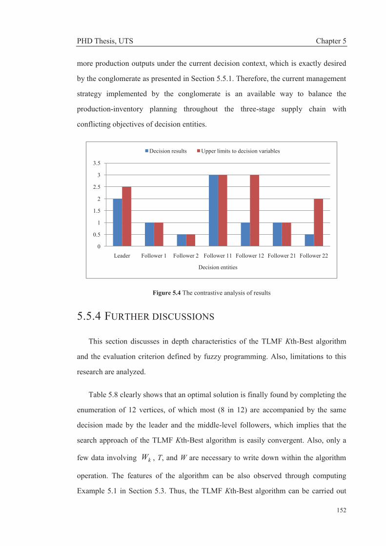
PHD Thesis, UTS Chapter 5
152
more production outputs under the current decision context, which is exactly desired
by the conglomerate as presented in Section 5.5.1. Therefore, the current management
strategy implemented by the conglomerate is an available way to balance the
production-inventory planning throughout the three-stage supply chain with
conflicting objectives of decision entities.
Figure 5.4 The contrastive analysis of results
5.5.4 FURTHER DISCUSSIONS
This section discusses in depth characteristics of the TLMF Kth-Best algorithm
and the evaluation criterion defined by fuzzy programming. Also, limitations to this
research are analyzed.
Table 5.8 clearly shows that an optimal solution is finally found by completing the
enumeration of 12 vertices, of which most (8 in 12) are accompanied by the same
decision made by the leader and the middle-level followers, which implies that the
search approach of the TLMF Kth-Best algorithm is easily convergent. Also, only a
few data involving kW , T, and W are necessary to write down within the algorithm
operation. The features of the algorithm can be also observed through computing
Example 5.1 in Section 5.3. Thus, the TLMF Kth-Best algorithm can be carried out
0
0.5
1
1.5
2
2.5
3
3.5
Leader Follower 1 Follower 2 Follower 11 Follower 12 Follower 21 Follower 22
Decision entities
Decision results Upper limits to decision variables
PHD Thesis, UTS Chapter 5
153
efficiently because each successive pair of points is adjacent. Moreover, note that the
other 11 vertices searched, apart from the optimal vertex 12, are all feasible solutions
to the TLMF decision problem even if they cannot be an optimal solution. The
property gives us another advantage of the TLMF Kth-Best algorithm in that the
upper and lower bounds on an optimal solution are generated by the procedure even if
storage or computational limits are reached before convergence. However, when
plenty of followers are involved at the middle and bottom levels or a large number of
decision variables and constraints exist, the execution efficiency of the algorithm may
experience a steep decline as superabundant vertices need to be completed the search.
The efficiency performance of the algorithm in solving large-scale TLMF problems
will be explored through a real-world problem in Chapter 6.
It is noticeable from Tables 5.9 and 5.10 that the middle-level follower 2 obtains
the same individual objective value 12.5 at the vertices 5s and 7s ; however,
following this, the decision entity achieves two different satisfactory degrees 0.63 and
0.18 respectively. Also, note Table 5.3 in Section 5.4 that the objective value of the
bottom-level follower 11 in Example 5.1 becomes worse from 7.5 to 9.0; however,
following this, the corresponding satisfactory degree increases from 0.83 to 1.0.
Evidently, it is not a positive correlation between the objective value and the
corresponding satisfactory degree for followers. In this case study, the situation means
that the feasible set and the rational set of the middle-level follower 2 are changed as
the leader and the middle-level follower 1 change their decisions )1,2(),( 1yx to
)5.0,5.2(),( 1yx . Therefore, the satisfactory degree can be considered as a relative
but not an absolute evaluation criterion as individual best and worst objective values
of each decision entity would vary with the changing externalities determined by
others, which clearly reflects the characteristic of the TLMF hierarchical
decision-making process.
PHD Thesis, UTS Chapter 5
154
In this study, the reference-based relationship is considered within a three-stage
supply chain comprised of one leader and multiple followers. All decision entities
have to achieve a compromised solution under the current decision conditions. Thus,
under the decision-making situation, decision entities have to adjust the current
decision context through changing objective functions or constraint conditions to
generate a new round of decision-making processes if they desire to improve their
respective satisfactory degrees. However, all decision entities that are distributed
throughout a conglomerate enterprise may have chances to cooperate with each other
and achieve an agreement on their decisions in the real world. For example, if the
leader desires to improve its own satisfactory degree, it may persuade the
middle-level follower 2 and the bottom-level follower 22 to react to others’ decisions
)1,3,1,1,2(),,,,( 2112111 zzzyx by determining their own decisions )5.1,5.0(),( 222 zy
such that the leader can achieve its individual best solution, yielding the solution
),,,,,,( 422
421
412
411
42
41
4 zzzzyyx )5.1,1,3,1,5.0,1,2( . Thus, definitions of the satisfactory
degree provide a practical way in finding some possibly satisfactory solutions to a
TLMF decision case in the real world, because the satisfactory degree can be
considered as an evaluation criterion that can be adopted to recognize a solution
whether or not decision entities desire it. Also, the evaluation criterion provides an
available approach to solve a TLMF decision problem without an optimal solution. As
discussed above, if decision entities are willing to cooperate with each other, a
satisfactory solution can be found through recognizing the satisfactory degree of
decision entities.
5.6 SUMMARY To handle TLMF decision problems, this chapter first introduces the definitions of
relationships between multiple followers at the same level, such as uncooperative,
cooperative, reference-based relationships and their hybrid relationships; gives linear
TLMF decision models in line with different decision relationships; analyzes the

PHD Thesis, UTS Chapter 5
155
operations of TLMF decision-making process using solution concepts; and discusses
related theoretical properties of TLMF decision models. Second, based on theoretical
properties discussed, this chapter develops a TLMF Kth-Best algorithm for solving
TLMF decision problems. Moreover, a fuzzy programming approach is proposed to
evaluate the satisfaction of decision entities towards solutions obtained. Lastly, a
real-world case study on production-inventory planning in SCM illustrates the
effectiveness of the proposed TLMF decision techniques in handling such problems in
applications. In conclusion, this study provides the theoretical foundation for TLMF
decision-making research and overcomes the lack of solution algorithms for solving
TLMF decision problems.
PHD Thesis, UTS Chapter 6
156
CHAPTER 6 APPLICATION IN
DECENTRALIZED
VENDOR-MANAGED INVENTORY
6.1 INTRODUCTION The operations in supply chain management (SCM) are part of today's most
important economic activities as they remain to be vital tools for business firms to
remain competitive. Inventory control, one of the key factors in SCM (Kumar &
Chandra 2002; Sadeghi et al. 2013), can be considered as the major driver of a supply
chain owing to its strong influence on supply-chain performance (Chandra & Grabis
2005; Chopra & Meindl 2007). High or undesirable inventory levels are often the
result of poor cash flow, the amount of space available to store goods, and the high
risk of dealing with obsolete goods. In recent years, an increasing number of
companies in retail business and manufacturing industry have identified the
vendor-managed inventory (VMI) policy as one strategy for reducing inventory,
speeding up the supply chain (Holweg et al. 2005) and eliminating the bullwhip effect
in SCM (Dong, Xu & Dresner 2007). Practical and academic works have implied that
implementing VMI programs has resulted in significant benefits and cost reduction
for both vendor and buyer (Dong & Xu 2002), and has increased flexibility in
production scheduling and decision-making on distribution (Claassen, van Weele &
van Raaij 2008; Lee & Cho 2014; Ryu et al. 2013).
VMI is defined as a concept for planning and control of inventory based on the
fact that the vendor (or supplier) has access to the buyer’s (or retailer’s) demand data

PHD Thesis, UTS Chapter 6
157
and is responsible for maintaining the appropriate inventory level and determining
replenishment policies (Govindan 2013; Marquès et al. 2010). An important issue in
designing a VMI system is how to ensure optimal inventory planning, such as
decision-making at the inventory level and replenishment frequency. The majority of
research on VMI has been focused on centralized inventory control that features
inventory decisions only managed from the vendor (Pasandideh, Niaki & Roozbeh
Nia 2010; Zavanella & Zanoni 2009); for example, this situation often appears in
consignment and retail business (Gümüş, Jewkes & Bookbinder 2008; Lee & Cho
2014). However, centralized VMI cannot be applied to handle the inventory
management in which both the vendor and buyer are manufacturers and try their best
to achieve the inventory as small as possible or even at zero inventory. Moreover,
business firms are often distributed throughout a multi-echelon supply chain network
of three levels or more in today’s global market, in particular with the development of
third-party logistics (Aguezzoul 2014; Ivanov, Sokolov & Dolgui 2013; Kumar,
Singh & Kumari 2012; Pal, Sana & Chaudhuri 2013). In this situation, each company
is usually concerned with its own profit and costs when making inventory decisions,
thus, VMI coordination becomes a challenging task in SCM.
This chapter considers a VMI coordination problem in a three-echelon supply
chain network comprised of one vendor, multiple distributors and multiple buyers,
which are distributed across three hierarchical levels. In contrast to centralized
inventory control that features operations managed from a single point, each decision
entity is given the power to make its own optimal inventory decision based on local
inventory conditions and decisions (or implicit decisions) of other decision entities
under this VMI arrangement; this can be therefore regarded as a decentralized VMI
coordination scenario.
To identify the optimal inventory level and replenishment frequency under VMI
coordination, this chapter handles the decentralized VMI scenario using multilevel
decision-making techniques. This chapter discusses how to improve the individual
performance of each decision entity and balance the total cost sharing in a
PHD Thesis, UTS Chapter 6
158
decentralized VMI hierarchy. Moreover, it displays how to design a
manufacturer-manufacturer (vendor-buyer) VMI system where third-party logistics
are involved, and seeks to show how the vendor and buyers can achieve a minimal to
zero inventory.
This chapter is organized as follows. Following the introduction, this chapter
describes and analyzes this decentralized VMI coordination problem in Section 6.2. In
Section 6.3, an analytical model is then applied to describe the problem. The resulting
model is a linear TLMF decision problem addressed in Chapter 5, which allows us to
examine how the decision entities coordinate with each other on the decentralized
VMI. Lastly, the TLMF Kth-Best algorithm presented in Chapter 5 is used to solve
the TLMF decision problem; a computational study is conducted in Section 6.4 to
illustrate how to apply the multilevel decision-making techniques to handle the VMI
coordination problem. A summary is given in Section 6.5.
6.2 PROBLEM STATEMENT This study considers a vendor supplying a single product to multiple buyers under
a VMI arrangement. The buyers are MTO (make-to-order) manufacturing enterprises
that produce different types of end products but make use of the same raw material,
which is the product manufactured and supplied by the vendor. Since both the vendor
and buyers are manufacturing enterprises that consider production-manufacturing to
be the core competence rather than logistics distribution and inventory management,
some third-party logistics companies are selected as the distributors responsible for
the raw material distribution and inventory of the buyers. The raw material
distribution for buyers that are located in the same industrial park or city is managed
by the same third-party logistics company. Thus, the VMI system appears in a
three-echelon supply chain network consisting of one vendor, multiple distributors
and multiple buyers. To generalize the scenario, The three-echelon supply chain
consists of one vendor, n distributors and im buyers attached to the ith distributor,

PHD Thesis, UTS Chapter 6
159
ni ,,2,1 . The hierarchical structure of the three-echelon supply chain network is
shown in Figure 6.1.
Vendor
Distributor 1 Distributor n
Buyer 11 Buyer Buyer n1 Buyer11m nnm
Figure 6.1 The organizational structure of the three-echelon supply chain
Under the VMI system, the vendor and distributors are responsible for raw
material supply for the buyers by determining appropriate inventory levels and
replenishment policies. To achieve inventory cost reduction and improved
responsiveness, each distributor is willing to store the raw material using a VMI hub
that is geographically close to its downstream buyers. The VMI hub is a private
warehouse owned by the distributor or a public warehouse hired by the distributor. In
addition, it is a requirement that the vendor and each buyer must hold a certain
amount of back-up inventory using their own warehouses in order to reduce stock-out
risk and respond to fluctuations in their production. It is noticeable that the vendor can
have access to the buyers' material requirement planning (MRP) information during a
production period of the buyers. Thus, the vendor controls the total raw material
quantity every time it replenishes to the supply chain network, which is the total
inventory held by all decision entities, based on the buyers' MRP information and its
own production capacity. Clearly, the replenishment quantity determines the
frequency that the vendor should replenish the raw material to the supply chain
network during the production period of the buyers. Also, the minimum
replenishment quantity of the vendor must account for a certain proportion of the
MRP demanded by the buyers; that is, the replenishment capacity of the vendor can
be measured by the minimum proportion between the total raw material inventory and
the MRP demanded by the buyers.

PHD Thesis, UTS Chapter 6
160
In the decision-making process of coordinating the VMI, all decision entities are
able to determine their respective inventory levels under the agreed replenishment
policy with the aim of minimizing their individual inventory holding costs. Apart
from the inventory holding cost, the vendor covers the cost of stock-out risk in the
VMI supply chain, whereas the distributors bear the raw material transportation cost.
For the sake of motivating the distributors to hold more inventory of the VMI hubs to
maintain the raw material supply, the vendor adopts an incentive contract with the
distributors to reduce its total cost, in which the vendor proportionally shares part of
the distributors’ transportation cost. In addition, to prevent the high stock-out risk
caused by insufficient buyer back-up inventory, the distributors use a penalty contract
with the buyers in which each buyer must compensate for the quantity variance
between its own back-up inventory and the total inventory of its upstream decision
entities.
As a result of information sharing in the VMI system, the vendor has full
knowledge of the inventory costs, demand data and policies of the distributors and
buyers, as well as the related production decision of each buyer. When planning the
VMI, the vendor gives priority to the decision on its inventory level to minimize its
total cost while still considering the optimal decision-making processes and reactions
of its downstream decision entities based on the shared information. In the light of the
decision made by the vendor, the distributors determine their respective optimal hub
inventory levels taking into account the implicit reactions of their downstream buyers.
Lastly, the buyers make the best possible decisions to respond to the decisions made
by the upstream decision entities. In this way, the decision entities distributed
throughout the tri-level hierarchical VMI system make their decisions on inventory
planning in sequence with the aim of minimizing their individual total costs; however,
the decision-making process of upstream decision entities must take into account the
implicit reactions of downstream decision entities.
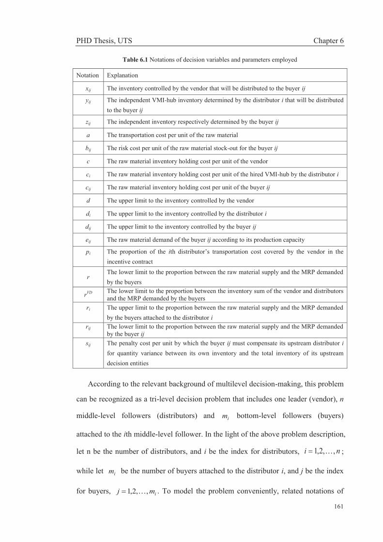
PHD Thesis, UTS Chapter 6
161
Table 6.1 Notations of decision variables and parameters employed
Notation Explanation
xij The inventory controlled by the vendor that will be distributed to the buyer ij
yij The independent VMI-hub inventory determined by the distributor i that will be distributed to the buyer ij
zij The independent inventory respectively determined by the buyer ij
a The transportation cost per unit of the raw material
bij The risk cost per unit of the raw material stock-out for the buyer ij
c The raw material inventory holding cost per unit of the vendor
ci The raw material inventory holding cost per unit of the hired VMI-hub by the distributor i
cij The raw material inventory holding cost per unit of the buyer ij
d The upper limit to the inventory controlled by the vendor
di The upper limit to the inventory controlled by the distributor i
dij The upper limit to the inventory controlled by the buyer ij
eij The raw material demand of the buyer ij according to its production capacity
pi The proportion of the ith distributor’s transportation cost covered by the vendor in the incentive contract
r The lower limit to the proportion between the raw material supply and the MRP demanded by the buyers
rVD The lower limit to the proportion between the inventory sum of the vendor and distributors and the MRP demanded by the buyers
ri The upper limit to the proportion between the raw material supply and the MRP demanded by the buyers attached to the distributor i
rij The lower limit to the proportion between the raw material supply and the MRP demanded by the buyer ij
sij The penalty cost per unit by which the buyer ij must compensate its upstream distributor i for quantity variance between its own inventory and the total inventory of its upstream decision entities
According to the relevant background of multilevel decision-making, this problem
can be recognized as a tri-level decision problem that includes one leader (vendor), n
middle-level followers (distributors) and im bottom-level followers (buyers)
attached to the ith middle-level follower. In the light of the above problem description,
let n be the number of distributors, and i be the index for distributors, ni ,,2,1 ;
while let im be the number of buyers attached to the distributor i, and j be the index
for buyers, imj ,,2,1 . To model the problem conveniently, related notations of

PHD Thesis, UTS Chapter 6
162
decision variables and key parameters in the scenario are shown in Table 6.1. It can
be easily found in Table 6.1 that xij ( ,,,2,1 ni imj ,,2,1 ) are the decision
variables controlled by the vendor; yij ( imj ,,2,1 ) are the decision variables
controlled by the distributor i ( ni ,,2,1 ); and zij is the decision variable controlled
by the buyer ij ( ,,,2,1 ni imj ,,2,1 ). For the sake of convenient argument in
the following sections, let ),,,,,,( 1111 1 nnmnm xxxxx denote the vector of the
vendor's decision variables, whereas let ),,( 1 iimii xyy be the vector of decision
variables controlled by the distributor i for ni ,,2,1 .
6.3 ANALYTICAL MODEL Based on the above problem statement and related notations, the tri-level decision
model for the decentralized VMI coordination scenario is established as follows.
),,,,,,,,,,(min 11111)1(
1 nnmnmnXxzzzzyyxf
n
i
m
jijijijijij
n
i
m
jijiji
n
i
m
jij
iiizyxebzyapxca
1 11 11 1)()()( (Vendor) (6.1a)
s.t. ,)(1 11 1
n
i
m
jij
n
i
m
jijijij
iirezyx (6.1b)
,)(1 11 1
n
i
m
jij
VDn
i
m
jijij
iieryx (6.1c)
,01 1
dxn
i
m
jij
i (6.1d)
where, for each ),,( 1 iimii xxx given, ),,,( 1 iimii zzy solve the problem
(6.1e-6.1j):
),,,,,,(m i n 11
)2(
, iiii
imiiimiiYyzzyxxf
iii m
jijijijij
m
jijiji
m
jiji zyxszypayc
111)()()1( (Distributor i) (6.1e)

PHD Thesis, UTS Chapter 6
163
s.t. ,)(11
ii m
jiji
m
jijijij erzyx (6.1f)
,01
i
m
jij dy
i (6.1g)
where, for each ),( ijij yx given, ijz solves the problem (6.1h-6.1j):
)(),,(min )3(ijijijijijijijijijijZz
zyxszczyxfijij
(Buyer ij) (6.1h)
s.t. ,ijijijijij erzyx (6.1i)
.0 ijij dz (6.1j)
The vendor’s objective function (6.1a) involves the inventory and transportation
cost n
i
m
jij
ixca
1 1)( , the incentive payment
n
i
m
jijiji
izyap
1 1])([ for the distributors’
transportation cost, and the risk cost n
i
m
jijijijijij
izyxeb
1 1)( of stock-out. The
constraint condition (6.1b) implies that the lower limit to the total inventory of the
VMI system must satisfy the proportion r of the raw material demand of all buyers,
which reflects the replenishment policy anticipated by the vendor. (6.1c) implies that
the lower limit to the total inventory of the vendor and the distributors is n
i
m
jij
VDi
er1 1
.
(6.1d) represents the lower and upper limits to the inventory holding capacity of the
vendor.
The objective function (6.1e) of the distributor i involves the raw material
inventory holding cost im
jiji yc
1 of its hired VMI hub, the transportation cost
im
jijiji zypa
1)()1( and the subtractive penalty term
im
jijijijij zyxs
1)( derived
from its downstream buyers’ compensation payments for the inventory variance. The
constraint condition (6.1f) means the replenishment policy anticipated by the
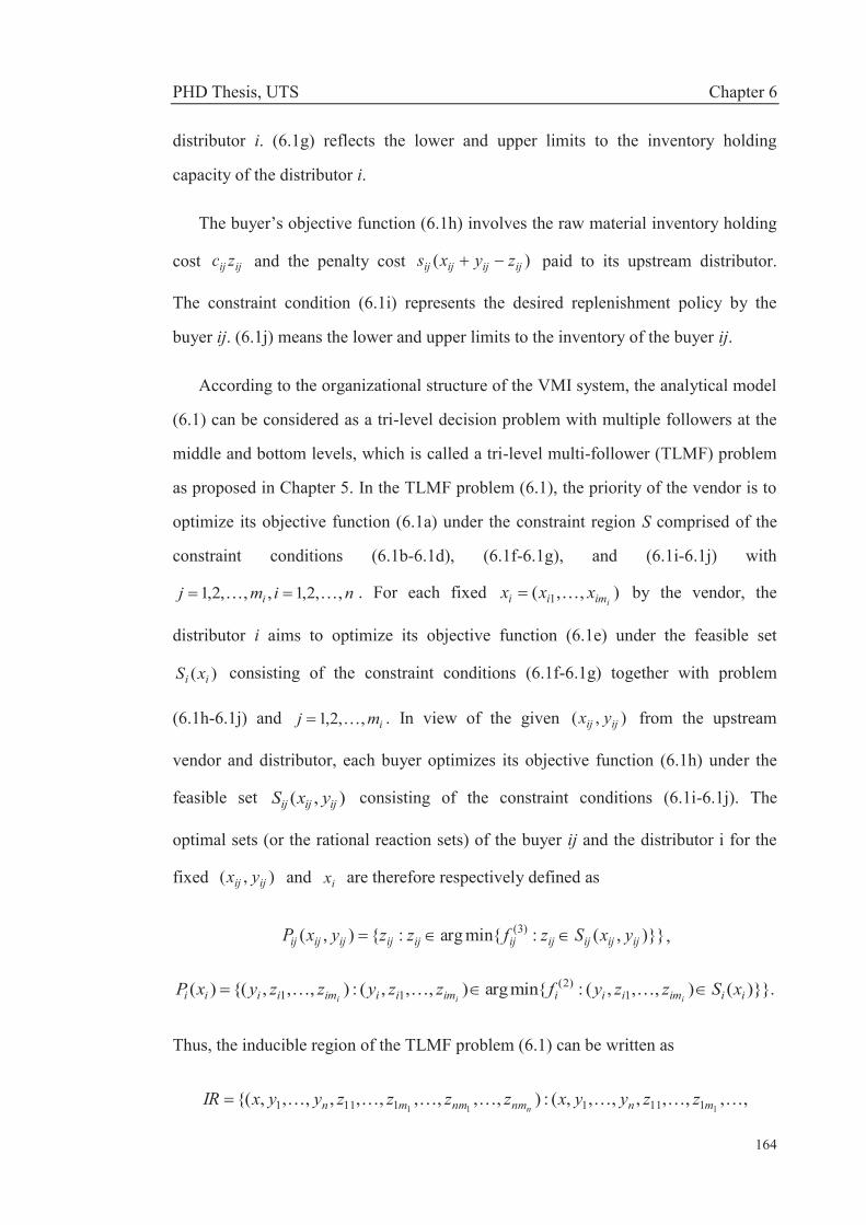
PHD Thesis, UTS Chapter 6
164
distributor i. (6.1g) reflects the lower and upper limits to the inventory holding
capacity of the distributor i.
The buyer’s objective function (6.1h) involves the raw material inventory holding
cost ijij zc and the penalty cost )( ijijijij zyxs paid to its upstream distributor.
The constraint condition (6.1i) represents the desired replenishment policy by the
buyer ij. (6.1j) means the lower and upper limits to the inventory of the buyer ij.
According to the organizational structure of the VMI system, the analytical model
(6.1) can be considered as a tri-level decision problem with multiple followers at the
middle and bottom levels, which is called a tri-level multi-follower (TLMF) problem
as proposed in Chapter 5. In the TLMF problem (6.1), the priority of the vendor is to
optimize its objective function (6.1a) under the constraint region S comprised of the
constraint conditions (6.1b-6.1d), (6.1f-6.1g), and (6.1i-6.1j) with
nimj i ,,2,1,,,2,1 . For each fixed ),,( 1 iimii xxx by the vendor, the
distributor i aims to optimize its objective function (6.1e) under the feasible set
)( ii xS consisting of the constraint conditions (6.1f-6.1g) together with problem
(6.1h-6.1j) and imj ,,2,1 . In view of the given ),( ijij yx from the upstream
vendor and distributor, each buyer optimizes its objective function (6.1h) under the
feasible set ),( ijijij yxS consisting of the constraint conditions (6.1i-6.1j). The
optimal sets (or the rational reaction sets) of the buyer ij and the distributor i for the
fixed ),( ijij yx and ix are therefore respectively defined as
)}},(:min{arg:{),( )3(ijijijijijijijijijij yxSzfzzyxP ,
)}}.(),,,(:min{arg),,,(:),,,{()( 1)2(
11 iiimiiiimiiimiiii xSzzyfzzyzzyxPiii
Thus, the inducible region of the TLMF problem (6.1) can be written as
,,,,,,,,(:),,,,,,,,,,{(111 11111111 mnnmnmmn zzyyxzzzzyyxIR
n
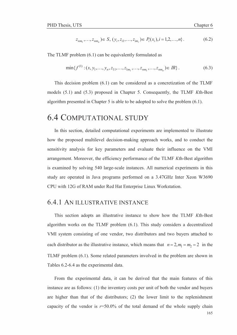
PHD Thesis, UTS Chapter 6
165
,),,1
Szznnmnm },,2,1),(),,,( 1 nixPzzy iiimii i
. (6.2)
The TLMF problem (6.1) can be equivalently formulated as
}),,,,,,,,,,(:min{111111
)1( IRzzzzyyxfnnmnmmn . (6.3)
This decision problem (6.1) can be considered as a concretization of the TLMF
models (5.1) and (5.3) proposed in Chapter 5. Consequently, the TLMF Kth-Best
algorithm presented in Chapter 5 is able to be adopted to solve the problem (6.1).
6.4 COMPUTATIONAL STUDY In this section, detailed computational experiments are implemented to illustrate
how the proposed multilevel decision-making approach works, and to conduct the
sensitivity analysis for key parameters and evaluate their influence on the VMI
arrangement. Moreover, the efficiency performance of the TLMF Kth-Best algorithm
is examined by solving 540 large-scale instances. All numerical experiments in this
study are operated in Java programs performed on a 3.47GHz Inter Xeon W3690
CPU with 12G of RAM under Red Hat Enterprise Linux Workstation.
6.4.1 AN ILLUSTRATIVE INSTANCE
This section adopts an illustrative instance to show how the TLMF Kth-Best
algorithm works on the TLMF problem (6.1). This study considers a decentralized
VMI system consisting of one vendor, two distributors and two buyers attached to
each distributor as the illustrative instance, which means that 2,2 21 mmn in the
TLMF problem (6.1). Some related parameters involved in the problem are shown in
Tables 6.2-6.4 as the experimental data.
From the experimental data, it can be derived that the main features of this
instance are as follows: (1) the inventory costs per unit of both the vendor and buyers
are higher than that of the distributors; (2) the lower limit to the replenishment
capacity of the vendor is r=50.0% of the total demand of the whole supply chain

PHD Thesis, UTS Chapter 6
166
network; (3) the vendor adopts an incentive contract with the first distributor
( %1001p ) while the vendor does not use an incentive contract with the second
distributor ( 02p ); (4) both distributors use a penalty contract with their respective
downstream buyers and the penalty cost ( 50.0ijs ) is much smaller than the
inventory holding cost.
Table 6.2 Data for the vendor
a c d r VDr
1.0 3.0 25 50.0% 35%
Table 6.3 Data for the distributors
i ic id ip ir
1 2.0 50 100% 90.0%
2 2.0 50 0 80.0%
Table 6.4 Data for the buyers
i j ijb ijc ijd ije ijr ijs
1 1 2.0 3.0 10 50 80.0% 0.50
2 2.0 3.0 20 50 80.0% 0.50
2 1 2.0 3.0 10 50 70.0% 0.50
2 2.0 3.0 15 50 70.0% 0.50
The TLMF Kth-Best algorithm is used to solve the problem and the detailed
computing process is shown in Table 6.5 which includes related data and parameters
generated in the computing process. Table 6.5 presents the vertex
),,,,,,( 2221121121kkkkkkkk zzzzyyxs that is searched in the current iteration k, and the
adjacent vertices set kW of the current vertex ks . T represents the set of vertices
that have been searched in past iterations while W is the set of vertices that are
required to verify whether or not an optimal solution occurs inside in the following
iteration. Following the procedures of the TLMF Kth-Best algorithm, an optimal
solution is finally obtained after five iterations. Note that kW in Table 6.5 does not

PHD Thesis, UTS Chapter 6
167
involve the adjacent vertices of ks that have been found in previous iterations and
have been involved in W.
Table 6.5 The detailed computing process of the TLMF Kth-Best algorithm
Iteration k
Vertex sk Wk T W
1 (0,0,0,0,30,20,30,20,10,20,10,15) {(0,0,5,0,30,20,30,20,10,20,10,15), (0,0,0,5,30,20,35,15,10,20,10,15),
(0,0,0,0,30,20,25,20,10,20,10,15), (0,0,0,0,30,20,30,20,10,20,5,15), (0,0,0,0,30,20,25,25,10,20,10,10), (0,0,0,0,30,20,25,25,10,20,10,15)}
{s1} 1W
2 (0,0,0,0,30,20,25,25,10,20,10,15) {(0,0,5,0,30,20,20,30,10,20,10,15), (0,0,0,5,30,20,25,25,10,20,10,15)}
{s1,s2} TWW \)( 2
3 (0,0,5,0,30,20,30,20,10,20,10,15) {(0,0,15,0,30,20,30,20,10,20,0,15), (0,0,20,0,30,20,15,35,10,20,10,0),
(0,0,25,0,30,20,10,20,10,20,10,15)}
{s1,s2,s3} TWW \)( 3
4 (0,0,0,5,30,20,35,15,10,20,10,15) {(0,0,0,15,30,20,45,5,10,20,0,15), (0,0,0,20,30,20,35,0,10,20,10,15),
(0,0,0,20,30,20,35,15,10,20,10,0)}
{s1,s2,s3,s4} TWW \)( 4
5 (0,0,0,0,30,20,25,20,10,20,10,15) --- -- ---
Table 6.6 displays the objective values of all decision entities respectively towards
each solution enumerated by the TLMF Kth-Best algorithm. As it can be seen from
Table 6.6, under the current VMI decision-making context in the supply chain
network, )15,10,20,10,20,30,20,30,0,0,0,0(),,,,,,( 122
121
112
111
12
11
11 zzzzyyxs is the
individual best solution to the vendor, which implies that the vendor anticipates that
the distributors and buyers can choose ,20,10,20,30,20,30(),,,,,( 122
121
112
111
12
11 zzzzyy
)15,10 to respond to the vendor after it has determined x=(0,0,0,0). However, the
distributors and buyers prefer to choose ,10,10,20,25,20,30(),,,,,( 522
521
512
511
52
51 zzzzyy
)15,10 to respond to the vendor to optimize their own objective functions. For the
fixed decision x=(0,0,0,0) by the vendor, )20,30(1y and )20,25(2y are the best
solution for the first and second distributor respectively while considering the implicit

PHD Thesis, UTS Chapter 6
168
reactions of their downstream buyers. In view of the given decision )30,0(),( 1111 yx
and )20,0(),( 1212 yx from the vendor and the first distributor, buyer 11 and buyer
12 achieve an optimal solution )20,10(),( 1211 zz to respond to the vendor and the
first distributor. Similarly, for the given decision )25,0(),( 2121 yx and
)20,0(),( 2222 yx from the vendor and the second distributor, buyer 21 and buyer 22
achieve an optimal solution )15,10(),( 2221 zz to respond to the vendor and the
second distributor. Clearly, )20,10,20,30(),,,( 12111211 zzyy and ),,,( 22212221 zzyy
)15,10,20,25( are the best solutions respectively for the distributor i(i=1,2) and its
buyers to react to the given decision x=(0,0,0,0) by the vendor. Therefore,
)15,10,10,10,20,25,20,30,0,0,0,0(),,,,,,( 522
521
512
511
52
51
5 zzzzyyx is an optimal solution to
the decentralized VMI coordination problem.
Table 6.6 Solutions and objective values of decision entities
Iteration k Vertex sk )1(f )2(1f )2(
2f )3(11f )3(
12f )3(21f )3(
22f
1 (0,0,0,0,30,20,30,20,10,20,10,15) 170.0 90.0 162.5 40.0 60.0 40.0 47.5
2 (0,0,0,0,30,20,25,25,10,20,10,15) 170.0 90.0 162.5 40.0 60.0 37.5 50.0
3 (0,0,5,0,30,20,30,20,10,20,10,15) 180.0 90.0 160.0 40.0 60.0 42.5 47.5
4 (0,0,0,5,30,20,35,15,10,20,10,15) 180.0 90.0 160.0 40.0 60.0 42.5 47.5
5 (0,0,0,0,30,20,25,20,10,20,10,15) 180.0 90.0 150.0 40.0 60.0 37.5 47.5
Although the vendor’s total cost has become worse by increasing from 170.0 to
180.0 during the decision process from 1s to 5s , the vendor cannot obtain a better
objective value by moving away from the vertex over the IR, because some
individuals try to obtain better results for themselves under the VMI coordination,
yielding the solution 5s . Therefore, the vertex 5s is an optimal solution to the VMI
planning problem, which means a final coordinated result for decision entities in the
current VMI decision context. The coordinated result indicates that the vendor may
not achieve its individual optimal solution under the constraint region even though it

PHD Thesis, UTS Chapter 6
169
has priority in making decisions, since its decisions are implicitly determined by
reactions of its downstream decision entities. Clearly, the TLMF Kth-Best algorithm
provides a practical way to solve the TLMF optimization problem (6.1). The optimal
solution to the TLMF problem (6.1) means a compromised equilibrium under VMI
coordination.
6.4.2 SENSITIVITY ANALYSIS
In this section, the sensitivity analysis is conducted for key parameters of the VMI
system involving the distributor’s and buyer's inventory upper limits, the distributor’s
transportation cost, and the incentive and penalty mechanism. This section analyzes
their influence on the coordinated VMI results and the individual performance of each
decision entity.
6.4.2.1 EFFECT OF THE DISTRIBUTOR’S AND BUYER'S
INVENTORY UPPER LIMITS
This section conducts one group of numerical experiments to analyze the effect of
the distributor’s and buyer's inventory upper limits on the VMI performance while
considering the illustrative instance in Section 6.4.1 as the base problem. Under VMI
coordination, with the upper limits to the first distributor’s inventory and its first
buyer's inventory respectively increasing from 30 to 60 and decreasing from 10 to 0,
the corresponding optimal solutions and coordinated results are given in Table 6.7.
It can be seen from Table 6.7 that the vendor prefers to reduce its own inventory
when the distributor's inventory upper limit increases under certain inventory upper
limit of the buyers. The cost of the distributor increases while that of the vendor
declines during the period. The much higher upper limit to the distributor’s inventory
will not result in an extended reduction of the vendor’s inventory until the vendor's
inventory equals to zero. Table 6.7 also shows that the distributor will increase its
inventory level following the decrease in its downstream buyer's inventory upper limit.
PHD Thesis, UTS Chapter 6
170
After the distributor's inventory upper limit is full filled, the vendor will keep higher
inventory level to maintain the raw material supply for the buyer. The buyer's cost
experiences a downward trend following the decrease in its own inventory, while that
of the vendor grows gradually. However, the experiment is performed in which the
number 11d is set smaller than 5 under 301d such that an optimal solution to the
TLMF problem (6.1) cannot be found, which implies that the much smaller upper
limit to the buyer's inventory is not permitted in the VMI system if the vendor and the
distributor do not possess sufficient inventory upper limit. In contrast, it is noticeable
in case 10 that, if the distributor’s inventory upper limit is large enough, both the
vendor and the buyer are able to reduce their own inventory level to zero; meanwhile,
their costs both decreases. Thus, for the sake of achieving zero inventory, the vendor
and buyers, as the manufacturing enterprises, should try to persuade the distributors to
improve their individual inventory upper limits when making the VMI contract.

PHD Thesis, UTS Chapter 6
171
Table 6.7 The experimental results based on the distributor’s and buyer's inventory upper limits changes
Experiments The optimal solutions and coordinated results Computational performance
Case d1 d11 ),,,,,,( 2221121121 zzzzyyx )1(f )2(1f )2(
2f )3(11f )3(
12f )3(21f )3(
22f Iteration Time (s)
1 30 10 (0,20,0,0,30,0,25,20,10,20,10,15) 240.0 50.0 150.0 40.0 60.0 37.5 47.5 6 0.221
2 5 (5,20,0,0,30,0,25,20,5,20,10,15) 255.0 45.0 150.0 30.0 60.0 37.5 47.5 5 0.159
3 0 Not Applicable 0 0.015
4 40 10 (0,10,0,0,30,10,25,20,10,20,10,15) 210.0 70.0 150.0 40.0 60.0 37.5 47.5 7 0.236
5 5 (0,15,0,0,35,5,25,20,5,20,10,15) 225.0 65.0 150.0 30.0 60.0 37.5 47.5 8 0. 251
6 0 (0,20,0,0,40,0,25,20,0,20,10,15) 240.0 60.0 150.0 20.0 60.0 37.5 47.5 6 0.189
7 50 10 (0,0,0,0,30,20,25,20,10,20,10,15) 180.0 90.0 150.0 40.0 60.0 37.5 47.5 5 0.144
8 5 (0,5,0,0,35,15,25,20,5,20,10,15) 195.0 85.0 150.0 30.0 60.0 37.5 47.5 7 0.236
9 0 (0,10,0,0,40,10,25,20,0,20,10,15) 210.0 80.0 150.0 20.0 60.0 37.5 47.5 7 0.235
10 60 10 (0,0,0,0,30,20,25,20,10,20,10,15) 180.0 90.0 150.0 40.0 60.0 37.5 47.5 7 0.285
11 5 (0,0,0,0,35,20,25,20,5,20,10,15) 180.0 95.0 150.0 30.0 60.0 37.5 47.5 7 0.208
12 0 (0,0,0,0,40,20,25,20,0,20,10,15) 180.0 100.0 150.0 20.0 60.0 37.5 47.5 7 0.220

PHD Thesis, UTS Chapter 6
172
6.4.2.2 EFFECT OF THE PENALTY MECHANISM
To identify the effect of the penalty mechanism between each distributor and its
downstream buyers, this section analyzes the coordinated results for the penalty cost
of the second buyer attached to the second distributor (called buyer 22) increasing
from 0 to 4.0. The experimental results, which consider case 7 in the above section as
the basic problem, are shown in Table 6.8.
As shown in Table 6.8, when the penalty cost is smaller (e.g. 022s , 5.022s
and 0.122s ), the second distributor’s cost amounts is higher in value. In this
situation, the second distributor does not prefer to increase its inventory level and
buyer 22 has to keep a certain amount of back-up inventory to service the production
demand. With the penalty cost increasing from 1.5 to 3.0, the second distributor is
willing to increase its inventory to its upper limit to reduce its total cost while the
buyer 22 need not to keep so many inventory but has to compensate the higher
penalty cost for the second distributor. However, when the penalty cost is higher than
the inventory cost (e.g. 5.322s and 0.422s ), buyer 22 will increase its holding
inventory to reduce the penalty cost, even though the second distributor prefers to
hold the largest inventory. Table 6.8 also clearly shows that the total cost of the
second distributor reaches the bottom when the penalty cost is equal to the inventory
cost. Thus, the second distributor can price the penalty cost at 0.322s in designing
the penalty VMI contract with the buyer. During the same period, the vendor's cost
decreases from 180.0 to 170.0, which means that the vendor can persuade distributors
to increase the penalty cost with the buyers in order to motivate the buyers to hold
more inventory if the vendor seeks to improve its individual performance.

PHD Thesis, UTS Chapter 6
173
Table 6.8 The experimental results based on the penalty cost changes
Experiments The optimal solutions and coordinated results Computational performance
Case s22 ),,,,,,( 2221121121 zzzzyyx )1(f )2(1f )2(
2f )3(11f )3(
12f )3(21f )3(
22f Iteration Time (s)
13 0 (0,0,0,0,30,20,25,20,10,20,10,15) 180.0 90.0 152.5 40.0 60.0 37.5 45.0 5 0.149
7 0.5 (0,0,0,0,30,20,25,20,10,20,10,15) 180.0 90.0 150.0 40.0 60.0 37.5 47.5 5 0.144
14 1.0 (0,0,0,0,30,20,25,20,10,20,10,15) 180.0 90.0 147.5 40.0 60.0 37.5 50.0 5 0.143
15 1.5 (0,0,0,0,30,20,25,25,10,20,10,10) 180.0 90.0 140.0 40.0 60.0 37.5 52.5 7 0.221
16 2.0 (0,0,0,0,30,20,25,25,10,20,10,10) 180.0 90.0 132.5 40.0 60.0 37.5 60.0 7 0.212
17 2.5 (0,0,0,0,30,20,25,25,10,20,10,10) 180.0 90.0 125.0 40.0 60.0 37.5 67.5 7 0.225
18 3.0 (0,0,0,0,30,20,25,25,10,20,10,10) 180.0 90.0 117.5 40.0 60.0 37.5 75.0 7 0.220
19 3.5 (0,0,0,0,30,20,25,25,10,20,10,15) 170.0 90.0 132.5 40.0 60.0 37.5 80.0 2 0.063
20 4.0 (0,0,0,0,30,20,25,25,10,20,10,15) 170.0 90.0 127.5 40.0 60.0 37.5 85.0 2 0.047

PHD Thesis, UTS Chapter 6
174
Table 6.9 The experimental results based on the distributor’s transportation cost changes
Experiments The optimal solutions and coordinated results Computational performance
Case p2 a ),,,,,,( 2221121121 zzzzyyx )1(f )2(1f )2(
2f )3(11f )3(
12f )3(21f )3(
22f Iteration Time (s)
17 0 1.0 (0,0,0,0,30,20,25,25,10,20,10,10) 180.0 90.0 125.0 40.0 60.0 37.5 67.5 7 0.225
21 1.5 (0,0,0,0,30,20,25,20,10,20,10,15) 220.0 90.0 160.0 40.0 60.0 37.5 67.5 5 0.159
22 2.0 (0,0,0,0,30,20,25,20,10,20,10,15) 260.0 90.0 195.0 40.0 60.0 37.5 67.5 5 0.172
23 2.5 (0,0,0,0,30,20,25,20,10,20,10,15) 300.0 90.0 230.0 40.0 60.0 37.5 67.5 5 0.126
24 100% 1.0 (0,0,0,0,30,20,25,25,10,20,10,10) 250.0 90.0 55.0 40.0 60.0 37.5 67.5 5 0. 134
25 1.5 (0,0,0,0,30,20,25,25,10,20,10,10) 325.0 90.0 55.0 40.0 60.0 37.5 67.5 5 0.141
26 2.0 (0,0,0,0,30,20,25,25,10,20,10,10) 400.0 90.0 55.0 40.0 60.0 37.5 67.5 3 0.078
27 2.5 (0,0,0,0,30,20,25,25,10,20,10,10) 475.0 90.0 55.0 40.0 60.0 37.5 67.5 3 0.078
PHD Thesis, UTS Chapter 6
175
6.4.2.3 EFFECT OF THE TRANSPORTATION COST AND THE
INCENTIVE MECHANISM
In this section, case 17 is considered as the basic problem based on the related
discussion in Section 6.4.2.2 to ensure that the reaction space of the distributors is
well positioned. The experimental results for the transportation cost ranging from 1.0
to 2.5 are reported in Table 6.9 and can be classified into two groups according to
whether or not the incentive mechanism by 02p and %1002p is considered
between the vendor and the second distributor.
The obtained results in Table 6.9 without considering the incentive mechanism
( 02p ) show that, when the transportation cost is increased, the second distributor's
inventory decreases during the same period while the inventory of buyer 22 increases.
Since the buyer will react to the decrease in the second distributor’s inventory by
improving its own inventory level, the second distributor anticipates the reduction in
its transportation cost by reducing its own inventory level. In contrast, when the
incentive contract is considered ( %0102p ), the inventory of the second distributor
remains stable at a higher level. The results imply that the increase in the
transportation cost results in the inventory reduction of the distributor when the
incentive contract is not considered.
Table 6.9 reports that the vendor’s and the second distributor’s costs respectively
experience an upward trend without the incentive mechanism, while the first
distributor’s cost remains stable at 90.0 because of the incentive mechanism. When
the incentive contract is considered, the total cost of the vendor is higher than the
same number under 02p , while the second distributor’s cost becomes smaller than
the same number under 02p . In addition, following the transportation cost
increasing under %1002p , the cost of the second distributor remains stable as does

PHD Thesis, UTS Chapter 6
176
that of the first distributor, and only the total cost of the vendor increases. The above
analysis reflects that the incentive mechanism contributes to a better individual
performance of the distributor during the period that the transportation cost rises up,
thus, the vendor can use a incentive contract to encourage the distributor to keep more
inventory for maintaining the raw material supply following the increase in the
transportation cost. The results also imply that the upstream decision entities should
take into account the implicit reactions of its downstream decision entities when
making its own decisions under VMI coordination.
6.4.3 ASSESSING THE EFFICIENCY PERFORMANCE OF
THE TLMF KTH-BEST ALGORITHM
The experimental results in Tables 6.7-6.9 show that very little computing time is
spent on solving each experimental case, which implies that the TLMF Kth-Best
algorithm can be carried out efficiently. However, those previously mentioned cases
1-27 are considered as small-scale instances. The efficiency performance of the
algorithm may declines rapidly with the increase in the mass of distributors and
buyers. To assess the algorithm performance in depth, the proposed TLMF Kth-Best
algorithm is used to solve large-scale instances in this section.
The TLMF decision techniques for modeling decentralized VMI coordination
problem have not been considered in literatures, therefore, there are no benchmark
instances. In this study, large-scale instances are randomly generated to cover a wide
range of problem structures based on the sensitivity analysis in Section 6.4.2. The test
instances are classified into 18 different problem sets following the number of
distributors and buyers becoming larger and larger, which are displayed in Table 6.10.
As shown in Table 6.10, n and m are the number of distributors and buyers
respectively, whereas the number (mi) of buyers that are attached to the same
distributor i ( ni ,,2,1 ) is randomly determined under mmn
ii
1 and 0im .
Table 6.10 also shows the numbers of decision variables and constraint conditions,

PHD Thesis, UTS Chapter 6
177
respectively known as Num(v) and Num(con). It can be seen from model (6.1) that
Num(v) is determined by the number of buyers, whereas Num(con) is determined by
the total number of distributors and buyers. In this computational study, 30 test
problems are randomly constructed within each problem set; thus, there are
5401830 different instances randomly generated as a whole within 18 test
problem sets.
Table 6.10 Test instances randomly generated
Problem set n m Num(v) Num(con) Problem set n m Num(v) Num(con)
P01 2 8 24 23 P10 10 30 90 83
P02 4 8 24 27 P11 15 30 90 93
P03 6 8 24 31 P12 20 30 90 103
P04 4 15 45 41 P13 15 40 120 113
P05 6 15 45 45 P14 20 40 120 123
P06 10 15 45 53 P15 30 40 120 143
P07 6 20 60 55 P16 20 50 150 143
P08 10 20 60 63 P17 30 50 150 163
P09 15 20 60 73 P18 50 50 150 203
In terms of parameters in model (6.1), buyer demand eij is randomly chosen from
the uniform distribution on [40, 60], and buyer inventory upper limit dij is generated
from uniform random numbers between 5 and 20. For the sake of ensuring the
problem is well posed, distributor inventory upper limit di is randomly chosen from
the interval ]10)(,10)([11
ii m
jijijij
m
jijijij dredre , whereas vendor inventory upper
limit d is uniformly distributed on ]10))((,))(([,1 1,1 1
n
siii
m
jijijij
n
siii
m
jijijij ddreddre
ii
where 0)(1
s
m
jsjsjsj ddre
s. The remainder parameters in model (6.1) keep the
same as those in Section 6.4.1 apart from setting %100ip , %90ir , %80ijr
and 5.1ijs .

PHD Thesis, UTS Chapter 6
178
Table 6.11 The experimental results of the randomly generated test problems
Problem set n-m-Num(v)-Num(con) Num(best) Iteration Time (s) Problem set n-m-Num(v)-Num(con) Num(best) Iteration Time (s)
P01 2-8-24-23 30 17.77 17.953 P10 10-30-90-83 27 579.52 387.541
P02 4-8-24-27 30 36.57 23.117 P11 15-30-90-93 26 558.81 401.259
P03 6-8-24-31 30 32.50 24.812 P12 20-30-90-103 27 564.67 431.524
P04 4-15-45-41 30 147.27 39.798 P13 15-40-120-113 22 768.82 694.258
P05 6-15-45-45 30 196.40 57.814 P14 20-40-120-123 20 737.05 729.654
P06 10-15-45-53 30 164.53 65.237 P15 30-40-120-143 24 727.50 758.216
P07 6-20-60-55 29 491.69 185.642 P16 20-50-150-143 19 873.53 991.852
P08 10-20-60-63 28 427.82 208.858 P17 30-50-150-163 22 843.45 1036.248
P09 15-20-60-73 30 383.23 221.341 P18 50-50-150-203 18 819.00 1123.982

PHD Thesis, UTS Chapter 6
179
The TLMF Kth-Best algorithm is used to solve these 540 test problems randomly
generated. In terms of solving each problem, the maximal iteration number is 1000
and each problem is carried out 10 runs to collect the computing CPU time. If the
algorithm can find an optimal solution for a problem within 1000 iterations, it is
considered as successful computation. Table 6.11 shows the number of test problems
successfully solved within each problem set, denoted by Num(best). Table 6.11 also
displays the average of the iteration number and the computing CPU time (in seconds)
for each problem set.
It is clear in Table 6.11 that the number of problems successfully solved becomes
smaller following the increase in the number of distributors and buyers. The reason is
that more and more test problems have no solutions or the computational iterations
exceeds 1000 during the experimental process. To explore more in depth, the
algorithm efficiency is examined, shown as the iterations and computing time in
Table 6.11. As shown in Table 6.11, both the number of iterations and computing
time experience a sharp rise with the problem size being larger and larger. Notice that,
when the number of buyers remains stable, the number of problems successfully
solved, as well as the algorithm efficiency, does not shows substantial change with the
number of distributors increasing. Thus, the number of buyers has a significant
influence on the performance of the TLMF Kth-Best algorithm; Figure 6.2 displays
much more evident results. The results mean that the number of decision variables,
rather than constraint conditions, determines the characteristics of the TLMF problem
(6.1) and the efficiency performance of the TLMF Kth-Best algorithm.
Since the TLMF problems have not been solved by other algorithms in literatures,
the algorithm performance cannot be compared with others. In this study, the
efficiency performance of the TLMF Kth-Best algorithm is assessed using the growth
trend of the computing CPU time for solving these test problems. It can be found in
Figure 6.3 that the growth trend of CPU time coincides with a fitted quadratic
polynomial curve rather than a exponential curve. Clearly, although the computational
load of the TLMF Kth-Best experiences a steep upward trend in response to the

PHD Thesis, UTS Chapter 6
180
problem size becoming larger, these test problems can be solved by the algorithm in a
quadratic polynomial time, which is a reasonable computing time for solving NP-hard
problems. Therefore, the TLMF Kth-Best algorithm can be considered as a feasible
and an effective approach for solving the proposed decentralized VMI coordination
problems.
Figure 6.2 The average of iterations and CPU time for solving the test problems
Figure 6.3 The fitted curve of CPU time following the number of buyers change
0
200
400
600
800
1000
1200
1400
0100200300400500600700800900
1000
P01 P02 P03 P04 P05 P06 P07 P08 P09 P10 P11 P12 P13 P14 P15 P16 P17 P18
CPU
tim
e
Itera
tions
Problem set
Iterations CPU time
Time = 0.3251m2 + 6.4138m - 71.394
Time = 17.211e0.0911m
0200400600800
10001200140016001800
0 10 20 30 40 50 60
CPU
tim
e
Number of buyers (m)
CPU time Polynomial curve Exponential curve
PHD Thesis, UTS Chapter 6
181
6.5 SUMMARY This chapter considers a decentralized VMI coordination problem in a
three-echelon hierarchical supply chain network consisting of a vendor, multiple
third-party logistics companies as distributors, and multiple buyers. To deal with the
inventory coordination among the decision entities, this chapter first proposes a linear
TLMF decision model to describe the VMI problem. The TLMF Kth-Best algorithm
developed in Chapter 5 is then used to solve the resulting TLMF decision model. The
sensitivity analysis for key VMI parameters is conducted to examine the operations
multilevel decision-making process in which decision entities coordinate with one
another on the decentralized VMI.
The computational results imply that an optimal solution to the proposed VMI
problem results in a compromised equilibrium for decision entities under inventory
coordination; it may not be the best solution in respect to the vendor, although it has
priority in making decisions. The sensitivity analysis reports that decision entities can
achieve different coordinated results by adjusting related VMI parameters, which
have different influences on the individual performance of each decision entity. The
experimental results also clearly show that the performance improvement of one
individual does not mean the cost reduction of all decision entities, which implies that
decision entities are only concerned with their own cost reduction rather than the
performance improvement of others under VMI coordination. Under VMI
coordination, decision entities should prefer to cooperate with one another in
designing a VMI contract, if they seek to improve their individual performances; for
example, the vendor may persuade distributors to increase their inventory upper limits
to improve the VMI performance, as well, the incentive and penalty mechanism can
be adopted to balance the total cost sharing between decision entities. Moreover, the
computational study shows that large-scale problems can be solved in a reasonable
computing time using the proposed TLMF Kth-Best algorithm.

PHD Thesis, UTS Chapter 6
182
In conclusion, this chapter provides a practical way to handle the decentralized
VMI coordination problem in a three-echelon supply chain network. This chapter
shows how to improve the individual performance of each decision entity and balance
the total cost sharing in a decentralized VMI hierarchy. Of particular importance, this
chapter displays how to design a manufacturer-manufacturer (vendor-buyer) VMI
system where third-party logistics are involved, and through which the vendor and
buyers can achieve their holding inventory as small as possible or even at zero
inventory.
PHD Thesis, UTS Chapter 7
183
CHAPTER 7 CONCLUSIONS AND
FURTHER STUDY
This chapter concludes the whole thesis and provides some further research
directions for the topic.
7.1 CONCLUSIONS Multilevel decision-making techniques have been widely applied to handle
decentralized decision problems in the real world. The latest developments of
multilevel decision-making typically display three features: (1) large-scale -
high-dimensional decision variables make multilevel decision problems large-scale;
(2) uncertainty - uncertain information is always involved in related decision
parameters and conditions, which become imprecisely or ambiguously known to
decision entities; (3) diversification - there may exist multiple decision entities at each
decision level, in which multiple decision entities at the same level have a variety of
relationships with one another. To support large-scale, uncertain and diversified
multilevel decision-making, this research develops related decision models and/or
solution approaches to handle three categories of unsolved multilevel decision
problems, involving large-scale nonlinear bi-level and tri-level decision problems,
fuzzy nonlinear bi-level decision problems and TLMF decision problems. Moreover,
these proposed multilevel decision-making techniques are applied to deal with
decentralized production and inventory operational problems in SCM.
The main contributions of this study are as follows:
PHD Thesis, UTS Chapter 7
184
1) It proposes a bi-level PSO algorithm to solve large-scale nonlinear bi-level
decision problems; the bi-level PSO algorithm is then extended to a tri-level PSO
algorithm for solving tri-level decision problems. (To achieve Objective 1)
In the proposed bi-level/tri-level PSO algorithms, the leader's problem and the
follower's problem are separated based on related solution concepts for convenient
solving. To handle the complexity of the constraint region of nonlinear and
large-scale problems, two methods for constructing the initial population are given.
Moreover, the decreasing inertia weight with time is used to control the velocity of
particles in the search space at different stages, which can improve both the search
and convergence abilities of the bi-level/tri-level PSO algorithms. The computational
results report that the bi-level/tri-level PSO algorithms are able to find much better
solutions than other algorithms and show much better performance in terms of
efficiency than other algorithms which follow the problem size by becoming larger
and larger. Consequently, the proposed bi-level PSO algorithm provides a practical
way to solve large-scale nonlinear bi-level decision problems; moreover, it can be
extended to a tri-level PSO algorithm for solving tri-level decision problems.
2) It proposes a compromise-based PSO algorithm for solving fuzzy nonlinear
bi-level decision problems. (To achieve Objective 2)
The compromise-based PSO algorithm can be used to solve nonlinear bi-level
decision problems with general fuzzy numbers. With regard to the compromise-based
PSO algorithm, the leader and follower can choose acceptable decision conditions
based on rules of compromise due to uncertain decision environments, which can
result in the preferred solution under individual decision situations. The
computational results show that the compromise-based PSO algorithm can not only
provide better solutions to the specific decision situation compared with the existing
solution approaches but also present different options in terms of solutions due to
uncertain decision environments.
PHD Thesis, UTS Chapter 7
185
3) It proposes different TLMF decision models to describe various relationships
between multiple followers at the same level, and discusses theoretical properties
in relation to the existence and optimality of solutions. (To achieve Objective 3)
The TLMF decision models can be applied to describe different decision-making
processes motivated by various relationships between multiple followers at the same
level. Related solution concepts analyze the operations of the TLMF decision-making
process. The theoretical properties give sufficient conditions for the optimal solution
existence and the geometry of the solution space, which provides the theoretical
foundation for designing an effective solution algorithm for solving TLMF decision
problems.
4) It proposes a TLMF Kth-Best algorithm for solving TLMF decision problems and
a evaluation method to assess the solution obtained. (To achieve Objective 4)
The TLMF Kth-Best algorithm ranks the vertices of the constraint region by the
leader's objective value and verifies these vertices in sequence whether or not each
vertex is an optimal solution. The algorithm is not terminated until the Kth vertex is
found that can be considered as an optimal solution. This algorithm can find an
optimal solution to TLMF decision problems; moreover, it is able to solve large-scale
problems in a reasonable and an acceptable time. The TLMF Kth-Best algorithm
overcomes the lack of solution algorithms for solving TLMF decision problems.
Since it is imprecise or ambiguous for decision entities to identify a solution whether
or not they desire it, the solution evaluation method can assess the satisfaction of
decision entities by transforming the objective functions into fuzzy goals. The
solution evaluation method, as a relative criterion, can be applied to analyze how the
TLMF decision-making process varies with changing decision externalities and
provide decision support for decision entities.
5) It applies multilevel decision-making techniques to handle a decentralized VMI
coordination problem in SCM. (To achieve Objective 5)

PHD Thesis, UTS Chapter 7
186
The decentralized VMI coordination problem is modeled as a TLMF decision
problem, which examines how the decision entities coordinate with each other on the
decentralized VMI. The TLMF Kth-Best algorithm developed in Chapter 5 is then
used to solve the resulting TLMF decision model. The computational results indicate
that this research provides a practical way to handle the decentralized VMI
coordination problem in a three-echelon supply chain network. This research shows
how to improve the individual performance of each decision entity and balance the
total cost sharing in a decentralized VMI hierarchy. Even more important, this
research displays how to design a manufacturer-manufacturer (vendor-buyer) VMI
system where third-party logistics are involved, and through which the vendor and
buyers can achieve their holding inventory as low as possible or even at zero
inventory.
7.2 FURTHER STUDY There are still some limitations in relation to the current study:
1) Many multilevel decision problems may have no optimal solutions based on
existing solution concepts. How to find a usable or satisfactory solution to these
multilevel decision problems is an emerging research topic with respect to
computational complexity.
2) The fully fuzzy bi-level decision problems, in which both coefficients and
variables are characterized by fuzzy numbers, is also an emerging research topic
and need to be examined in depth.
3) Multilevel decision problems nowadays often appear in highly complex and
diversified decision environments where decision makers sometimes need to make
an optimal or a wise decision from big data with uncertainty. This requires further
research on how to wisely model such problems and implement data-driven
decision-making in the current age of big data by means of a multilevel decision
support system.

PHD Thesis, UTS Chapter 7
187
4) Multilevel decision-making techniques are mainly limited to mathematical
programming modeling and solving. However, many multilevel decision
problems in the real world cannot be modeled as mathematical programming
formulations. It is another challenge to break through mathematical programs and
integrate the principle of multilevel decision-making with other decision-making
techniques to handle a much wider range of decision problems.

PHD Thesis, UTS References
188
REFERENCES
Aguezzoul, A. 2014, 'Third-party logistics selection problem: A literature review on
criteria and methods', Omega, vol. 49, no. 0, pp. 69-78.
Al-Khayyal, F., Horst, R. & Pardalos, P. 1992, 'Global optimization of concave
functions subject to quadratic constraints: An application in nonlinear bilevel
programming', Annals of Operations Research, vol. 34, no. 1, pp. 125-47.
Alguacil, N., Delgadillo, A. & Arroyo, J.M. 2014, 'A trilevel programming approach
for electric grid defense planning', Computers & Operations Research, vol. 41,
no. 0, pp. 282-90.
Alves, M.J. & Costa, J.P. 2014, 'An algorithm based on particle swarm optimization
for multiobjective bilevel linear problems', Applied Mathematics and
Computation, vol. 247, no. 0, pp. 547-61.
Anandalingam, G. 1988, 'A mathematical programming model of decentralized
multi-level systems', Journal of the Operational Research Society, vol. 39, no.
11, pp. 1021-33.
Anandalingam, G. & Apprey, V. 1991, 'Multi-level programming and conflict
resolution', European Journal of Operational Research, vol. 51, no. 2, pp.
233-47.
Anandalingam, G. & White, D.J. 1990, 'A solution method for the linear static
Stackelberg problem using penalty functions', IEEE Transactions on
Automatic Control, vol. 35, no. 10, pp. 1170-3.
PHD Thesis, UTS References
189
Angulo, E., Castillo, E., García-Ródenas, R. & Sánchez-Vizcaíno, J. 2014, 'A
continuous bi-level model for the expansion of highway networks', Computers
& Operations Research, vol. 41, no. 0, pp. 262-76.
Ankhili, Z. & Mansouri, A. 2009, 'An exact penalty on bilevel programs with linear
vector optimization lower level', European Journal of Operational Research,
vol. 197, no. 1, pp. 36-41.
Apivatanagul, P., Davidson, R. & Nozick, L. 2012, 'Bi-level optimization for
risk-based regional hurricane evacuation planning', Natural Hazards, vol. 60,
no. 2, pp. 567-88.
Arora, S.R. & Gupta, R. 2009, 'Interactive fuzzy goal programming approach for
bilevel programming problem', European Journal of Operational Research,
vol. 194, no. 2, pp. 368-76.
Askin, R.G., Baffo, I. & Xia, M. 2014, 'Multi-commodity warehouse location and
distribution planning with inventory consideration', International Journal of
Production Research, vol. 52, no. 7, pp. 1897-910.
Audet, C., Haddad, J. & Savard, G. 2007, 'Disjunctive cuts for continuous linear
bilevel programming', Optimization Letters, vol. 1, no. 3, pp. 259-67.
Audet, C., Savard, G. & Zghal, W. 2007, 'New Branch-and-Cut Algorithm for Bilevel
Linear Programming', Journal of Optimization Theory and Applications, vol.
134, no. 2, pp. 353-70.
Aviso, K.B., Tan, R.R., Culaba, A.B. & Cruz Jr, J.B. 2010, 'Bi-level fuzzy
optimization approach for water exchange in eco-industrial parks', Process
Safety & Environmental Protection: Transactions of the Institution of
Chemical Engineers Part B, vol. 88, no. 1, pp. 31-40.
Bard, J. 1988, 'Convex two-level optimization', Mathematical Programming, vol. 40,
PHD Thesis, UTS References
190
no. 1-3, pp. 15-27.
Bard, J.F. 1984, 'An investigation of the linear three level programming problem',
IEEE Transactions on Systems, Man, and Cybernetics, vol. SMC-14, no. 5, pp.
711-7.
Bard, J.F. 1991, 'Some properties of the bilevel programming problem', Journal of
Optimization Theory and Applications, vol. 68, no. 2, pp. 371-8.
Bard, J.F. 1998, Practical Bilevel Optimization: Algorithms and Applications, Kluwer
Academic Publishers, Dordrecht, The Netherlands.
Bard, J.F. & Falk, J.E. 1982, 'An explicit solution to the multi-level programming
problem', Computers & Operations Research, vol. 9, no. 1, pp. 77-100.
Bard, J.F. & Moore, J.T. 1990, 'A branch and bound algorithm for the bilevel
programming problem', SIAM Journal on Scientific and Statistical Computing,
vol. 11, no. 2, pp. 281-92.
Bard, J.F. & Moore, J.T. 1992, 'An algorithm for the discrete bilevel programming
problem', Naval Research Logistics (NRL), vol. 39, no. 3, pp. 419-35.
Ben-Aved, O. & Blair, C.E. 1990, 'Computational difficulties of bilevel linear
programming', Operations Research, vol. 38, no. 3, pp. 556-60.
Berling, P. & Marklund, J. 2014, 'Multi-echelon inventory control: an adjusted normal
demand model for implementation in practice', International Journal of
Production Research, pp. 1-17.
Bialas, W. & Karwan, M.H. 1984, 'Two-level linear programming', Management
Science, vol. 30, pp. 1004-20.
Bianco, L., Caramia, M. & Giordani, S. 2009, 'A bilevel flow model for hazmat
transportation network design', Transportation Research Part C: Emerging

PHD Thesis, UTS References
191
Technologies, vol. 17, no. 2, pp. 175-96.
Budnitzki, A. 2013, 'The solution approach to linear fuzzy bilevel optimization
problems', Optimization, pp. 1-15.
Calvete, H.I. & Galé, C. 2007, 'Linear bilevel multi-follower programming with
independent followers', Journal of Global Optimization, vol. 39, no. 3, pp.
409-17.
Calvete, H.I. & Galé, C. 2010, 'Linear bilevel programs with multiple objectives at
the upper level', Journal of Computational and Applied Mathematics, vol. 234,
no. 4, pp. 950-9.
Calvete, H.I. & Galé, C. 2011, 'On linear bilevel problems with multiple objectives at
the lower level', Omega, vol. 39, no. 1, pp. 33-40.
Calvete, H.I. & Galé, C. 2012, 'Linear bilevel programming with interval coefficients',
Journal of Computational and Applied Mathematics, vol. 236, no. 15, pp.
3751-62.
Calvete, H.I., Galé, C. & Iranzo, J.A. 2014, 'Planning of a decentralized distribution
network using bilevel optimization', Omega, vol. 49, no. 0, pp. 30-41.
Calvete, H.I., Galé, C. & Mateo, P.M. 2008, 'A new approach for solving linear
bilevel problems using genetic algorithms', European Journal of Operational
Research, vol. 188, no. 1, pp. 14-28.
Calvete, H.I., Galé, C. & Oliveros, M.-J. 2011, 'Bilevel model for
production–distribution planning solved by using ant colony optimization',
Computers & Operations Research, vol. 38, no. 1, pp. 320-7.
Calvete, H.I., Galee, C. & Mateo, P.M. 2008, 'A new approach for solving linear
bilevel problems using genetic algorithms', European Journal of Operational
Research, vol. 188, no. 1, pp. 14-28.

PHD Thesis, UTS References
192
Camacho-Vallejo, J.-F., González-Rodríguez, E., Almaguer, F.J. & González-Ramírez,
R.G. 2014, 'A bi-level optimization model for aid distribution after the
occurrence of a disaster', Journal of Cleaner Production, vol. In Press.
Candler, W. & Townsley, R. 1982, 'A linear two-level programming problem',
Computers & Operations Research, vol. 9, no. 1, pp. 59-76.
Cao, S., Yuan, Z., Li, Y. & Wu, X. 2007, 'Model for road network stochastic user
equilibrium based on bi-level programming under the action of the traffic flow
guidance system', Journal of Transportation Systems Engineering and
Information Technology, vol. 7, no. 4, pp. 36-42.
Chan, H.K. & Chan, F.T.S. 2010, 'Comparative study of adaptability and flexibility in
distributed manufacturing supply chains', Decision Support Systems, vol. 48,
no. 2, pp. 331-41.
Chandra, C. & Grabis, J. 2005, 'Application of multi-steps forecasting for restraining
the bullwhip effect and improving inventory performance under autoregressive
demand', European Journal of Operational Research, vol. 166, no. 2, pp.
337-50.
Chang, Y.-C., Li, V.C. & Chiang, C.-J. 2014, 'An ant colony optimization heuristic for
an integrated production and distribution scheduling problem', Engineering
Optimization, vol. 46, no. 4, pp. 503-20.
Chiou, S.-W. 2009, 'A bi-level programming for logistics network design with
system-optimized flows', Information Sciences, vol. 179, no. 14, pp. 2434-41.
Chiou, S.-W. 2015, 'A bi-level decision support system for uncertain network design
with equilibrium flow', Decision Support Systems, vol. 69, no. 0, pp. 50-8.
Chopra, S. & Meindl, P. 2007, Supply Chain Management Strategy, Planning and
Operation, 3rd edn, Pearson/Prentice Hall, Upper Saddle River, N.J.
PHD Thesis, UTS References
193
Claassen, M.J.T., van Weele, A.J. & van Raaij, E.M. 2008, 'Performance outcomes
and success factors of vendor managed inventory (VMI)', Supply Chain
Management: An International Journal, vol. 13, no. 6, pp. 406-14.
Deb, K. & Sinha, A. 2009, 'Constructing test problems for bilevel evolutionary
multi-objective optimization', IEEE Congress on Evolutionary Computation,
pp. 1153-60.
Deb, K. & Sinha, A. 2010, 'An efficient and accurate solution methodology for bilevel
multi-objective programming problems using a hybrid
evolutionary-local-search algorithm', Evolutionary Computation, vol. 18, no. 3,
pp. 403-49.
dell’Olio, L., Ibeas, A. & Ruisánchez, F. 2012, 'Optimizing bus-size and headway in
transit networks', Transportation, vol. 39, no. 2, pp. 449-64.
DeMiguel, V. & Huifu, X. 2009, 'A stochastic multiple-leader Stackelberg model:
Analysis, computation, and application', Operations Research, vol. 57, no. 5,
pp. 1220-35.
Dempe, S. 2002, Foundations of Bilevel Programming, Kluwer Academic Publishers,
Dordrecht, The Netherlands.
Dempe, S. 2011, 'Comment to “interactive fuzzy goal programming approach for
bilevel programming problem” by S.R. Arora and R. Gupta', European
Journal of Operational Research, vol. 212, no. 2, pp. 429-31.
Dempe, S., Kalashnikov, V. & Rı́os-Mercado, R.Z. 2005, 'Discrete bilevel
programming: Application to a natural gas cash-out problem', European
Journal of Operational Research, vol. 166, no. 2, pp. 469-88.
Dempe, S., Kalashnikov, V.V., Pérez-Valdés, G.A. & Kalashnykova, N.I. 2011,
'Natural gas bilevel cash-out problem: Convergence of a penalty function

PHD Thesis, UTS References
194
method', European Journal of Operational Research, vol. 215, no. 3, pp.
532-8.
Domínguez, L.F. & Pistikopoulos, E.N. 2010, 'Multiparametric programming based
algorithms for pure integer and mixed-integer bilevel programming problems',
Computers & Chemical Engineering, vol. 34, no. 12, pp. 2097-106.
Dong, Y. & Xu, K. 2002, 'A supply chain model of vendor managed inventory',
Transportation Research Part E: Logistics and Transportation Review, vol. 38,
no. 2, pp. 75-95.
Dong, Y., Xu, K. & Dresner, M. 2007, 'Environmental determinants of VMI adoption:
An exploratory analysis', Transportation Research Part E: Logistics and
Transportation Review, vol. 43, no. 4, pp. 355-69.
Eberhart, R. & Kennedy, J. 1995, 'A new optimizer using particle swarm theory',
Proceedings of the 6th International Symposium on Micro Machine and
Human Science, pp. 4-6.
Edmunds, T. & Bard, J. 1992, 'An algorithm for the mixed-integer nonlinear bilevel
programming problem', Annals of Operations Research, vol. 34, no. 1, pp.
149-62.
Edmunds, T.A. & Bard, J.F. 1991, 'Algorithms for nonlinear bilevel mathematical
programs', IEEE Transactions on Systems, Man and Cybernetics, vol. 21, no.
1, pp. 83-9.
Eichfelder, G. 2010, 'Multiobjective bilevel optimization', Mathematical
Programming, vol. 123, no. 2, pp. 419-49.
Emam, O.E. 2013, 'Interactive approach to bi-level integer multi-objective fractional
programming problem', Applied Mathematics and Computation, vol. 223, no.
0, pp. 17-24.

PHD Thesis, UTS References
195
Erkut, E. & Gzara, F. 2008, 'Solving the hazmat transport network design problem',
Computers & Operations Research, vol. 35, no. 7, pp. 2234-47.
Faísca, N.P., Dua, V., Rustem, B., Saraiva, P. & Pistikopoulos, E. 2007, 'Parametric
global optimisation for bilevel programming', Journal of Global Optimization,
vol. 38, no. 4, pp. 609-23.
Faísca, N.P., Saraiva, P.M., Rustem, B. & Pistikopoulos, E.N. 2007, 'A
multi-parametric programming approach for multilevel hierarchical and
decentralised optimisation problems', Computational Management Science,
vol. 6, no. 4, pp. 377-97.
Fernandez-Blanco, R., Arroyo, J.M. & Alguacil, N. 2012, 'A unified bilevel
programming framework for price-based market clearing under marginal
pricing', IEEE Transactions on Power Systems, vol. 27, no. 1, pp. 517-25.
Fernandez-Blanco, R., Arroyo, J.M. & Alguacil, N. 2014, 'Network-constrained
day-ahead auction for consumer payment minimization', IEEE Transactions
on Power Systems, vol. 29, no. 2, pp. 526-36.
Fontaine, P. & Minner, S. 2014, 'Benders decomposition for discrete–continuous
linear bilevel problems with application to traffic network design',
Transportation Research Part B: Methodological, vol. 70, no. 0, pp. 163-72.
Fortuny-Amat, J. & McCarl, B. 1981, 'A Representation and Economic Interpretation
of a Two-Level Programming Problem', The Journal of the Operational
Research Society, vol. 32, no. 9, pp. 783-92.
Gümüş, M., Jewkes, E.M. & Bookbinder, J.H. 2008, 'Impact of consignment
inventory and vendor-managed inventory for a two-party supply chain',
International Journal of Production Economics, vol. 113, no. 2, pp. 502-17.
Gallupe, R.B. 2007, 'The tyranny of methodologies in information systems research',

PHD Thesis, UTS References
196
SIGMIS Database, vol. 38, no. 3, pp. 20-8.
Gang, J., Tu, Y., Lev, B., Xu, J., Shen, W. & Yao, L. 2015, 'A multi-objective bi-level
location planning problem for stone industrial parks', Computers &
Operations Research, vol. 56, no. 0, pp. 8-21.
Gao, J. & Liu, B. 2005, 'Fuzzy multilevel programming with a hybrid intelligent
algorithm', Computers & Mathematics with Applications, vol. 49, no. 9–10, pp.
1539-48.
Gao, Y. 2010, 'Bi-level decision making with fuzzy sets and particle swarm
optimisation', Ph.D thesis, University of Technology Sydney.
Gao, Y., Zhang, G. & Lu, J. 2009, 'A particle swarm optimization based algorithm for
fuzzy bilevel decision making with constraints-shared followers', Proceedings
of the ACM symposium on Applied Computing, pp. 1075-9.
Gao, Y., Zhang, G., Lu, J., Dillon, T. & Zeng, X. 2008, 'A λ-cut-approximate
algorithm for goal-based bilevel risk management systems', International
Journal of Information Technology and Decision Making, vol. 7, no. 4, pp.
589-610.
Gao, Y., Zhang, G., Lu, J. & Wee, H.M. 2011, 'Particle swarm optimization for
bi-level pricing problems in supply chains', Journal of Global Optimization,
vol. 51, no. 2, pp. 245-54.
Gao, Y., Zhang, G., Ma, J. & Lu, J. 2010, 'A λ-cut and goal programming based
algorithm for fuzzy linear multiple objective bi-level optimization', IEEE
Transactions on Fuzzy Systems, vol. 18, no. 1, pp. 1-13.
Garcés, L.P., Conejo, A.J., Garcia-Bertrand, R. & Romero, R. 2009, 'A bilevel
approach to transmission expansion planning within a market environment',
IEEE Transactions on Power Systems, vol. 24, no. 3, pp. 1513-22.

PHD Thesis, UTS References
197
Ge, X., Chen, Y. & Wang, W. 2013, 'Model and algorithm for inventory-transportation
integrated optimization based on bi-level programming', International Journal
of Advancements in Computing Technology, vol. 5, no. 5, pp. 460-8.
Gendreau, M., Marcotte, P. & Savard, G. 1996, 'A hybrid Tabu-ascent algorithm for
the linear Bilevel Programming Problem', Journal of Global Optimization, vol.
8, no. 3, pp. 217-33.
Glackin, J., Ecker, J.G. & Kupferschmid, M. 2009, 'Solving bilevel linear programs
using multiple objective linear programming', Journal of Optimization Theory
and Applications, vol. 140, no. 2, pp. 197-212.
Govindan, K. 2013, 'Vendor-managed inventory: a review based on dimensions',
International Journal of Production Research, vol. 51, no. 13, pp. 3808-35.
Guo, Z., Chang, J., Huang, Q., Xu, L., Da, C. & Wu, H. 2014, 'Bi-level optimization
allocation model of water resources for different water industries', Water
Science & Technology: Water Supply, vol. 14, no. 3, pp. 470-7.
Hajibabai, L., Bai, Y. & Ouyang, Y. 2014, 'Joint optimization of freight facility
location and pavement infrastructure rehabilitation under network traffic
equilibrium', Transportation Research Part B: Methodological, vol. 63, no. 0,
pp. 38-52.
Hajinassiry, M., Amjady, N. & Sharifzadeh, H. 2014, 'Hydrothermal coordination by
bi-level optimization and composite constraint handling method', International
Journal of Electrical Power & Energy Systems, vol. 62, no. 0, pp. 476-89.
Han, K., Sun, Y., Liu, H., Friesz, T.L. & Yao, T. 2015, 'A bi-level model of dynamic
traffic signal control with continuum approximation', Transportation Research
Part C: Emerging Technologies, vol. 55, no. 0, pp. 409-31.
He, L., Huang, G.H. & Lu, H. 2011, 'Greenhouse gas emissions control in integrated

PHD Thesis, UTS References
198
municipal solid waste management through mixed integer bilevel
decision-making', Journal of Hazardous Materials, vol. 193, no. 0, pp. 112-9.
He, X., Li, C., Huang, T. & Li, C. 2014, 'Neural network for solving convex quadratic
bilevel programming problems', Neural Networks, vol. 51, no. 0, pp. 17-25.
Heilpern, S. 1992, 'The expected value of a fuzzy number', Fuzzy Sets and Systems,
vol. 47, no. 1, pp. 81-6.
Hejazi, S.R., Memariani, A., Jahanshahloo, G. & Sepehri, M.M. 2002, 'Linear bilevel
programming solution by genetic algorithm', Computers & Operations
Research, vol. 29, no. 13, pp. 1913-25.
Hesamzadeh, M.R. & Yazdani, M. 2014, 'Transmission capacity expansion in
imperfectly competitive power markets', IEEE Transactions on Power Systems,
vol. 29, no. 1, pp. 62-71.
Ho, W.-T. & Hsiao, Y.-C. 2014, 'An integrated production and inventory model for a
system comprising an assembly supply chain and a distribution network',
International Journal of Systems Science, vol. 45, no. 5, pp. 841-57.
Holweg, M., Disney, S., Holmström, J. & Småros, J. 2005, 'Supply Chain
Collaboration:: Making Sense of the Strategy Continuum', European
Management Journal, vol. 23, no. 2, pp. 170-81.
Hu, T., Guo, X., Fu, X. & Lv, Y. 2010, 'A neural network approach for solving linear
bilevel programming problem', Knowledge-Based Systems, vol. 23, no. 3, pp.
239-42.
Ivanov, D., Sokolov, B. & Dolgui, A. 2013, 'Multi-stage supply chain scheduling with
non-preemptive continuous operations and execution control', International
Journal of Production Research, vol. 52, no. 13, pp. 4059-77.
Júdice, J.J. & Faustino, A.M. 1992, 'A sequential LCP method for bilevel linear

PHD Thesis, UTS References
199
programming', Annals of Operations Research, vol. 34, no. 1, pp. 89-106.
Jiménez, M. 1996, 'Ranking fuzzy numbers through the comparison of its expected
intervals', International Journal of Uncertainty, Fuzziness and
Knowledge-Based Systems, vol. 04, no. 04, pp. 379-88.
Jiménez, M., Arenas, M., Bilbao, A. & Rodrı´guez, M.V. 2007, 'Linear programming
with fuzzy parameters: An interactive method resolution', European Journal of
Operational Research, vol. 177, no. 3, pp. 1599-609.
Küçükaydin, H., Aras, N. & Kuban Altınel, I. 2011, 'Competitive facility location
problem with attractiveness adjustment of the follower: A bilevel
programming model and its solution', European Journal of Operational
Research, vol. 208, no. 3, pp. 206-20.
Köppe, M., Queyranne, M. & Ryan, C.T. 2010, 'Parametric integer programming
algorithm for bilevel mixed integer programs', Journal of Optimization Theory
and Applications, vol. 146, no. 1, pp. 137-50.
Kalashnikov, V., Pérez, G. & Kalashnykova, N. 2010, 'A linearization approach to
solve the natural gas cash-out bilevel problem', Annals of Operations Research,
vol. 181, no. 1, pp. 423-42.
Kalashnikov, V. & Ríos-Mercado, R. 2006, 'A natural gas cash-out problem: A bilevel
programming framework and a penalty function method', Optimization and
Engineering, vol. 7, no. 4, pp. 403-20.
Kasemset, C. & Kachitvichyanukul, V. 2012, 'A PSO-based procedure for a bi-level
multi-objective TOC-based job-shop scheduling problem', International
Journal of Operational Research, vol. 14, no. 1, pp. 50-69.
Kennedy, J. & Eberhart, R. 1995, 'Particle swarm optimization', Proceedings of The
1995 IEEE International Conference on Neural Networks, pp. 1942-8.

PHD Thesis, UTS References
200
Kis, T. & Kovács, A. 2013, 'Exact solution approaches for bilevel lot-sizing',
European Journal of Operational Research, vol. 226, no. 2, pp. 237-45.
Konur, D. & Golias, M.M. 2013, 'Analysis of different approaches to cross-dock truck
scheduling with truck arrival time uncertainty', Computers & Industrial
Engineering, vol. 65, no. 4, pp. 663-72.
Kumar, N., Singh, S.R. & Kumari, R. 2012, 'Three echelon supply chain inventory
model for deteriorating items with limited storage facility and lead–time under
inflation', International Journal of Services and Operations Management, vol.
13, no. 1, pp. 98-118.
Kumar, S. & Chandra, C. 2002, 'Managing multi-item common vendor inventory
system with random demands', International Journal of Physical Distribution
& Logistics Management, vol. 32, no. 3, pp. 188-202.
Kuo, R.J. & Han, Y.S. 2011, 'A hybrid of genetic algorithm and particle swarm
optimization for solving bi-level linear programming problem: A case study on
supply chain model', Applied Mathematical Modelling, vol. 35, no. 8, pp.
3905-17.
Kuo, R.J. & Huang, C.C. 2009, 'Application of particle swarm optimization algorithm
for solving bi-level linear programming problem', Computers & Mathematics
with Applications, vol. 58, no. 4, pp. 678-85.
Lai, Y.-J. 1996, 'Hierarchical optimization: A satisfactory solution', Fuzzy Sets and
Systems, vol. 77, no. 3, pp. 321-35.
Lan, K.-M., Wen, U.-P., Shih, H.-S. & Lee, E.S. 2007, 'A hybrid neural network
approach to bilevel programming problems', Applied Mathematics Letters, vol.
20, no. 8, pp. 880-4.
Lee, J.-Y. & Cho, R.K. 2014, 'Contracting for vendor-managed inventory with

PHD Thesis, UTS References
201
consignment stock and stockout-cost sharing', International Journal of
Production Economics, vol. 151, no. 0, pp. 158-73.
Li, D. & Cruz Jr, J.B. 2009, 'Information, decision-making and deception in games',
Decision Support Systems, vol. 47, no. 4, pp. 518-27.
Liu, B. 1998, 'Stackelberg-Nash equilibrium for multilevel programming with
multiple followers using genetic algorithms', Computers & Mathematics with
Applications, vol. 36, no. 7, pp. 79-89.
Liu, W., Zheng, Z. & Cai, K.-Y. 2013, 'Bi-level programming based real-time path
planning for unmanned aerial vehicles', Knowledge-Based Systems, vol. 44, no.
0, pp. 34-47.
Lu, J. & Shi, C. 2007, 'An extended branch and bound algorithm for bilevel
multi-follower decision making in a referential-uncooperative situation',
International Journal of Information Technology and Decision Making, vol. 6,
no. 2, pp. 371-88.
Lu, J., Shi, C. & Zhang, G. 2006, 'On bilevel multi-follower decision making: General
framework and solutions', Information Sciences, vol. 176, no. 11, pp. 1607-27.
Lu, J., Shi, C., Zhang, G. & Dillon, T. 2007, 'Model and extended Kuhn-Tucker
approach for bilevel multi-follower decision making in a
referential-uncooperative situation', Journal of Global Optimization, vol. 38,
no. 4, pp. 597-608.
Lu, J., Zhang, G., Montero, J. & Garmendia, L. 2012, 'Multifollower trilevel decision
making models and system', IEEE Transactions on Industrial Informatics, vol.
8, no. 4, pp. 974-85.
Lukač, Z., Šorić, K. & Rosenzweig, V.V. 2008, 'Production planning problem with
sequence dependent setups as a bilevel programming problem', European

PHD Thesis, UTS References
202
Journal of Operational Research, vol. 187, no. 3, pp. 1504-12.
Lv, N., Yan, X., Xu, K. & Wu, C. 2010, 'Bi-level programming based contra flow
optimization for evacuation events', Kybernetes, vol. 39, no. 8, pp. 1227-34.
Lv, Y., Chen, Z. & Wan, Z. 2010, 'A neural network for solving a convex quadratic
bilevel programming problem', Journal of Computational and Applied
Mathematics, vol. 234, no. 2, pp. 505-11.
Lv, Y., Hu, T., Wang, G. & Wan, Z. 2008, 'A neural network approach for solving
nonlinear bilevel programming problem', Computers & Mathematics with
Applications, vol. 55, no. 12, pp. 2823-9.
Ma, W., Wang, M. & Zhu, X. 2014, 'Improved particle swarm optimization based
approach for bilevel programming problem: An application on supply chain
model', International Journal of Machine Learning and Cybernetics, vol. 5, no.
2, pp. 281-92.
Marquès, G., Thierry, C., Lamothe, J. & Gourc, D. 2010, 'A review of Vendor
Managed Inventory (VMI): from concept to processes', Production Planning
& Control, vol. 21, no. 6, pp. 547-61.
Mersha, A. & Dempe, S. 2011, 'Direct search algorithm for bilevel programming
problems', Computational Optimization and Applications, vol. 49, no. 1, pp.
1-15.
Mersha, A.G. & Dempe, S. 2006, 'Linear bilevel programming with upper level
constraints depending on the lower level solution', Applied Mathematics and
Computation, vol. 180, no. 1, pp. 247-54.
Mitsos, A. 2010, 'Global solution of nonlinear mixed-integer bilevel programs',
Journal of Global Optimization, vol. 47, no. 4, pp. 557-82.
Mitsos, A., Lemonidis, P. & Barton, P. 2008, 'Global solution of bilevel programs with

PHD Thesis, UTS References
203
a nonconvex inner program', Journal of Global Optimization, vol. 42, no. 4,
pp. 475-513.
Moore, J.T. & Bard, J.F. 1990, 'The mixed integer linear bilevel programming
problem', Operations Research, vol. 38, no. 5, p. 911.
Nie, P.-y. 2011, 'Dynamic discrete-time multi-leader–follower games with leaders in
turn', Computers & Mathematics with Applications, vol. 61, no. 8, pp.
2039-43.
Nishizaki, I. & Sakawa, M. 2005, 'Computational methods through genetic algorithms
for obtaining Stackelberg solutions to two-level integer programming
problems', Cybernetics and Systems, vol. 36, no. 6, pp. 565-79.
Niu, L. 2009, 'The cognition-driven decision process for business intelligence: a
model and techniques', Ph.D thesis, University of Technology, Sydney.
Önal, H. 1993, 'A modified simplex approach for solving bilevel linear programming
problems', European Journal of Operational Research, vol. 67, no. 1, pp.
126-35.
Osman, M.S., Abo-Sinna, M.A., Amer, A.H. & Emam, O.E. 2004, 'A multi-level
non-linear multi-objective decision-making under fuzziness', Applied
Mathematics and Computation, vol. 153, no. 1, pp. 239-52.
Pal, B., Sana, S.S. & Chaudhuri, K. 2013, 'Three stage trade credit policy in a
three-layer supply chain–a production-inventory model', International Journal
of Systems Science, vol. 45, no. 9, pp. 1844-68.
Pasandideh, S., Niaki, S. & Roozbeh Nia, A. 2010, 'An investigation of
vendor-managed inventory application in supply chain: the EOQ model with
shortage', The International Journal of Advanced Manufacturing Technology,
vol. 49, no. 1-4, pp. 329-39.

PHD Thesis, UTS References
204
Plastria, F. & Vanhaverbeke, L. 2008, 'Discrete models for competitive location with
foresight', Computers & Operations Research, vol. 35, no. 3, pp. 683-700.
Pramanik, S. 2012, 'Bilevel programming problem with fuzzy parameters: a fuzzy
goal programing approach', Journal of Applied Quantitative Methods, vol. 7, p.
9-24.
Pramanik, S. & Roy, T.K. 2007, 'Fuzzy goal programming approach to multilevel
programming problems', European Journal of Operational Research, vol. 176,
no. 2, pp. 1151-66.
Qiu, X. & Huang, G.Q. 2013, 'Storage pricing, replenishment, and delivery schedules
in a supply hub in industrial park: A bilevel programming approach',
International Journal of Production Research, vol. 51, no. 23-24, pp. 6950-71.
Ren, A. & Wang, Y. 2014, 'A cutting plane method for bilevel linear programming
with interval coefficients', Annals of Operations Research, vol. 223, no. 1, pp.
355-78.
Ren, G., Huang, Z., Cheng, Y., Zhao, X. & Zhang, Y. 2013, 'An integrated model for
evacuation routing and traffic signal optimization with background demand
uncertainty', Journal of Advanced Transportation, vol. 47, no. 1, pp. 4-27.
Rider, M.J., López-Lezama, J.M., Contreras, J. & Padilha-Feltrin, A. 2013, 'Bilevel
approach for optimal location and contract pricing of distributed generation in
radial distribution systems using mixed-integer linear programming', IET
Generation, Transmission & Distribution, vol. 7, no. 7, pp. 724-34.
Ruan, G.Z., Wang, S.Y., Yamamoto, Y. & Zhu, S.S. 2004, 'Optimality conditions and
geometric properties of a linear multilevel programming problem with
dominated objective functions', Journal of Optimization Theory and
Applications, vol. 123, no. 2, pp. 409-29.

PHD Thesis, UTS References
205
Ryu, K., Moon, I., Oh, S. & Jung, M. 2013, 'A fractal echelon approach for inventory
management in supply chain networks', International Journal of Production
Economics, vol. 143, no. 2, pp. 316-26.
Sadeghi, J., Mousavi, S.M., Niaki, S.T.A. & Sadeghi, S. 2013, 'Optimizing a
multi-vendor multi-retailer vendor managed inventory problem: Two tuned
meta-heuristic algorithms', Knowledge-Based Systems, vol. 50, no. 0, pp.
159-70.
Sakawa, M. & Nishizaki, I. 2002, 'Interactive fuzzy programming for two-level
nonconvex programming problems with fuzzy parameters through genetic
algorithms', Fuzzy Sets and Systems, vol. 127, pp. 185-97.
Sakawa, M., Nishizaki, I. & Hitaka, M. 2001, 'Interactive fuzzy programming for
multi-level 0-1 programming problems with fuzzy parameters through genetic
algorithms', Fuzzy Sets and Systems, vol. 117, no. 1, pp. 95-111.
Sakawa, M., Nishizaki, I. & Uemura, Y. 1998, 'Interactive fuzzy programming for
multilevel linear programming problems', Computers & Mathematics with
Applications, vol. 36, no. 2, pp. 71-86.
Sakawa, M., Nishizaki, I. & Uemura, Y. 2000a, 'Interactive fuzzy programming for
multi-level linear programming problems with fuzzy parameters', Fuzzy Sets
and Systems, vol. 109, no. 1, pp. 3-19.
Sakawa, M., Nishizaki, I. & Uemura, Y. 2000b, 'Interactive fuzzy programming for
two-level linear fractional programming problems with fuzzy parameters',
Fuzzy Sets and Systems, vol. 115, pp. 93-103.
Sana, S.S. 2011, 'A production-inventory model of imperfect quality products in a
three-layer supply chain', Decision Support Systems, vol. 50, no. 2, pp.
539-47.
PHD Thesis, UTS References
206
Scaparra, M.P. & Church, R.L. 2008, 'A bilevel mixed-integer program for critical
infrastructure protection planning', Computers & Operations Research, vol. 35,
no. 6, pp. 1905-23.
Shambour, Q.Y. 2012, 'Hybrid recommender systems for personalized
government-to-business e-services', Ph.D thesis, University of Technology,
Sydney.
Shao, H., Lam, W.H.K., Sumalee, A., Chen, A. & Hazelton, M.L. 2014, 'Estimation of
mean and covariance of peak hour origin–destination demands from
day-to-day traffic counts', Transportation Research Part B: Methodological,
vol. 68, no. 0, pp. 52-75.
Sharma, V., Dahiya, K. & Verma, V. 2014, 'A class of integer linear fractional bilevel
programming problems', Optimization, vol. 63, no. 10, pp. 1565-81.
Shi, C. & Eberhart, R. 1998, 'A modified particle swarm optimizer', Proceedings of
The 1998 IEEE International Conference on Evolutionary Computation, pp.
4-9.
Shi, C., Lu, J. & Zhang, G. 2005, 'An extended Kth-best approach for linear bilevel
programming', Applied Mathematics and Computation, vol. 164, no. 3, pp.
843-55.
Shi, C., Lu, J., Zhang, G. & Zhou, H. 2006, 'An extended branch and bound algorithm
for linear bilevel programming', Applied Mathematics and Computation, vol.
180, no. 2, pp. 529-37.
Shi, C., Zhang, G. & Lu, J. 2005, 'The Kth-Best Approach for Linear Bilevel
Multi-follower Programming', Journal of Global Optimization, vol. 33, no. 4,
pp. 563-78.
Shi, C., Zhou, H., Lu, J., Zhang, G. & Zhang, Z. 2007, 'The Kth-best approach for
PHD Thesis, UTS References
207
linear bilevel multifollower programming with partial shared variables among
followers', Applied Mathematics and Computation, vol. 188, no. 2, pp.
1686-98.
Shih, H.-S., Lai, Y.-J. & Lee, E.S. 1996, 'Fuzzy approach for multi-level programming
problems', Computers & Operations Research, vol. 23, no. 1, pp. 73-91.
Shih, H.s., Cheng, C.b., Wen, U.p., Huang, Y.c. & Peng, M.y. 2012, 'Determining a
subsidy rate for Taiwan's recycling glass industry: An application of bi-level
programming', The Journal of the Operational Research Society, vol. 63, no. 1,
pp. 28-37.
Sinha, A., Malo, P. & Deb, K. 2014, 'Test problem construction for single-objective
bilevel optimization', Evoluation Computation, vol. 22, no. 3, pp. 439-77.
Sinha, A., Malo, P., Frantsev, A. & Deb, K. 2014, 'Finding optimal strategies in a
multi-period multi-leader–follower Stackelberg game using an evolutionary
algorithm', Computers & Operations Research, vol. 41, no. 0, pp. 374-85.
Sinha, S. 2001, 'A comment on Anandalingam (1988). A mathematical programming
model of decentralized multi-level systems. J Opl Res Soc 39: 1021-1033',
Journal of the Operational Research Society, vol. 52, no. 5, pp. 594-6.
Sinha, S. 2003a, 'Fuzzy mathematical programming applied to multi-level
programming problems', Computers & Operations Research, vol. 30, no. 9, pp.
1259-68.
Sinha, S. 2003b, 'Fuzzy programming approach to multi-level programming problems',
Fuzzy Sets and Systems, vol. 136, no. 2, pp. 189-202.
Skulovich, O., Perelman, L. & Ostfeld, A. 2014, 'Bi-level optimization of closed surge
tanks placement and sizing in water distribution system subjected to transient
events', Procedia Engineering, vol. 89, no. 0, pp. 1329-35.

PHD Thesis, UTS References
208
Stackelberg, H.V. 1952, The Theory of Market Economy, Oxford University Press,
Oxford.
Street, A., Moreira, A. & Arroyo, J.M. 2014, 'Energy and reserve scheduling under a
joint generation and transmission security criterion: An adjustable robust
optimization approach', IEEE Transactions on Power Systems, vol. 29, no. 1,
pp. 3-14.
Taha, A.F., Hachem, N.A. & Panchal, J.H. 2014, 'A Quasi-Feed-In-Tariff policy
formulation in micro-grids: A bi-level multi-period approach', Energy Policy,
vol. 71, no. 0, pp. 63-75.
Tan, P.S., Lee, S.S.G. & Goh, A.E.S. 2012, 'Multi-criteria decision techniques for
context-aware B2B collaboration in supply chains', Decision Support Systems,
vol. 52, no. 4, pp. 779-89.
Tan, R.R., Aviso, K.B., Cruz Jr, J.B. & Culaba, A.B. 2011, 'A note on an extended
fuzzy bi-level optimization approach for water exchange in eco-industrial
parks with hub topology', Process Safety & Environmental Protection:
Transactions of the Institution of Chemical Engineers Part B, vol. 89, no. 2,
pp. 106-11.
Tuy, H., Migdalas, A. & Hoai-Phuong, N.T. 2007, 'A novel approach to Bilevel
nonlinear programming', Journal of Global Optimization, vol. 38, no. 4, pp.
527-54.
Tuy, H., Migdalas, A. & Värbrand, P. 1993, 'A global optimization approach for the
linear two-level program', Journal of Global Optimization, vol. 3, no. 1, pp.
1-23.
Ukkusuri, S., Doan, K. & Aziz, H.M.A. 2013, 'A bi-level formulation for the
combined dynamic equilibrium based traffic signal control', Procedia - Social
and Behavioral Sciences, vol. 80, no. 0, pp. 729-52.
PHD Thesis, UTS References
209
Vaishnavi, V.K. & Kuechler Jr, W. 2007, Design Science Research Methods and
Patterns: Innovating Information and Communication Technology, CRC
Press.
Vicente, L. & Calamai, P. 1994, 'Bilevel and multilevel programming: A bibliography
review', Journal of Global Optimization, vol. 5, no. 3, pp. 291-306.
Vicente, L., Savard, G. & Judice, J. 1996, 'Discrete linear bilevel programming
problem', Journal of Optimization Theory and Applications, vol. 89, no. 3, pp.
597-614.
Wan, Z., Mao, L. & Wang, G. 2014, 'Estimation of distribution algorithm for a class
of nonlinear bilevel programming problems', Information Sciences, vol. 256,
no. 0, pp. 184-96.
Wan, Z., Wang, G. & Sun, B. 2013, 'A hybrid intelligent algorithm by combining
particle swarm optimization with chaos searching technique for solving
nonlinear bilevel programming problems', Swarm and Evolutionary
Computation, vol. 8, no. 0, pp. 26-32.
Wang, S., Meng, Q. & Yang, H. 2013, 'Global optimization methods for the discrete
network design problem', Transportation Research Part B: Methodological,
vol. 50, no. 0, pp. 42-60.
Wang, Y., Jiao, Y.-C. & Li, H. 2005, 'An evolutionary algorithm for solving nonlinear
bilevel programming based on a new constraint-handling scheme', IEEE
Transactions on Systems, Man, and Cybernetics, Part C: Applications and
Reviews, vol. 35, no. 2, pp. 221-32.
Wen, U.P. & Huang, A.D. 1996, 'A simple Tabu Search method to solve the
mixed-integer linear bilevel programming problem', European Journal of
Operational Research, vol. 88, no. 3, pp. 563-71.
PHD Thesis, UTS References
210
Wen, U.P. & Yang, Y.H. 1990, 'Algorithms for solving the mixed integer two-level
linear programming problem', Computers & Operations Research, vol. 17, no.
2, pp. 133-42.
White, D.J. 1997, 'Penalty function approach to linear trilevel programming', Journal
of Optimization Theory and Applications, vol. 93, no. 1, pp. 183-97.
White, D.J. & Anandalingam, G. 1993, 'A penalty function approach for solving
bi-level linear programs', Journal of Global Optimization, vol. 3, no. 4, pp.
397-419.
Xu, J. & Gang, J. 2013, 'Multi-objective bilevel construction material transportation
scheduling in large-scale construction projects under a fuzzy random
environment', Transportation Planning and Technology, vol. 36, no. 4, pp.
352-76.
Xu, P. & Wang, L. 2014, 'An exact algorithm for the bilevel mixed integer linear
programming problem under three simplifying assumptions', Computers &
Operations Research, vol. 41, no. 0, pp. 309-18.
Xu, X., Meng, Z. & Shen, R. 2013, 'A tri-level programming model based on
Conditional Value-at-Risk for three-stage supply chain management',
Computers & Industrial Engineering, vol. 66, no. 2, pp. 470-5.
Yang, D., Jiao, J., Ji, Y., Du, G., Helo, P. & Valente, A. 2015, 'Joint optimization for
coordinated configuration of product families and supply chains by a
leader-follower Stackelberg game', European Journal of Operational Research,
vol. In Press.
Yao, Y., Edmunds, T., Papageorgiou, D. & Alvarez, R. 2007, 'Trilevel optimization in
power network defense', IEEE Transactions on Systems, Man, and
Cybernetics, vol. 37, no. 4, pp. 712-8.
PHD Thesis, UTS References
211
Zavanella, L. & Zanoni, S. 2009, 'A one-vendor multi-buyer integrated
production-inventory model: The ‘Consignment Stock’ case', International
Journal of Production Economics, vol. 118, no. 1, pp. 225-32.
Zhang, G. & Lu, J. 2005, 'The definition of optimal solution and an extended
Kuhn-Tucker approach for fuzzy linear bi-level programming', IEEE
Computational Intelligence Bulletin, vol. 2, no. 5, pp. 1-7.
Zhang, G. & Lu, J. 2007, 'Model and approach of fuzzy bi-level decision making for
logistics planning problem', Journal of Enterprise Information Management,
vol. 20, pp. 178-97.
Zhang, G. & Lu, J. 2010, 'Fuzzy bilevel programming with multiple objectives and
cooperative multiple followers', Journal of Global Optimization vol. 47, no. 3,
pp. 403-19.
Zhang, G., Lu, J. & Dillon, T. 2007a, 'Decentralized multi-objective bilevel decision
making with fuzzy demands', Knowledge-Based Systems, vol. 20, no. 5, pp.
495-507.
Zhang, G., Lu, J. & Dillon, T. 2007b, 'Models and algorithm for fuzzy multi-objective
multi-follower linear bilevel programming', IEEE International Fuzzy Systems
Conference, pp. 1-6.
Zhang, G., Lu, J. & Gao, Y. 2008, 'An algorithm for fuzzy multi-objective
multi-follower partial cooperative bilevel programming', Journal of Intelligent
& Fuzzy Systems, vol. 19, no. 4-5, pp. 303-19.
Zhang, G., Lu, J. & Gao, Y. 2015, Multi-Level Decision Making: Models, Methods
and Applications, Springer, Berlin.
Zhang, G., Lu, J., Montero, J. & Zeng, Y. 2010, 'Model, Solution concept and the
Kth-best algorithm for linear tri-level programming', Information Sciences, vol.
PHD Thesis, UTS References
212
180, no. 4, pp. 481-92.
Zhang, G., Zhang, G., Gao, Y. & Lu, J. 2009, 'A bilevel optimization model and a
PSO-based algorithm in day-ahead electricity markets', IEEE International
Conference on Systems, Man and Cybernetics, San Antonio, TX, pp. 617-22.
Zhang, G., Zhang, G., Gao, Y. & Lu, J. 2011, 'Competitive strategic bidding
optimization in electricity markets using bilevel programming and swarm
technique', IEEE Transactions on Industrial Electronics, vol. 58, no. 6, pp.
2138-46.
Zhang, T., Hu, T., Guo, X., Chen, Z. & Zheng, Y. 2013, 'Solving high dimensional
bilevel multiobjective programming problem using a hybrid particle swarm
optimization algorithm with crossover operator', Knowledge-Based Systems,
vol. 53, no. 0, pp. 13-9.
PHD Thesis, UTS Abbreviations
213
Abbreviations
AC Alternating current
BLMF Bi-level multi-follower
BLML Bi-level multi-leader
BLMLMF Bi-level multi-leader and multi-follower
BLMO Bi-level multi-objective
BLMOMF Bi-level multi-objective multi-follower
EIP Eco-industrial park
GABB Genetic algorithm based on bases
IR Inducible region
MFCQ Manasarian-Fromowitz constraint qualification
MRP Material requirement planning
PSO Particle swarm optimization
PSO-CST Particle swarm optimization with chaos searching technique
SCM Supply chain management
TLMF Tri-level multi-follower
VMI Vendor-managed inventory