Multifactorial traits and complex genetics - well.ox.ac.ukgav/resources/Genome-wide association studies... · Multifactorial traits and complex genetics Genome-wide association studies

Multifactorial traits and complex genetics I

Genome-wide association studies in humans

[email protected]

Wellcome Centre for Human Genetics

  Describe studies aiming to find genetic differences between individuals that influence susceptibility to diseases (or other traits).

Overview

  * What does it mean to ‘find disease genes’?

  * Learn about study designs that look for genetic differences between individuals that underlie complex phenotypes - like diseases.

  * Appreciate some of the practical and theoretical complexities of these studies.

Objectives

Variation due to age, sex, environmental factors (e.g. diet), and genetic variation. May be an effect of multiple common variants that slightly alter normal physiological processes.

A complex trait

Distribution in population

trait values

E.g. body mass index or height Extreme phenotypes lead to clinical conditions / disease traits

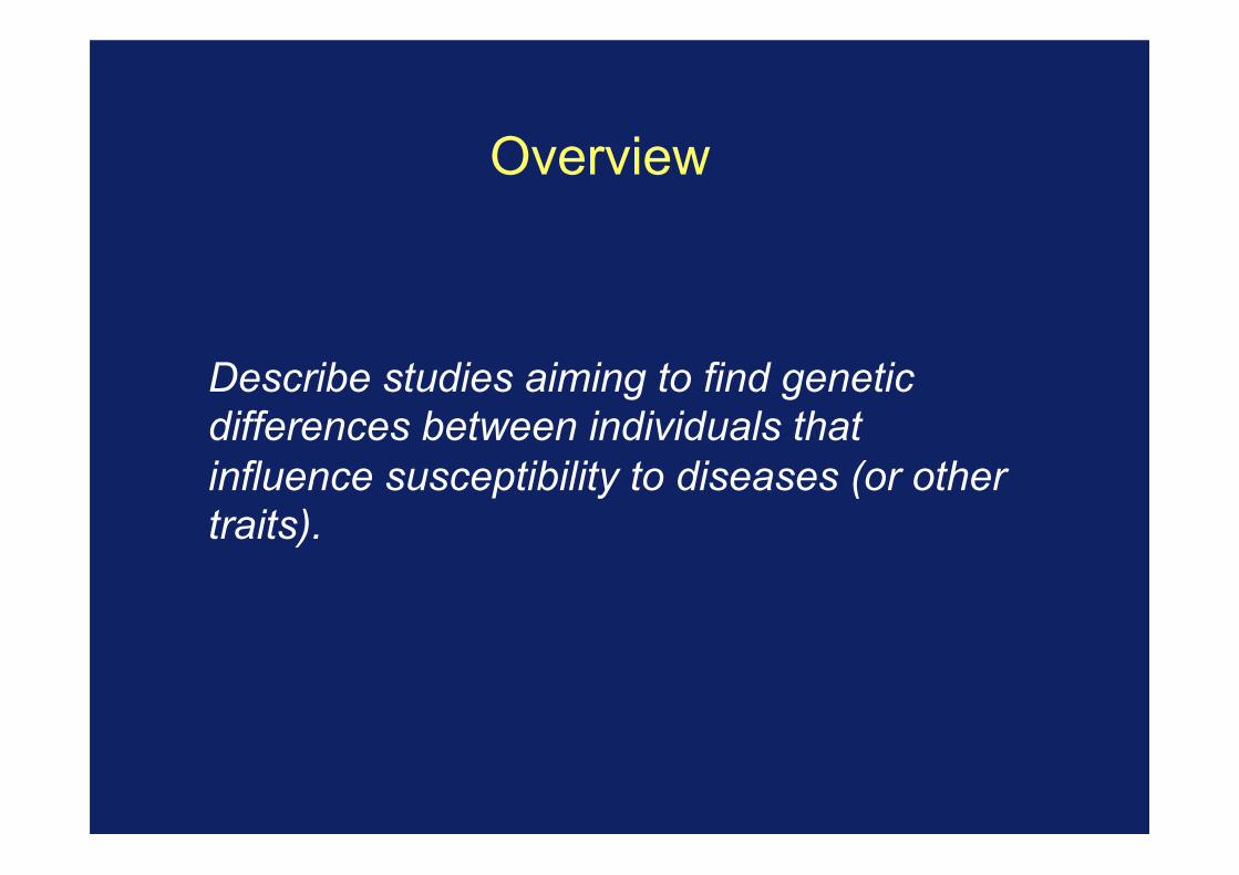
Why find “disease genes”? Genetic factors are particularly interesting because (unlike environmental factors) they are: •  inherited at birth •  essentially unchanging •  (often) easily measurable

This makes inferences about causation particularly simple. e.g. compare: “cyclists tend to be taller” => causation could plausibly work either way “people with genotype AA tend to be taller” => implies causation (all else being equal)

Inheritance = nature’s randomised control trial

Why find “disease genes”? Genetic factors are particularly interesting because (unlike environmental factors) they are: •  inherited at birth •  essentially unchanging •  (often) easily measurable

Reasons to look for disease genes: •  Identify drug targets •  Predict risk of disease •  Personalised medicine (e.g. stratified by likely treatment response) •  Gene therapy? •  etc...

•  ...understand the biology of disease

The circle of genetic causation (a causal mutation)

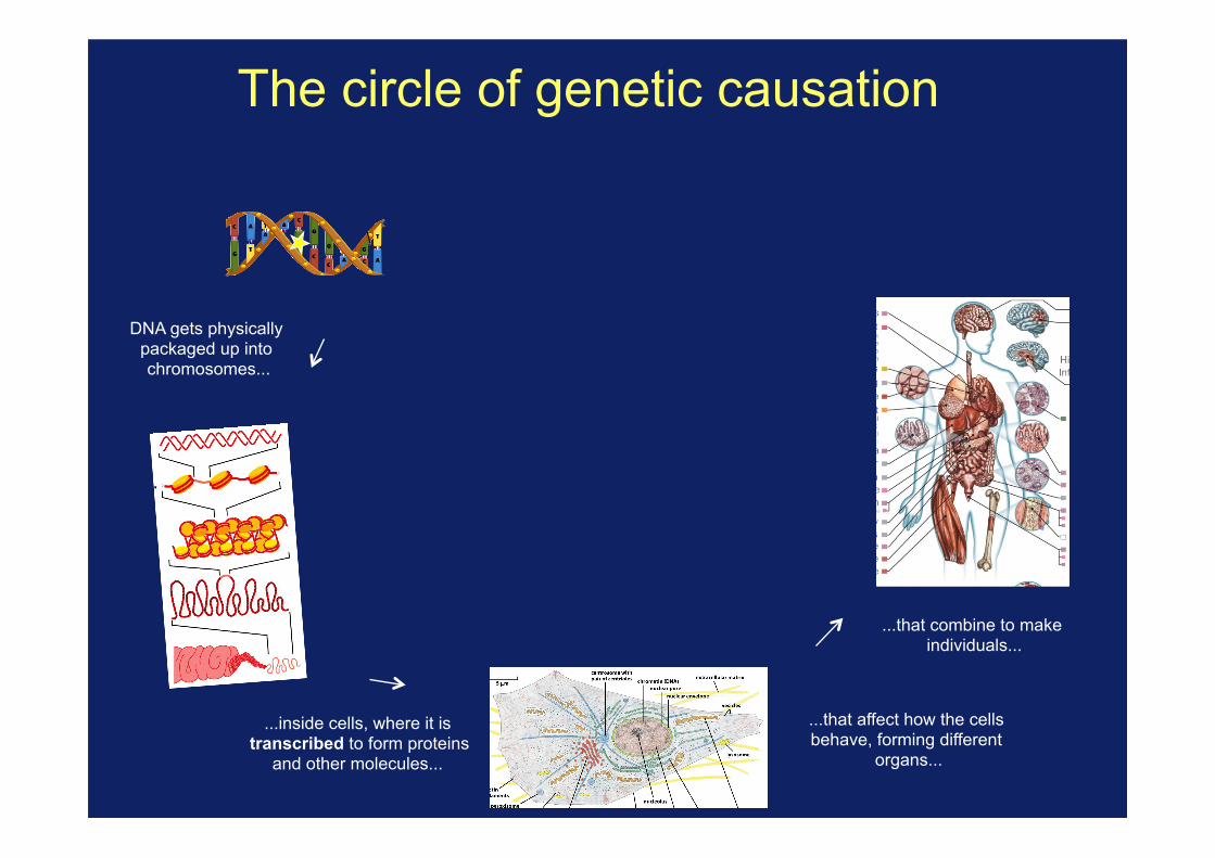
The circle of genetic causation

DNA gets physically packaged up into chromosomes...


...inside cells, where it is transcribed to form proteins

and other molecules...





...that affect how the cells behave, forming different

organs...


...that combine to make individuals...





organs...

...whose success is affected by the traits they have...



The circle of genetic causation ...passing on DNA, with

mutations and recombination, to new

generations...




organs...


...that gets physically packaged up into chromosomes...


The circle of genetic causation ...passing on DNA, with

mutations and recombination, to new

generations...




organs...


...that gets physically packaged up into chromosomes...


All of this can now be

measured

RFLP, microarrays, genome sequencing

Chromatin state marker assays,

ChIP-seq, ...

RNA-seq, spectroscopy, antibody

binding

Biomarker measurements

Clinical phenotype measurements

Summary 1

It is clinically useful and interesting to look for the genetic variants underlying human traits The mapping of genetics to traits is likely to be complex because of the complex processes involved. Now’s an exciting time to be working on this - we now have the technology to attack it at large scale.

Decade Technology #variants Discovery

1800s 0 Pre-molecular genetics (Darwin; Mendel; Galton...)

1900s Handful Discovery of 1st human polymorphism (the ABO blood group)

1950s Structure of DNA published

1970s “Sanger sequencing”

Handful Low-throughout sequencing

1980s RFLPs; PCR;

100s First genetic marker linked to a disease (Cystic Fibrosis) found using a genetic linkage study.

1990s Human Genome Project started. Linkage studies with 1,000s of markers.

2000’s Microarrays 105-106 Human genome assembly completed; first surveys of human genetic variation (International HapMap project); first microarrays; first genome-wide association studies (GWAS).

2010’s high-throughput sequencing

Whole genome

Mapping of all common human variation (1000 Genomes Project); GWAS meta-analyses; direct-to-consumer genotype testing

Today Very large scale ‘biobank’ / population sequencing projects.

Genomics timeline

Finding disease genes in practice

  I’m going to assume we’ve got a trait that we’ve established is heritable

  We want to find genetic variants influencing it. How?

Finding disease genes in practice

Demonstration by Francis Galton that human height is heritable (height of parents predicts height of offspring).

Finding needles in the haystack

The human genome is 3.2 billion base pairs long

We want to find a small number of ‘causal’ genetic mutations in there. How?

Luckily, nature has given us a way to narrow down on specific regions of the genome.

Recombination

Mother Father

Offspring

Genetic recombination breaks up the DNA into segments. You inherit a mosaic of segments of your parents’ DNA.

Recombination = nature’s magnifying glass

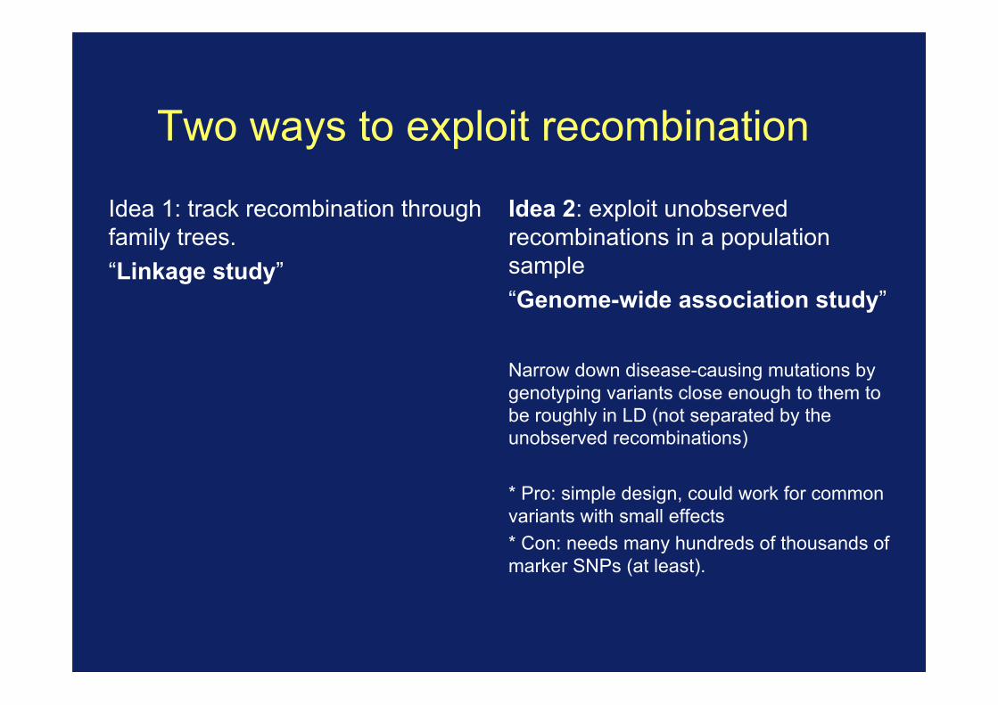
Two ways to exploit recombination

Idea 1: track recombination through family trees. “Linkage study” * Narrow down a disease-causing mutation by assessing where it lies among recombination events observed in one or more families

* Pro: not that many markers needed (100s or 1000s maybe). * Con: not that good resolution, and will only work for rare mutations with strong effects.

Idea 2: exploit unobserved recombinations in a population sample “Genome-wide association study”

ABC abc

abc abc

ABC abc

abc abc

aBC abc

Abc abc

ABC abc

abC abc

abc abc

ABc abc

ABC abc

= Affected

= Unaffected

Linkage Mapping exploits recombination in families

A chromosome

A/a B/b C/c …

Small number of typed markers

Linkage Mapping Linkage Studies in Alzheimer Disease

Multipoint Results forCH 19 Markers D 1 9S 1 3-ATP 1 A3-BCL3 for FAD Families

Age Curve vs. Affecteds Only

LUw0Uco0-J

z

0.-JD

1.

I

/ \ I\ Il

LOCATION (Morgans)

Figure 2 CH19 multipoint analysis in 32 FAD families combining both early- (M K 60 years) and late-onset (M > 60 years) families.The unbroken line ( ) represents the age curve (early and late onset), and the broken line (-- -) represents affected only (early andlate onset).

only those families that fit the criteria outlined byHaines et al. (1988), who suggested selecting onlythose families that had both evidence for 3-genera-tion-affected data and at least three tested affecteds(one of which could be an individual whose genotypeis inferred from the data on his or her spouse andchildren), thereby reducing the number of sporadiccases and phenocopies that might be included in thedata. When only families meeting these selection crite-ria were analyzed, a peak LOD score of 1.75 for theage-adjusted data and of 2.04 for affecteds only was

obtained (when FAD was located between D19S13and ATP1AB).

D. Heterogeneity AnalysisThe results of the A-tests for heterogeneity using

both the two-point and multipoint linkage results forthe CH19 markers alone were not significant for eitherthe age-adjusted or affecteds-only analyses. Similar re-

sults were found when the CH21 markers were used.

When both the CH19 and CH21 multipoint resultswere examined simultaneously, the results of theaffecteds-only analysis were still not significant, butthe age-adjusted analyses were nearing significance(P = .09) with an estimate of the proportion ofCH19-linked families being .65. Combining our two-point data for D21S1 /S11 with the published data ofSt. George Hyslop et al. (1990) also failed to reachstatistical significance in the A-test (P = .27).When the PDS test applied to the data in order to

detect heterogeneity between the two groups used <60years as the cutoff for the early-onset families, theresults neared significance (P = .06). Similar resultswere found when the test applied to our data used <65and <70 years as the cutoff for early-onset families.Combining these data with the data of St. George Hys-lop et al. (1990) showed significant results (P < .05).Significant results (P < .01) were also found for thecombined data sets when cutoffs of 65 and 70 yearswere used for the grouping of early- versus late-onsetfamilies.

1045Typical result if successful – a strong signal (good) but not well localised within a chromosome.

chromosome 19

This initial discovery – based on 32 extended families - led to finding of APOE variants affecting risk of Alzheimers.

Pericak-Vance et al, Am. J. Hum. Gen (1991)

Lots of linkage studies were published in the 1980’s – early 90’s

Successes and Failures circa 2000

Linkage Mapping was successful in identifying the genetic basis of many human diseases in which the disease penetrance resembles a simple Mendelian model e.g. Huntington’s disease (HD 1993), Cystic Fibrosis, some forms of breast cancer (BRCA1 1993), Alzheimers (APOE 1991)…

But

“the literature is now replete with linkage screens for an array of common ‘complex’ disorders such as schizophrenia, manic depression, autism, asthma, type I and type II diabetes, Multiple Sclerosis, Lupus. Although many of these studies have reported significant linkage findings,

none has lead to convincing replication” – Risch (2000)

Relative risk Relative risk measures the chance of getting disease if exposed to the risk genotype, versus the chance if not exposed:

Relative risk = P( disease | carry risk allele )

P( disease | don’t carry the risk allele )

For a ‘Mendelian’-like trait e.g. driven by a single highly penetrant mutation:

=> RR = 4 or more You are many times more likely to get disease if you carry

the risk allele. Example: RR ~ 20 for the Alzheimers variant APOE e4.

Relative risk

Relative risk = P( disease | carry risk allele )

P( disease | don’t carry the risk allele )

But most common diseases are now thought to be influenced by multiple common variants with small effects

e.g. RR < 1.5 or smaller.

Relative risk measures the chance of getting disease if exposed to the risk genotype, versus the chance if not exposed:

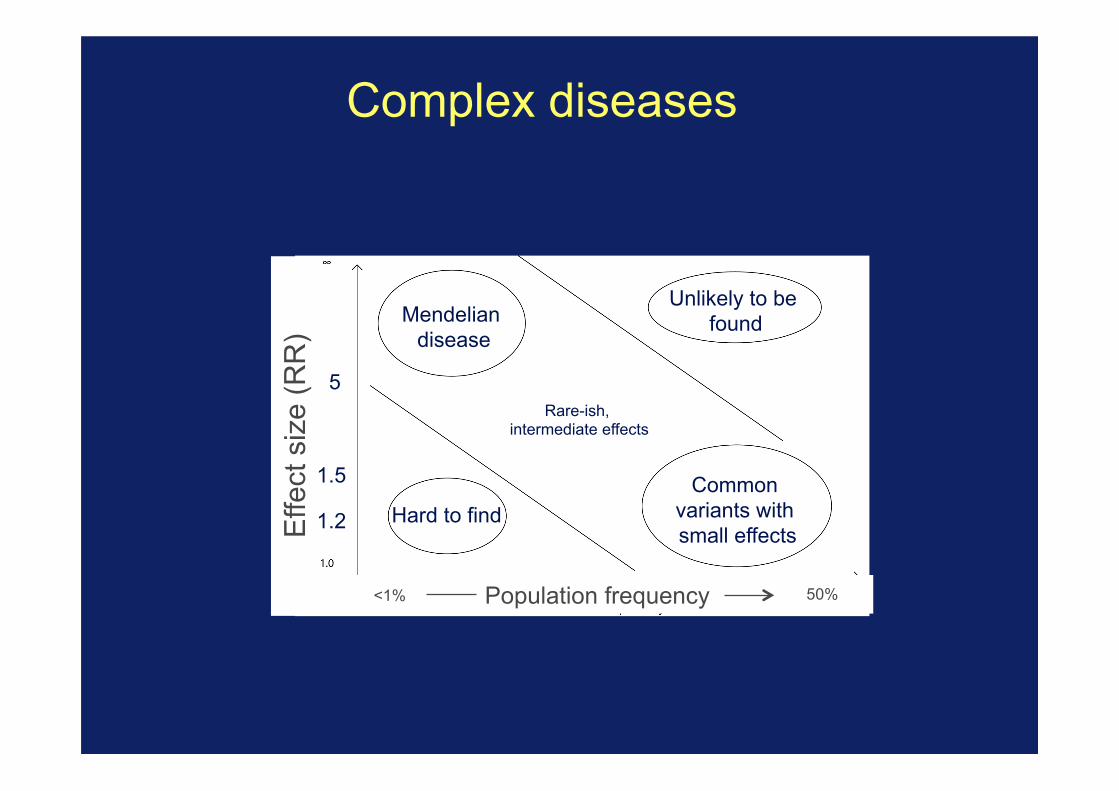
Complex diseases

Effe

ct s

ize

(RR

)

Population frequency <1% 50%

5

1.2

1.5 Common variants with small effects

Mendelian disease

Unlikely to be found

Hard to find

Rare-ish, intermediate effects

Complex diseases

Effe

ct s

ize

(RR

)

Population frequency <1% 50%

5

1.2

1.5 Common variants with small effects

Mendelian disease

Unlikely to be found

Hard to find

Rare-ish, intermediate effects

Where linkage studies are likely to work

Where most complex disease effects are

Two ways to exploit recombination

Idea 1: track recombination through family trees. “Linkage study”

Idea 2: exploit unobserved recombinations in a population sample “Genome-wide association study” Narrow down disease-causing mutations by genotyping variants close enough to them to be roughly in LD (not separated by the unobserved recombinations) * Pro: simple design, could work for common variants with small effects * Con: needs many hundreds of thousands of marker SNPs (at least).

Association testing

Mother Father

Offspring

Genetic recombination breaks up the DNA into segments. You inherit a mosaic of segments of your parents’ DNA.

Recombination = nature’s magnifying glass

Association testing

Time

Mutation arises

Gets passed on through many generations

Still carries a little bit of its original haplotype, broken up by recombination

=> Causal mutation will be still be correlated with those near it. If we could type enough markers, could access it

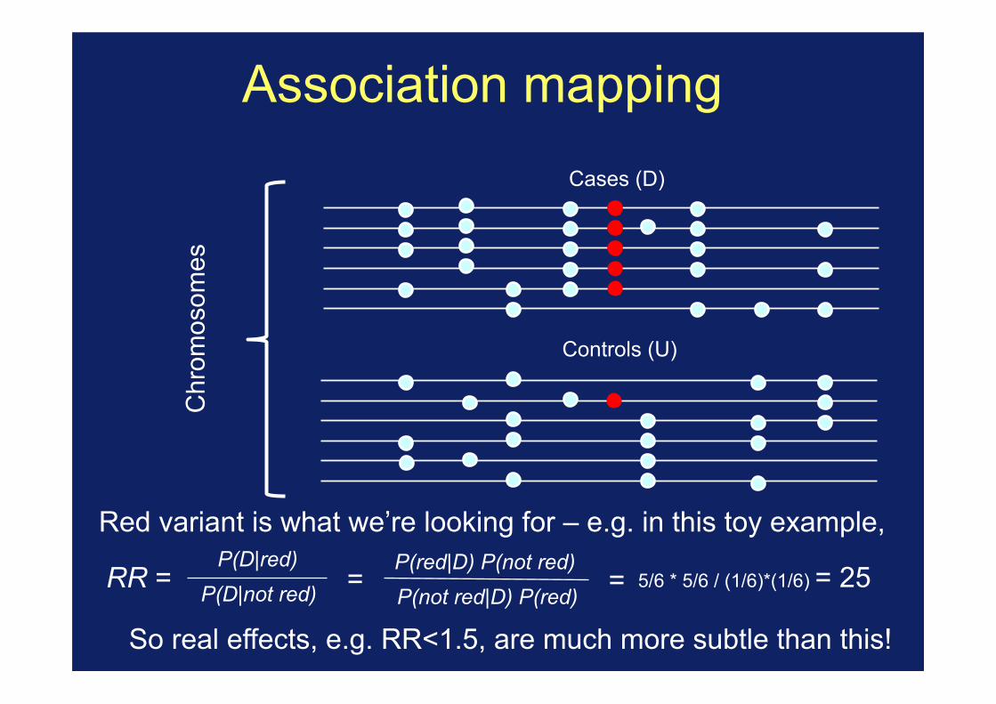
Cases (D)

Controls (U)

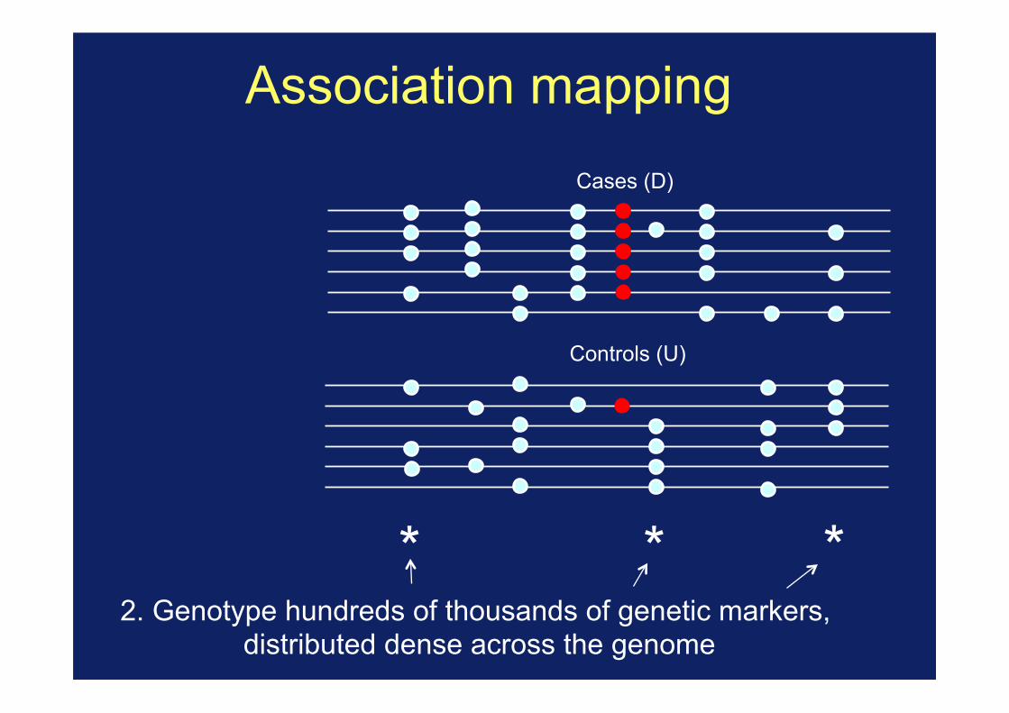
Association mapping

1. Collect a set of unrelated affected individuals (cases) and unaffected individuals (controls).

Chr

omos

omes

Cases (D)

Controls (U)

Association mapping

Red variant is what we’re looking for – e.g. in this toy example,

Chr

omos

omes

P(D|not red) P(D|red)

P(not red|D) P(red) P(red|D) P(not red)

= RR = = 5/6 * 5/6 / (1/6)*(1/6) = 25

So real effects, e.g. RR<1.5, are much more subtle than this!

Cases (D)

Controls (U)

* * * 2. Genotype hundreds of thousands of genetic markers,

distributed dense across the genome

Association mapping

Cases (D)

Controls (U)

* * *

Association mapping

3. Rely on correlations (or LD) between typed markers and the causal mutations

Association mapping

e.g in our toy example

Not white white

cases 5 1 controls 2 4

=> Estimate RR=10 at this marker SNP.

Perform statistical test to test for evidence of difference in allele frequencies between cases and controls. (e.g. chi-squared test). In this toy example P=0.24 so not enough data even for this strong effect.

Frequency

1/6 2/3

P-value < (a stringent threshhold) => success!

(Aside - association studies – TDT)

A a

a a

A a

A A

Collect (lots) of trios of individuals Condition on phenotype of offspring (case) High risk alleles should be over transmitted Internal control formed by untransmitted alleles

Difference between linkage and association Linkage studies   - Collect set of families with individuals carrying disease or

phenotype   - Look for co-segregation of small number of markers with

disease status.   - Relies on inheritance of large segments of DNA

seperated by a few genetic recombinations

Association Studies - Collect unrelated individuals and look at allele frequency differences between cases and controls (or cases and parents for TDT) - Requires genotyping hundreds of thousands of markers. - Relies on the many unobserved recombinations leaving correlations between nearby genetic variants along chromosomes within the population

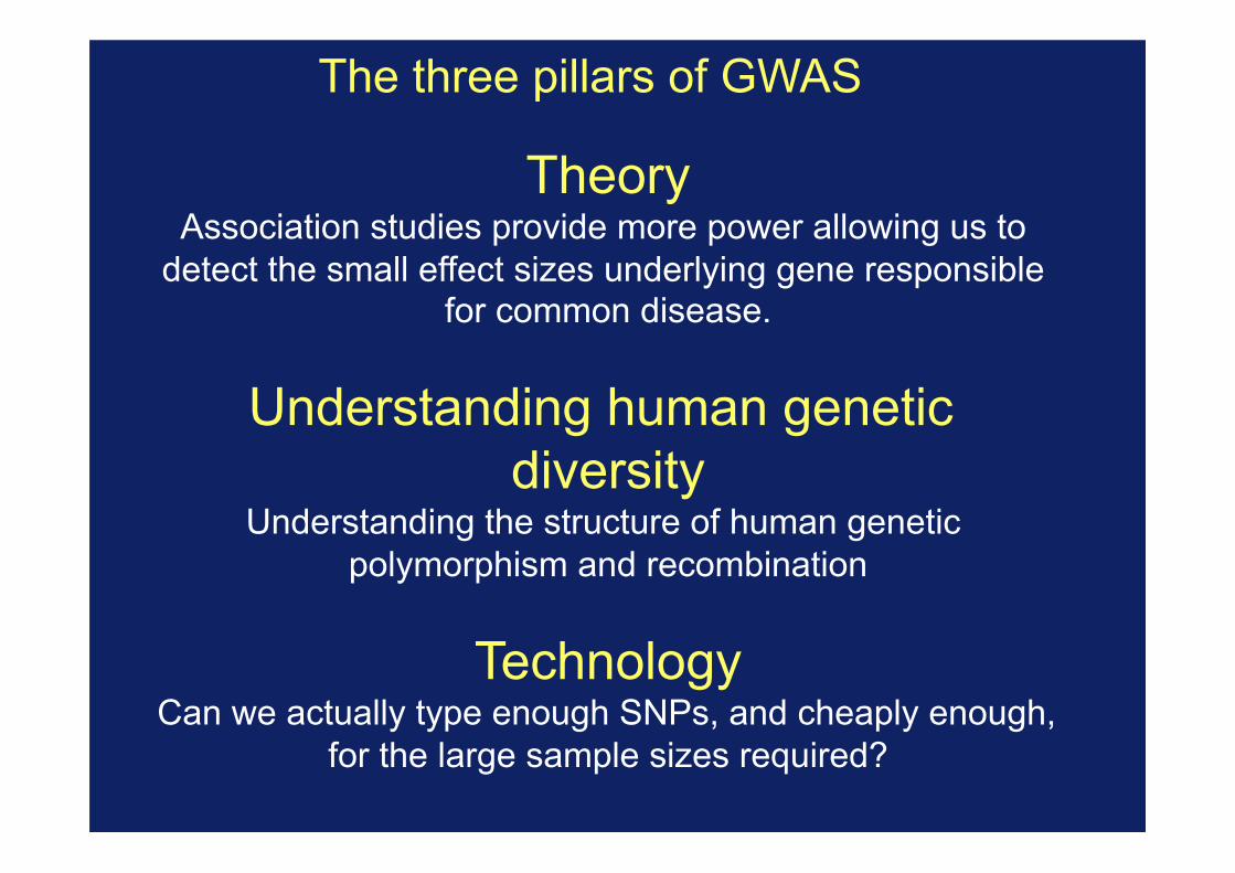
Theory Association studies provide more power allowing us to

detect the small effect sizes underlying gene responsible for common disease.

Understanding human genetic diversity

Understanding the structure of human genetic polymorphism and recombination

Technology Can we actually type enough SNPs, and cheaply enough,

for the large sample sizes required?

The three pillars of GWAS

Tagging genetic diversity

How many markers are actually required to tag the diversity?

- To understand this, must first understand patterns of diversity in natural populations

- Identify catalogue of variants to type

Can we design experiments to analyse such large numbers of SNPs?

Decade Technology #variants Discovery

1800s 0 Pre-molecular genetics (Darwin; Mendel; Galton...)

1900s Handful Discovery of 1st human polymorphism (the ABO blood group)

1950s Structure of DNA published

1970s “Sanger sequencing”

Handful Low-throughout sequencing

1980s RFLPs; PCR;

100s First genetic marker linked to a disease (Cystic Fibrosis) found using a genetic linkage study.

1990s Human Genome Project started. Linkage studies with 1,000s of markers.

2000’s Microarrays 105-106 Human genome assembly completed; first surveys of human genetic variation (International HapMap project); first microarrays; first genome-wide association studies (GWAS).

2010’s high-throughput sequencing

Whole genome

Map of all common human variation (1000 Genomes Project); GWAS meta-analyses; direct-to-consumer genotype testing

Today Very large scale ‘biobank’ / population sequencing projects.

Genomics timeline

© 2005 Nature Publishing Group

A haplotype map of the human genomeThe International HapMap Consortium*

Inherited genetic variation has a critical but as yet largely uncharacterized role in human disease. Here we report apublic database of common variation in the human genome: more than one million single nucleotide polymorphisms(SNPs) for which accurate and complete genotypes have been obtained in 269 DNA samples from four populations,including ten 500-kilobase regions in which essentially all information about common DNA variation has been extracted.These data document the generality of recombination hotspots, a block-like structure of linkage disequilibrium and lowhaplotype diversity, leading to substantial correlations of SNPs with many of their neighbours. We show how theHapMap resource can guide the design and analysis of genetic association studies, shed light on structural variation andrecombination, and identify loci that may have been subject to natural selection during human evolution.

Despite the ever-accelerating pace of biomedical research, the rootcauses of common human diseases remain largely unknown, pre-ventativemeasures are generally inadequate, and available treatmentsare seldom curative. Family history is one of the strongest risk factorsfor nearly all diseases—including cardiovascular disease, cancer,diabetes, autoimmunity, psychiatric illnesses and many others—providing the tantalizing but elusive clue that inherited geneticvariation has an important role in the pathogenesis of disease.Identifying the causal genes and variants would represent an impor-tant step in the path towards improved prevention, diagnosis andtreatment of disease.More than a thousand genes for rare, highly heritable ‘mendelian’

disorders have been identified, in which variation in a single gene isboth necessary and sufficient to cause disease. Common disorders, incontrast, have proven much more challenging to study, as theyare thought to be due to the combined effect of many differentsusceptibility DNA variants interacting with environmental factors.Studies of common diseases have fallen into two broad categories:

family-based linkage studies across the entire genome, and popu-lation-based association studies of individual candidate genes.Although there have been notable successes, progress has been slowdue to the inherent limitations of the methods; linkage analysis haslow power except when a single locus explains a substantial fractionof disease, and association studies of one or a few candidate genesexamine only a small fraction of the ‘universe’ of sequence variationin each patient.A comprehensive search for genetic influences on disease would

involve examining all genetic differences in a large number of affectedindividuals and controls. It may eventually become possible toaccomplish this by complete genome resequencing. In the meantime,it is increasingly practical to systematically test common geneticvariants for their role in disease; such variants explain much of thegenetic diversity in our species, a consequence of the historicallysmall size and shared ancestry of the human population.Recent experience bears out the hypothesis that common variants

have an important role in disease, with a partial list of validatedexamples including HLA (autoimmunity and infection)1, APOE4(Alzheimer’s disease, lipids)2, Factor VLeiden (deep vein thrombosis)3,PPARG (encoding PPARg; type 2 diabetes)4,5, KCNJ11 (type 2

diabetes)6, PTPN22 (rheumatoid arthritis and type 1 diabetes)7,8,insulin (type 1 diabetes)9,CTLA4 (autoimmune thyroid disease, type1 diabetes)10, NOD2 (inflammatory bowel disease)11,12, complementfactor H (age-related macular degeneration)13–15 and RET (Hirsch-sprung disease)16,17, among many others.Systematic studies of common genetic variants are facilitated by

the fact that individuals who carry a particular SNP allele at one siteoften predictably carry specific alleles at other nearby variant sites.This correlation is known as linkage disequilibrium (LD); a particu-lar combination of alleles along a chromosome is termed a haplotype.LD exists because of the shared ancestry of contemporary chromo-

somes.When a new causal variant arises throughmutation—whethera single nucleotide change, insertion/deletion, or structural altera-tion—it is initially tethered to a unique chromosome on which itoccurred, marked by a distinct combination of genetic variants.Recombination and mutation subsequently act to erode this associ-ation, but do so slowly (each occurring at an average rate of about1028 per base pair (bp) per generation) as compared to the numberof generations (typically 104 to 105) since the mutational event.The correlations between causal mutations and the haplotypes on

which they arose have long served as a tool for human geneticresearch: first finding association to a haplotype, and then sub-sequently identifying the causal mutation(s) that it carries. This waspioneered in studies of the HLA region, extended to identify causalgenes for mendelian diseases (for example, cystic fibrosis18 anddiastrophic dysplasia19), and most recently for complex disorderssuch as age-related macular degeneration13–15.Early information documented the existence of LD in the human

genome20,21; however, these studies were limited (for technicalreasons) to a small number of regions with incomplete data, andgeneral patterns were challenging to discern. With the sequencing ofthe human genome and development of high-throughput genomicmethods, it became clear that the human genome generallydisplays more LD22 than under simple population genetic models23,and that LD is more varied across regions, and more segmentallystructured24–30, than had previously been supposed. These obser-vations indicated that LD-based methods would generally havegreat value (because nearby SNPs were typically correlated withmany of their neighbours), and also that LD relationships would

ARTICLES

*Lists of participants and affiliations appear at the end of the paper.

Vol 437|27 October 2005|doi:10.1038/nature04226

1299

International HapMap Project (circa 2000)

Understanding human genetic diversity

ARTICLE OPENdoi:10.1038/nature15393

A global reference for humangenetic variationThe 1000 Genomes Project Consortium*

The 1000 Genomes Project set out to provide a comprehensive description of common human genetic variation byapplying whole-genome sequencing to a diverse set of individuals from multiple populations. Here we reportcompletion of the project, having reconstructed the genomes of 2,504 individuals from 26 populations using a combina-tion of low-coverage whole-genome sequencing, deep exome sequencing, and dense microarray genotyping. Wecharacterized a broad spectrum of genetic variation, in total over 88 million variants (84.7 million single nucleotidepolymorphisms (SNPs), 3.6 million short insertions/deletions (indels), and 60,000 structural variants), all phasedonto high-quality haplotypes. This resource includes .99% of SNP variants with a frequency of .1% for a variety ofancestries. We describe the distribution of genetic variation across the global sample, and discuss the implications forcommon disease studies.

The 1000 Genomes Project has already elucidated the properties anddistribution of common and rare variation, provided insights into theprocesses that shape genetic diversity, and advanced understanding ofdisease biology1,2. This resource provides a benchmark for surveys ofhuman genetic variation and constitutes a key component for humangenetic studies, by enabling array design3,4, genotype imputation5,cataloguing of variants in regions of interest, and filtering of likelyneutral variants6,7.

In this final phase, individuals were sampled from 26 populationsin Africa (AFR), East Asia (EAS), Europe (EUR), South Asia (SAS),and the Americas (AMR) (Fig. 1a; see Supplementary Table 1 forpopulation descriptions and abbreviations). All individuals weresequenced using both whole-genome sequencing (mean depth 5 7.43)and targeted exome sequencing (mean depth 5 65.73). In addition,individuals and available first-degree relatives (generally, adult off-spring) were genotyped using high-density SNP microarrays. This pro-vided a cost-effective means to discover genetic variants and estimateindividual genotypes and haplotypes1,2.

Data set overviewIn contrast to earlier phases of the project, we expanded analysisbeyond bi-allelic events to include multi-allelic SNPs, indels, and adiverse set of structural variants (SVs). An overview of the samplecollection, data generation, data processing, and analysis is given inExtended Data Fig. 1. Variant discovery used an ensemble of 24sequence analysis tools (Supplementary Table 2), and machine-learn-ing classifiers to separate high-quality variants from potential falsepositives, balancing sensitivity and specificity. Construction of hap-lotypes started with estimation of long-range phased haplotypes usingarray genotypes for project participants and, where available, theirfirst degree relatives; continued with the addition of high confidencebi-allelic variants that were analysed jointly to improve these haplo-types; and concluded with the placement of multi-allelic and struc-tural variants onto the haplotype scaffold one at a time (Box 1).Overall, we discovered, genotyped, and phased 88 million variant sites(Supplementary Table 3). The project has now contributed orvalidated 80 million of the 100 million variants in the public dbSNPcatalogue (version 141 includes 40 million SNPs and indels newly

contributed by this analysis). These novel variants especiallyenhance our catalogue of genetic variation within South Asian (whichaccount for 24% of novel variants) and African populations (28% ofnovel variants).

To control the false discovery rate (FDR) of SNPs and indels at,5%, a variant quality score threshold was defined using high depth(.303) PCR-free sequence data generated for one individual perpopulation. For structural variants, additional orthogonal methodswere used for confirmation, including microarrays and long-readsequencing, resulting in FDR , 5% for deletions, duplications,multi-allelic copy-number variants, Alu and L1 insertions, and,20% for inversions, SVA (SINE/VNTR/Alu) composite retrotran-sposon insertions and NUMTs8 (nuclear mitochondrial DNA var-iants). To evaluate variant discovery power and genotypingaccuracy, we also generated deep Complete Genomics data (meandepth 5 473) for 427 individuals (129 mother–father–child trios,12 parent–child duos, and 16 unrelateds). We estimate the power todetect SNPs and indels to be .95% and .80%, respectively, forvariants with sample frequency of at least 0.5%, rising to .99% and.85% for frequencies .1% (Extended Data Fig. 2). At lower frequen-cies, comparison with .60,000 European haplotypes from theHaplotype Reference Consortium9 suggests 75% power to detectSNPs with frequency of 0.1%. Furthermore, we estimate heterozygousgenotype accuracy at 99.4% for SNPs and 99.0% for indels(Supplementary Table 4), a threefold reduction in error rates com-pared to our previous release2, resulting from the larger sample size,improvements in sequence data accuracy, and genotype calling andphasing algorithms.

A typical genomeWe find that a typical genome differs from the reference humangenome at 4.1 million to 5.0 million sites (Fig. 1b and Table 1).Although .99.9% of variants consist of SNPs and short indels,structural variants affect more bases: the typical genome containsan estimated 2,100 to 2,500 structural variants (,1,000 large dele-tions, ,160 copy-number variants, ,915 Alu insertions, ,128 L1insertions, ,51 SVA insertions, ,4 NUMTs, and ,10 inversions),affecting ,20 million bases of sequence.

6 8 | N A T U R E | V O L 5 2 6 | 1 O C T O B E R 2 0 1 5

*Lists of participants and their affiliations appear in the online version of the paper.

G2015 Macmillan Publishers Limited. All rights reserved

1000 Genomes Project (circa 2010)

Discovery of over 5M SNPs across the gneome

Discovery of over 80M SNPs and indels across

the gneome

More correlation between SNPs (LD) than had been thought

Physical distance along chromosome

Cor

rela

tion

Real data

Previous prediction

Reich et al Nature 2001

Why? - recombination hotspots

Count the number of recombination in (lots) of sperm in the MHC region of chromosome 6

Jeffreys et al 1998

Hotspots are a genome wide feature

More than 80% of recombination in less than 10% of the genome

© 2005 Nature Publishing Group

varies by chromosome; when plotted against average recombinationrate on each chromosome (estimated from pedigree-based geneticmaps) these differences largely disappear (Supplementary Fig. 6).Similarly, the distribution of haplotype length across chromosomesis less variable when measured in genetic rather than physicaldistance. For example, the median length of haplotypes is 54.4 kbon chromosome 1 compared to 34.8 kb on chromosome 21. Whenmeasured in genetic distance, however, haplotype length is muchmore similar: 0.104 cM on chromosome 1 compared to 0.111 cM onchromosome 21 (Supplementary Fig. 9).The exception is again the X chromosome, which has more

extensive haplotype structure after accounting for recombinationrate (median haplotype length ¼ 0.135 cM). Multiple factors could

explain different patterns on the X chromosome: lower SNP density,smaller sample size, restriction of recombination to females andlower effective population size.

A view of LD focused on the putative causal SNPAlthough genealogy and recombination provide insight into whynearby SNPs are often correlated, it is the redundancies among SNPsthat are of central importance for the design and analysis ofassociation studies. A truly comprehensive genetic associationstudy must consider all putative causal alleles and test each for itspotential role in disease. If a causal variant is not directly tested in thedisease sample, its effect can nonetheless be indirectly tested if it iscorrelated with a SNP or haplotype that has been directly tested.

Figure 8 | Comparison of linkage disequilibrium and recombination for twoENCODE regions. For each region (ENr131.2q37.1 and ENm014.7q31.33),D 0 plots for the YRI, CEU and CHBþJPTanalysis panels are shown: white,D 0 , 1 and LOD , 2; blue, D 0 ¼ 1 and LOD , 2; pink, D 0 , 1 andLOD $ 2; red,D 0 ¼ 1 and LOD $ 2. Below each of these plots is shown the

intervals where distinct obligate recombination events must have occurred(blue and green indicate adjacent intervals). Stacked intervals representregions where there aremultiple recombination events in the sample history.The bottom plot shows estimated recombination rates, with hotspots shownas red triangles46.

NATURE|Vol 437|27 October 2005 ARTICLES

1307

Recombination gives LD a block-like structure

International HapMap Project

HapMap project Consortium of a large number of scientist to conduct a

study to catalogue and describe human genetic diversity

Estimate that 200,000 to 500,000 SNPs require to tag genome (at least in European and Asian populations).

Competition drove technology improvements

Affymetrix 100K   Affymetrix 500K   Affymetrix 6.0 (~1M SNPs)   …   Illumina 650Y   Illumina 1M   Illumina 2.5M   Illumina 5M   …   Which one to buy?

Coverage

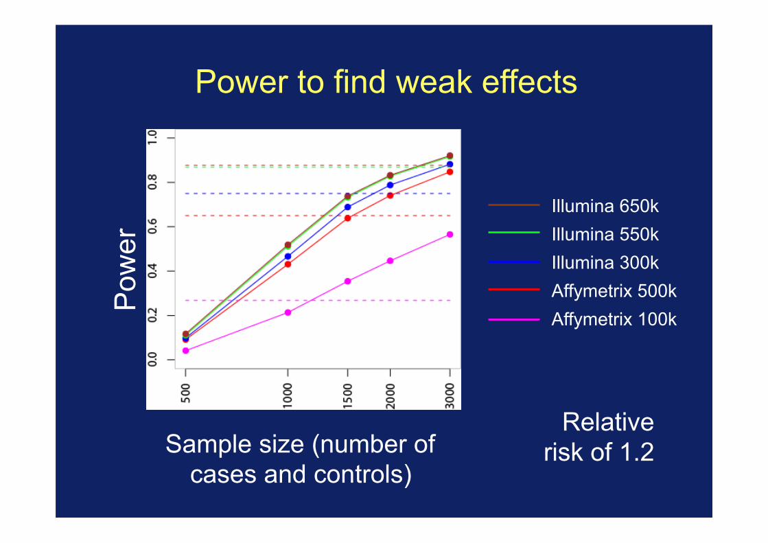
Power to find weak effects

Illumina 650k Illumina 550k Illumina 300k Affymetrix 500k Affymetrix 100k

Pow

er

Sample size (number of cases and controls)

Relative risk of 1.2

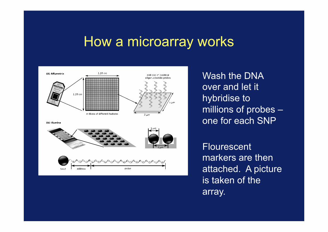
How a microarray works

Wash the DNA over and let it hybridise to millions of probes – one for each SNP

Flourescent markers are then attached. A picture is taken of the array.

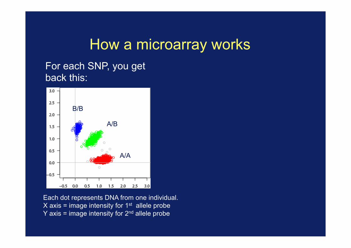
How a microarray works For each SNP, you get back this:

Each dot represents DNA from one individual. X axis = image intensity for 1st allele probe Y axis = image intensity for 2nd allele probe

B/B

A/B

A/A

How a microarray works For each SNP, you get back this:

Each dot represents DNA from one individual. X axis = image intensity for 1st allele probe Y axis = image intensity for 2nd allele probe

B/B

A/B

A/A

Or this if you’re less lucky:

B/B? A/B?

A/A?

?

?

This is one of several things that can go wrong, and needs to be dealt with. More examples next week.

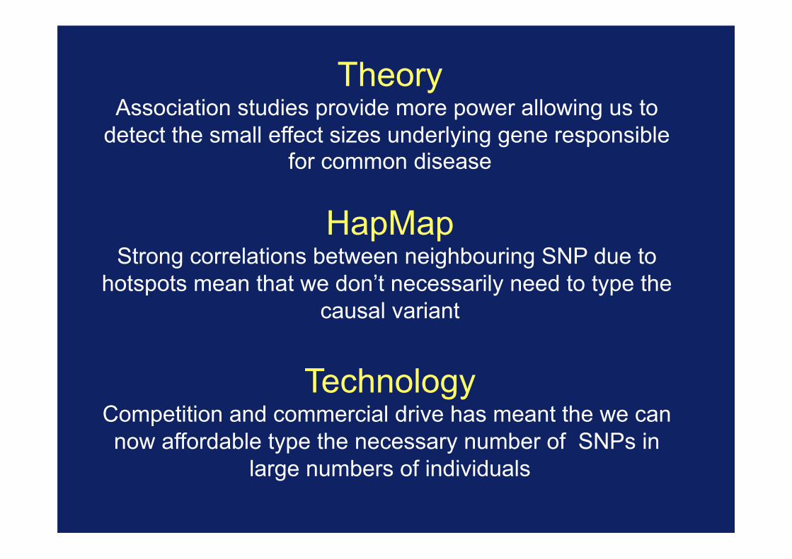
Theory Association studies provide more power allowing us to

detect the small effect sizes underlying gene responsible for common disease

HapMap Strong correlations between neighbouring SNP due to

hotspots mean that we don’t necessarily need to type the causal variant

Technology

Competition and commercial drive has meant the we can now affordable type the necessary number of SNPs in

large numbers of individuals

GWAS recipe

  1. Collect large numbers of case individuals (1000s)   2. Collect large numbers of controls (perhaps

randomly from the population).   (3. Get consent)   4. Extract DNA   5. Genotype individuals at lots of markers   6. Throw away data – poor quality samples, poorly

genotyped SNPs...   7. At each SNP do a test for allele frequency

difference between cases and controls (chi-squared, logistic regression)

  8. Look for small p-values (how small)?

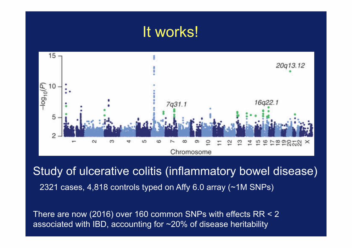
It works!

Study of ulcerative colitis (inflammatory bowel disease) 2321 cases, 4,818 controls typed on Affy 6.0 array (~1M SNPs)

There are now (2016) over 160 common SNPs with effects RR < 2 associated with IBD, accounting for ~20% of disease heritability

It works!

Study of multiple sclerosis (2011) 9772 cases, 17,376 controls from across Europe

www.well.ox.ac.uk/wtccc2/ms

https://www.ebi.ac.uk/gwas/diagram

Over 20,000 identified signals of association

Summary 2

It is clinically useful and interesting to look for the genetic variants underlying human traits Genetic factors underlying common traits are often quite common and have small effects Now’s an exciting time to be working on this - we now have the technology to attack it at large scale. Next week: look in detail at some real studies

Homework

Visit http://www.well.ox.ac.uk/wtccc2/ms

Play around with the site and make sure you understand the different things that are shown.

Documents

Multifactorial traits and complex genetics - well.ox.ac.ukgav/resources/Genome-wide association studies... · Multifactorial traits and complex genetics Genome-wide association studies