Embed Size (px)
Citation preview

Multifield Visualization Using Local Statistical Complexity
Heike Janicke, Alexander Wiebel, Gerik Scheuermann, Member, IEEE CS, and Wolfgang Kollmann
Abstract— Modern unsteady (multi-)field visualizations require an effective reduction of the data to be displayed. From a hugeamount of information the most informative parts have to be extracted. Instead of the fuzzy application dependent notion of feature, anew approach based on information theoretic concepts is introduced in this paper to detect important regions. This is accomplishedby extending the concept of local statistical complexity from finite state cellular automata to discretized (multi-)fields. Thus, informativeparts of the data can be highlighted in an application-independent, purely mathematical sense. The new measure can be applied tounsteady multifields on regular grids in any application domain. The ability to detect and visualize important parts is demonstratedusing diffusion, flow, and weather simulations.
Index Terms—Local statistical complexity, multifield visualization, time-dependent, coherent structures, feature detection, informationtheory, flow visualization.
1 INTRODUCTION
One of the strengths of scientific visualization is the fact that it cancommunicate large amounts of information. However, images can be-come too crowded and cluttered to see the important facts, too. High-lighting the most informative regions is a powerful method to reducethe amount of information displayed and guide the observers attention.
The crucial step is the extraction of these regions, often called fea-tures. At present, there exists no general definition of a feature, exceptfor being a structure or region of relevance. Depending on the ap-plication, e.g., computational fluid dynamics (CFD), electromagneticfield simulations, weather models or simulations of biological systems,completely different structures are of interest. In general, features aredetected by searching regions that fulfill certain criteria, e.g., exhibita certain value or pattern [29]. As these criteria have to be specifiedin advance, further problems arise. In the case of vortex detection, forexample, no general definition exists. Vortices, however, are not of in-terest because they exhibit some kind of swirling structure, but as theyhave great impact on the behavior of the flow. This property is truefor all features - they are of special importance to the system. More-over, inside these structures it is hard to predict the system’s behavior.Starting from this point, a feature can be characterized as a region thatrequires a lot of information about the past to predict its own dynam-ics. Utilizing information theory, an objective and universal definitionof a feature can be given.
Shalizi et al. [36] proposed a local criterion, called local statis-tical complexity, to measure complexity in cellular automata (CA).Therewith features are identified with regions of high local statisticalcomplexity. As stated in [28, 39], CA can be used to model partial dif-ferential equations (PDEs), and vice versa. The combination of thesetwo approaches results in a general feature extraction method appli-cable to any kind of system that can be described by PDEs, whichcomprise the majority of computational science and engineering sim-ulations. Besides being a generally applicable measure, two additionaladvantages lie in the nature of statistical complexity that many otherfeature detection methods do not have: Firstly, the method is based ontime-dependent analysis, and therefore, can easily cope with unsteady
• Heike Janicke, Alexander Wiebel, and Gerik Scheuermann are with the
Image and Signal Processing Group, Department of Computer Science,
University of Leipzig, Germany.
E-mail: {jaenicke, wiebel, scheuermann}@informatik.uni-leipzig.de.
• Wolfgang Kollmann is with the Department of Mechanical and
Aeronautical Engineering, University of California, Davis. E-mail:
Manuscript received 31 March 2007; accepted 1 August 2007; posted online 2
November 2007.
For information on obtaining reprints of this article, please send e-mail to:
datasets. And secondly, from an information theoretic point of viewmultifield analysis is required and directly realized if the system is in-fluenced by several independent variables. In either case, the resultof the analysis is a single time-dependent scalar field, defining impor-tance in the dataset.
2 RELATED WORK
Most datasets obtained by measurements or numerical simulations arecombinations of different quantities. Though many methods in thefield of scientific visualization focus on the analysis of a single field,there are several approaches treating multiple fields at a time. In gen-eral, two different approaches can be distinguished. Either severalfields are visualized in combination, or relations between the differ-ent fields are displayed. Examples of the first approach are mostlycombinations of different techniques, e.g., color coding, glyphs and/orpartially transparent maps as used by Bair et al. [3] or Kirby et al. [22]in 2D, and modified volume rendering in 3D (Andreassen [1], Riley[30]). The analysis of correlation between different fields belongs tothe second category and was researched amongst others by Kniss et al.[23] and Sauber et al. [33]. A summary of different techniques can befound in [40].
Many multifield methods suffer from cluttering if the number offields gets too large. An efficient way to reduce cluttering is to con-centrate on relevant structures or regions, so called features. High-lighting important regions does not only reduce the amount of data tobe displayed significantly without losing important information, butalso focuses the observers attention. Consequently, features have tobe extracted first. As there is no general feature definition so far, thereexists no universal method to detect them. In the literature three differ-ent approaches can be distinguished: image processing (e.g. Ebling etal. [9], Heiberg et al. [17]), topological analysis (e.g. Scheuermann etal. [34]) and physical characteristics (e.g. Garth et al. [11], Roth [32]).A detailed description for the field of flow visualization can be foundin [29].
As long as structures are relatively simple, it is possible to definefeatures. But as soon as the systems become more complex, such asanthills, human brains or chemical reactions, the definition of what isrelevant gets more difficult. A first step is to measure the system’scomplexity. A large variety of measures are available fulfilling thistask, e.g., [5, 7, 12, 24, 37]. Common measures originating from theanalysis of strings of data are Shannon entropy [37] and algorithmicinformation [2]. Shannon entropy is a measure of the uncertainty as-sociated with a random variable, whereas the algorithmic informationis roughly speaking the length of the shortest program capable of gen-erating a certain string. Both measures have in common that they aremeasures of randomness. In complex systems however, randomnessis commonly not considered to be complex. Likewise, Hogg and Hu-berman [19] state that complexity is small for completely ordered andcompletely disordered patterns and reaches a maximum inbetween. A

spac
e
timet-3
t-2
t-1
t0
t1
Fig. 1. Illustration of the past (blue) and future light-cone (red) of a sin-gle position (black cell). Influences propagate at speed c = 1, i.e., onlyimmediately adjacent neighbors affect a cell. The cones are restrictedto past-depth 3 and future-depth 2.
different approach was taken by Grassberger [12], who defined com-plexity as the minimal information that would have to be stored foroptimal predictions. Based on this idea, statistical complexity [7] wasintroduced identifying the complexity of a system with the amount ofinformation needed to specify its causal states, i.e., its classes of iden-tical behavior. In order to analyse random fields, a point-by-point ver-sion was formulated by Shalizi [35] called local statistical complexity.
3 LOCAL STATISTICAL COMPLEXITY OF FINITE STATE CA
3.1 Cellular Automata
Local statistical complexity was introduced to detect coherent struc-tures in cellular automata (CA). A CA is a discrete model of a system,with the game of life being the best-known example. The automatonconsists of a regular uniform lattice with a discrete variable at eachcell. The configuration of an automaton at a certain time step is com-pletely specified by the values of the variables at each site. Followingpredefined local rules the configuration can change at each discretetime step. A rule defines which value a cell will take in the next step,depending on the values of its neighborhood in the present. Typically,the neighborhood of a cell consists of the cell itself and all immedi-ately adjacent cells. An example for a rule is: If the cell has value 0and at least two of its neighbors have value 1, change the cell’s valueto 1. For each time step all values are updated simultaneously.
CA were studied since the early 1950s and used to describe a largevariety of systems, e.g., [13, 15, 16]. These models are commonlyused to gain deeper insight into the underlying system, whereof manyexhibit characteristic formations also known as coherent structures.Coherent structures are a result of complex patterns of interaction be-tween simple units [4] and can be observed in CA as well. Identifyingsuch structures automatically is still a challenging task. While mostmethods rely on previous knowledge about the strucures and searchfor regions fulfilling certain criteria, local statistical complexity iden-tifies informative regions based on information theory.
3.2 Local Statistical Complexity
The basic idea of local statistical complexity is to identify spatiotem-poral structures that exhibit the same behavior in the future, and mea-sure their probability of appearance. The less likely a structure ap-pears, the higher is its complexity. In the following, local statisticalcomplexity as introduced by Shalizi et al. [36] is explained.
Let f (~x, t) be a discretized time-dependent n-dimensional field ona regular uniform lattice. In this field interactions between differentspace-time points propagate at speed c. Thus, all points possibly hav-ing influence on a point p = (~x, t) at time t are arranged in a so calledlight-cone as illustrated in Fig. 1. The same holds for all points be-ing influenced by p. The past light-cone of p comprises all pointsq = (~y,τ) with τ < t and ‖~x−~y‖ ≤ c(t− τ). The definition of thefuture light-cone is analogue. The configuration of the field in thepast cone is denoted by l− (~x, t), the one in the future cone by l+ (~x, t).Given a certain configuration l−, different associated configurations l+
might appear in the field, each with a certain probability. These prob-abilities are summarized in the conditional distribution P
(
l+|l−)
. l−
contains all the information provided by the points in the past, whichis often more than needed to predict l+. Thus, l− can be compressed
using a function η , which defines a local statistic. The goal is to find aminimal sufficient statistic [25], i.e., a function with highest compres-sion, that still allows for optimal prediction. How informative differentstatistics are, can be quantified using information theory. The informa-tion about variable a in variable b is
I [a;b]≡ E
[
log2
P(a,b)
P(a)P(b)
]
= E
[
log2
P(a|b)
P(a)
]
(1)
where P(a,b) is joint probability, P(a) is marginal probability, andE [x] is expectation [25]. The information contained in η
(
l−)
about
the future is I[
l+;η(
l−)]
. The minimal sufficient statistic ε is thefunction which maps past configurations to their equivalence classes,i.e., classes having the same conditional distribution P
(
l+|l−)
:
ε(
l−)
={
λ |P(
l+|λ)
= P(
l+|l−)}
(2)
As P(
l+|ε(
l−))
= P(
l+|l−)
, I[
l+;ε(
l−)]
= I[
l+; l−]
, making ε asufficient statistic. Minimality and uniqueness are proven in [36]. Theequivalence classes ε
(
l−)
are the causal states [7, 35] of the system,predicting the same possible futures with the same possibilities. As εis minimal, the causal states contain the minimal amount of informa-tion needed to predict the system’s dynamics. The minimal amount ofinformation of a past light-cone needed to determine its causal state,I[
ε(
l−)
; l−]
, and therewith its future dynamics, is a characteristic ofthe system, and not of any particular model. Accordingly, local statis-tical complexity is defined as
C (~x, t)≡ I[
ε(
l− (~x, t))
; l− (~x, t)]
(3)
The local complexity field C (~x, t) is given by − log2 P(s(~x, t)), withs(~x, t) being the causal state of space-time point at position~x and timet. C = 0 holds if the field is either random or constant, and grows as thefield’s dynamics become more flexible and intricate. The complexityfield can be computed in four steps:
1. Determine the past and future light-cones, l− and l+, up to apredefined depth.
2. Estimate the conditional distributions P(
l+|l−)
.
3. Cluster past light-cones with a similar distribution over futurelight-cones using a fixed-size χ2-test (α = 0.05) [18].
4. Calculate C (~x, t).
A more detailed description of the algorithm can be found in [36].
4 LOCAL STATISTICAL COMPLEXITY OF FINITE DIFFERENCE
SCHEMES
4.1 Example
Complexity analysis using local statistical complexity can be appliedto scientific simulations as finite difference schemes, a direct analogueto CA rules, can be used to discretize PDEs. The following simpleexample of an isotropic diffusion, e.g., ion concentration in water, isused for illustrations. Given a concentration f (~x, t0) at each position~x∈ B at time t0, the temporal development of this concentration f (~x, t)is observed. The governing PDE is
∂ f
∂ t(~x, t) = D∆ f (~x, t) (4)
with a constant diffusion coefficient D, time derivative∂ f∂ t
(~x, t) and
Laplacian ∆ f (~x, t). As boundary conditions constant concentrationsare assumed: f (~x, t) = f (~x, t0) for x ∈ ∂B. A simple finite differencescheme in the plane consists of a cartesian lattice L = {0, . . . ,255}×{0, . . . ,255}, a given concentration f0 : L → R, and the differenceequation
f (x1,x2, t +1) =
1
16f (x1−1,x2 +1, t)+
1
8f (x1,x2 +1, t)+
1
16f (x1 +1,x2 +1, t)+
1
8f (x1−1,x2 +0, t)+
1
4f (x1,x2 +0, t)+
1
8f (x1 +1,x2 +0, t)+
1
16f (x1−1,x2−1, t)+
1
8f (x1,x2−1, t)+
1
16f (x1 +1,x2−1, t) (5)
which is also known as applying a binomial 3× 3 filter to a digitalimage in image processing [20]. In this example L is the lattice ofthe CA, f contains the values over time and Eq. 5 gives the completerule. As c = 1, the configurations are as illustrated in Fig. 1. Thereader familiar with either finite difference schemes or image process-ing might imagine a larger stencil or filter for c > 1. Similar schemescan be applied to any PDE, allowing for analysis using local statisticalcomplexity.
4.2 Adaptations
Local statistical complexity was designed to detect coherent structuresin CA. Commonly, the cells of a CA can take only a few discrete val-ues, e.g., from the set {0;1;2;3}. Thus, identical light-cones can bedetected easily in Step 1 of the algorithm, as only a moderate num-ber of configurations exist. If the approach is to be extended to time-dependent fields on regular grids generated by numerical simulations,this strict similarity has to be altered, as two configurations based onfloating-point numbers hardly ever match exactly. Thus, light-coneswith values within a certain range have to be considered equal, whichnecessitates a similarity measure for light-cones.
A first approach might be to simply discretize the fields. Thismethod establishes strict arbitrary borders within the range of val-ues, creating an artifical discrimination with no basis on the real data.Additionaly, only a few bits of information can be used to encode afloating-point number to have a realistic chance of observing identicalcones. Thus, the discretization is very coarse, and moreover, destroysspatial and temporal correlation between the values, which is clearlyvisible in the complexity field. The same holds for clustering schemesemploying kMeans or principle component analysis. Both methods(discretization and clustering) were tested, resulting in a complexityfield that represents the discretization, and not the informative regions.
To avoid these problems a hierarchical method is used, subdividingthe set of light-cones into different similarity classes iteratively. Theoptimized version of the algorithm is summarized in Algorithm 1. Theextraction of past and future classifications is accomplished in two sep-arate steps, each using the algorithm explained below. As structurallyidentical cones are required, only those points are considered that havelight-cones completely inside the field, i.e., the first and last time stepsare omitted according to the depth of the past and future light-conesrespectively, and in each time step a boundary region of width max(pastDepth, futureDepth - 1 )·c cannot be analysed.
From the points in the inner part of the field those are chosen as rep-resentatives, which exhibit largest differences in their configurations.Each representative stands for a similarity class, which comprises allconfigurations that are more similar to the current representative thanto any other one. The resulting partitioning of the configurations cor-responds to a Voronoi Diagram. This partitioning is constructed itera-tively. The first representative is chosen randomly from all configura-tions in the restricted field. Afterwards, the distances between the firstrepresentative and all configurations are computed and stored. Theconfiguration that is least similar to the first representative is chosenas second representative. Now, the representative/light-cone distanceshave to be updated. Therefore, all configurations that are more similarto the second representative than to the first are assigned a new, shorterdistance. Thereafter, the third representative can be determined. Thisprocedure is continued until a predefined number of representatives ora minimal distance between representatives and remaining light-conesis reached. The distance between each light-cone configuration andthe closest representative is stored in a seperate vector, the so calledshortest distance vector (SDV). Each entry of the vector belongs to acertain position in the field and holds the ID of the closest representa-tive and the associated distance. The SDV is initialized by computingthe distances between the first representative and all other configura-tions. In the update process entries are modified if the correspondingconfiguration is closer to the lastly added representative than to thestored one. The classification IDs needed for the estimation of condi-tional probabilities are stored in the SDV.
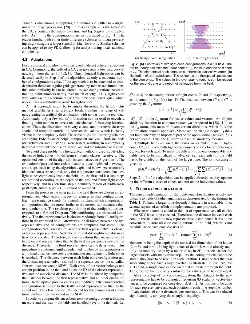
In order to compute distances between two configurations a distancemeasure and the way multifields are handled have to be defined. Let
(a) Sample cone configuration (b) Iterated light-cones
Fig. 2. (a) Illustration of two light-cone configurations in a 1D field. Thered boundary encloses the future cone of T0, the blue one the past coneof T0. The elements of each cone are numbered in successive order. (b)Illustration of an iterated cone. The red cones are the spatial successorsof the blue ones. The values in the overlapping regions can be reusedfor the second cone and need not be loaded from the field.
S0i and S1
i be the configurations of light-cones C0 and C1 respectively,
as illustrated in Fig. 2(a) for 1D. The distance between C0 and C1 isgiven by the L2-norm:
‖C0−C1‖=√
∑i
‖S0i −S1
i ‖2 (6)
‖S0i − S1
i ‖ is the L2-norm for scalar values and vectors. An ellipticsimilarity function to compare vectors was proposed in [38]. Unlikethe L2-norm, this measure favors certain directions, which foils theinformation theoretic approach. Moreover, the triangle inequality doesnot hold, whereby an important part of the optimization (see Sec. 5) isnot applicable. Thus, the L2-norm is taken as similarity measure.
If multiple fields are used, the cones are extended to multi light-cones MC, i.e., each multi light-cone consists of a vector of light-conesC j, one for each field. To make the different subcones comparable, thefields have to be normalized in advance, i.e., each entry in the fieldhas to be divided by the norm of the largest one. The joint distance isgiven by
‖MC0−MC1‖=√
∑j
‖C0j −C1
j ‖2 =
√
∑j∑
i
‖S0i j−S1
i j‖2 (7)
Steps 2 to 4 of the algorithm can be applied directly, as they operateon the different classes of cones, and not on the individual values.
5 EFFICIENT IMPLEMENTATION
The naive implementation of the light-cone classification is only ap-plicable to fields of rather small size as demonstrated by the timings inTable 1. To handle larger time-dependent datasets in reasonable time,several aspects of an efficient implementation are proposed.
Whenever a cone is added to the list of representatives, all entriesin the SDV have to be checked. Therefore, the distance between eachcone in the field and the new representative is computed. It would beconvenient to store all cone configurations in the field, which is notpossible, since each cone consists of
past:n−1
∑i=0
(3+2i)d future:n−1
∑i=0
(1+2i)d (8)
elements, n being the depth of the cone, d the dimension of the lattice(2 or 3), and c = 1. Using light-cones of depth 3, would already mul-tiply the memory usage by a factor of 83 in 2D, a crucial factor forlarge datasets with many time steps. As the configurations cannot bestored, they have to be rebuilt in each iteration. Using the fact that twosucceeding cones have a large overlap, as illustrated in Fig. 2(b) fora 1D field, a single cone can be used that is iterated through the field.Thus, most of the time only a subset of the values has to be exchanged.
After the setup of the cone configuration, the distance to the newrepresentative has to be computed, requiring 83 scalar or vector dis-tances to be computed for cone depth 3, d = 2. As this has to be donefor each representative and each position in each time step, the numberof calculations of cone distances gets enormous. This can be reducedsignificantly by applying the triangle inequality.
‖rc− rn‖ ≤ ‖l− rc‖+‖l− rn‖ (9)
Algorithm 1 Classification of light-cones
The field to be analysed is defined on a regular grid ofnbXPos×nbYPos positions, and nbTimeSteps time steps.pastDepth← depth of past light-conesfutureDepth← depth of future light-conesoffset← max( pastDepth, futureDepth - 1 )· cn← ( nbXPos - 2·offset ) · ( nbYPos - 2·offset ) ·
( nbTimeSteps - pastDepth - ( futureDepth - 1 ))
r← randomly chosen representativeadd r to the list of representativesfor i = 1 . . . n do
SDV[i]← distance between r and the ith light-conerepresentative[i]← 0
end forinit the list of candidates
while stopCriterion not fulfilled doif SDV[lastCandidate] > maxExcludedDist then
add lastCandidate to the list of representativesupdate the distances of the candidates
elseupdate the SDVcompute a new list of candidates
end ifend whileupdate the SDV
The inequality compares the three distances between the followingcone configurations: the current light-cone (l), the closest represen-tative (rc), and the new representative (rn): Thus, the new repre-sentative can only be closer to the configuration than the old one(‖l− rn‖< ‖l− rc‖) if Eq. 10 holds.
‖rc− rn‖< 2‖l− rc‖ (10)
To employ this property, a matrix of all inter-representative distancesis stored. Entry (i, j) of the matrix stores the distance between rep-resentatives i and j. Whenever a new representative is selected, anadditional row and column has to be added to the matrix. Thus, bothquantities of Eq. 10 are computed only once. ‖rc− rn‖ is store in thematrix and ‖l− rc‖ in the SDV. The costly computation of the newdistance ‖l− rn‖ is only performed if Eq. 10 holds. Thus, many com-parisons can be omitted at very low cost.
So far, new representatives are chosen from all configurations inthe field, although there are many configurations that are very similarto earlier defined representatives. Note that distances in the SDV canonly become shorter by adding new representatives. If new represen-tatives were chosen only from the configurations most dissimilar to se-lected representatives, the costs for the update can be further reduced.Accordingly, a list of potential representatives is stored. From the SDVthe n cones with the longest distances are identified and their configu-rations and minimal distances are stored in a seperate list. n is a valuespecified by the user, e.g., if 3000 representatives are to be detected,lists of 600 cones were used. As an optimal choice of n depends highlyon the dynamics of the field, no optimal value can be predefined. Ad-ditionally, the worst excluded distance is stored, which is the n + 1stlongest distance in the SDV. The iteration now only operates on the listof potential representatives. Whenever a new representative is added,only the minimal distances of the candidates are updated, which re-duces the number of updates in a dataset with 100,000 positions from100,000 to 600. Afterwards, a new representative is chosen from thelist. This procedure is continued until the worst distance in the can-didate list is shorter than the worst excluded one. As distances canonly become shorter by adding new candidates, the worst excludeddistance cannot become larger. For the given example of list length600 approximately 150 representatives were added, before a new listhad to be computed.
All improvements explained so far do not change the results, as theyare just more efficient techniques and no heuristics. Nevertheless, forlong time series the computational effort might still be too large. Todecrease workload, the cone classification can be reduced to a subsetof time-steps, i.e., representatives are chosen from every ith time-step.If the configurations in the field change at moderate speed, no essentialstructures are missed. The intermediate time-steps are classified in asecond step. Again, the triangle inequality can be used to identify theclosest representative. The shortest representative from the previoustime-step is taken as an estimation of the shortest distance. From thelist of representatives only those are compared to the current light-cone, that fulfill Eq. 10.
6 RESULTS AND DISCUSSION
6.1 Influence of the Parameters
The computation of the causal states depends on two parameters: thedepth of the light cones, and the number of representatives. The “Flowaround a cylinder” (Section 6.5) is used to illustrate their influence.
Fig. 8 shows the complexity fields for different light-cone depths.The complexity field for the minimal configurations with past depth 1and future depth 2 is shown in the third image. It already captures allrelevant structures. Increasing the past depth to 2 results in smootherstructures, as the region of influence becomes larger and single devia-tions are evened out. The difference between the two fields is shownin the fifth image. Blue regions indicate a higher complexity in the im-age with the smaller cones, red regions higher complexity in the imagewith deeper cones. The difference field is quite homogeneous, reveal-ing the uniform modification of the field. Cones of depth 6 are usedin the second image, which appears smoother than the other two. Thedifference field gives the same results as in the previous case. Thus,the depth of the cones has no significant influence on the result. Thedeeper the cones the smoother the image. To decrease computationalcosts, cones of depth 2 were chosen for all examples.
Just as the depth of light-cones, the number of representatives hasno significant influence on the results. Fig. 6 shows the same datasetwith different numbers of representatives used in the computation ofcomplexity. If too few representatives are computed the relevant struc-tures are visible but poorly developed. In the case of 8000 representa-tives certain regions are overrepresented, resulting in a kind of overfit-ting. Visually best results could be achieved when limiting the numberof representatives to approximately 5000. Thus, the choice of the pa-rameters has no great influence on the qualitative results, they mainlydetermine the quality of the resulting images.
6.2 Isotropic Diffusion
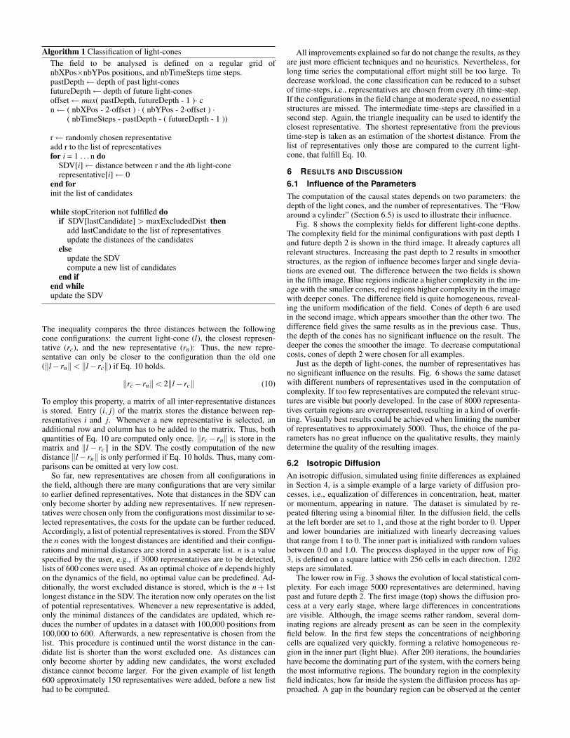
An isotropic diffusion, simulated using finite differences as explainedin Section 4, is a simple example of a large variety of diffusion pro-cesses, i.e., equalization of differences in concentration, heat, matteror momentum, appearing in nature. The dataset is simulated by re-peated filtering using a binomial filter. In the diffusion field, the cellsat the left border are set to 1, and those at the right border to 0. Upperand lower boundaries are initialized with linearly decreasing valuesthat range from 1 to 0. The inner part is initialized with random valuesbetween 0.0 and 1.0. The process displayed in the upper row of Fig.3, is defined on a square lattice with 256 cells in each direction. 1202steps are simulated.
The lower row in Fig. 3 shows the evolution of local statistical com-plexity. For each image 5000 representatives are determined, havingpast and future depth 2. The first image (top) shows the diffusion pro-cess at a very early stage, where large differences in concentrationsare visible. Although, the image seems rather random, several dom-inating regions are already present as can be seen in the complexityfield below. In the first few steps the concentrations of neighboringcells are equalized very quickly, forming a relative homogeneous re-gion in the inner part (light blue). After 200 iterations, the boundarieshave become the dominating part of the system, with the corners beingthe most informative regions. The boundary region in the complexityfield indicates, how far inside the system the diffusion process has ap-proached. A gap in the boundary region can be observed at the center

of the upper and lower boundary region. In these parts, the constantgradient on the boundary already has the average value of 0.5. Severaldominant regions can be distinguished in the inner part, being relevantup to the final step. The two images of time step 1200 illustrate verywell, that not only the propagating front of diffusion is important, butthe whole strip starting from the boundary.
6.3 Local Statistical Complexity of CFD Datasets
The diffusion example perfectly matches the requirements of themethod, but is rather trivial from an application point of view. Whenanalysing simulations from the field of fluid dynamics, local statisticalcomplexity has to be applied carefully.
Many computational fluid dynamic (CFD) datasets are solutions tothe Navier-Stokes Equations for incompressible flow:
∂
∂ t~u+(~u ·∇)~u+∇p =
1
Re∆~u+~g (11)
∇ ·~u = 0 (12)
where ~u is the velocity, p is the pressure, ~g are body forces, and Reis the Reynolds number [14]. In incompressible flow, density is as-sumed to be constant, ρ(~x, t) = ρ∞ = const. When simulating a fluidusing these equations, pressure is used to ensure, that divergence is 0,i.e., Eq. 12 holds. Therefore, in each iteration of the simulation, thepressure is adapted all over the field, whereby pressure is no longer alocal quantity, and c = ∞ for the light-cones. Thus, the cones wouldhave to comprise the whole field in order to capture all informationaffecting the current position. Analyzing only the velocity by meansof local statistical complexity, neglects important information, as ve-locity and pressure are coupled variables. Hence, an exact solution toincompressible flow systems is not possible using the current method.In Sec. 6.5 the complexity fields of velocity, pressure, and of velocityand pressure are analysed. While the investigation of the individualfields is incomplete, the analysis of both fields gives very good ap-proximations of the relevant structures even with small cones (c = 1)for pressure. An alternative approach is to use the vorticity, which isnot influenced by the pressure. Examples of both approaches will beshown in the following two sections in context.
It should be noted that this restriction holds only for incompressibleflow simulations. Finite difference simulations of compressible flowfit perfectly the requirements of local statistical complexity analysis.
6.4 Swirling Flow
The development of a recirculation zone in a swirling flow is investi-gated by numerical simulation. This type of flow is relevant to severalapplications where residence time is important to enable mixing andchemical reactions.
The unsteady flow in a swirling jet is simulated with an accuratefinite-difference method. The Navier-Stokes equations for an incom-pressible, Newtonian fluid are set up in cylindrical coordinates assum-ing axi-symmetry in terms of streamfunction and azimuthal vorticity.All equations are dimensionless containing the Reynolds number Reand the swirl number S as defined by Billant et al. [6]
Re≡vz(0,z0)D
νS≡
2vθ (R/2,z0)
vz(0,z0)(13)
where z0 = 0.4D, D = 2R is the nozzle diameter and ν the kinematicviscosity, as dimensionless parameters.
The PDEs are discretized with fourth order central difference opera-tors for the non-convective terms and with a fifth order, upwind-biasedoperator [26] for the convective terms. The time integrator is an ex-plicit s-stage, state space Runge-Kutta method ([8], [21]), the presentmethod is fourth order accurate with s = 5. The time step is controlledby the minimum of two criteria: The limit set by linearized stabilityanalysis and the limit set by the error norms of an embedded third or-der Runge-Kutta scheme [8]. The Helmholtz PDE for streamfunctionΨ(r,z, t) is solved with an iterative method using deferred corrections
12.0
6.0
0.0
1.0
0.5
0.0
Fig. 3. An isotropic diffusion with fixed concentrations at the boundaries,inducing a gradient from the left to the right handside. The upper rowshows the concentrations at time step 2, 200, 500, and 1200. Regionsof high importance for the system’s dynamics, extracted using local sta-tistical complexity, are displayed in the lower row.
and LU-decomposition of the coefficient matrix. The deferred correc-tions method is designed to reduce the bandwidth of the coefficientmatrix. It converges rapidly using about ten to twenty steps.
The flow domain is the meridional plane D = {(r,z) : 0≤ r≤R,0≤z≤ L} with R = 5D, L = 8D and D denoting the nozzle diameter at theentrance boundary. The flow domain is mapped onto the unit rectanglewhich is discretized with constant spacing. The mapping is separableand allows to a limited extent crowding of grid points in regions of in-terest. The present simulation uses nr = 91 and nz = 175 grid points inradial and axial directions. The boundary conditions are of Dirichlettype at the entrance section and the outer boundary and at the exit con-vective conditions are imposed for the azimuthal vorticity. The initialconditions are stagnant flow and the entrance conditions are smoothlyramped up to their asymptotic values within four time units.
The simulation results for Re = 103, S = 1.1 (within the range of theexperiments [6], [27]) used for the complexity analysis are ten timesteps after the formation of the recirculation bubble (which forms att = 6.02) at times t = 33.63092 to t = 33.70560. The flow is unsteadyand does not approach a steady asymptotic state as the velocity andvorticity fields show (Fig. 4(top)). Fig. 4(top/left) shows a LIC of thevelocity field, featuring several vortices. When overlayed with a trans-parent map, hiding regions of very low velocity, a better impression ofthe flow is provided, as many vortices are detected in regions close tonoise. Local statistical complexity is computed for velocity and vortic-ity separately (Fig. 4(bottom/ middle and right)), and for both fields ata time (Fig. 4(bottom/left)). The main structures that have developedup to the instant of the analysis are a conical shear region, outlinedin blue in Fig. 4(top/left), and several ringlike vortex structures, onebeing marked with red points in Fig. 4(top/left). Both features aredetected by local statistical complexity. Only minor differences ex-ist between the analysis of velocity, vorticity, and the combination ofboth fields. This might be due to the fact, that the system’s dynamicsare quite complex. Thus, it is easier to distinguish between regions,where it is difficult to predict the system’s future dynamics, and thosewhere it is easy. As this differentiation is quite clear, it is present inboth fields. Unlike vorticity, local statistical complexity marks bothfeatures as equally complex. Both, the conical shear region, as well asthe vortex structure are assigned highest complexity, while the vorticesexhibit only small vorticity, compared to the shear flow.
6.5 Flow Around a Cylinder
The flow around a cylinder is a widely researched and well understoodproblem in fluid mechanics. Over a certain range of Reynolds num-bers, the flow becomes asymmetric and unsteady, forming the wellknown von Karman vortex street [14]. The flow is simulated usingNaSt2D, the solver explained in [14], and available online at [10]. Theconfiguration file for a flow around a cylinder provided with the im-plementation is used for the simulation, ensuring correct settings. Thegrid consists of 660×120 positions. 4500 time steps are simulated,ranging from times t = 0.0 to t = 44.53. The simulation output con-sists of three fields: velocity, pressure, and vorticity, which are visual-ized for time step 3402 in Fig. 7.

0.2
0.0
0.1
1.0
0.05
0.525
7.15
-7.15
0.0
10.4
6.0
8.2
10.4
6.0
8.2
10.4
6.0
8.2
Fig. 4. (top) Illustrations of the swirling flow: (left) (left)LIC of the velocity of the swirling flow. The conical shear region is outlined in blue. Severalringlike vortex structures can be observed, one being marked by red points. (right) The LIC is overlayed by a transparent mask, hiding regions ofsmall velocity. Thus, the structure of the flow is clarified. (middle) Norm of the velocity. (right) Vorticity.(bottom) Local statistical complexity fields of the swirling flow from left to right: velocity and vorticity, velocity, vorticity.
The corresponding local statistical complexity fields are displayedin Fig. 9. As stated earlier, the presented method cannot be directlyapplied to the pressure. Fig. 9(top) shows the complexity of the pres-sure, using light-cones with c = 1. It is clearly visible, that the analysislacks information, as the structures are no longer continuous and fea-ture holes. The complexity field of the velocity (Fig. 9(second)), high-lights the important structures in the flow. Most dominant is the re-gion, where the flow hits the object, stretching to the seperation struc-tures behind the cylinder. The region where vortices originate is alsomarked in dark blue, as well as the current positions of vorticies in thevortex street. A ribbon shaped like a sinus runs through the whole vor-tex street, linking the periodically created vortices. The complex re-gions at the top and bottom mark regions of shear flow, induced by theboundaries. In general, the complexity field of the vorticity exhibitsthe same structures. Nevertheless, in both images the structures arenot fully developed, as information is missing. Fig. 9(bottom) showsthe complexity of all three fields. As more information is included inthis analysis, the relevant regions get more dominant and smoother.
The fifth image in Fig. 7 shows the λ2-field of the current time step.The λ2 criterion is a standard technique to visualize vortices [32]. Avortex is defined as the region where λ2 < 0. Thus, the blue regions inFig. 7 (bottom) are of relevance, featuring the position of the vorticesin the von Karman vortex street, the regions of separation at both sidesof the cylinder, and the shear flow at the boundary. The positions of thevortices match perfectly the regions of highest complexity in the sinusshaped ribbon. The major advantages of λ2 and vorticity plots are itsshort computation times (only a few seconds). As long as the flow’sdynamic is rather simple, these methods are more advantageous. Thewell known and simple examples were chosen to prove the correctnessof local statistical complexity. To tap its full potential, more compli-cated flows are needed that are often simulated on unstructured gridsthat cannot be analysed so far. An advantage of complexity analysisis the fact that it shows smoother structures, providing a good context.The interaction of the flow behind the cylinder is more clearly repre-sented by local statistical complexity, as the system is considered as aunity and not seperated into different classes of behavior, as done bythe λ2-criterion and vorticity.
6.6 Weather and Climate
In order to test the method also with data with more complex statis-tical properties, we have chosen data from a global climate simula-tion done by the Max Planck-Institute for Meteorology (MPI-M) atthe German Climate Computing Center (DKRZ). The data was ac-quired from the ”World Data Center for Climate” (WDCC) database.Due to time constraints we have selected a subset of only one simu-lated year and 15 surface variables of the atmospheric component of
the coupled atmosphere-ocean-model ECHAM / MPI-OM [31]. Witha time resolution of 6 hours the data includes the daily cycle. Thespatial resolution is approximately 200 km.
Fig. 7(top) shows the wind and the evaporation of timestep 247.The combination of both fields shows that a visual analysis is ratherdifficult as the system is quite complex and no simple structures attractattention. When analyzing these two fields with local statistical com-plexity several dominant regions appear (Fig. 7(bottom)). Timings aregiven in Table 1. A region well known for its high spatio-temporalvariability is the north atlantic area. Storm systems often develop inthe western part of the atlantic, and many of them move across thenorth atlantic towards europe. Storm activity is highly correlated withwindspeed and other meteorological parameters like vorticity, precipi-tation and evaporation. Due to the chaotic behavior of the weather andclimate system, the deterministic forecast of storm tracks for a coupleof days is still a scientific challenge. Our method highlights especiallythose features of the weather system which occur irregularly and henceare difficult to forecast.
The video shows the temporal development of wind and evapora-tion. The diurnal cycle of evaporation is clearly visible. In a long-termanalysis using local statistical complexity this regularity should be de-tected and classified as little complex. As can be seen in the complex-ity video of the weather, the current method is not capable of filteringthese events, as there are too large fluctuations in the daily curves. Thedetection of regular events will be part of future work.
7 CONCLUSION AND FUTURE WORK
In this paper, local statistical complexity is introduced, as a methodto detect important regions in systems that can be described by PDEs.Four examples are used to illustrate the new technique, which detectscrucial structures in the system automatically. Unlike most feature de-tection methods, local statistical complexity does not rely on specifi-cations given by the users, but estimates complexity from the system’sdynamics. Thus, the technique is perfectly suited to investigate sys-tems that are only little understood, and give hints, where to look forimportant regions. The interpretation of complexity becomes increas-ingly difficult as more variables are included. Hence, the complexityanalysis of the weather simulation is executed with only two variables.Research towards a better understanding of the interactions of severalvariables and their effect on the complexity field will be subject offuture work.
ACKNOWLEDGEMENTS
The authors wish to thank the developers of NaST2D for making theprogram publically available. Special thanks go to Michael Bottingerfor providing the weather simulation and for many helpful remarks.
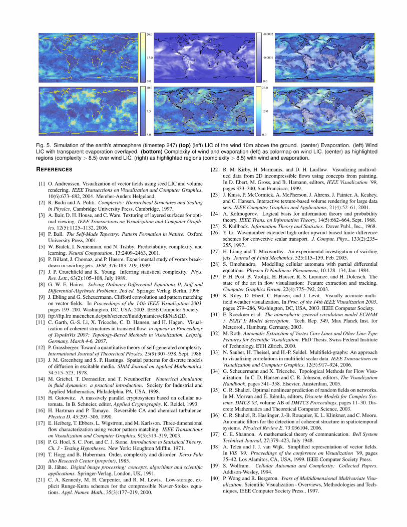
26.0
13.0
0.0 0.0
-0.0002
-0.0001
10.0
7.5
5.0
26.0
13.0
0.0
Fig. 5. Simulation of the earth’s atmosphere (timestep 247) (top) (left) LIC of the wind 10m above the ground. (center) Evaporation. (left) WindLIC with transparent evaporation overlayed. (bottom) Complexity of wind and evaporation (left) as colormap on wind LIC. (center) as highlightedregions (complexity > 8.5) over wind LIC. (right) as highlighted regions (complexity > 8.5) with wind and evaporation.
REFERENCES
[1] O. Andreassen. Visualization of vector fields using seed LIC and volume
rendering. IEEE Transactions on Visualization and Computer Graphics,
10(6):673–682, 2004. Member-Anders Helgeland.
[2] R. Badii and A. Politi. Complexity: Hierarchical Structures and Scaling
in Physics. Cambridge University Press, Cambridge, 1997.
[3] A. Bair, D. H. House, and C. Ware. Texturing of layered surfaces for opti-
mal viewing. IEEE Transactions on Visualization and Computer Graph-
ics, 12(5):1125–1132, 2006.
[4] P. Ball. The Self-Made Tapestry: Pattern Formation in Nature. Oxford
University Press, 2001.
[5] W. Bialek, I. Nemenman, and N. Tishby. Predictability, complexity, and
learning. Neural Computation, 13:2409–2463, 2001.
[6] P. Billant, J. Chomaz, and P. Huerre. Experimental study of vortex break-
down in swirling jets. JFM, 376:183–219, 1999.
[7] J. P. Crutchfield and K. Young. Inferring statistical complexity. Phys.
Rev. Lett., 63(2):105–108, July 1989.
[8] G. W. E. Hairer. Solving Ordinary Differential Equations II, Stiff and
Differential-Algebraic Problems, 2nd ed. Springer Verlag, Berlin, 1996.
[9] J. Ebling and G. Scheuermann. Clifford convolution and pattern matching
on vector fields. In Proceedings of the 14th IEEE Visualization 2003,
pages 193–200, Washington, DC, USA, 2003. IEEE Computer Society.
[10] ftp://ftp.lrz muenchen.de/pub/science/fluiddynamics/cfd/NaSt2D.
[11] C. Garth, G.-S. Li, X. Tricoche, C. D. Hansen, and H. Hagen. Visual-
ization of coherent structures in transient flow. to appear in Proceedings
of TopoInVis 2007: Topology-Based Methods in Visualization, Leipzig,
Germany, March 4-6, 2007.
[12] P. Grassberger. Toward a quantitative theory of self-generated complexity.
International Journal of Theoretical Physics, 25(9):907–938, Sept. 1986.
[13] J. M. Greenberg and S. P. Hastings. Spatial patterns for discrete models
of diffusion in excitable media. SIAM Journal on Applied Mathematics,
34:515–523, 1978.
[14] M. Griebel, T. Dornseifer, and T. Neunhoeffer. Numerical simulation
in fluid dynamics: a practical introduction. Society for Industrial and
Applied Mathematics, Philadelphia, PA, USA, 1998.
[15] H. Gutowitz. A massively parallel cryptosystem based on cellular au-
tomata. In B. Schneier, editor, Applied Cryptography. K. Reidel, 1993.
[16] H. Hartman and P. Tamayo. Reversible CA and chemical turbulence.
Physica D, 45:293–306, 1990.
[17] E. Heiberg, T. Ebbers, L. Wigstrom, and M. Karlsson. Three-dimensional
flow characterization using vector pattern matching. IEEE Transactions
on Visualization and Computer Graphics, 9(3):313–319, 2003.
[18] P. G. Hoel, S. C. Port, and C. J. Stone. Introduction to Statistical Theory:
Ch. 3 - Testing Hypotheses. New York: Houghton Mifflin, 1971.
[19] T. Hogg and B. Huberman. Order, complexity and disorder. Xerox Palo
Alto Research Center (preprint), 1985.
[20] B. Jahne. Digital image processing: concepts, algorithms and scientific
applications. Springer-Verlag, London, UK, 1991.
[21] C. A. Kennedy, M. H. Carpenter, and R. M. Lewis. Low-storage, ex-
plicit Runge-Kutta schemes for the compressible Navier-Stokes equa-
tions. Appl. Numer. Math., 35(3):177–219, 2000.
[22] R. M. Kirby, H. Marmanis, and D. H. Laidlaw. Visualizing multival-
ued data from 2D incompressible flows using concepts from painting.
In D. Ebert, M. Gross, and B. Hamann, editors, IEEE Visualization ’99,
pages 333–340, San Francisco, 1999.
[23] J. Kniss, P. McCormick, A. McPherson, J. Ahrens, J. Painter, A. Keahey,
and C. Hansen. Interactive texture-based volume rendering for large data
sets. IEEE Computer Graphics and Applications, 21(4):52–61, 2001.
[24] A. Kolmogorov. Logical basis for information theory and probability
theory. IEEE Trans. on Information Theory, 14(5):662–664, Sept. 1968.
[25] S. Kullback. Information Theory and Statistics. Dover Publ., Inc., 1968.
[26] Y. Li. Wavenumber-extended high-order upwind-biased finite-difference
schemes for convective scalar transport. J. Comput. Phys., 133(2):235–
255, 1997.
[27] H. Liang and T. Maxworthy. An experimental investigation of swirling
jets. Journal of Fluid Mechanics, 525:115–159, Feb. 2005.
[28] S. Omohundro. Modelling cellular automata with partial differential
equations. Physica D Nonlinear Phenomena, 10:128–134, Jan. 1984.
[29] F. H. Post, B. Vrolijk, H. Hauser, R. S. Laramee, and H. Doleisch. The
state of the art in flow visualisation: Feature extraction and tracking.
Computer Graphics Forum, 22(4):775–792, 2003.
[30] K. Riley, D. Ebert, C. Hansen, and J. Levit. Visually accurate multi-
field weather visualization. In Proc. of the 14th IEEE Visualization 2003,
pages 279–286, Washington, DC, USA, 2003. IEEE Computer Society.
[31] E. Roeckner et al. The atmospheric general circulation model ECHAM
5. PART I: Model description. Tech. Rep. 349, Max Planck Inst. for
Meteorol., Hamburg, Germany, 2003.
[32] M. Roth. Automatic Extraction of Vortex Core Lines and Other Line-Type
Features for Scientific Visualization. PhD Thesis, Swiss Federal Institute
of Technology, ETH Zurich, 2000.
[33] N. Sauber, H. Theisel, and H.-P. Seidel. Multifield-graphs: An approach
to visualizing correlations in multifield scalar data. IEEE Transactions on
Visualization and Computer Graphics, 12(5):917–924, 2006.
[34] G. Scheuermann and X. Tricoche. Topological Methods for Flow Visu-
alization. In C. D. Hansen and C. R. Johnson, editors, The Visualization
Handbook, pages 341–358. Elsevier, Amsterdam, 2005.
[35] C. R. Shalizi. Optimal nonlinear prediction of random fields on networks.
In M. Morvan and E. Remila, editors, Discrete Models for Complex Sys-
tems, DMCS’03, volume AB of DMTCS Proceedings, pages 11–30. Dis-
crete Mathematics and Theoretical Computer Science, 2003.
[36] C. R. Shalizi, R. Haslinger, J.-B. Rouquier, K. L. Klinkner, and C. Moore.
Automatic filters for the detection of coherent structure in spatiotemporal
systems. Physical Review E, 73:036104, 2006.
[37] C. E. Shannon. A mathematical theory of communication. Bell System
Technical Journal, 27:379–423, July 1948.
[38] A. Telea and J. J. van Wijk. Simplified representation of vector fields.
In VIS ’99: Proceedings of the conference on Visualization ’99, pages
35–42, Los Alamitos, CA, USA, 1999. IEEE Computer Society Press.
[39] S. Wolfram. Cellular Automata and Complexity: Collected Papers.
Addison-Wesley, 1994.
[40] P. Wong and R. Bergeron. Years of Multidimensional Multivariate Visu-
alization. Scientific Visualization - Overviews, Methodologies and Tech-
niques, IEEE Computer Society Press., 1997.

Table 1. Timings for Isotropic Diffusion (Diffusion), Swirling Flow (Swirl), Flow Around a Cylinder (Cylinder), and Weather (weather). The followingabbreviations are used: the different Fields used for the analysis are vector (v) or scalar (s) valued; the different Implementations used are simple(none of the efficient implementation strategies is used), or efficient (all strategies are used); Past and Future Depth denote the depth of the pastand future light-cones respectively; # Representatives is the number of representative used in the classification process; Size of List gives thenumber of candidates in the classification; # Omitted denotes the number of time steps being omitted, when classifying the representatives.
Dataset Fields Implementation Past Depth Future Depth # Representatives Size of List # Time Steps # Omitted Time
Cylinder 2s, 1v simple 3 3 200 - 5 0 1 h 20 min
Cylinder 2s, 1v efficient 3 3 200 700 5 0 14 min
Cylinder 2s, 1v efficient 2 2 5000 1 1 0 58 min
Cylinder 2s, 1v efficient 2 2 5000 700 1 0 12 min
Cylinder 2s, 1v efficient 2 2 9000 700 300 20 4h 5min
Swirl 1s, 1v efficient 2 2 5000 600 1 0 6 min
Diffusion 1s efficient 2 2 5000 600 1 0 4 min
Weather 2s efficient 3 3 4000 1000 1 0 14 min
16.25
9.5
3.0
16.25
11.0
6.0
16.25
11.0
6.0
16.25
11.0
6.0
16.25
11.0
6.0
Fig. 6. The complexity field of the flow around a cylinder (time step3402) with different numbers of representatives. From top to bottom:200, 1000, 2000, 5000, 8000.
1.8
0.9
0.0
1.5
0.0
-0.7
18.5
0.0
-18.5
Fig. 7. Flow around a cylinder: The images are a snapshot at timet = 33.637066 (time step 3402). The first and second image display thevelocity using LIC and a colorcoding of the norm of the velocity. Thethird image shows pressure, the fourth vorticity, and the fifth λ2.
16.25
11.0
6.0
16.25
11.0
6.0
16.25
11.0
6.0
Fig. 8. The complexity field of the flow around a cylinder (time step3402) with different depths of the cones. From top to bottom (past depth/future depth): difference between (6/6) and (1/2), complexity for (6/6),complexity for (1/2), complexity for (2/2), difference between (2/2) and(1/2)
16.25
11.0
6.0
16.25
11.0
6.0
16.25
11.0
6.0
16.25
11.0
6.0
Fig. 9. Complexity fields of the flow around a cylinder (time step 3402)from top to bottom: Pressure, velocity, vorticity, pressure and velocityand vorticity. For all computations parameters are chosen as follows:depth of past and future cones 2, number of representatives in clas-sification 5000, size of candidate list in classification 600, number oftime-steps 1