Multidisciplinary Design Optimization of a Novel Sandwich

materials

Article

Multidisciplinary Design Optimization of a NovelSandwich Beam-Based Adaptive Tuned VibrationAbsorber Featuring Magnetorheological Elastomer

Mostafa Asadi Khanouki, Ramin Sedaghati * and Masoud Hemmatian

Department of Mechanical, Industrial and Aerospace Engineering, Concordia University,Montreal, QC H3G 1M8, Canada; [email protected] (M.A.K.);[email protected] (M.H.)* Correspondence: [email protected]

Received: 25 April 2020; Accepted: 9 May 2020; Published: 14 May 2020��

Abstract: The present study aims to investigate the dynamic performance and design optimizationof a novel magnetorheological elastomer based adaptive tuned vibration absorber (MRE-ATVA).The proposed MRE-ATVA consists of a light-weight sandwich beam treated with an MRE corelayer and two electromagnets installed at both free ends. Three different design configurationsfor electromagnets are proposed. The finite element (FE) model of the proposed MRE-ATVA andmagnetic model of the electromagnets are developed and combined to evaluate the frequency rangeof the absorber under varying magnetic field intensity. The results of the developed model arevalidated in multiple stages with available analytical and simulation data. A multidisciplinarydesign optimization strategy has been formulated to maximize the frequency range of the proposedMRE-based ATVA while respecting constraints of weight, size, mechanical stress, and sandwichbeam deflection. The optimal solution is obtained and compared for the three proposed ATVAconfigurations. The optimal ATVA with a U-shaped electromagnet shows more than 40% increase inthe natural frequency while having a total mass of 596 g.

Keywords: multidisciplinary design optimization; magnetorheological elastomers; adaptive tunedvibration absorber; smart sandwich beam

1. Introduction

Magnetorheological elastomer (MRE) is a functional material which responds to an appliedmagnetic field by changing its viscoelastic properties. MREs are basically the solid analog ofmagnetorheological fluids (MRFs) as they are composed of micron-sized ferromagnetic particles,typically carbonyl iron powder dispersed into a nonmagnetic solid polymeric or elastomericmedium such as silicone rubber. MREs overcome the problems that accompany the applications ofmagnetorheological (MR) fluids, such as sedimentation of particles, sealing issues, and environmentalcontamination. The magnetic properties of MREs originate from microstructural interactions under amagnetic field and depend on different parameters such as volume fraction and spatial distribution ofembedded ferromagnetic particles [1–3]. When exposed to an external magnetic field, MRE changesits dynamic properties, including both stiffness and damping, rapidly and reversibly, thus, making itan ideal candidate for the development of the next generation of adaptive devices with controllableoperating frequency and damping [4].

One intriguing application of MREs is in the development of adaptive vibration absorbers whichcan be effectively utilized to attenuate vibration in a broad range of frequencies. To date, severaldesigns have been proposed in the literature for vibration absorbers featuring MREs. Lerner and

Materials 2020, 13, 2261; doi:10.3390/ma13102261 www.mdpi.com/journal/materials

http://www.mdpi.com/journal/materials

http://www.mdpi.com

https://orcid.org/0000-0002-8323-1474

http://www.mdpi.com/1996-1944/13/10/2261?type=check_update&version=1

http://dx.doi.org/10.3390/ma13102261

http://www.mdpi.com/journal/materials

Materials 2020, 13, 2261 2 of 22

Cunefare [5] designed three types of MRE-based vibration absorbers working in shear, squeeze,and longitudinal modes, and among these, the squeeze mode absorber exhibited the widest frequencyrange. Sun et al. [6] designed and prototyped a squeeze working mode MRE-based absorber thatdemonstrated a frequency range of 37 to 67 Hz by providing magnetic field intensity ranging from 0 to250 kA/m. There are also other important research studies that have investigated the application ofMREs in adaptive vibration absorbers [7–9]; however, one important task in the development of efficientMRE-based absorbers is the optimization of these smart devices to achieve the best performance.

There have been efforts that considered the analysis and optimal design of MR dampers andabsorbers. Parlak et al. [10] carried out optimization on an MR damper’s geometry pursuing twoobjectives of target damper force and maximum magnetic flux density. They used finite element-basedelectromagnetic and CFD tools of ANSYS to perform the optimization. Nguyen and Choi [11] proposedan optimal design for a passenger vehicle MR damper which was constrained in a specific volume.The objective function involved damping force, the dynamic range, and inductive time constant ofthe damper. In recent years, there have also been a number of studies that investigated the designoptimization of rotary and translational MR-based dampers and absorbers [12–14]. Nevertheless,research studies that analyze MR vibration absorber devices which have continuous structures such asbeams are very limited. Particularly, there have been no study conducted on the development of designoptimization strategies for such adaptive devices. Hirunyapruk et al. [15] proposed a three-layerbeam-like tuned vibration absorber which was treated with MRF in the core layer. Two electromagnetswere considered on the beam to apply a magnetic field on the MRF layer. One unique feature of thesandwich beam with treated MR fluid core layers is that the stiffness of the beam and, subsequently,its natural frequencies can be continuously changed by activating the MR fluid. Hirunyapruk et al.demonstrated that the natural frequency of the device could change from 106 to 149 Hz [15]. While thiswork is very useful for demonstrating the feasibility and operation of beam-like absorber devices,the optimal design problem of the absorber has not been addressed. To the best of our knowledge,there have been no study conducted on the development and multidisciplinary design optimization ofadaptive vibration absorbers featuring multilayer MRE-based sandwich structures.

Consequently, the main contribution of this work is, first, to propose three different novelconfigurations for an MRE-based sandwich beam type adaptive tuned vibration absorber (MRE-ATVA)and, then, to propose a multidisciplinary optimization framework to maximize their frequencybandwidth. To this end, the comprehensive models of the proposed MRE-ATVAs are developed whichconsists of the following two components: the finite element (FE) model of the sandwich beam, and themathematical formulation for magnetic analysis of the electromagnets. The MRE in the core layer ofthe sandwich beam operates in shear mode, and thus its shear modulus changes under the appliedmagnetic field generated by the electromagnets installed at the tips of the beam. Thus, the naturalfrequency of the absorber can be continuously varied and controlled through the application of therequired magnetic field. The electromagnets on the beam ends play a two-fold role by providing therequired magnetic field on the MRE layer, as well as oscillating as the absorber mass. Three differentdesign configurations are considered for the electromagnets to have insights on the flexible design ofthe proposed absorber device. Then, using the developed model of the absorber, a multidisciplinaryoptimal design problem which considers both the structural geometry and electromagnet parametersas design variables, is formulated aiming at maximizing the frequency range of the absorber, respectingconstraints on the total mass, static deflection, and maximum stress in the beam. To accurately identifythe optimal design, the optimization problem is solved using a combination of genetic algorithm (GA)and powerful sequential quadratic programming (SQP) methods. Then, the identified optimal designsfor the proposed MRE-ATVAs are compared and discussed.

In this paper, first, the configuration of the proposed MRE-ATVAs with three potential designs ofthe electromagnet are introduced. Secondly, the FE model of the sandwich beam and magnetic modelof the electromagnets are developed and validated. By integrating the FE model of the beam with themagnetic model of the electromagnets, the high-fidelity model of the absorber device is obtained which

Materials 2020, 13, 2261 3 of 22

is subsequently utilized for the development of the optimization problem. Finally, the multidisciplinaryoptimization problem is formulated considering both structural and magnetic parameters as designvariables aiming at maximizing the frequency bandwidth of the proposed MRE-based ATVAs underconstraints of mass, size, beam deflection and maximum stress. The optimization results are obtainedusing the combination of a stochastic based genetic algorithm and gradient-based SQP programming.Then, the relative performances of the optimal ATVAs are compared and discussed with respect to thefrequency range and final mass of the device.

2. Configuration of the Proposed MRE-Based ATVAs

The main components of the proposed MRE-ATVA are a three-layer sandwich beam and twoelectromagnets attached at both ends. The sandwich beam consists of an MRE core layer whichis constrained between two thin steel layers. The MRE-based sandwich beam provides a uniqueopportunity to provide distributed control force through variation in the stiffness and damping ofthe MRE layer. Two electromagnets are installed on both ends of the sandwich beam which providethe required magnetic field for the activation of the MRE, and also act as the absorber’s active mass.Moreover, the location of the electromagnet can change across the length of the beam which canenhance the authority of the proposed MRE-ATVA for different frequency ranges. The schematic designof the proposed MRE-ATVA is illustrated in Figure 1. The MRE core layer is under shear deformation,while the magnetic flux lines, shown by arrows in Figure 1, are perpendicular to the shear direction.The shear stiffness of the MRE is adjusted by varying the magnetic field through changing the currentsupplied to the coils of the electromagnets. Hence, the stiffness and subsequently the natural frequencyof the absorber can be tuned to the desired frequency. The proposed MRE-ATVA can be attached fromits middle point to the host system to mitigate vibration within the operating frequency range.

Materials 2020, 13, x FOR PEER REVIEW 3 of 22

obtained which is subsequently utilized for the development of the optimization problem. Finally,

the multidisciplinary optimization problem is formulated considering both structural and magnetic

parameters as design variables aiming at maximizing the frequency bandwidth of the proposed

MRE-based ATVAs under constraints of mass, size, beam deflection and maximum stress. The

optimization results are obtained using the combination of a stochastic based genetic algorithm and

gradient-based SQP programming. Then, the relative performances of the optimal ATVAs are

compared and discussed with respect to the frequency range and final mass of the device.

2. Configuration of the Proposed MRE-Based ATVAs

The main components of the proposed MRE-ATVA are a three-layer sandwich beam and two

electromagnets attached at both ends. The sandwich beam consists of an MRE core layer which is

constrained between two thin steel layers. The MRE-based sandwich beam provides a unique

opportunity to provide distributed control force through variation in the stiffness and damping of

the MRE layer. Two electromagnets are installed on both ends of the sandwich beam which provide

the required magnetic field for the activation of the MRE, and also act as the absorber’s active mass.

Moreover, the location of the electromagnet can change across the length of the beam which can

enhance the authority of the proposed MRE-ATVA for different frequency ranges. The schematic

design of the proposed MRE-ATVA is illustrated in Figure 1. The MRE core layer is under shear

deformation, while the magnetic flux lines, shown by arrows in Figure 1, are perpendicular to the

shear direction. The shear stiffness of the MRE is adjusted by varying the magnetic field through

changing the current supplied to the coils of the electromagnets. Hence, the stiffness and

subsequently the natural frequency of the absorber can be tuned to the desired frequency. The

proposed MRE-ATVA can be attached from its middle point to the host system to mitigate vibration

within the operating frequency range.

Figure 1. Schematic design of the proposed magnetorheological elastomer (MRE)-based sandwich

beam type adaptive tuned vibration absorber.

Three different shapes including the H-, C-, and U-shaped designs are considered for the

electromagnets in the present study. In-plane (2D) and in-space (3D) sketches of the proposed design

configuration for electromagnets are illustrated in Figure 2. The characteristics and performance of

each design could be different in terms of the induced magnetic flux density in the gap and mass of

the electromagnet.

As shown in Figure 2, the H-shaped electromagnet has four coils of two different sizes. The C-

shaped electromagnet has three coils and two of the coils are of the same size. The U-shaped

electromagnet has four similar coils. The depth of the conductive core is the same as thickness 𝑡.

Therefore, the conductive core of the electromagnets has a square cross-section with an edge size of

𝑡. The path of magnetic flux in the core of each electromagnet is shown with a dashed line.

Figure 1. Schematic design of the proposed magnetorheological elastomer (MRE)-based sandwichbeam type adaptive tuned vibration absorber.

Three different shapes including the H-, C-, and U-shaped designs are considered for theelectromagnets in the present study. In-plane (2D) and in-space (3D) sketches of the proposed designconfiguration for electromagnets are illustrated in Figure 2. The characteristics and performance ofeach design could be different in terms of the induced magnetic flux density in the gap and mass ofthe electromagnet.

As shown in Figure 2, the H-shaped electromagnet has four coils of two different sizes.The C-shaped electromagnet has three coils and two of the coils are of the same size. The U-shapedelectromagnet has four similar coils. The depth of the conductive core is the same as thickness t.Therefore, the conductive core of the electromagnets has a square cross-section with an edge size of t.The path of magnetic flux in the core of each electromagnet is shown with a dashed line.

The schematics of the assembled structure of the MRE-ATVA with each of the three electromagnetconfigurations are also shown in Figure 3. From the figure, it can be realized that the proposedMRE-ATVAs are symmetric from the center of the sandwich beam, and thus behave similarly to thetwo connected cantilever beams. Therefore, half of the MRE-ATVA, which is a cantilever sandwich

Materials 2020, 13, 2261 4 of 22

beam with one electromagnet attached at the free end, is considered for the optimization problem inthe modeling and optimization formulation.Materials 2020, 13, x FOR PEER REVIEW 4 of 22

(a) (b) (c)

Figure 2. Three electromagnet designs considered for the proposed adaptive tuned vibration absorber

(ATVA). (a) H-shaped electromagnet; (b) C-shaped electromagnet; and (c) U-shaped electromagnet.

The schematics of the assembled structure of the MRE-ATVA with each of the three

electromagnet configurations are also shown in Figure 3. From the figure, it can be realized that the

proposed MRE-ATVAs are symmetric from the center of the sandwich beam, and thus behave

similarly to the two connected cantilever beams. Therefore, half of the MRE-ATVA, which is a

cantilever sandwich beam with one electromagnet attached at the free end, is considered for the

optimization problem in the modeling and optimization formulation.

(a) (b)

Figure 2. Three electromagnet designs considered for the proposed adaptive tuned vibration absorber(ATVA). (a) H-shaped electromagnet; (b) C-shaped electromagnet; and (c) U-shaped electromagnet.


(a) (b) (c)

Figure 2. Three electromagnet designs considered for the proposed adaptive tuned vibration absorber

(ATVA). (a) H-shaped electromagnet; (b) C-shaped electromagnet; and (c) U-shaped electromagnet.

The schematics of the assembled structure of the MRE-ATVA with each of the three

electromagnet configurations are also shown in Figure 3. From the figure, it can be realized that the

proposed MRE-ATVAs are symmetric from the center of the sandwich beam, and thus behave

similarly to the two connected cantilever beams. Therefore, half of the MRE-ATVA, which is a

cantilever sandwich beam with one electromagnet attached at the free end, is considered for the

optimization problem in the modeling and optimization formulation.

(a) (b)

Figure 3. Schematics of the assembled ATVA structure with each of the three electromagnet designs.(a) H-shaped electromagnet; (b) C-shaped electromagnet; and (c) U-shaped electromagnet.

Materials 2020, 13, 2261 5 of 22

3. Mechanical and Magnetic Properties of Materials

In this section, the mechanical and magnetic properties of the MRE and steel materials which areused as the core and surface layers of the sandwich beam, respectively, are provided. These materialproperties are utilized in the modeling and design optimization of the MRE-ATVA in the next sections.An MRE sample with 40% volume fraction of iron particles is considered and its properties are adoptedfrom our previous work [1]. This MRE sample was fabricated using silicone rubber as the elastomericmatrix material and soft type ferromagnetic carbonyl iron particles as the magnetic fillers. The selectedsilicone rubber has low viscosity which facilitates the distribution of magnetic fillers in the matrixand ensures easy mixing and degassing. Details of the fabrication and testing of the MRE sample areexplained in [1]. The density of the MRE sample is 3500 kg/m3. Figure 4 shows the storage modulus(G′) in terms of magnetic flux density (B) for the selected MRE material taken from the experimentalcharacterization tests.


(c)

Figure 3. Schematics of the assembled ATVA structure with each of the three electromagnet designs.

(a) H-shaped electromagnet; (b) C-shaped electromagnet; and (c) U-shaped electromagnet.

3. Mechanical and Magnetic Properties of Materials

In this section, the mechanical and magnetic properties of the MRE and steel materials which

are used as the core and surface layers of the sandwich beam, respectively, are provided. These

material properties are utilized in the modeling and design optimization of the MRE-ATVA in the

next sections. An MRE sample with 40% volume fraction of iron particles is considered and its

properties are adopted from our previous work [1]. This MRE sample was fabricated using silicone

rubber as the elastomeric matrix material and soft type ferromagnetic carbonyl iron particles as the

magnetic fillers. The selected silicone rubber has low viscosity which facilitates the distribution of

magnetic fillers in the matrix and ensures easy mixing and degassing. Details of the fabrication and

testing of the MRE sample are explained in [1]. The density of the MRE sample is 3500 kg/m3. Figure

4 shows the storage modulus (𝐺′) in terms of magnetic flux density (𝐵) for the selected MRE material

taken from the experimental characterization tests.

A fourth-order polynomial is fitted to the experiment data which is shown by a dashed line in

Figure 4 and can be expressed as:

𝐺′ = −1.36 × 107 𝐵4 + 2.47 × 107 𝐵3 − 9.66 × 106 𝐵2 + 1.52 ×

106 𝐵 + 9.35 × 104 0 ≤ 𝐵 ≤ 1 T (1)

where 𝐺′ is in kPa and B in Tesla (T). It is assumed that for flux density values more than 1.0 T, the

MRE sample becomes magnetically saturated and so the storage modulus remains constant and equal

to its value at 1.0 T of magnetic field.

Figure 4. Storage modulus in terms of flux density for the selected MRE sample. Figure 4. Storage modulus in terms of flux density for the selected MRE sample.

A fourth-order polynomial is fitted to the experiment data which is shown by a dashed line inFigure 4 and can be expressed as:

G′ = −1.36× 107 B4 + 2.47× 107 B3− 9.66× 106 B2 + 1.52× 106 B + 9.35× 104

0 ≤ B ≤ 1 T(1)

where G′ is in kPa and B in Tesla (T). It is assumed that for flux density values more than 1.0 T, the MREsample becomes magnetically saturated and so the storage modulus remains constant and equal to itsvalue at 1.0 T of magnetic field.

In addition to the mechanical properties, magnetic characteristics are also required for modelingand optimization of the proposed MRE-ATVA. Considering that MR elastomer and MR fluid both havesimilar mechanisms for responding to a magnetic field and due to the lack of appropriate data for MRE,the B-H curve, shown in Figure 5, which is for the MR fluid with the trade name MRF-132DG fromLord Corporation (Cary, NC, USA) [16], is used in the present work. For the sake of modeling, a secondorder polynomial, shown by the dashed line in Figure 5, is fitted to the B–H curve that represents themagnetic intensity H (kA/m) as a function of flux density B (T) in the following form:

HMRE = 2.89× 102 B2 + 3.4× 10 B (2)

Materials 2020, 13, 2261 6 of 22


In addition to the mechanical properties, magnetic characteristics are also required for modeling

and optimization of the proposed MRE-ATVA. Considering that MR elastomer and MR fluid both

have similar mechanisms for responding to a magnetic field and due to the lack of appropriate data

for MRE, the B-H curve, shown in Figure 5, which is for the MR fluid with the trade name MRF-

132DG from Lord Corporation (Cary, NC, USA) [16], is used in the present work. For the sake of

modeling, a second order polynomial, shown by the dashed line in Figure 5, is fitted to the B–H curve

that represents the magnetic intensity 𝐻 (kA/m) as a function of flux density 𝐵 (T) in the following

form:

𝐻MRE = 2.89 × 102 𝐵2 + 3.4 × 10 𝐵 (2)

Figure 5. The B–H curve of the MRF-132DG from Lord Corporation [16].

The conductive core of the electromagnet and elastic face layers of the sandwich beam are

assumed to be made of 1008 steel material with a density of 7861 kg/m3, elastic modulus of 200 GPa,

and yield strength of 285 MPa. Data of the B–H curve of this steel type is taken from [17] and is shown

in Figure 6. The relationship between the magnetic field intensity 𝐻 (kA/m) and magnetic flux

density 𝐵 (T) of the 1008 steel is obtained by a curve fitting in [17] with the following polynomial

form:

𝐻steel = 𝑅𝑠0𝐵5 + 𝑅𝑠1𝐵

4 + 𝑅𝑠2𝐵3 + 𝑅𝑠3𝐵

2 + 𝑅𝑠4𝐵 + 𝑅𝑠5 (3)

where the coefficients are defined as below:

𝑅𝑠

= {[0 1.82 − 3.63 1.782 0.387 0] 𝐵 ≤ 1.5 T

[−1419.52 13551.37 − 50744.31 93520.50 − 85032.46 30566.42] 𝐵 > 1.5 T}

Figure 5. The B–H curve of the MRF-132DG from Lord Corporation [16].

The conductive core of the electromagnet and elastic face layers of the sandwich beam are assumedto be made of 1008 steel material with a density of 7861 kg/m3, elastic modulus of 200 GPa, and yieldstrength of 285 MPa. Data of the B–H curve of this steel type is taken from [17] and is shown in Figure 6.The relationship between the magnetic field intensity H (kA/m) and magnetic flux density B (T) of the1008 steel is obtained by a curve fitting in [17] with the following polynomial form:

Hsteel = Rs0B5 + Rs1B4 + Rs2B3 + Rs3B2 + Rs4B + Rs5 (3)

where the coefficients are defined as below:

Rs =

{[0 1.82 − 3.63 1.782 0.387 0] B ≤ 1.5 T

[−1419.52 13551.37 − 50744.31 93520.50 − 85032.46 30566.42] B > 1.5 T

}In addition, coils of the electromagnets are made of 17 AWG wire with an approximate diameter

of D = 1.15 mm [18] and density of 7100 kg/m3. With this size, the maximum current that the wire canwithstand is expected to be 5 A. The material properties given above are used in the modeling andoptimization of the MRE-ATVA in the following sections.


Figure 6. The B–H curve of 1008 steel.

In addition, coils of the electromagnets are made of 17 AWG wire with an approximate diameter

of 𝐷 = 1.15 mm [18] and density of 7100 kg/m3. With this size, the maximum current that the wire

can withstand is expected to be 5 A. The material properties given above are used in the modeling

and optimization of the MRE-ATVA in the following sections.

4. Finite Element (FE) Modeling of the Sandwich Beam

A three-layer sandwich beam with MRE in the core layer is considered with the total length of

L. The height of each layer and other parameters of the sandwich beam are shown in Figure 7. Since

a magnetic field is provided only on specific parts of the MRE layer where the electromagnets are

installed, those portions exposed to the magnetic field are activated and the rest of parts are inactive

with constant properties. Therefore, the FE model is developed for a sandwich beam with the ability

to change the stiffness of only active parts of the MRE core layer. This is similar to the situations

where a sandwich beam is partially treated with MRE in the core layer. The location of

electromagnets, and thus the position of active parts of MRE could be varied along the beam.

Figure 7. Schematic of the sandwich beam structure with MRE-core layer.

Some logical simplifying assumptions are considered to obtain the governing equations of

motion of the sandwich beam through FE analysis [19–21]. This includes no slippage between the

core layer and the elastic layers, uniform transverse displacement in a given cross-section of the beam,

negligible normal stresses in the core layer, and negligible transverse shear strain in the two elastic

layers. Using the first order shear deformation theory, the displacement field for each layer at an

arbitrary section along the beam span can be expressed as:


Materials 2020, 13, 2261 7 of 22


A three-layer sandwich beam with MRE in the core layer is considered with the total lengthof L. The height of each layer and other parameters of the sandwich beam are shown in Figure 7.Since a magnetic field is provided only on specific parts of the MRE layer where the electromagnets areinstalled, those portions exposed to the magnetic field are activated and the rest of parts are inactivewith constant properties. Therefore, the FE model is developed for a sandwich beam with the abilityto change the stiffness of only active parts of the MRE core layer. This is similar to the situationswhere a sandwich beam is partially treated with MRE in the core layer. The location of electromagnets,and thus the position of active parts of MRE could be varied along the beam.



In addition, coils of the electromagnets are made of 17 AWG wire with an approximate diameter

of 𝐷 = 1.15 mm [18] and density of 7100 kg/m3. With this size, the maximum current that the wire

can withstand is expected to be 5 A. The material properties given above are used in the modeling

and optimization of the MRE-ATVA in the following sections.


A three-layer sandwich beam with MRE in the core layer is considered with the total length of

L. The height of each layer and other parameters of the sandwich beam are shown in Figure 7. Since

a magnetic field is provided only on specific parts of the MRE layer where the electromagnets are

installed, those portions exposed to the magnetic field are activated and the rest of parts are inactive

with constant properties. Therefore, the FE model is developed for a sandwich beam with the ability

to change the stiffness of only active parts of the MRE core layer. This is similar to the situations

where a sandwich beam is partially treated with MRE in the core layer. The location of

electromagnets, and thus the position of active parts of MRE could be varied along the beam.


Some logical simplifying assumptions are considered to obtain the governing equations of

motion of the sandwich beam through FE analysis [19–21]. This includes no slippage between the

core layer and the elastic layers, uniform transverse displacement in a given cross-section of the beam,

negligible normal stresses in the core layer, and negligible transverse shear strain in the two elastic

layers. Using the first order shear deformation theory, the displacement field for each layer at an

arbitrary section along the beam span can be expressed as:


Some logical simplifying assumptions are considered to obtain the governing equations of motionof the sandwich beam through FE analysis [19–21]. This includes no slippage between the core layerand the elastic layers, uniform transverse displacement in a given cross-section of the beam, negligiblenormal stresses in the core layer, and negligible transverse shear strain in the two elastic layers.Using the first order shear deformation theory, the displacement field for each layer at an arbitrarysection along the beam span can be expressed as:

ui(x, zi, t) = u0i (x, t) − zi

∂wi(x, t)∂x

, i = t, c, b (4)

wi(x, zi, t) = w(x, t), i = t, c, b (5)

where ui is the longitudinal displacement along the x direction and u0i is the displacement of the

midplane of the layer which is also the origin of the coordinate zi for each layer; wi is the transversedisplacement of each layer equal to the uniform transverse displacement of the beam w; and thesubscript i = t, c, b refers to the corresponding layer (t, top layer; c, core layer; and b, bottom layer).The condition of no slippage at the interfaces of the three layers yields the following relation:

uc|zc=hc2= ut|zt=−

ht2

; uc|zc=−hc2= ub|zb=

hb2

(6)

By substituting Equation (6) into Equations (4) and (5), displacement of the midplane of the corelayer can be obtained based on the displacement of the bottom and top layers as:

u0c =

u0t + u0

b2

+14∂w∂x

(ht − hb) (7)

Movements of the elastic top and bottom layers result in shear deformation in the core layer.The transverse shear strain of the core layer in the x-z plane, thus, can be calculated by taking derivativesof the displacements as:

γxzc =

∂w∂x

+∂uc

∂zc(8)

Materials 2020, 13, 2261 8 of 22

in which,∂uc

∂zc=

(ht + hb)

2hc

∂w∂x

+(u0

t − u0b)

hc(9)

Thus, using Equation (9), the transverse shear strain in Equation (8) can be described as:

γxzc =

Dhc

∂w∂x

+(u0

t − u0b)

hc(10)

where D = hc +12 (ht + hb). The shear stress in the core layer can be obtained:

τxzc = G∗cγ

xzc (11)

where G∗c is the complex shear modulus of the core layer and can be described as follows:

G∗c = G′c + jG′′c = G′c(1 + jβ) (12)

where G′c and G′′c are the storage and loss moduli, respectively, and β is the loss factor of the core layer.Total strain energy comprises three different parts including bending and extension of the elastic

layers and shear deformation of the core layer. The strain energy due to the bending and extension ofthe top and bottom layers can be written as:

Vt,b =12

∫ L

0

EtAt

(∂ut

∂x

)2

+ EbAb

(∂ub∂x

)2dx +12

∫ L

0(EtIt + EbIb)

(∂2w∂x2

)2

dx (13)

where Ei is the elastic modulus of the i-th layer (i = t, b); Ai is the cross sectional area; and Ii the secondmoment of inertia around the centroid of the layer’s cross section. The strain energy of the viscoelasticcore layer is mainly due to the shear deformations, which can be expressed as:

Vc =12

∫ L

0τxz

c γxzc Ac dx =

12

∫ L

0

(G∗cAcγ

xzc

2)dx =

12

∫ L

0G∗cAc

Dhc

∂w∂x

+(u0

t − u0b)

hc

2

dx (14)

Now, the total strain energy of the sandwich beam can be calculated as:

V = Vt,b + Vc (15)

Similarly, the kinetic energy is mainly due to the axial and transverse displacements of the elasticand core layers. The kinetic energy associated with the axial displacement of the elastic top and bottomlayers (Tax) and also due to the transverse displacement of two elastic layers and viscoelastic core layer(Ttran) can be written as:

Tax =12

∫ L

0

ρtAt

(∂ut

∂t

)2

+ ρbAb

(∂ub∂t

)2dx (16)

and,

Ttran =12

∫ L

0(ρtAt + ρcAc + ρbAb)

(∂w∂t

)2

dx (17)

Now, the total kinetic energy can be described as:

T = Tax + Ttran (18)

Materials 2020, 13, 2261 9 of 22

To construct the FE model of the structure, a one-dimensional two-node sandwich beam elementwas considered. Each node has four degrees of freedom including the longitudinal displacements ofthe top and bottom layers (ut, ub), transverse displacement (w), and slope (∂w

∂x = wx) of the beam.Accordingly, the element nodal displacement vector can be written as:

qe(t) ={q1 q2

}T=

{u1

t , u1b , w1, w1

x, u2t , u2

b , w2, w2x

}T(19)

where q1 ={u1

t , u1b , w1, w1

x

}Tand q2 =

{u2

t , u2b , w2, w2

x

}Tare the nodal displacement vectors at node 1

and 2 of the sandwich beam element, respectively. The longitudinal and transverse displacementsof the midplane at each point can be expressed in terms of the elemental displacement vector qe(t),and shape functions as below:

u0t (x, t) = Nut(x)qe(t)u0

b(x, t) = Nub(x)qe(t)w(x, t) = Nw(x)qe(t) (20)

Here we have utilized linear shape function for the longitudinal displacement and cubic shapefunction for the transverse displacement as:

Nut(x) =[(

1− xLe

), 0 , 0, 0,

(xLe

), 0, 0, 0

]Nub(x) =

[0,

(1− x

Le

), 0, 0, 0,

(xLe

), 0, 0

]Nw(x) =

[0, 0,

(1− 3x2

L2e+ 2x3

L3e

),(x− 2x2

Le+ x3

L2e

), 0, 0,

(3x2

L2e−

2x3

L3e

),(−

x2

Le+ x3

L2e

)],

(21)

where Le is length of each element. Substituting Equations (20) and (21) into Equations (4) and (5),and then by substituting the resulting displacement field into energy relations, the potential energy ofthe element can be found using Equation (15) in the matrix form with respect to the element nodaldisplacement vector as:

V =12{qe}T([K1] + [K2] + [K3] + [K4])

{qe} (22)

where [Ki], i = 1, 2, 3, 4 are obtained as:

[K1] =∫ Le

0

(EtAt

[dNut

dx

]T[ dNutdx

]+ EbAb

[ dNubdx

]T[ dNubdx

])dx

[K2] =∫ Le

0

(h2

t12 +

h2b

12

)[d2Nwdx2

]T[d2Nwdx2

]dx

[K3] =∫ Le

0 (EtIt + EbIb)[

d2Nwdx2

]T[d2Nwdx2

]dx

[K4] =∫ Le

0 G∗cAc

[Dhc

[dNwdx

]+

([Nut]−[Nub]

hc

)]T[Dhc

[dNwdx

]+

([Nut]−[Nub]

hc

)]dx

(23)

Similarly, the kinetic energy of the element by using Equation (18) yields the following equations:

T =12

{qe

}T([M1] + [M2] + [M3] + [M4])

{qe

}(24)

where [Mi], i = 1, 2, 3, 4 are defined as:

[M1] =∫ Le

0

(ρtAt[Nut]

T[Nut] + ρbAb[Nub]T[Nub]

)dx

[M2] =∫ Le

0 (ρtAt + ρcAc + ρbAb)[Nw]T[Nw]dx

[M3] =∫ Le

0112

(ρtAth2

t

[dNwdx

]T[ dNwdx

]+ ρbAbh2

b

[dNwdx

]T[ dNwdx

])dx

[M4] =∫ Le

0ρcAch2

c12

[Dhc

[dNwdx

]+

([Nut]−[Nub]

hc

)]T[Dhc

[dNwdx

]+

([Nut]−[Nub]

hc

)]dx

(25)

Materials 2020, 13, 2261 10 of 22

Finally, the governing equations of motion can be obtained using Lagrange’s energy method:

ddt

(∂T∂qi

)−∂T∂qi

+∂V∂qi

= Fi, i = 1, . . . , n (26)

where qi is the i-th degree of freedom of an element, Fi is the generalized force corresponding to the i-thdegree of freedom, and n is the total number of degrees of freedom of the element. By using energyterms in matrix forms in Equations (22) and (24) into Lagrange’s equations, the governing equations ofmotion for the sandwich beam element in FE form can be written as:

[Me]{

”qe

}+ [Ke]

{qe} = {

Fe} (27)

where [Me] = [M1] + [M2] + [M3] + [M4] is the element mass matrix and [Ke] = [K1] + [K2] + [K3] + [K4]

is the element stiffness matrix.{qe} and

{”qe

}are the vectors of nodal displacements and nodal

accelerations, respectively, and {Fe} is the elemental force vector. By assembling all the elemental mass

and stiffness matrices of the structure, the system governing equations of motion can be obtained as:

[M]

{”Q}+ [K]{Q} = {F} (28)

where [M] is the system mass matrix, [K] is the system stiffness matrix, {Q} and{

”Q}

are the system

vectors of nodal displacements and accelerations, respectively, and {F} is the system load vector.Respecting partial or full treatment of the sandwich beam with MRE in the core layer, the assembly ofthe elemental matrices is performed accordingly in the developed FE code.

To find the natural frequency and loss factor of the sandwich beam, the problem of free vibration

is studied considering {F} =→

0 in Equation (28). Then, by solving the resulting eigenvalue problem,the eigenvalues of the system can be calculated. The square root of the real part of the eigenvaluesprovides the natural frequencies of the system, whereas the ratio of the imaginary part to the real partof the eigenvalues yields the loss factor. The developed FE model of the sandwich beam is programmedin a MATLAB® environment (R2019a, MathWorks Inc., Natick, MA, USA).

Validation of the Developed FE Model

The developed FE model of the sandwich beam was validated through a comparison of thepresent results with those reported by Mead and Markus [22] using an analytical approach for aclamped-clamped sandwich beam with two elastic face layers and a viscoelastic core layer. Figure 8shows the results for the resonant frequency of the sandwich beam with respect to the dimensionlessshear parameter which is defined by Equations (3a) and (3b) in page 101 of [22]. The results are shownfor three different values of the geometric parameter Y as defined in Equation (4a) in [22] and the lossfactor of the core layer is set at β = 1. As shown in the figure, it can be realized that excellent agreementexists between the developed FE model and the analytical results.

Materials 2020, 13, 2261 11 of 22Materials 2020, 13, x FOR PEER REVIEW 11 of 22

Figure 8. Comparison of the results of the developed finite element (FE) model with analytical results

of Mead and Markus 1970 [22].

5. Magnetostatic Modeling and Analysis of the Electromagnets

The shear modulus of the active portions of the MRE core layer depends on the applied magnetic

field by the electromagnets. Here, the analytical magnetic circuit model for different proposed

configurations of electromagnets is presented, and then validated using magnetostatic FE analysis.

Then, the analytical models were effectively utilized to evaluate the magnetic flux density which was

applied at the center of the gap where the sandwich beam was located for the given applied current

and magnetic circuit parameters.

Two fundamental laws governing the performance of the electromagnets are the Ampere’s and

Gauss’s laws that involve magnetic field and magnetic flux, respectively. The Ampere’s circuit law

states that the line integral of the magnetic field intensity over any closed path is equal to the net

current enclosed by that path which can be mathematically expressed as [23]:

∮�� . 𝑑𝑙 = 𝐼𝑒𝑛𝑐C

(29)

where �� is the vector of the magnetic field intensity, 𝑑𝑙 is an incremental segment of the closed path

C, and 𝐼𝑒𝑛𝑐 is the total current flowing through the surface that is enclosed by the closed path. In

Equation (29), the sign of 𝐼𝑒𝑛𝑐 is determined by the right-hand rule, however, the Gauss’s law states

that over any closed volume, the surface integral of flux density is zero which can be expressed as:

∮�� . 𝑑𝐴 = 0S

(30)

where �� is magnetic flux density and 𝑑𝐴 is an infinitesimal element of the closed surface S which

encloses the volume. Generally, it is a complex problem to solve Equations (29) and (30) because of

the different sections in the electromagnet, as well as the variation of magnetic parameters. However,

in the electromagnet devices, we only need the magnetic field at the center of the gap where the MRE

core layer is located.

As a simplifying assumption, we consider that the magnetic field is constant for specific parts

along the center line of the conductive core of each electromagnet (dashed lines in Figure 2). As a

Figure 8. Comparison of the results of the developed finite element (FE) model with analytical resultsof Mead and Markus 1970 [22].

5. Magnetostatic Modeling and Analysis of the Electromagnets

The shear modulus of the active portions of the MRE core layer depends on the applied magneticfield by the electromagnets. Here, the analytical magnetic circuit model for different proposedconfigurations of electromagnets is presented, and then validated using magnetostatic FE analysis.Then, the analytical models were effectively utilized to evaluate the magnetic flux density which wasapplied at the center of the gap where the sandwich beam was located for the given applied currentand magnetic circuit parameters.

Two fundamental laws governing the performance of the electromagnets are the Ampere’s andGauss’s laws that involve magnetic field and magnetic flux, respectively. The Ampere’s circuit lawstates that the line integral of the magnetic field intensity over any closed path is equal to the netcurrent enclosed by that path which can be mathematically expressed as [23]:∮

C

→

H.→

dl = Ienc (29)

where→

H is the vector of the magnetic field intensity,→

dl is an incremental segment of the closed path C,and Ienc is the total current flowing through the surface that is enclosed by the closed path. In Equation(29), the sign of Ienc is determined by the right-hand rule, however, the Gauss’s law states that over anyclosed volume, the surface integral of flux density is zero which can be expressed as:∮

S

→

B .→

dA = 0 (30)

where→

B is magnetic flux density and→

dA is an infinitesimal element of the closed surface S whichencloses the volume. Generally, it is a complex problem to solve Equations (29) and (30) because ofthe different sections in the electromagnet, as well as the variation of magnetic parameters. However,

Materials 2020, 13, 2261 12 of 22

in the electromagnet devices, we only need the magnetic field at the center of the gap where the MREcore layer is located.

As a simplifying assumption, we consider that the magnetic field is constant for specific partsalong the center line of the conductive core of each electromagnet (dashed lines in Figure 2). As aresult, we can write Equation (29) in a discretized form by replacing the integration with summationwhich is basically the analog of Kirchhoff’s voltages law for magnetic circuits and can be expressed as:∑

Hili =∑

NiIi (31)

where Hi is magnetic field in the i-th portion along the core’s center line with constant magnetic flux.The parameters li, Ni, and Ii stand for the length of the portion, number of turns of wire included,and input current to the coil, respectively. On the one hand, Equation (31) states that the sum ofmagnetomotive force drops (Hili) around a closed loop is equal to the sum of the magnetomotive forcesources (NiIi) in that loop.

On the other hand, Equation (30) states that the sum of the fluxes (φ) flowing into any closedvolume in the space must be zero. Considering a node (very small volume) in the path of the magneticflux flow, then, the sum of the fluxes into or out of the node must be zero which is the analog ofKirchhoff’s current law for magnetic circuits and may be mathematically stated as:∑

φi = 0 (32)

Equations (31) and (32) are used in the analysis of the electromagnets. Here, the development ofthe analytical circuit model is presented for the H-shaped electromagnet, as shown in Figure 9. The pathof the magnetic flux which flows through core sections is shown in the figure with a dashed line.


result, we can write Equation (29) in a discretized form by replacing the integration with summation

which is basically the analog of Kirchhoff’s voltages law for magnetic circuits and can be expressed

as:

∑𝐻𝑖𝑙𝑖 = ∑𝑁𝑖𝐼𝑖 (31)

where 𝐻𝑖 is magnetic field in the 𝑖-th portion along the core’s center line with constant magnetic

flux. The parameters 𝑙𝑖 , 𝑁𝑖 , and 𝐼𝑖 stand for the length of the portion, number of turns of wire

included, and input current to the coil, respectively. On the one hand, Equation (31) states that the

sum of magnetomotive force drops ( 𝐻𝑖𝑙𝑖 ) around a closed loop is equal to the sum of the

magnetomotive force sources (𝑁𝑖𝐼𝑖) in that loop.

On the other hand, Equation (30) states that the sum of the fluxes (𝜙) flowing into any closed

volume in the space must be zero. Considering a node (very small volume) in the path of the magnetic

flux flow, then, the sum of the fluxes into or out of the node must be zero which is the analog of

Kirchhoff’s current law for magnetic circuits and may be mathematically stated as:

∑𝜙𝑖 = 0 (32)

Equations (31) and (32) are used in the analysis of the electromagnets. Here, the development of

the analytical circuit model is presented for the H-shaped electromagnet, as shown in Figure 9. The

path of the magnetic flux which flows through core sections is shown in the figure with a dashed line.

There are two closed loops for the H-shaped electromagnet, as shown in Figure 9. For the closed

loop number 1, starting from point n and moving in a counterclockwise direction along the path

nopqrmn, Equation (31) can be expanded over different segments along the path as:

𝑁𝑐1𝐼 + 𝑁𝑐2𝐼 + 𝑁𝑐3𝐼 = 𝐻𝑐𝑜𝑟𝑒𝑜𝑝𝑙𝑜𝑝 + 𝐻𝑐𝑜𝑟𝑒𝑝𝑞𝑟𝑚

𝑙𝑝𝑞𝑟𝑚 + 𝐻𝑐𝑜𝑟𝑒𝑚𝑛𝑙𝑚𝑛 + 𝐻𝑔𝑎𝑝𝑙𝑔𝑎𝑝 (33)

where 𝐼 is the input current to the coils, and 𝑁𝑐𝑖 (𝑖 = 1, 2, 3, 4) is the number of turns of wire in

the 𝐶𝑖, i.e., coil of the electromagnet. Magnetic field (𝐻) and length (𝑙) for each segment are shown

with corresponding subscripts. The magnetic flux density is assumed to be constant at any cross-

section along the core’s centerline, i.e., 𝜙 = 𝐵𝐴. Moreover, at juncture points m or p, considering

Equation (32), we can write:

𝜙1 = 𝜙2 + 𝜙3 (34)

in which 𝜙1

2 = 𝜙2 = 𝜙3 due to the symmetry of the electromagnet. The same relation exists for

the magnetic flux density regarding the cross-section is the same all around the closed path.

Figure 9. The H-shaped electromagnet with the path of magnetic flux penetration discretized by

letters for magnetic analysis.

According to the geometrical parameters in Figures 2a and 9, the number of turns of wire in the

coils of the electromagnet can be determined as below:

Figure 9. The H-shaped electromagnet with the path of magnetic flux penetration discretized by lettersfor magnetic analysis.

There are two closed loops for the H-shaped electromagnet, as shown in Figure 9. For the closedloop number 1, starting from point n and moving in a counterclockwise direction along the pathnopqrmn, Equation (31) can be expanded over different segments along the path as:

Nc1I + Nc2I + Nc3I = Hcoreoplop + Hcorepqrmlpqrm + Hcoremnlmn + Hgaplgap (33)

where I is the input current to the coils, and Nci (i = 1, 2, 3, 4) is the number of turns of wire in theCi, i.e., coil of the electromagnet. Magnetic field (H) and length (l) for each segment are shown withcorresponding subscripts. The magnetic flux density is assumed to be constant at any cross-section

Materials 2020, 13, 2261 13 of 22

along the core’s centerline, i.e., φ = BA. Moreover, at juncture points m or p, considering Equation (32),we can write:

φ1 = φ2 + φ3 (34)

in which φ12 = φ2 = φ3 due to the symmetry of the electromagnet. The same relation exists for the

magnetic flux density regarding the cross-section is the same all around the closed path.According to the geometrical parameters in Figures 2a and 9, the number of turns of wire in the

coils of the electromagnet can be determined as below:

Nc1 = Nc4 =d(2c+g)

2D2

Nc2 = Nc3 = cd2D2

(35)

where c, d, and g are geometric parameters shown in Figure 9 and D is the wire diameter. In addition,the total mass of the electromagnet can be formulated as:

Mel =π4

D2Lwρw + Vscρsc (36)

where ρw and ρsc are densities of the wire and steel core of the electromagnet. Lw is the length of wireand can be found with the following equation:

Lw =2d(2c + g)

D2(t + t + d)+

2cdD2

(t + t + d) (37)

and Vsc is the volume of the steel core and can be expressed as:

Vsc = t((2d + 3t)(2t + 2c + g) − 2d(2c + g) − gt) (38)

Using Equations (33) to (38), the H-shaped electromagnet can be analyzed to find the magneticflux density at the center of the gap when the input current to the coil is known.

Here, the results for the analytical magnetic circuit model developed above is compared withthe obtained results using magnetostatic FE analysis. For this purpose, the H-shaped electromagnetwith dimensions of c = d = t = 2 cm and a gap of g = 0.5 cm is considered. Figure 10 shows theFE magnetic analysis performed by the FEMM software, which is a popular open source FE-basedsoftware for magnetic analysis. Here, the input current to the coil is set at 5 A.

The magnetic flux density at the center of the gap has been evaluated using both analytical and FEmodels for different applied currents and the results are provided in Table 1. As it is observed, althoughthe presented analytical formulation does not consider the phenomena of fringing and leakage of themagnetic flux, very good agreement exists between analytical and FE results.

Table 1. Comparison of flux density values at the center of the air gap of the H-shaped electromagnetobtained by analytical magnetic circuit model (Equations (33) to (38)) and FE model.

Input Current (A)Flux Density (mT)

Analytical Magnetic Circuit ModelEquations (33) to (38)

Flux Density (mT)FE Analysis Error %

2.5 399 402 0.773 479 482 0.73

3.5 559 563 0.714 640 643 0.53

4.5 720 724 0.555 801 804 0.37

Materials 2020, 13, 2261 14 of 22


𝑁𝑐1 = 𝑁𝑐4 = 𝑑(2𝑐 + 𝑔)

2𝐷2

𝑁𝑐2 = 𝑁𝑐3 = 𝑐𝑑

2𝐷2

(35)

where 𝑐 , 𝑑 , and 𝑔 are geometric parameters shown in Figure 9 and 𝐷 is the wire diameter. In

addition, the total mass of the electromagnet can be formulated as:

𝑀𝑒𝑙 = 𝜋

4𝐷2𝐿𝑤𝜌𝑤 + 𝑉𝑠𝑐𝜌𝑠𝑐 (36)

where 𝜌𝑤 and 𝜌𝑠𝑐 are densities of the wire and steel core of the electromagnet. 𝐿𝑤 is the length of

wire and can be found with the following equation:

𝐿𝑤 = 2𝑑(2𝑐 + 𝑔)

𝐷2(𝑡 + 𝑡 + 𝑑) +

2𝑐𝑑

𝐷2(𝑡 + 𝑡 + 𝑑) (37)

and 𝑉𝑠𝑐 is the volume of the steel core and can be expressed as:

𝑉𝑠𝑐 = 𝑡((2𝑑 + 3𝑡)(2𝑡 + 2𝑐 + 𝑔) − 2𝑑(2𝑐 + 𝑔) − 𝑔𝑡) (38)

Using Equations (33) to (38), the H-shaped electromagnet can be analyzed to find the magnetic

flux density at the center of the gap when the input current to the coil is known.

Here, the results for the analytical magnetic circuit model developed above is compared with

the obtained results using magnetostatic FE analysis. For this purpose, the H-shaped electromagnet

with dimensions of 𝑐 = 𝑑 = 𝑡 = 2 cm and a gap of 𝑔 = 0.5 cm is considered. Figure 10 shows

the FE magnetic analysis performed by the FEMM software, which is a popular open source FE-based

software for magnetic analysis. Here, the input current to the coil is set at 5 A.

Figure 10. Magnetic analysis of the considered H-shaped electromagnet using FEMM software.

The magnetic flux density at the center of the gap has been evaluated using both analytical and

FE models for different applied currents and the results are provided in Table 1. As it is observed,

although the presented analytical formulation does not consider the phenomena of fringing and

leakage of the magnetic flux, very good agreement exists between analytical and FE results.

It should be noted that a similar analysis can be conducted for the C- and U-shaped

electromagnets. The formulation for the C- and U-shaped electromagnets are provided in Appendix

A. (FE magnetic analysis of the C-shaped and U-shaped electromagnets are shown in Figures A1 and

A2, respectively. Comparison of flux density at the center of the air gap of the C-shaped and U-shaped

electromagnets are also provided in Tables A1 and A2, respectively). Similar to the H-shaped

Figure 10. Magnetic analysis of the considered H-shaped electromagnet using FEMM software.

It should be noted that a similar analysis can be conducted for the C- and U-shaped electromagnets.The formulation for the C- and U-shaped electromagnets are provided in Appendix A. (FE magneticanalysis of the C-shaped and U-shaped electromagnets are shown in Figures A1 and A2, respectively.Comparison of flux density at the center of the air gap of the C-shaped and U-shaped electromagnetsare also provided in Tables A1 and A2, respectively). Similar to the H-shaped electromagnet,negligible error has been observed between analytical and FE magnetic circuit results for the C- andU-shaped electromagnets.

By combining the developed FE model for the MRE-based sandwich beam with the analyticalmagnetic circuit model of the electromagnet, a complete model of the MRE-ATVA is obtained. Then,this high-fidelity model was utilized to evaluate the objective function (natural frequency of theMRE-ATVA) and constraint functions (total weight of the MRE-ATVA as well as the static deflectionand stresses experienced in the sandwich beam due to the weight of the electromagnet) required forthe formulation of the multidisciplinary design optimization problem.

6. Multidisciplinary Design Optimization of the Proposed MRE-Based ATVAs

In this study, a multidisciplinary design optimization problem involving the electromagnet andsandwich beam structure design parameters was formulated to maximize the frequency bandwidth ofthe proposed MRE-ATVA under mass, deflection, and stress constraints. Due to the symmetry in theproposed configurations for the MRE-ATVA, as shown in Figure 3, half of the absorber structure, whichis a cantilever MRE-sandwich beam with one electromagnet installed at the free end, was considered.The active part of the MRE layer (see Figure 7) is at the free end of the sandwich beam where theelectromagnet is installed. The design optimization was conducted on different design configurationsof the electromagnets (H-, C-, and U-shaped) to identify the optimal configuration.

There are several important practical factors in the design optimization of the proposed MRE-ATVAsuch as weight, operating frequency range, static tip deflection of the cantilever beam, and maximumstress in the elastic layers of the beam. In the proposed optimization problem, the objective is tomaximize the frequency bandwidth of the proposed MRE-ATVA under mass, deflection, and stressconstraints. In order to realize a light weight MRE-ATVA, the total mass of the device is considered to beless than 700 g. Moreover, to avoid large deflections that can cause geometric nonlinearities, the statictip deflection of the beam is expected to be not more than 10% of the beam length. Additionally,the maximum stress in the elastic face layers which occurs at the root of the cantilever sandwich beam

Materials 2020, 13, 2261 15 of 22

should not surpass the yield strength of the material. Finally, since the proposed ATVA is consideredfor vibration control applications in the low frequency ranges, the absorber’s frequency in the off-statecondition, i.e., the natural frequency under zero current in the coils (electromagnets are off), is restrictedto be less than 10 Hz.

Figures 2 and 7 show all the important geometric dimensions in the configuration of theelectromagnets and sandwich beam, respectively. The parameters of the core of the electromagnets,c and d, and the thickness of the beam layers ht, hc, and hb are identified as the important designvariables in the optimization problem. By having a symmetric sandwich beam with equal thickness inthe top and bottom elastic layers, i.e., ht = hb, there are four design variables (c , d, ht and, hc) in theoptimal design problem. It should be noted that the gap of the electromagnet, g, is occupied by thesandwich beam, and thus it would be a dependent parameter (g = 2ht + hc). The other independentparameters and dimensions are assumed to be fixed. In summary, the design optimization problem ofthe proposed MRE-ATVA can be formally formulated as:

Find the design variables: [c, d, ht, hc]

To minimize :

( f )B1=0

( f )B2

(39)

Subject to the following behavior constraints:

Mtotal ≤ 700 g (40)

( f )B1=0 ≤ 10 Hz (41)

maximum stress in the elastic layers ≤ 285 MPa (42)

static tip deflection ≤ 0.1 L (43)

and side constraints,

[cmin, dmin, htmin, hcmin] ≤ [c, d, ht, hc] ≤ [cmax, dmax, htmax, hcmax] (44)

where Mtotal is the total mass of the ATVA which is the sum of the sandwich beam mass and theelectromagnet mass; ( f )Bi

i = 1, 2 is the natural frequency of the ATVA when flux density of Bi isapplied on the MRE layer by the electromagnet; and B1 = 0 is when the electromagnet is off andB2 is the flux density that is generated by the electromagnet when maximum allowable current is

supplied to the coils. Minimizing the ratio of[( f )B1=0

( f )B2

], infers the lowest value for ( f )B1=0 and the

highest value for ( f )B2, which is indeed maximization of the frequency range of the ATVA. The design

variables are bounded by reasonable lower and upper limits. In the present study, the values for thelower limit are as follows: cmin = dmin = 5 mm, htmin = hcmin = 0.5 mm, and for the upper limit,cmax = dmax = 30 mm; htmax = hcmax = 3 mm.

In the present study, the combination of genetic algorithm (GA) and sequential quadraticprogramming (SQP) method is utilized to accurately catch the true optimum solution. The GA is arandom-based evolutionary algorithm which can approximately identify the global optimum solutionand SQP is a powerful derivative-based algorithm developed for constrained nonlinear optimizationproblems. Depending on the starting initial point, SQP can accurately identify the nearest localoptimum solution, without any mechanism to search for global solution. In this study, the merits ofboth algorithms have been exploited in which the GA is first run to identify the near global optimumsolution and then the optimum solution from GA is fed into the SQP algorithm as the initial point tocapture accurately the global optimum solution.

Materials 2020, 13, 2261 16 of 22

The complete model of the ATVA, which consists of the FE model of the sandwich beam andmagnetic analysis of the electromagnet, is used to develop two MATLAB® functions; one function tocalculate the objective function defined in Equation (39) and the other function includes constraintsdefined in Equations (40) to (44). The optimization problem for each configuration of the electromagnetis first solved by the genetic algorithm using the GA optimization platform in MATLAB®. Then,the optimal result of GA is used as the initial point to run the “Fmincon” command with the SQPalgorithm using MATLAB®.

7. Optimization Results and Discussion

In this section, the optimum results for different configurations of the MRE-ATVA are presentedand compared. In all cases, the length and width of the three-layer sandwich beam is fixed to beL = 15 cm and w = 2 cm, respectively. The edge size of the square cross-section of the conductor core isset at t = 2 cm for all the electromagnet designs. The maximum applied current is considered to be 5 A.The material properties for different parts of the ATVA and their mechanical and magnetic propertieswere introduced in Section 3.

First, to demonstrate the non-convexity nature of the problem and existence of multiple localoptimum solutions, the SQP optimizer was executed for MRE-ATVA with H-shaped electromagnetusing different initial points. Figure 11 shows the iteration history (objective function versus numberof iterations). The three initial points were selected from the beginning, middle, and end of the designvariables’ range. As shown in Figure 11, it can be realized that starting from different initial points,the SQP method identifies different local optimum solutions.


variables’ range. As shown in figure 11, it can be realized that starting from different initial points,

the SQP method identifies different local optimum solutions.

Figure 11. Performance of the sequential quadratic programming (SQP) method when starting from

different initial points.

Executing GA, which uses random population of points, resulted in optimum solutions which

were close to the global optimum solution. However, once different optimum solutions from the GA

were used as initial points for the SQP algorithm, a unique global optimum solution was obtained.

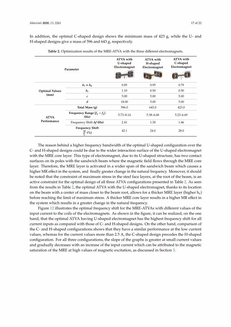
Table 2 shows the optimization results for different configurations of the proposed MRE-ATVA

with a combination of the GA and SQP methods. The optimal values of the design variables are

reported on the top part of the table which are used to calculate the corresponding performance of

the optimal MRE-ATVAs provided at the bottom of the table. The results suggest that the optimal

MRE-ATVA with U-shaped electromagnet presents a 42.1% frequency increase, whereas the C- and

H-shaped types show a 28% and 24% increase in the frequency, respectively. Therefore, the ATVA

having a U-shaped electromagnet shows the maximum frequency range as compared with the other

design configurations where the natural frequency of the absorber could vary from 5.73 to 8.14 Hz.

In addition, the optimal C-shaped design shows the minimum mass of 423 g, while the U- and H-

shaped designs give a mass of 596 and 643 g, respectively.

The reason behind a higher frequency bandwidth of the optimal U-shaped configuration over

the C- and H-shaped designs could be due to the wider interaction surface of the U-shaped

electromagnet with the MRE core layer. This type of electromagnet, due to its U-shaped structure,

has two contact surfaces on its poles with the sandwich beam where the magnetic field flows through

the MRE core layer. Therefore, the MRE layer is activated in a wider span of the sandwich beam

which causes a higher MR effect in the system, and finally greater change in the natural frequency.

Moreover, it should be noted that the constraint of maximum stress in the steel face layers, at the root

of the beam, is an active constraint for the optimal design of all three ATVA configurations presented

in Table 2. As seen from the results in Table 2, the optimal ATVA with the U-shaped electromagnet,

thanks to its location on the beam with a center of mass closer to the beam root, allows for a thicker

MRE layer (higher hc) before reaching the limit of maximum stress. A thicker MRE core layer results

in a higher MR effect in the system which results in a greater change in the natural frequency.

Figure 11. Performance of the sequential quadratic programming (SQP) method when starting fromdifferent initial points.

Executing GA, which uses random population of points, resulted in optimum solutions whichwere close to the global optimum solution. However, once different optimum solutions from the GAwere used as initial points for the SQP algorithm, a unique global optimum solution was obtained.

Table 2 shows the optimization results for different configurations of the proposed MRE-ATVAwith a combination of the GA and SQP methods. The optimal values of the design variables arereported on the top part of the table which are used to calculate the corresponding performance ofthe optimal MRE-ATVAs provided at the bottom of the table. The results suggest that the optimalMRE-ATVA with U-shaped electromagnet presents a 42.1% frequency increase, whereas the C- andH-shaped types show a 28% and 24% increase in the frequency, respectively. Therefore, the ATVAhaving a U-shaped electromagnet shows the maximum frequency range as compared with the otherdesign configurations where the natural frequency of the absorber could vary from 5.73 to 8.14 Hz.

Materials 2020, 13, 2261 17 of 22

In addition, the optimal C-shaped design shows the minimum mass of 423 g, while the U- andH-shaped designs give a mass of 596 and 643 g, respectively.

Table 2. Optimization results of the MRE-ATVA with the three different electromagnets.

Parameter

ATVA withU-shaped

Electromagnet



Parameter

Op

timal

Valu

es

(mm

)

𝒉𝒕 = 𝒉𝒃 0.85 0.95 0.79

𝒉𝐜 1.10 0.50 0.50

𝒄 5.00 5.00 5.00

𝒅 18.00 5.00 5.00

AT

VA

Perfo

rman

ce

Total Mass (g) 596.0 643.0 423.0

Frequency Range [𝒇𝟏−𝒇𝟐]

(Hz) 5.73–8.14 5.38–6.68 5.23–6.69

Frequency Shift 𝜟𝒇 (Hz) 2.41 1.30 1.46

Frequency Shift 𝜟𝒇

𝒇𝟏(%)

42.1 24.0 28.0

Figure 12 illustrates the optimal frequency shift for the MRE-ATVAs with different values of the

input current to the coils of the electromagnets. As shown in the figure, it can be realized, on the one

hand, that the optimal ATVA having U-shaped electromagnet has the highest frequency shift for all

current inputs as compared with those of C- and H-shaped designs. On the other hand, comparison

of the C- and H-shaped configurations shows that they have a similar performance at the low current

values, whereas for the current values more than 2.5 A, the C-shaped design precedes the H-shaped

configuration. For all three configurations, the slope of the graphs is greater at small current values

and gradually decreases with an increase of the input current which can be attributed to the magnetic

saturation of the MRE at high values of magnetic excitation, as discussed in Section 3.

ATVA withH-shaped

Electromagnet



Parameter

Op

timal

Valu

es

(mm

)

𝒉𝒕 = 𝒉𝒃 0.85 0.95 0.79

𝒉𝐜 1.10 0.50 0.50

𝒄 5.00 5.00 5.00

𝒅 18.00 5.00 5.00

AT

VA

Perfo

rman

ce

Total Mass (g) 596.0 643.0 423.0


(Hz) 5.73–8.14 5.38–6.68 5.23–6.69



𝒇𝟏(%)

42.1 24.0 28.0










ATVA withC-shaped

Electromagnet



Parameter

Op

timal

Valu

es

(mm

)

𝒉𝒕 = 𝒉𝒃 0.85 0.95 0.79

𝒉𝐜 1.10 0.50 0.50

𝒄 5.00 5.00 5.00

𝒅 18.00 5.00 5.00

AT

VA

Perfo

rman

ce

Total Mass (g) 596.0 643.0 423.0


(Hz) 5.73–8.14 5.38–6.68 5.23–6.69



𝒇𝟏(%)

42.1 24.0 28.0










Optimal Values(mm)

ht = hb 0.85 0.95 0.79

hc 1.10 0.50 0.50

c 5.00 5.00 5.00

d 18.00 5.00 5.00

ATVAPerformance

Total Mass (g) 596.0 643.0 423.0

Frequency Range [f1 − f2](Hz) 5.73–8.14 5.38–6.68 5.23–6.69

Frequency Shift ∆f (Hz) 2.41 1.30 1.46

Frequency Shift∆ff1

(%)42.1 24.0 28.0

The reason behind a higher frequency bandwidth of the optimal U-shaped configuration over theC- and H-shaped designs could be due to the wider interaction surface of the U-shaped electromagnetwith the MRE core layer. This type of electromagnet, due to its U-shaped structure, has two contactsurfaces on its poles with the sandwich beam where the magnetic field flows through the MRE corelayer. Therefore, the MRE layer is activated in a wider span of the sandwich beam which causes ahigher MR effect in the system, and finally greater change in the natural frequency. Moreover, it shouldbe noted that the constraint of maximum stress in the steel face layers, at the root of the beam, is anactive constraint for the optimal design of all three ATVA configurations presented in Table 2. As seenfrom the results in Table 2, the optimal ATVA with the U-shaped electromagnet, thanks to its locationon the beam with a center of mass closer to the beam root, allows for a thicker MRE layer (higher hc)before reaching the limit of maximum stress. A thicker MRE core layer results in a higher MR effect inthe system which results in a greater change in the natural frequency.

Figure 12 illustrates the optimal frequency shift for the MRE-ATVAs with different values of theinput current to the coils of the electromagnets. As shown in the figure, it can be realized, on the onehand, that the optimal ATVA having U-shaped electromagnet has the highest frequency shift for allcurrent inputs as compared with those of C- and H-shaped designs. On the other hand, comparison ofthe C- and H-shaped configurations shows that they have a similar performance at the low currentvalues, whereas for the current values more than 2.5 A, the C-shaped design precedes the H-shapedconfiguration. For all three configurations, the slope of the graphs is greater at small current valuesand gradually decreases with an increase of the input current which can be attributed to the magneticsaturation of the MRE at high values of magnetic excitation, as discussed in Section 3.

Materials 2020, 13, 2261 18 of 22


Figure 12. Frequency shift versus input current for the three optimal MRE-ATVAs.

8. Conclusions

In this study, a comprehensive design optimization process for a novel MRE-based adaptive

tuned vibration absorber (MRE-ATVA) is investigated. The proposed MRE-ATVA consists of a three-

layer sandwich beam with MRE in the core layer and two electromagnets placed on both ends of the

beam to provide the required magnetic field and to serve as the active mass of the absorbers. Three

potential designs for the electromagnets are investigated in the optimization problem including

electromagnets with U-, H-, and C-shaped designs. A finite element (FE) model of the sandwich beam

is presented and validated with the analytical solution from the literature. Magnetic analysis of the

electromagnets is performed using a developed formulation based on the Ampere’s circuital law and

Gauss’s law. The results of the magnetic analysis of the electromagnets are validated with the

simulation results using a FE magnetic analysis. By combining the FE model of the sandwich beam

and the magnetic model of the electromagnets, a high-fidelity model of the proposed MRE-ATVAs

is constructed, which is subsequently employed to calculate the natural frequency of the complete

absorber device and constraint functions.

A multidisciplinary design optimization problem is finally formulated to identify the optimal

values of the considered geometric structural and magnetic design parameters to maximize the

frequency range of the proposed MRE-ATVA. A combined GA and SQP algorithm was used to find

accurate global optimal solutions of the proposed MRE-ATVAs with three different electromagnet

configurations. The results suggest that the optimal MRE-ATVA with U-shaped electromagnet can

provide the highest frequency shift (42%) in the range of 5.73 to 8.14 Hz. The C- and H-shaped

configurations present a 28% and 24% increase in the natural frequency, respectively. The optimal

adaptive tuned vibration absorbers are all lightweight as their mass is below 700 g. In addition, the

performance of the optimized MRE-ATVA at different input currents is investigated. The results

show that the optimal MRE-ATVA with a U-shaped electromagnet provides the highest frequency

shift irrespective of the applied current. Such optimized lightweight MRE-ATVAs with significant

frequency shift in the low frequency range paves the way for realization of the compact practical

adaptive vibration absorbers that are very effective and reliable for vibration and noise control

applications.

Author Contributions: Conceptualization, M.A.K. and R.S.; methodology, M.A.K., R.S.; modelling and

validation, M.A.K.; resources, M.A.K., R.S. and M.H.; data curation, M.A.K. and M.H.; writing—original draft

preparation, M.A.K.; writing—review and editing, R.S. and M.A.K. and M.H.; supervision, R.S.; project

administration, R.S.; funding acquisition, R.S. All authors have read and agreed to the published version of the

manuscript.

Funding: This research was funded by NSERC, grant no.: RGPIN/6696-2016.

Figure 12. Frequency shift versus input current for the three optimal MRE-ATVAs.

8. Conclusions

In this study, a comprehensive design optimization process for a novel MRE-based adaptive tunedvibration absorber (MRE-ATVA) is investigated. The proposed MRE-ATVA consists of a three-layersandwich beam with MRE in the core layer and two electromagnets placed on both ends of the beamto provide the required magnetic field and to serve as the active mass of the absorbers. Three potentialdesigns for the electromagnets are investigated in the optimization problem including electromagnetswith U-, H-, and C-shaped designs. A finite element (FE) model of the sandwich beam is presentedand validated with the analytical solution from the literature. Magnetic analysis of the electromagnetsis performed using a developed formulation based on the Ampere’s circuital law and Gauss’s law.The results of the magnetic analysis of the electromagnets are validated with the simulation resultsusing a FE magnetic analysis. By combining the FE model of the sandwich beam and the magneticmodel of the electromagnets, a high-fidelity model of the proposed MRE-ATVAs is constructed, whichis subsequently employed to calculate the natural frequency of the complete absorber device andconstraint functions.

A multidisciplinary design optimization problem is finally formulated to identify the optimalvalues of the considered geometric structural and magnetic design parameters to maximize thefrequency range of the proposed MRE-ATVA. A combined GA and SQP algorithm was used to findaccurate global optimal solutions of the proposed MRE-ATVAs with three different electromagnetconfigurations. The results suggest that the optimal MRE-ATVA with U-shaped electromagnet canprovide the highest frequency shift (42%) in the range of 5.73 to 8.14 Hz. The C- and H-shapedconfigurations present a 28% and 24% increase in the natural frequency, respectively. The optimaladaptive tuned vibration absorbers are all lightweight as their mass is below 700 g. In addition,the performance of the optimized MRE-ATVA at different input currents is investigated. The resultsshow that the optimal MRE-ATVA with a U-shaped electromagnet provides the highest frequency shiftirrespective of the applied current. Such optimized lightweight MRE-ATVAs with significant frequencyshift in the low frequency range paves the way for realization of the compact practical adaptivevibration absorbers that are very effective and reliable for vibration and noise control applications.

Author Contributions: Conceptualization, M.A.K. and R.S.; methodology, M.A.K., R.S.; modelling and validation,M.A.K.; resources, M.A.K., R.S. and M.H.; data curation, M.A.K. and M.H.; writing—original draft preparation,M.A.K.; writing—review and editing, R.S. and M.A.K. and M.H.; supervision, R.S.; project administration, R.S.;funding acquisition, R.S. All authors have read and agreed to the published version of the manuscript.

Funding: This research was funded by NSERC, grant no.: RGPIN/6696-2016.

Acknowledgments: Support from the Natural Sciences and Engineering Research Council of Canada (NSERC) isgratefully acknowledged.

Materials 2020, 13, 2261 19 of 22

Conflicts of Interest: The authors declare no conflict of interest.

Appendix A

In this appendix, required formulation for magnetic analysis of the C- and U-shapedelectromagnets is provided, similarly, to the equations developed for the H-shaped electromagnetin Section 5. Parameters have the same meaning as in the case of H-shaped electromagnet unlessotherwise mentioned.

For the C-shaped electromagnet, according to Figure 2b that shows the C-shaped electromagnet,since there is only one closed loop in the path of magnetic flux without any node, the amount of flux isconstant around the loop. In addition, Equation (31) could be written for the C-shaped electromagnetin the following format:

Nc1I + Nc2I + Nc3I = Hcorelcore + Hgaplgap (A1)

The number of turns of wire in the coils of the electromagnet can be estimated as:

Nc1 = Nc2 = cd2D2

Nc3 =d(2c+g)

2D2

(A2)

In addition, the total mass of the electromagnet can be formulated as:

Mel =π4

D2Lwρw + Vscρsc (A3)

where Lw and Vsc could be found with the following relations:

Lw =2cdD2

(t + t + d) +d(2c + g)

D2(t + t + d) (A4)

Vsc = t((2t + d)(2t + 2c + g) − d(2c + g) − gt) (A5)

Similar to what was presented for the H-shaped electromagnet in Figure 10, here, the FE magneticanalysis for the C-shaped electromagnet, performed by the FEMM software, is demonstrated inFigure A1. The input current to the coil is set at 5 A. The considered C-shaped electromagnet hasdimensions of c = d = t =2 cm and a gap of g = 0.5 cm.

Results of magnetic flux density at the center of the gap has also been calculated using bothanalytical model (Equations (A1) to (A5)) and FE analysis (with FEMM software) for different appliedcurrents. Table A1 shows the comparison of the results for the C-shaped electromagnet.

Table A1. Comparison of flux density values at the center of the air gap of the C-shaped electromagnetobtained by analytical magnetic circuit model (Equations (A1) to (A5)) and FE model.


Analytical Magnetic Circuit ModelEquations (A1) to (A5)

Flux Density (mT)FE Analysis Error%

2.5 394 400 1.503 474 480 1.25

3.5 554 560 1.074 635 645 1.55

4.5 716 726 1.385 798 806 0.99

Materials 2020, 13, 2261 20 of 22


Acknowledgments: Support from the Natural Sciences and Engineering Research Council of Canada (NSERC)

is gratefully acknowledged.

Conflicts of Interest: The authors declare no conflict of interest.

Appendix

In this appendix, required formulation for magnetic analysis of the C- and U-shaped

electromagnets is provided, similarly, to the equations developed for the H-shaped electromagnet in

Section 5. Parameters have the same meaning as in the case of H-shaped electromagnet unless

otherwise mentioned.

For the C-shaped electromagnet, according to Figure 2b that shows the C-shaped electromagnet,

since there is only one closed loop in the path of magnetic flux without any node, the amount of flux

is constant around the loop. In addition, Equation (31) could be written for the C-shaped

electromagnet in the following format:

𝑁𝑐1𝐼 + 𝑁𝑐2𝐼 + 𝑁𝑐3𝐼 = 𝐻𝑐𝑜𝑟𝑒𝑙𝑐𝑜𝑟𝑒 + 𝐻𝑔𝑎𝑝𝑙𝑔𝑎𝑝 (A1)

The number of turns of wire in the coils of the electromagnet can be estimated as:

𝑁𝑐1 = 𝑁𝑐2 = 𝑐𝑑

2𝐷2

𝑁𝑐3 = 𝑑(2𝑐 + 𝑔)

2𝐷2 (A2)

In addition, the total mass of the electromagnet can be formulated as:

𝑀𝑒𝑙 = 𝜋

4𝐷2𝐿𝑤𝜌𝑤 + 𝑉𝑠𝑐𝜌𝑠𝑐 (A3)

where 𝐿𝑤 and 𝑉𝑠𝑐 could be found with the following relations:

𝐿𝑤 = 2𝑐𝑑

𝐷2(𝑡 + 𝑡 + 𝑑) +

𝑑(2𝑐 + 𝑔)

𝐷2(𝑡 + 𝑡 + 𝑑) (A4)

𝑉𝑠𝑐 = 𝑡((2𝑡 + 𝑑)(2𝑡 + 2𝑐 + 𝑔) − 𝑑(2𝑐 + 𝑔) − 𝑔𝑡) (A5)

Similar to what was presented for the H-shaped electromagnet in Figure 10, here, the FE

magnetic analysis for the C-shaped electromagnet, performed by the FEMM software, is

demonstrated in Figure A1. The input current to the coil is set at 5 A. The considered C-shaped

electromagnet has dimensions of 𝑐 = 𝑑 = 𝑡 = 2 cm and a gap of 𝑔 = 0.5 cm.

Figure A1. Magnetic flux distribution for the C-shaped electromagnet using FEMM software. Figure A1. Magnetic flux distribution for the C-shaped electromagnet using FEMM software.

For the U-shaped design, considering the U-shaped electromagnet as in Figure 2c, the analyticalmagnetic model can be presented with the following equations:

Nc1I + Nc2I + Nc3I + Nc4I = Hcorelcore + Hgaplgap (A6)

The number of turns of wire in the coils of the electromagnet can be found as:

Nc1 = Nc2 = Nc3 = Nc4 =cd

2D2 (A7)

Moreover, the total mass of the electromagnet can be formulated as:

Mel =π4

D2Lwρw + Vscρsc (A8)

where length of wire Lw and volume of the steel core Vsc could be found with the following relations:

Lw =4cdD2

(t + t + d) (A9)

Vsc = 2t((2t + d)(c + t) − cd) (A10)

Figure A2 shows the FE magnetic analysis for the U-shaped electromagnet, performed by theFEMM software when the input current to the coil is set at 5 A.

Materials 2020, 13, 2261 21 of 22


Results of magnetic flux density at the center of the gap has also been calculated using both

analytical model (Equations (A1) to (A5)) and FE analysis (with FEMM software) for different applied

currents. Table A1 shows the comparison of the results for the C-shaped electromagnet.

Table A1. Comparison of flux density values at the center of the air gap of the C-shaped electromagnet

obtained by analytical magnetic circuit model (Equations (A1) to (A5)) and FE model.

Input Current (A)

Flux Density (mT)

Analytical Magnetic Circuit Model

Equations (A1) to (A5)

Flux Density (mT)

FE Analysis Error%

2.5 394 400 1.50

3 474 480 1.25

3.5 554 560 1.07

4 635 645 1.55

4.5 716 726 1.38

5 798 806 0.99

For the U-shaped design, considering the U-shaped electromagnet as in Figure 2c, the analytical

magnetic model can be presented with the following equations: 𝑁𝑐1𝐼 + 𝑁𝑐2𝐼 + 𝑁𝑐3𝐼 + 𝑁𝑐4𝐼 = 𝐻𝑐𝑜𝑟𝑒𝑙𝑐𝑜𝑟𝑒 + 𝐻𝑔𝑎𝑝𝑙𝑔𝑎𝑝 (A6)

The number of turns of wire in the coils of the electromagnet can be found as:

𝑁𝑐1 = 𝑁𝑐2 = 𝑁𝑐3 = 𝑁𝑐4 = 𝑐𝑑

2𝐷2 (A7)

Moreover, the total mass of the electromagnet can be formulated as:

𝑀𝑒𝑙 = 𝜋

4𝐷2𝐿𝑤𝜌𝑤 + 𝑉𝑠𝑐𝜌𝑠𝑐 (A8)

where length of wire 𝐿𝑤 and volume of the steel core 𝑉𝑠𝑐 could be found with the following

relations:

𝐿𝑤 = 4𝑐𝑑

𝐷2(𝑡 + 𝑡 + 𝑑) (A9)

𝑉𝑠𝑐 = 2𝑡((2𝑡 + 𝑑)(𝑐 + 𝑡) − 𝑐𝑑) (A10)

Figure A2 shows the FE magnetic analysis for the U-shaped electromagnet, performed by the

FEMM software when the input current to the coil is set at 5 A.

Figure A2. Magnetic flux distribution for the U-shaped electromagnet using FEMM software. Figure A2. Magnetic flux distribution for the U-shaped electromagnet using FEMM software.

In addition, the results of magnetic flux density at the center of the gap calculated by utilizingboth analytical model (using Equations (A6) to (A10)) and FE analysis (with FEMM software) fordifferent input currents are shown in Table A2 for the U-shaped electromagnet.

Table A2. Comparison of the flux density values at the center of the air gap of the U-shapedelectromagnet obtained by analytical magnetic circuit model (Equations (A6) to (A10)) and FE model.


Analytical Magnetic Circuit ModelEquations (A6) to (A10)

Flux Density (mT)FE Analysis Error%

2.5 189 190 0.533 226 228 0.88

3.5 264 266 0.754 302 304 0.66

4.5 339 341 0.595 377 379 0.53

References

1. Asadi Khanouki, M.; Sedaghati, R.; Hemmatian, M. Experimental characterization and microscale modelingof isotropic and anisotropic magnetorheological elastomers. Compos. Part B Eng. 2019, 176, 107311. [CrossRef]

2. Bellelli, A.; Spaggiari, A. Magneto-mechanical characterization of magnetorheological elastomers. J. Intell.Mater. Syst. Struct. 2019, 30, 2534–2543. [CrossRef]

3. Samal, S.; Kolinova, M.; Blanco, I. The Magneto-Mechanical Behavior of Active Components in Iron-ElastomerComposite. J. Compos. Sci. 2018, 2, 54. [CrossRef]

4. Eem, S.-H.; Koo, J.-H.; Jung, H.-J. Feasibility study of an adaptive mount system based on magnetorheologicalelastomer using real-time hybrid simulation. J. Intell. Mater. Syst. Struct. 2019, 30, 701–707. [CrossRef]

5. Lerner, A.A.; Cunefare, K.A. Performance of MRE-based vibration absorbers. J. Intell. Mater. Syst. Struct.2008, 19, 551–563. [CrossRef]

6. Sun, S.; Chen, Y.; Yang, J.; Tian, T.; Deng, H.; Li, W.; Du, H.; Alici, G. The development of an adaptive tunedmagnetorheological elastomer absorber working in squeeze mode. Smart Mater. Struct. 2014, 23, 075009.[CrossRef]

http://dx.doi.org/10.1016/j.compositesb.2019.107311

http://dx.doi.org/10.1177/1045389X19828828

http://dx.doi.org/10.3390/jcs2030054

http://dx.doi.org/10.1177/1045389X18754347

http://dx.doi.org/10.1177/1045389X07077850

http://dx.doi.org/10.1088/0964-1726/23/7/075009

Materials 2020, 13, 2261 22 of 22

7. Sun, S.; Deng, H.; Yang, J.; Li, W.; Du, H.; Alici, G. Performance evaluation and comparison ofmagnetorheological elastomer absorbers working in shear and squeeze modes. J. Intell. Mater. Syst.Struct. 2015, 26, 1757–1763. [CrossRef]

8. Yang, C.; Fu, J.; Yu, M.; Zheng, X.; Ju, B. A new magnetorheological elastomer isolator in shear–compressionmixed mode. J. Intell. Mater. Syst. Struct. 2015, 26, 1290–1300. [CrossRef]

9. Xin, F.-L.; Bai, X.-X.; Qian, L.-J. Principle, modeling, and control of a magnetorheological elastomer dynamicvibration absorber for powertrain mount systems of automobiles. J. Intell. Mater. Syst. Struct. 2016, 28,2239–2254. [CrossRef]

10. Parlak, Z.; Engin, T.; Çallı, I. Optimal design of MR damper via finite element analyses of fluid dynamic andmagnetic field. Mechatronics 2012, 22, 890–903. [CrossRef]

11. Nguyen, Q.-H.; Choi, S.-B. Optimal design of a vehicle magnetorheological damper considering the dampingforce and dynamic range. Smart Mater. Struct. 2008, 18, 015013. [CrossRef]

12. Imaduddin, F.; Mazlan, S.A.; Zamzuri, H. A design and modelling review of rotary magnetorheologicaldamper. Mater. Des. 2013, 51, 575–591. [CrossRef]

13. Elliott, C.M.; Buckner, G.D. Design optimization of a novel elastomeric baffle magnetorheological fluiddevice. J. Intell. Mater. Syst. Struct. 2018, 29, 3774–3791. [CrossRef]

14. Dong, Z.; Feng, Z.; Chen, Y.; Yu, K.; Zhang, G. Design and Multiobjective Optimization of MagnetorheologicalDamper considering the Consistency of Magnetic Flux Density. Shock Vib. 2020, 2020. [CrossRef]

15. Hirunyapruk, C.; Brennan, M.; Mace, B.; Li, W. A tunable magneto-rheological fluid-filled beam-like vibrationabsorber. Smart Mater. Struct. 2010, 19, 055020. [CrossRef]

16. Lord Magnetorheological (MR) Store, Data Sheet for MRF-132DG Magnetorheological Fluid. Availableonline: http://www.lordmrstore.com/lord-mr-products/mrf-132dg-magneto-rheological-fluid (accessed on20 April 2020).

17. Nguyen, P.-B.; Choi, S.-B. A new approach to magnetic circuit analysis and its application to the optimaldesign of a bi-directional magnetorheological brake. Smart Mater. Struct. 2011, 20, 125003. [CrossRef]

18. ASTM International. Standard Specification for Standard Nominal Diameters and Cross-Sectional Areas of AWGSizes of Solid Round Wires Used as Electrical Conductors; ASTM International: West Conshohocken, PA, USA,2018; ASTM B258-18.

19. Grewal, J.S.; Sedaghati, R.; Esmailzadeh, E. Vibration analysis and design optimization of sandwich beamswith constrained viscoelastic core layer. J. Sandw. Struct. Mater. 2013, 15, 203–228. [CrossRef]

20. Nayak, B.; Dwivedy, S.K.; Murthy, K. Vibration analysis of a three-layer magnetorheological elastomerembedded sandwich beam with conductive skins using finite element method. Proc. Inst. Mech. Eng. Part CJ. Mech. Eng. Sci. 2013, 227, 714–729. [CrossRef]

21. Eshaghi, M.; Rakheja, S.; Sedaghati, R. An accurate technique for pre-yield characterization of MR fluids.Smart Mater. Struct. 2015, 24, 065018. [CrossRef]

22. Mead, D.; Markus, S. Loss factors and resonant frequencies of encastre damped sandwich beams. J. SoundVib. 1970, 12, 99–112. [CrossRef]

23. Sudhoff, S.D. Power Magnetic Devices: A Multi-Objective Design Approach; John Wiley & Sons: Hoboken, NJ,USA, 2014.

© 2020 by the authors. Licensee MDPI, Basel, Switzerland. This article is an open accessarticle distributed under the terms and conditions of the Creative Commons Attribution(CC BY) license (http://creativecommons.org/licenses/by/4.0/).

http://dx.doi.org/10.1177/1045389X14568819

http://dx.doi.org/10.1177/1045389X14541492

http://dx.doi.org/10.1177/1045389X16672731

http://dx.doi.org/10.1016/j.mechatronics.2012.05.007

http://dx.doi.org/10.1088/0964-1726/18/1/015013

http://dx.doi.org/10.1016/j.matdes.2013.04.042

http://dx.doi.org/10.1177/1045389X18799211

http://dx.doi.org/10.1155/2020/7050356

http://dx.doi.org/10.1088/0964-1726/19/5/055020

http://www.lordmrstore.com/lord-mr-products/mrf-132dg-magneto-rheological-fluid

http://dx.doi.org/10.1088/0964-1726/20/12/125003

http://dx.doi.org/10.1177/1099636213476510

http://dx.doi.org/10.1177/0954406212451812

http://dx.doi.org/10.1088/0964-1726/24/6/065018

http://dx.doi.org/10.1016/0022-460X(70)90050-7

http://creativecommons.org/

http://creativecommons.org/licenses/by/4.0/.

Documents

Multidisciplinary Design Optimization of a Novel Sandwich