Embed Size (px)
Citation preview

MULTIDISCIPLINARY AIRCRAFT DESIGN AND OPTIMISATION USING A ROBUST EVOLUTIONARY TECHNIQUE WITH VARIABLE FIDELITY MODELS
The University of SydneyL. F. GonzalezE. J. WhitneyK. Srinivas
Pole ScientifiqueJ. Périaux
10th AIAA/ISSMO Multidisciplinary Analysis and Optimization Conference, Albany, New York,USA, 30 Aug - 1 Sep 2004,

Outline• Introduction
– Problems in aeronautical design and optimisation– The need for Evolutionary algorithms
• Theory– Evolution Algorithms (EAs).– Multidisciplinary –Multi-objective Design – Hierarchical Asynchronous Evolutionary Algorithm (HAPEA).
• Application- Mathematical Test functions- Two real world examples
• Conclusions

Multidisciplinary aircraft design and optimisation
• Aircraft Deign is multidisciplinary in nature and there is a strong interaction between the different multi-physics involved (aerodynamics , structures , propulsion)
• A tradeoff between aerodynamic performance and other objectives becomes necessary.

• Multidisciplinary design problems involve search space that are multi-modal, non-convex or discontinuous.
• Traditional methods use deterministic approach and rely heavily on the use of iterative trade-off studies between conflicting requirements.
Problems in Aerodynamic Optimisation (1)

• Traditional optimisation methods will fail to find the real answer in many real engineering applications, (Noise, complex functions).
Problems in Aerodynamic Optimisation (2)
•Question- High Fidelity model? Or a thorough search with a Low Fidelity Model?
•Commercial solvers are essentially inaccessible from a modification point of view (they are black-boxes).

Why Evolution?
• Evolution Algorithms can explore large variations in designs.
• Robust towards noise and local minima and easy to to parallelise, reducing computation time.
• Provide optimal solutions for single and multi-objective problems or calculating a robust Nash game
• EAs successively map multiple populations of points, allowing solution diversity.

Evolution Algorithms
What are EAs.
• Computers can be adapted to perform this evolution process.
Crossover Mutation
Fittest
Evolution• Based on the Darwinian theory of evolution Populations of individuals evolve and reproduce by means of mutation and crossover operators and compete in a set environment for survival of the fittest.
Introduction to Multi-Objective Optimisation (1)• Aeronautical design problems normally require a
simultaneous optimisation of conflicting objectives and associated number of constraints. They occur when two or more objectives that cannot be combined rationally. For example:
• Drag at two different values of lift.
• Drag and thickness.
• Pitching moment and maximum lift.
• Best to let the designer choose after the optimisation phase.

Maximise/ Minimise
Subjected to constraints
• objective functions, output (e.g. cruise efficiency).
• x: vector of design variables, inputs (e.g. aircraft geometry ) with upper and lower bounds;
• g(x) equality constraints and h(x) inequality constraints: (e.g. element von Mises stresses); in general these are nonlinear functions of the design variables.
Nixf ...11
Kkxh
Njxg
k
i
...10
...10
xfi
Introduction to Multi-Objective Optimisation (2)

• A set of solutions that are non-dominated w.r.t all others points in the search space, or that they dominate every other solution in the search space except fellow members of the Pareto optimal set.
Pareto Optimal Set

Our Approach:
• Parallel Computing and Asynchronous Evaluation
• Pareto Tournament Selection
• Hierarchical Population Topology
Hierarchical Asynchronous Parallel Evolutionary Algorithms (HAPEA)

Evolution AlgorithmAsynchronous
Evaluator
1 individual
1 individual
Different Speeds
Parallel Computing and Asynchronous Evaluation

Asynchronous Evaluation
Suspend the idea of generation
Solution can be generated in and out of order
Processors – Can be of different speeds Added at random
Any number of them possible
Methods of solutions to MO and MDO -> variable time to complete.
Time to solve non-linear PDE - > Depends upon geometry
Why asynchronous
How:

Asynchronous Evaluation
Methods of solutions to MO and MDO -> variable time to complete.
Time TO SOLVE NON-linear pfF - > DEPENDS UPON GEOMETRY
Traditional EAs -> create an unnecessary bottleneck when used on parallel
computers;
-> i.e processors that have already completed their solutions will remain idle until all processors have completed their work.

• The selection operator is a novel approach to determine whether an individual x is to be accepted into the main population
• Create a tournament
Where B is the selection buffer.
1 2
1 1, ,... ;
6 2nQ q q q B B n B
Population
Tournament Q
Asynchronous Buffer
Evaluate x
If x not dominated
x
Pareto Tournament Selection

Hierarchical Population Topology
Model 1precise model
Model 2intermediate
model
Model 3approximate model
Exploration(large mutation span)
Exploitation(small
mutation span)
• Ackley
• MOEAs Examples
Optimisation of Analytical Test Functions

Test Functions: Ackley
2
1 1
1 10.2 cos(2
N N
i ii i
x xN Nf N e Ne e
Increasing number of variables

• Here our EA solves a two objective problem with two design variables. There are two possible Pareto optimal fronts; one obvious and concave, the other deceptive and convex
MOEA Examples

MOEA Examples
• Again, we solve a two objective problem with two design variables however now the optimal Pareto front contains four discontinuous regions
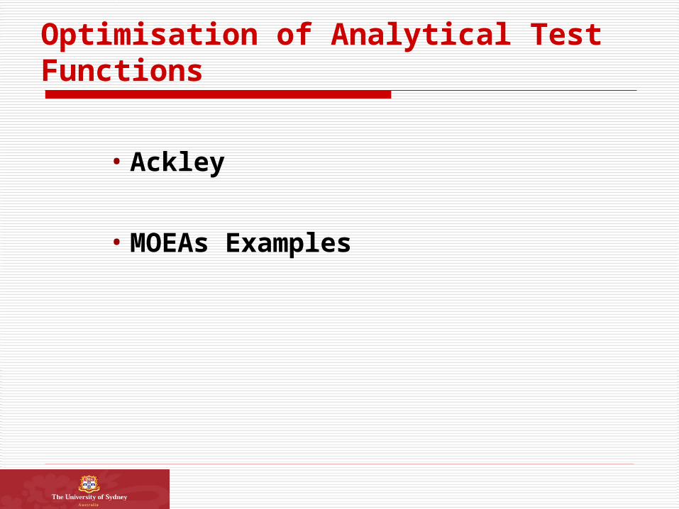
Results So Far…
Evaluations CPU Time
Traditional 2311 224 152m20m
New Technique
504 490(-78%)
48m 24m(-68%)
• The new technique is approximately three times faster than other similar EA methods.
• We have successfully coupled the optimisation code to different compressible and incompressible CFD codes and also to some aircraft design codes
CFD Aircraft Design HDASS MSES XFOIL Flight Optimisation
Software (FLOPS) FLO22 Nsc2ke ADS (In house)
• A testbench for single and multiobjective problems has been developed and tested

Applications So Far… (1)
• Constrained aerofoil design for transonic transport aircraft 3% Drag reduction
• UAV aerofoil design-Drag minimisation for high-speed
transit and loiter conditions. -Drag minimisation for high-speed
transit and takeoff conditions.
• Exhaust nozzle design for minimum losses.

Applications So Far… (2)
• Three element aerofoil reconstruction from surface pressure data.
• UCAV MDO Whole aircraft multidisciplinary design. Gross weight minimisation and cruise
efficiency Maximisation. Coupling with NASA code FLOPS
2 % improvement in Takeoff GW and Cruise Efficiency
• AF/A-18 Flutter model validation.

Applications So Far… (3)
• Transonic wing design Two Objectives
• UAV Wing Design
• Wind Tunnel Test :
Evolved AerofoilsEvolved WingsEvolved Aircrafts (in progress)

Two Representative Examples
• Three Element Aerofoil Euler Reconstruction.
• Multidisciplinary UAV Design Optimisation
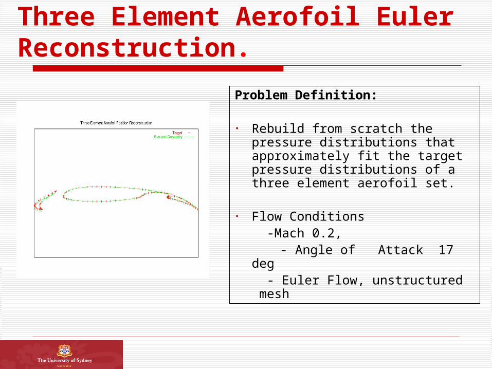
Three Element Aerofoil Euler Reconstruction.
Problem Definition:
• Rebuild from scratch the pressure distributions that approximately fit the target pressure distributions of a three element aerofoil set.
• Flow Conditions -Mach 0.2,
- Angle of Attack 17 deg - Euler Flow, unstructured mesh

Design variables
Fitness Function
The fitness function is the RMS error of the surface
pressure coefficients on all the three elements
Multi-element aerofoil reconstruction problem
,x y The design variables are the position
And rotation of the slat and flap
Upper and lower bounds of position and rotation are and respectively , 0.05x y 30
2
arg1
1min
N
candidate T etelements i
F Cp CpN

Implementation
Population size: 40 Grid nbv 2500
Single Population EA (EA SP)
Hierarchical Asynchronous Parallel EA (HAPEA)
Population size: 40
Population size: 40
Population size: 40
Viscous: Grid nbv 2500
Viscous: Grid nbv 2000
Viscous: Grid nbv 1500

Pressure Distribution

Candidate and Target Geometries

Example of Convergence History.
A better solution in lower computing time

UAV Conceptual DesignOptimisation Problem
Minimise two objectives:
Gross weight min(WG)Endurance min (1/E)
Subject to: Takeoff distance <1000 ft,
Alt Cr > 40000 ROC > 1000 fpm, Endurance > 24 hrs
With respect to:
external geometry of the aircraft
• Mach = 0.3• Endurance > 24
hrs • Cruise Altitude:
40000 ft

Design Variables
In total we have 29 design variables
Design Variable Lower Bound
Upper Bound
Wing Area (sq ft) 280 330
Aspect Ratio S 18 25.2
Wing Sweep (deg)
0.0 8.0
Wing Taper Ratio 0.28 0.8
13 Configuration Design variables
Camber
Twist
Win
g

Design Variables
Camber
Twist
Horizontal Tail Area (sq ft)
65.0 85.0
HT Aspect Ratio 3.0 15.0
HT Taper Ratio 0.2 0.55
HT Sweep (deg) 12.0 15.0
Vertical Tail Area (sq ft)
11.0 29.0
VT Aspect Ratio 1.0 3.2
VT Taper Ratio 0.28 0.62
VT Sweep (deg) 12.0 34.0
Fuselage Diameter
2.6 5.0
Tail
Fuselage
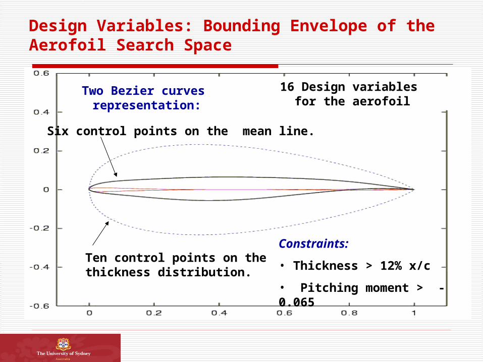
Design Variables: Bounding Envelope of the Aerofoil Search Space
Ten control points on the thickness distribution.
16 Design variables for the aerofoil
Constraints:
• Thickness > 12% x/c
• Pitching moment > -0.065
Two Bezier curves representation:
Six control points on the mean line.

Mission profile

Structural & weight analysis
A compromise on fidelity modelsVortex induced drag: VLMpcViscous drag: frictionAerofoil Design Xfoil
pMOEA (HAPEA)Optimisation
Aircraft designand analysis
Aerodynamics
FLOPS
FLOPS (Modified to accept user computed aerodynamic data)
Design Tools

Implementation
Population size: 20
Population size: 20
Population size: 20
Grid 141x 74x 36 on aerofoil, 20 x 6 on Vortex model
Grid 109x 57x 27 on aerofoil, 17 x 6 on Vortex model
Grid 99x 52x 25 on aerofoil, 15 x 6 on Vortex model

Pareto optimal region
Objective 1 optimal
Objective 2 optimal
Compromise

Sample of Pareto Optimal configurations
Pareto Member 0
Pareto Member 14
Pareto Member 16
Pareto Member 19

• The results indicate that aircraft design optimisation and shape optimisation problem can be resolved with an evolutionary approach using a hierarchical topology.
• The new method contributes to the development of numerical tools required for the complex task of MDO and aircraft design.
• A practical design of a long endurance high altitude UAV was studied and realistic designs were obtained.
• No problem specific knowledge is required The method appears to be broadly applicable to different analysis codes
• A family of Pareto optimal configurations was obtained giving the designer a restricted search space to proceed into more details phases of design.
Conclusions

Acknowledgements
• The authors would like to thank Arnie McCullers at NASA LARC for providing the FLOPS code.
• The authors would like to acknowledge Professor Steve Armfield and Dr Patrick Morgan at The University of Sydney for providing the facilities on using the cluster of computers.
• The authors would like to thank Professor M. Drela for providing the MSES code
• Also to Professor K. Deb for discussions on developments and applications of MOEA during his visit to The University of Sydney in 2003.

Questions…

ADDITIONAL SLIDES

• Flow is treated as two dimensional, inviscid and is calculated using B. Mohammadi code NSC2ke
• The solver uses unstructured mesh which are generated using Bamg.
• The computations stop when the 2-norm of the residual falls below a prescribed limit, in this case
CFD Solver
310

Optimization Methods
• Guess /Intuition: decreases as the increasing dimensionality.
• Nonlinear simplex: simple and robust but inefficient for more than a few design variables.
• Grid or random search: the cost of searching the design space increases rapidly with the number of design variables.
• Gradient-based: it is most efficient for a large number of design variables; assumes the objective function is “well-behaved”.
• Evolution algorithms: good for discrete design variables and very robust; but infeasible when using a large number of design variables.

Evolution AlgorithmAsynchronous
Evaluator
1 individual
1 individual
Different Speeds
• Ignores the concept of generation-based solution.
• Fitness functions are computed asynchronously.
• Only one candidate solution is generated at a time, and only one individual is incorporated at a time rather than an entire population at every generation as is traditional EAs.
• Solutions can be generated and returned out of order.
Asynchronous Evaluation (1)

Evolution AlgorithmAsynchronous
Evaluator
1 individual
1 individual
Different Speeds
• No need for synchronicity no possible wait-time bottleneck.
• No need for the different processors to be of similar speed.
• Processors can be added or deleted dynamically during the execution.
• There is no practical upper limit on the number of processors we can use.
• All desktop computers in an organisation are fair game.
Asynchronous Evaluation (2)

Generation –based approach used by evolutionary algorithm, traditional genetic algorithms and evolution strategy create an unnecessary bottleneck when used on parallel computers , i.e., the processors that have already completed their solutions will remain idle until all processors have completed their work
Need for Asynchronous Evaluation
cases used in engineering today may take different times to complete their operations
Time taken for solutions of non-linear partial differential equations will strongly depend
upon the geometry.

Methods of solutions to MO and MDO -> VARIABLE TIME TO COMPLETE.
Time TO SOLVE NON-linear pfF - > DEPENDS UPON GEOMETRY
Traditional EAs -> create an unnecessary bottleneck when used on parallel computers; -> I.E processors that have already completed their solutions will remain idle until all processors have completed their work.

Why MOEAs:• MOEA have been studied intensively in the last 8 years and show
to be promising and effective for different non -linear problems.• In Multi-objective optimisation we seek to find a set of Pareto
optimal solutions which are better those other solutions in all objectives.
• The two main desirable characteristics a MOEA (DEb 2003) are:
-- Convergence to true Pareto optimal set -- Good Diversity among the solutions on the optimal set
pMOEA • In general “..a pMOEA seeks to find as good or better MOP solutions
in less time than its serial MOEA counterpart, use less resources, and /or search more of the solution space , i.e. , increased efficiency and effectiveness [Veldhuizen et al 2003]
Multi-Objective EAs (MOEAs) and parallel (pEAs)

Traditional EA techniques, hierarchical methods , deterministic and EAs
Navier Stokes computationally expensive but accurate) –panel methods ( fast but could be unstable)
Bezier , Splines, depending on the problem
Parallelization strategy
Optimisation Method
Flow analysis method
Geometry Representation
Implementation
pMOEAs
Components of pEA optimisation

• Solved on a single population• Asynchronous: Assign a small fictitious delay to each
function evaluation. This will vary uniformly between two values fastest and lowest. Evaluate asynchronously.
• Synchronous: Assign the same delay to all
individuals in advance. Wait until the slowest evaluation is completed, as it will occur in practice on a cluster of computers.
• Four unknowns=4), Stopping Condition = 0.0001, 25 runs. Configurations up to tslowest /tfastest = 5
Asynchronous Test Case – Sphere Function

Aircraft Design and Analysis
• The FLOPS (FLight OPtimisation System) solver developed by L. A. (Arnie) McCullers, NASA Langley Research Center was used for evaluating the aircraft configurations.
• FLOPS is a workstation based code with capabilities for conceptual and preliminary design of advanced concepts.
• FLOPS is multidisciplinary in nature and contains several analysis modules including: weights, aerodynamics, engine cycle analysis, propulsion, mission performance, takeoff and landing, noise footprint, cost analysis, and program control.
• FLOPS has capabilities for optimisation but in this case was used only for analysis.
• Drag is computed using Empirical Drag Estimation Technique (EDET) - Different hierarchical models are being adapted for drag build up using higher fidelity models.

Conclusions• The proper use of evolutionary techniques for MDO can reduce weight
and improve endurance of an aircraft concept by minor changes in the design variables.
• The results obtained for the aircraft design optimisation are encouraging and promote application of the method with higher fidelity solvers and approximation techniques.

Evolutionary Design Optimisation
Problem Definition
HAPEA Optimiser Setup
Do While Convergence not reached
Create and evaluate initial population
Generate and evaluate new candidates
Evaluation of Candidates
Compute the flow around the aerofoil sections and obtain a Cdo estimate
for the wing
Create drag polar on the candidate geometry Satisfying trim conditions.
Analyze each configuration using FLOPS)
Compute Objective Functions
Evolve/ modify design variables on optimiser until stopping criteria is met.

Aerodynamic Analysis
Control Points

Sample of Pareto Optimal configurations
Pareto Member 0
Pareto Member 14
Pareto Member 16
Pareto Member 19
AR =23.77
SW = 321.74 ft2
SWEEP = 4.87
TR = 0.48
ARHT = 5.43
SWPWT = 10.74
TRHT = 0.43
FW = 3148 Lbs
ENDR = 1846 min
AR =24.30
SW =321.2 ft2
SWEEP =2.77 deg
TR = 0.45
ARHT = 5.61
SWPWT = 5.79
TRHT = 0.40
FW =3486 Lbs
ENDR= 2184 min
AR = 18.9
SW = 301.2 ft2
SWEEP = 7.07
TR = 0.70
ARHT = 3.43
SWPWT = 3.48
TRHT = 0.33
FW =2978 Lbs
ENDR= 1533 min
AR = 24.14
SW = 305 ft2
SWEEP =2.01 deg
TR = 0.62
ARHT = 4.9
SWPWT = 6.55
TRHT = 0.44
FW =3337 Lbs
ENDR= 2008 min

Convergence history for objective one