Idea League

Joint Master's in Applied Geophysics

Multicomponent Seismic Processing for Coherent Noise Suppression and

Arrival Identification

DAVID SOLLBERGER

MASTER THESIS

TU DELFT

ETH ZÜRICH

RWTH AACHEN

Supervisors: Prof. Dr. Stewart A. Greenhalgh

Dr. Cedric Schmelzbach

Zürich, August 9, 2013

i

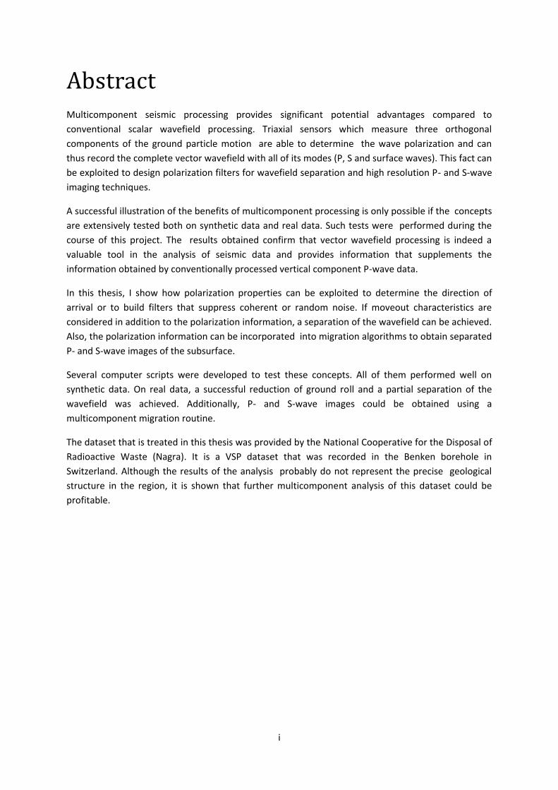
Abstract Multicomponent seismic processing provides significant potential advantages compared to conventional scalar wavefield processing. Triaxial sensors which measure three orthogonal components of the ground particle motion are able to determine the wave polarization and can thus record the complete vector wavefield with all of its modes (P, S and surface waves). This fact can be exploited to design polarization filters for wavefield separation and high resolution P- and S-wave imaging techniques.

A successful illustration of the benefits of multicomponent processing is only possible if the concepts are extensively tested both on synthetic data and real data. Such tests were performed during the course of this project. The results obtained confirm that vector wavefield processing is indeed a valuable tool in the analysis of seismic data and provides information that supplements the information obtained by conventionally processed vertical component P-wave data.

In this thesis, I show how polarization properties can be exploited to determine the direction of arrival or to build filters that suppress coherent or random noise. If moveout characteristics are considered in addition to the polarization information, a separation of the wavefield can be achieved. Also, the polarization information can be incorporated into migration algorithms to obtain separated P- and S-wave images of the subsurface.

Several computer scripts were developed to test these concepts. All of them performed well on synthetic data. On real data, a successful reduction of ground roll and a partial separation of the wavefield was achieved. Additionally, P- and S-wave images could be obtained using a multicomponent migration routine.

The dataset that is treated in this thesis was provided by the National Cooperative for the Disposal of Radioactive Waste (Nagra). It is a VSP dataset that was recorded in the Benken borehole in Switzerland. Although the results of the analysis probably do not represent the precise geological structure in the region, it is shown that further multicomponent analysis of this dataset could be profitable.

ii

Contents Abstract .................................................................................................................................................... i

Contents ................................................................................................................................................... ii

Chapter 1: Introduction........................................................................................................................... 1

1.1. Multicomponent seismic records and their application .............................................................. 1

1.2. Thesis objectives and outline ....................................................................................................... 2

Chapter 2: Single Station Polarization Analysis ....................................................................................... 3

2.1. Seismic direction finding .............................................................................................................. 3

2.1.1. The direction finding problem ............................................................................................... 3

2.1.1.1. Covariance matrix eigendecomposition ......................................................................... 4

2.1.1.2. Vector centroid and upper hemisphere projection ....................................................... 5

2.1.1.3. Brute force power maximization .................................................................................... 7

2.1.1.4. Hodograms, semblance and cross correlation ............................................................. 10

2.1.1.5. Experimental difficulties of single station seismic direction finding ............................ 13

2.2. Single Station Rotation and Polarization Filtering ...................................................................... 15

2.3. Real Data examples .................................................................................................................... 18

2.3.1. Two component rotation .................................................................................................... 18

2.3.2. Surface wave suppression ................................................................................................... 18

Chapter 3: Array Polarization Analysis .................................................................................................. 21

3.1. Theory of the discrete Radon transform .................................................................................... 21

3.1.1. Aliasing in the Radon transform .......................................................................................... 23

3.2. Controlled direction reception filtering (CDR) ........................................................................... 24

3.2.1. CDRI: Radon transform and rotation ................................................................................... 24

3.2.2. CDRII: Polarization gain function ......................................................................................... 26

3.3. Synthetic Data Examples ............................................................................................................ 27

Chapter 4: Multicomponent Migration ................................................................................................. 33

4.1. Multicomponent pre-stack Kirchhoff migration ........................................................................ 33

4.2. Synthetic Data Example .............................................................................................................. 35

Chapter 5: Multicomponent Analysis of a VSP Dataset ........................................................................ 39

5.1. Vertical seismic profiling (VSP) ................................................................................................... 39

5.2. Introduction to the site .............................................................................................................. 39

5.3. Data Processing .......................................................................................................................... 40

5.3.1. Preprocessing ...................................................................................................................... 40

iii

5.3.1.1. Rotation of the horizontal components ....................................................................... 41

5.3.1.2. Bandpass filtering ......................................................................................................... 41

5.3.1.3. Separation into upgoing and downgoing wavefields ................................................... 41

5.3.2. Multicomponent Analysis .................................................................................................... 43

Chapter 6: Conclusions and Outlook ..................................................................................................... 47

6.1. Conclusions ................................................................................................................................. 47

6.2. Outlook ....................................................................................................................................... 48

Bibliography ..................................................................................................................................... 49

List of Figures ........................................................................................................................................ 52

Appendix A ............................................................................................................................................ 55

Appendix B ............................................................................................................................................ 57

Appendix C ............................................................................................................................................ 59

Acknowledgements .............................................................................................................................. 61

iv

1

1Chapter 1

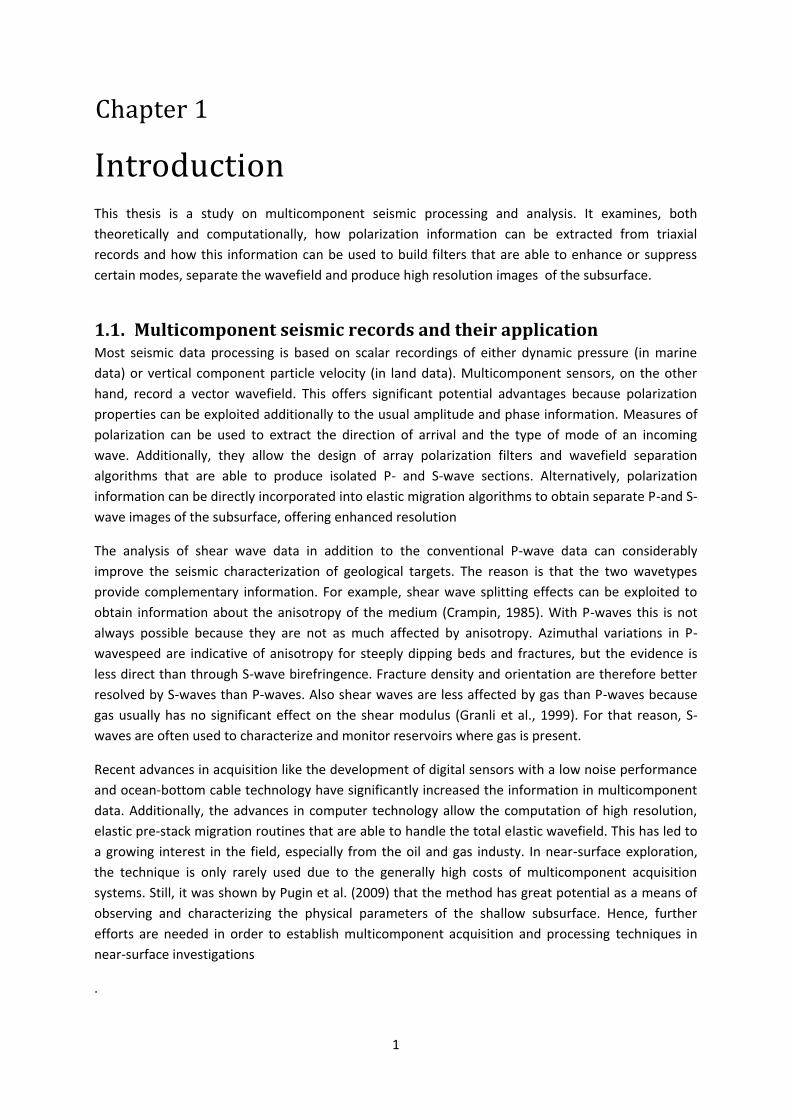
Introduction This thesis is a study on multicomponent seismic processing and analysis. It examines, both theoretically and computationally, how polarization information can be extracted from triaxial records and how this information can be used to build filters that are able to enhance or suppress certain modes, separate the wavefield and produce high resolution images of the subsurface.

1.1. Multicomponent seismic records and their application Most seismic data processing is based on scalar recordings of either dynamic pressure (in marine data) or vertical component particle velocity (in land data). Multicomponent sensors, on the other hand, record a vector wavefield. This offers significant potential advantages because polarization properties can be exploited additionally to the usual amplitude and phase information. Measures of polarization can be used to extract the direction of arrival and the type of mode of an incoming wave. Additionally, they allow the design of array polarization filters and wavefield separation algorithms that are able to produce isolated P- and S-wave sections. Alternatively, polarization information can be directly incorporated into elastic migration algorithms to obtain separate P-and S-wave images of the subsurface, offering enhanced resolution

The analysis of shear wave data in addition to the conventional P-wave data can considerably improve the seismic characterization of geological targets. The reason is that the two wavetypes provide complementary information. For example, shear wave splitting effects can be exploited to obtain information about the anisotropy of the medium (Crampin, 1985). With P-waves this is not always possible because they are not as much affected by anisotropy. Azimuthal variations in P-wavespeed are indicative of anisotropy for steeply dipping beds and fractures, but the evidence is less direct than through S-wave birefringence. Fracture density and orientation are therefore better resolved by S-waves than P-waves. Also shear waves are less affected by gas than P-waves because gas usually has no significant effect on the shear modulus (Granli et al., 1999). For that reason, S-waves are often used to characterize and monitor reservoirs where gas is present.

Recent advances in acquisition like the development of digital sensors with a low noise performance and ocean-bottom cable technology have significantly increased the information in multicomponent data. Additionally, the advances in computer technology allow the computation of high resolution, elastic pre-stack migration routines that are able to handle the total elastic wavefield. This has led to a growing interest in the field, especially from the oil and gas industy. In near-surface exploration, the technique is only rarely used due to the generally high costs of multicomponent acquisition systems. Still, it was shown by Pugin et al. (2009) that the method has great potential as a means of observing and characterizing the physical parameters of the shallow subsurface. Hence, further efforts are needed in order to establish multicomponent acquisition and processing techniques in near-surface investigations

.

2

1.2. Thesis objectives and outline The main objective of this thesis is to theoretically and computationally investigate the potential of multicomponent seismic processing. First, a detailed review of the concepts of polarization analysis- both single station and multi-station, as well as multicomponent migration will be given. The theory will then be illustrated and reinforced by synthetic data examples and finally put to the test on a real dataset. The main goals of the analysis are: the rotation of triaxial or biaxial data into the direction of arrival, the suppression of ground roll, the separation of the P- and S-wavefields and improved imaging by multicomponent migration. Several computer programs have been developed as part of this thesis that aim to facilitate the analysis of multicomponent datasets.

In Chapter 2, I review the concepts of single station polarization analysis and show how polarization properties can be exploited to rotate data into the direction of arrival and to suppress ground roll. In Chapter 3, the concepts derived for the single station are extended to an array of multicomponent sensors. Polarization properties and moveout characteristics are simultaneously exploited in order to achieve a separation of the wavefield into P- and S-waves. The imaging abilities of multicomponent records are discussed in Chapter 4 and a simple polarization migration routine is presented. Finally, in Chapter 5 the concepts of rotation, wavefield separation and multicomponent migration are tested on a real dataset from a VSP investigation conducted by the National Cooperative for the Disposal of Radioactive Waste (Nagra).

3

2Chapter 2

Single Station Polarization Analysis In this chapter I review several approaches to determine the wave direction from the relative amplitudes on a single triaxial station and show how they can be used to build simple polarization filters to pass certain modes or extinguish others. I also consider some circumstances in which the algorithms can fail.

2.1. Seismic direction finding Triaxial sensors are commonly used at isolated earthquake observatories to locate teleseismic and regional events. In seismic exploration, the determination of wave direction and reflector orientations is conventionally achieved by beam forming with an extended single component receiver array (Claerbout, 1985). There are situations, however, where it is physically not possible to lay out an array of appropriate aperture or geometry. For example, in mine seismology or in vertical seismic profiling, multicomponent sensors yield significant advantages. A well-calibrated single triaxial station offers superior angular resolution to a 60 channel, 20-wavelength long linear array when the target is perpendicular to the array. An endfire array, like in vertical seismic profiling, would need to be 1700 wavelengths long, to achieve comparable resolution (Greenhalgh et al., 2008).

For the listed benefits, various researchers have focused their work on single station direction finding. Some of them are Flinn (1984), Montalbetti & Kanasewich (1970), Vidale (1986) and Magotra et al. (1987).

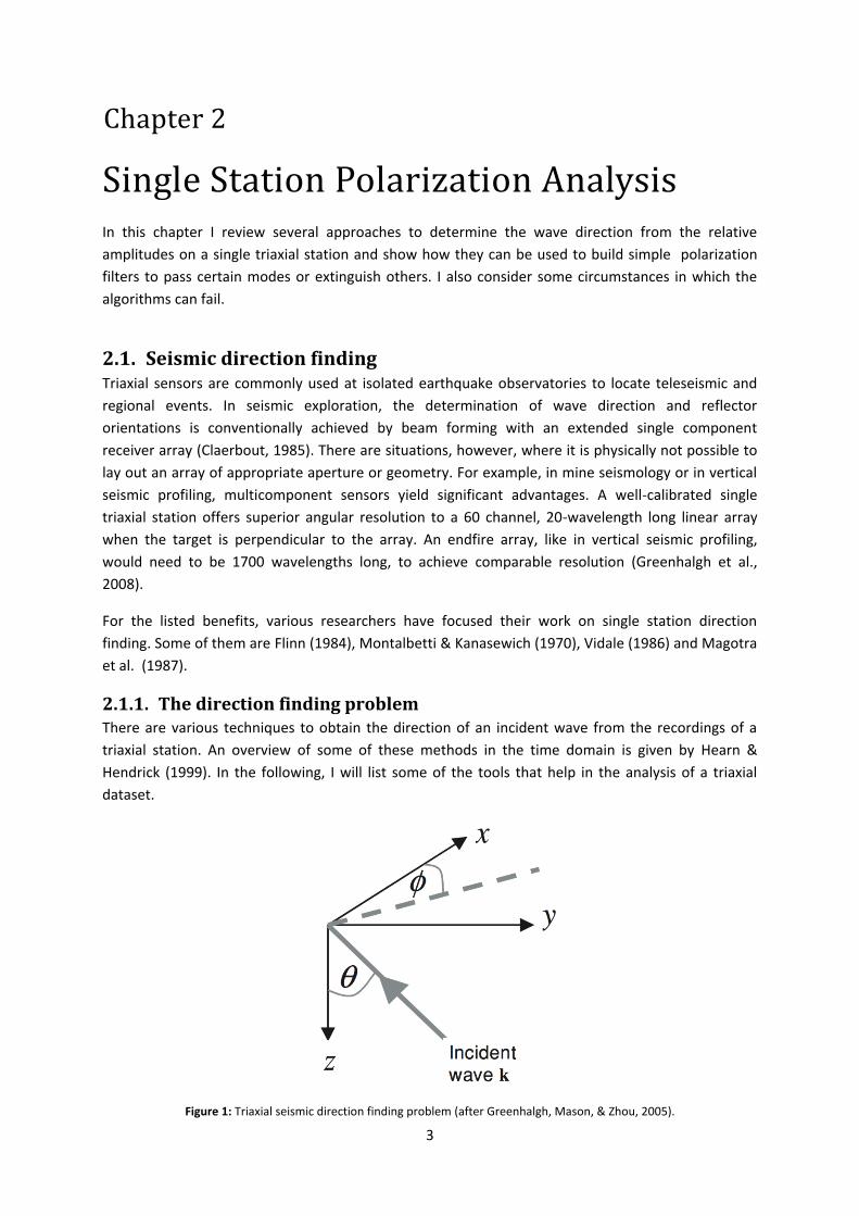
2.1.1. The direction finding problem There are various techniques to obtain the direction of an incident wave from the recordings of a triaxial station. An overview of some of these methods in the time domain is given by Hearn & Hendrick (1999). In the following, I will list some of the tools that help in the analysis of a triaxial dataset.

Figure 1: Triaxial seismic direction finding problem (after Greenhalgh, Mason, & Zhou, 2005).

4

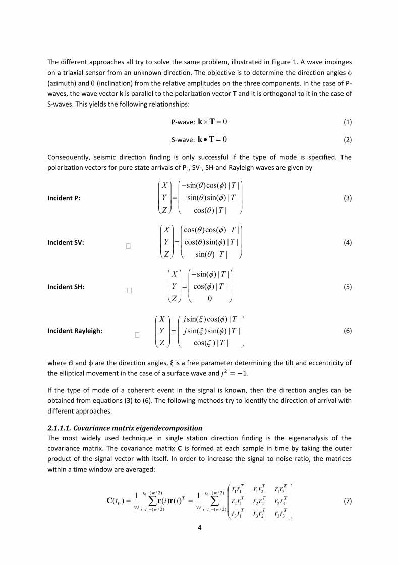
The different approaches all try to solve the same problem, illustrated in Figure 1. A wave impinges on a triaxial sensor from an unknown direction. The objective is to determine the direction angles I (azimuth) and T (inclination) from the relative amplitudes on the three components. In the case of P-waves, the wave vector k is parallel to the polarization vector T and it is orthogonal to it in the case of S-waves. This yields the following relationships:

P-wave: 0 uTk (1)

S-wave: 0 xTk (2)

Consequently, seismic direction finding is only successful if the type of mode is specified. The polarization vectors for pure state arrivals of P-, SV-, SH-and Rayleigh waves are given by

Incident P:

��

XYZ

§�

©�

¨�¨�¨�

·�

¹�

¸�¸�¸�

�sin(T)cos(I) |T |�sin(T)sin(I) |T |cos(T) |T |

§�

©�

¨�¨�¨�

·�

¹�

¸�¸�¸�

(3)

Incident SV:

��

XYZ

§�

©�

¨�¨�¨�

·�

¹�

¸�¸�¸� cos(T)cos(I) |T |cos(T)sin(I) |T |sin(T) |T |

§�

©�

¨�¨�¨�

·�

¹�

¸�¸�¸�

(4)

Incident SH:

��

XYZ

§�

©�

¨�¨�¨�

·�

¹�

¸�¸�¸�

�sin(I) |T |cos(I) |T |

0

§�

©�

¨�¨�¨�

·�

¹�

¸�¸�¸�

(5)

Incident Rayleigh: ¸¸¸

¹

·

¨¨¨

©

§

¸¸¸

¹

·

¨¨¨

©

§

||)cos(||)sin()sin(||)cos()sin(

TTjTj

ZYX

]I[I[

(6)

where Ө and  ф  are  the  direction  angles,  ξ  is  a  free  parameter  determining  the  tilt  and  eccentricity  of  the elliptical movement in the case of a surface wave and 𝑗 = −1.

If the type of mode of a coherent event in the signal is known, then the direction angles can be obtained from equations (3) to (6). The following methods try to identify the direction of arrival with different approaches.

2.1.1.1. Covariance matrix eigendecomposition The most widely used technique in single station direction finding is the eigenanalysis of the covariance matrix. The covariance matrix C is formed at each sample in time by taking the outer product of the signal vector with itself. In order to increase the signal to noise ratio, the matrices within a time window are averaged:

¦¦�

�

�

� ¸¸¸

¹

·

¨¨¨

©

§

)2/(

)2/(332313

322212

312111)2/(

)2/(0

0

0

0

0

1)()(1)(wt

wti TTT

TTT

TTTwt

wti

T

rrrrrrrrrrrrrrrrrr

wii

wt rrC (7)

5

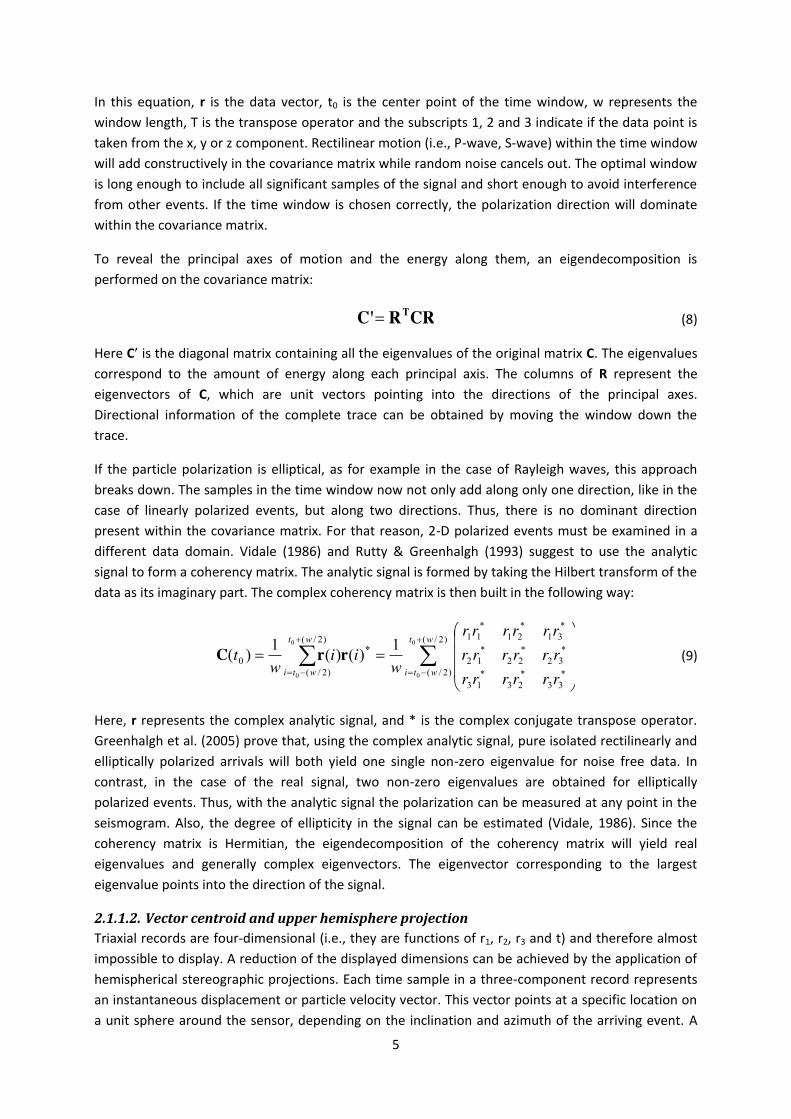
In this equation, r is the data vector, t0 is the center point of the time window, w represents the window length, T is the transpose operator and the subscripts 1, 2 and 3 indicate if the data point is taken from the x, y or z component. Rectilinear motion (i.e., P-wave, S-wave) within the time window will add constructively in the covariance matrix while random noise cancels out. The optimal window is long enough to include all significant samples of the signal and short enough to avoid interference from other events. If the time window is chosen correctly, the polarization direction will dominate within the covariance matrix.

To reveal the principal axes of motion and the energy along them, an eigendecomposition is performed on the covariance matrix:

CRRC' T (8)

Here C’  is  the diagonal matrix containing all the eigenvalues of the original matrix C. The eigenvalues correspond to the amount of energy along each principal axis. The columns of R represent the eigenvectors of C, which are unit vectors pointing into the directions of the principal axes. Directional information of the complete trace can be obtained by moving the window down the trace.

If the particle polarization is elliptical, as for example in the case of Rayleigh waves, this approach breaks down. The samples in the time window now not only add along only one direction, like in the case of linearly polarized events, but along two directions. Thus, there is no dominant direction present within the covariance matrix. For that reason, 2-D polarized events must be examined in a different data domain. Vidale (1986) and Rutty & Greenhalgh (1993) suggest to use the analytic signal to form a coherency matrix. The analytic signal is formed by taking the Hilbert transform of the data as its imaginary part. The complex coherency matrix is then built in the following way:

¦¦�

�

�

� ¸¸¸

¹

·

¨¨¨

©

§

)2/(

)2/( *33

*23

*13

*32

*22

*12

*31

*21

*11)2/(

)2/(0

0

0

0

0

1)()(1)(wt

wti

wt

wti rrrrrrrrrrrrrrrrrr

wii

wt *rrC (9)

Here, r represents the complex analytic signal, and * is the complex conjugate transpose operator. Greenhalgh et al. (2005) prove that, using the complex analytic signal, pure isolated rectilinearly and elliptically polarized arrivals will both yield one single non-zero eigenvalue for noise free data. In contrast, in the case of the real signal, two non-zero eigenvalues are obtained for elliptically polarized events. Thus, with the analytic signal the polarization can be measured at any point in the seismogram. Also, the degree of ellipticity in the signal can be estimated (Vidale, 1986). Since the coherency matrix is Hermitian, the eigendecomposition of the coherency matrix will yield real eigenvalues and generally complex eigenvectors. The eigenvector corresponding to the largest eigenvalue points into the direction of the signal.

2.1.1.2. Vector centroid and upper hemisphere projection Triaxial records are four-dimensional (i.e., they are functions of r1, r2, r3 and t) and therefore almost impossible to display. A reduction of the displayed dimensions can be achieved by the application of hemispherical stereographic projections. Each time sample in a three-component record represents an instantaneous displacement or particle velocity vector. This vector points at a specific location on a unit sphere around the sensor, depending on the inclination and azimuth of the arriving event. A

6

stereographical projection of the points into the equatorial plane yields a scatter plot of azimuth and inclination from all the events present in a specified time window. To preserve amplitude information, the size of each point can be adjusted in such a way that it is proportional to the power content of the projected vector. Time information is hard to include in the display. An attempt to do so can be made by coloring the points according to their time. Obviously, this only makes sense if the amount of observation points is very limited. Otherwise, the display can become too confusing.

Mathematically, the power corresponding to the i-th sample in a record can be expressed by

222iiii ZYXW �� (10)

where X and Y are the horizontal components and Z is the vertical component amplitude. The direction cosines at the same sample are given by

��

li XiWi

i

ii W

Ym

��

ni ZiWi

(11)

The center of gravity of the vector cluster developing on the upper hemisphere of a unit sphere around a triaxial station has the following coordinates:

¦

¦

p

ii

p

iii

W

WlL

1

1

¦

¦

p

ii

p

iii

W

WmM

1

1

¦

¦

p

ii

p

iii

W

WnN

1

1 (12)

Here, p is the number of analyzed samples, excluding samples with negative Z-component, in order to project only on the upper hemisphere. The term Wi makes sure that samples with high signal to noise ratio are weighted more. The direction angles can easily be extracted with the following formulas:

LM

)tan(T (13a) N

LM 22

)tan( � I (13b)

Figure 2: a) Synthetic triaxial record including two P-wave arrivals, corrupted by 50 percent of noise. b) Result of the polarization analysis with the vector centroid method. The angle represents the azimuth and the distance from the center the inclination of arrival direction.

a) b)

7

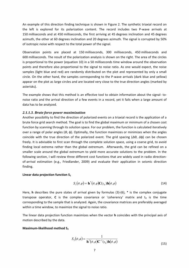
An example of this direction finding technique is shown in Figure 2. The synthetic triaxial record on the left is explored for its polarization content. The record includes two P-wave arrivals at 150 milliseconds and at 450 milliseconds, the first arriving at 45 degrees inclination and 45 degrees azimuth, the other at 60 degrees inclination and 20 degrees azimuth. The signal is corrupted by 50% of isotropic noise with respect to the total power of the signal.

Observation points are placed at 150 milliseconds, 300 milliseconds, 450 milliseconds and 600 milliseconds. The result of the polarization analysis is shown on the right. The area of the circles is proportional to the power (equation 10) in a 50 milliseconds time window around the observation points and therefore also proportional to the signal to noise ratio. As one would expect, the noise samples (light blue and red) are randomly distributed on the plot and represented by only a small circle. On the other hand, the samples corresponding to the P-wave arrivals (dark blue and yellow) appear on the plot as large circles and are located very close to the true direction angles (marked by asterisks).

The example shows that this method is an effective tool to obtain information about the signal- to-noise ratio and the arrival direction of a few events in a record, yet it fails when a large amount of data has to be analyzed.

2.1.1.3. Brute force power maximization Another possibility to find the direction of polarized events on a triaxial record is the application of a brute force grid search method. The goal is to find the global maximum or minimum of a chosen cost function by scanning through its solution space. For our problem, the function is calculated iteratively over a range of polar angles (Ө,  ф).  Optimally,  the  function  maximizes  or  minimizes when the angles coincide with the true direction of the polarized event. The grid spacing (∆Ө, ∆ф)   can   be   chosen  freely. It is advisable to first scan through the complete solution space, using a coarse grid, to avoid finding local extrema rather than the global extremum. Afterwards, the grid can be refined on a smaller scale around the global extremum to yield more accurate solutions to the problem. In the following section, I will review three different cost functions that are widely used in radio direction-of-arrival estimation (e.g., Friedlander, 2009) and evaluate their application in seismic direction finding.

Linear data projection function S1

� � � � � �ITITIT ,,, )( 0*

1 hCh tS (14)

Here, h describes the pure states of arrival given by formulas (3)-(6), * is the complex conjugate transpose operator, C is the complex covariance or 'coherency' matrix and t0 is the time corresponding to the sample that is analyzed. Again, the covariance matrices are preferably averaged within a time window, to maximize the signal to noise ratio.

The linear data projection function maximizes when the vector h coincides with the principal axis of motion described by the data.

Maximum-likelihood method S2

� � � � � �ITIT

IT,,

,)(

1

01*2 hCh t

S � (15)

8

Instead of finding the maximum in a signal space like the linear data projection function, the maximum likelihood method searches for a minimum in an inverse space (i.e., the inverse of the coherency matrix). This minimum corresponds to the direction along the smallest principal axis. The cost function is then formed by taking the reciprocal of this minimizing function and therefore maximizes when the direction is found.

A critical factor in forming this cost function is the inversion of the complex covariance matrix. The covariance matrix of a purely rectilinearly polarized arrival without the presence of any noise is singular and therefore has no inverse. This problem mainly affects synthetic data. In the case of field data there is always a certain amount of noise present. By adding a certain amount of isotropic noise to the data, computational stability can be ensured.

An advantage of the maximum likelihood method is that it takes on very high values when the tested polarization vector is close to the arrival direction, due to the fact that the denominator approaches zero. This results in a display that appears to have a higher resolution than the display of the linear data projection function.

MUSIC-algorithm S3

The multiple signal classification algorithm (MUSIC-algorithm) was introduced by Schmidt (1986). It is a very high-resolution approach that is mainly used in radio direction finding and sonar. It requires an eigendecomposition of the complex covariance matrix, a process that increases computation time. The eigenvectors are sorted in descending order of their eigenvalues, yielding vectors u, v and w. Taking the outer product of the two minimum eigenvectors then forms the following projection matrix:

¸̧¹

·¨̈©

§

¸¸¸

¹

·

¨¨¨

©

§

321

321

3

2

1

3

2

1

wwwvvv

www

vvv

Q (16)

The cost function is given by

� �� � � �ITIT

IT,,

,)(

1

0*3 hQh t

S (17)

Similar to the maximum likelihood method, the null space of the covariance matrix is explored for its minimum. The estimator S3 maximizes when this minimum is found. Due to the non-linearity of the function, it is the most sensitive of the three proposed grid search methods. It is also stable for high signal to noise ratios, since there is no need to compute a matrix inversion.

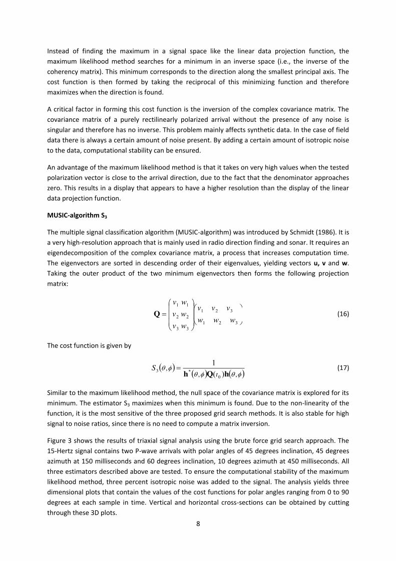
Figure 3 shows the results of triaxial signal analysis using the brute force grid search approach. The 15-Hertz signal contains two P-wave arrivals with polar angles of 45 degrees inclination, 45 degrees azimuth at 150 milliseconds and 60 degrees inclination, 10 degrees azimuth at 450 milliseconds. All three estimators described above are tested. To ensure the computational stability of the maximum likelihood method, three percent isotropic noise was added to the signal. The analysis yields three dimensional plots that contain the values of the cost functions for polar angles ranging from 0 to 90 degrees at each sample in time. Vertical and horizontal cross-sections can be obtained by cutting through these 3D plots.

9

In this way, the polarization properties can be easily tracked over time and over the solution space. In Figure 3, a) shows time slices taken at 150 milliseconds, b) shows time slices taken at 450 milliseconds and c) shows vertical cross-sections through the three dimensional solution space. Warm colors indicate high values of the cost functions and cold colors represent low values. All of the

Figure 3: Analysis of a three-component record using a brute force grid search approach. The record contains two P-wave arrivals at 150 milliseconds (Ө:45,ф:45) and at 450 milliseconds (Ө:60,ф:10). a) Time slices taken at 150 milliseconds. b) Time slices taken at 450 milliseconds. c) Vertical cross-sections through the three-dimensional solution space, showing the evolution of the polarization properties over time. Results for the azimuth are displayed on the left and results for the inclination on the right.

S2

a)

b)

c)

S1 S3

10

three cost functions maximize at the correct angles. Yet, the results from the maximum likelihood method and the MUSIC-algorithm appear to yield better angular resolution than the linear data projection function.

Table 1 shows the computation time that was needed to compute the results in Figure 3 with each of the three estimators on a Lenovo W520 laptop computer with an Intel Core i7-2760QM quadcore CPU and 8 GB of RAM. The matrix inversion that is needed in the maximum likelihood method, makes it the slowest of the three approaches, followed by the MUSIC algorithm where the eigendecomposition of the covariance matrix is the part which consumes the most time. The fastest method is the linear data projection function.

Table 1: Computation time needed to produce the plots in Figure 3

Cost Function Computation Time [s]

Linear data projection function 45 Maximum likelihood method 58

MUSIC-algorithm 50

It was shown that the grid search method is a powerful means of analyzing the polarization properties, despite it being computationally expensive. It can offer very high resolution. This is one of the reasons why exhaustive grid search methods are mainly used in radio direction finding, where ultra high accuracy is desired. In seismic exploration, they are mainly suited for research purposes, where the computation time is not of major importance.

2.1.1.4. Hodograms, semblance and cross correlation The easiest way to display a transient polarized event is to draw a hodogram. It shows motion as a function of time in the X-Y, X-Z and Y-Z planes. Figure 4 shows hodograms of a P-wave coming in at 70 degrees inclination and 20 degrees azimuth, an SV-wave arriving from the same direction and a Rayleigh wave with a free parameter of 45, coming in at 20 degrees azimuth. The rectilinearly polarized events (P- and S-wave) can be easily distinguished from the elliptically polarized Rayleigh wave. If the type of mode is known it is also possible to make estimations of the direction angles directly from the hodogram display.

A more accurate direction estimate for the rectilinearly polarized events can be obtained by a computation of linear regression lines of the hodogram motion. For example, the azimuth can be obtained by fitting a line of Y(t) on X(t) in a least-squares sense. The result would be the same as the one that would be obtained by maximizing the energy in the two-component rotation (Di Siena et al., 1985). The energy is given by

2

1

)]sin()cos([)( ¦

� N

iii YXE III (18)

and the maximum can be found through setting its derivative to zero. In equation (18), Xi and Yi represent the i-th sample of the X- and Y-components, N is the number of samples in the investigated window.

11

Other than by maximizing the energy in the two horizontal components, the azimuth can also be obtained through the analysis of coherency measures like the semblance and the cross correlation. In seismic exploration, these measures are mainly used in the analysis of multichannel single component data (Neidell & Taner, 1971). The principle can be adapted to triaxial trace analysis. Semblance and cross correlation are given by

¦

¦

�

� N

iii

N

iii

yx

yxS

1

22

1

2)()(I (19)

and

Figure 4: Hodograms in the X-Y, X-Z and Y-Z planes representing the noise-free arrivals of a P- (Ө=70,ф=20), an SV- (Ө=70,ф=20) and a Rayleigh (Ө=45,ф=20) wave.

X-Y Plane X-Z Plane Y-Z Plane

Rayleigh:

SV:

P:

12

¦ ¦

¦

N

i

N

iii

N

iii

yx

yxC

1 1

22

1)(I (20)

where

)cos()sin()sin()cos(IIII

iii

iii

YXyYXx

� �

(21)

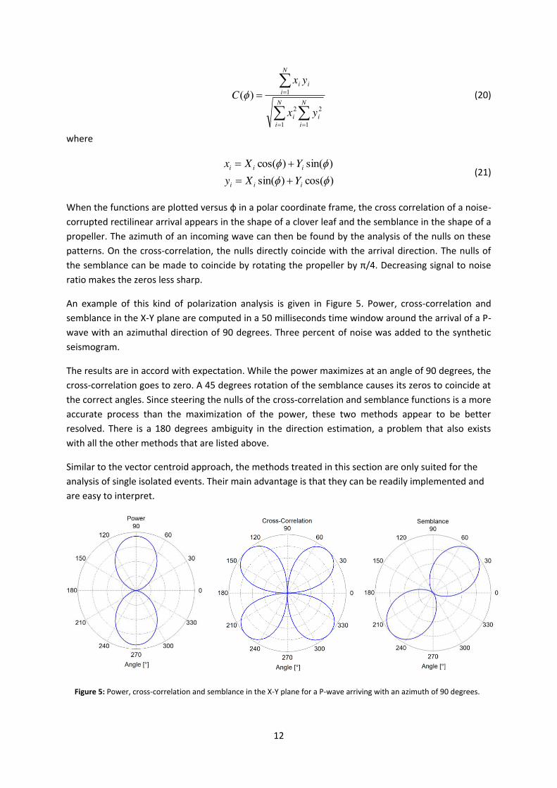
When  the  functions  are  plotted  versus  ф  in  a  polar  coordinate  frame,  the  cross  correlation  of  a  noise-corrupted rectilinear arrival appears in the shape of a clover leaf and the semblance in the shape of a propeller. The azimuth of an incoming wave can then be found by the analysis of the nulls on these patterns. On the cross-correlation, the nulls directly coincide with the arrival direction. The nulls of the semblance can be made to coincide by rotating  the  propeller  by  π/4.  Decreasing  signal  to  noise  ratio makes the zeros less sharp.

An example of this kind of polarization analysis is given in Figure 5. Power, cross-correlation and semblance in the X-Y plane are computed in a 50 milliseconds time window around the arrival of a P-wave with an azimuthal direction of 90 degrees. Three percent of noise was added to the synthetic seismogram.

The results are in accord with expectation. While the power maximizes at an angle of 90 degrees, the cross-correlation goes to zero. A 45 degrees rotation of the semblance causes its zeros to coincide at the correct angles. Since steering the nulls of the cross-correlation and semblance functions is a more accurate process than the maximization of the power, these two methods appear to be better resolved. There is a 180 degrees ambiguity in the direction estimation, a problem that also exists with all the other methods that are listed above.

Similar to the vector centroid approach, the methods treated in this section are only suited for the analysis of single isolated events. Their main advantage is that they can be readily implemented and are easy to interpret.

Figure 5: Power, cross-correlation and semblance in the X-Y plane for a P-wave arriving with an azimuth of 90 degrees.

13

2.1.1.5. Experimental difficulties of single station seismic direction finding Seismic direction finding is prone to errors caused by physical effects and technical aspects. This has to be kept in mind during the interpretation. In the following section, I briefly describe some of the most important problems that can cause the polarization analysis to fail.

Random and coherent noise effects

In the presence of purely random noise (i.e., it is equal in energy on all channels), the eigenanalysis of the covariance matrix theoretically always yields the correct direction estimate, regardless of the signal to noise ratio (Greenhalgh et al., 2008). In practice, this is not the case because the direction finding algorithms all operate within a finite time window. In this window, noise will not cancel out completely. This would only happen if the time window were infinitely long. In a finite time window, the direction estimate will always have an error related to the variance of the noise distribution. Increasing the window length can minimize this error.

Multipathing can cause events to overlap within a time window, resulting in an error in the direction estimation. This error has been quantified by Greenhalgh et al. (2008) for two interfering transient wavelets. They show the effects of relative amplitude, arrival angle and the time delay of the two wavelets. Rutty & Greenhalgh (1993) presented a way to identify overlapping arrivals by forming a two-station 6x6 covariance matrix and correlating events between the stations.

Free-surface effect

The rock-air interface adds a significant complication to the direction finding problem. At this interface, incoming waves are reflected and mode-converted. A sensor mounted at this surface will therefore not only respond to the upgoing event but also, at the same time, to the mode-converted and reflected downgoing events. Thus, the direction that dominates in the signal can significantly differ from the true direction of the incoming wave. For example, if we imagine a P-wave arriving at a flat  free  surface  with  direction  angle  Өp, the triaxial sensor records movement in a different direction with apparent angle TA corresponding to twice the angle of the departing SV waves (Greenhalgh, 2012):

SA TT 2 (22a) PP

SS v

v TT sinsin (22b)

The error becomes larger with increasing angle of incidence.

Kennett (1991) introduced approximate operators that successfully remove the interactions of the free surface from isolated three-component stations for both incoming S- and P- waves. In order for them to work, estimates of slowness and azimuth have to be made. Good results are obtained if information about slowness and azimuth is available from an array of single component sensors collocated with the triaxial station (Jepsen & Kennett, 1990).

Velocity inhomogeneity and anisotropy

Direction finding assumes straight travel paths between the source and the sensor. This assumption is only true for homogeneous media. If the medium is inhomogeneous, ray paths become curvilinear. To locate the source one would need to ray trace back through the medium.

14

Anisotropy can cause the particle motion to differ from the ray direction. To detect the correct direction, it is therefore important to know the velocity structure of the medium and the wavepath of the direct wave.

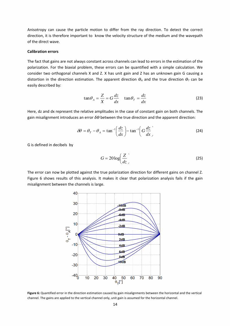
Calibration errors

The fact that gains are not always constant across channels can lead to errors in the estimation of the polarization. For the biaxial problem, these errors can be quantified with a simple calculation. We consider two orthogonal channels X and Z. X has unit gain and Z has an unknown gain G causing a distortion in the direction estimation. The apparent direction ӨA and the true direction ӨT can be easily described by:

dxdzG

XZ

A Ttan dxdz

T Ttan (23)

Here, dz and dx represent the relative amplitudes in the case of constant gain on both channels. The gain misalignment introduces an error δӨ between the true direction and the apparent direction:

¸¹·

¨©§�¸

¹·

¨©§ � ��

dxdzG

dxdz

AT11 tantanTTGT (24)

G is defined in decibels by

¸¹·

¨©§ dzZG log20 (25)

The error can now be plotted against the true polarization direction for different gains on channel Z. Figure 6 shows results of this analysis. It makes it clear that polarization analysis fails if the gain misalignment between the channels is large.

Figure 6: Quantified error in the direction estimation caused by gain misalignments between the horizontal and the vertical channel. The gains are applied to the vertical channel only, unit gain is assumed for the horizontal channel.

15

To prevent errors raised by miswiring or poor mechanical coupling of the sensors, it is essential to extensively test (or calibration) in the field by firing calibration shots in different octants. These errors have to be accounted for in the analysis.

2.2. Single Station Rotation and Polarization Filtering The covariance matrix eigendecomposition approach as discussed in section 2.1.1.1. is not only a useful tool in finding the direction of arrival of an incident wave but it also allows the design of non-linear polarization filters, similar to the filters that are widely used in optics (e.g., Born & Wolf 1975). The analysis of the covariance matrix yields three eigenvectors representing the principal axes of motion. The power in each of these directions is given by the eigenvalues. For isolated noise-free rectilinear arrivals, all of the energy is expected to be in the direction (eigenvector) corresponding to the largest eigenvalue. In the case of an isolated surface wave, energy will be present in two directions, corresponding to the axes of the polarization ellipsoid. Ratios of the eigenvalues therefore provide information on the degree of polarization and the rectilinearity or ellipticity of the signal. This fact can be exploited to build polarization filters that suppress or enhance certain modes.

A very simple polarization filter that enhances signal amplitudes is the rotation of the data into the coordinate frame that is described by its principal axes of motion. This is easily achieved by forming the dot product of the data vector with the three eigenvectors of its covariance matrix:

1i eR x iX 2eRi x iY 3eRi x iZ (26)

Ri is the data vector at the i-th sample. e1 ,e2 and e3 are the eigenvectors sorted in descending order of their corresponding eigenvalues. The data is represented in its new coordinate frame by Xi, Yi and Zi.

A common application of this technique is the rotation of the horizontal components into the direction of the source. This can become a necessity if the geophones in the field are not all oriented in the same way. For example, in a VSP the geophones are often lowered down the borehole on a chain. This chain can get twisted so that each geophone is oriented differently in the vertical borehole. The reorientation is achieved by rotating each geophone individually. To do so, a 2x2 covariance matrix has to be formed within a time window around the first breaks. Each sample of the trace is then projected onto the principal eigenvector of this covariance matrix by forming the dot product. A real data example of this procedure is given in section 2.3.

More complex polarization filters can be built using polarization parameters. Various researchers have proposed different measures of polarization (e.g., Montalbetti & Kanasewich, 1970; Vidale, 1986; Cichowisz et al., 1988) . Esmersoy (1984) proposed the following polarization parameter P:

¦

¸̧¹

·¨̈©

§�

�

3

132

1 12

iiP O

OOO

(27)

where  λ1,  λ2 and  λ3 are the eigenvalues of the covariance matrix sorted in descending order. If there is no polarization, all three eigenvalues are equal to each other and P becomes zero, otherwise P increases linearly with increasing linearly polarized power. Following Born & Wolf (1975) the degree of polarization can then be expressed by

16

1�

PPB (28)

B is zero for unpolarized signals and unity for completely polarized signals. It can be used as a gain function to suppress weakly polarized signals and random noise.

Vidale (1986) used the analytic signal and the complex covariance matrix to introduce a measure of ellipticity. It is built from the complex eigenvector e1 corresponding  to  the  largest  eigenvalue  λ1. Since the phase in the complex plane of the eigenvectors is initially arbitrary, e1 has to be rotated by the angle that maximizes the length of its real component. In practice, this is achieved by maximizing function  X  by  a  search  over  α=0°-180°:

222 ))(Re())(Re())(Re( DDD ciseciseciseX zyx �� (29)

where Re(x) is the real part of x, cisα is cosα+isinα  and the components of e1 are given by ex, ,ey and ez. The eigenvector is then rotated by the angle that maximizes X. The elliptical component of polarization can then be estimated by

XXPE21�

(30)

Since the eigenvector is a unit vector, 21 X� is the length of the imaginary component of e1 and

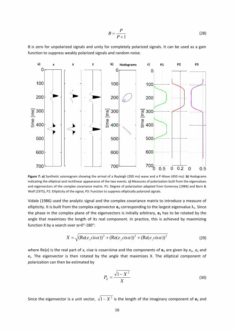
Figure 7: a) Synthetic seismogram showing the arrival of a Rayleigh (200 ms) wave and a P-Wave (450 ms). b) Hodograms indicating the elliptical and rectilinear appearance of the two events. c) Measures of polarization built from the eigenvalues and eigenvectors of the complex covariance matrix. P1: Degree of polarization adapted from Esmersoy (1984) and Born & Wolf (1975), P2: Ellipticity of the signal, P3: Function to suppress elliptically polarized signals.

x y z Hodograms P3 P1 P2 a) b) c)

17

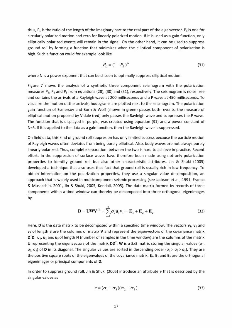
thus, PE is the ratio of the length of the imaginary part to the real part of the eigenvector. PE is one for circularly polarized motion and zero for linearly polarized motion. If it is used as a gain function, only elliptically polarized events will remain in the signal. On the other hand, it can be used to suppress ground roll by forming a function that minimizes when the elliptical component of polarization is high. Such a function could for example look like

NEL PP )1( � (31)

where N is a power exponent that can be chosen to optimally suppress elliptical motion.

Figure 7 shows the analysis of a synthetic three component seismogram with the polarization measures P1, P2 and P3 from equations (28), (30) and (31), respectively. The seismogram is noise free and contains the arrivals of a Rayleigh wave at 200 milliseconds and a P wave at 450 milliseconds. To visualize the motion of the arrivals, hodograms are plotted next to the seismogram. The polarization gain function of Esmersoy and Born & Wolf (shown in green) passes both events, the measure of elliptical motion proposed by Vidale (red) only passes the Rayleigh wave and suppresses the P wave. The function that is displayed in purple, was created using equation (31) and a power constant of N=5. If it is applied to the data as a gain function, then the Rayleigh wave is suppressed.

On field data, this kind of ground roll suppresion has only limited success because the particle motion of Rayleigh waves often deviates from being purely elliptical. Also, body waves are not always purely linearly polarized. Thus, complete separation between the two is hard to achieve in practice. Recent efforts in the suppression of surface waves have therefore been made using not only polarization properties to identify ground roll but also other characteristic attributes. Jin & Shuki (2005) developed a technique that also uses that fact that ground roll is usually rich in low frequency. To obtain information on the polarization properties, they use a singular value decomposition, an approach that is widely used in multicomponent seismic processing (see Jackson et al., 1991; Franco & Musacchio, 2001, Jin & Shuki, 2005, Kendall, 2005). The data matrix formed by records of three components within a time window can thereby be decomposed into three orthogonal eigenimages by

¦

�� 3

12

ii 31ii

T EEEvuUWVD V (32)

Here, D is the data matrix to be decomposed within a specified time window. The vectors v1, v2 and

v3 of length 3 are the columns of matrix V and represent the eigenvectors of the covariance matrix DTD. u1, u2 and u3 of length N (number of samples in the time window) are the columns of the matrix U representing the eigenvectors of the matrix DDT. W is a 3x3 matrix storing the singular values (σ1, σ2, σ3) of D in  its  diagonal.  The  singular  values  are  sorted  in  descending  order  (σ1 >  σ2 > σ3). They are the positive square roots of the eigenvalues of the covariance matrix. E1, E2 and E3 are the orthogonal eigenimages or principal components of D.

In order to suppress ground roll, Jin & Shuki (2005) introduce an attribute e that is described by the singular values as

))(( 3231 VVVV �� e (33)

18

The attribute e is the area of the major principal section of the polarization ellipsoid, adjusted by the minor   semi   axis   σ3. An advantage of e is that it includes amplitude information. Ground roll has usually much higher amplitudes than body waves, a fact which helps in the distinction of the two. Using attribute e, filtered data F can be obtained by

)()1( 21 EEDDF ���� gg (34)

where D is the original data matrix and E1 and E2 are the first two eigenimages of the data matrix after the application of a low pass filter. The quantity g is an integer that indicates if ground roll is present in the time window: g = 1 if e>eg and g=0 otherwise. Quantity eg is a threshold value of e above which the ground roll is most likely present. It can be obtained by sorting e in ascending order. eg can then be identified as the value above which e increases rapidly.

This method uses three characteristic attributes of surface waves to obtain an optimal result: the low-frequency content, the high amplitudes and the elliptical polarization. A real data example of this technique is given in section 2.3. Even better signal can be preserved if more than one station is used in the analysis. However, this is only possible if the distance between neighboring stations is short enough to ensure that the ground roll properties do not change much between them.

2.3. Real Data examples The conditions in the field often deviate considerably from some of the assumptions that were made in this chapter. Thus, it is important to test the applicability of the proposed algorithms on field data. In this section, I give two examples of single station polarization processing on real datasets that were provided by the National Cooperative for the Disposal of Radioactive Waste (Nagra). The MATLAB codes that are used in this analysis were developed as a part of this project and base on the theory that was discussed in this chapter.

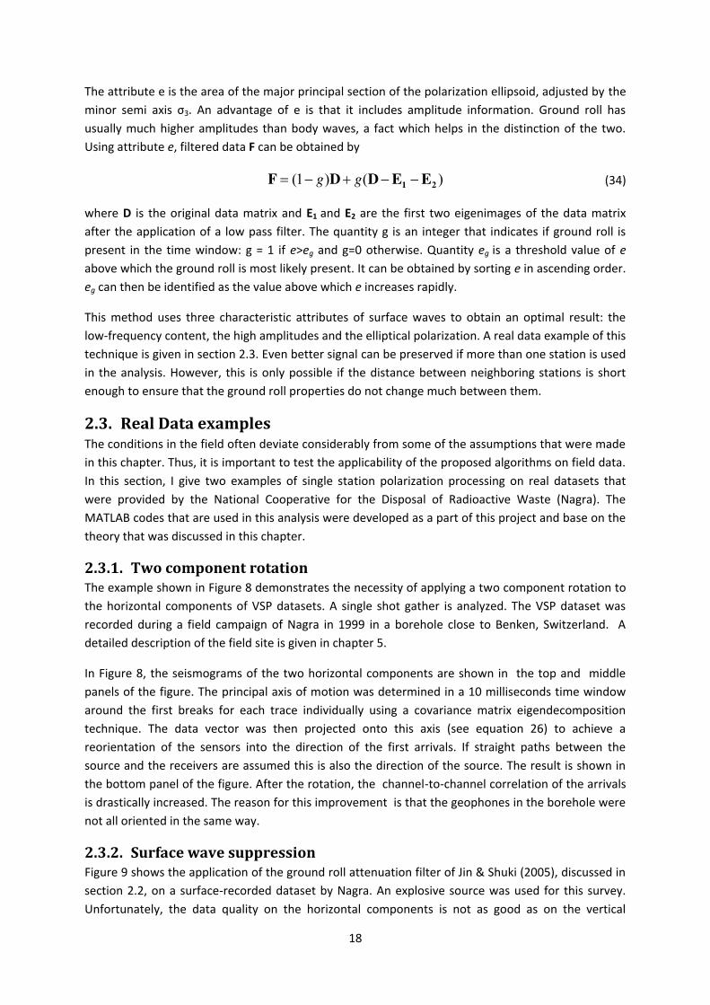
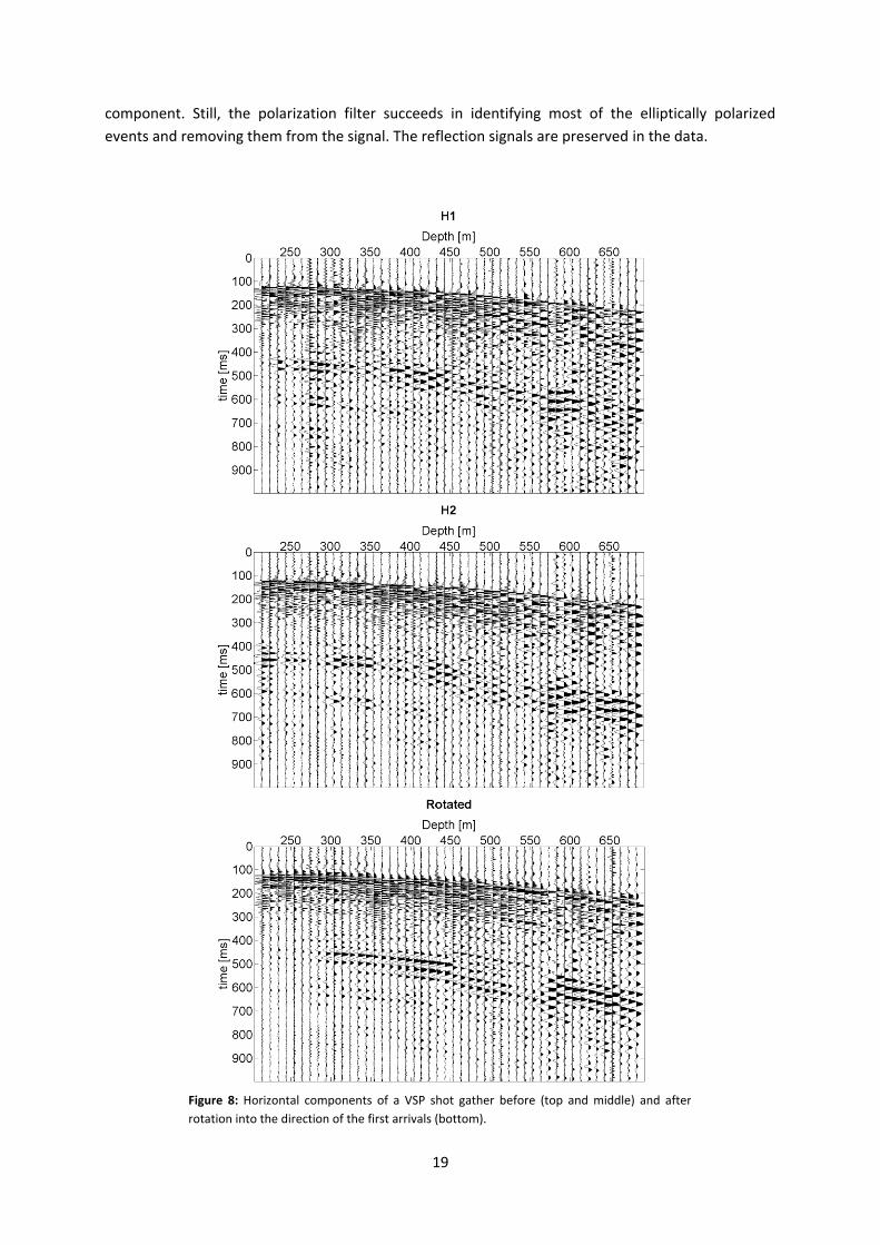
2.3.1. Two component rotation The example shown in Figure 8 demonstrates the necessity of applying a two component rotation to the horizontal components of VSP datasets. A single shot gather is analyzed. The VSP dataset was recorded during a field campaign of Nagra in 1999 in a borehole close to Benken, Switzerland. A detailed description of the field site is given in chapter 5.

In Figure 8, the seismograms of the two horizontal components are shown in the top and middle panels of the figure. The principal axis of motion was determined in a 10 milliseconds time window around the first breaks for each trace individually using a covariance matrix eigendecomposition technique. The data vector was then projected onto this axis (see equation 26) to achieve a reorientation of the sensors into the direction of the first arrivals. If straight paths between the source and the receivers are assumed this is also the direction of the source. The result is shown in the bottom panel of the figure. After the rotation, the channel-to-channel correlation of the arrivals is drastically increased. The reason for this improvement is that the geophones in the borehole were not all oriented in the same way.

2.3.2. Surface wave suppression Figure 9 shows the application of the ground roll attenuation filter of Jin & Shuki (2005), discussed in section 2.2, on a surface-recorded dataset by Nagra. An explosive source was used for this survey. Unfortunately, the data quality on the horizontal components is not as good as on the vertical

19

component. Still, the polarization filter succeeds in identifying most of the elliptically polarized events and removing them from the signal. The reflection signals are preserved in the data.

Figure 8: Horizontal components of a VSP shot gather before (top and middle) and after rotation into the direction of the first arrivals (bottom).

20

Figure 9: Ground roll attenuation achieved by a non-linear polarization filter using singular value decomposition. a) Input data of the vertical (Z) and horizontal (H1,H2) components. b) output of the polarization filter algorithm.

a) b)

c) d)

e) f)

21

3Chapter 3

Array Polarization Analysis One of the major drawbacks of single station polarization analysis, as discussed in chapter 2, is its inability to deal with more than one arrival within the analyzed time window. By extending the analysis to an array of multicomponent sensors, moveout characteristics can be exploited simultaneously with polarization properties to build filters that are able to separate the wavefield.

Gal'perin (1983) introduced the term polarization-position correlation (PPC) for this kind of analysis. He proposed a method to separate P- and S-waves by tracking the polarization properties of arrivals along the line of geophones. Dankbaar (1985) developed a filter that removes the effect of the geophone receiving characteristics to obtain separated P- and S-wave seismograms. His filter operates in f-k space whereas the approach of Gal'perin operates in t-x space. Both methods require constant velocity along the receiver array. Foster & Gaiser (1985) suggested a method that can handle velocity variations along the array. This is achieved by the use of a Radon transform. Isolated P- and S-wave sections are obtained by applying a variable rotation operator to the data as they are multi-component projected into Radon space. This idea was exploited and extended by Greenhalgh et al. (1990) who suggested to compute in addition to the pass plane energy the amount of energy spillover in the so-called extinction planes and apply a non-linear 2-D gain function to enhance strongly polarized pixels in Radon space.

In this chapter, I review the method of Greenhalgh et al. (1990) and show its performance on synthetic data. Since the method operates in tau-p space, the chapter includes a section on the theory of the discrete Radon transform.

3.1. Theory of the discrete Radon transform In seismic exploration, the Radon transform is more commonly known as slant-stacking,   the   τ-p transform or the velocity stacking method (Yilmaz, 2008). It is mainly used in the suppression of multiple reflections (Foster & Mosher, 1992; Kabir & Marfurt, 1999) as well as ground roll and random noise (Russel et al., 1990). The linear Radon transform stacks two dimensional datasets along straight lines of different slopes p and intercept times τ.   The   energy   along   each   line   is   then  represented  by  a  pixel  in  τ-p space. Overlapping events in t-x space may separate in tau-p space. This is the reason for the popularity of the Radon transform in seismic data processing. Detailed formulations of the forward and inverse discrete Radon transform are given by Beylkin (1987) and Foster & Mosher (1992). Both use a least-squares inversion approach to improve the focusing abilities of the transform. Zhou & Greenhalgh (1994) suggested a convolutional approach to derive the transform pairs. Based on these studies, it is shown in the following section how seismic data can be projected from time-distance space to tau-p space and vice versa.

For continuous seismic data F(x,t), the Radon transform A(p,τ) is defined by

³f

f�

� dxpxxFpA ),(),( WW (35)

22

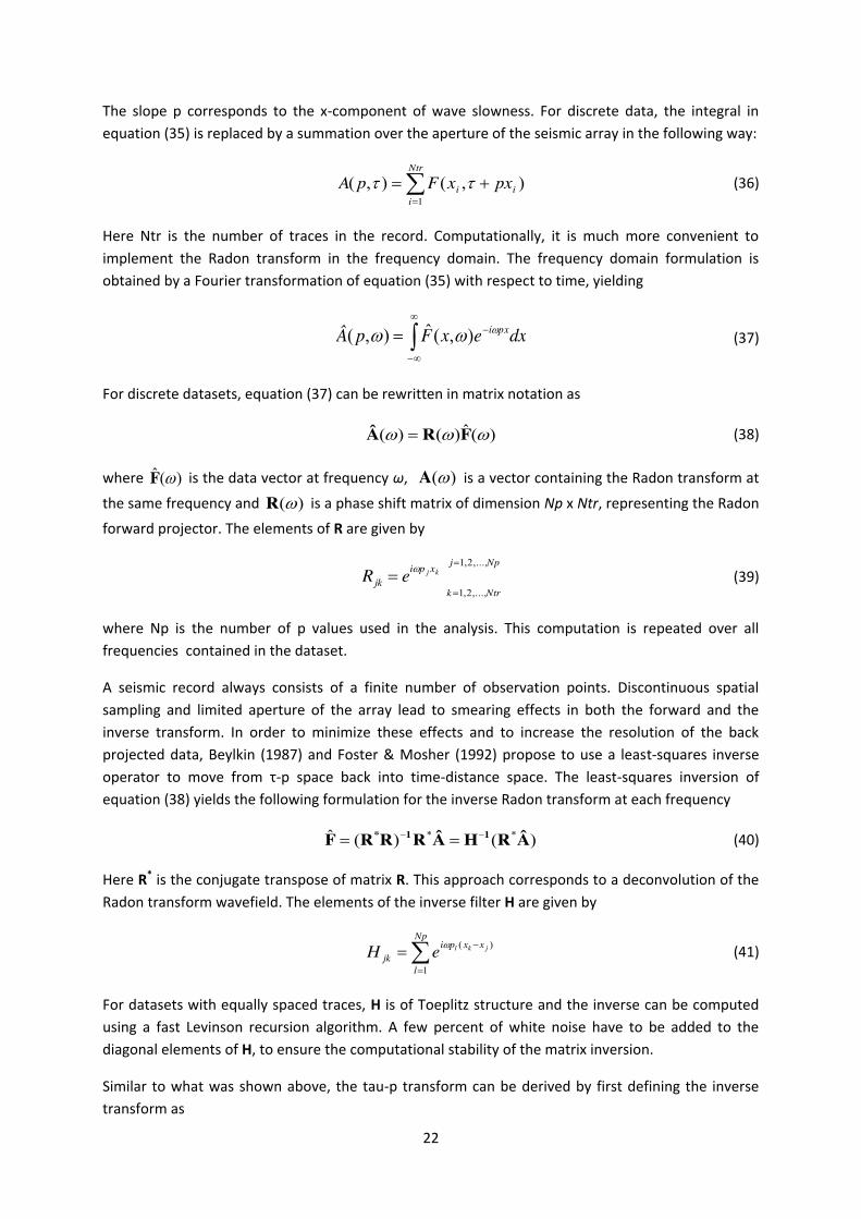
The slope p corresponds to the x-component of wave slowness. For discrete data, the integral in equation (35) is replaced by a summation over the aperture of the seismic array in the following way:

¦

� Ntr

iii pxxFpA

1

),(),( WW (36)

Here Ntr is the number of traces in the record. Computationally, it is much more convenient to implement the Radon transform in the frequency domain. The frequency domain formulation is obtained by a Fourier transformation of equation (35) with respect to time, yielding

³f

f�

� dxexFp pxiZZZ ),(ˆ),( (37)

For discrete datasets, equation (37) can be rewritten in matrix notation as

)(ˆ)()( ZZZ FRÂ (38)

where )(ˆ ZF is the data vector at frequency ω, )(ZÂ is a vector containing the Radon transform at

the same frequency and )(ZR is a phase shift matrix of dimension Np x Ntr, representing the Radon

forward projector. The elements of R are given by

kj xpijk eR Z

Npj

Ntrk

,...,2,1

,...,2,1

(39)

where Np is the number of p values used in the analysis. This computation is repeated over all frequencies contained in the dataset.

A seismic record always consists of a finite number of observation points. Discontinuous spatial sampling and limited aperture of the array lead to smearing effects in both the forward and the inverse transform. In order to minimize these effects and to increase the resolution of the back projected data, Beylkin (1987) and Foster & Mosher (1992) propose to use a least-squares inverse operator   to   move   from   τ-p space back into time-distance space. The least-squares inversion of equation (38) yields the following formulation for the inverse Radon transform at each frequency

)()(ˆ ** ÂRHÂRRRF 11* �� (40)

Here R* is the conjugate transpose of matrix R. This approach corresponds to a deconvolution of the Radon transform wavefield. The elements of the inverse filter H are given by

¦

� Np

l

xxpijk

jkleH1

)(Z (41)

For datasets with equally spaced traces, H is of Toeplitz structure and the inverse can be computed using a fast Levinson recursion algorithm. A few percent of white noise have to be added to the diagonal elements of H, to ensure the computational stability of the matrix inversion.

Similar to what was shown above, the tau-p transform can be derived by first defining the inverse transform as

23

)()()(ˆ * ZZZ ÂRF (42)

A least squares inversion of this formula leads to the following formulation for the forward transform

)ˆ(ˆ)( 1* FRQFRRR 1�� (43)

If the increment between the p values is chosen to be constant, Matrix Q will always be of Toeplitz structure and the inverse can be computed using the Levinson recursion. Equation (43) compensates for the finite length of the array by a p-direction deconvolution. The forward transform derived with this approach will therefore provide better resolution in 𝜏-p space than the forward transform formulated in equation (38). This is of particular interest in the filtering of multiples and ground roll where high resolution in τ-p space is desired. For the specific problem that concerns us in this chapter (i.e., the separation of the wavefield), it is of lower importance. High resolution is not necessarily required in Radon space but in the reconstructed data that represents the separated wavefield. Thus, the computer scripts accompanying this thesis are based on the transform pair given by equations (38) and (40).

3.1.1. Aliasing in the Radon transform Some sampling conditions have to be fulfilled to avoid aliasing in the τ-p transform. Graphical illustrations and mathematical formulations of these conditions were given by Turner (1990).

For a symmetrical range of p-values, the maximum p value contained in the analysis pmax (=-pmin) must not exceed a limit imposed by the temporal and spatial sampling of the data. This limit is given by

max

max 21xf

p'

d (44)

Here  ∆x  is  the  trace spacing and fmax is the maximum frequency contained in the data. Reducing  ∆x  by trace interpolation can help avoid aliasing caused by a violation of this inequation (Kabir & Marfurt, 1999).

Aliasing can also occur if the sampling is insufficient in p direction. The condition to avoid this problem is given by

max

1fx

pr

�' (45)

Here  ∆p  is  the  increment  between  the  p  values  and  xr is the aperture of the seismic array. Thus, the resolution  of  the  Radon  transform  can  often  be  increased  by  choosing  a  small  value  for  ∆p.  Of  course,  this comes at the cost of longer computation times.

Further resolution improvements of the Radon transform can be achieved by tapering the far offsets of the seismic dataset and by the introduction of weighting terms to account for unequal spatial sampling (Kabir & Marfurt, 1999).

24

3.2. Controlled direction reception filtering (CDR) Gal'perin (1983) distinguished between two observation systems for the discrimination of the seismic wavefield. He called them controlled direction reception (CDR) of type 1 and type 2. CDRI describes the wavefield at a point with regard to its polarization while CDRII describes the wavefield in a volume or a plane with respect to its apparent velocity. The wavefield separation algorithms proposed by Greenhalgh et al. (1990) use both systems in order to achieve an optimal result.

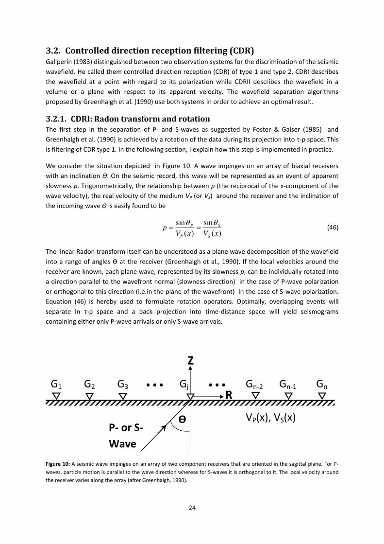
3.2.1. CDRI: Radon transform and rotation The first step in the separation of P- and S-waves as suggested by Foster & Gaiser (1985) and Greenhalgh et al. (1990) is achieved by a rotation of the data during its projection into τ-p space. This is filtering of CDR type 1. In the following section, I explain how this step is implemented in practice.

We consider the situation depicted in Figure 10. A wave impinges on an array of biaxial receivers with an inclination Ө. On the seismic record, this wave will be represented as an event of apparent slowness p. Trigonometrically, the relationship between p (the reciprocal of the x-component of the wave velocity), the real velocity of the medium VP (or VS) around the receiver and the inclination of the incoming wave Ө is easily found to be

)(

sin)(

sinxVxV

pS

S

P

P TT (46)

The linear Radon transform itself can be understood as a plane wave decomposition of the wavefield into  a  range  of  angles  Ө  at  the  receiver  (Greenhalgh  et  al.,  1990).   If   the   local  velocities  around  the  receiver are known, each plane wave, represented by its slowness p, can be individually rotated into a direction parallel to the wavefront normal (slowness direction) in the case of P-wave polarization or orthogonal to this direction (i.e.in the plane of the wavefront) in the case of S-wave polarization. Equation (46) is hereby used to formulate rotation operators. Optimally, overlapping events will separate   in   τ-p space and a back projection into time-distance space will yield seismograms containing either only P-wave arrivals or only S-wave arrivals.

Figure 10: A seismic wave impinges on an array of two component receivers that are oriented in the sagittal plane. For P-waves, particle motion is parallel to the wave direction whereas for S-waves it is orthogonal to it. The local velocity around the receiver varies along the array (after Greenhalgh, 1990).

R

VP(x), VS(x)

Z

Ө

G1 G3 G2 Gn-2 Gn-1 Gn Gj

P- or S-Wave

... ...

25

Mathematically, the simultaneous Radon transform and rotation to pass P-waves or S-waves, respectively, can be expressed by

> @³ ³f

f�

f

f�

��� � dxpxxHpxxZdxpxxFpA PPPP ),(sin),(cos),(),( WTWTWW (47)

> @³ ³f

f�

f

f�

���� � dxpxxHpxxZdxpxxFpA SSSS ),(cos),(sin),(),( WTWTWW (48)

where Z(x,t) is the data of the vertical component and H(x,t) is the data of the radial horizontal component. H(x,t) is usually obtained by a rotation of the horizontal components of a three component record into the sagittal source-receiver plane (see section 2.2.).

The rotation operators contained in equations (47) and (48) are obtained from equation (46) in the

following way (using the trigonometric identity 1)(cos)(sin 22 � TT ):

)(sin xpVPP T (49a) )(1cos 22 xVp PP � T (49b)

)(sin xpVSS T (50a) )(1cos 22 xVp SS � T (50b)

If the receivers are mounted at the surface, the rotation operators have to be adapted to account for the free surface effect (see section 2.1.1.5.). Detailed formulations of the rotation operators under these circumstances are given by Greenhalgh et al. (1990).

For discrete datasets in the frequency domain, equations (47) and (48) can be rewritten in matrix notation as

)(ˆ)()(ˆ)()( ZZZZZ HNZMÂP � (51)

)(ˆ)()(ˆ)()( ZZZZZ HPZOÂS � (52)

where the elements of the projection matrices M ,N ,O and P are given by

kj xpikPjjk exVpM Z)(1 22� (53a) kj xpi

kPjjk exVpN Z)( (53b)

kj xpikSjjk exVpO Z)(� (54a) kj xpi

kSjjk exVpP Z)(1 22� (54b)

Here kj xpie Zcorresponds to the elements of the Radon forward projector R given in equation (39),

j=1,2,3, ... ,Np and k=1,2,3, ... ,Ntr. This computation is repeated over all the frequencies in the dataset to obtain the 'pass planes' ÂP and ÂS for P- and S- waves   in  ω-p space. An inverse Fourier transform of ÂP and ÂS with  respect  to  frequency  yields  the  'pass  planes'  in  τ-p space.

In practice, various factors can cause P-wave energy to leak over into the S-wave pass plane and vice versa. This leads to flawed reconstructions of the P- and S-wave seismograms. Reasons for this energy spill-over can be the presence of noise, mode-conversions, near-field diffractions, anisotropy,

26

inaccurate information of the local velocity structure or aliasing and artifacts in the Radon transform (see section 3.1.1.). Also, there is always a range of slowness values associated with each mode. In order to minimize these effects, further processing steps are required.

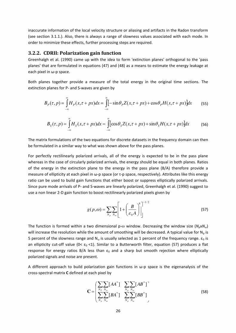
3.2.2. CDRII: Polarization gain function Greenhalgh et al. (1990) came up with the idea to form 'extinction planes' orthogonal to the 'pass planes' that are formulated in equations (47) and (48) as a means to estimate the energy leakage at each  pixel  in  ω-p space.

Both planes together provide a measure of the total energy in the original time sections. The extinction planes for P- and S-waves are given by

> @³ ³f

f�

f

f�

���� � dxpxxHpxxZdxpxxHpB PPPP ),(cos),(sin),(),( WTWTWW (55)

> @³ ³f

f�

f

f�

��� � dxpxxHpxxZdxpxxHpB SSSS ),(sin),(cos),(),( WTWTWW (56)

The matrix formulations of the two equations for discrete datasets in the frequency domain can then be formulated in a similar way to what was shown above for the pass planes.

For perfectly rectilinearly polarized arrivals, all of the energy is expected to be in the pass plane whereas in the case of circularly polarized arrivals, the energy should be equal in both planes. Ratios of the energy in the extinction plane to the energy in the pass plane (B/A) therefore provide a measure  of  ellipticity  at  each  pixel  in  ω-p  space  (or  τ-p space, respectively). Attributes like this energy ratio can be used to build gain functions that either boost or suppress elliptically polarized arrivals. Since pure mode arrivals of P- and S-waves are linearly polarized, Greenhalgh et al. (1990) suggest to use a non linear 2-D gain function to boost rectilinearly polarized pixels given by

2/18

0

1),(

�

¦¦»»¼

º

««¬

ª¸̧¹

·¨̈©

§�

pN N ABpg

ZH

Z (57)

The function is formed within a two dimensional p-Z window. Decreasing the window size (NpxNω) will increase the resolution while the amount of smoothing will be decreased. A typical value for Np is 5 percent of the slowness range and Nω is  usually  selected  as  1  percent  of  the  frequency  range.  ε0 is an ellipticity cut-off   value   (0<   ε0 <1). Similar to a Butterworth filter, equation (57) produces a flat response   for   energy   ratios   B/A   less   than   ε0 and a sharp but smooth rejection where elliptically polarized signals and noise are present.

A   different   approach   to   build   polarization   gain   functions   in   ω-p space is the eigenanalysis of the cross-spectral matrix C defined at each pixel by

¸¸¸

¹

·

¨¨¨

©

§

¦¦¦¦¦¦¦¦

pp

pP

N NN N

N NN N

BBBA

ABAA

ZZ

ZZ

][][

][][

**

**

C (58)

27

where * is the complex conjugate operator. Different measures of rectilinearity and ellipticity can be derived from the eigenvalues of matrix C. An overview over some of these measures is given in section 2.2.

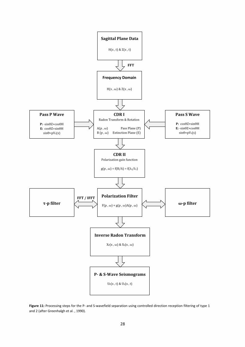
This  kind  of    polarization  filtering  in  ω-p space is a CDR type 2 process. An overview over all the steps in the wavefield separation process is given in Figure 11.

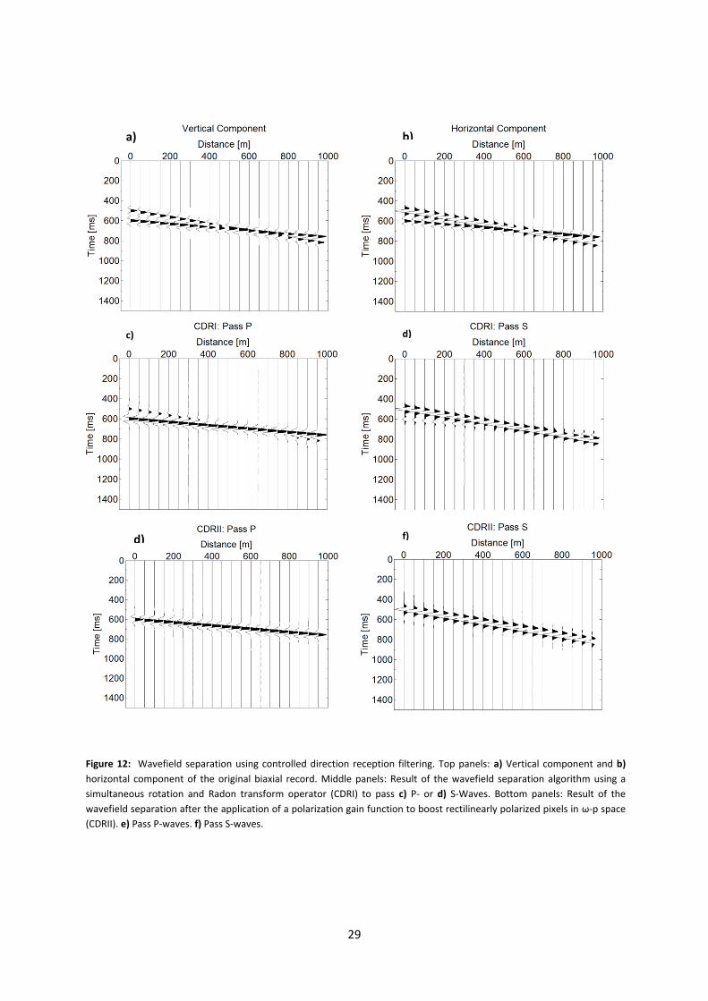
3.3. Synthetic Data Examples A simple example of the wavefield separation technique of Greenhalgh et al. (1990) is shown in Figure 12. Analyzed is a biaxial record showing two interfering waves traveling along the array: A P-wave with an apparent velocity of 6 m/ms and an S-wave with an apparent velocity of 3 m/ms. The actual velocity of the medium is 3 m/ms for P-waves and 2 m/ms for S-waves. Using the relationship in equation (46), the angles of inclination of the two arrivals are easily found to be 30 degrees in the case of the P-wave and 41.81 degrees in the case of the S-wave.

The CDRI process partially separates the wavefield. Some energy spill over from the other (undesired) mode can still be observed. This effect is removed by the application of a two dimensional  polarization  gain  function  in  ω-p space (equation 57). An ellipticity cut-off  value  ε0 of 0.3 was used in this step. After this CDRII filtering process, clean isolated P- and S-wave sections are obtained. This result was achieved using a total number of 51 p values in the range of 0 to 0.5 ms/m.

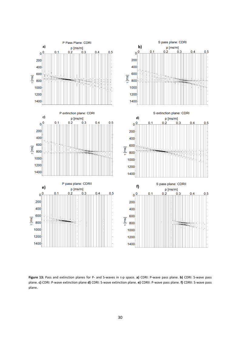
For the same record, Figure 13 shows the pass planes for P- and S-waves   in   τ-p space before and after polarization filtering as well as the extinction planes used in the design of the filters. The events appear to be better focused after the application of the polarization filter (CDRII), energy leaking over from other modes is suppressed.

An example to demonstrate the random noise suppression capabilities of the method is given in Figure 14. It shows the analysis of the same record as in Figure 12 but this time, the signal is corrupted by 70% of isotropic noise on the vertical component and 50% on the horizontal component. Here the noise power is given in percentage of the total signal power. The result is obtained using the same Radon transform parameters as before and an ellipticity cut-off value ε0 of 0.1. The filtered output shows not only a successful separation of the wavefield but also a clear reduction in random noise.

28

Sagittal Plane Data

H(x , t) & Z(x , t)

CDR I Radon Transform & Rotation

A(p , ω) Pass Plane (P) B (p , ω) Extinction Plane (E)

Inverse Radon Transform

XP(x , ω) & XS(x , ω)

CDR II Polarization gain function

g(p , ω) = f(B/A) = f(λ2/λ1)

P- & S-Wave Seismograms

UP(x , t) & US(x , t)

Polarization Filter

F(p , ω) = g(p , ω)A(p , ω)

Pass P Wave

P: -sinӨZ+cosӨH E: cosӨZ+sinӨH sinӨ=pVS(x)

Pass S Wave

P: cosӨZ+sinӨH E: -sinӨZ+cosӨH

sinӨ=pVS(x)

Frequency Domain

H(x , ω) & Z(x , ω)

ω-p filter

τ-p filter

FFT / IFFT

FFT

Figure 11: Processing steps for the P- and S-wavefield separation using controlled direction reception filtering of type 1 and 2 (after Greenhalgh et al. , 1990).

29

a) b)

c) d)

d) f)

Figure 12: Wavefield separation using controlled direction reception filtering. Top panels: a) Vertical component and b) horizontal component of the original biaxial record. Middle panels: Result of the wavefield separation algorithm using a simultaneous rotation and Radon transform operator (CDRI) to pass c) P- or d) S-Waves. Bottom panels: Result of the wavefield separation after the application of a polarization gain function to boost rectilinearly polarized pixels in ω-p space (CDRII). e) Pass P-waves. f) Pass S-waves.

30

Figure 13: Pass and extinction planes for P- and S-waves in τ-p space. a) CDRI: P-wave pass plane. b) CDRI: S-wave pass plane. c) CDRI: P-wave extinction plane d) CDRI: S-wave extinction plane. e) CDRII: P-wave pass plane. f) CDRII: S-wave pass plane.

b)

c) d)

e) f)

a)

31

a) b)

c) d)

Figure 14: a) Vertical component of biaxial record corrupted by 70% of random noise. b) Horizontal component of the record with 50% of random noise. c) Output P-section of the wavefield separation algorithm. d) Output S-section of the wavefield separation algorithm.

32

33

4 Chapter 4

Multicomponent Migration P- and S-waves provide different, albeit complementary information on the petrophysical properties of a geological target. Especially in the study of anisotropy, maps obtained by shear wave imaging can provide significantly more information than a conventionally migrated P-wave image (Crampin, 1985).

Usually, P- and S-wavefields are separated before they are put through a scalar migration routine. The separation is achieved using an approach like the one that was described in chapter 3, based on the simultaneous exploitation of polarization properties and moveout characteristics. If the separation is not complete, artifacts from other modes remain in the processed images. Also, these methods may fail when they are applied to common receiver gathers (e.g., a walkaway seismic profiling) in the case of diffractions (as opposed to reflections) because here polarization is a function of scatterer position and receiver position only, whereas moveout is a function of the path differences between the shots and the scatterer. Under these circumstances, polarization analysis has to be directly integrated into the migration algorithm to obtain separated P-P and P-S sections (Jackson et al., 1991).

Studies in the field of multicomponent migration can be roughly separated into two families: elastic migration approaches and so called 'vector scalar' migration approaches. Various methods have been proposed to compute elastic migrations. A Kirchhoff elastic wave migration was introduced by Kuo & Dai (1984). The concept was extended to anisotropic elastic/viscoelastic migration by Hokstad (2000) who also derived a multicomponent imaging equation. Chang & McMechan (1994) developed 2-D and 3-D elastic reverse-time migrations using a full wave finite difference approach. Zhe & Greenhalgh (1997) proposed a method that extrapolates scalar potentials instead of displacements, which makes the approach computationally effective and allows the migration of data produced with a combined P and S source.

The term 'vector scalar' migration was introduced by Jackson et al. (1991) who investigated the migration of multicomponent common-receiver gathers. The term characterizes their method as a 'vector' migration because multicomponent data is used and as a 'scalar' migration because they use a scalar wave equation to compute the propagation of a given mode in two steps from the source to the scatterer and from the receiver back to the scatterer. A projection onto the polarization of the desired mode within the migration then yields the P and S wavefields.

In this chapter, I discuss a very simple Kirchhoff migration technique that aims to obtain P- and S-wave sections from biaxial datasets and shows potential advantages of multicomponent migration compared to conventional scalar P-wave migration.

4.1. Multicomponent pre-stack Kirchhoff migration Each reflector in the subsurface can be thought of as a set of closely spaced point scatterers. The impulse response of a point scatterer is a hyperbola whose curvature depends on the velocity of the medium. If the velocity is known, reflectors can therefore be imaged by summing the amplitudes of

34

the hyperbolae at each point in space. The summation has to be correctly weighted to honour the wave equation. (Sinadinovski et al., 1995)

The principle of the simple Huygen's-Kirchhoff migration routine for biaxial data, that was developed as part of this thesis, is sketched in Figure 15. The algorithm operates in the following way: First, the investigated 2-D area is subdivided into small cells/pixels (P1,1,P1,2,,P1,3...). Then, the probability that a diffractor exists is computed for each cell. This is achieved by a summation of amplitudes along time trajectories with times predicted for the source-scatterer-receiver paths over all shots and receivers. For a specific cell Ph,k, the time samples that have to be extracted from the seismic record are found by raytracing from every shot to the cell and from the cell to every receiver, using the assumed velocity of the medium. If a diffractor exists at the investigated location, the amplitudes will add constructively over all shots and receivers. Additionally, the vectors formed by the two components at the extracted time samples are projected onto the polarization of the desired mode using the inclination of the computed ray. As a result, separated P- and S-wave sections are obtained. The rotation operators needed for this step, are given in Figure 15. Finally, the scatterer probabilities are color coded and displayed. The choice of the grid size for this migration algorithm is a compromise between resolution and computation time. The method has already been successfully applied by Sinadinovski et al. (1995) in a combined crosswell and VSP experiment in a nickel mine. The results corresponded remarkably well to the known geology.

Mathematically, the scatterer probability f at a pixel p with coordinates x and y can be expressed by

),(),,()( presrp x ¦¦Ns Nr

tuf W (59)

¸̧¹

·¨̈©

§

Z

H

uu

u ¸̧¹

·¨̈©

§

y

x

pp

p ¸̧¹

·¨̈©

§

y

x

rr

r ¸̧¹

·¨̈©

§

y

x

ss

s

Here e is the polarization vector for a specified mode and u is the vector storing the samples of the horizontal and the vertical component at the traveltime τ from a source s to pixel p to receiver r. If τ  corresponds to a time between two data samples, u is obtained by an interpolation of the two neighboring samples.

Py-1,1

Py-2,1

Py,1 Py,2 Py,x-2 Py,x

Py-1,x

Py-2,x

P1,x

P2,x

P3,x

Z

* ... ... G1 G3 G2 Gj Gn-2 Gn-1 Gn

* ... S1 Sm

P1,1

...

...

Ph,k

P2,1

P3,1

Py,3 Py,x-1

... ...

Py-1,2

Py-2,2

Py-1,3

Py-2,3

...

... Py-1,x-1 Py-1,x-2

P1,2 P1,3

P2,2

P3,3 P3,2

P2,3

...

...

...

Py-2,x-2 Py-2,x-1

P1,x-2

P2,x-2

P1,x-1

P2,x-1

P3,x-2 P3,x-1

...

...

...

...

...

...

... ...

H

Өj

¸̧¹

·¨̈©

§¸̧¹

·¨̈©

§ ¸̧

¹

·¨̈©

§ZH

sinθ-cosθcosθs inθ

SP

...

Figure 15: The raytracing problem of the pre-stack Huygen's-Kirchhoff migration that was developed as part of this thesis

35

In  the  special  case  of  a  homogeneous  medium  and  straight  rays,  τ  is  given  by

v

prprv

spsp yyxxyyxx1)()(1)()( 2222 ������� W (60)

and the inclination at the receiver is trigonometrically found to be

¸¸¹

·¨¨©

§

��

�

yy

xx

rppr1tanT (61)

For inhomogeneous media, the problem becomes more complex and more sophisticated raytracers have to be implemented. Techniques to solve the raytracing problem in an inhomogeneous medium abound in the literature, and range from shooting and bending asymptotic methods,, to network (shortest path) algorithms and finite difference eikonal equation solvers. . Greenhalgh & King (1981) formulated a range of analytic computation procedures for curved raypaths in environments where the velocity continuously increases with depth (1D model). Cao & Greenhalgh (1990) introduced an efficient wavefront tracking scheme for 2D media where the velocity varies both laterally and vertically. For the migration algorithm that was developed as part of this project, a simple raytracer was used that was provided by the Consortium for Research in Elastic Wave Exploration Seismolgy (CREWES). It is based on ray shooting which is not a very efficient approach, but it suffices for research purposes (Margrave, 2003).

4.2. Synthetic Data Example To illustrate the benefits of multicomponent migration compared to conventional scalar migration, a synthetic example is given in Figure 16 and Figure 17. Shown is the migration of a biaxial dataset that was collected over a model containing three diffractors. The first diffractor is located at 50 meters offset and 50 meters depth, the second at 500 meters offset and 500 meters depth and the third at 950 meters offset and 50 meters depth. The model was illuminated by 20 shots along the surface, using an increment of 50 meters between the shots. The impulse response of the model is shown in Figure 16 for an sample shot position at 500 meters offset. It shows both P-P reflections and mode converted P-S reflections. A P-wave velocity of 6 m/ms and an S-wave velocity of 3 m/ms was assumed. For the migration, a grid size of of 200 x 200 pixels was used for over a total depth and offset range of both 1000 meters (pixel size: 5 x 5 meters).

Figure 16: Impulse response of three diffractors located at offsets and depths of (50m, 50m), (500m, 500m) and (950m, 50m) to a shot from the surface, located at offset 500 meters.

P

P

S S

Scatterer 1 Scatterer 2

Scatterer 3

36

Multicomponent P-P Multicomponent P-S

Horizontal Component P-P Horizontal Component P-S

Vertical Component P-P Vertical Component P-S

Figure 17: Kirchhoff migration result of a simple synthetic dataset collected over a homogeneous medium containing three point diffractors. Shown are the multicomponent P-P and P-S migration results as well as the results of scalar migrations of the horizontal and vertical component seismograms using the velocity of the P-wave (left) and a combined P- and S-wave velocity (right).

37

The results of the multicomponent P-P and P-S migration and of the single component P-P and P-S migrations are shown in Figure 17. Displayed are the color coded absolute values of the scatterer probability (equation 59) at every pixel. It becomes apparent that the resolution of the multicomponent migration is equal in all directions. This is due to the projection of the arrivals onto their expected polarization. As a result, all three diffractors are accurately imaged. The angular resolution of the single component migration is much lower. In the case of a conventional single component P-P migration (bottom left panel in Figure 17), the shallow diffractors cannot be imaged accurately.

To test the performance of the migration routine in a VSP setting, a synthetic dataset was created using the finite difference modeling software SOFI2D (Bohlen et al., 2012). Figure 18 shows the P wave velocity and the density input models to the finite difference code. The model roughly matches the situation in the area of the VSP experiment in Benken that is analyzed in chapter 5. A cell size of 0.5 x 0.5 meters was used over an offset range of 700 meters and a depth range of 1000 meters, resulting in 1400 x 2000 pixel. Three absorbing boundaries (left, bottom, right) and a free surface (top) restricted the model.

Figure 19 shows the vertical and horizontal component seismograms obtained from the finite difference modeling software. The shot was located at the surface at 450 meters offset.

These seismograms were then put through the Kirchhoff migration routine using the velocity model shown in Figure 18 and a grid of 250 x 800 pixels (pixel size 1x1 meter). The analyzed grid corresponds to the plane between the receivers and the source from a depth of 200 meters to 1000 meters. The result of the P-P migration is shown in Figure 20. The display only covers the range where the most energy is present (in the center between source and receiver). The result compares well to the input model. Better illumination of the model could probably have been achieved by a simultaneous migration of several shots. Unfortunately, for time reasons this was not possible.

Figure 18: Input model to the finite difference code SOFI2D. On the left: P wave velocity model. On the right: Density model. The vertical red line represents the receiver array.

38

Figure 20: Migrated P-P section of the data obtained by finite difference modeling

Figure 19: Vertical and horizontal component seismograms obtained by finite difference modeling.

39

5Chapter 5

Multicomponent Analysis of a VSP Dataset In this chapter, I provide a real data example to test the concepts that were discussed during this thesis. It is shown how the individual methods are applied to real data and what the benefits of multicomponent processing are compared to conventional scalar wavefield processing. A vertical seismic profiling experiment (VSP) is well suited for this purpose because it does not require special treatment of the free surface effect (see section 2.1.1.5.). The dataset presented in this chapter was provided by the National Cooperative for the Disposal of Radioactive Waste (Nagra). The overall goal of the VSP data processing discussed here is to produce P-wave and P-to-S-converted wave (PS wave) images of the subsurface around the borehole. The results given in this chapter probably do not represent the exact true geological setting in the region but still demonstrate the potential of multicomponent seismic processing.

5.1. Vertical seismic profiling (VSP) Vertical seismic profiling is a high resolution geophysical technique which in essence turns surface seismology through 90 degrees with the array now in the vertical and not the horizontal direction. The seismic energy is generated by a source (or multiple sources) at the surface and recorded by receivers placed down a borehole. This allows a direct observation of seismic energy as it propagates down the earth. Originally, the technique was developed in order to obtain time-to-depth conversions and to track reflections to their point of origin in the subsurface, but it is also an important tool in the evaluation of interval velocities, attenuation values, zero-phase reflectivity and multiples. VSP experiments provide an important link between surface seismic data, synthetic seismograms and borehole logs. The resolution is restricted to the vicinity of the borehole and is generally higher than for surface seismic data because the seismic waves only have to make one pass through the absorbing overburden.

5.2. Introduction to the site The VSP experiment that is analyzed in this chapter was conducted by Nagra as part of a regional geological and geophysical investigation programme in Northern Switzerland. The aim was to locate potential host formations for burial of high level nuclear waste in sedimentary rocks. Of special interest are the formations Opalinus Clay and Lower Freshwater Molasse.

The Benken borehole is located in the community of Benken in the North of canton of Zurich. It is 1007 meters deep and penetrates the entire Mesozoic sediment sequence down to the crystalline basement. The purpose of the borehole was to obtain baseline data on the Opalinus clay and neighboring rock formations and to calibrate the data (i.e., to tie in the various reflectors to specific geological boundaries) from a regional 3D surface seismic campaign (Nagra, 2001).

40

In the area of the borehole, the data of the 3D seismic investigation showed a low frequency characteristic resulting in a lower resolution compared to other areas. This is associated with the swampy ground conditions around the borehole (Orlowsky & Albert, 1999). To obtain high resolution information on the local seismic reflectors, a VSP experiment was conducted in 1999. Seismic signals were generated at various source positions (offsets) along two approximately perpendicular surface profiles . This survey geometry corresponds to a so called multi-offset VSP experiment (also called walkaway VSP). One profile was oriented from north to south and the other from east to west. The data analysis reported in this chapter is restricted to the NS profile.

The linear sweep source signal was generated by a mini-vibrator and recorded on downhole triaxial geophones. Good mechanical coupling of the geophones to the borehole wall was provided by a hydraulic pressure system. Twelve geophones were mounted on a chain which was successively lowered down the borehole. For each position of the chain, the surface source was repeated, thus allowing the synthesis of a much longer aperture vertical geophone array. The survey was conducted by the company Deutsche Montan Technologie GmbH (DMT). In Table 2, a list of the survey parameters is given. An overview map of the survey site and the source positions are given in Appendix A. The exact coordinates of the source positions are given in Appendix B.

Table 2: Survey parameters of the walkaway VSP measurement conducted in Benken, Switzerland (after Orlowsky& Albert, 1999).

Receiver depth interval NS profile: 214 m to 684 m WO profile: 334 m to 684 m

Profile length NS profile: about 700 m WO profile: about 400 m

Number of source positions NS profile: 36 WO profile: 20

Receiver spacing 10 m Source spacing 20 m Sweep parameters Linear sweep, 20 - 150 Hz, 13 s, 0.2 s taper Sampling rate 2 ms Recording length 4 s, correlated Stack 4 to 8 fold, depending on the signal quality

5.3. Data Processing The dataset has already been processed before by DMT (see Orlowsky & Albert, 1999). In that investigation, only the vertical component geophone records were used. The results showed a good correlation with the 3D surface seismic data and with synthetic seismograms obtained from sonic log measurements, indicating high quality data on the vertical component records.

5.3.1. Preprocessing Before the data could be analyzed with the multicomponent processing tools developed as part of this thesis, several preprocessing steps were required. The success of polarization analysis is highly dependent on preserving the relative amplitudes on the three orthogonal geophone channels which is why preprocessing had to be kept to a minimum. Tools such as gain compensation (AGC) and dissimilar filtering on each channel can easily destroy the relative amplitude (and phase) information.

41

Preprocessing was done using the software package ProMAX 2D/3D by Landmark Inc.. First, noise contaminated traces were removed from the dataset. Then, the traces belonging to the same source position were stacked. In the following, I list the different data manipulation steps that were applied to the raw data before they were put through the wavefield separation algorithm and the multicomponent migration.

5.3.1.1. Rotation of the horizontal components The vertical component data showed good trace to trace correlation, but this was not the case on the horizontal components records.. Significant amplitude differences between the traces (and channels) could be observed. This was probably due to twisting of the receiver chain in the borehole, such that the X-Y axes directions were different and unknown, resulting in varying horizontal receiver orientations at each geophone. To remove this effect, the horizontal components were rotated into the direction of the first arrival using a covariance matrix eigendecomposition approach (see section 2.1.1.1.). The principal axes of motion were determined within a 10 milliseconds time window surrounding the first arrivals. A projection of the horizontal components of each trace onto the principal eigenvector yielded the rotated horizontal component. The results showed a clear improvement of channel to channel correlation. In Figure 8 the result of the rotation is shown for a representative source position (N200 in Appendix B).

5.3.1.2. Bandpass filtering In order to enhance the signal and suppress noise in the data, several bandpass filter tests were conducted. Optimal results were obtained using a Butterworth bandpass filter with corner frequencies of 60 Hz and 150 Hz. Here, the corner frequencies represent the values where the energy response is reduced by 3 dB. Frequencies below 60 Hz were attenuated by 50 dB per octave and frequencies above 150 Hz by 100 dB per octave.

Figure 21 shows the data before and after the application of the bandpass filter. The display is limited to the top 500 milliseconds of the dataset where the up-going waves (reflections) are most visible. On the filtered section of the vertical component, the up-going waves appear to be better resolved than on the unfiltered section. On the horizontal component sections, hardly any upgoing waves can be distinguished.

5.3.1.3. Separation into upgoing and downgoing wavefields There are various methods to obtain separated upgoing and downgoing wavefield sections from VSP datasets. This includes median filtering, Karhunen-Loeve (K-L) filtering, f-k  filtering  and  τ-p filtering (Hinds et al., 1996). Albert & Orlowski (1999) conducted wavefield separation tests on the Benken dataset. They tested both a median filter approach and an f-k filter approach and found that the latter yielded better results. Based on their experience, an f-k filter approach was tested first.

The filtering approach includes a projection of the data into the f-k domain using a two dimensional Fourier transform. In f-k space, all the downgoing events reside in the positive wavenumber quadrant (because distance is taken to be positive downwards, i.e. increase with depth) whereas the upgoing waves are found in the negative wavenumber quadrant. Thus, the upgoing wavefield can be obtained by muting of the positive wavenumber quadrant followed by a back projection of the data into t-x space. The results obtained with this simple f-k filter contained a lot of artifacts and noise. In order to minimize these effects, a linear moveout correction was applied to the data prior to its projection into f-k space in order to reduce aliasing issues. Then, the downgoing wavefield was modeled by

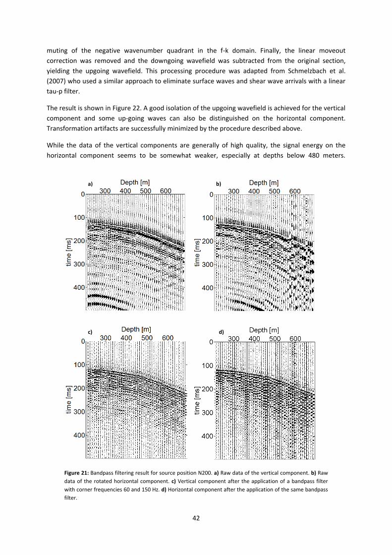
42

muting of the negative wavenumber quadrant in the f-k domain. Finally, the linear moveout correction was removed and the downgoing wavefield was subtracted from the original section, yielding the upgoing wavefield. This processing procedure was adapted from Schmelzbach et al. (2007) who used a similar approach to eliminate surface waves and shear wave arrivals with a linear tau-p filter.

The result is shown in Figure 22. A good isolation of the upgoing wavefield is achieved for the vertical component and some up-going waves can also be distinguished on the horizontal component. Transformation artifacts are successfully minimized by the procedure described above.

While the data of the vertical components are generally of high quality, the signal energy on the horizontal component seems to be somewhat weaker, especially at depths below 480 meters.

Figure 21: Bandpass filtering result for source position N200. a) Raw data of the vertical component. b) Raw data of the rotated horizontal component. c) Vertical component after the application of a bandpass filter with corner frequencies 60 and 150 Hz. d) Horizontal component after the application of the same bandpass filter.

a) b)

c) d)

43

5.3.2. Multicomponent Analysis In Figure 23, a possible processing flow for multicomponent VSP datasets is given that includes all the concepts that were discussed during this thesis. First, a single station polarization analysis could be conducted to rotate the horizontal components into the direction of the first arrivals. Additionally, a polarization filter can be applied to either enhance polarized events or suppress unwanted modes like tube waves. Then, the wavefield is separated into upgoing and downgoing waves. The downgoing wavefield can be put through a P- and S-wave separation algorithm like the controlled direction reception filter discussed in chapter 3. To do so, it suffices to use an approximate velocity function. This is possible, because the separation technique delivers reasonable results up to a velocity estimate error of about 30% (Greenhalgh et al., 1990). An accurate P- and S-wave velocity model for the migration can then be obtained by an analysis of the first arrival times on the separated P and S sections. These accurate velocity models are then fed into the migration algorithm together with the upgoing wavefield to obtain PP and PS migrated images.

a) b)

c) d)

Figure 22: Result of the wavefield separation into upgoing and downgoing waves for source position N200. a) Vertical component of the downgoing wavefield modeled by f-k filtering. b) Horizontal component of the downgoing wavefield. c) Vertical component of the upgoing wavefield obtained by subtracting a) from the original bandpass filtered vertical component section. d) Horizontal component of the upgoing wavefield.

44

Both the controlled direction reception algorithm for wavefield separation and the multicomponent migration routine were tested on the Benken dataset. The result of the P and S wavefield separation is shown in Figure 24 for source position S220. The algorithm was applied to the downgoing events only. The local P velocities around the receiver were taken from the Nagra report for the borehole in Benken (Nagra, 2001). They can be found in Appendix C. Unfortunately, no information about S velocities was available. Thus, a P to S velocity ratio (Vp/Vs) of 1.85 was assumed to calculate an approximate S velocity model. The separation appears to deliver reasonable results in the case of S-wave elimination (pass P waves). The first arrivals can clearly be identified as P-waves. Starting at a depth of approximately 440 meters, much P-wave energy appears to be leaking over into the S-wave section. This depth roughly corresponds to the top of the Dogger formation. Probably, the assumed P to S velocity ratio is not accurate enough for this formation. This impression is reinforced by the fact that very strongly dipping events (possible S-waves) can be observed in the original vertical component seismograms below this depth range. Above this critical depth, separated S-waves can be distinguished. To validate the reliability of the results, a synthetic dataset was created using finite difference modeling software. The input velocity model to the finite difference code is given in Appendix C. Unfortunately, the analysis of the modeled dataset did not provide any reliable information due to an error in the wavefield separation code that could not be identified and fixed before the end of this project. Still, at least a partial separation of the wavefield was achieved by the algorithm.

Figure 23: Suggested processing sequence for a multicomponent dataset

45

Finally, the vertical and the horizontal component data of the upgoing wavefield were fed into the multicomponent migration routine. The grid was limited to the vicinity of the borehole, ranging from 110 meters North to 75 meters South. The maximum investigated depth was 1000 meters. With a pixel size of 1x1 meters, this resulted in a total grid size of 185x1000 pixels. Using the source coordinates in Appendix B and the receiver depths, the vertical and horizontal distances from each source to each grid point and from each grid point to each receiver could be calculated. The computation was carried out on a Lenovo W520 laptop computer with an Intel Core i7-2760QM quadcore CPU and 8GB of RAM and took about 24 hours to run.

The result of the multicomponent migration is shown in Figure 25. The four plots are for a multicomponent PP-migration, a multicomponent PS-migration, a conventional PP migration of the vertical component and a PP migration of the horizontal component. At first glance, it appears that the results are somewhat over-migrated. The reason for this could be an erroneous velocity model or inaccurate raytracing.

a) b)

c) d)

Figure 24: Result of controlled direction reception filtering algorithm on the downgoing wavefield recorded from source position S220. a) Vertical component of the downgoing wavefield. b) Horizontal component of the downgoing wavefield. c) CDRII to pass P waves. d) CDRII to pass S waves.

46

An interesting fact is that the horizontal component and the vertical component PP migrations appear to complement each other quite nicely. Where the vertical component migration shows high amplitudes, the horizontal component migration does not, and vice versa. Still, the same features can be observed on both sections. This indicates that the horizontal component data quality is good enough to obtain accurate multicomponent migrations. Only small differences can be observed between the multicomponent PP migration and the vertical component migration. The slight mismatch between the sections can only be observed when they are overlain directly on top of each other. Here the multicomponent migration shows a little more detail towards the edges of the image. The multicomponent PS section appears to be somewhat lower in frequency than the others. Still, several events can be correlated between the PS and the PP section. Strong reflection events can be observed on the multicomponent PS section and partially on the multicomponent PP section at depths of approximately 500 m, 600 m, 650 m and 700 m. Further investigation and comparison with the 3D seismic data would be needed to ascertain if these events can be directly linked to the geological formations given in Appendix C. As mentioned before, it is possible that the results are impaired by an erroneous velocity model, inaccurate raytracing or static effects.

The results show that a further multicomponent investigation of the Benken dataset could be profitable. Some improvements to the algorithm that is presented in this thesis would probably be necessary. Possibilities to consider include the introduction of weighting terms to account for attenuation effects, and the implementation of a faster and more accurate raytracer that also can handle laterally varying velocities. Also, the algorithm could possibly be improved if the polarization would be calculated directly from the data (e.g., by a covariance eigenvalue analysis) instead of by raytracing through a possibly erroneous velocity model. Such an algorithm was suggested, for example, by Hou & Marfurt (2002).

a) b) c) d)

Figure 25: Result of the multicomponent migration. The black dots mark the receiver positions a) Multicomponent PP-migration b) Multicomponent PS migration c) Vertical component PP-migration d) Horizontal component PP-migration

47

6Chapter 6

Conclusions and Outlook In this thesis I presented the results of a theoretical and computational study on the potential of multicomponent (vector) seismic processing and analysis techniques for improved subsurface exploration. Synthetic and real data experiments were conducted to illustrate the advantages of vector wavefield processing compared to conventional scalar wavefield processing. The experiments were also designed to test the performance of the computer programs that were developed as part of this project. Good results were obtained for the synthetic data examples and most of the concepts could also be successfully applied to real data. In the following, the results of each of the proposed multicomponent processing techniques are individually discussed.

6.1. Conclusions It was shown that single triaxial station polarization filtering can be a powerful tool in the suppression of coherent and random noise. A single station polarization filter, based on singular value decomposition of the data within a specific time window enclosing the event of interest, could be successfully applied to a real surface recorded dataset. Although the data quality of the horizontal component record was rather poor, most of the elliptically polarized arrivals (Rayleigh waves) could be identified and removed from the data while the rectilinearly polarized reflection signal of interest remained in the section. This approach is of special interest for field sites where an equally sampled high density long aperture array cannot be laid out (e.g., in mines or VSP). Here, the method provides a viable alternative to conventional f-k or tau-p filtering.

The multi-station triaxial array polarization filter technique for wavefield separation, implemented in tau-p space, that was developed in this thesis performed well on synthetic data. There, not only a separation into P- and S-waves could be observed but also strong suppression of random noise was achieved. On the real dataset, the algorithm was at least partially successful. While the results of the P wave section looked reasonable, energy spill-over from the P-section into the S-section could be observed. The reason for this contamination is probably the choice of an erroneous P to S velocity ratio. The separated wavefields can provide high resolution time picks that can be used to obtain accurate P- and S-wave velocity models for the multicomponent migration, or they can be directly put through a scalar migration algorithm.

The multicomponent (polarization) migration of the Benken dataset indicated that the algorithm probably needs to be improved further before it is able to fully reconstruct the true geological setting. Still, it could be shown that a further multicomponent investigation of the dataset would be profitable. The data quality on the horizontal components seems to be good enough to obtain multicomponent migrations. In the PS migration map, strong reflectors can be observed. Further investigation would be needed to see if they can be linked to the known geological formations in the area.

Overall, the analysis yielded promising results for both synthetic and real data, indicating great potential benefits of multicomponent seismic processing compared to usual scalar wavefield

48

processing. Some of the major advantages are: successful ground roll suppression with short unequally sampled arrays, wavefield separation allowing high resolution time picks, better angular resolution in the migration maps and additional information on the geological target provided by shear waves (e.g., to study anisotropy).

6.2. Outlook Some of the algorithms that were discussed in this thesis could be further improved. This is particularly true for the multicomponent migration routine. Possible improvements could be made by the introduction of weighting terms to account for attenuation effects and by the implementation of an efficient and accurate raytracer that is also able to handle laterally varying velocity models. Also, the polarization properties could be directly determined from the data instead of by raytracing through a possibly erroneous medium.

Further investigations on the Benken dataset could involve wavefield separation tests with different Vp/Vs ratios in order to obtain more accurate representation of the P- and S-wavefields and a correlation of the multicomponent migration results with the local geology, borehole logs and the results of the 3D seismic investigation in the area. Finally, a migration using a modified version of the proposed migration routine could yield additional information about the seismic reflectors.

49

Bibliography Beylkin, G. (1987). Discrete Radon Transform. IEEE Transactions on Acoustics, Speech, and Signal Processing , 35 (2), 162-172.

Bohlen, T., DeNil, D., Köhn, D., & Jetschny, S. (2012). SOFI2D: seismic modeling with finite differences. 2D - elastic and viscoelastic version. Karlsruhe: Karlsruhe Institute of Technology.

Born, M., & Wolf, E. (1975). Principles of Optics. Oxford: Pergamon Press.

Cao, S., & Greenhalgh, S. (1994). Finite difference solution of the eikonal equation using an efficient, first-arrival wavefront tracking scheme. Geophysics , 59, 632-643.

Chang, W., & McMechan, G. (1994). 3-D elastic prestack, reverse-time depth migration. Geophysics , 59 (4), 597-609.

Cichowicz, A., Green, R., & Brink, A. (1988). Coda polarization properties of high frequency microseismic events. Bulletin of the Seismological Society of America , 78 (3), 1297-1318.

Claerbout, J. (1985). Imaging of the Earth's Interior. Oxford: Blackwell Scientific Publications.

Crampin, S. (1985). Evaluation of anisotropy by shear-wave splitting. Gephysics , 50 (1), 142-152.

Dankbaar, J. (1985). Separation of P- and S-Waves. Geophysical Prospecting , 33, 970-986.

Di Siena, J., Gaiser, J., & Corrigan, D. (1985). Horizontal components and shear wave analysis of three-component VSP data. London: Geophysical Press.

Esmersoy, C. (1984). Polarization analysis, orientation and velocity estimation in three-component VSP. In M. Tokosz, & R. Stewart, Vertical Seismic Profiling - Part B: Advanced Concepts (pp. 236-255). London: Geophysical Press.

Flinn, E. (1984). Signal analysis using rectilinearity and direction of particle motion. Proceedings of the IEEE , 53 (12), 1874-1876.

Foster, D., & Gaiser, J. (1986). Elastic Wave Field Decomposition of Offset VSP Data. SEG Annual Meeting (pp. 563-565). Houston, Texas: Society of Exploration Geophysicists.

Foster, D., & Mosher, C. (1992). Suppression of multiple reflections using the Radon transform. Geophysics , 57 (3), 386-395.

Franco, R., & Musacchio, G. (2001). Polarization filter with singular value decomposition. Geophysics , 66 (3), 932-938.

Friedlander, B. (2009). Wireless Direction Finding Fundamentals. In T. Tuncer, & B. Friedlander, Classical and Modern Direction-of-Arrival Estimation (pp. 1-51). Burlington: Academic Press.

Gal'perin, E. I. (1983). The Polarisation Method of Seismic Exploration. Dordrecht: Reidel Publishing.

Granli, J., Arntsen, B., & Sollid, A. H. (1999). Imaging through gas-filled sediments using marine shear-wave data. Geophysics , 64 (3), 668-677.

50

Greenhalgh, S. A., Zhou, B., & Rutty, M. (2008). Effect of coherent noise on single-station direction of arrival estimation. Journal of Seismology , 12 (3), pp. 377-385.

Greenhalgh, S. (2012). Single station triaxial seismic direction finding. Technical Note. ETH Zürich: Institute of Geophysics.

Greenhalgh, S., & King, D. (1981). Curved raypath interpretation of seismic refraction data. Geophysical Prospecting , 29, 853-882.

Greenhalgh, S., Mason, I., & Zhou, B. (2005). An analytical treatment of single station triaxial seismic direction finding. Journal of Geophysics and Engineering , 2, 8-15.

Greenhalgh, S., Mason, I., Lucas, E., Pant, D., & Eames, R. (1990). Controlled direction reception filtering of P- and S-waves  in  τ-p space. Geophysics Journal International , 100, 221-234.

Hearn, S., & Hendrick, N. (1999). A review of single station time-domain polarization analysis techniques. 8, 181-202.

Hinds, R., Anderson, N., & Kuzminski, R. (1996). VSP Interpretive Processing: Theory and Practice. Tulsa, Oklahoma: Society of Exploration Geophysicists.

Hokstad, K. (2000). Multicomponent Kirchhoff migration. Geophysics , 63, 1685-1695.

Hou, A., & Marfurt, K. (2002). Multicomponent prestack depth migration by scalar wavefield extrapolation. Geophysics , 67 (6), 1886-1894.

Jackson, G., Mason, I., & Greenhalgh, S. (1991). Principal component transforms of triaxial recordings by singular value decomposition. Geophysics , 56 (4), 528-533.

Jackson, G., Mason, I., & Lee, D. (1991). Multicomponent common-receiver gather migration of single-level walk away seismic profiles. Geophysical Prospecting , 39, 1015-1029.

Jepsen, D., & Kennet, B. (1990). Three component analysis of regional seismograms. Bulletin of the Seismological Society of America , 80 (6), 2032-2052.

Jin, S., & Shuki, R. (2005). Ground roll detection and attenuation by 3C polarization analysis. 67th Mtg: European Association of Geoscientists and Engineers (p. B020). Madrid: EAGE.

Kabir, M., & Marfurt, J. (1999). Toward true multiple removal. The Leading Edge , 18 (1), 66-73.

Kendall, R. (2005). An SVD-polarization Filter for Ground Roll Attenuation on Multicomponent Data. SEG Annual Meeting (pp. 65-75). Houston: Society of Exploration Geophysicists.

Kennet, B. (1991). The removal of free surface interactions from three-component seismograms. Geophysics Journal International , 104, 153-163.

Kuo, J., & Dai, T. (1984). Kirchhoff elastic wave migration for the case of noncoincident source and receiver. Geophysics , 49 (8), 1223-1238.

Magotra, N., Ahmend, N., & Chael, E. (1987). Seismic event detection and source location using single-station (three-component) data. Bulletin of the Seismological Society of America , 77 (3), 958-971.

51

Margrave, G. (2003). Numerical methods of exploration seismology. The University of Calgary: Department of Geology and Geophysics.

Montalbetti, J., & Kanasewich, E. (1970). Enhancement of teleseismic body phases with a polarization filter. Geophysical Journal of the Royal Astronomical Society , 21 (2), 119-129.

Nagra. (2001). Technischer Bericht 00-01: Sondierbohrung Benken. Untersuchungsbericht. Wettingen: Nagra.

Neidell, N., & Turhan Taner, M. (1971). Semblance and other coherency measures for multichannel data. Geophysics , 36 (3), 482-497.

Orlowsky, D., & Albert, W. (1999). Nagra. Interner Bericht 99-35. Sondierbohrung Benken: Walkaway VSP. Wettingen: Nagra.

Pugin, A., Pullan, S., & Hunter, J. (2009). Multicomponent high-resolution seismic reflection profiling. The Leading Edge , 1248-1261.

Russel, B., Hampson, D., & Chun, J. (1990). Noise elimination and the Radon transform. The Leading Edge , 9 (10), 18-3.

Rutty, M., & Greenhalgh, S. (1993). The correlation of seismic events on multicomponent data in the presence of coherent noise. Geophysics Journal International , 113, 343-385.

Schmelzbach, C., Horstmeyer, H., & Juhlin, C. (2007). Shallow 3D seismic-reflection imaging of fracture zones in crystalline rocks. Geophysics , 72 (6), B149-B160.

Schmidt, R. (1986). Multiple emitter location and signal parameter estimation. IEEE Transactions on Antennas and Propagation , 34 (3), 276-280.

Sinadinovski, C., Greenhalgh, S., & Mason, I. (1995). Three-dimensional reflector imaging of in-mine high frequency crosshole seismic data. Exploration Geophysics , 325-330.

Turner, G. (1990). Aliasing in the tau-p transform and the removal of spatially aliased coherent noise. Geophysics , 55 (11), 1496-1503.

Vidale, J. (1986). Complex polarization analysis of particle motion. Bulletin of the Seismological Society of America , 76 (5), 1393-1405.

Yilmaz, Ö. (2008). Seismic Data Analysis: Processing, Inversion, and Interpretatio of Seismic Data. Tulsa, Oklahoma: Society of Exploration Geophysicists.

Zhe, J., & Greenhalgh, S. (1997). Prestack multicomponent migration. Geophysics , 62 (2), 598-613.

Zhou,  B.,  &  Greenhalgh,  S.  (1994).  Linear  and  parabolic  τ-p transforms revisited. Geophysics , 59 (7), 1133-1149.

52

List of Figures Figure 1: Triaxial seismic direction finding problem (after Greenhalgh, Mason, & Zhou, 2005). 3 Figure 2: a) Synthetic triaxial record including two P-wave arrivals, corrupted by 50 percent of noise. b)

Result of the polarization analysis with the vector centroid method. The angle represents the azimuth and the distance from the center the inclination of arrival direction. 6

Figure 3: Analysis of a three-component record using a brute force grid search approach. The record contains two P-wave arrivals at 150 milliseconds (Ө:45,ф:45) and at 450 milliseconds (Ө:60,ф:10). a) Time slices taken at 150 milliseconds. b) Time slices taken at 450 milliseconds. c) Vertical cross-sections through the three-dimensional solution space, showing the evolution of the polarization properties over time. Results for the azimuth are displayed on the left and results for the inclination on the right. 9

Figure 4: Hodograms in the X-Y, X-Z and Y-Z planes representing the noise-free arrivals of a P- (Ө=70,ф=20), an SV- (Ө=70,ф=20) and a Rayleigh (Ө=45,ф=20) wave. 11

Figure 5: Power, cross-correlation and semblance in the X-Y plane for a P-wave arriving with an azimuth of 90 degrees. 12

Figure 6: Quantified error in the direction estimation caused by gain misalignments between the horizontal and the vertical channel. The gains are applied to the vertical channel only, unit gain is assumed for the horizontal channel. 14

Figure 7: a) Synthetic seismogram showing the arrival of a Rayleigh (200 ms) wave and a P-Wave (450 ms). b) Hodograms indicating the elliptical and rectilinear appearance of the two events. c) Measures of polarization built from the eigenvalues and eigenvectors of the complex covariance matrix. P1: Degree of polarization adapted from Esmersoy (1984) and Born & Wolf (1975), P2: Ellipticity of the signal, P3: Function to suppress elliptically polarized signals. 16

Figure 8: Horizontal components of a VSP shot gather before (top and middle) and after rotation into the direction of the first arrivals (bottom). 19

Figure 9: Ground roll attenuation achieved by a non-linear polarization filter using singular value decomposition. a) Input data of the vertical (Z) and horizontal (H1,H2) components. b) output of the polarization filter algorithm. 20

Figure 10: A seismic wave impinges on an array of two component receivers that are oriented in the sagittal plane. For P-waves, particle motion is parallel to the wave direction whereas for S-waves it is orthogonal to it. The local velocity around the receiver varies along the array (after Greenhalgh, 1990). 24

Figure 11: Processing steps for the P- and S-wavefield separation using controlled direction reception filtering of type 1 and 2 (after Greenhalgh et al. , 1990). 28

Figure 12: Wavefield separation using controlled direction reception filtering. Top panels: a) Vertical component and b) horizontal component of the original biaxial record. Middle panels: Result of the wavefield separation algorithm using a simultaneous rotation and Radon transform operator (CDRI) to pass c) P- or d) S-Waves. Bottom panels: Result of the wavefield separation after the application of a polarization gain function to boost rectilinearly polarized pixels in ω-p space (CDRII). e) Pass P-waves. f) Pass S-waves. 29

Figure 13: Pass and extinction planes for P- and S-waves in τ-p space. a) CDRI: P-wave pass plane. b) CDRI: S-wave pass plane. c) CDRI: P-wave extinction plane d) CDRI: S-wave extinction plane. e) CDRII: P-wave pass plane. f) CDRII: S-wave pass plane. 30

Figure 14: a) Vertical component of biaxial record corrupted by 70% of random noise. b) Horizontal component of the record with 50% of random noise. c) Output P-section of the wavefield separation algorithm. d) Output S-section of the wavefield separation algorithm. 31

Figure 15: The raytracing problem of the pre-stack Huygen's-Kirchhoff migration that was developed as part of this thesis. 34

53

Figure 16: Impulse response of three diffractors located at offsets and depths of (50m, 50m), (500m, 500m) and (950m, 50m) to a shot from the surface, located at offset 500 meters. 35

Figure 17: Kirchhoff migration result of a simple synthetic dataset collected over a homogeneous medium containing three point diffractors. Shown are the multicomponent P-P and P-S migration results as well as the results of scalar migrations of the horizontal and vertical component seismograms using the velocity of the P-wave (left) and a combined P- and S-wave velocity (right). 36

Figure 18: Input model to the finite difference code SOFI2D. On the left: P wave velocity model. On the right: Density model. The vertical red line represents the receiver array. 37

Figure 19: sĞƌƚŝĐĂů�ĂŶĚ�ŚŽƌŝnjŽŶƚĂů�ĐŽŵƉŽŶĞŶƚ�ƐĞŝƐŵŽŐƌĂŵƐ�ŽďƚĂŝŶĞĚ�ďLJ�ĨŝŶŝƚĞ�ĚŝĨĨĞƌĞŶĐĞ�ŵŽĚĞůŝŶŐ͘ 38 Figure 20: DŝŐƌĂƚĞĚ�WͲW�ƐĞĐƚŝŽŶ�ŽĨ�ƚŚĞ�ĚĂƚĂ�ŽďƚĂŝŶĞĚ�ďLJ�ĨŝŶŝƚĞ�ĚŝĨĨĞƌĞŶĐĞ�ŵŽĚĞůŝŶŐ͘ 38 Figure 21: Bandpass filtering result for source position N200. a) Raw data of the vertical component. b) Raw

data of the rotated horizontal component. c) Vertical component after the application of a bandpass filter with corner frequencies 60 and 150 Hz. d) Horizontal component after the application of the same bandpass filter. 42

Figure 22: Result of the wavefield separation into upgoing and downgoing waves for source position N200. a) Vertical component of the downgoing wavefield modeled by f-k filtering. b) Horizontal component of the downgoing wavefield. c) Vertical component of the upgoing wavefield obtained by subtracting a) from the original bandpass filtered vertical component section. d) Horizontal component of the upgoing wavefield. 43

Figure 23: Suggested processing sequence for a multicomponent dataset. 44 Figure 24: Result of controlled direction reception filtering algorithm on the downgoing wavefield recorded

from source position S220. a) Vertical component of the downgoing wavefield. b) Horizontal component of the downgoing wavefield. c) CDRII to pass P waves. d) CDRII to pass S waves. 45

Figure 25: Result of the multicomponent migration. The black dots mark the receiver positions a) Multicomponent PP-migration b) Multicomponent PS migration c) Vertical component PP-migration d) Horizontal component PP-migration. 46

54

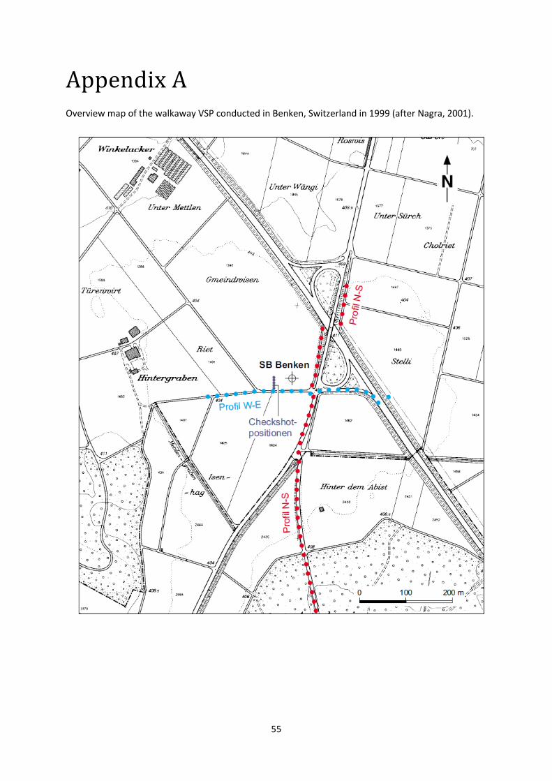
55

Appendix A Overview map of the walkaway VSP conducted in Benken, Switzerland in 1999 (after Nagra, 2001).

56

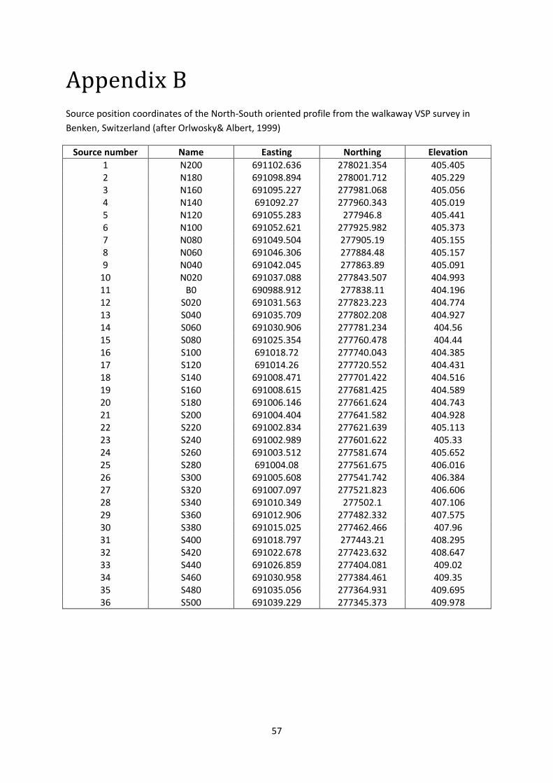
57

Appendix B Source position coordinates of the North-South oriented profile from the walkaway VSP survey in Benken, Switzerland (after Orlwosky& Albert, 1999)

Source number Name Easting Northing Elevation 1 N200 691102.636 278021.354 405.405 2 N180 691098.894 278001.712 405.229 3 N160 691095.227 277981.068 405.056 4 N140 691092.27 277960.343 405.019 5 N120 691055.283 277946.8 405.441 6 N100 691052.621 277925.982 405.373 7 N080 691049.504 277905.19 405.155 8 N060 691046.306 277884.48 405.157 9 N040 691042.045 277863.89 405.091

10 N020 691037.088 277843.507 404.993 11 B0 690988.912 277838.11 404.196 12 S020 691031.563 277823.223 404.774 13 S040 691035.709 277802.208 404.927 14 S060 691030.906 277781.234 404.56 15 S080 691025.354 277760.478 404.44 16 S100 691018.72 277740.043 404.385 17 S120 691014.26 277720.552 404.431 18 S140 691008.471 277701.422 404.516 19 S160 691008.615 277681.425 404.589 20 S180 691006.146 277661.624 404.743 21 S200 691004.404 277641.582 404.928 22 S220 691002.834 277621.639 405.113 23 S240 691002.989 277601.622 405.33 24 S260 691003.512 277581.674 405.652 25 S280 691004.08 277561.675 406.016 26 S300 691005.608 277541.742 406.384 27 S320 691007.097 277521.823 406.606 28 S340 691010.349 277502.1 407.106 29 S360 691012.906 277482.332 407.575 30 S380 691015.025 277462.466 407.96 31 S400 691018.797 277443.21 408.295 32 S420 691022.678 277423.632 408.647 33 S440 691026.859 277404.081 409.02 34 S460 691030.958 277384.461 409.35 35 S480 691035.056 277364.931 409.695 36 S500 691039.229 277345.373 409.978

58

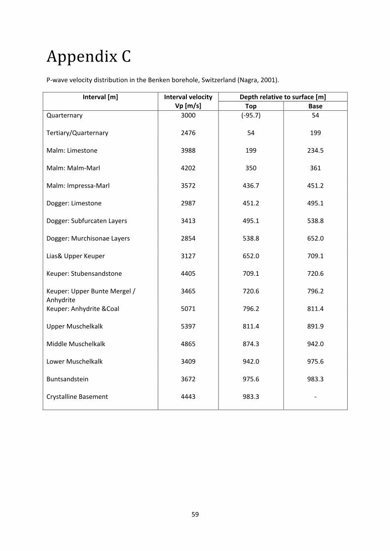
59

Appendix C P-wave velocity distribution in the Benken borehole, Switzerland (Nagra, 2001).

Interval [m] Interval velocity Vp [m/s]

Depth relative to surface [m] Top Base

Quarternary 3000 (-95.7) 54

Tertiary/Quarternary 2476 54 199

Malm: Limestone 3988 199 234.5

Malm: Malm-Marl 4202 350 361

Malm: Impressa-Marl 3572 436.7 451.2

Dogger: Limestone 2987 451.2 495.1

Dogger: Subfurcaten Layers 3413 495.1 538.8

Dogger: Murchisonae Layers 2854 538.8 652.0

Lias& Upper Keuper 3127 652.0 709.1

Keuper: Stubensandstone 4405 709.1 720.6

Keuper: Upper Bunte Mergel / Anhydrite

3465 720.6 796.2

Keuper: Anhydrite &Coal 5071 796.2 811.4

Upper Muschelkalk 5397 811.4 891.9

Middle Muschelkalk 4865 874.3 942.0

Lower Muschelkalk 3409 942.0 975.6

Buntsandstein 3672 975.6 983.3

Crystalline Basement 4443 983.3 -

60

61

Acknowledgements I would like to express my deep gratitude to my supervisors Stewart Greenhalgh and Cedric Schmelzbach. They were always available for my questions and patiently helped me overcome many difficulties in the production of this thesis. In various inspiring discussions they broadened my horizon in the field of seismic processing. Without their dedicated assistance, this work would not have been possible.

I would like to thank my colleagues in the programme for their willingness to help me out whenever I encountered a problem and for all the good moments we spent together.

I also wish to thank my family for their continuous support during this project and the semesters I spent abroad.

Finally, I would like to thank Kathrin for balancing my life besides the thesis and for standing all my moods.

62