Embed Size (px)
Citation preview

Chapter 9
Multicollinearity
9.1 The Nature of Multicollinearity
9.1.1 Extreme Collinearity
The standard OLS assumption that (xi1, xi2, . . . , xik ) not be linearly relatedmeans that for any ( c1, c2, . . . , ck )
xik 6= c1xi1 + c2xi2 + · · ·+ ck−1xi,k−1 (9.1)
for some i. If the assumption is violated, then we can find ( c1, c2, . . . , ck−1 )such that
xik = c1xi1 + c2xi2 + · · ·+ ck−1xi,k−1 (9.2)
for all i. Define
X1 =
⎛⎜⎜⎜⎝x12 · · · x1kx22 · · · x2k...
...xn2 · · · xnk
⎞⎟⎟⎟⎠ , xk =
⎛⎜⎜⎜⎝xk1xk2...
xkn
⎞⎟⎟⎟⎠ , and c =
⎛⎜⎜⎜⎝c1c2...
ck−1
⎞⎟⎟⎟⎠ .
Then extreme collinearity can be represented as
xk = X1c. (9.3)
We have represented extreme collinearity in terms of the last explanatory vari-able. Since we can always re-order the variables this choice is without loss ofgenerality and the analysis could be applied to any non-constant variable bymoving it to the last column.
104

9.1. THE NATURE OF MULTICOLLINEARITY 105
9.1.2 Near Extreme Collinearity
Of course, it is rare, in practice, that an exact linear relationship holds. Instead,we have
xik = c1xi1 + c2xi2 + · · ·+ ck−1xi,k−1 + vi (9.4)
or, more compactly,
xk = X1c+ v, (9.5)
where the v’s are small relative to the x’s. If we think of the v’s as randomvariables they will have small variance (and zero mean if X includes a columnof ones).A convenient way to algebraically express the degree of collinearity is the
sample correlation between xik and wi = c1xi1+c2xi2+· · ·+ck−1xi,k−1, namely
rx,w =cov(xik, wi )pvar(xi,k) var(wi)
=cov(wi + vi, wi )pvar(wi + vi) var(wi)
(9.6)
Clearly, as the variance of vi grows small, this value will go to unity. For nearextreme collinearity, we are talking about a high correlation between at leastone variable and some linear combination of the others.We are interested not only in the possibility of high correlation between xik
and the linear combination wi = c1xi1+ c2xi2+ · · ·+ ck−1xi,k−1 for a particularchoice of c but for any choice of the coefficient. The choice which will maximizethe correlation is the choice which minimizes
Pni=1w
2i or least squares. Thusbc = (X0
1X1)−1X0
1xk and bw = X1bc and(rxk,w)
2 = R2k· (9.7)
is the R2 of this regression and hence the maximal correlation between xki andthe other x’s.
9.1.3 Absence of Collinearity
At the other extreme, suppose
R2k· = rxk,w = cov(xik, bwi ) = 0. (9.8)
That is, xik has zero correlation with all linear combinations of the other vari-ables for any ordering of the variables. In terms of the matrices, this requiresbc = 0 or
X01xk = 0. (9.9)
regardless of which variable is used as xk. This is called the case of orthogonalregressors, since the various x’s are all orthogonal. This extreme is also veryrare, in practice. We usually find some degree of collinearity, though not perfect,in any data set.

106 CHAPTER 9. MULTICOLLINEARITY
9.2 Consequences of Multicollinearity
9.2.1 For OLS Estimation
We will first examine the effect of xk1 being highly collinear upon the estimatebβk. Now letxk = X1c+ v (9.10)
The OLS estimates are given by the solution of
X0y = X0Xbβ= X0(X1 : xk )bβ= (X0X1 : X
0xk )bβ (9.11)
Applying Cramer’s rule to obtain bβk yieldsbβk = |X0X1 : X
0y||X0X| (9.12)
However, as the collinearity becomes more extreme, the columns of X (the rowsof X0) become more linearly dependent and
limv→0
bβ1 = 0
0(9.13)
which is indeterminant.Now, the variance-covariance matrix is
σ2(X0X )−1 = σ21
|X0X| adj(X0X )
= σ21
|X0X| adj∙µ
X01
x0k
¶(X1 : xk )
¸= σ2
1
|X0X| adjµX01X1 X0
1xkX01xk x0kxk
¶. (9.14)
The variance of bβk is given by the (k, k) element, sovar( bβk ) = σ2
1
|X0X| cof(k, k) = σ21
|X0X| |X01X1|. (9.15)
Thus, for |X01X1| 6= 0, we have
limv→0
var( bβk ) = σ2|X01X1|0
=∞. (9.16)
and the variance of the collinear terms becomes unbounded.

9.2. CONSEQUENCES OF MULTICOLLINEARITY 107
It is instructive to give more structure to the variance of the last coefficientestimate in terms of the sample correlation R2k· given above. First we obtain thecovariance of the OLS estimators other than the intercept. DenoteX = ( : X∗)where is an n × 1 vector of ones and X∗ are the nonconstant columns of X,then
X0X =
∙ 0 0X∗
X∗0 X∗0X∗
¸. (9.17)
Using the results for the inverse of a partitioned matrix we find that the lowerright-hand k − 1× k − 1 submatrix of the inverse is given by
(X∗0X∗ −X∗0 ( 0 )−1 0X∗)−1 = (X∗0X∗ − nx∗x∗0)−1
= [(X∗ − x∗0)0(X∗ − x∗0)]−1
= (X0X)−1
where x∗ = 0X∗/n is the mean vector for the nonconstant variables andX = X∗ − x∗0 is the demeaned or deviation form of the data matrix for thenonconstant variables.We now denote X = (X1 : xk) where xk is last column (k − 1)th, then
X0X =
∙X01X1 X
0xk
x0kX x0kxk
¸. (9.18)
Using the results for partitioned inverses again, the (k, k) element of the inverse
of (X0X)−1 is given by,
(x0kxk − x0kX1(X01X1)
−1X01xk)
−1 = 1/(x0kxk − x0kX1(X01X1)
−1X01xk)
= 1/e0kek
= 1/(x0kxk · e0kek/x0kxk)
= 1/(x0kxk(1−SSEk
SSTk))
= 1/(x0kxk(1−R2k·))
where ek = (In − X1(X01X1)
−1X01)xk are the OLS residuals from regressing
the demeaned xk’s on the other variables and SSEk, SSTk, and R2k· are thecorresponding statistics for this regression. Thus we find
var(bβk) = σ2[(X0X )−1]kk = σ2/(x0kxk(1−R2k·)) (9.19)
= σ2/(Pn
i=1(xik − xk)2(1−R2k·))
= σ2/(n · 1n
Pni=1(xik − xk)
2(1−R2k·)).
and the variance of bβk increases with the noise σ2 and the correlation R2k· of xkwith the other variables, and decreases with the sample size n and the signal

108 CHAPTER 9. MULTICOLLINEARITY
1n
Pni=1(xik−xk)2. Since the order of the variables is arbitrary and any could be
placed in the k-th position, var(bβj) will be the same expression with j replacingk.Thus, as the collinearity becomes more and more extreme:
• The OLS estimates of the coefficients on the collinear terms become in-determinant. This is just a manifestation of the difficulties in obtaining(X0X)−1.
• The OLS coefficients on the collinear terms become infinitely variable.Their variances become very large as R2k· → 1.
• The OLS estimates are still BLUE and with normal disturbances BUE.Thus, any unbiased estimator will be afflicted with the same problems.
Collinearity does not effect our estimate s2 of σ2. This is easy to see, sincewe have shown that
(n− k )s2
σ2∼ χ2n−k (9.20)
regardless of the values of X, provided X0X still nonsingular. This is to becontrasted with the bβ where
bβ ∼ N(β, σ2(X0X )−1 ) (9.21)
clearly depends on X and more particularly the near non-invertibility of X0X.
9.2.2 For Inferences
Provided collinearity does not become extreme, we still have the ratios (bβj −βj)/√s2djj ∼ tn−k where d
jj = [(X0X )−1]jj . Although bβj becomes highlyvariable as collinearity increases, djj grows correspondingly larger, thereby com-pensating. Thus under H0 : βj = β0j , we find (
bβj − β0j )/√s2djj ∼ tn−k, as is
the case in the absence of collinearity. This result that the null distribution ofthe ratios is not impacted as collinearity becomes more extreme seems not tobe fully appreciated in most texts.The inferential price extracted by collinearity is loss of power. Under H0 :
βj = β1j 6= β0j , we can write
(bβj − β0j )/√s2djj = (bβj − β1j )/
√s2djj + (β1j − β0j )/
√s2djj .
(9.22)
The first term will continue to follow a tn−k distribution, as argued in theprevious paragraph, as collinearity becomes more extreme. However, the secondterm, which represents a “shift” term, will grow smaller as collinearity becomes

9.2. CONSEQUENCES OF MULTICOLLINEARITY 109
more extreme and djj becomes larger. Thus we are less likely to shift thestatistic into the tail of the ostensible null distribution and hence less likely toreject the null hypothesis. Formally, (bβj − β0j )/
√s2djj will have a noncentral t
distribution, but the noncentrality parameter will become smaller and smalleras collinearity becomes more extreme.Alternatively the inferential impact can be seen through the impact on the
confidence intervals. Using the standard approach discussed in the previouschapter, we have [bβj − a
√s2djj , bβj + a
√s2djj) as the 95% confidence interval,
where a is the critical value for a .025 tail. Note that as collinearity becomesmore extreme and djj becomes larger, the width of the interval becomes largeras well. Thus we see that the estimates are consistent with a larger and largerset of null hypothesis as the collinearity strengthens. In the limit it is consistentwith any null hypothesis and we have zero power.We should emphasize that collinearity does not always cause problems. The
shift term in (9.xx) can be written
(β1j − β0j )/√s2djj =
√n(β1j − β0j )/
rσ2/(
1
n
Pni=1(xik − xk)2(1−R2j·))
which clearly depends on other factors than the degree of collinearity. The sizeof the shift increases with the sample size
√n, the difference between the null
and alternative hypotheses (β1j − β0j ), and the signal noise ratio (1n
Pni=1(xij −
xj)2/σ2. The important question is not whether collinearity is present or
extreme but whether is is extreme enought to eliminate the power of our test.This is also a phenonmenon that does not seem to be fully appreciated or well-enough advertised in most texts.We can easily tell when collinearity is not a problem if the coefficients are sig-
nificant or we reject the null hypothesis under consideration. Only if apparentlyimportant variables are insignificantly different from zero or have the wrong signshould we consider the possibility that collinearity is causing problems.
9.2.3 For Prediction
If all we are interested in is prediction of yp given xp1, xp2, . . . , xpk, then we arenot particularly interested in whether or not we have isolated the individualeffects of each xij . We are interested in predicting the total effect or variationin y.A good measure of how well the linear relationship captures the total effect
or variation is the R2 statistic. But the R2 value is related to s2 by
R2 = 1− e0e
(y − y)0(y − y)= 1− (n− k)
s2
var(y), (9.23)
which does not depend upon the collinearity of X.

110 CHAPTER 9. MULTICOLLINEARITY
Thus, we can expect our regressions to predict well, despite collinearity andinsignificant coefficients, provided the R2 value is high. This depends, of course,upon the collinearity continuing to persist in the future. If the collinearitydoes not continue, then prediction will become increasingly uncertain. Suchuncertainty will be reflected, however, by the estimated standard errors of theforcast and hence wider forecast intervals.
9.2.4 An Illustrative Example
As an illustration of the problems introduced by collinearity, consider the con-sumption equation
Ct = β0 + β1Yt + β2Wt + ut, (9.24)
where Ct is consumption expenditures at time t, Yt is income at time t and Wt
is wealth at time t. Economic theory suggests that the coefficient on incomeshould be slightly less than one and the coefficient on wealth should be positive.The time-series data for this relationship are given in the following table:
Ct Yt Wt
70 80 81065 100 100990 120 127395 140 1425110 160 1633115 180 1876120 200 2052140 220 2201155 240 2435150 260 2686
Table 9.1: Consumption Data
Applying least squares to this equation and data yields
Ct = 24.775(6.752)
+ 0.942(0.823)
Yt − 0.042(0.081)
Wt + et,
where estimated standard errors are given in parenthesis. Summary statisticsfor the regression are: SSE = 324.446, s2 = 46.35, and R2 = 0.9635. Thecoefficient estimate for the marginal propensity to consume seems to be a rea-sonable value however it is not significantly different from either zero or one.And the coefficient on wealth is negative, which is not consistent with economictheory. Wrong signs and insignificant coefficient estimates on a priori impor-tant variables are the classic symptoms of collinearity. As an indicator of thepossible collinearity the squared correlation between Yt and Wt is .9979, whichsuggests near extreme collinearity among the explanatory variables.

9.3. DETECTING MULTICOLLINEARITY 111
9.3 Detecting Multicollinearity
9.3.1 When Is Multicollinearity a Problem?
Suppose the regression yields significant coefficients, then collinearity is not aproblem–even if present. On the other hand, if a regression has insignificantcoefficients, then this may be due to collinearity or that the variables, in fact,do not enter the relationship.
9.3.2 Zero-Order Correlations
If we have a trivariate relationship, say
yt = β1 + β2xt2 + β3xt3 + ut, (9.25)
we can look at the zero-order correlation between x2 and x3. As a rule of thumb,if this (squared) value exceeds the R2 of the original regression, then we have aproblem of collinearity. If r23 is low, then the regression is likely insignificant.In the previous example, r2WY = 0.9979, which indicates that Yt is more
highly related to Wt than Ct and we have a problem. In effect, the variablesare so closely related that the regression has difficulty untangling the separateeffects of Yt and Wt.In general (k > 3), when one of the zero-order correlations between x0s is
large relative to R2 we have a problem.
9.3.3 Partial Regressions
In the general case (k > 3), even if all the zero-order correlations are small, wemay still have a problem. For while x1 my not be strongly linearly related to anysingle xi (i 6= 1), it may be very highly correlated with some linear combinationof xs.To test for this possibility, we should run regressions of each xi on all the
other xs. If collinearity is present, then one of these regressions will have a highR2 (relative to R2 for the complete regression).For example, when k = 4 and
yt = β1 + β2xt2 + β3xt3 + β4xt4 + ut (9.26)
is the regression, then collinearity is indicated when one of the partial regressions
xt2 = α1 + α3xt3 + α4xt4
xt3 = γ1 + γ2xt2 + γ4xt4 (9.27)
xt4 = δ1 + δ2xt2 + δ3xt3 (9.28)
yields a large R2 relative to the complete regression.

112 CHAPTER 9. MULTICOLLINEARITY
9.3.4 The F Test
The manifestation of collinearity is that estimators become insignificantly dif-ferent from zero, due to the inability to untangle the separate effects of thecollinear variables. If the insignificance is due to collinearity, the total effect isnot confused, as evidenced by the fact that s2 is unaffected.A formal test, accordingly, is to examine whether the total effect of the
insignificant (possibly collinear) variables is significant. Thus, we perform an Ftest to test the joint hypothesis that the individually insignificant variables areall insignificant.For example, if the regression
yt = β1 + β2xt2 + β3xt3 + β4xt4 + ut (9.29)
yields insignificant (from zero) estimates of β2, β3 and β4, we use an F testof the joint hypothesis β2 = β3 = β4 = 0. If we reject this joint hypothesis,then the total effect is strong, but the individual effects are confused. This isevidence of collinearity. If we accept the null, then we are forced to concludethat the variables are, in fact, insignificant.For the consumption example considered above, a test of the null hypothesis
that the collinear terms (income and wealth) are jointly zero yields an F -statisticvalue of 92.40 which is very extreme under the null when the variable has anF2,7. Thus the variables are individually insignificant but are jointly significant,which indicates that collinearity is, in fact, a problem.
9.3.5 The Condition Number
Belsley, Kuh, and Welsh (1980), suggest an approach that considers the invert-ibility of X directly. First, we transform each column of X so that they are ofsimilar scale in terms of variability by dividing each column to unit length:
x∗j = xj/qx0jxj (9.30)
for j = 1, 2, ..., k. Next we find the eigenvalues of the moment matrix of theso-transformed data matrix by finding the k roots of :
det(X∗0X∗ − λIk) = 0. (9.31)
Note that since X∗0X∗ is positive semi-difinite the eigenvalues will be betweenzero and one with values of zero in the event of singularity and close to zero inthe event of close to singularity. The condition number of the matrix is takenas the ratio of the largest to smallest of the eigenvalues:
c =λmaxλmin
. (9.32)

9.4. CORRECTING FOR COLLINEARITY 113
Using an analyis of a number of problems BKW suggest that collinearity is apossible issue when c ≥ 20. For the example the condition number is 166.245,which indicates a very poorly conditioned matrix. Although this approachtells a great deal about the invertibility of X0X and hence the signal, it tells usnothing about the noise level relative to the signal.
9.4 Correcting For Collinearity
9.4.1 Additional Observations
Professor Goldberger has quite aptly described multicollinearity as ”micronu-merosity” or not enough observations. Recall that the shift term depends onthe difference between the null and alternative, the signal-noise ratio, and thesample size. For a given signal-noise ratio, unless collinearity is extreme, itcan always be overcome by increasing the sample size sufficiently. Moreover, wecan sometimes gather more data that, hopefully, will not suffer the collinearityproblem. With designed experiments, and cross-sections, this is particularly thecase. With time series data this is not feasible and in any event gathering moredata is time-consuming and expensive.
9.4.2 Independent Estimation
Sometimes we can obtain outside estimates. For example, in the Ando-Modiglianiconsumption equation
Ct = β0 + β1Yt + β2Wt + ut, (9.33)
we might have a cross-sectional estimate of β1, say bβ1. Then,(Ct − bβ1Yt) = β0 + β2Wt + ut (9.34)
becomes the new problem. Treating bβ1 as known allows estimation of β2 withincreases in precision. It would not reduce the precision of the estimate of β1which would simply be the cross-sectional estimate. The implied error term,moreover, is more complicated since bβ1 may be correlated with Wt. Mixedestimation approaches should be used to handle this approach carefully. Notethat this is another way to gather more data.
9.4.3 Prior Restrictions
Consider the consumption equation from Klein’s Model I:
Ct = β0 + β1Pt + β2Pt−1β3Wt + β4W0t + ut, (9.35)

114 CHAPTER 9. MULTICOLLINEARITY
where Ct is the consumption expenditure, Pt is profits, Wt is the private wagebill and W 0
t is the governement wage bill.Due to market forces, Wt andW
0t will probably move together and collinear-
ity will be a problem for β3 and β4. However, there is no prior reason todiscriminate between Wt and W 0
t in their effect on Ct. Thus it is reasonable tosuppose Wt and W 0
t impact Ct in the same way. That is, β3 = β4. The modelis now
Ct = β0 + β1Pt + β2Pt−1β(Wt +W 0t) + ut, (9.36)
which should avoid the collinearity problem.
9.4.4 Ridge Regression
One manifestation of collinearity is that the effected estimates, say bβ1, will beextreme with a high probability. Thus,
kXi=1
bβ2i = bβ21 + bβ22 + · · ·+ bβ2k = bβ0bβ (9.37)
will be large with a high probability.By way of treating the disease by treating its symptoms, we might restrictbβ0bβ to be small. Thus, we might reasonably
minβ(y −Xbβ )0(y−Xbβ ) subject to bβ0bβ ≤ m. (9.38)
Form the Lagrangian (since bβ0bβ is large, we must impose the restriction withequality).
L = (y −Xeβ )0(y−Xeβ ) + λ(m− eβ0eβ )=
nXt=1
Ãyt −
kXi=1
eβixti!2 ++λ(m− kXi=1
eβ2i ). (9.39)
The first-order conditions yield
∂L∂βj
= −2Xt
Ãyt −
Xi
eβixti!xtj + 2λeβ2i = 0, (9.40)
or Xt
ytxtj =Xt
Xi
xtixtj eβi + λeβj=
Xi
eβiXt
xtixtj + λeβj , (9.41)

9.4. CORRECTING FOR COLLINEARITY 115
for j = 1, 2, . . . , k. In matrix form, we have
X0y = (X0X+ λIn)eβ. (9.42)
So, we have eβ = (X0X+ λIn)−1X0y. (9.43)
This is called ridge regression.Substition yieldseβ = (X0X+ λIn)
−1X0y
= (X0X+ λIn)−1X0(Xβ + u)
= (X0X+ λIn)−1X0(Xβ + (X0X+ λIn)
−1u) (9.44)
and
E( eβ ) = (X0X+ λIn)−1X0Xβ = Pβ, (9.45)
so ridge regression is biased. Rather obviously, as λ grows large, the expectation”shrinks” towards zero so the bias is towards zero. Next, we find that
Cov( eβ ) = σ2(X0X+ λIn)−1X0X(X0X+ λIn)
−1 = σ2Q < σ2(X0X)−1.(9.46)
If u ∼ N(0, σ2In), then eβ ∼ N(Pβ, σ2Q) (9.47)
and inferences are possible only for Pβ and hence the complete vector.The rather obvious question in using ridge regression is what is the best
choice for λ? We seek to trade off the increased bias against the reduction inthe variance. This may be done by considering the mean square error (MSE)which is given by
MSE(eβ) = σ2Q+ (P− Ik)ββ0(P− Ik)= (X0X+ λIn)
−1σ2X0X+ λ2ββ0(X0X+ λIn)−1.
We might choose to minimize the determinant or trace of this function. Notethat either is an decreasing function of λ through the inverses and an increasingfunction through the term in brackets. Note also that the minimand dependson the true unkown β, which makes it infeasible.In practice, it is useful to obtain what is called a ridge trace, which plots
out the estimates, estimated standard error, and estimated square root of meansquared error (SMSE) as a function of λ. Problematic terms will frequentlydisplay a change of sign and a dramatic reduction in the SMSE. If this phe-nonmenon occurs at a sufficiently small value of λ, then the bias will be smalland inflation in SMSE relative to the standard error will be small and we canconduct inference in something like the usual fashion. In particular, if theestimate of a particular coefficient seems to be significantly different from zerodespite the bias toward zero, we can reject the null that it is zero.

Chapter 10
Stochastic ExplanatoryVariables
10.1 Nature of Stochastic X
In previous chapters, we made the assumption that the x’s are nonstochastic,which means they are not random variables. This assumption was motivatedby the control variables in controlled experiments, where we can choose thevalues of the independent variables. Such a restriction allows us to focus onthe role of the disturbances in the process and was most useful in working outthe stochastic properties of the estimators and other statistics. Unfortunately,economic data do not usually come to us in this form. In fact, the independentvariables are typically random variables much like the dependent variable whosevalues are beyond the control of the researcher.Consequently we will restate our model and assumptions with an eye toward
stochastic x. The model is
yi = x0iβ + ui for i = 1, 2, ..., n. (10.1)
The assumptions with respect to unconditional moments of the disturbances arethe same as before:
(i) E[ui] = 0
(ii) E[u2i ] = σ2
(iii) E[uiuj ] = 0, j 6= i
The assumptions with respect to x must be modified. We replace the as-sumption of x nonstochastic with an assumption regarding the joint stochasticbehavior of ui and xi, which are taken to be jointly i.i.d.. Several alternative
116

10.1. NATURE OF STOCHASTIC X 117
assumptions will be introduced regarding the degree of dependence between xiand ui. For stochastic x, the assumption of linearly independent x’s impliesthat the covariance matrix of the x’s has full column rank and is hence positivedefinite. Stated formally, we have:
(iv) (ui,xi) jointly i.i.d. with dependence assumption
(v) E[xix0i] = Q p.d.
Notice that the assumption of normality, which was introduced in previouschapters to facilitate inference, was not reintroduced. Thus we are effectivelyrelaxing both the nonstochastic regressor and normality assumptions at thesame time. The motivation for dispensing with the normality assumption willbecome apparent presently.We will now examine the various alternative assumptions that will be enter-
tained with respect to the degree of dependence between xi and ui.
10.1.1 Independent X
The strongest assumption we can make relative to this relationship is that xiare stochastically independent of ui, so assumption (iv) becomes
(iv,a) (ui,xi) jointly i.i.d. with ui independent of xi.
This means that the distribution of xi depends in no way on the value of ui andvisa versa. Note that
cov ( g(xi), h(ui) ) = 0, (10.2)
for any functions g(·) and h(·), in this case.
10.1.2 Conditional Zero Mean
The next strongest assumption is E[ui|xi] = 0, so Assumption (iv) becomes
(iv,b) (ui,xi) jointly i.i.d. with E[ui|xi] = 0, E[u2i |xi] = σ2.
Note that this assumption implies
cov ( g(xi), ui) ) = 0, (10.3)
for any function g(·). This assumption is motivated by supposing that our modelis simply a statement of conditional expectation, E[yi|xi] = x0iβ, and some-times will not be accompanied by the conditional second moment assumption
E[u2i |xi] = σ2. Note that independence along with the unconditional statements
E[ui] = 0 and E[u2i ] = σ2 imply conditional zero mean and constant conditional
variance but not the reverse.

118 CHAPTER 10. STOCHASTIC EXPLANATORY VARIABLES
10.1.3 Uncorrelated X
A weaker assumption is that xij and ui are only uncorrelated, so Assumption(iv) becomes
(iv,c) (ui,xi) jointly i.i.d. with E[xiui] = 0.
This assumption only implies zero covariance in the levels of xi and ui, or forone element of xi,
cov (xij , ui ) = 0. (10.4)
The properties of bβ are less accessible in this case. Note that conditional zeromean always implies uncorrelated, but not the reverse. It is possible to havea random variables that are uncorrelated but neither has constant conditionalmean given the other. In general, the conditional second moment will also benonconstant. Note that conditional zero mean implies unconditional zero meanbut not the reverse.
10.1.4 Correlated X
A priori information sometimes suggests the possibility that xij is correlatedwith ui, so Assumption (iv) becomes
(iv,d) (ui,xi) jointly i.i.d. with E[xiui] = d, d 6= 0.
Stated another way
E(xij , ui ) 6= 0. (10.5)
for some j. As we shall see below, this can have quite serious implications forthe OLS estimates.An example is the case of simultaneous equations models that we will ex-
amine later in this chapter. A second example occurs when our right-hand sidevariables are measured with error. Suppose
yi = α+ βxi + ui (10.6)
is the true model but
x∗i = xi + vi (10.7)
is the only available measurement of xi. If we use x∗i in our regression, then we
are estimating the model
yi = α+ β(x∗i − vi ) + ui
= α+ βx∗i + (ui − βvi ). (10.8)
Now, even if the measurement error vi were independent of the disturbance ui,the right-hand side variable x∗t will be correlated with the effective disturbance(ui − βvi).

10.2. CONSEQUENCES OF STOCHASTIC X 119
10.2 Consequences of Stochastic X
10.2.1 Consequences for OLS Estimation
Recall that
bβ = (X0X )−1X0y (10.9)
= (X0X )−1XX 0(Xβ + u )
= β + (X0X )−1X0u
= β + (1
nX0X )−1
1
nX0u
= β +
Ã1
n
nPj=1
xjx0j
!−1µ1
n
nPi=1xiui
¶We will now examine the bias and consistency properties of the estimators underthe alternative dependence assumptions.
Uncorrelated X
Suppose, under Assumption (iv,c), that xt is only assured of being uncorrelatedwith ui. Rewrite the second term in (10.9) asÃ
1
n
nPj=1
xjx0j
!−1µ1
n
nPi=1xiui
¶=
1
n
nPi=1
⎡⎣Ã 1n
nPj=1
xjx0j
!−1xi
⎤⎦ui=
1
n
nPi=1
wiui.
Note that wi is a function of both xi and xj and is nonlinear in xi for j = i.Now ui is uncorrelated with the xj for j 6= i by independence and the levelof xi by the assumption but is not necessarily uncorrelated with the nonlinearfunction of xi. Thus, if the expectation exists,
E[(X0X )−1X0u] 6= 0, (10.10)
in general, whereupon
E[bβ] = β +E£(X0X )−1X0u
¤6= β. (10.11)
Similarly, we find E[s2] 6= σ2. Thus both bβ and s2 will be biased, although thebias may disappear asymptotically as we will see below. Note that sometimesthese expectations are not well defined.Now, each element of xix
0i and xiui are i.i.d. random variables with ex-
pectations Q and 0, respectively. Thus, the law of large numbers guarantees

120 CHAPTER 10. STOCHASTIC EXPLANATORY VARIABLES
that
1
n
nPi=1xixi −→p Exixi = Q, (10.12)
and
1
n
nPi=1xiui −→p Exiui = 0. (10.13)
It follows that
plimn→∞
bβ = β + plimn→∞
"µ1
nX0X
¶−11
nX0u
#
= β + plimn→∞
µ1
nX0X
¶−1plimn→∞
1
nX0u
= β +Q−1 · 0 = β. (10.14)
Similarly, we can show that
plimn→∞
s2 = σ2. (10.15)
Thus both bβ and s2 will be consistent.
Conditional Zero Mean
Suppose Assumption (iv,b) is satisfied, then E[ui|xi] = 0 and, by independenceacross i, we have E(u|X) = 0. It follows that
E[bβ] = β+E[(X0X)−1X0u]
= β+E[(X0X)−1X0
E(u|X)]= β+E[(X
0X)−1X0 · 0] = β.
and OLS is unbiased. Since conditional zero mean implies uncorrelatedness,then we have the same consistency results as before, namely
plimn→∞
bβ = β and plimn→∞
s2 = σ2. (10.16)
Suppose, further, that E[u2i |xi] = σ2 and hence E(uu0|X) = σ2In. Thenthe Gauss-Markov theorem continues to hold in the sense that least-squares isBLUE, given X, in the class of estimators that is linear in y with the lineartransformation matrix a function only of X. Under this conditional covariance

10.2. CONSEQUENCES OF STOCHASTIC X 121
assumption, we can show unbiasedness, in a similar fashion, for the varianceestimator,
E s2 = E e
0e/(n− k)
=1
n− kEu
0( In −X(X0X)−1X0 )u
= σ2. (10.17)
This estimator, being quadratic in u, and hence y, can be shown to be the bestquadratic unbiased estimator BQUE of σ2.
Independent X
Suppose Assumption (iv,a) holds, then xi is independent of ui. Since (i) and(ii) assure that E[ui] = 0 and E[u2i ] = σ2, we have conditional zero mean andconstant conditional variance and the corresponding unbiasedness results
E bβ = β and E s2 = σ2, (10.18)
together with the BLUE property and the consistency results
plimn→∞
bβ = β and plimn→∞
s2 = σ2. (10.19)
Correlated X
Finally, suppose Assumption (iv,d) applies, so xi is correlated with ui.and
Exiui = d 6= 0. (10.20)
Obviously, since xi is correlated with ui there is no reason to believe
E[(X0X )−1X0u] = 0 so the OLS estimator will be biased. Moreover, thisbias will not disappear in large samples as we will see below. Turning to thepossibility of consistency, we see, by the law of large numbers that
1
n
nPi=1xiui
p−→ Exiui = d, (10.21)
whereupon
plimn→∞
bβ = β +Q−1 · d 6= β (10.22)
since Q−1 is nonsingular and d is nonzero. Thus OLS is also inconsistent.

122 CHAPTER 10. STOCHASTIC EXPLANATORY VARIABLES
10.2.2 Consequences for Inferences
In previous chapters, the assumption of unconditionally normal disturbances,specifically,
u ∼N(0,σ2In)was introduced to facilitate inferences. Together with the nonstochastic regres-sor assumption, it implied that the distribution of the least squares estimator,bβ = β + (X0X )−1X0u
which is linear in the disturbances, has an unconditional normal distribution,specifically, bβ∼N(0,σ2(X0
X)−1)
All the inferential results from Chapter 8 based on the t and F distributionsfollowed directly.If the x’s are random variables, however, the unconditional normality of
the disturbances is not sufficient to obtain these results. Accordingly, we ei-ther strengthen the assumption to conditional normality or abandon normalitycompletely. In this section, we only consider these two alternatives for the in-dependence (iv,a) and conditional zero mean (iv,b) cases. The other two caseswill be treated in the next section in a more general context and normality willnot be assumed.
Conditional Normality - Finite Samples
We first consider the conditional normality assumption. Specifically, we addthe assumption
(vi) ui|xi ∼ N(0, σ2)
This assumption is stronger than and implies the assumption of conditional zeromean with constant conditional variance. It would follow directly for the inde-pendence case from assuming unconditional normality (as in the nonstochasticcase). Together with the joint i.i.d. assumption, this assumption implies
u|X ∼N(0,σ2In)
which in turn yields the conditional distributionbβ|X ∼N(0,σ2(X0X)−1).
Rather obviously, this distribution depends on the conditioning variables X.Fortunately, the statistics we utilize for inference do not depend on the
conditioning values. Specifically, it is easy to see thatbβj − βjpσ2djj
|X ∼ N(0, 1).

10.2. CONSEQUENCES OF STOCHASTIC X 123
while we can show that
(n− k )s2
σ2|X ∼ χ2n−k
and is conditionally independent of bβ. Whereupon, following the developmentin Chapter 8, we find bβj − βjp
s2djj|X ∼ tn−k.
which does not depend on the conditioning values.Since the resulting distribution does not depend on x, the unconditional
distribution of the usual ratio is the same as before. A similar result appliesfor all the ratios that we found to follow a t distribution in Chapter 8. Like-wise, the statistics that were found to follow an unconditional F distributionin that chapter have the same unconditional distribution here. Thus we seethat treating the X matrix as given here is essentially the same as treating itas nonstochastic, which is hardly surprising.
Conditional Non-Normality - Large Samples
In the event thatX and u are not independent and u is not conditionally normal,the estimator will not be normal even if u is unconditionally normal, since theestimator is a rather complicated function of both X and u. For example, evenif the x’s are also normal, the estimator will be non-normal. Fortunately, wecan appeal to the central limit theorem for help in large samples.We shall develop the large-sample asymptotic distribution of bβ under As-
sumption (iv,a), the case of independence. The limiting behavior is identicalfor Assumption (iv,b), the conditional zero mean case with constant conditionalvariance. Recall that,
plimn→∞
( bβ − β ) = 0, (10.23)
in this case, so in order to have a nondegenerate distribution we consider
√n( bβ − β ) = µ 1
nX0X
¶−11√nX0u. (10.24)
The typical element of
1√nX 0u =
1√n
nPi=1xiui (10.25)
is
1√n
nPi=1
xijui. (10.26)

124 CHAPTER 10. STOCHASTIC EXPLANATORY VARIABLES
Note the xijui are i.i.d. random variables with
Exijui = 0 (10.27)
and
E(xijui )2 = Ex(x
2ij) Eu(u
2i ) = σ2qjj , (10.28)
where qjj is the jj-th element ofQ. Thus, according to the central limit theorem,
1√n
nPi=1
xijuid−→ N(0, σ2qjj). (10.29)
And, in general,
1√n
nPi=1xiui =
1√nX0u
d−→ N(0, σ2Q). (10.30)
Since 1nX
0X converges in probability to the fixed matrix Q, we have
√n( bβ − β ) d−→ Q−1
1√nX0u
d−→ N(0, σ2Q−1). (10.31)
For inferences,
√n(bβj − βj)
d−→ N(0, σ2qjj) (10.32)
and
√n(bβj − βj)p
σ2qjjd−→ N(0, 1). (10.33)
Unfortunately, neither σ2 nor Q−1 are available, so we will have to substituteestimators. We can use s2 as a consistent estimator of σ2 and
bQ = µ 1nX0X
¶−1= n(X0X)−1 (10.34)
as a consistent estimator of Q. Substituting, we have
√n(bβj − βj)p
s2bqjj√n(bβj − βj)p
s2[n(X0X)−1]jj=
bβj − βjps2[(X0X)−1]jj
d−→ N(0, 1).(10.35)
Thus, the usual statistics we use in conducting t-tests are asymptotically stan-dard normal. This is particularly convenient since the t-distribution convergesto the standard normal. The small-sample inferential procedures we learned for

10.3. CORRECTING FOR CORRELATED X 125
the nonstochastic regressor case are appropriate in large samples for the sto-chastic regressor case, with either independence or conditional zero mean withconstant conditional variance.In a similar fashion, we can show that the approach introduced in previous
chapters for inference on complex hypotheses that had an F -distribution un-der normality with nonstochastic regressors continue to be appropriate in largesamples with non-normality and stochastic regressors. For example, consideragain the model
y = X1β1 +X2β2 + u (10.36)
with H0 : β2 = 0 and H1 : β2 6= 0. Regression on this unrestricted model yieldsSSEu while regression on the restricted model y = X1β1 + u yields the SSEr.We form the statistic [(SSEr − SSEu)/k2]/[SSEu/(n− k)], where k is the un-restricted number of regressors and k2 is the number of restrictions. Undernormality and nonstochastic regressors this statistic will have a Fk2,n−k distrib-ution. Note that asymptotically, as n becomes large, the denominator convergesto σ2 and the Fk2,n−k distribution converges to a χ
2k2distribution (divided by
k2). But this would be the limiting distribution of this statistic even if theregressors are nonstochastic and the disturbances non-normal.
10.3 Correcting for Correlated X
10.3.1 Instruments
Consider
y = Xβ + u (10.37)
and premultiply by X0 to obtain
X0y = X0Xβ +X0u1
nX0y =
1
nX0Xβ +
1
nX0u. (10.38)
If X is uncorrelated with u, as in Assumption (iv,c), then the last term disap-pears in large samples:
plimn→∞
1
nX0y = plim
n→∞
1
n(X0X)β, (10.39)
which may be solved to obtain
β = plimn→∞
µ1
nX0X
¶1
nX0y
= plimn→∞
(X0X)X0y = plimn→∞
bβ. (10.40)

126 CHAPTER 10. STOCHASTIC EXPLANATORY VARIABLES
Of course, if X is correlated with u, as in Assumption (iv,d), then
plimn→∞
1
nX0u = d and plim
n→∞bβ 6= β. (10.41)
Suppose we can find similarly dimensioned i.i.d. variables zi that are uncorre-lated with ui, then
E ziui = 0. (10.42)
Also, suppose that the zi are correlated with xi so
E zix0i = P (10.43)
and P is nonsingular. Such variables are known as instruments for the variablesxi. Note that some of the elements of xi may be uncorrelated with ui, in whichcase the analogous elements of zi will be the same and only the elements corre-sponding to correlated variables replaced. Examples will be presented shortly.We can now summarize these conditions, plus some second moment condi-
tions that will be needed below, by rewriting Assumptions (iv,d) and (v) as
(iv,d) (ui,xi) jointly i.i.d. with E[xiui] = d, E[ziui] = 0.
(v) E[xix0i] = Q, E[zix
0i] = P, E[ziz
0i] = N, E[u
2ixix
0i] =M, E[u
2i ziz
0i] = G.
Note that for OLS estimation, zi = xi, P = Q, and for OLS and case (c) d = 0,R =M.
10.3.2 Instrumental Variable (IV) Estimation
Suppose that, analogous to OLS, we premultiply (10.37) by
Z0 = (z1, z2, . . . , zn) (10.44)
to obtain
Z0y = Z0Xβ + Z0u1
nZ0y =
1
nZ0Xβ +
1
nZ0u. (10.45)
But since E ziui = 0, then
plimn→∞
1
nZ0u = plim
n→∞
1
n
nPi=1ziui = 0, (10.46)
so
plimn→∞
1
nZ0y = plim
n→∞
1
nZ0Xβ (10.47)

10.3. CORRECTING FOR CORRELATED X 127
or
β = plimn→∞
µ1
nZ0X
¶−11
nZ0y
= plimn→∞
(Z0X)−1Z0y. (10.48)
Now,
eβ = (Z0X)−1Z0y (10.49)
is known as the instrumental variable (IV) estimator. Note that OLS is an IVestimator with X chosen as the instruments.It is instructive to look at a simple example to get a better idea of what is
meant by instrumental variables. Consider again the measurement error model(10.6-10.8). Suppose that yi is the wage received by an individual and xi isthe unobservable variable ability. We have a measurement (with error) of xi,say x∗i , which is the score on an IQ test for the individual, so x
0i = (1, x
∗i ). We
have a second, perhaps rougher, measurement (with error) of xi, say zi, whichis the score on a knowledge of the work world test, whereupon z0i = (1, zi).Hopefully, the measurement errors on the regressor x∗i and the instrument ziare uncorrelated so the conditions for IV to be consistent will be met.
10.3.3 Properties of the IV Estimator
We have just shown that
plimn→∞
eβ = β, (10.50)
so the IV estimator is consistent. In small samples, since
eβ = (Z0X)−1Z0y
= (Z0X)−1Z0(Xβ + u)
= β + (Z0X)−1Z0u, (10.51)
we generally have bias since we are only assured that zi is uncorrelated withui, but not that (Z
0X)−1Z0 is uncorrelated with u. The bias, however, willdisappear as demonstrated in the limiting distribution.Since the estimator is consistent, we need to rescale to obtain the limiting
distribution. After some simple rearranging we have
√n(eβ − β) = (
1
nZ0X)−1
1√nZ0u (10.52)
= (1
n
nPi=1zix
0i)−1 1√
n
nPi=1ziui. (10.53)

128 CHAPTER 10. STOCHASTIC EXPLANATORY VARIABLES
The expression being averaged inside the inverse is i.i.d., and has mean P, soby the law of large numbers 1n
Pni=1 zix
0i −→p E[zix
0i] = P. And the expression
inside the final summation is i.i.d., has mean 0, and covariance G, so by thecentral limit theorem 1√
n
Pni=1 ziui −→p N(0,G). Combining these two results
we find
√n(eβ − β) −→d N(0,P
−1GP0−1). (10.54)
Note that any bias has disappeared in the limiting distribution. So if the meanof the estimator exists in finite samples the limit of the expectation must bezero and the estimator is asymptotically unbiased.This limiting normality result for instrumental variables is very general and
yields the limiting distribution when Z = X and hence eβ = bβ in each of the caseswhere OLS was found to be consistent. For independence (Assumption (4,a)) orconditional zero mean with constant conditional covariance (Assumption (4,b)),we have P = Q and G =σ2Q, whereupon
√n(bβ − β) −→d N(0,σ
2Q−1) (10.55)
which is the same as (). For the uncorrelated case (Assumption (4,c)) orconditional zero mean with non-constant conditional covariance, we have P = Qand G =M, whereupon
√n(bβ − β) −→d N(0,Q
−1MQ−1). (10.56)
This last result will play an important role in Chapter 12 when we study het-eroskedasticity.In most research that has involved the use of instrumental variables, the
disturbances have been assumed to be uncorrelated with the instruments andthe conditional variances (given the values of the instruments) are assumed tobe constant. Thus E[u2i ziz
0i] = G =σ2N and we have
√n(eβ − β) −→d N(0,σ
2P−1NP0−1).
Again, the result for OLS under independence or conditional zero mean andconstant conditional variance is obtained as a special case when Z = X.In order to make these limiting distribution results operational, we must
estimate the covariance matrix. We deal first with the conditionally constantcovariance case since it has been used most frequently. Consistent estimatorsof the matrices are rather obviously
bP=1nZ0X −→pP, bN=1
nZ0Z −→pN
Next, let
eu = y−Xeβ (10.57)

10.3. CORRECTING FOR CORRELATED X 129
be the IV residuals, then
eσ2 = eu0eun=
nPi=1
eu2in
(10.58)
provides a consistent estimator of σ2. Thus
eσ2bP−1 bNbP0−1 = n · eσ2[(Z0X)−1Z0Z(X0Z)−1]
is a consistent estimator of the limiting covariance matrix and with the omissionof n, is the standard output of most IV packages.This covariance estimator (taking account of scaling by n) can be used in
ratios and quadratic forms to obtain asymptotically appropriate statistics. Forexample,
eβj − βjpeσ2[(Z0X)−1Z0Z(X0Z)−1]jj
d−→ N(0, 1), (10.59)
with βj = 0 is the standard ratio printed by IV packages and is asymptoticallyappropriate for testing the null that the coefficient in question is zero. Similarly,
(Reβ−r)0[eσ2R(Z0X)−1Z0Z(X0Z)−1R0]−1(Reβ−r) d−→ χ2q
is asymptotically appropriate for testing the null Rβ = r. Note that the scalingby n has cancelled in each case.If G is not multiplicatively separable in the scale σ2, then it must be esti-
mated directly. A consistent estimator is provided by
bG=1n
nPi=1eu2i ziz0i−→pG
and bP−1 bGbP0−1 = n · [(Z0X)−1(nPi=1eu2i ziz0i)(X0Z)−1]
is a consistent estimator of the covariance. This robust covariance estimatoris provided by many IV estimation packages, except for the multiplication byn. The construction of asymptotically appropriate ratios and quadratic formsis analogous to the case where G is separable in σ2.
10.3.4 Optimal Instruments
The instruments zi cannot be just any variables that are independent of anduncorrelated with ui. They should be as closely related to xi as possible whileat the same time remaining uncorrelated with ui.

130 CHAPTER 10. STOCHASTIC EXPLANATORY VARIABLES
Looking at the asymptotic covariance matrices P−1GP−1 or σ2P−1NP0−1,we can see as zi and xi become unrelated and hence uncorrelated, that
plimn→∞
1
nZ0X = P (10.60)
goes to zero. The inverse of P consequently grows large and P−1GP−1 willbecome large. Thus the consequence of using zi that are not close to xi isimprecise estimates. It is easy to find variables that are uncorrelated with uibut sometimes more difficult to find variables that are also sufficiently closelyrelated to xi. Much of the applied econometric literature is dominated by thesearch for such instruments.
In fact, we can speak of optimal instruments as being all of xi except the partthat is correlated with ui. For models where there is an explicit relationshipbetween ui and xi, the optimal instruments can be found and utilized, at leastasymptotically. For example, suppose the data generating process for xi isgiven by
xi = Πwi + vi, (10.61)
where vi is the part of xi that is linearly related to ui and Πwi is the remain-der. If wi is observable, then we can show that a lower bound for the limitingcovariance matrix for IV is obtained when we use zi = Πwi as the instruments.If Π is unknown we can estimate it from the relationship above and use the fea-sible instruments bzi = bΠwi, which will yield the same asymptotically optimalbehavior.
10.4 Detecting Correlated X
The motivation for using the instrumental variables is compelling when theregressors are correlated with the disturbances (d 6= 0). When the regressorsare uncorrelated with the disturbances (d = 0), the motivation for using OLSinstead is equally compelling. In fact, for independence (Assumption (iv,a)) andconditional zero mean with constant conditional variance (Assumption (iv,b)),OLS has well demonstrated optimal properties. Accordingly, it behooves us todetermine which is the relevant state. We will set this up as a test of the nullhypothesis that d = 0 against the alternative that d 6= 0.
10.4.1 An Incorrect Procedure
With previously encountered problems of OLS we have examined the OLS resid-uals for signs of the problem. In the present case, where ui being correlated withxi is the problem, we might naturally see if our proxy for ui, the OLS residuals

10.4. DETECTING CORRELATED X 131
et, are correlated with xi. Thus, the estimated covariance
1
n
nPi=1xiet =
1
nX0e (10.62)
might be taken as an indication of any correlation between xi and ui. Unfortu-nately, one of the properties of OLS guarantees that
X0e = 0 (10.63)
whether or not ui is correlated with xi. Thus, this procedure will not beinformative.
10.4.2 A Priori Information
Typically, we know that xi is correlated with ui as a result of the structure ofthe model. For example, in the errors in variables model considered above. Insuch cases, the candidates for instruments are often evident.Another leading case occurs with simultaneous equation models. For exam-
ple, consider the consumption equation
Ct = α+ βYt + ut, (10.64)
where income, Yt, is defined by the identity
Yt = Ct +Gt. (10.65)
Substituting (10.64) into (10.65), we obtain
Yt = α+ βYt + ut +Gt, (10.66)
and solving for Yt,
Yt =α
1− β+
1
1− βGt +
1
1− βut. (10.67)
Rather obviously, Yt is linearly related and hence correlated with ut. A candi-date as an instrument for Yt is the exogenous variable Gt.
10.4.3 An IV Approach
In both the simultaneous equation model and the measurement error modelthe possibility of the regressors being correlated with the disturbances is onlysuggested. It is entirely possible that the measured with error variables or theright-hand side endogenous variables are not sufficiently correlated to justify theuse of IV. The real question is what is the appropriate metric for ”sufficiently

132 CHAPTER 10. STOCHASTIC EXPLANATORY VARIABLES
correlated”. The answer will be based on a careful comparison of the OLS andIV estimators.Under the null hypothesis d = 0, we know that both OLS and IV will be
consistent, soplimn→∞
bβ = β = plimn→∞
eβ.Under the alternative hypothesis d 6= 0, we find that OLS is inconsistent butIV is still consistent, so
plimn→∞
bβ = β +Q−1d 6= β = plimn→∞
eβ.Thus a test can be formulated on the difference between the two estimators,which converges to Q−1d. Under the null this will be zero but under thealternative it will be nonzero.In order to answer the question of whether the difference is sufficiently large
we need a measure of its variability under the null. This requires a little morestructure on the relationship between the regressors and instruments. Specif-ically, we can decompose zi into the component linearly related to xi and aresidual, whereupon we can write
zi = Bxi + εi
for some (nonsingular) square matrix B and εi orthogonal to xi by construction.Since zi is orthogonal to ui by the properties of instruments and, under the nullhypothesis, xi is orthogonal to ui, then εi is also orthogonal to ui. Thus, underthe null and this decomposition, we find
√n(bβ − eβ) d−→
£0, (P−1GP−1 −Q−1MQ−1)
¤, (10.68)
and the covariance of the difference (suitably scaled) is the difference in thecovariances. Under the alternative hypothesis this scaled difference will divergeat the rate
√n.
The most powerful use of this result can be based on a quadratic form thattests the entire vector d = 0. Specifically, we find
n · (bβ − eβ)0(P−1GP−1 −Q−1MQ−1)−1(bβ − eβ) d−→ χ2k
if the limiting covariance in () is nonsingular. It is possible that this matrixis not full rank, in which case we use the Moore-Penrose generalized inverse toobtain
n · (bβ − eβ)0(P−1GP−1 −Q−1MQ−1)+(bβ − eβ) d−→ χ2q
where the superscript + indicates the Moore-Penrose inverse and q is the rankof the covariance matrix. To make these statistics feasible, we need to use theestimators of the covariances introduced above. The limiting distributions willbe unchanged.

10.4. DETECTING CORRELATED X 133
The more familiar form of this test occurs when the scale σ2 is multiplica-tively separable for both OLS and IV, whereupon G =σ2N and M =σ2Q and
n · (bβ − eβ)0(σ2P−1NP−1 − σ2Q−1)−1(bβ − eβ) d−→ χ2k.
It is possible that the weight matrix in the quadratic form is rank deficient inwhich case we use the generalized inverse instead and the degrees of freedomequals the rank. And a feasible version of the statistic requires the consistentestimators of the components of the covariance that were introduced above.This class of estimators based on the difference between an estimator that
is consistent under both the null and alternative and another estimator that isconsistent only under the null are called Hausman-type tests. Strictly speaking,he Hausman test compares an estimator that is efficient under the null andinconsistent under the alternative with one that is consistent under both. Theearliest example of a test of this type was the Wu test, which was applied tothe simultaneous equation model and has the form given in ().

Chapter 11
Nonscalar Covariance
11.1 Nature of the Problem
11.1.1 Model and Ideal Conditions
Consider the model
y = Xβ + u, (11.1)
where y is n × 1 vector of observations on the dependent variable, X is then × k matrix of observations on the explanatory variables, and u is the vectorof unobservable disturbances.
The ideal conditions are
(i) E[u] = 0
(ii & iii) E[uu0] = σ2In
(iv) X full column rank
(v) X nonstochastic
(vi) [u ∼N(0,σ2In)]
11.1.2 Nonscalar Covariance
Nonscalar covariance means that
E[uu0] = σ2Ω, tr(Ω) = n (11.2)
134

11.1. NATURE OF THE PROBLEM 135
an n-by-n positive definite matrix such that Ω 6= In. That is,
E
⎡⎢⎢⎢⎣⎛⎜⎜⎜⎝
u1u2...un
⎞⎟⎟⎟⎠ (u1, u2, . . . , un)⎤⎥⎥⎥⎦ = σ2
⎡⎢⎢⎢⎣ω11 ω12 · · · ω1nω21 ω22 · · · ω2n...
.... . .
...ω1n ω2n · · · ωnn
⎤⎥⎥⎥⎦(11.3)
A covariance matrix can be nonscalar either by having non-constant diagonalelements or non-zero off diagonal elements or both.
11.1.3 Some Examples
Serial Correlation
Consider the model
yt = α+ βxt + ut, (11.4)
where
ut = ρut−1 + εt, (11.5)
and E[εt] = 0, E[ε2t ] = σ2, and E[εtεs] = 0 for all t 6= s. Here, ut and ut−1 are
correlated, so Ω is not diagonal. This is a problem that afflicts a large fractionof time series regressions.
Heteroscedasticity
Consider the model
Ci = α+ βYi + ui i = 1, 2, . . . , n, (11.6)
where Ci is consumption and Yi is income for individual i. For a cross-section,we might expect more variation in consumption by high-income individuals.Thus, E[u2i ] is not constant. This is a problem that afflicts many cross-sectionalregressions.
Systems of Equations
Consider the joint model
yt1 = x0t1β1 + ut1
yt2 = x0t2β2 + ut2.
If ut1 and ut2 are correlated, then the joint model has a nonscalar covariance.If the error terms ut1 and ut2 are viewed as omitted variables then it is obviousto ask whether common factors have been omitted and hence the terms arecorrelated.

136 CHAPTER 11. NONSCALAR COVARIANCE
11.2 Consequences of Nonscalar Covariance
11.2.1 For Estimation
The OLS estimates are
bβ = (X0X)−1X0y
= β + (X0X)−1X0u. (11.7)
Thus,
E[bβ] = β + (X0X)−1X0E[u] = β, (11.8)
so OLS is still unbiased (but not BLUE since (ii & iii) not satisfied).Now
bβ − β =(X0X)−1X0u. (11.9)
so
E[(bβ − β)(bβ − β)0] = (X0X)−1X0 E[uu0]X(X0X)−1
= σ2(X0X)−1X0ΩX(X0X)−1
6= σ2(X0X)−1.
The diagonal elements of (X0X)−1X0ΩX(X0X)−1 can be either larger or smallerthan the corresponding elements of (X0X)−1. In certain cases we will be ableto establish the direction of the inequality.Suppose
1
nX0X
p→Q p.d. (11.10)
1
nX0ΩX
p→M
then (X0X)−1X0ΩX(X0X)−1 = 1n (
1nX
0X)−1 1nX0ΩX( 1nX
0X)−1p→ 1nQ−1MQ−1
p→0so
bβ p→β (11.11)
since bβ unbiased and the variances go to zero.11.2.2 For Inference
Suppose
u ∼ N(0, σ2Ω) (11.12)

11.3. CORRECTING FOR NONSCALAR COVARIANCE 137
then
bβ ∼ N(β, σ2(X0X)−1X0ΩX(X0X)−1). (11.13)
Thus bβj − βjpσ2[(X0X)−1]jj
¿ N(0, 1) (11.14)
since the denominator may be either larger or smaller thanpσ2[(X0X)−1X0ΩX(X0X)−1]jj .
And bβj − βjps2[(X0X)−1]jj
¿ tn−k (11.15)
We might say that OLS yields biased and inconsistent estimates of the variance-covariance matrix. This means that our statistics will have incorrect size so weover- or under-reject a correct null hypothesis.
11.2.3 For Prediction
We seek to predict
y∗ = x0∗β + u∗ (11.16)
where ∗ indicates an observation outside the sample. The OLS (point) predictoris
by∗ = x0∗bβ (11.17)
which will be unbiased (but not BLUP). Prediction intervals based on σ2(X0X)−1
will be either too wide or too narrow so the probablility content will not be theostenisble value.
11.3 Correcting For Nonscalar Covariance
11.3.1 Generalized Least Squares
Since Ω positive definite we can write
Ω = PP0 (11.18)
for some n × n nonsingular matrix P (typically upper or lower triangular).Multiplying (11.1) by P−1 yields
P−1y = P−1Xβ +P−1u (11.19)

138 CHAPTER 11. NONSCALAR COVARIANCE
or
y∗ = X∗β + u∗ (11.20)
where y∗ = P−1y, X∗ = P−1X, and u∗ = P−1u.Perform OLS on the transformed model yields the generalized least squares
or GLS estimator
β = (X∗0X∗)−1X∗0y∗
= ((P−1X)0P−1X)−1(P−1X)0P−1y
= (X0P−10P−1X)−1X0P−10P−1y.
But P−10P−1 = P0−1P−1 = Ω−1 whereupon we have the alternative represen-
tation
β = (X0Ω−1X)−1X0Ω−1y. (11.21)
This estimator is also known as the Aitken estimator. Note that GLS reducesto OLS when Ω = In.
11.3.2 Properties with Known Ω
Suppose that Ω is a known, fixed matrix, then
• E[u∗] = 0
• E[u∗u∗0] = P−1 E[uu0]P−10 = σ2P−1ΩP−10 = σ2P−1PP0P−10 = σ2In
• X∗ = P−1X nonstochastic
• X∗ has full column rank
so the transformed model satisfies the ideal model assumptions (i)-(v).Applying previous results for the ideal case to the transformed model we
have
E[β] = β (11.22)
E[(β − β)(β − β)0] = σ2(X∗0X∗)−1 = σ2(X0Ω−1X)−1
(11.23)
and the GLS estimator is unbiased and BLUE. We assume the transformedmodel satisfies the asymptotic properties studied in the previous chapter. First,suppose
1
nX0Ω−1X =
1
nX∗0X∗
p→Q∗ p.d. (a)

11.3. CORRECTING FOR NONSCALAR COVARIANCE 139
then βp→β. Secondly, suppose
1√nX0Ω−1u =
1√nX∗0u∗
d→N(0, σ2Q∗) (b)
then√n(β−β) d→N(0, σ2Q∗−1). Inference and prediction can proceed as before
for the ideal case.
11.3.3 Properties with Unknown Ω
If Ω is unknown then the obvious approach is to estimate it. Bear in mind,however, that there are up to n(n+1)/2 possible different parameters if we haveno restrictions on the matrix. Such a matrix cannot be estimated consistentlysince we only have n observations and the number of parameters is increasingfaster than the sample size. Accordingly, we look at cases where Ω = Ω(λ) forλ a p× 1 finite-length vector of unknown paramters. The three examples willfall into this category.Suppose we have an estimator bλ (possibly consistent) then we obtain bΩ= Ω(bλ)
and the feasible GLS estimatorbβ = (X0bΩ−1X)−1X0bΩ−1y= β+(X0bΩ−1X)−1X0bΩ−1u.
The small sample properties of this estimator are problematic since bΩ = bPbP0will generally be a function of u so the regressors of the feasible transformedmodel bX∗ = bP−1X become stochastic. The feasible GLS will be biased andnon-normal in small samples even if the original disturbances were normal.It might be supposed that if bλ is consistent that everything will work out in
large samples. Such happiness is not assured since there are possibly n(n+1)/2possible nonzero elements in Ω which can interact with the x0s in a pathologicalfashion. Suppose that (a) and (b) are satisfied and furthermore
1
n[X0Ω(bλ)−1X−X0Ω(λ)−1X]
p→0 (c)
and
1√n[X0Ω(bλ)−1u−X0Ω(λ)−1u]
p→0 (d)
then
√n(bβ − β) d→N(0, σ2Q∗−1). (11.24)
Thus in large samples, under (a)-(d), the feasible GLS estimator has the sameasymptotic distribution as the true GLS. As such it shares the optimalityproperties of the latter.

140 CHAPTER 11. NONSCALAR COVARIANCE
11.3.4 Maximum Likelihood Estimation
Suppose
u ∼ N(0, σ2Ω) (11.25)
then
y ∼ N(Xβ, σ2Ω) (11.26)
and
L(β, σ2,Ω;y,X) = f(y|X;β, σ2,Ω)
=1
(2πσ2)n/2 |Ω|1/2e−
12σ2
(y−Xβ)0Ω−1(y−Xβ).
Taking Ω as given, we can maximize L(·) w.r.t. β by minimizing
(y−Xβ)0Ω−1(y−Xβ) = (y−Xβ)0P0−1P−1(y−Xβ) (11.27)
= (y∗−X∗β)0(y∗−X∗β).
Thus OLS on the transformed model or the GLS estimator
β = (X0Ω−1X)−1X0Ω−1y (11.28)
is MLE and BUE since it is unbiased.
11.4 Seemingly Unrelated Regressions
11.4.1 Sets of Regression Equations
We consider a model with G agents and a behavioral equation with n observa-tions for each agent. The equation for agent j can be written
yj = Xjβj + uj , (11.29)
where yj is n× 1 vector of observations on the dependent variable for agent j,Xj is the n × k matrix of observations on the explanatory variables, and uj isthe vector of unobservable disturbances. Writing the G sets of equations as onesystem yields⎛⎜⎜⎜⎝
y1y2...yG
⎞⎟⎟⎟⎠ =
⎡⎢⎢⎢⎣X1 0 . . . 00 X2 . . . 0...
.... . .
...0 0 . . . XG
⎤⎥⎥⎥⎦⎛⎜⎜⎜⎝
β1β2...βG
⎞⎟⎟⎟⎠+⎛⎜⎜⎜⎝u1u2...uG
⎞⎟⎟⎟⎠(11.30)

11.4. SEEMINGLY UNRELATED REGRESSIONS 141
or more compactly
y = Xβ + u (11.31)
where the definitions are obvious.The individual equations satisfy the usual OLS assumptions
E[uj ] = 0 (11.32)
and
E[uju0j ] = σ2j In (11.33)
but due to common ommited factors we must allow for the possibility that
E[uju0 ] = σj In j 6= . (11.34)
In matrix notation we have
E[u] = 0 (11.35)
and
E[uu0] = Σ⊗ In = σ2Ω (11.36)
where
Σ =
⎡⎢⎢⎢⎣σ21 σ12 . . . σ1Gσ12 σ22 . . . σ2G...
.... . .
...σG1 σG2 . . . σ2G
⎤⎥⎥⎥⎦ . (11.37)
11.4.2 SUR Estimation
We can estimate each equation by OLS
bβj = (X0jXj)
−1X0jyj (11.38)
and as usual the estimators will be unbiased, BLUE for linearity w.r.t. yj , andunder normality
bβ ∼ N(βj , σ2j (X
0jXj)
−1). (11.39)
This procedure, however, ignores the covariances between equations. Treat-ing all equations as a combined system yields
y = Xβ + u (11.40)

142 CHAPTER 11. NONSCALAR COVARIANCE
where
u ∼ (0,Σ⊗ In) (11.41)
is non-scalar. Applying GLS to this model yields
β = (X0(Σ⊗ In)−1X)−1X
0(Σ⊗ In)−1y
= (X0(Σ−1 ⊗ In)X)−1X
0(Σ−1 ⊗ In)y
This estimator will be unbiased and BLUE for linearity in y and will, in general,be efficient relative to OLS.If u is multivariate normal then
β ∼ N(β,(X0(Σ⊗ In)−1X)−1). (11.42)
Even if u is not normal then, with reasonable assumptions about the behaviorof X, we have
√n(β − β) d→ N(0, [ lim
1
n(X
0(Σ⊗ In)−1X)]−1). (11.43)
11.4.3 Diagonal Σ
There are two special cases in which the SUR esimator simplifies to OLS oneach equation. The first case is when Σ is diagonal. In this case
Σ =
⎡⎢⎢⎢⎣σ21 0 . . . 00 σ22 . . . 0...
.... . .
...0 0 . . . σ2G
⎤⎥⎥⎥⎦ (11.44)
and
X0(Σ⊗ In)−1X =
⎡⎢⎢⎢⎣X01 0 . . . 00 X0
2 . . . 0...
.... . .
...0 0 . . . X0
G
⎤⎥⎥⎥⎦⎡⎢⎢⎢⎢⎣
1σ21In 0 . . . 0
0 1σ22In . . . 0
......
. . ....
0 0 . . . 1σ2GIn
⎤⎥⎥⎥⎥⎦⎡⎢⎢⎢⎣X1 0 . . . 00 X2 . . . 0...
.... . .
...0 0 . . . XG
⎤⎥⎥⎥⎦
=
⎡⎢⎢⎢⎢⎣1σ21X01X1 0 . . . 0
0 1σ22X02X2 . . . 0
......
. . ....
0 0 . . . 1σ2GX0GXG
⎤⎥⎥⎥⎥⎦ .Similarly,

11.4. SEEMINGLY UNRELATED REGRESSIONS 143
X0(Σ⊗ In)−1y=
⎡⎢⎢⎢⎢⎣1σ21X01y1 0 . . . 0
0 1σ22X02y2 . . . 0
......
. . ....
0 0 . . . 1σ2GX0GyG
⎤⎥⎥⎥⎥⎦ (11.45)
whereupon
β =
⎡⎢⎢⎢⎣(X0
1X1)−1X0
1y1(X0
2X2)−1X0
2y2...
(X0GXG)
−1X0GyG
⎤⎥⎥⎥⎦ . (11.46)
So the estimator for each equation is just the OLS estimator for that equationalone.
11.4.4 Identical Regressors
The second case is when each equation has the same set of regressor, i.e. Xj = Xso
X = IG ⊗X. (11.47)
And
β = [(IG ⊗X0)(Σ−1 ⊗ In)(IG ⊗X)]−1(IG ⊗X0)(Σ−1 ⊗ In)y= (Σ−1 ⊗X0X)−1(Σ−1 ⊗X0)y
= [Σ⊗ (X0X)−1](Σ−1 ⊗X0)y
= [IG ⊗ (X0X)−1X0]y
=
⎡⎢⎢⎢⎣(X0X)−1X0y1(X0X)−1X0y2
...(X0X)−1X0yG
⎤⎥⎥⎥⎦ .In both these cases the other equations have nothing to add to the estimationof the equation of interest because either the omitted factors are unrelated orthe equation has no additional regressors to help reduce the sum- of-squarederrors for the equation of interest.
11.4.5 Unknown Σ
Note that for this case Σ comprises λ in the general form Ω = Ω(λ). It is finite-length with G(G+1)/2 unique elements. It can be estimated consistently using

144 CHAPTER 11. NONSCALAR COVARIANCE
OLS residuals. Letej = yj −Xj
bβjdenote the OLS residuals for agent j. Then by the usual arguments
bσj = 1
n
nPi=1
eijei
and bΣ = (bσj )will be consistent. Form the feasible GLS estimatorbβ = (X0
(bΣ−1 ⊗ In)X)−1X0(bΣ−1 ⊗ In)y
which can be shown to satisfy (a)-(d) and will have the same asymptotic dis-tribution as β. This estimator will be obtained in two steps: the first step isto estimate all equations by OLS and thereby obtain the estimator bΣ, in thesecond step we obtain the feasible GLS estimator.

Chapter 12
Heteroskedasticity
12.1 The Nature of Heteroskedasticity
12.1.1 Model and Ideal Conditions
Written one observation at a time, the model is
yi = β1xi1 + β2xi2 + . . .+ βkxik + ui
=kX
j=1
βjxji + ui
where i = 1, 2, . . . , n. The ideal assumptions are
(i) E[ui] = 0
(ii) E[u2i ] = σ2
(iii) E[uiul] = 0, i 6= l
(iv) xij non-stochastic
(v) (xi1, xi2, . . . , xik) not linearly related
(vi) ui normally distributed
In matrix notation, the model is
y = Xβ + u
And the assumptions become
(i) E[u] = 0
145

146 CHAPTER 12. HETEROSKEDASTICITY
(ii & iii) E[uu0] = σ2In
(iv & v) X non-stochastic, full column rank
(vi) u ∼ N(0, σ2In)
12.1.2 Heteroskedasticity
Wemight think of ui as representing factors (conditioning variables) determiningyi which are omitted but uncorrelated with the xij that comprise the regressors.It is not always compelling that the variance of such factors is constant asassumed in (ii). In fact, the variance might even be related to xij though themean is not. Particularly in cross-sectional models, it is sometimes crucial toentertain the notion that variances are not constant.The condition (ii) is the assumption of homoskedastic disturbances. If the
disturbances satisfy (i) and (iii), but not (ii), then we say they are hetero-skedastic. Specifically, we have
E[u2i ] = σ2λ2i ,nXi=1
λ2i = n
where λi is not constant. The term arises from the Greek root ”skedos” orspread paired with either ”homo” for single or ”hetero” for varied. So het-eroskedasticity means literally varied spreads. The second condition
Pni=1 λ
2i =
n is simply a normalization so that the scale parameter σ2 is comparable in thehomo- and heteroskedatic cases.In terms of the matrix notation, (ii&iii) can together now be written
E[uu0] = σ2Λ
where
Λ =
⎛⎜⎜⎜⎝λ21 0 · · · 00 λ22 · · · 0...
. . ....
0 · · · 0 λ2n
⎞⎟⎟⎟⎠and tr(Λ) = n. This an example of a non-scalar covariance that is diagonal butnon-constant along the diagonal.Typically, the nonconstancy of the variance depends on the explanatory
variables for the same observation, so λ2i = λ2(xi), where λ2(·) is a positivescalar function of a vector argument. It might be most instructive to think ofthe model in terms of an i.i.d. model with stochastic regressors. Thus we have
(ui,x0i) ∼ i.i.d.
E[ui|xi] = 0
E[u2i |xi] = σ2λ2(xi)

12.2. CONSEQUENCES OF HETEROSKEDASTICITY 147
Thus, we are talking about case B in the stochastic regressor framework ofChapter 10. When we look at the asymptotic behavior appropriate for thismodel we will invoke the results for Case B.
12.1.3 Some Examples
For example, suppose,
Ci = α+ βYi + γWi + ui
is estimated from cross-sectional data, where i = 1, 2, ..., n. It is likely that thevariance of Ci and hence ui will be larger for individuals with large Yi. Thusui will be uncorrelated with Yi but its square will be related. Specifically, wewould have E[u2i |Yi] = σ2λ2(Yi). We would not usually know the specific formof λ2(·), only that it is a monotonic increasing function.Sometimes, however, it is possible to ascertain the form of the heteroskedas-
ticity function. Consider an even simpler model of consumption, but with amore complicated panel-data structure:
Csi = α+ βYsi + usi
where the subscript si denotes inidvidual i from state s, for s = 1, 2, ..., S, andi = 1, 2, ..., ns. The disturbances uis are assumed to have ideal properties withσ2 denoting the constant variance. Unfortunately, individual specific data arenot available. Instead we have state-level averages
Cs = α+ βY s + us
where Cs =Pns
i=1Csi/ns, Y s =Pns
i=1 Ysi/ns, and us =Pns
i=1 usi/ns. But nowwe see that although E[us] = 0 and E[usur] = 0 for s 6= t, E[u2s] = σ2/ns. Thusthe error term will be heteroskedastic with known form since λ2i = 1/ns.
12.2 Consequences of Heteroskedasticity
12.2.1 For OLS estimation
Consider the OLS estimator
bβ = (X0X)−1X0y
substituting y = Xβ + u yields
bβ = (X0X)−1X0(Xβ + u)
= (X0X)−1X0Xβ + (X0X)−1X0u
= β + (X0X)−1X0u

148 CHAPTER 12. HETEROSKEDASTICITY
and bβ is unbiased (but not BLUE) sinceE[bβ|X] = β
Recall bβ − β = (X0X)−1X0u
So,
E[(bβ − β)(bβ − β)0|X] = (X0X)−1X0E[uu0|X]X(X0X)
−1
= (X0X)−1X0σ2ΛX(X0X)−1
= σ2(X0X)−1X0ΛX(X0X)−1
is the covariance matrix of bβ.Following Case B in Chapter 10, suppose 1nX
0Xp−→ Q = E[xix
0i] and
1n
Pni=1 u
2ixix
0ip−→
M = E[u2ixix0i]. It follows that,
X0X =nXt=1
xtx0t = O(n)
is unbounded so (X0X)−1goes to zero for large n. Note λ2(xi)xix
0i is i.i.d. and
thatE[λ2(xi)xix0i] = E[E[u
2ixix
0i|xi]] = E[u2ixix0i] =M so 1
n
Pni=1 λ
2(xi)xix0i
p−→M.Thus, it also follows that
X0ΛX =nXi=1
λ2(xi)xix0i = O(n)
is similarly unbounded and
(X0X)−1X0ΛX(X0X)−1= O(
1
n)
goes to zero. Thus, by convergence in quadratic mean, bβ collapses in distributionto its mean β, which means it is consistent.Now, in terms of the estimated variance scalar, we find
Es2 = E
Pni=1 e
2i
n− k=
1
n− kE[e0e]
=1
n− kE[u0(In −X(X0X)
−1X)u]
= σ2n
n− k− 1
n− kE[tr((X0X)
−1X0uu0X)]
= σ2 +σ2
n− kk − tr(E[(X0X)
−1X0ΛX]).

12.2. CONSEQUENCES OF HETEROSKEDASTICITY 149
Depending on the interaction of λ2(xi) and xi in (X0X)−1X0ΛX, we find s2 is,
in general, now biased. However, since the second term is Op(1/n) then
limn→∞
E[s2] = σ2
and s2 is asymptotically unbiased. Moreover, under the assumptions of CaseB, we can also show
plimn→∞
s2 = σ2
and s2 is consistent.
12.2.2 For inferences
Suppose ui are normal oru ∼ N(0, σ2Λ)
then bβ ∼ N(β, σ2(X0X)−1X0ΛX(X0X)
−1)
Clearly
s2(X0X)−1
is not an appropriate estimate of
σ2(X0X)−1X0ΛX(X0X)−1
since (X0X)−1 6= (X0X)−1X0ΛX(X0X)−1, in general.Depending on the interaction of Λ and X, the diagonal elements of
σ2(X0X)−1X0ΛX(X0X)
−1
can be either larger or smaller than the diagonal elements of
s2(X0X)−1
Thus, the estimated variances (diagonal elements of s2(X0X)−1) and standarderrors printed by OLS packages can either understate or overstate the truevariances.Consequently, the distribution of
bβj − βjps2djj
, djj = [(X0X)−1]jj
can be either fatter or thinner than a tn−k distribution. Thus, our inferencesunder the null hypothesis will, in general, be incorrectly sized and we will eitherover-reject or under-reject. This can increase the probability of either Type Ior Type II errors.

150 CHAPTER 12. HETEROSKEDASTICITY
These problems persist in larger samples. From Case B in Chapter 10, wehave √
n(bβ − β) p−→ Q−1MQ−1
and √n(bβj − βj)
p−→ [Q−1MQ−1]jj .
Thus bβj − βjps2djj
=
√n(bβj − βj)q
s2[( 1nX0X)−1]jj
=
√n(bβj − βj)q
[Q−1MQ−1]jj
q[Q−1MQ−1]jjqs2[( 1nX
0X)−1]jj
p−→ N(0, 1)
q[Q−1MQ−1]jjpσ2[Q−1]jj
.
The numerator and denominator in the ratio are, in general, not equal dependingon the interaction of λ2(xi) and xi and hence the form of M. Thus we caneither over- or under-reject, even in large samples.
12.2.3 For prediction
Suppose we use byp = x0pbβas a predictor of yp = x
0pβ + up. Then since Ebβ = β,
Eyp = Ex0pβ = Eyp
so byp is still unbiased. However, since bβ is not BLUE, then byp is not BLUP. Thatis, there are other predictors linear in y that have smaller variance. Moreover,the variance of the predictor will not have the usual form and the width ofprediction intevals based on the usual variance-covariance estimators will bebiased.
12.3 Detecting Heteroskedasticity
12.3.1 Graphical Method
In order to detect heteroskedasticity, we usually need some idea of the possiblesources of the non-constant variance. Usually, the notion is that λ2t is a functionof xi, if not constant.

12.3. DETECTING HETEROSKEDASTICITY 151
In time series, where the xt usually move smoothly at t increases, a generalapproach is to obtain the plot of et against t. Under the null hypothesis ofhomoskedasticity we expect to observe
t
et
That is, the residuals seem equally dispersed over time. If heteroskedasticityoccurs, we might observe some pattern in the dispersion as a function of time,e.g.
t
et
A general technique for either time series or cross-sections is to plot ei againstbyi = x0i bβ. Under the null hypothesis of homoskedasticity, the dispersion of ei isunrelated to xt and, hence (asymptotically) x
0tbβ. Thus any pattern such as

152 CHAPTER 12. HETEROSKEDASTICITY
yi
ei
indicates the presence of heteroskedasticity.If we have a general idea which xij may influence the variance of ui, we
simply plot ei against xij . Suppose, for example, we think Eu2i may be an
increasing function of xij , then we would find a pattern
xij
ei
While even dispersion for all xij would argue against heteroskedasticity.
12.3.2 Goldfeld-Quandt Test
In order to perform this test, we must have some idea when the heteroskedas-ticity, if present, will lead to larger variances. That is, we need to be ableto determine which observations are likely to have higher variance and whichsmaller. When this is possible, we reorder the observations and split the sampleso that
y = Xβ + u
can be written as µy1y2
¶=
µX1
X2
¶β +
µu1u2
¶where u1 correspond to the n1 observations with larger variances if heteroskedas-ticity is present. That is
E[u1u01] = σ21In1

12.3. DETECTING HETEROSKEDASTICITY 153
andE[u2u
02] = σ22In2
where H0 : σ21 = σ22 , while H1 : σ
21 > σ22 .
Perform OLS on the two subsamples and obtain the usual form
s21 =e01e1n1 − k
and
s22 =e02e2n2 − k
where e1 and e2 are the OLS residuals from each of the subsamples. Now, byprevious results,
(n1 − k)s21σ21∼ χ2n1−k
and
(n2 − k)s22σ22∼ χ2n2−k
and the two are independent. Thus, under H0 : σ21 = σ22 , the ratio of these
divided by their respective degrees of freedom yields
s21s22∼ Fn1−k,n2−k
Under the alternative H1 : σ21 > σ22 we expect to obtain large values for this
statistic.
12.3.3 Park Test
Define
i =1
λiui
thenE 2
i = σ2
Suppose xij is non-negative and
λ2i = xij
then
u2i = λ2i2i
= xij2i

154 CHAPTER 12. HETEROSKEDASTICITY
Taking logs yields
lnu2i = γ lnxij + ln2i
= δ + γ lnxij + (ln2i − δ)
= δ + γ lnxij + vi
where δ = E ln 2i and vi = ln(
2i − δ)
Now Evi = 0 and Evivl = 0 for l 6= i since ui and hence i are independent.Moreover, under H0 : γ = 0 or homoskedasticity, vi will also be homoskedasticas we can run the regression and test whether or not γ = 0. If significantlydifferent from zero, we reject the null of homoskedasticity.Two problems arise: we don’t see ui and ln
2i is not normal. Fortunately,
under very general conditions, we may use ei (the OLS residuals) instead andboth problems disappear in large samples. That is, the Park procedure is as-ymptotically appropriate.
12.3.4 Breusch-Pagan Test
Suppose
λ2i = λ2(z0iα)
z0i = (1, z∗i0)
α0 = (α1,α∗0)
thenu2i = λ2(z0iα) + vi
where E[vi] = 0. This is an example of a single-index model for heteroskedas-ticity. We assume that λ2(·) is a strictly monotonic function of its argument.Under H0 : α
∗ = 0 we see that the model is homoskedastic. Moreover, u2i willbe uncorrelated and hence have zero covariance with z∗i which could be testedby regressing u2i on zi and testing all the slopes zero.Along these lines, Breusch and Pagan propose asymptotically equivalent
approach of regressing qi = e2i − bσ2 on zi and testing the slopes zero. Using then ·R2 test for testing all slopes zero we find
η∗ = n ·R2
=q0Z(Z0Z)−1Z0q1n
Pt (e
2t − bσ2)2
=q0Z(Z0Z)−1Z0q
q0q/nd−→ χ2s−1
under H0. The single-index structure and and monotonicity assure that qi
is likely to be correlated with zi, since∂λ2(z0iα)
∂α = h0(z0iα)zi where the scalar

12.3. DETECTING HETEROSKEDASTICITY 155
function h0(·) is the first derivative of λ2(·) with respect to its single argument.Thus η∗ is likely to become increasingly positive under the alternative and thetest will have power. This test will be asymptotically appropriate whether theui are normal or not.Under normality, the denominator of this test, which is an estimator of the
fourth moments has a specific structure which can be used to simplify the test.Specifically, since the raw fourth moment of a normal around its mean is 3, wehave
η =q0Z(Z0Z)−1Z0q
2(bσ2)2 d−→ χ2s−1
under H0. The discussion for the power of the previous more general versionof the test apply to the normal-specific version as well.
12.3.5 White Test
Suppose X0ΛX/n −→M or for element jl,
1
n
Xi
λ2ixijxil −→ mjl
And under the Case B assumptions,
1
n
Xu2ixijxil
p−→ σ2mjl
1
n
Xe2ixijxil
p−→ σ2mjl.
Under H0 : λ2i = 1
M = σ2Q
while under H1 : λ2i non-constant
M 6= σ2Q
possible. Thus, we compare
1
n
Xe2ixixi
p−→M
with ÃXi
e2in
!Ã1
n
Xi
xix0i
!p−→ σ2Q
and1
n
Xe2ixix
0i −
Ã1
n
Xi
e2i
!Ã1
n
Xi
xix0i
!p−→ 0

156 CHAPTER 12. HETEROSKEDASTICITY
under H0.Let wi = e2i and zi = hunique elements of xi ⊗ xii then under H0
1
n
Xziwi −
Ã1
n
Xi
zi
!Ã1
n
Xi
wi
!p−→ 0.
or1
n
Xi
(zi − z)(wi − w)p−→ 0
While under the alternative this sample covariance will converge in probabilityto a nonzero value.Accordingly, White proposes we test whether the slope coefficients in the re-
gression of wi on zi are zero. Let b2i be the residuals in this auxilliary regression.Then, under general conditions, White shows that
R2w = 1−Pb2iP(wi − w)2
=
P(wi − w)2 −
Pb2iP(wi − w)2
nR2 =
P(wi − w)2 −
Pe2iP
(wi − w)2/nd−→ χ2r−1
where r = k(k + 1)/2 is the number of unique elements of xi ⊗ xi.Note that the White test is strictly speaking not a test for heteroskedasticity
but a test for whether the OLS standard errors are appropriate for inferencepurposes. It is possible to have heteroskedasticity or Λ 6= In and still haveX0ΛX = X0X or M = σ2Q, whereupon standard OLS inference is fine. Itis also worth noting that the White test is just the Breusch-Pagan test withzi = hunique elements of xi ⊗ xii.
12.4 Correcting for Heteroskedasticity
12.4.1 Weighted Least Squares (known weights)
The only manner in which the model
yi = x0iβ + ui i = 1, 2, . . . , n
violates the ideal conditions is that
E(u2i ) = λ2i
is not constant. A logical possibility is to transform the model to eliminate thisproblem. Specifically, we propose
1
λiyi =
µ1
λix0iβ
¶+1
λiui

12.4. CORRECTING FOR HETEROSKEDASTICITY 157
ory∗i = x
∗i0β + u∗i
where y∗i = yi/λi, x∗i = xi/λi, and u∗i = ui/λi. Then clearly
E(u∗i ) = 0
E(u∗2i ) = σ2
E(u∗i u∗l ) = 0 i 6= l
x∗i0 non-stochastic, linearly independent
for i = 1, 2, . . . , n and the ideal conditions are satisfied.Thus, we perform OLS on the transformed system
y∗ = X∗β + u∗
to obtainβ = (X∗0X∗)−1X∗0y
This estimator is called weighted least-squares (WLS) since we have performedleast-squares after having weighted the observations by wi = 1/λi. This es-timator is just generalized least squares (GLS) for the specific problem of het-eroskedasticity of known form.
12.4.2 Properties of WLS (known weights)
Substituting for y∗ in the usual fashion yields
β = X∗0(X∗β + u)
= β + (X∗0X∗)−1X∗u
SoE(β) = β
and β is unbiased and also BLUE. Similarly, we find, as might be expected
E(β − β)(β − β)0 = σ2(X∗0X∗)−1
which will go to zero for large n. Thus, β will be consistent.If ui are normal or
u ∼ N(0, σ2Λ)
then∼ N(0, σ2In)
andβ ∼ N(β, σ2(X∗0X∗)−1)

158 CHAPTER 12. HETEROSKEDASTICITY
so β is also MLE. And
(n− k)s∗2
σ2∼ χ2n−k
so the usual finite sample inferences based on the transformed model are correct.If ui are non-normal we must rely on the asymptotic properties. Obtain-
ing the asymptotic behavior of this estimator requires additional assumptions.Specifically, we assume
1
nX∗0X∗ =
1
n
nXi=1
1
λ2ixix
0i =
1
nX0Λ−1X
p−→ Q∗ (a)
and
1√nX∗0u∗ =
1√n
nXi=1
1
λ2ixiui =
1√nX0Λ−1u
d−→ N(0, σ2Q∗), (b)
whereupon√n(β − β) d−→ N(0, σ2Q∗−1).
This is just an application of the results from Chapter 11. The conditions (a)and (b) are not always assured and should be verified if possible.The usual t-ratios and quadratic forms would have complicated properties
in small samples but would be appropriate in large samples. Specifically, wehave bβj − βjq
s2[(X∗0X∗)−1]jj
d−→ N(0, 1)
and(SSE∗r − SSE∗u)/q
SSE∗u/(n− k)d−→ χ2q/q
where SSE∗ denotes the sum-of-squared errors for the transformed model. Con-veniently, these are the limiting distributions of the tn−k and Fq,n−k as n growslarge.
12.4.3 Estimation with Unknown Weights
The problem with WLS is that λi must be known, which is typically not thecase. It frequently occurs, however, that we can estimate λi (as in the Park
or Breusch-Pagan formulations), whereupon we simply use bλi rather than λi asabove. This is known as feasible WLS.Once we use estimates for λi, say bλi, then bx∗i = x∗i /
bλi is no longer non-stochastic and the properties of bβ are intractable in small samples. Fortunately,if our estimates bλi improve in large samples, we usually find the difference

12.4. CORRECTING FOR HETEROSKEDASTICITY 159
between using bλi and λi disappears. Strictly speaking, in addition to (a) and(b) above we need to verify
1
n[X0bΛ−1X−XΛ−1X] = p→0 (c)
and
1√n[X0bΛ−1u−X0Λ−1u]
p→0 (d)
for the case at hand before being assured that feasible WLS is asymptoticallyequivalent to WLS based on known weights.In order to perform inference with the feasible WLS estimator we need a
consistent covariance estimator. Under Condition (c)
bQ∗ = 1
n[X0bΛ−1X] p→Q∗
Thus, bβj − βjqs2[(X0bΛ−1X)−1]jj
d−→ N(0, 1)
which means the usual ratios reported for the OLS esitmates of the feasibletransformed model are asymptotically appropriate. This consistent covariancematrix may also be used in quadratic forms to perform inference on more com-plicated hypotheses.
12.4.4 Heteroskedastic-Consistent Covariances
If we don’t have a good model for the heteroskedasticity, then we can’t doWLS. An alternative, in this case, is to use an appropriate covariance estimatefor OLS. Recall that
√n(bβ − β) p−→ N(0,Q−1MQ−1).
Now, under the conditions of Case B, s2p−→ σ2, and
bQ =1
n
Xt
xtx0t
p−→ Q
cM =1
n
Xt
e2txtx0t
p−→M
so bC = bQ−1cMbQ−1 p−→ Q−1MQ−1

160 CHAPTER 12. HETEROSKEDASTICITY
And
√n(bβi − βi)qbCii
=(bβi − βi)p
[(X0X)−1(P
t e2txtx
0t)(X
0X)−1]ii
p−→ N(0, 1).
The denominator in the middle expression above would be the reported heteroskedastic-consistent or robust standard errors. They are also known as Eicker-Whitestandard errors.The beauty of this approach is that it does not require a model of het-
eroskedasticity. If we instead use the feasible weighted least squares approachwe always stand the chance of misspecification, particularly since our modelsseldom suggest a form for the heteroskedasticity. And if we misspecify theheteroskedasticity the resulting transformed model from WLS will still be het-eroskedastic and suffer inferential difficulties. This is just another manifestationof the bias-variance trade-off.
Chapter 13
Serial Correlation
13.1 Review and Introduction
13.1.1 Model and Ideal Conditions
For relevance, we rewrite the model in terms of time series data. Written oneperiod at a time, the model is
yt = β1xt1 + β2xt2 + . . .+ βkxtk + ut
=kX
j=1
βjxtj + ut
where t = 1, 2, . . . , n. The ideal assumptions are
(i) E[ut] = 0
(ii) E[u2t ] = σ2
(iii) E[utus] = 0, s 6= t
(iv) xti non-stochastic
(v) (xt1, xt2, . . . , xtk) not linearly related
(vi) ut normally distributed.
This model is the same as before except for the use of the subscript t ratherthan i, since we are using time-series data.In matrix notation, since we are not identifying individual observations, the
model is the same as before, namely
y = Xβ + u.
And the assumptions are still
161
162 CHAPTER 13. SERIAL CORRELATION
(i) E[u] = 0
(ii & iii) E[uu0] = σ2In
(iv & v) X non-stochastic, full column rank
(vi) u ∼ N(0, σ2In).
13.1.2 Serial Correlation
The condition (iii) is the assumption at issue if the disturbances are serially(between periods) correlated. The disturbances are said to be serially correlatedif (iii). is violated, i.e.,
E[usut] = w 6= 0
Serial correlation, as a problem, is most frequently encountered in time seriesanalysis. This may be chiefly a result of the fact that we have a stronger notion ofproximity of observations, e.g. adjacent periods, than in cross-sectional analysis.
13.1.3 Autoregressive Model
For expositional purposes, we will entertain one of the simplist possible, butstill very useful, models of serial correlation. Suppose that the ut are relatedbetween periods by,
ut = ρut−1 + t t = 1, 2, . . . , n
where −1 < ρ < 1 and t satisfy
E[ t] = 0
E[ 2t ] = σ2
E[ t s] = 0 s 6= 0
for t = 1, 2, . . . , n. The disturbances ut are said to have been generated by afirst-order auto-regressive or AR(1) process.
Rewrite (by substituting recursively)
ut = t + ρut−1
= t + ρ( t−1 + ρut−2)
= t + ρ t−1 + ρ2( t−2 + ρut−3)
= t + ρ t−1 + ρ2 t−2 + ρ3 t−3 + · · · .
Since |ρ| < 1 thenE[ut] = 0

13.1. REVIEW AND INTRODUCTION 163
While,
E[u2t ] = E[ t + ρ t−1 + ρ2 t−2 + ρ3 t−3 + · · · ]2
= E[ 2t + ρ t t−1 + ρ2 t t−2 + ρ3 t t−3 + · · ·+ ρ t−1 t + ρ2 2
t−1 + ρ3 t−1 t−2 + · · ·+ ρ2 t−2 t + ρ3 t−1 t−2 + ρ4 2
t−2 + · · · ]= σ2 + ρ2σ2 + ρ4σ2 + · · ·= σ2(1 + ρ2 + ρ4 + · · · )
σ2u = σ21
1− ρ2since ρ2 < 1.
Similarly, we have
E[utut−1] = E[ t + ρ t−1 + ρ2 t−2 + ρ3 t−3 + · · ·+]= E[ 2t + ρ t t−1 + ρ2 t t−2 + ρ3 t t−3 + · · ·+ t−1 + ρt−2 + ρ2 t−3 + · · · ]= ρσ2 + ρ3σ2 + ρ5σ2 + · · ·= ρσ2(1 + ρ2σ2 + ρ4σ2 + · · · )= ρσ2u 6= 0
and,generally,E[utut−s] = ρsσ2u.
Forming the variances and covariances into a matrix yields
E[uu0] =
⎡⎢⎢⎢⎢⎢⎣u21 u1u2 u1u3 · · · u1unu2u1 u22 u2u3 · · · u2unu3u1 u3u2 u23 · · · u3un...
......
. . ....
unu1 unu2 unu3 · · · u2n
⎤⎥⎥⎥⎥⎥⎦
=
⎡⎢⎢⎢⎢⎢⎣σ2u σ2uρ σ2uρ
2 · · · σ2uρn−1
σ2uρ σ2u σ2uρ · · · σ2uρn−2
σ2uρ2 σ2uρ σ2u · · · σ2uρ
n−3
......
.... . .
...σ2uρ
n−1 σ2uρn−2 σ2uρ
n−3 · · · σ2u
⎤⎥⎥⎥⎥⎥⎦
= σ2u
⎡⎢⎢⎢⎢⎢⎣1 ρ ρ2 · · · ρn−1
ρ 1 ρ · · · ρn−2
ρ2 ρ 1 · · · ρn−3
......
.... . .
...ρn−1 ρn−2 ρn−3 · · · 1
⎤⎥⎥⎥⎥⎥⎦= σ2uΩ(ρ).

164 CHAPTER 13. SERIAL CORRELATION
Note the structure of this covariance matrix. The elements along the maindiagonal are constant as are the elements all along each off-diagonal. Howeverthe values in the off-diagonals become smaller exponentially as we move awayfrom the main diagonal toward the upper right-hand (and lower left-hand) cor-ner(s). This latter feasure is an example of the infinite but decreasing memoryof the process. An innovation t always matters to the process but matters lessand less as the process evolves. Such properties are typical of time-series.It is possible to entertain other models of serial correlation. For example
we could posit a second-order autoregressive AR(2) process
ut = ρ1ut−1 + ρ2ut−2 + t t = 1, 2, . . . , n
where ρ1 and ρ2 are parameters subject to appropriate stability restrictions.This process would have a much more complicated covariance structure whichwe will not pursue here. Or we might have a first-order moving-average MA(1)process
ut = t + λ t−1 t = 1, 2, . . . , n
where λ is a parameter governing the covariance between adjacent periods. Thisprocess has a simpler but still interesting structure and is sometimes encounteredin practice but will not be pursued here.
13.1.4 Some causes of Serial Correlation
Most economic time series are subject to inertia. That is, they tend to movesmoothly or sluggishly over time. There is a sense in which values of the sub-script t that are similar indicate a certain proximity economically so the valuesof the variables are expected to be similar. When this occurs, we find the se-ries are serially correlated since adjacent values of the series tend to be largeand/or small together. It is not unreasonable to consider the possibility thatthe disturbances might have similar properties.Serial correlation can arise if we misspecify the model. For example if we
omit variables that are themselves serially correlated. Suppose that the truerelationship is
yt = β1xt1 + β2xt2 + β3xt3 + β4xt4 + ut
But we estimateyt = β1xt1 + β2xt2 + β3xt3 + vt
Then vt = β4xt4 + ut. Aside from other difficulties, if the xt3 are seriallycorrelated, then so will vt be serially correlated, even if the original ut were not!For this reason many econometricians take evidence of serial correlation in amodel as an index of misspecification.Or if the true relationship is nonlinear and we mistakenly specify a linear
model, serial correlation can result. Suppose the true relationship is
yt = f(xt; θ) + ut

13.2. CONSEQUENCES OF SERIAL CORRELATION 165
where f(xt; θ) is a nonlinear relationship, yielding the scatterplot
f(xt; θ)
yt
xt
α+ βxt
If we mistakenly estimate
yt = αβxt + vt
then even the “best” fitting line will exhibit correlated residuals since the resid-uals will tend to be positive and negative together and the xt move sluggishly.
It is possible to have serial correlation in non-time-series cases. For exampleif we have spatially located observations with a careful measure of distance wecan define the concept of spatial serial correlation. Here, we can index theobservations by the location measure. There has been substantial work onsuch models but the basic approaches used are much the same as for the time-series cases.
13.2 Consequences of Serial Correlation
13.2.1 For OLS Estimation
Consider the OLS estimator
bβ = (X0X)−1X0y
= (X0X)−1X0(Xβ + u)
= β + (X0X)−1X0u
or
β − bβ = (X0X)−1X0u
Thus
E[bβ] = β + (X0X)−1X0E[u] = β
and OLS is unbiased. (But not BLUE).

166 CHAPTER 13. SERIAL CORRELATION
While
cov(bβ) = E[(bβ − β)(bβ − β)0]
= E[(X0X)−1X0uu0X(X0X)−1]
= (X0X)−1X0σ2uΩX(X0X)−1
= σ2u(X0X)−1X0ΩX(X0X)−1
With the reasonable assumptions 1nX
0X→p Q and 1nX
0ΩX→p M, then
limn→∞
(X0X)−1X0ΩX(X0X)−1 = 0
and the variance of bβ collapses about their expectation β, whereupon bβ is con-sistent.Consider
s2 =e0e
n− k
wheree = y−Xbβ
are the OLS residuals. We can show
E[s2] = σ2∙
n
n− k− 1
n− ktr((X0X)−1X0ΩX)
¸Under the assumptions used above, for large n, the second term goes to zerowhile n
n−k → 1, thus
limn→∞
E[s2] = σ2u
Moreover, under these same assumptions, consistency of s2 follows from consis-tency of bβ.13.2.2 For inferences
Suppose ut are normal orut ∼ N(0, σ2uQ)
then bβ ∼ N ¡β, σ2u(X0X)−1X0ΩX(X0X)−1¢
Clearlys2(X0X)−1
is not an appropriate estimate of the covariance of bβ, namely,σ2u(X
0X)−1X0ΩX(X0X)−1

13.2. CONSEQUENCES OF SERIAL CORRELATION 167
since X0QX 6= X0X in general.Suppose ρ > 0 and the xt move smoothly, which is typically the case, then
we can show
X0ΩX > X0X
(in the sense of exceeding by a positive semi-definite matrix) and
(X0X)−1X0ΩX(X0X)−1 > (X0X)−1X0X(X0X)−1
so typically,
σ2u(X0X)−1X0ΩX(X0X)−1 > s2(X0X)−1
and the usual estimated variances (and standard errors) calculated by OLSpackages understate the true variances.Thus, the ratios, bβi − βip
s2djj= zi
have a distribution that this fatter than tn−k, since we are dividing by too smalla value. Graphically
f(t )n-k
f(z )j
ct(n-k,0.025)
Thus, we end up (apparently) in the tails too often and commit Type I errorswith increased probability.
13.2.3 For forecasting
Suppose we use byp = x0pbβas a predictor of
yp = x0pβ + up
Then since E[bβ] = β,
E[byp] = x0pβ = E[yp]So byp is still unbiased. Since bβ is no longer BLUE, byp is not BLUP.

168 CHAPTER 13. SERIAL CORRELATION
13.3 Detection of Serial Correlation
13.3.1 Graphical Techniques
Serial correlation implies some sort of nonzero covariances between adjacentdisturbances. This suggests that there will be some type of linear relationshipbetween (either positive or negative) disturbances of adjacent periods. Suchpatterns of serial relationship are perhaps best detected (at least initially) byplotting the disturbances against time. Since we don’t have the ut = yt − x0tβ,we use the OLS residuals
et = yt − x0tbβwhich will be similar.Graphical techniques are most useful in detecting first-order serial correla-
tion, i.e.E[utut−1] = µ 6= 0
Let
ρ =cov(ut, ut−1)pvar(ut) · var(ut−1)
=µpσ2uσ
2u
=µ
σ2u
ThenE[utut−1] = ρσ2u
Thus, graphic techniques can be effective in detecting whether or not ρ = 0.Suppose ρ > 0, then we have positive serial correlation between ut and ut−1.
When this is true, then ut will tend to be highly positive (negative) when ut−1was highly positive (negative). Thus, ut and hence et might be expected tomove relatively smoothly, with extreme values occurring together in adjacentperiods. For example,Suppose ρ < 0, then we have negative serial correlation between ut and ut−1.
Here ut will typically be extremely negative (positive) when ut−1 is extremelypositive (negative). Thus, we have a jagged pattern with extreme values clus-tered together, but alternating in sign. For example,
et
t

13.3. DETECTION OF SERIAL CORRELATION 169
et
t
Figure 13.1:
13.3.2 Von Neumann Ratio
Suppose we observe ut then Von Neumann suggests tests may be based on thestatistic
VNR =
Pnt=1 (ut − ut−1)
2/(n− 1)Pnt=1 u2t/n
Expanding and invoking a LLN for nonindependent data, we have
VNR =1
n−1Pn
t=1 (ut)2 − 2
n−1Pn
t=1 utut−1 +1
n−1Pn
t=1 (ut−1)2
1n
Pnt=1 u2t/n
p−→ σ2u − 2ρσ2u + σ2uσ2u
= 2(1− ρ)
Thus, under the null hypothesis of no serial correlation ρ = 0, VNRp−→ 2.
In fact, under the null hypothesis and general conditions on ut, Von Neu-mann shows
VNR ∼ N(2, 4/n)for large samples. So,
z =VNR− 2p
4/n=√nVNR− 2
2d−→ N(0, 1)
Under the alternative (ρ 6= 0), we expect VNR to converge to values other than2 and hence z to be extreme. Values in the left-hand side tail indicate positiveserial correlation (ρ > 0) and right-hand side tail values indicate negative serialcorrelation. Since ut is unobservable, we use et since the difference disappearsin large samples.

170 CHAPTER 13. SERIAL CORRELATION
13.3.3 Durbin-Watson Test
the VNR is, strictly speaking, appropriate only in large samples. In smallsamples, Durbin and Watson propose the related statistic
d =
Pnt=1 (et − et−1)
2Pnt=1 e2t
= VNR · n− 1n
Thus, in large samples, the difference between d and VNR will become negligible.Now
d =e0Ae
e0e
where
A =
⎡⎢⎢⎢⎢⎢⎢⎢⎣
1 −1 0 · · · 0 0 0−1 2 −1 · · · 0 0 00 −1 2 · · · 0 0 0...
....... . .
......
...0 0 0 · · · −1 2 −10 0 0 · · · 0 −1 2
⎤⎥⎥⎥⎥⎥⎥⎥⎦Under the null hypothesis of no serial correlation, D-W proceed to show
E[d] =tr(A)− tr(X0AX(X0X)−1)
n− k−→ 2
thus the distribution (in small samples) of d depends in a complicated way uponX. And we cannot calculate the exact distribution of d without taking explicitaccount of the values of X. This is, needless to say, quite complicated.Accordingly, D-W consider two distributions for each value of n− k.
a
b
dUdL
Here a represents the best-case (most compact) distribution of d while b is theworst case (fattest) distribution that d can have for any X. For α = 0.05, say,dU is the correct critical value if a is correct while dL is the critical value if b iscorrect. Note that we are only looking at the left-hand side tail so are thinkingabout a one-sided alternative. Moreover, we have in mind a positive value of ρunder the alternative.

13.3. DETECTION OF SERIAL CORRELATION 171
Thus, while we don’t precisely know what the appropriate distribution is,we know if
d > dU not in left 0.05 taild < dL in left 0.05 tail regardless of values in X
dL < d < dU we are in the inconclusive region and may or may not be in taildepending on X
In practice, however, we can often reduce or eliminate the inconclusive region.If ρ > 0 and the xt move smoothly over time then the true critical value will beclose to dU and we can use dU as a critical value in the usual way.One caution on the Durbin-Watson statistic is warranted when the regressors
include lagged endogenous variables. Obviously, this violates the assumption ofnon-stochastic regressors so we could at best expect the test to be appropriateonly in large samples. There are additional complications, however, since, inthis case the d statistic will be biased upward, under the alternative of ρ > 0,so the test will lose power. The null distribution will still be correct in largesamples. Thus evidence of serial correlation revealed by the test still appliesregardless of the presence of lagged endogenous variables.
13.3.4 A Regression Approach
Suppose that the ut are generated by the first-order autoregressive process
ut = ρut−1 + t
Substitute for ut and ut−1 from
ut = yt − x0tβut−1 = yt−1 − x0t−1β
to obtain
yt − x0tβ = ρ(yt−1 − x0t−1β) + t
or
yt = x0tβ + ρ(yt−1 − x0t−1β) + t
Under H0 : ρ = 0, then ρβ = 0, thus, a direct test is to use
yt =¡x0t yt−1 x0t−1
¢⎛⎝ βργ
⎞⎠+ t
as an unrestricted regression and
yt = x0tβ + ut

172 CHAPTER 13. SERIAL CORRELATION
as the restricted regression since ρ = 0 and γ = 0 under H0. Having performedthese two regressions, we form the usual statistic
(SSRr − SSRu)/# rest
SSRu/(n− k)
which will have approximately an F# rest,n−k distribution. Under the alterna-tive, ρ 6= 0 and the statistic would become large. Note that this procedureis only appropriate asymptotically since the regressors in the unrestricted caseinclude yt−1 and are no longer non-stochastic.Rather obviously, due to multiollinearity, this approach breaks down if the
regessors include one-period lags of the endogenous variable. In this case, weeliminate the second instance of yt−1 from the list of regressors and consider theunrestricted regression
yt =¡x0t x0t−1
¢µ β∗
γ
¶+ t
where yt−1 is included in xt and its coefficient is now β∗j = βj + ρ. Under thenull hypothesis, we still have γ = 0 but β∗j 6= 0 is possible. So now we proceedas before but only test γ = 0 using the F -test.
13.4 Correcting Serial Correlation
13.4.1 With known ρ
The basic regression equation yt = x0tβ+ ut can be rewritten ut = yt−x0tβ and
the autoregressive equation ut = ρut−1 + t can be rewritten t = ρut + ut−1.Substitution of the first into the second now yields
t = (yt − x0tβ)− ρ(yt−1 − x0t−1β)
which can be rewritten as
(yt − ρyt−1) = (x0t − ρx0t−1)β + t
y∗t = x∗t0β + t
¾t = 2, . . . , n
This procedure is known as the Cochran-Orcutt transformation. Since x∗t isnon-stochastic and t has ideal properties, this transformed model satisfies theclassical assumptions and least-squares will have the usual nice properties.Note, however, that we have lost one observation (the first) in obtaining this
transformed model. It is possible to use a different transformation to recover thefirst observation. Let ∗1 =
p1− ρ2u1 =
p1− ρ2(ρu0 + 1), then E[
∗21 ] = σ2
and E[ ∗1∗s] = 0 for s 6= t. Accordingly, we obtain the following transformations
for the first observation
y∗1 =p1− ρ2y1
x∗1 =p1− ρ2x1.

13.4. CORRECTING SERIAL CORRELATION 173
This procedure for recovering the first observation is known as the Prais-Wintsentransformation.Combining the two transformations and using matrix notation, we obtain
the GLS transformation,y∗ = X∗β + .
where 1 =∗1. Since ρ is known and X is non-stochastic then the transformed
model satisfies all the ideal properties, namely E[ ] = 0, E[ 0] = σ2In, X∗ non-
stochastic and full column rank. Thus, the OLS estimator of the transformedmodel eβ = (X∗0X∗)−1X∗0y∗is unbiased and efficient. Specifically,
E[eβ] = β
cov(eβ) = σ2(X∗0X∗)−1
And for unknown variance,
est cov(eβ) = s2(X∗0X∗)−1
is unbiased where s2 is the usual variance estimator for the transformed model.
13.4.2 With estimated ρ
In general, we will not know ρ so the GLS transformation is not feasible. Sup-pose we have an estimate bρ that is consistent then we obtain the feasible trans-formations
(yt − bρyt−1) = (x0t − bρx0t−1)β + tby∗t = bx∗t 0β + t
¾t = 2, . . . , n
and for the first observationp1− bρ2y1 =
p1− bρ2x01β + 1by∗1 = bx∗1β + 1.
Applying OLS to this transformed model yields the feasible GLS estimator
beβ = (bX∗0 bX∗)−1 bX∗0by∗.Under fairly general conditions, the assumptions (a)-(d) from Chapter 11 canbe verified and this estimator has the same large-sample limiting distributionas eβ. Note that since the results only apply in large sample one can bypassusing the Prais-Wintsen transformation to recover the first observation and stillenjoy the same asymptotic results.
174 CHAPTER 13. SERIAL CORRELATION
This leaves us with the problem of estimating ρ consistently. If ut wereobservable, we might estimate ρ in
ut = ρut−1 + t
directly by OLS bρ = Pnt=2 utut−1Pnt=2 u2t
.
Since ut is unobservable, we instead form
bρ = Pnt=2 etet−1Pnt=2 e2t
where et are OLS residuals. This estimator is, in fact, consistent under generalconditions.An alternative approach is to use the DW statistic to estimate ρ. Recall
that the DW and VNR statistics converge in probability to the same value and
VNRp−→ 2(1− ρ). Rewriting this we have (1−VNR/2) p−→ ρ. Thus we have
bρ = (1−DW/2)
as a consistent estimator. We can also take the coefficient of yt−1 in theregression
yt = x0tβ + ρyt−1 + γx0t−1 + t
as our estimate of ρ. This estimate will also be consistent. Both of these alter-native estimators are not only consistent but have the same limiting distributionas the regression approach above.
13.4.3 Maximum Likelihood Estimation
The above treatment can lead naturally to estimation of the model by maximumlikelihood techniques. In the following, we will disregard the first observation.Since it will turn out to be a nonlinear problem, we can only establish the prop-erties of our estimator asymptotically in which case the use of one observationis irrelevant. In any event, we can easily modify the following to incorporatethe first observation using the Prais-Wintsen transformation.Combining the basic equation yt = x
0tβ+ut with the autoregressive equation
ut = ρut−1 + t and rewriting yields
yt = ρyt−1 + (xt − ρxt−1)0β + tt t = 1, 2, . . . , n.
Suppose that t ∼ i.i.d.N(0, σ2) then
yt|yt−1,xt,xt−1 ∼ N(ρyt−1 + (xt − ρxt−1)0β, σ2)

13.4. CORRECTING SERIAL CORRELATION 175
and the different observations of yt are conditionally independent but not iden-tical. Independence is seen by ignoring the xt and looking at the unconditionaldistribution as the product of contional distributions
f(yt, yt−1, yt−1, ...) = f(yt|yt−1)f(yt−1, yt−2, yt−3, ...)= f(yt|yt−1)f(yt−1|yt−2)f(yt−2, yt−3, yt−4, ...)= f(yt|yt−1)f(yt−1|yt−2)f(yt−3|yt−4)...
The conditional distribution depend only on the previous realiztion due to theform of the generating equation.Thus the conditional density of yt given xt,xt−1 is
f(yt|yt−1,xt,xt−1;β, σ2, ρ) =1p2πσ2
exp
½1
σ2((yt − ρyt−1) + (xt − ρxt−1)
0β)2
¾=
1p2πσ2
exp
½1
σ2(y∗t − xt∗
0β)2¾
Due to conditional independence, the joint density and likelihood function ig-noring the first observation is therefore
L = Pr(y1, y2, . . . , yn) = Pr(y2|y1) · Pr(y3|y2) · · ·Pr(yn|yn−1)
=1
(2πσ2)n/2exp
(1
σ2
nXt=2
(y∗t − xt∗0β)2
).
and the log-likelihood is
L = lnL = −n2ln 2π − n
2lnσ2 − 1
σ2
nXt=2
(y∗t − xt∗0β)2.
Note that the log-likelihood depends on β and ρ only in the summation.Thus, for any σ2,
maxρ,β
L⇐⇒ minρ,β
nXt=2
(y∗t − xt∗0β)2
and, making ρ explicit again, the problem is
minρ,β
nXt=2
((yt − ρyt−1) + (xt − ρxt−1)0β)2.
Given a value of ρ, say bρ, the problem is to minimizePn
t=2(y∗t − xt∗0β)2
w.r.t. β which yields the familiar feasible GLS result
beβ = (bX∗0 bX∗)−1 bX∗0by∗.

176 CHAPTER 13. SERIAL CORRELATION
And given a value of β, say bβ, the problem is to minimizePn
t=2(et − ρet−1)2
with respect to ρ, where et = yt − x∗t 0bβ, which also yields a familiar resultbρ = Pn
t=2 etet−1Pnt=2 e2t
.
In order to find the maximum likelihood solution, we have to satisfy both con-ditions at once, so we iterate back and forth between them until the estimatesstabilize. Convergence is guaranteed since we have a quadratic problem ateach stage. The asymptotic limiting distribution is not changed by this furtheriteration. And we see that the feasible GLS estimator proposed in the previoussection is asymptotically fully efficient.

Chapter 14
Misspecification
14.1 Introduction
14.1.1 The Model and Ideal Conditions
In the prequel, we have considered the linear relationship
yi = β1xi1 + β2xi2 + . . .+ βkxik + ui
where i= 1, 2, . . . , n. The elements of this model are assumed to satisfy theideal conditions
(i) E[ui] = 0
(ii) E[u2i ] = σ2
(iii) E[uiul] = 0, l 6= i
(iv) xij non-stochastic
(v) (xi1, xi2, . . . , xik) not linearly related
(vi) ui normally distributed
14.1.2 Misspecification
The model together with the ideal conditions comprise a complete specificationof the joint stochastic behavior of the independent and dependent variables.We might say the model is misspecified if any of the assumptions are violated.Usually, however, we take misspecification to mean the wrong functional formhas been chosen for the model. That is, yi is related to xij and ui by somefunction
yi = g(xi1, . . . , xik, ui)
177

178 CHAPTER 14. MISSPECIFICATION
that differs from the specified linear relationship given above. When any of theideal conditions are violated, we use the terminology specific to that case.
14.1.3 Types of Misspecification
Omitted variables
The correct model is linear
yi = β1xi1 + β2xi2 + . . .+ βkxik
+βk+1xik+1 + βk+2x+ . . .+ βk+1xik+ + ui
but we estimateyi = β1xi1 + β2xi2 + . . .+ βkxik + ui
In matrix notation, the true model is
y = X1β1 +X2β2 + u
but we estimatey = X1β1 + u
Thus, we obtain estimateseβ1 = (X01X1)
−1X01y
where we use the tilde to denote estimation of β1 based only on theX1 variables.
Extraneous variables
The correct model is
yt = β1xi1 + β2xi2 + . . .+ βkxik + ui
but we estimate
yi = β1xi1 + β2xi2 + . . .+ βkxik
+βk+1xik+1 + βk+2xik+2 + . . .+ βk+1xik+ + ui
In matrix notation, the true model is
y = X1β1 + u
but we estimate
y = X1β1 +X2β2 + u∗
= Xβ + u
where X = (X1 : X2), β0 = (β01,β
02).
Thus, we obtain the estimatesbβ = (X0X)−1X0y
14.2. CONSEQUENCES OF MISSPECIFICATION 179
Nonlinearity
We specify the model
yi = β1xi1 + β2xi2 + . . .+ βkxik + ui
but the true model is intrinsically nonlinear:
yi = g(xi, ui)
That is, it cannot be made linear in the parameters and disturbances throughany transformation.
Disturbance Misspecification
There are a number of possible ways to misspecify the way that the disturbanceterm enters the relationship. However, for simplicity, we will only look at thecase of specifying an addititve error when it should be multiplicative and thereverse. Specifically, the correct model is
yi = f(xi)ui
but we specify yi = f(xi) + ui or vice versa.
14.2 Consequences of Misspecification
14.2.1 Omitted variables
For estimation we haveeβ1 = (X01X1)
−1X01y
= (X01X1)
−1X01(X1β1 +X2β2 + u)
= β1 + (X01X1)
−1X01X2β2 + (X
01X1)
−1X01u.
In terms of first moments, then
E[eβ1] = β1 + (X01X1)
−1X01X2β2 6= β1
and the estimates are biased unless X01X2 = 0. And, in terms of second
moments,E[(eβ1 − E[eβ1])(eβ1 − E[eβ1])0 = σ2(X0
1X1)−1.
Note that E[s21] > σ2 since X2β2 has been thrown in with the disturbances.It is instructive to compare this covariance of the estimator of β1 based on
X1 only with the estimator when we also include X2. For this case, we havebβ = (X0X)−1X0y

180 CHAPTER 14. MISSPECIFICATION
where bβ = (bβ01, bβ01)0. Moreover,E[(bβ − E[bβ])(bβ − E[bβ])0 = σ2(X0X)−1
soE[(bβ1 − E[bβ1])(bβ1 − E[bβ1])0 = σ2[(X0X)−1]11
where σ2[(X0X)−1]11 denotes the upper left-hand submatrix of σ2(X0X)−1. Us-
ing results for partitioned inverses, we find that
σ2[(X0X)−1]11 = σ2(X01X1 −X0
1X2(X02X2)
−1X02X1)
−1
> σ2(X01X1)
−1
where greater than means exceeding by a positive definite matrix. Thus theestimates while biased are less variable than the OLS estimates based on thecomplete set of x’s.The findings in the previous paragraph are worthy of elaboration. We find
that incorrectly omitting variables, which amounts to incorrectly setting theircoefficients to zero results in possibly biased estimates with smaller variance.This is an example of the classic bias-variance trade-off in estimation of multiple-parameter models. Imposing incorrect restrictions, or under-parameterizingthe model in the case of zero restriction, results in biased estimates but smallervariance.For inference, the statistics
q =bβi − βips2mjj
¿ tn−k
under the null hypothesis. Specifically, it will not be centered around 0 (due tobias) and it will be less spread (since s2 is larger). Thus, graphically we have,
E(βj)
f(q)
tn−k1
and our confidence intervals constructed from q may well not bracket 0. Thismeans we will commit a Type I error by rejecting a true null hypothesis withprobability greater than the ostensible size.

14.2. CONSEQUENCES OF MISSPECIFICATION 181
For forecasting, yp will be responsive to xp1 in the wrong way (due to bias
of bβ1) and unresponsive to xp2. Thus the predictions will be biased and can besystematically off. Moreover, s2 will be larger and hence R2 will be smaller sowe expect worsened prediction performance.
14.2.2 Extraneous Variable
In a very real sense, the model that includes both X1 and X2 is still correct,except that β2 = 0. Thus, for estimation
E
à bβ1bβ2!=
µβ10
¶and both vectors of estimators are unbiased. Moreover, we still have
E[(bβ − E[bβ])(bβ − E[bβ])0 = σ2(X0X)−1
andE(s2) = σ2.
Thus s2(X0X)−1 provides an unbiased estimator of the variances and covari-ances.However, bβ1 when also estimating β2 is not efficient, since estimating using
only X1 would yield smaller variances. Specifically, from the previous section,we have
E[(eβ1 − E[eβ1])(eβ1 − E[eβ1])0 = σ2[(X0X)−1]11
= σ2(X01X1 −X0
1X2(X02X2)
−1X02X1)
−1
> σ2(X01X1)
−1
which is the variance of the estimator when β2 = 0 is imposed. Thus wesee, in the linear mode, the price of overparameterizing the model (includingextraneous variables with accompanying parameters) is a loss of efficiency. Thisresult continues to hold for estimators in a much more general context. If weknow parameters should be zero or otherwise restricted, we should impose therestiction.For inference, the ratios
q =bβj − βjp
s2[(X0X)−1]jj
have the t distribution with n − (k1 + k2) degrees of freedom. If we estimateusing only X1, however,
q =bβj − βjp
s2[(X01X1)−1]jj
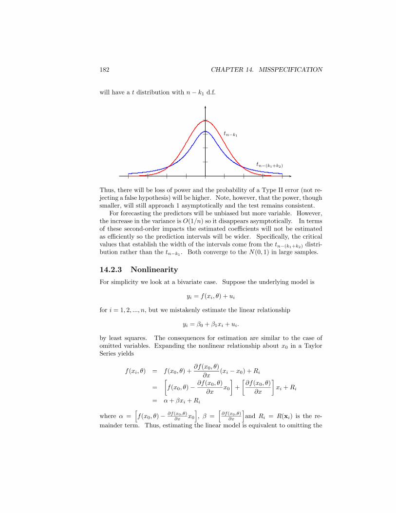
182 CHAPTER 14. MISSPECIFICATION
will have a t distribution with n− k1 d.f.
tn−(k1+k2)
tn−k1
Thus, there will be loss of power and the probability of a Type II error (not re-jecting a false hypothesis) will be higher. Note, however, that the power, thoughsmaller, will still approach 1 asymptotically and the test remains consistent.For forecasting the predictors will be unbiased but more variable. However,
the increase in the variance is O(1/n) so it disappears asymptotically. In termsof these second-order impacts the estimated coefficients will not be estimatedas efficiently so the prediction intervals will be wider. Specifically, the criticalvalues that establish the width of the intervals come from the tn−(k1+k2) distri-bution rather than the tn−k1 . Both converge to the N(0, 1) in large samples.
14.2.3 Nonlinearity
For simplicity we look at a bivariate case. Suppose the underlying model is
yi = f(xi, θ) + ui
for i = 1, 2, ..., n, but we mistakenly estimate the linear relationship
yi = β0 + β1xi + ui.
by least squares. The consequences for estimation are similar to the case ofomitted variables. Expanding the nonlinear relationship about x0 in a TaylorSeries yields
f(xi, θ) = f(x0, θ) +∂f(x0, θ)
∂x(xi − x0) +Ri
=
∙f(x0, θ)−
∂f(x0, θ)
∂xx0
¸+
∙∂f(x0, θ)
∂x
¸xi +Ri
= α+ βxi +Ri
where α =hf(x0, θ)− ∂f(x0,θ)
∂x x0
i, β =
h∂f(x0,θ)
∂x
iand Ri = R(xi) is the re-
mainder term. Thus, estimating the linear model is equivalent to omitting the

14.2. CONSEQUENCES OF MISSPECIFICATION 183
remainder term, which will be a function of xi. Note that the values of β and αdepend on the point of expansion so bα and bβ cannot be unbiased or consistentfor all values.For example, with a scatter of points generated by a concave nonlinear re-
lationship and then fitted by linear least squares we might have the followinggeometric relationship
f(xi)
yi
xi
α+ βxi
It is clear that: (a) the intercept is no longer correct, (b) the function yields theproper value at only two points, and (c) the slope of the estimated function iscorrect at only one point.The consequences for inference are similar to the case of omitted variables.
Even though a variable may be highly non-linearly related to yi, we may acceptbβj = 0 on a linear basis. Thus, we may commit Type II errors in choosing thecorrect variables.The consequences for prediction are evident. As a consequence of (b),
depending on the point of evaluation, we will either systematically over- orunder-estimate the regression function when used for conditional prediction.Depending on the nonlinearity, the farther we get from the estimated range, theworse the linear relationship will approximate f(xi).
14.2.4 Misspecified Disturbances
Suppose
yi = f(xi) + ui
is correct but we mistakenly estimate
yi = f(xi)u∗i .
(For example, suppose the true model is yi = αxβi + ui but we estimate yi =
αxβi u∗i or ln yi = lnα + β lnxi + lnu
∗i ). Solving for u∗i in the general case, we
obtain
u∗i =yi
f(xi)= 1 +
uif(xi)
.

184 CHAPTER 14. MISSPECIFICATION
So
E(u∗i ) = 1
var(u∗i2) =
σ2
f(xi)
Thus, the disturbances are heteroskedastic. If we transform into logs to obtainlinear in disturbance model, the transformed errors ln(u∗i ) = ln(1 +
uif(xi)
) will
still be heteroskedastic.Conversely, suppose the true model is
yi = f(xi)ui
with E[ui] = 1, but we mistakenly estimate
yi = f(xi) + u∗i
then
u∗i = f(xi)(1− ui)
and u∗i is conditional mean zero but heteroskedastic.The estimation, inferential, and prediction complications arising from het-
eroskedasticity are well-covered in Chapter 12. Likewise, the detection andcorrection of this problem is covered quite well there and will not be discussedbelow.
14.3 Detection of Misspecification
14.3.1 Testing for irrelevant variables
Suppose the model is
y = X1β1 +X2β2 + u
and we suspect that β2 = 0, i.e., X2 does not enter into the regression.We may test each coefficient of β2 directly using the test. Specifically, per-
form bβ = (X0X)−1X0y
the regression of y on X = (X1 : X2). Now,
bβjps2djj
∼ tn−k
under the null hypothesis that βj = 0. Thus, we can use the printed t-values totest whether the coefficients βj = 0.
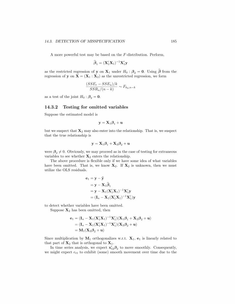
14.3. DETECTION OF MISSPECIFICATION 185
A more powerful test may be based on the F -distribution. Perform,bβ1 = (X01X1)
−1X01y
as the restricted regression of y on X1 under H0 : β2 = 0. Using bβ from theregression of y on X = (X1 : X2) as the unrestricted regression, we form
(SSEr − SSEu)/k
SSRu/(n− k)∼ Fk2,n−k
as a test of the joint H0 : β2 = 0.
14.3.2 Testing for omitted variables
Suppose the estimated model is
y = X1β1 + u
but we suspect thatX2 may also enter into the relationship. That is, we suspectthat the true relationship is
y = X1β1 +X2β2 + u
were β2 6= 0. Obviously, we may proceed as in the case of testing for extraneousvariables to see whether X2 enters the relationship.The above procedure is flexible only if we have some idea of what variables
have been omitted. That is, we know X2. If X2 is unknown, then we mustutilize the OLS residuals.
e1 = y− by= y−X1
bβ1= y−X1(X
01X1)
−1X01y
= (In −X1(X01X1)
−1X01)y
to detect whether variables have been omitted.Suppose X2 has been omitted, then
e1 = (In −X1(X01X1)
−1X01)(X1β1 +X2β2 + u)
= (In −X1(X01X1)
−1X01)(X2β2 + u)
=M1(X2β2 + u)
Since multiplication by M1 orthogonalizes w.r.t. X1, e1 is linearly related tothat part of X2 that is orthogonal to X1.In time series analysis, we expect x0t2β2 to move smoothly. Consequently,
we might expect et1 to exhibit (some) smooth movement over time due to the

186 CHAPTER 14. MISSPECIFICATION
relationship. That is
et1
t
0
Suppose xi1 and xi2 move together, i.e. are related in some fashion. The eiwill react non-linearly to changes in xi1 and hence x
0i1bβ = byi. Thus, a general
technique is to plot ei against byi = x0i1bβ. Under H0 : β2 = 0, we expect to findno relationship. If β2 6= 0, however et may have some relationship (nonlinear)to byt.
et
yt
0
This procedure may be formalized. Form the regression
et = γ1by2t + γ2by3t + vt
Under H0 : β2 = 0, et should be unrelated to xt1 and x0t1bβ = byt, i.e., γ1 = γ2 =
0. If this hypothesis is rejected by the regression results, we have evidence ofomitted variables.

14.3. DETECTION OF MISSPECIFICATION 187
14.3.3 Testing for Nonlinearity
Suppose the true regression is nonlinear:
yi = f(xi, θ) + ui
Expanding, as above about x0 in a Taylor Series, yields
yt = α+ βxi +Ri + ui
where Ri = R(xi) is the remainder term. In this case, since ei ≈ R(xi) + ui,then et will be a (nonlinear) function of xi. Thus, plots, of ei against xi willreveal a pattern:
ei
xi
0
Of course the pattern must be nonlinear in xi, since the OLS residuals ei areby definition linearly unrelated to the regressors.
A analogous formal test is to examine the regression
ei = γ0 + γ1x2i + γ2x
3i + vi
Under the null hypothesis of linearity, then ei is mean-zero and unrelated to xiwhereupon H0 : γ0 = γ1 = γ2 = 0. If nonlinearity is present we expect to findsignificant terms. Higher-order polynomials can be entertained but third-orderusually suffices.. In the multivariate case setting up all the various second-and third-order terms in the polynomial becomes more involved. Note that thelinear term is always omitted and the intercept is included in the null for powerpurposes.

188 CHAPTER 14. MISSPECIFICATION
14.4 Correcting Misspecification
14.4.1 Omitted or Extraneous Variables
If the two competing models are explicitly available then these two cases areeasily handled since one model nests the other. In the case of omitted vari-ables that should be included the solution is to include the variables if they areavailable. In the case of extraneous variables the solution is to eliminate theextraneous variables. The tests proposed in the previous section can be usedto guide these decisions.
If we have evidence of omitted variables but are uncertain of the nature ofthe omitted variables, then we need to undertake a model selection process todetermine the correct variables. This process is touched on below.
14.4.2 Nonlinearities
If we have evidence of nonlinearities in the relationship, then the solution in-volves entertaining a nonlinear regression. Usually, if we are proceeding froman initial linear model we have no idea of what the nature of the nonlinearityis but do know which variables to use. In the bivariate case, we can simplyintroduce higher-order polynomial terms, as in the testing approach, except wecontinue to include a linear term:
yi = β0 + β1xi ++β2x2i + β3x
3i + ui.
We can start with safe choice of the order of the polynomial and eliminateinsignificant higher-order terms. This process can be very involved when wehave a number of variables that are possibly nonlinear. This approach naturallyleads one to entertain nonparametric regression where we allow the regressionfunction to take on a very flexible form. These approaches have slower thannormal rates of convergence to the target function and are beyond the scope ofour analysis here.
Sometimes, we may have a specific nonlinear function in mind as the alter-native. For example, if the model was a Cobb-Douglas function and we decidedthat the log-linear form was inadequate due to heteroskedasticity, we might beinclined to estimate the nonlinear function directly with additive errors. Thisis the subject on nonlinear regression, which is given extended treatment in thenext chapter.

14.5. MODEL SELECTION APPROACHES 189
14.5 Model Selection Approaches
14.5.1 J-Statistic Approach
We begin with the simplified problem of choosing between two completely spec-ified models. Suppose the first model under consideration is
y = X1β1 + u1
but we suspect the alternative
y = X2β2 + u2
may be correct. How can we determine whether the first (or second) model ismisspecified? If the matrix X1 includes all the variables in X2 or visa versa,then the models are nested and we are dealing with possible extraneous variablesor possibly known omitted variables. These cases are treated above and thedecision can be made on the basis of an F -test.So we are left with the case where the two models are non-nested. Each
model includes explanatory variables that are not in the other. Davidson andMacKinnon (D-M) propose we consider a linear combination regression model
y = (1− λ)X1β1 + λX2β2 + u
= X1((1− λ)β1) +X2(λβ2) + u
= X1β∗1 +X2β
∗2 + u.
This formulation allows us to state the problem of which is the correct modelin parametric form. Specifically, we have H0 : Model 1 is correct or λ = 0 andH1 : Model 2 is correct or λ = 1. A complication arises, however, since neitherλ nor (1− λ) are identifiable but are subsumed into the scale of the parametervectors β∗1 and β
∗2.
Under the null hypothesis, however, the combined model simplifies to Model1, which suggests we just treat the combined regression in the usual way andjointly test for β∗2 = 0. The problem is that X1 and X2 may, and likely will,share variables (columns) so extreme collinearity will be a problem and theunrestricted regression is infeasible. However, any linear combination of thecolumns of X2 will also have a zero coefficient under the null. This suggeststhe following two-step approach: in the first regress y on X2 and calculate thefitted values, say by2 = X2(X
02X2)
−1X02y; in the second we regress using the
model
y = X1β∗1 + γby2 + u.
Under the null hypothesis, at least asymptotically, γ = 0, so we can just use theusual t-ratio, which is called the ”J-statistic” by D-M, to test whether γ = 0.If we fail to reject we conclude that Model 1 is correct.

190 CHAPTER 14. MISSPECIFICATION
If we reject, then we conclude that X2 adds important explanatory power toModel 1. We should now entertain the possibility that Model 2 is the correctmodel and run the test the other way, reversing the roles of Models 1 and 2.If we don’t reject the reversed hypotheses then we conclude that Model 2 iscorrect.
A very real possibility, and one that frequently occurs in practice, is that wereject going both ways, so neither Model 1 nor Model 2 is correct. This is aparticular problem in large samples since we know all models are misspecifiedat some level and this will be revealed asymptotically with consistent tests.Unfortunately, if we are still interested in choosing between the two models,this approach gives us no guidance. Thus the sequel of this section will dealwith how to choose between the models when they are both misspecified.
14.5.2 Residual Variance Approach
First, we will develop a metric that can be interpreted as a measure of misspec-ification. Now, for the first model we obtain
bβ1 = (X01X1)
−1X01y
e1 = y− by1= y−X1
bβ1= y−X1(X
01X1)
−1X01y
= (In −X1(X01X1)
−1X01)y
=M1y
and
s21 =e01e1n− k1
=y0M0
1M1y
n− k1=y0M1y
n− k1
Similarly, for the second model, we have
bβ2 = (X02X2)
−1X02y
and
s22 =y0M2y
n− k2
where M2 = (In −X2(X02X2)
−1X02)
Now, if the first model is correct
E[s21] = σ2

14.5. MODEL SELECTION APPROACHES 191
while
E[s22] = E
∙y0M2y
n− k2
¸= E
∙(X1β1 + u1)
0M2(X1β1 + u1)
n− k2
¸=
1
n− k2E [(X1β1 + u1)
0M2(X1β1 + u1)]
=1
n− k2E£β01X
01M2X1β + 2u
01M2X1β1 + u
01M2u1
¤=β01X
01M2X1β1n− k2
+ σ2 ≥ E[s2]
Thus, s2 is smallest, on average, for the correct specification. This suggests acriterion where we select the model with the smallest estimated variance. Thisis the residual-variance criterion. And the expression (β01X
01M2X1β1)/(n−k2)
can be taken as a measure of misspecification in terms of mean squared error.Provided that both models have the same dependent variable, which was
the case above, it is tempting to select between them on the basis of ”goodness-of-fit” or R2, which tells us the percentage of total variation in the dependentvariable that is explained by the model. The problem with this approach isthat R2 always rises as we add explanatory variables, so we would end up witha model using all possible explanatory variables whether or not they really enterthe relationship or not. Such a model would not work well out-of-sample if theextra variables move independently of the correctly included variables.A possible solution is to penalize the statistic for the number of included
regressors. Specifically, we propose the adjusted R2 statistic
R2= 1− n− 1
n− k(1−R2)
= 1− (e0e)/(n− k)Pni=1(yi − y)2/(n− 1)
= 1− s2Pni=1(yi − y)2/(n− 1)
Note that ranking models in terms of increasing R2is equivalent to ranking
them in terms of decreasing s2, since the other elements in the expression do
not change between models. One advantage of the R2approach is that it is
unit and scale-free.
14.5.3 A Model Selection Statistic
For the residual variance criterion, the rather obvious question is whether oneestimated variance is ”enough” larger than another to justify selection of one

192 CHAPTER 14. MISSPECIFICATION
model over another. We will formulate a test statistic as a guide in selectingbetween any two models. Specifically let
mi =n
n− k2(yi − x02ibβ2)2 − n
n− k1(yi − x01ibβ1)2
m =1
n
nXi=1
mi = s22 − s21
vm =1
n
nXi=1
(mi −m)2
and define
Dn =
√nm√vm
as our statistic of interest. Supposemp−→ 0, then under appropriate conditions
Dnd−→ N(0, 1) and tail occurrences (|Dn| > 1.96, say) would be rare events.Suppose that the true model is denoted by subscript 0, then m
p−→ 0 implies
s22 − s21p−→ 0 and hence
β01X01M0X1β1n−k0 − β02X
02M0X2β2n−k0
p−→ 0. If, from above,
we takeβ0lX
0lM0Xlβln−k0 as an index of misspecification of the model l relative to
the true model 0, then we see that mp−→ 0 indicates that the two models are
equally misspecified. This leaves us with three possibilities
(1) Model 1 is ”equivalent” to Model 2: Dnd−→ N(0, 1)
(2) Model 1 is ”better” than Model 2: Dna.s.−→ +∞
(3) Model 2 is ”better” than Model 1: Dna.s.−→ −∞.
Large positive values favor Model 1. Large negative value favor Model 2. Theintermediate values (e.g. |Dn| > 1.96 for 95 percent significance) comprise aninconclusive region.
14.5.4 Stepwise Regression
In the above model selection approaches, we have reduced the number of com-peting models to a small number before undertaking statistical inference. Suchreductions are usually guided by competing economic theories and experiencefrom previous empirical exercises. Such reductions are really at the heart ofeconometrics which is seen as the intersection of data, economic theory, andstatistical analysis. The model we end up with really depends on all threecontributors to winnow the competing models down to a select few. Such anapproach is at the heart of structural and even informed reduced form modeling.It is of interest to think about the model selection process from a more data-
driven standpoint. This might be the case if economic theory does not give

14.5. MODEL SELECTION APPROACHES 193
firm guidance as to which explanatory variables enter the relationship for whichdependent variable. Such a situation might be characterized by the true modelhaving the form
y = X1β1 + u1
where the variables comprising X1 are not known but are a subset of the avail-able economic variablesX. Somehow, we would like to use the data to determinethe variables entering the relationship. Unfortunately, some problems arise inany purely data-driven approach as we will see below.At this point, it seems appropriate to compare the consequences of incor-
rectly omitting a variable against incorrectly including an extraneous variable.They are really two sides of the same coin but the consequences are very dif-ferent. Omitting the variable incorrectly leads to bias and inconsistency andincorrect size due to increased probability of a Type I error. Including anextraneous variable increases the probability of a Type II error and hence de-creased power but the test will still be consistent. Thus we are faced with theoft encountered trade-off between size and power in deciding how to conductinference.In the usual inferential exercise we carefully calibrate the test so that the
size takes on a prespecified value, such as .05 and take the power that results.Implicitly, this approach places greater value on getting the size correct at theexpense of power and the consequences of omitted variables should be viewedas more serious than those of including extraneous variables. This suggests the”kitchen-sink” approach when deciding which variables to include in the modelunder construction. When in doubt, leave it in, would seem to be good advicebased on this reasoning.An approach suggested by this reasoning is the backward elimination step-
wise regression approach. In this approach, we start with a regression includingall candidate regressors and eliminate them one-by-one on the basis of statisti-cal insignificance. The resulting regression model will have all the regressorsstatistically significant, at some level, by the measure used. An example ofa decision criterion at each step would be to eliminate the variable with thehighest t-ratio until the remaining t-ratios are no smaller than one. At this
point the elimination of any of the remaining variables would reduce the R2and
not be preferred.There are a couple of problems with this approach. The first is the fact that
we do not necessarily end up with the best set of regressors that are significant.Some variables that were eliminated in early rounds may end up being veryimportant once others have been eliminated. A modification is to entertain allpossible competing models that have a given number of explanatory variables,but this becomes very complicated when the number of variables in X is large.A second problem is that the regression model that results from this process
would not have standard statistical properties. This is easily seen. The usualratios on the estimated coefficients could not have a t distribution because small

194 CHAPTER 14. MISSPECIFICATION
values of the ratio have been eliminated in the selection process. For exampleall the ratios would be larger in absolute value than, say 1. Nor could they evenbe normal in large samples. This is an example of what is called pre-test bias.If parts of a model have been selected on the basis of a previous testing step,the properties of tests in the current step will not have the usual properties.The serious problems with the stepwise regression approach indicated by the
non-standard distribution can be seen as resulting from data-mining. Supposewe start out with a variable yi, which we label as the dependent variable, and alarge set of other variables, which we label as candidate regressors. In additionsuppose that the candidate regressors have been randomly generated and bearno true relationship to the dependent variable. If the sample size is not largeand the number of candidate regressors is large, then just by chance a subset ofthe regressors will be correlated with the dependent variable.Specifically, a subset will have a large t-ratio just by chance. This is also
easy to see. The true regression coefficients are all zero so the t-ratios will havea t-distribution and a certain fraction, say 0.16 for 30 degrees of freedom, willhave t-ratios larger than 1. But this is purely a result of spurious correlation.Thus we see that the stepwise regression approach is fraught with difficulties. Itis really a pure data-mining approach and cannot be expected to yield importanteconomic insights. Instead we should let our choice of variables and modelsbe guided to the extent possible by economic theory and previous econometricresults.