MULTI-VECTOR EMBEDDING ON NETWORKS WITH TAXONOMIES

Under review as a conference paper at ICLR 2022

MULTI-VECTOR EMBEDDING ON NETWORKS WITHTAXONOMIES

Anonymous authorsPaper under double-blind review

ABSTRACT

Networks serve as efficient tools to describe close relationships among nodes.Taxonomies consist of labels organized into hierarchical structures and are oftenemployed to describe rich attributes of the network nodes. Existing methods thatco-embed nodes and labels in a low-dimensional space all encounter an obstaclecalled under-fitting, which occurs when the vector of a node is obliged to fit allits labels and neighbor nodes. In this paper, we propose HIerarchical Multi-vectorEmbedding (HIME), which allows multiple vectors of a node to fit different setsof its labels in a Poincare ball, where the label hierarchy is well preserved. Ex-periments show that HIME has comprehensive advantages over existing networkembedding methods in preserving both node-node and node-label relationships.

1 INTRODUCTION

A network is usually applied to depict the proximities among nodes, with extra node properties de-scribed by labels organized as a taxonomy. For instance, in a co-authorship network with a researchtaxonomy, a network edge between two researchers reveals their close academic relationship, whilethe hierarchical labels ’artificial intelligence’, ’natural language processing’ and ’sentiment analysis’formed into a label-path in the taxonomy reveal a researcher’s areas of interest. Generally, a nodecan have multiple label-paths in the taxonomy telling different properties, as shown in figure 1 (a).

Heterogeneous network embedding serves as an option for co-embedding nodes and labels. It learnsa low-dimensional vector for each entity, so that the distances among the embedding vectors indicatethe topographic distances among entities in the network with the taxonomy. However, the singleembedding vector of a node can be overloaded to preserve both the node-node and the node-labelrelationships, which causes the under-fitting problem Yang et al. (2020). As illustrated in figure 1(b), single-vector embedding methods will possibly embed a node in the middle of all its labels inorder to minimize the overall node-label distances, resulting in the node not being close to any of itslabels. The under-fitting problem seriously worsens the performance on the distance-related tasks,such as label retrieval for a certain node according to the node-label distances.

To solve the under-fitting problems, one way is to reform the embedding position of the labels soas to minimize the chances of under-fitting, which can be achieved by using hyperbolic spaces. Ahyperbolic space is a non-Euclidean space, and it grows exponentially with the increase of the spaceradius. It can be viewed as a continuous version of trees, which naturally caters to the hierarchicallabel structure Nickel & Kiela (2017). Labels in a label-path are embedded in the same directionin the hyperbolic space, so that a node vector is less likely to under-fit the labels belonging to asingle label-path. But simply using hyperbolic embedding technique does not necessarily tackle theunder-fitting problem, since a node can have multiple label-paths in different directions. However,by allocating multiple vectors to a node, with each fitting a small set of labels as shown in figure 1(c), the under-fitting problem can be well resolved.

Therefore, we propose HIerarchical Multi-vector Embedding (HIME), which co-embeds networknodes and taxonomy labels in a hyperbolic space. HIME gives each label a single embedding vec-tor to preserve the hierarchical structure, while a node has multiple vectors, with one specializedin maintaining the node-node proximity, and the others overcoming the under-fitting problem inpreserving the node-label relationships.

1


A

B

E

C

G

Single-Vector Embedding Multi-Vector EmbeddingNetwork and Taxonomy

A

B C

D E F G H

(a) (b) (c)

AB

E

C

G

Figure 1: The difference between single-vector embedding and multi-vector embedding. Given anetwork node with five circled labels in a taxonomy (a), single-vector embedding learns a vectorin the middle of all the five labels, which leads to under-fitting (b). However, by learning multiplevectors for a node, the under-fitting problem can be overcome in a Poincare disk (c).

Our work makes the following contributions: (1) We solve the under-fitting problem by allowingmultiple embedding vectors of a node to fit different sets of labels. (2) A Least Recently Used(LRU) based algorithm balances the loads on the multiple vectors of a node. (3) Hyperbolic spacesare applied to co-embed network nodes and hierarchical labels more effectively. (4) Experimentsshow that HIME has better capability of preserving both node-node and node-label relationshipscompared with existing network embedding methods.

2 RELATED WORK

In this section, we first introduce some classic approaches of network embedding, followed by thetaxonomy-related embedding methods most relevant to our background. Hyperbolic embeddingmethods will then be presented. Finally we will introduce the concept of multi-aspect embedding.

Network Embedding. Approaches of network embedding can be mainly categorized into matrixfactorization, Skip-Gram with walk patterns Mikolov et al. (2013) and neural networks from theperspective of methodology. Algorithms based on matrix factorization Belkin & Niyogi (2003); Caoet al. (2015); Ou et al. (2016) obtain embedding vectors by factorizing either Laplacian eigenmaps orthe node proximity matrix. Methods using Skip-Gram model with walk patterns are prevailed in bothplain network embedding Perozzi et al. (2014); Grover & Leskovec (2016); Tang et al. (2015b), andheterogeneous network embedding Dong et al. (2017); Tang et al. (2015a); Hussein et al. (2018).The neural network based methods Kipf & Welling (2016); Hamilton et al. (2017); Wang et al.(2018; 2016); Cao et al. (2016); Fu et al. (2017) generate the embedding vectors by ways such asgraph convolution and adversarial training Goodfellow et al. (2014). Though not customized fornetworks with taxonomies, these classic methods laid the foundation for later embedding methodsvarying for different tasks or data.

Taxonomy-Related Embedding. Several embedding methods on networks with taxonomies havebeen proposed in recent years. Onto2Vec Smaili et al. (2018) first learns the embedding vectorsof the biomedical taxonomy, and then generates the vectors for biological entities based on thelearned taxonomy vectors. The drawback of Onto2Vec is that it ignores the label co-occurrenceswhen learning the vectors for labels. Tag2Vec Wang et al. (2019) applies meta-path patterns andco-embeds nodes and hierarchical labels, while it still suffers from the under-fitting problem when anode has multiple label-paths. Given a label in the taxonomy, TaxoGAN Yang et al. (2020) spares anindividual embedding space for it, where its nodes and its child labels are embedded by adversarialtraining. Although TaxoGAN well preserves the node-label proximity in small sub-graphs, it failsto maintain the node-label relationships globally. The key issue of embedding lies in using globallyfunctional vectors to overcome the under-fitting problem, which has not been well addressed byexisting taxonomy-related methods.

2


Hyperbolic Embedding. Previous researches have shown that preserving hierarchical structuresin Euclidean space requires large embedding dimension Nickel et al. (2014), while it can be eas-ily achieved by using low-dimensional hyperbolic spaces Gromov (1987); Boguna et al. (2010).HGCN Chami et al. (2019) embeds nodes by using graph convolution operation defined in hyper-bolic spaces. Poincare Nickel & Kiela (2017) embeds words into a Poincare ball so as to maintain thehypernym relationships, while HMLC Chen et al. (2020) performs hierarchical multi-label text clas-sification by co-embedding words and labels into a hyperbolic space. The success of single-vectorhyperbolic embedding on words mainly attributes to the fact that most words are univocal in thehierarchy. However, these methods are not capable of representing nodes with multiple label-paths.

Multi-Aspect Embedding. Contrast to existing single-vector embedding methods, several recentworks have revealed the necessity of learning multiple vectors for each node in different aspects.PolyDW Liu et al. (2019) represents each facet of an item using an embedding vector; SplitterEpasto & Perozzi (2019) allows multiple node embedding vectors to encode different communities;Asp2Vec Park et al. (2020) employs random walks to dynamically assign aspects to each nodeaccording to its local context; JOIE Hao et al. (2019) presents a two-view embedding model fora knowledge graph. Though innovative, most multi-aspect methods preserve relationships amongnodes in different aspects, while neglecting either node-aspect proximity or hierarchical structures.Differently, HIME preserve both node-node and node-label relationships under the label hierarchy.

3 PRELIMINARIES

In this part, we will first formally define our problem, and introduce the notations used throughoutthe paper. Then we will briefly describe the Poincare ball where nodes and labels are embedded.

3.1 PROBLEM STATEMENT

HIME takes the following data as inputs:

• a network N = {V,E}, where V = {vi}, i = 1, 2, .., n is the set of nodes, and E ={eij}, i, j = 1, 2, .., n, i 6= j is the set of edges;

• a label taxonomy T = {L, S}, where L = {li}, i = 1, 2, ...,m is the set of labels, andS = {sij}, i, j = 1, 2, ...,m, i 6= j is the set of parent-child edges;

• a label assignment A = {Ai}, i = 1, 2, ..., n, where Ai is the set of labels that node vi has.Once a label appears in Ai, all its ancestors in the taxonomy will also appear in Ai.

Given the inputs, HIME learns a single vector for each label and multiple vectors for each node.Specifically, every node has a single ’root vector’ to preserve node proximity, and several ’branchvectors’ to fit its labels. Formally, given dimension d and branch vector number k, HIME produces:

• The root vectors Rn×d of the nodes, with Ri referring to the root vector of vi;• The branch vectors Bn×k×d of the nodes, with Bij , i = 1, 2, .., n, j = 1, 2, ..., k referring

to the j-th branch vector of vi;• The label vectors Qm×d, with Qi referring to the representation vector of li.

In this way, R preserves the node proximity, Q preserves the hierarchical taxonomy, while B and Qtogether preserve the node-label relationships. All vectors function in a Poincare Ball as follows.

3.2 THE POINCARE BALL MODEL

Let ‖·‖ denotes the Euclidean norm. A Poincare ball with dimension d and radius 1 can be defined as:Dd,1 := {x ∈ Rd : ‖x‖2 < 1}, gx = λ2xId, where gx is the Riemannian metric tensor, λx = 2

1−‖x‖2

and Id is the identity matrix. The distance between two points x, y ∈ Dd,1 can be computed as:

dist(x, y) = arcosh

(1 + 2

‖x− y‖2

(1− ‖x‖2)(1− ‖y‖2)

). (1)

Though having limited radius, the Poincare ball has infinite space volume. A hierarchical structurecan be embedded in the ball by placing the root near the center while leaves near the open surface.

3


4 METHOD

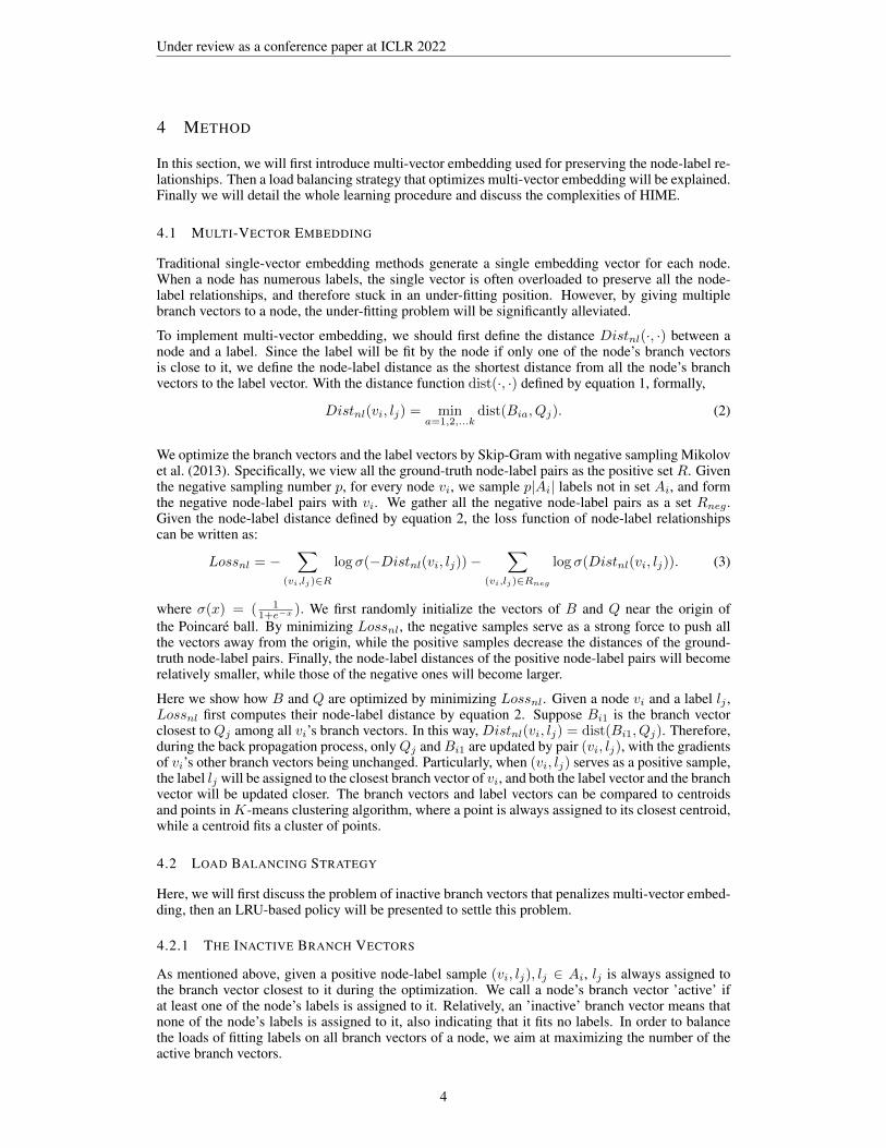
In this section, we will first introduce multi-vector embedding used for preserving the node-label re-lationships. Then a load balancing strategy that optimizes multi-vector embedding will be explained.Finally we will detail the whole learning procedure and discuss the complexities of HIME.

4.1 MULTI-VECTOR EMBEDDING

Traditional single-vector embedding methods generate a single embedding vector for each node.When a node has numerous labels, the single vector is often overloaded to preserve all the node-label relationships, and therefore stuck in an under-fitting position. However, by giving multiplebranch vectors to a node, the under-fitting problem will be significantly alleviated.

To implement multi-vector embedding, we should first define the distance Distnl(·, ·) between anode and a label. Since the label will be fit by the node if only one of the node’s branch vectorsis close to it, we define the node-label distance as the shortest distance from all the node’s branchvectors to the label vector. With the distance function dist(·, ·) defined by equation 1, formally,

Distnl(vi, lj) = mina=1,2,...k

dist(Bia, Qj). (2)

We optimize the branch vectors and the label vectors by Skip-Gram with negative sampling Mikolovet al. (2013). Specifically, we view all the ground-truth node-label pairs as the positive set R. Giventhe negative sampling number p, for every node vi, we sample p|Ai| labels not in set Ai, and formthe negative node-label pairs with vi. We gather all the negative node-label pairs as a set Rneg .Given the node-label distance defined by equation 2, the loss function of node-label relationshipscan be written as:

Lossnl = −∑

(vi,lj)∈R

log σ(−Distnl(vi, lj))−∑

(vi,lj)∈Rneg

log σ(Distnl(vi, lj)). (3)

where σ(x) = ( 11+e−x ). We first randomly initialize the vectors of B and Q near the origin of

the Poincare ball. By minimizing Lossnl, the negative samples serve as a strong force to push allthe vectors away from the origin, while the positive samples decrease the distances of the ground-truth node-label pairs. Finally, the node-label distances of the positive node-label pairs will becomerelatively smaller, while those of the negative ones will become larger.

Here we show how B and Q are optimized by minimizing Lossnl. Given a node vi and a label lj ,Lossnl first computes their node-label distance by equation 2. Suppose Bi1 is the branch vectorclosest to Qj among all vi’s branch vectors. In this way, Distnl(vi, lj) = dist(Bi1, Qj). Therefore,during the back propagation process, onlyQj andBi1 are updated by pair (vi, lj), with the gradientsof vi’s other branch vectors being unchanged. Particularly, when (vi, lj) serves as a positive sample,the label lj will be assigned to the closest branch vector of vi, and both the label vector and the branchvector will be updated closer. The branch vectors and label vectors can be compared to centroidsand points in K-means clustering algorithm, where a point is always assigned to its closest centroid,while a centroid fits a cluster of points.

4.2 LOAD BALANCING STRATEGY

Here, we will first discuss the problem of inactive branch vectors that penalizes multi-vector embed-ding, then an LRU-based policy will be presented to settle this problem.

4.2.1 THE INACTIVE BRANCH VECTORS

As mentioned above, given a positive node-label sample (vi, lj), lj ∈ Ai, lj is always assigned tothe branch vector closest to it during the optimization. We call a node’s branch vector ’active’ ifat least one of the node’s labels is assigned to it. Relatively, an ’inactive’ branch vector means thatnone of the node’s labels is assigned to it, also indicating that it fits no labels. In order to balancethe loads of fitting labels on all branch vectors of a node, we aim at maximizing the number of theactive branch vectors.

4


1

2

3

1 1

1 1 1

3

3

3 3

32 2

22

2

(a)

(f)

(b)

(e) (d)

(c)

Figure 2: An illustration of the LRU replacement policy. Three red branch vectors are allocated tofit the blue labels, with one continuously being lazy (a). After two LRU periods (b)-(c) and (d)-(e), finally each branch vector fits a small set of labels (f). In real cases, the label vectors are alsoupdated, and the geodesic line between any two points in a 2D Poincare disk is actually a curve.

For a node having a small number q of labels where q < k, unavoidably, at least k − q inactivebranch vectors exist at any time. However, there is no guarantee that all the k branch vectors will beactive if q > k. Consider situation (a) shown in figure 2. A node is given k = 3 red branch vectorsto fit its q = 7 blue labels, with the third branch vector being inactive since it is not the closestto any labels. Given the node-label loss function in equation 3 and the node-label distance definedby equation 2, in the following iterations, the presently active branch vectors will be continuallyupdated by the positive node-label pairs of the node, with the inactive branch vector never beingoptimized positively. Therefore, the second branch vector is continually pulled by five labels andstuck in an under-fitting position, with contrast to the third branch vector always being lazy.

It should be pointed out that a node is allowed to have less than k active branch vectors, which issimilar toK-means clustering algorithm having less thanK active centroids. But in order to preventthe unbalanced loads shown in figure 2 (a), we aim at making the most of the k branch vectors. Wepresent a solution to the unbalanced loads based on the LRU algorithm.

4.2.2 THE VECTOR REPLACEMENT POLICY

The least recently used (LRU) algorithm originally describes a cache replacement policy that swapsout the least recently used cache pages to make room for frequently used pages. Here, we apply theLRU algorithm to balance the loads among different branch vectors. The main idea is to move aninactive branch vector to a place near the most active branch vector so as to share the burden of it.

Figure 2 illustrates the optimization process using the LRU policy. In (b), a vector replacement isperformed, and branch vector 3 is replaced by a new vector close to branch vector 2, with theirmargin being 10−3 ∗ ε, where ε is a random normal distribution vector. Extreme cases exist thatthe new vector attracts all the labels of the original vector, as shown in (c), causing the previouslyactive branch vector 2 becomes inactive. However, iterations of the LRU policy will finally achievea correct vector replacement. As illustrated in (d), after an LRU period, the inactive branch vector 2is relocated so that branch vectors 2 and 3 each attracts a set of labels, which is shown in (e). Finallyeach of the three branch vectors is optimized to fit a small group of labels, as shown in (f).

In the implementation, we maintain a hit matrix Hn×k to support the LRU algorithm. Specifically,Hij record the hit number ofBij . A hit ofBij means thatBij fits a label of node vi. H can be simplymaintained by sending a Boolean variable to the function 2 that calculates node-label distances. TheBoolean variable indicates whether the node-label pairs are positive samples. Specifically, if a node-

5


Algorithm 1 The whole learning process.Input: network N , label taxonomy T , label assignment A, dimension d, the branch vector number

k, negative sampling number p, epoch number g, LRU period tOutput: root vectors R, branch vectors B, label vectors Q1: initialize H = 0; randomly initialize B, R and Q near the origin of the Poincare Ball2: for epoch in {1, 2, ..., g} do3: negatively sample label-label, node-label and node-node pairs4: compute Lossll and update Q by batches5: compute Lossnl and update Q and B by batches meanwhile maintaining H6: compute Lossnn and update R by batches7: if epoch mod t == 0 then8: update B by the LRU algorithm9: H = 0

10: end if11: end for12: output R, B, Q and H

label pair is a positive sample, the function will remember the index a of the branch vector that fitsthe label, and then plus Hia by 1 to record a hit. After a period of optimization, for every node withinactive branch vectors, we replace one of its inactive vectors with a new vector initialized close tothe active branch vector with the highest hit value. We then clear H to 0 for the next LRU period.

4.3 THE WHOLE LEARNING PROCESS OF HIME

There are three kinds of relationships that need to be preserved: the node-node relationships pre-sented by the network N , the label-label relationships given by the taxonomy T , and the node-labelrelationships revealed by the label assignment A. We have mainly discussed how to preserve node-label relationships by multi-vector embedding. Here we briefly present the loss functions of thenode-node and label-label relationships.

Node-Node Relationships. Node-node relationships are reflected by the edges of the network N .Each node vi has a single root vector Ri, and we use the root vectors to preserve the node-noderelationships. Given the edge set E of the network N , let E denote the set of edges not being in E.For every edge eij in E, we negatively sample p edges from E either connecting node vi or nodevj . We combine these edges into a set of negative samples Eneg . With equation 1 calculating thedistance between two vectors, we aim at minimizing the following loss function:

Lossnn = −∑

eij∈Elog σ(−dist(Ri, Rj))−

∑eij∈Eneg

log σ(dist(Ri, Rj)), (4)

Label-Label Relationships. The label-label relationships are given by the label hierarchy T ={L, S}, where S = {sij}, i, j = 1, 2, ...,m contains the parent-child relationships between labelpairs. Here, we view edges in S as un-directed. Similarly, we take the edges in S as positivesamples, and for every edge sij in S, we negatively sample p edges from S connecting either lior lj , where S is the complementary set of S. We gather these negative samples as set Sneg . Theobjective function of label-label relationships is:

Lossll = −∑sij∈S

log σ(−dist(Qi, Qj))−∑

sij∈Sneg

log σ(dist(Qi, Qj)). (5)

Given the three Loss functions 3, 4 and 5, the learning process aims at minimizing the followingloss function:

Losstotal = Lossnn + Lossll + Lossnl.

During the back propagation, we use Riemannian Stochastic Gradient Descent (RSGD) Bonnabel(2013) to update R, B and Q in the Poincare ball.

Algorithm 1 shows the whole learning process of HIME. The space complexity of HIME is O((1 +k)|V |d+|L|d), which is the space occupied byR,B andQ. For simplicity, we use |A| to refer to the

6


total number of ground-truth node-label pairs. Given the predetermined negative sampling numberp, during each epoch, (1 + p)|S| label-label pairs, (1 + p)|A| node-label pairs and (1 + p)|E|node-node pairs are passed to the model. The extra cost of our method lies in the minimizationcomputation defined by equation 2, which is O(k). Therefore the total time complexity of learningfor g epochs is O(gp|S| + gkp|A| + gp|E|), which grows linearly with the increase of the branchvector number k.

5 EXPERIMENTS

We conduct the experiments on datasets from different domains to evaluate HIME’s performance inpreserving node-label and node-node relationships compared with existing methods.

DBLP. Yang et al. combines a DBLP co-authorship network with ACM research taxonomy. Thenodes are authors, and the labels are hierarchical key words. A label will be assigned to an authorif the paper of the author contains that key word. Based on their dataset, we extract a dense sub-network containing 12379 nodes and 268 labels organized into a 4-level hierarchy. Our DBLPdataset has 12164 un-directed node-node links and 50402 node-label links, therefore a node has1.97 neighbor nodes and 4.07 labels on average.

STRING-GO. We use the protein-protein interaction network of humans from STRING databaseSzklarczyk et al. (2021) ,with the Cellular Components domain of Gene Ontology (GO) Ashburneret al. (2000); GO2 (2021) being the taxonomy. The GO annotation of human proteins is given byGOA database Camon et al. (2004); Huntley et al. (2015). The STRING-GO dataset consists of13840 nodes and 4184 labels organized into a 4-level DAG, and has 348658 un-directed node-nodelinks and 205629 node-label links. On average, a node has 50.38 neighbor nodes and 14.86 labels.

Methods for Comparison. We include 7 existing network embedding methods either classic orstate-of-the-art for comparison. Node2Vec Grover & Leskovec (2016), LINE Tang et al. (2015b)and GraphGAN Wang et al. (2018) deal with plain networks, and we run these methods by viewinglabels as plain nodes and label-related edges as plain edges. GraphSAGE Hamilton et al. (2017),PTE Tang et al. (2015a) and TaxoGAN Yang et al. (2020) are embedding methods on heterogenousor attributed networks, among which TaxoGAN is the state-of-the-art method on networks withtaxonomies. We also include Poincare Nickel & Kiela (2017), which embeds nodes and labels in thePoincare Ball to better preserve the hierarchical structures. In the experiments, we set the embeddingdimension of all methods to 256. We test HIME with k being 2, 4 and 8, and therefore the dimensionof branch vectors are 128, 64, 32 respectively so as to ensure that HIME has the total dimension of256. All methods are trained for 50 epochs.

5.1 NODE-LABEL RELATIONSHIPS

We design three tasks to evaluate the performance of all methods in preserving node-label relation-ships, namely label retrieval, label-path retrieval and node retrieval. For better describing the tasks,we first define the proximity score of two objects as the inner product of their representation vec-tors for methods in Euclidean spaces. For HIME and Poincare, the score is the negative hyperbolicdistance between the two vectors.

Label Retrieval. In the Label-retrieval task, given a node, the method should recall all the ground-truth labels of the node by ranking the scores of all labels with regard to that node. We use theMean Rank MR of the ground-truth labels to evaluate the label-retrieval performance on a node.We average the MR over all nodes to obtain MR.

Label-Path Retrieval. The label-path retrieval task evaluates a method’s capability of retrieving acorrect label-path for a node. Given the node, the method first predicts the label with the highestscore at the top level of the taxonomy. If the predicted label falls into one of the node’s label-path, then the prediction will move to the sub-tree rooted at the predicted label. The prediction willcontinue until either a false prediction occurs or the whole label-path is predicted correctly. Theaccuracy Acc is computed as the ratio of the number of accurately predicted labels to the label-pathlength. We use Acc averaged over all nodes to evaluate the label-path retrieval performance.

Node Retrieval. Given a label, the node-retrieval task aims at ranking the nodes of that label aheadof those not belonging to that label. The method ranks the scores of all nodes with regard to the

7

https://dblp.uni-trier.de/xml

https://dl.acm.org


Table 1: The experiments on the two datasets with the embedding dimensions of all methods being256. The dimensions of vectors of HIME 2, HIME 4, HIME 8 are 128, 64 and 32 respectively,satisfying the constraint that all methods have 256 dimensions.

DBLP node-label node-node label-label

MR Acc AUPRC AUPRC AUROC MR

TaxoGAN 124.61 54.60 4.53 99.53 99.92 136.81Node2Vec 111.20 33.59 11.23 94.58 97.59 68.67

LINE 85.57 29.83 27.85 82.79 92.74 80.40GraphSAGE 58.27 66.46 27.56 65.39 87.62 81.51GraphGAN 90.74 25.53 35.00 99.88 99.98 76.95

PTE 172.48 10.80 5.04 81.84 92.85 144.71Poincare 23.72 52.39 45.69 96.12 98.92 81.20HIME 2 7.72 87.39 91.26 98.47 99.13 50.81HIME 4 7.36 87.44 96.51 98.38 99.10 49.75HIME 8 6.69 68.95 76.61 97.25 98.42 68.44

STRING-GO node-label node-node label-label

MR Acc AUPRC AUPRC AUROC MR

TaxoGAN 2356.12 73.71 4.69 91.09 96.77 2053.35Node2Vec 617.73 12.80 19.10 69.49 87.36 611.01


PTE 2891.33 10.98 5.07 79.68 92.35 1644.75Poincare 110.39 18.12 22.10 85.90 93.10 710.47HIME 2 91.33 26.00 53.64 86.59 94.84 596.30HIME 4 86.44 17.93 70.16 86.64 94.91 562.49HIME 8 90.30 19.13 78.85 86.70 94.98 584.19

label, and we use the Area Under the Precision-Recall Curve AUPRC to evaluate the ranking. Wethen average the AUPRC over all labels to obtain AUPRC evaluating the overall performance.

The three ’node-label’ columns of table 1 correspond to the three tasks. In the label retrieval task,HIME and Poincare are the best two methods on both datasets, mainly because the Poincare Ballhas more embedding capacity compared to its Euclidean counterparts with the same dimension.Moreover, HIME performs slightly better than Poincare, in that HIME minimizes the distancesbetween a node and its labels by using multiple branch vectors, causing the ground-truth labelsranked further ahead.

In the label-path retrieval task, HIME and TaxoGAN are the two methods having the overall bestperformances on both DBLP and STRING-GO, mainly because they both allow multiple vectors ofa node in essence. On DBLP, HIME obtains higher Acc than TaxoGAN, While on STRING-GO,TaxoGAN outperforms all other algorithms with a considerable margin. This is because TaxoGAN isspecialized in retrieving a node’s ground-truth label from the label’s siblings by embedding them intoa small sub-graph. Compared to DBLP which has only 268 labels, STRING-GO has 4184 labels,which makes the effect of decomposing the taxonomy into different sub-graphs more remarkable.However, the drawback of decomposition is also obvious since the embedding vectors of the nodesonly function locally in different sub-graphs, and this side-effect will be revealed by the task of noderetrieval as follows.

By allowing multiple globally functional vectors of a node, HIME significantly outperforms all othermethods on the task of node retrieval. HIME 4 and HIME 8 are the best on DBLP and STRING-GOrespectively. By contrast, TaxoGAN performs poorly on the node-retrieval task. This is because inTaxoGAN, a local embedding vector of a node is not able to reflect the node’s relationship witha label outside of the sub-graph. Therefore, the scores between most node-label pairs are almostrandom, which accounts for the poor ranking performance of TaxoGAN.

8


natural language processing

sentiment analysis

information retrieval

artificial intelligence

retrieval tasks and goals

HIME_2

natural language processing sentiment analysis

information retrievalartificial intelligence


HIME_4


sentiment analysis

information retrievalartificial intelligence


HIME_8

Figure 3: The research areas of an author in a 2D Poincare disk. The blue points are the hierarchicallabels, with the red points being the author’s active branch vectors. ’Information retrieval’ and’retrieval tasks and goals’ are embedded apart in HIME 8.

5.2 NODE-NODE RELATIONSHIPS

We apply the task of node-pair retrieval to evaluate the performance in preserving node-node rela-tionships. Specifically, we randomly sample positive and negative node-node pairs, with their ratiobeing 1:4. The methods calculate the score of every node-node pair, and generate a ranking for allnode-node pairs. We use AUPRC and AUROC to evaluate the node-node pair retrieval performance.

The columns of ’node-node’ in table 1 display the results of node-pair retrieval. GraphGAN hasthe highest AUPRC and AUROC values compared to other methods, followed by TaxoGAN, HIMEand Poincare. The power of adversarial training can be inferred from the good performance ofTaxoGAN and GraphGAN. Though not the best on the node-node pair retrieval task, HIME performsbetter than other Euclidean and hyperbolic methods. The success of HIME in preserving node-noderelationships can be partly attributed to the branch vectors, which liberate the root vectors from theburden of fitting labels.

5.3 LABEL-LABEL RELATIONSHIPS

We use the retrieval of parent-child edges to evaluate the preservation of label taxonomy. Given alabel, the methods rank the scores of all other labels with respect to the label. We use the MeanRank MR of the its immediate child labels to evaluate the preservation of hierarchy. We averagethe MR over all labels to obtain MR.

The ’label-label’ column in table 1 shows the results. HIME, Poincare and Node2Vec are the threebest methods, with HIME 4 being the best on both DBLP an STRING-GO. It can be seen fromfigure 3 and table 1 that the hierarchical label structure of HIME 8 is not well preserved comparedto that of HIME 2 and HIME 4. This is because the label vectors are mainly optimized by Lossnl.When k increases, the branch vectors of nodes are given more degrees of freedom than the labelvectors. The decrease of Lossnl is mainly contributed to the branch vectors instead of the labelvectors, causing the label vectors being optimized insufficiently. Therefore, we recommend settingk less than 5 so as to gain a significant increase in performance compared to single-vector embeddingmethods, meanwhile keeping a low time complexity.

6 CONCLUSIONS

We propose a method called HIME, which endows a node with multiple vectors to alleviate theeffect of under-fitting in the hyperbolic embedding space. Our multi-vector embedding can be easilyextended to Euclidean spaces by simply changing the distance function, and can also be applied inplain networks where a node belongs to multiple communities. We point out that though multiplevectors can help preserving the node’s relationships with labels, they may also distort the labelhierarchy by over-fitting. Therefore, we suggest setting a small multi-vector number so as to achievea notable improvement in performance with a small time cost. But how to strike an embeddingbalance between the node-label relationships and the label hierarchy awaits future researches.

9


REFERENCES

The gene ontology resource: enriching a gold mine. Nucleic Acids Research, 49(D1):D325–D334,2021.

Michael Ashburner, Catherine A Ball, Judith A Blake, David Botstein, Heather Butler, J MichaelCherry, Allan P Davis, Kara Dolinski, Selina S Dwight, Janan T Eppig, et al. Gene ontology: toolfor the unification of biology. Nature genetics, 25(1):25–29, 2000.

Mikhail Belkin and Partha Niyogi. Laplacian eigenmaps for dimensionality reduction and datarepresentation. Neural computation, 15(6):1373–1396, 2003.

Marian Boguna, Fragkiskos Papadopoulos, and Dmitri Krioukov. Sustaining the internet with hy-perbolic mapping. Nature communications, 1(1):1–8, 2010.

Silvere Bonnabel. Stochastic gradient descent on riemannian manifolds. IEEE Transactions onAutomatic Control, 58(9):2217–2229, 2013.

Evelyn Camon, Michele Magrane, Daniel Barrell, Vivian Lee, Emily Dimmer, John Maslen, DavidBinns, Nicola Harte, Rodrigo Lopez, and Rolf Apweiler. The gene ontology annotation (goa)database: sharing knowledge in uniprot with gene ontology. Nucleic Acids Research, 32(suppl 1):D262–D266, 2004.

Shaosheng Cao, Wei Lu, and Qiongkai Xu. Grarep: Learning graph representations with globalstructural information. In Proceedings of the 24th ACM International Conference on Informationand Knowledge Management, pp. 891–900, 2015.

Shaosheng Cao, Wei Lu, and Qiongkai Xu. Deep neural networks for learning graph representations.In Proceedings of the AAAI Conference on Artificial Intelligence, volume 30, 2016.

Ines Chami, Zhitao Ying, Christopher Re, and Jure Leskovec. Hyperbolic graph convolutional neuralnetworks. Advances in Neural Information Processing Systems, 32:4868–4879, 2019.

Boli Chen, Xin Huang, Lin Xiao, Zixin Cai, and Liping Jing. Hyperbolic interaction model forhierarchical multi-label classification. In Proceedings of the AAAI Conference on Artificial Intel-ligence, volume 34, pp. 7496–7503, 2020.

Yuxiao Dong, Nitesh V Chawla, and Ananthram Swami. metapath2vec: Scalable representationlearning for heterogeneous networks. In Proceedings of the 23rd ACM SIGKDD InternationalConference on Knowledge Discovery and Data Mining, pp. 135–144, 2017.

Alessandro Epasto and Bryan Perozzi. Is a single embedding enough? learning node representa-tions that capture multiple social contexts. In The World Wide Web Conference, pp. 394–404.Association for Computing Machinery, 2019.

Tao-yang Fu, Wang-Chien Lee, and Zhen Lei. Hin2vec: Explore meta-paths in heterogeneousinformation networks for representation learning. In Proceedings of the 26th ACM InternationalConference on Information and Knowledge Management, pp. 1797–1806, 2017.

Ian Goodfellow, Jean Pouget-Abadie, Mehdi Mirza, Bing Xu, David Warde-Farley, Sherjil Ozair,Aaron Courville, and Yoshua Bengio. Generative adversarial nets. In Advances in Neural Infor-mation Processing Systems, volume 27, 2014.

Mikhael Gromov. Hyperbolic groups. In Essays in group theory, pp. 75–263. Springer, 1987.

Aditya Grover and Jure Leskovec. node2vec: Scalable feature learning for networks. In Proceedingsof the 22nd ACM SIGKDD International Conference on Knowledge Discovery and Data Mining,pp. 855–864, 2016.

Will Hamilton, Zhitao Ying, and Jure Leskovec. Inductive representation learning on large graphs.In I. Guyon, U. V. Luxburg, S. Bengio, H. Wallach, R. Fergus, S. Vishwanathan, and R. Garnett(eds.), Advances in Neural Information Processing Systems, volume 30, 2017.

10


Junheng Hao, Muhao Chen, Wenchao Yu, Yizhou Sun, and Wei Wang. Universal representationlearning of knowledge bases by jointly embedding instances and ontological concepts. In Pro-ceedings of the 25th ACM SIGKDD International Conference on Knowledge Discovery and DataMining, pp. 1709–1719, 2019.

Rachael P Huntley, Tony Sawford, Prudence Mutowo-Meullenet, Aleksandra Shypitsyna, CarlosBonilla, Maria J Martin, and Claire O’Donovan. The goa database: gene ontology annotationupdates for 2015. Nucleic Acids Research, 43(D1):D1057–D1063, 2015.

Rana Hussein, Dingqi Yang, and Philippe Cudre-Mauroux. Are meta-paths necessary? revisitingheterogeneous graph embeddings. In Proceedings of the 27th ACM International Conference onInformation and Knowledge Management, pp. 437–446, 2018.

Thomas N Kipf and Max Welling. Semi-supervised classification with graph convolutional net-works. arXiv preprint arXiv:1609.02907, 2016.

Ninghao Liu, Qiaoyu Tan, Yuening Li, Hongxia Yang, Jingren Zhou, and Xia Hu. Is a single vectorenough? exploring node polysemy for network embedding. In Proceedings of the 25th ACMSIGKDD International Conference on Knowledge Discovery and Data Mining, pp. 932–940,2019.

Tomas Mikolov, Kai Chen, Greg Corrado, and Jeffrey Dean. Efficient estimation of word represen-tations in vector space. arXiv preprint arXiv:1301.3781, 2013.

Maximilian Nickel, Xueyan Jiang, and Volker Tresp. Reducing the rank in relational factorizationmodels by including observable patterns. In Advances in Neural Information Processing Systems,volume 27, 2014.

Maximillian Nickel and Douwe Kiela. Poincare embeddings for learning hierarchical representa-tions. In I. Guyon, U. V. Luxburg, S. Bengio, H. Wallach, R. Fergus, S. Vishwanathan, andR. Garnett (eds.), Advances in Neural Information Processing Systems, volume 30, 2017.

Mingdong Ou, Peng Cui, Jian Pei, Ziwei Zhang, and Wenwu Zhu. Asymmetric transitivity preserv-ing graph embedding. In Proceedings of the 22nd ACM SIGKDD International Conference onKnowledge Discovery and Data Mining, pp. 1105–1114, 2016.

Chanyoung Park, Carl Yang, Qi Zhu, Donghyun Kim, Hwanjo Yu, and Jiawei Han. Unsuperviseddifferentiable multi-aspect network embedding. In Proceedings of the 26th ACM SIGKDD Inter-national Conference on Knowledge Discovery and Data Mining, pp. 1435–1445, 2020.

Bryan Perozzi, Rami Al-Rfou, and Steven Skiena. Deepwalk: Online learning of social repre-sentations. In Proceedings of the 20th ACM SIGKDD International Conference on KnowledgeDiscovery and Data Mining, pp. 701–710, 2014.

Fatima Zohra Smaili, Xin Gao, and Robert Hoehndorf. Onto2vec: joint vector-based representationof biological entities and their ontology-based annotations. Bioinformatics, 34(13):i52–i60, 2018.

Damian Szklarczyk, Annika L Gable, Katerina C Nastou, David Lyon, Rebecca Kirsch, SampoPyysalo, Nadezhda T Doncheva, Marc Legeay, Tao Fang, Peer Bork, et al. The string database in2021: customizable protein–protein networks, and functional characterization of user-uploadedgene/measurement sets. Nucleic Acids Research, 49(D1):D605–D612, 2021.

Jian Tang, Meng Qu, and Qiaozhu Mei. Pte: Predictive text embedding through large-scale hetero-geneous text networks. In Proceedings of the 21th ACM SIGKDD International Conference onKnowledge Discovery and Data Mining, pp. 1165–1174, 2015a.

Jian Tang, Meng Qu, Mingzhe Wang, Ming Zhang, Jun Yan, and Qiaozhu Mei. Line: Large-scaleinformation network embedding. In Proceedings of the 24th International Conference on WorldWide Web, pp. 1067–1077, 2015b.

Daixin Wang, Peng Cui, and Wenwu Zhu. Structural deep network embedding. In Proceedings ofthe 22nd ACM SIGKDD International Conference on Knowledge Discovery and Data Mining,pp. 1225–1234, 2016.

11


Hongwei Wang, Jia Wang, Jialin Wang, Miao Zhao, Weinan Zhang, Fuzheng Zhang, Xing Xie,and Minyi Guo. Graphgan: Graph representation learning with generative adversarial nets. InProceedings of the AAAI Conference on Artificial Intelligence, volume 32, 2018.

Junshan Wang, Zhicong Lu, Guojie Song, Yue Fan, Lun Du, and Wei Lin. Tag2vec: Learning tagrepresentations in tag networks. In The World Wide Web Conference, pp. 3314–3320, 2019.

Carl Yang, Jieyu Zhang, and Jiawei Han. Co-embedding network nodes and hierarchical labelswith taxonomy based generative adversarial networks. In 2020 IEEE International Conferenceon Data Mining (ICDM), pp. 721–730. IEEE, 2020.

12


A APPENDIX

A.1 RIEMANNIAN STOCHASTIC GRADIENT DESCENT

Riemannian Stochastic Gradient Descent (RSGD) Bonnabel (2013) is a technique that updates pa-rameters by back-propagation in hyperbolic spaces. Here we briefly introduce the RSGD processapplied by Nickel & Kiela (2017) in a Poincare ball.

Suppose we are given a set Θ = {θi}ni=1 of parameters in a Poincare ball of radius 1: ∀θi ∈Θ, ‖θi‖ < 1. Given a loss function L(Θ), We aim at optimizing Θ by minimizing L(Θ):

Θ′← argmin

ΘL(Θ)

We should first calculate the Riemannian gradients for every parameters, and then update the param-eters in the Poincare ball. given the learning rate η, the back propagation in the Poincare ball can bedefined as:

θt+1 ← Pθt(−η∇RL(θt)),

where P is a retraction function, ∇R is the Riemannian gradient. The retraction is related to bothη∇RL(θt) and θ’s position at time t, and its function is similar to the optimization step in Euclideanspace simply achieved by:

θt+1 ← θt − η∇EL(θt).

The Riemannian gradient is not difficult to calculate. Given the Riemannian metric tensor: gθt =λ2θtI where λθt = 2

1−‖θt‖2and I being the identity matrix, the Riemannian gradient can be calcu-

lated based on the Euclidean gradient∇E :

∇RL(θt) = g−1θt ∇EL(θt).

Therefore, given the loss function L, we can first calculate the Euclidean gradient ∇E of the pa-rameter θ at time t by traditional back-propagation in Euclidean space, and then divided it by gθt toobtain the Riemannian gradient of θt.

Given the Riemannian gradient∇RL(θt), Nickel & Kiela define their updating process as:

θt+1 ← Q(θt − η∇RL(θt)),

where

Q(x) =

{x/ ‖x‖ − ε ‖x‖ ≥ 1

x ‖x‖ < 1,

and ε serve as a small vector. In this way, if θt+1 falls out of the Poincare ball with radius 1, ε willpull it back into the ball, therefore θt always satisfies ‖θt‖ < 1.

The drawback of this linear retraction is that it neglects the characteristics of the hyperbolic spaces.By contrast, We use exponential map to perform the retraction. Exponential and logarithmic mapsserve as transformation tools between a Poincare Ball Dd,1 and an Euclidean tangent space Ed. Forany point x ∈ Dd,1, the exponential map and the logarithm map for v 6= 0 and y 6= x are:

expx(v) = x⊕ (tanh(λx ‖v‖

2)v

‖v‖),

logx(y) =2

λxtanh−1(‖−x⊕ y‖) −x⊕ y

‖−x⊕ y‖,

where

x⊕ y =(1 + 2〈x,y〉+ ‖y‖2)x+ (1− ‖x‖2)y

1 + 2〈x,y〉+ ‖x‖2‖y‖2.

The Riemannian gradient∇RL(θt) can be viewed as a vector in the tangent space of θt. Therefore,we can perform the optimization step on θt by mapping the Riemannian gradient from θt’s tangentspace to the Poincare ball to obtain θt+1. Formally, we finally gets θt+1 by:

θt+1 ← expθt(−∇RL(θt)).

13


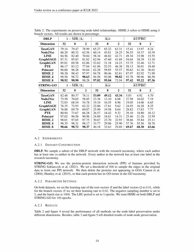
Table 2: The experiments on preserving node-label relationships. HIME k refers to HIME using kbranch vectors. All results are shown in percentage.

DBLP 1−MR/|L| Acc AUPRC

Dimension 32 8 2 32 8 2 32 8 2TaxoGAN 79.14 79.47 78.99 65.27 65.22 63.31 15.41 13.97 8.24Node2Vec 86.20 80.32 62.56 60.14 45.81 24.25 56.55 34.37 10.39

LINE 84.56 82.40 70.84 58.34 46.82 42.71 49.34 33.98 15.55GraphSAGE 87.31 85.83 81.02 62.94 47.60 41.69 54.64 38.39 13.10GraphGAN 85.01 69.58 62.86 52.62 31.18 24.23 53.75 32.46 12.71

PTE 86.17 83.12 77.04 61.96 52.53 46.38 58.13 36.01 18.40Poincare 96.60 96.28 94.64 62.28 59.85 55.57 50.62 41.36 36.62HIME 2 98.30 98.43 97.97 94.78 90.46 82.81 87.97 82.92 71.99HIME 4 98.58 98.72 98.63 94.56 92.08 90.82 93.78 90.96 86.50HIME 8 98.92 98.90 98.28 97.82 95.04 72.94 97.42 95.22 87.36

STRING-GO 1−MR/|L| Acc AUPRC

Dimension 32 8 2 32 8 2 32 8 2TaxoGAN 82.48 80.37 78.11 53.09 49.12 43.34 5.03 4.92 4.70Node2Vec 75.50 70.65 58.85 23.38 13.10 6.08 27.58 16.02 7.19

LINE 72.03 68.54 54.78 19.10 16.55 8.96 19.05 14.06 6.65GraphSAGE 76.35 72.93 62.22 22.06 17.61 9.62 24.93 16.28 8.25GraphGAN 76.88 69.79 60.07 25.90 19.58 8.64 28.82 17.83 7.77

PTE 80.94 73.67 66.28 26.57 18.42 9.32 29.10 18.80 10.12Poincare 97.02 96.56 90.96 24.89 18.61 14.31 25.46 21.26 15.59HIME 2 98.01 97.65 97.75 30.67 23.70 22.93 38.66 35.84 25.11HIME 4 98.35 98.31 98.17 33.77 29.06 25.90 57.76 55.56 38.76HIME 8 98.66 98.72 98.37 40.18 32.63 29.69 69.67 68.30 43.66

A.2 EXPERIMENTS

A.2.1 DATASET CONSTRUCTION

DBLP. We sample a subset of the DBLP network with the research taxonomy, where each authorhas at least one co-author in the network. Every author in the network has at least one label in theresearch taxonomy.

STRING-GO. We use the protein-protein interaction network (PPI) of humans provided bySTRING Szklarczyk et al. (2021). We set a threshold of 800 to sample the edges in the originaldata to form our PPI network. We then delete the proteins not appearing in GOA Camon et al.(2004); Huntley et al. (2015), so that each protein has its GO-terms in the GO taxonomy.

A.2.2 PARAMETER SETTINGS

On both datasets, we set the learning rate of the root vectorsR and the label vectorsQ to 0.01, whilefor the branch vectors B we set their learning rate to 0.02. The negative sampling number is set to5, and the batch size is 1000. The LRU period is set to 5 epochs. We train HIME on both DBLP andSTRING-GO for 100 epochs.

A.2.3 RESULTS

Table 2 and figure 4 reveal the performance of all methods on the node-label preservation underdifferent dimensions. Besides, table 3 and figure 5 tell detailed results of node-node preservation.

14


01-MR/|L| Acc AUPRC

25

50

75

100

125

150

175

200

225

250

275

300

79.165.3

15.4

79.5

65.2

14.0

79.0

63.3

8.2

86.2

60.1 56.6

80.3

45.834.4

62.6

24.2

10.484.6

58.349.3

82.4

46.8

34.0

70.8

42.7

15.587.3

62.954.6

85.8

47.638.4

81.0

41.7

13.1

85.0

52.6 53.8

69.6

31.2 32.5

62.9

24.212.7

86.2

62.0 58.1

83.1

52.5

36.0

77.0

46.4

18.496.6

62.350.6

96.3

59.9

41.4

94.6

55.6

36.6

98.3 94.8 88.0

98.490.5

82.9

98.0

82.8

72.0

98.6 94.6 93.8

98.792.1 91.0

98.6

90.8 86.5

98.9 97.8 97.4

98.9 95.0 95.2

98.3

72.987.4

DBLP

01-MR/|L| Acc AUPRC

25

50

75

100

125

150

175

200

225

250

275

300

82.5

53.1

80.4

49.1

78.1

43.3

75.5

23.4 27.6

70.6

13.1 16.0

58.8

72.0

19.1 19.1

68.5

16.6 14.1

54.8

9.0

76.3

22.1 24.9

72.9

17.6 16.3

62.2

9.6 8.3

76.9

25.9 28.8

69.8

19.6 17.8

60.1

8.6

80.9

26.6 29.1

73.7

18.4 18.8

66.3

9.3 10.1

97.0

24.9 25.5

96.6

18.6 21.3

91.0

14.3 15.6

98.0

30.738.7

97.7

23.7

35.8

97.7

22.9

25.198.4

33.8

57.8

98.3

29.1

55.6

98.2

25.9

38.8

98.7

40.2

69.7

98.7

32.6

68.3

98.4

29.7

43.7

Protein_GO

TaxoGANNode2Vec

LINEGraphSAGE

GraphGANPTE

PoincareHIME_2

HIME_4HIME_8

Figure 4: The experiments on preserving node-label relationships.

A.2.4 THE DISTORTION OF THE HIERARCHY

As shown in figure 6, 7, and 8, with the increase of the branch vector number k, the hierarchystructure of the labels is less preserved. Here we mainly present our understanding of hierarchydistortion caused by multi-vector embedding. Given the total loss function:

Losstotal = Lossnn + Lossll + Lossnl,

We should first figure out which part of the loss function contributes to the preservation of the labelhierarchy most, and then find the reason of the hierarchy distortion.

At first glance, one may first guess that Lossll helps preserving the label hierarchy most, since itdepicts the parent-child relationships among labels. However, by using the taxonomy informationT alone, the machine are not likely to generate a correct tree structure in the Poincare ball, with theroot label embedded close to the origin, while the leaf labels embedded near the border. This can beexplained by the fact that each label in a taxonomy tree with un-directed links can be equally viewedas the root. The un-directed parent-child set S gives no extra information of the true root labels tothe machine.

Since Lossnn is specialized in preserving node-node relationships, Lossnl becomes the only an-swer. Labels in a higher hierarchy level will be frequently updated by the positive node-label

15


Table 3: The experiments on preserving node-node relationships.Dataset DBLPMetric AUPRC AUROC

Dimension 32 8 2 32 8 2TaxoGAN 99.12 98.18 64.34 99.70 99.29 90.67Node2Vec 88.62 73.81 29.16 96.27 90.42 65.18


PTE 88.38 85.45 47.02 96.04 95.07 73.89Poincare 94.42 91.95 81.23 97.52 96.04 89.32HIME 99.56 99.46 98.03 99.93 99.91 99.27Dataset STRING-GOMetric AUPRC AUROC

Dimension 32 8 2 32 8 2TaxoGAN 93.10 85.61 41.83 97.47 93.73 74.90Node2Vec 87.84 79.10 43.10 96.02 89.11 71.01


PTE 89.29 75.49 41.40 97.09 88.78 73.57Poincare 90.51 82.12 69.25 97.01 91.69 85.25HIME 94.04 88.90 85.05 98.09 95.95 94.13

Node2Vec GraphSAGE PTE HIME

AUPRC AUROC0

50

100

150

200

250

300

99.1

99.7

98.2

99.3

64.3 90

.7

88.6 96.3

73.8 90

.429.2

65.2

83.5 93.2

54.3

78.7

26.1

53.2

81.3 90.9

59.1 79

.1

23.4

55.7

99.4

99.9

96.4

99.1

71.1 90

.8

88.4 96.0

85.4 95

.147.0

73.9

94.4

97.5

91.9 96.0

81.2 89

.3

99.6

99.9

99.5

99.9

98.0

99.3

DBLP

AUPRC AUROC0

50

100

150

200

250

300

93.1

97.5

85.6 93

.741.8

74.9

87.8 96.0

79.1 89

.143.1

71.0

76.0 90

.5

58.9

80.0

38.9

65.0

88.6 96.6

77.3 89

.134.0

62.9

93.9

97.9

86.5 95

.2

55.0

82.0

89.3 97.1

75.5 88

.841.4

73.6

90.5

97.0

82.1 91

.7

69.2 85

.2

94.0

98.1

88.9 95

.9

85.1 94

.1

STRING-GO

TaxoGAN LINE GraphGAN Poincare

Figure 5: The experiments on preserving node-node relationships. The different shades of the colorsrepresent the results under dimension 32, 8 and 2 from bottom to top.

pairs, therefore single-vector Poincare embedding will place high-level labels near the center ofthe Poincare ball so as to reduce the overall node-label distances. While low-level labels are pushedaway from the center by negative samples. But when excessive branch vectors are allowed, thenode-label distances call be decreased by updating multiple branch vectors, with labels being lazyand stuck in the middle, as shown in figure 8. Therefore, the hierarchy of the labels will be distorted.To prevent the hierarchy distortion, a small branch vector number is suggested.

16



information retrieval

machine learning approaches

computer visionartificial intelligence

data mining

machine learning

HIME_2

Figure 6: The embedding vectors of the research taxonomy produced by HIME 2.

17



information retrievalmachine learning approaches

computer visionartificial intelligence

data mining

machine learning

HIME_4


18


natural language processinginformation retrieval

machine learning approaches

computer vision

artificial intelligence

data miningmachine learning

HIME_8


19

Documents

MULTI-VECTOR EMBEDDING ON NETWORKS WITH TAXONOMIES