Multi-User MISO forVisible Light Communication

A Degree Thesis submitted to the Faculty of theEscola Tècnica Superior d’Enginyeria de Telecomunicació de Barcelona

Universitat Politècnica de Catalunya

by

Roser Viñals Terrés

In partial fulfillmentof the requirements for the Degree in

Science and Telecommunication Technologies Engineering

Advisors

Josep Vidal ManzanoOlga Muñoz Medina

Adrian Agustín de Dios

Barcelona, September 2016

This thesis is dedicated to my mother,for making me believe that everything is possible.

Multi-User MISO for Visible Light Communication

Abstract

The lighting is going through revolution. The use of Light Emitting Diodes (LEDs) has greatly increasedduring the last few years, meanwhile incandescent and fluorescent lamps have become obsolete. The LEDs,apart from being extremely high energy efficient, are able to switch to different light intensities at very highspeed. This fact, along with the looming crisis of Radio Frequency (RF) spectrum, has given rise to anattractive communication technology known as Visible Light Communication (VLC) that uses the huge license-free spectrum of approximately 400 THz, which is more than 1,000 larger than the RF spectrum. This technologyoffers a novel alternative to RF, enabling the development of wireless communications that make use of existinglighting infrastructure.

This thesis studies multi-user multiple-input single-output (MU-MISO) visible light communications tech-niques for indoor broadcast systems. Particularly, we have proposed a railway wagon as scenario. Transmitters,configured as multiple LED arrays, and multiple users equipped with one single photodetector (PD) are consid-ered. We tackle two relevant challenges in such broadcast systems: how to deal with the multi-user interference(MUI) and how to design the whole system in order to meet the requirement of having a real-valued and positiveVisible Light (VL) signal feeding the LED. Unlike RF counterpart, the VL signal is modulated on light intensityand, consequently, is always positive. This critical constraint imposed by intensity-modulated/direct-detection(IM/DD) systems limits the direct application of the extended theory developed for conventional wireless com-munications. Apart from the non-negativity constraint, we examine the design with individual per-LED opticalpower constraints.

This work presents four coordinated multipoint transmission techniques for MISO transmissions in VLC.Linear precoding schemes such as zero-forcing (ZF) have attracted a lot of interest in RF. Firstly, we considerthe design of the ZF precoder giving special attention to a specific generalized inverse known as pseudo-inverse.Alternatively, a Time Division Multiple Access (TDMA) system is also studied. As neither of the two mentionedprecoders are optimal in terms of sum-rate, we proceed with the design of ZF precoders through an optimizationproblem that maximizes the weighted sum-rate considering both the positivity constraint and the maximumoptical power constraint per-LED. We present two approaches for solving this problem. In the first approach, wefind a closed-form solution to the problem that despite being suboptimal achieves a good trade-off between low-complexity and performance. In the second approach, we rewrite the problem as a standard convex problem andwe find numerically the solution. Finally, we demonstrate the improved performance offered by our approaches.

iii

Multi-User MISO per a Communicacions amb Llum Visible

Resum

La il·luminació està en revolució. L’ús dels LEDs, acrònim anglès de Light Emitting Diodes, ha augmentatconsiderablement durant aquests últims anys, mentre que les bombetes incandescents i fluorescents han quedatobsoletes. Els LEDs, a més de ser extremadament eficients energèticament, són capaços de canviar la intensitatde la llum a alta velocitat. Aquest fet, juntament amb la crisi imminent de l’espectre de Radio Freqüència(RF), ha donat lloc a una atractiva tecnologia coneguda com a Visible Light Communications (VLC) o, encatalà, comunicació amb llum visible. Aquesta tecnologia utilitza l’extens espectre de llum visible no llicenciatd’aproximadament 400 THz, que és més de 1.000 vegades més ampli que l’espectre de RF. VLC és una innovadoraalternativa a la RF, ja que permet desenvolupar comunicacions sense fils que reutilitzen les infraestructuresd’il·luminació ja existents.

Aquesta tesi estudia tècniques de multi-user multiple-input single-output (MU-MISO) per comunicacionsamb llum visible en escenaris interiors com pot ser un vagó de tren. Es consideren transmissors configuratscom múltiples LEDs i múltiples usuaris equipats amb un únic fotodetector. En aquest tipus de sistemes ensenfrontem a dos reptes rellevants: com tractar la interferència multi-usuari i com dissenyar el sistema pertal de complir el requeriment de tenir una senyal real i positiva. Al contrari que en RF, el senyal en llumvisible es modula en intensitat i, per tant, és sempre positiu. Aquest requeriment crític imposat per sistemesintensity-modulated/direct-detection (IM/DD) limita l’aplicació directa de la teoria desenvolupada per sistemesconvencionals de comunicació sense fils. A més d’aquesta restricció de no-negativitat, examinem el disseny ambrestriccions individuals de potència òptica per LED.

Aquest treball presenta quatre tècniques de transmissió multipunt coordinada per transmissions MISO enVLC. Els esquemes de precodificació lineals, com per exemple el forçador de zeros (ZF), han sigut molt popularsen RF. Primer, considerem el disseny d’un precodificador ZF mitjançant un tipus específic d’inversa generalitzadaconeguda com a pseudoinversa. Com a alternativa, s’estudia un sistema Time Division Multiple Access (TDMA).Donat que cap dels dos precodificadors són òptims pel que fa al sum-rate, continuem el nostre estudi ambel disseny de precodificadors ZF mitjançant un problema d’optimització que pretén maximitzar el sum-rateponderat considerant tant la restricció de positivitat com la de potència òptica màxima per LED. Presentemdos plantejaments per solucionar el problema. En el primer, trobem una solució tancada del problema que,tot i ser subòptima, aconsegueix un bon compromís entre complexitat i rendiment. En el segon, reescrivim elproblema inicial com un problema convex estàndard i trobem la solució numèricament. Finalment, demostremla millora en el rendiment que ens proporcionen els nostres precodificadors.

iv

Multi-User MISO para Comunicaciones con Luz Visible

Resumen

La iluminación está en revolución. El uso de los LEDs, acrónimo inglés de Light Emitting Diodes, ha aumen-tado considerablemente durante estos últimos años, mientras que las bombillas incandescentes y fluorescenteshan quedado obsoletas. Los LEDs, a parte de ser extremadamente eficientes energéticamente, son capaces decambiar la intensidad de la luz a alta velocidad. Este hecho, juntamente con la crisis inminente del espectro deradio frecuencia (RF), ha dado lugar a una atractiva tecnología conocida como Visible Light Communications(VLC) o, en castellano, comunicación con luz visible. Esta tecnología utiliza el extenso espectro de luz visibleno licenciado de aproximadamente 400 THz, que es más de 1.000 veces más ancho que el espectro de radiofrecuencia. VLC es una innovadora alternativa a la RF ya que permite desarrollar comunicaciones inalámbricasque reutilizan las infraestructuras de iluminación ya existentes.

Esta tesis estudia técnicas multi-user multiple-input single-output (MU-MISO) para comunicaciones con luzvisible en escenarios interiores como un vagón de tren. Se consideran transmisores, configurados como múltiplesLEDs, y múltiples usuarios equipados con un único fotodetector. En este tipo de sistemas, nos enfrentamos a dosretos relevantes: cómo tratar la interferencia multi-usuario y cómo diseñar el sistema para cumplir el requisito detener una señal real y positiva. Al contrario que en radio frecuencia, la señal de luz visible se modula en intensi-dad y, por tanto, es siempre positiva. Este requisito impuesto por sistemas intensity-modulated/direct-detection(IM/DD) es crítico y limita la aplicación directa de la teoría desarrollada para sistemas convencionales de co-municación inalámbricas. Además de esta restricción de no-negatividad, examinamos el diseño con restriccionesindividuales de potencia óptica por LED.

Este trabajo presenta cuatro técnicas de transmisión multipunto coordinada para transmisiones MISO enVLC. Los esquemas de precodificación lineal, como por ejemplo el forzador de ceros (ZF), han sido muy popularesen RF. Primero, consideramos el diseño del precodificador ZF mediante un tipo específico de inversa generalizadaconocida como pseudoinversa. Como alternativa, se estudia un sistema Time Division Multiple Access (TDMA).Dado que ninguno de los dos precodificadores son óptimos a nivel de sum-rate, procedemos con el diseño deprecodificadores ZF mediante un problema de optimización que pretende maximizar el sum-rate ponderadoconsiderando tanto la restricción de positividad como la potencia óptica máxima por LED. Presentamos dosplanteamientos para solucionar el problema. En el primero, encontramos una solución cerrada que, a pesar deser subóptima, consigue un buen compromiso entre complejidad y rendimiento. En el segundo, reescribimos elproblema inicial como un problema convexo estándar y encontramos la solución numéricamente. Finalmente,demostramos la mejora en el rendimiento proporcionada por nuestros precodificadores.

v

Acknowledgments

I would like to express deepest gratitude to my advisor Prof. Josep Vidal for his full support, motivation,understanding and encouragement throughout this thesis. Additionally, I would also like to thank Olga Muñozand Adrian Agustín for their support and insightful help. Without your guidance and persistence, this thesiswould not have been possible.

To my friends, thanks for making so many ordinary moments, extraordinary. You have been essential duringthese last four years in university.

Lastly, I would like to thank my parents and brothers for encouraging me in all of my pursuits and inspiringme to follow my dreams. Words cannot express what do you mean to me. For all this and much more, thankyou.

vi

List of Acronyms

ACO-OFDM Asymmetrically Clipped Optical OFDM

ADO-OFDM Asymmetrically Clipped DC Biased Optical OFDM

AWGN Additive White Gaussian Noise

BD Block Diagonalization

BER Bit Error Rate

BW Bandwidth

CDF Cumulative Distribution Function

CIR Carrier-to-Interference Ratio

CSI Channel State Information

CSK Color Shift Keying

DC Direct Current

DCO-OFDM DC Biased Optical OFDM

EM Electromagnetic

FET Field Effect Transistor

FOV Field of View

GPS Global Positioning System

IEEE Institute of Electrical and Electronic Engineers

IFFT Inverse Fast Fourier Transform

IM/DD Intensity Modulation / Direct Detection

ISO International Organization for Standardization

ITS Intelligent Transportation System

vii

LED Light-Emitting Diode

Li-Fi Light fidelity

LOS Line-of-sight

LPS Light positioning system

MAC Media Access Control

MIMO Multiple-Input Multiple-Output

MISO Multiple-Input Single-Output

MPAM Multilevel Pulse Amplitude Modulation

MPPM Multi-pulse Pulse Position Modulation

MUI Multi-User Interference

MU-MISO Multi-User Multiple-Input Single-Output

NLOS Non-line-of-sight

O/E Optical-to-electrical

OFDM Orthogonal Frequency Division Multiplexing

OOK On-Off Keying

PAM-DMT Pulse Amplitude Modulated DMT

PD Photodiode

PF Proportional Fairness

PHY Physical layer

PPM Pulse Position Modulation

PSD Power Spectral Distribution

PWN Pulse Width Modulation

RF Radio Frequency

RGB Red-Green-Blue

viii

RX Receiver

SFO-OFDM Spectrally Factorized OFDM

SINR Signal-to-Interference-plus-Noise Ratio

SNR Signal-to-Noise Ratio

s.t. Subject to

SVD Singular Value Decomposition

TDMA Time Division Multiple Access

TX Transmitter

U-OFDM Unipolar OFDM

V2I Vehicle to Infrastructure

V2V Vehicle to Vehicle

VL Visible Light

VLC Visible Light Communication

VLCC Visible Light Communications Consortium

Wi-Fi Wireless Fidelity

ZF Zero-forcing

ix

Notation

x A column vector.

X A matrix.

I The identity matrix.

0 All-zeroes matrix or vector with appropriate dimensions.

tr(X) The trace of X.

diag(x) A diagonal matrix.

(·)H The hermitian (transpose and conjugate) operator.

(·)T The transpose operator.

(·)∗ The conjugate operator.

|·| The absolute value operator.

||·||p The p-norm operator.

⊗ Convolution.

X† The Moore-Penrose pseudo-inverse of X.

X � 0 X is positive semidefinite.

R The field of real numbers.

C The field of complex numbers.

E The mathematical expectation operator.

x

List of Symbols

Symbol MeaningST (λ) Transmitter power spectral distribution functionV (λ) Luminosity functionλH Highest wavelength of the VL spectrumλL Lowest wavelength of the VL spectrum% Maximum luminous efficiency

FT Luminous fluxgt(θ) Luminous intensity

Io Axial intensityθmax Half Beam Angle

n Order of Lambertian emissionΦ1/2 Transmitter semi-angle at half-power.Pt Transmitted optical power,PL Path loss for LOSAr Effective receiver’s areaα Incident angleβ Irradiation angleD Distance between transmitter and receiverPrl Received optical power from the l-th LED

Rf (λ) Spectral response of the optical filterFOV Acceptance angle of the receiverPrTotal

Total received optical powerTs(α) Gain of the optical filterg(α) Gain of the optical concentrator

κ Refractive index of the concentrator.hl,k DC channel gain between the l-th LED and the k-th PD

ρ Reflectivity of a surfaceσ2shot Shot noise variance

σ2thermal Thermal noise variance

σ2 Total noise varianceq Electronic chargeγ ResponsivityB Equivalent noise bandwidth of the PDIB Photocurrent due to background radiation

I2, I3 Noise bandwidth factorsTk Absolute temperature

Cpd Capacitance of the PD per unit areaGol Open-loop voltage gainη FET channel noise

kB Boltzmann’s constantgm FET transconductance

Ps,MPAM Average energy of the normalized MPAM constellationEhor Horizontal illuminance

I0 Center luminous intensityL Number of LED transmittersK Number of PDs or usersPu Received useful optical power tPi Received optical interference poweryk Received optical power samples by user k-thnk Received noise by user k-th

wl,k Precoding weight of LED l-th to user k-th

xi

m Scale factorsk Symbol transmitted to the k-th userbl Bias added in LED l-th

PoptmaxlMaximum optical power transmitted by LED l-th

xii

List of Figures

1.1 Organization of the Degree’s Thesis. . . . . . . . . . . . . . . . . . . . . . . . . . . . . . . . . . . 2

2.1 VLC block diagram. . . . . . . . . . . . . . . . . . . . . . . . . . . . . . . . . . . . . . . . . . . . 42.2 Luminous function, PSD, Lambertian beam distribution and half beam angle of the LED LCW

W5SM; Figure reproduced from [1]. . . . . . . . . . . . . . . . . . . . . . . . . . . . . . . . . . . 52.3 LOS and NLOS propagation model; reproduced from [2]. . . . . . . . . . . . . . . . . . . . . . . 62.4 2-PPM, OOK, 4-PPM and 4-PAM modulations; reproduced from [3]. . . . . . . . . . . . . . . . . 92.5 MPAM constellation. . . . . . . . . . . . . . . . . . . . . . . . . . . . . . . . . . . . . . . . . . . . 9

3.1 LED lights distribution and illuminance achieved. . . . . . . . . . . . . . . . . . . . . . . . . . . . 123.2 Optical power received, SNR, CIR and SINR. . . . . . . . . . . . . . . . . . . . . . . . . . . . . . 12

4.1 Selected point that satisfies the non-negativity and the maximum optical power constraints andachieves the highest SNR. . . . . . . . . . . . . . . . . . . . . . . . . . . . . . . . . . . . . . . . . 15

4.2 BER bound representation (4.22) as a function of SNR for different MPAM modulations usingthe pseudo-inverse of the channel as the precoding matrix. . . . . . . . . . . . . . . . . . . . . . . 16

4.3 Instantaneous transmitted optical power per LED using the pseudo-inverse of the channel as theprecoding matrix. . . . . . . . . . . . . . . . . . . . . . . . . . . . . . . . . . . . . . . . . . . . . . 16

4.4 TDMA system. Disjoint periods of time are allocated to different users. . . . . . . . . . . . . . . 174.5 Feasible points that satisfy the non-negativity and the maximum optical power constraints and

selected value of mk for each slot. . . . . . . . . . . . . . . . . . . . . . . . . . . . . . . . . . . . 184.6 BER bound representation as a function of SNR for different MPAM modulations within the

TDMA slots. . . . . . . . . . . . . . . . . . . . . . . . . . . . . . . . . . . . . . . . . . . . . . . . 194.7 Instantaneous transmitted optical power per LED in each TDMA slot. . . . . . . . . . . . . . . . 194.8 Adaptive algorithms results for the optimal precoding matrix, the suboptimal matrix narrowing

the optical power constraint and without narrowing the optical power constraint. . . . . . . . . . 24

5.1 BER and rate comparison. . . . . . . . . . . . . . . . . . . . . . . . . . . . . . . . . . . . . . . . 255.2 Rate and sum-rate CDF. . . . . . . . . . . . . . . . . . . . . . . . . . . . . . . . . . . . . . . . . . 265.3 Optical power consumption CDF. . . . . . . . . . . . . . . . . . . . . . . . . . . . . . . . . . . . . 275.4 Proportional fair scheduling results. . . . . . . . . . . . . . . . . . . . . . . . . . . . . . . . . . . 29

A.1 Tasks and time planning of the Degree’s Thesis. . . . . . . . . . . . . . . . . . . . . . . . . . . . . 33A.2 Gantt chart of the Degree’s Thesis. . . . . . . . . . . . . . . . . . . . . . . . . . . . . . . . . . . . 33

B.1 LEDs and PDs distribution. . . . . . . . . . . . . . . . . . . . . . . . . . . . . . . . . . . . . . . . 35

xiii

List of Tables

2.1 Differences between VL and RF . . . . . . . . . . . . . . . . . . . . . . . . . . . . . . . . . . . . . 8

B.1 LED and PD parameters . . . . . . . . . . . . . . . . . . . . . . . . . . . . . . . . . . . . . . . . . 34B.2 Noise parameters . . . . . . . . . . . . . . . . . . . . . . . . . . . . . . . . . . . . . . . . . . . . . 34B.3 LEDs and PDs positions . . . . . . . . . . . . . . . . . . . . . . . . . . . . . . . . . . . . . . . . . 34

xiv

List of Algorithms

4.1 Bisection method . . . . . . . . . . . . . . . . . . . . . . . . . . . . . . . . . . . . . . . . . . . . . 225.1 Proportional fair scheduling for TDMA . . . . . . . . . . . . . . . . . . . . . . . . . . . . . . . . 285.2 Proportional fair scheduling for generalized ZF with weighted sum-rate maximization . . . . . . 28C.1 Finding the optimal ZF for maximizing the weighted sum-rate . . . . . . . . . . . . . . . . . . . 38

xv

Contents

Abstract iii

Resum iv

Resumen v

Acknowledgments vi

List of Acronyms ix

Notation x

List of Symbols xii

List of Figures xiii

List of Tables xiv

List of Algorithms xv

1 Introduction 11.1 Project outline . . . . . . . . . . . . . . . . . . . . . . . . . . . . . . . . . . . . . . . . . . . . . . 11.2 Organization . . . . . . . . . . . . . . . . . . . . . . . . . . . . . . . . . . . . . . . . . . . . . . . 1

2 State of Art 32.1 Introduction . . . . . . . . . . . . . . . . . . . . . . . . . . . . . . . . . . . . . . . . . . . . . . . . 32.2 Applications . . . . . . . . . . . . . . . . . . . . . . . . . . . . . . . . . . . . . . . . . . . . . . . . 32.3 VLC components . . . . . . . . . . . . . . . . . . . . . . . . . . . . . . . . . . . . . . . . . . . . . 42.4 Physical layer characteristics . . . . . . . . . . . . . . . . . . . . . . . . . . . . . . . . . . . . . . 42.5 Modulations . . . . . . . . . . . . . . . . . . . . . . . . . . . . . . . . . . . . . . . . . . . . . . . . 82.6 Standard . . . . . . . . . . . . . . . . . . . . . . . . . . . . . . . . . . . . . . . . . . . . . . . . . 9

3 Scenario definition and interference analysis 113.1 Introduction . . . . . . . . . . . . . . . . . . . . . . . . . . . . . . . . . . . . . . . . . . . . . . . . 113.2 Scenario definition . . . . . . . . . . . . . . . . . . . . . . . . . . . . . . . . . . . . . . . . . . . . 11

4 Coordinated Multipoint Transmission techniques for MISO transmissions in VLC 134.1 Introduction . . . . . . . . . . . . . . . . . . . . . . . . . . . . . . . . . . . . . . . . . . . . . . . . 134.2 System model . . . . . . . . . . . . . . . . . . . . . . . . . . . . . . . . . . . . . . . . . . . . . . . 134.3 Zero Forcing precoding with pseudo-inverse . . . . . . . . . . . . . . . . . . . . . . . . . . . . . . 144.4 Time Division Multiple Access . . . . . . . . . . . . . . . . . . . . . . . . . . . . . . . . . . . . . 174.5 Generalized Zero Forcing . . . . . . . . . . . . . . . . . . . . . . . . . . . . . . . . . . . . . . . . . 19

5 System evaluation 255.1 Introduction . . . . . . . . . . . . . . . . . . . . . . . . . . . . . . . . . . . . . . . . . . . . . . . . 255.2 Rate . . . . . . . . . . . . . . . . . . . . . . . . . . . . . . . . . . . . . . . . . . . . . . . . . . . . 255.3 Sum-rate . . . . . . . . . . . . . . . . . . . . . . . . . . . . . . . . . . . . . . . . . . . . . . . . . 265.4 Optical power consumption . . . . . . . . . . . . . . . . . . . . . . . . . . . . . . . . . . . . . . . 265.5 Proportional fair scheduling . . . . . . . . . . . . . . . . . . . . . . . . . . . . . . . . . . . . . . . 27

6 Conclusions and Future Work 306.1 Conclusions . . . . . . . . . . . . . . . . . . . . . . . . . . . . . . . . . . . . . . . . . . . . . . . . 306.2 Future Work . . . . . . . . . . . . . . . . . . . . . . . . . . . . . . . . . . . . . . . . . . . . . . . 30

xvi

References 30

A Work plan 33

B Parameters 34

C Closed-form solution for the suboptimal ZF precoder 36

D Reformulation of the weighted sum-rate maximization for the optimal ZF precoder 39

xvii

1Introduction

1.1 Project outline

1.1.1 Scope and requirementsVisible light communication has the potential to be a key technology in wireless communication systems. Thehigh data speed and energy efficiency, together with the congestion of the radio frequency spectrum, haveincreased the interest from research community and industries. The IEEE 802.11.7 standard [4] has beendeveloped and in review since 2011, and it is believed that this technology will be successfully commercializedover the coming years. However, there are some important challenges that need to be addressed since they areessential to improve high-speed networks using visible light communication.

The purpose of this project is to develop multi-user multiple-input single-output VLC techniques for indoorbroadcast systems. Two main challenges have to be faced in such broadcast systems: how to deal with the multi-user interference and how to design the whole system in order to meet the requirement of having a real-valuedand positive signal.

The project goals can be summarized as follows:

1. Provide a general overview of VLC and its applications.

2. Design of cooperative MU-MISO VLC techniques based on the restrictions of signal positivity and trans-mitted power.

3. Evaluate the precoding schemes performance and compare them in terms of rate, sum-rate and powerconsumption.

4. Evaluate the precoding techniques with proportional fair scheduling.

Thus, the main project requirement is to provide improved MU-MISO VLC techniques through the obtentionof the optimal precoding matrix with two critical constraints: the non-negativity constraint imposed by IM/DDand a maximum optical power emitted per LED. In addition, other suboptimal techniques will be designed andcompared.

1.1.2 BackgroundVisible light communication elicited interest from the Theory and Communications of the Universitat Politècnicade Catalunya and the department decided to open up a new line of research in this topic. Therefore, thisBachelor’s thesis is performed in the framework of the Theory and Communications Department. The initialproject proposal was suggested by the thesis supervisor, Professor Josep Vidal. Adrian Agustín and OlgaMuñoz, also from the Theory and Communications Department, have also provided key feedback and suggestionsregarding the main objectives.

1.2 Organization

1.2.1 Thesis organizationThis Degree’s thesis is organized in six chapters. The first one is the introduction, where the project outline andits organization is explained. In Chapter 2 an overview of VLC and its applications is provided as well as a deepstudy of the physical layer, modulations and standards for VLC. This chapter includes the bases to understandthe rest of the work. Chapter 3 presents the scenario that we are going to take as a model and dimensionsthis scenario to provide illumination and, simultaneously, communication. In Chapter 4, four different MU-MISO schemes are designed. The first two techniques are based on a specific generalized inverse known aspseudo-inverse and a TDMA system. Then, an optimization problem will be addressed in order to obtain theoptimal precoding matrix through the sum-rate maximization and standard convex optimization methods. The

1

problem is going to be solved from two different prespectives leading to two solutions. Chapter 5 evaluates theperformance of the four different MISO schemes proposed in Chapter 4. Furthermore, a scheduling algorithmwill be defined and simulated on the basis of a mobility pattern of the users. Finally, Chapter 6 includes theconclusions and future tasks. Notice that before the list of contents, there are some notation and acronyms tofacilitate the comprehension of the following chapters, whereas at the end of this document there is a list ofreferences used along this work.

In figure 1.1 the different work packages and the organization of the thesis is illustrated.

Figure 1.1: Organization of the Degree’s Thesis.

1.2.2 Work planThe realization of this work lasted four months. By the end of April, the topic of this work was proposedand in May the 2016, the objectives were fixed. In July, in the critical review, we adapted the goals andcontents established initially to the work progress. Appendix A shows the evolution through these months ofthe performed work.

2

2State of Art

2.1 Introduction

The unprecedented increase of data traffic has cast some doubt about if the current RF spectrum will be able toserve the exponential grow of traffic demand in the future. It is predicted that by 2017, every month more than11 exabytes of data traffic will be transferred through mobile networks [5]. To be able to meet this demand,alternatives to RF have attracted a lot of interest from the research community. One of the promising optionsis Visible Light Communication, a technology that uses the non-regulated visible light spectrum and, withoutdoubt, will be crucial over the coming years.

Even though both RF and VL communications use electromagnetic (EM) waves, they have very differentcharacteristics. Among other advantages, unlike RF waves, EM waves in the visible light frequencies are notharmful for the humans and do not interfere with electronic devices. Moreover, due to its high frequency, thelight can not propagate through opaque barriers such as walls and thus, the VLC systems may be securelydeployed with immunity to other cells interference as the signal is confined to the different rooms.

The LEDs, meanwhile, are replacing the incandescent and fluorescent bulbs due to their higher efficiency[6] and longer lifetime. Apart from being widely used in light infrastructures, they have the valuable propertythat they can vary their light intensities at very high speed without the detection by the human visual system,providing a limited bandwidth of about 30−50 MHz. This characteristic is the main reason why the LEDsare suitable to be used as transmitters. Therefore, the LEDs that are already being used to illuminate can,simultaneously, be reused to communicate.

In this chapter, the state of art of this cutting-edge technology will be exposed.

2.2 Applications

VLC is intended to be essential for a lot of applications. In this section three applications will be described:Light Fidelity (Li-Fi), Light positioning system (LPS), and vehicular communication.

Li-Fi

The most famous application of VLC is Li-Fi, a term coined by Harald Haas in 2011 [7]. Li-Fi wireless networkare intended to provide high-speed data while a room is illuminated and it is an attractive alternative towireless fidelity (Wi-Fi). Li-Fi would complement the existing heterogeneous RF wireless networks allowingWi-Fi systems to off-load a significant portion of wireless data traffic. Among other advantages, Li-Fi willprovide much greater speed than Wi-Fi, it is cheaper and can be deployed by reusing the existing lightinginfrastructure. Recently, authors in [8] have reported a data rate of 3 Gbps using VLC.

LPS

One of the most promising applications of visible light communications is indoor positioning. Although theGlobal Positioning System (GPS) is successful for outdoor scenarios, it does not work in indoor environments.Indoor positioning will enable a lot of commercial applications such as indoor navigation for pedestrians insidelarge buildings and location-based services.

There are many proposed indoor positioning solutions based on radio-wave techniques. Indeed, the applica-tion of Wi-Fi for positioning systems has been very popular. However, these solutions achieve less accuracy thanVLC for two reasons. Firstly, they suffer multipath effects and interference from other RF-based technologies.Secondly, the number of LED lights in a building is greater than the number of Wi-Fi Access Points. Anotheradvantage of LPS is the re-use of the current lighting infrastructures which can be translated into substantialcost savings. For all the reasons mentioned above VLC has been identified as the future of indoor localization.

3

Vehicular communication

LEDs are widely employed in traffic lights, signals and street lights. All of these illumination sources could beused to transmit traffic information to cars and pedestrians. Moreover, the vehicles are equipped with headlightsand taillights that could also be used as transmitters. We can distinguish two types of vehicular communications:Vehicle to Infrastructure (V2I) and Vehicle to Vehicle (V2V). The main goal of these communications is to assistdrivers with complying with traffic regulations and making safe decisions. For example, one possible V2V systemcould be a collision warning application that forwards information among vehicles to help identify objects andincidents in the road and prepares the safety protection systems of vehicles when there are unavoidable collisions.

2.3 VLC components

In this section, a general overview of the transmitter and receiver components will be provided.

Transmitter

The key enabling technology for VLC has been the LED. An LED lamp is formed by one or multiple LEDs anda driver circuit which permits to modulate the data throught the control of the LED brightness. Mainly, twodifferent categories of LED have been considered as VLC transmitters.

On the one hand, the blue LED with phosphor is the most commonly used as it is commercially availablewith low cost. It is formed by the combination of a blue LED and a yellow phosphor coating and produceswhite light. Since the phosphor coating has a slow response, it limits the speed in which the LED varies its lightintensity and, therefore, its bandwidth (BW). On the other hand, the Red-Green-Blue (RGB) LED provideshigher bandwidths and data rates. It produces white light by the combination of the three colors. Due to itscomplexity, it has a higher cost. In addition, the RGB LEDs enable Color Shift Keying (CSK) and is verypromising for high data rate applications.

Receiver

Optical receivers for VLC can be divided into two types. The optical non-imaging receiver consists of a singlePD and an optical element such as a optical concentrator or a lens. A PD is a semiconductor-device thatconverts radiation into photo-current, i.e. the received light into current. By contrast, the imaging sensor, alsoreferred as camera sensor, consists of multiple photodiodes and is available in any mobile device with camera.This kind of sensor has a huge drawback: due to its large number of PDs, it is not possible to read the outputof each pixel in parallel and this fact slows down the overall system. Consequently, the non-imaging sensorprovides a higher throughput in comparison to the camera sensor.

In this work, we are going to assume the transmitter to be an LED lamp formed by multiple blue LEDs withyellow phosphor coating and the receiver to be a single PD unless otherwise mentioned specifically. In figure2.3, a generic VLC block diagram is specified.

Figure 2.1: VLC block diagram.

2.4 Physical layer characteristics

This section has been split up into four subsections: the transmitted optical power, path loss and channel model,noise and Signal-to-Noise Ratio (SNR) and, finally, main differences compared to RF.

4

Transmitted optical power

There are two kind of parameters that characterize the LED lights: the photometric parameters that quantifythe light’s interaction with the human eye and the radiometric that measure electromagnetic radiation of light[9]. The luminous flux is a photometric magnitude that measures the total amount of light emitted by an LEDin lumens (lm). It is given by the following integral [10]:

FT = %

ˆ λH

λL

ST (λ)V (λ)dλ [lm] (2.1)

where ST (λ) denotes the Power Spectral Distribution (PSD) function of the LED, V (λ) the luminosity function,λH and λL the highest and the lowest wavelengths of the VL spectrum, i.e. 780 nm and 380 nm, and % is themaximum luminous efficiency, about 683 lm/W. The LED’s PSD represents the power of an LED at differentwavelengths of the spectrum and the luminosity function (V (λ)) represents the average spectral sensitivity ofthe human eye perception of brightness. The luminous efficiency is the ratio of luminous flux to power, measuredin lm/W. In figure 2.2a, the normalized ST (λ) and V (λ) are represented.

(a) Luminosity function (dashed line) representing the humaneye perception of brightness and PSD (solid line) for an LED.

(b) Lambertian radiation pattern and its half beam angle(58º)

Figure 2.2: Luminous function, PSD, Lambertian beam distribution and half beam angle of the LED LCWW5SM; Figure reproduced from [1].

Alternatively to (2.1), the luminous flux is also provided by the following spatial integral:

FT = I0

ˆ θmax

0

2πgt(θ)sinθdθ [lm] (2.2)

where gt(θ) is the luminous intensity, I0 is the axial intensity and θmax is the Half Beam Angle. The luminousintensity indicates the energy flux per a solid angle and it is used for quantifying the brightness of an LED.It is measured in candelas (cd). Most LEDs have a Lambertian beam distribution [11] which means that theluminous intensity distribution is a cosine function. It can be modeled by

gt(θ) = cosn(θ) (2.3)

where n is the order of Lambertian emission given by

n =ln 2

ln(cosΦ1/2)(2.4)

where Φ1/2 is the transmitter semi-angle at half-power. A typical value for a Lambertian transmitter is Φ1/2 =60º. The axial intensity is the luminous intensity at θ = 0º and the half beam angle is the angle in which thelight intensity is half of the axial intensity. In figure 2.2b, the normalized luminous intensity with the axialintensity and the half beam angle is shown.

The transmitted optical power (also known as radiant flux) is a radiometric magnitude that can be calculatedby integrating the PSD over the wavelengths of the visible light [12] leading to the following expression:

Pt =

ˆ λH

λL

St(λ)dλ [W]. (2.5)

In this thesis, we are going to assume that the LEDs have a Lambertian radiation unless otherwise statedspecifically.

5

Path loss and channel model

Authors in [13] modeled the path loss for direct Line-Of-Sight (LOS) as

PL =(n+ 1)Ar

2πD2cosn(β) cos(α) (2.6)

where Ar is the effective receiver’s area, n is the order of the Lambertian source given by (2.4), α and β are theincident angle and irradiation angle, respectively, and D the distance between transmitter and receiver (figure2.3a). The received optical power can be expressed as

Pr = PL

ˆ λH

λL

St(λ)Rf (λ)dλ [W] (2.7)

where Rf (λ) is the spectral response of the optical filter.

(a) LOS link. (b) NLOS link. The signal can bounce several timesbefore reaching the PD.

Figure 2.3: LOS and NLOS propagation model; reproduced from [2].

Normally, a PD will receive light from multiple LEDs. We can obtain the total optical power received bysumming the different contributions of the light beams within the field of view (FOV) of the PD. The FOV isthe acceptance angle of the receiver. For a total of L LEDs

PrTotal=

L∑l=1

Prl [W]. (2.8)

From (2.6), we can provide an expression for the channel. In the channel model we are going to considerthe responses of the receiver’s optical filter and concentrator. The Direct Current (DC) channel gain betweenthe l-th LED and the k-th PD is given by:

hl,k =

{(n+1)Ar

2πD2l,k

cosn(β) cos(α)Ts(α)g(α) 0 ≤ α ≤ FOV

0 α > FOV(2.9)

where Ts(α) is the gain of the optical filter and g(α) the gain of the optical concentrator. For a Lambertiansource, g(α) is given by

g(α) =

{κ2

sin2(FOV )0 ≤ α ≤ FOV

0 α > FOV(2.10)

where κ is the refractive index of the concentrator.Then, we can further express (2.8) as

Prk =

L∑l=1

Ptlhl,k [W]. (2.11)

where hl,k denotes the downlink channel from the l-th LED to the k-th user. It is worthy to mention that noneof this expressions takes the multiple reflexions into consideration (LOS). Hereafter, we are going to present the

6

channel model for a non-line-of-sight (NLOS) scenario. Let ρ be the spectral reflectance, which is the reflectivityof a surface. The receiver power is given by the direct path and by the multiple bounds as follows [14]

Prk =

L∑l=1

Ptlhl,k +

ˆsurface

Pt dhref [W] (2.12)

where dhref is given by

dhref =

{(n+1)Ar

2πD21D

22ρ dAsurface cos

n(β1) cos(α1) cos(β2) cos(α2)Ts(α2)g(α2) 0 ≤ α2 ≤ FOV

0 α2 > FOV(2.13)

where D1 is the distance between an LED and the reflective point, D2 the distance between this reflective pointand the PD and dAsurface the reflective area of small region. Figure 2.3b illustrates the transmitter and receiverpositions and the reflected paths with the respective angles.

As demonstrated in [14], the LOS link accounts for more than 95% of total received optical power. Conse-quently, we will consider the LOS propagation path only.

Please, refer to B.1 where the values of the LED and PD parameters that are going to be used in this workare specified.

Noise and SNR

In an indoor VLC system, three noises prevail: the ambient noise, the thermal noise and the shot noise. Theambient noise is produced by solar radiation or by other artificial illumination sources such as incandescentsand fluorescents bulbs and it is considered a DC interference. Therefore, the receiver reduces the effect ofthis background light by using an electrical high pass filter. By contrast, the shot noise is produced becausethe amount of light emitted by a source (an LED in our case) is not constant and has detectable statisticalfluctuations. The random process of light emission can be modeled using a Poisson distribution resulting thefollowing variance:

σ2shot = 2qγPrB + 2qIBI2B (2.14)

where q is the electronic charge, γ is the responsivity, Pr is the received optical power, B is the equivalent noisebandwidth of the PD, IB is the photocurrent due to background radiation and I2 is a noise bandwidth factor.

The thermal-noise variance is given by

σ2thermal =

8πkBTk

GolCpdAI2B

2 +16π2kBTkη

gmC2

pdA2rI3B

3 (2.15)

where kB is the Boltzmann’s constant, Tk is the absolute temperature, Gol is the open-loop voltage gain, Cpd

is the capacitance of the photodetector per unit area, η is the Field Effect Transistor (FET) channel noise, gmis the FET transconductance and I2 is another noise bandwidth factor.

The total noise is given by the sum of contributions from thermal and shot noise:

σ2 = σ2shot + σ2

thermal. (2.16)

Please, refer to B.2 where the noise parameters that are going to be used in this work are specified.At this point, it is important to remark one striking difference between the optical and electrical power.

Until now, all the powers mentioned were optical powers. However, in order to compute the SNR it is neededa optical-to-electrical conversion (O/E) of the power and this is done through the responsivity γ [A/W]. Let’sfirst define our baseband model

z(t) = γx(t)⊗ h(t) + n(t) (2.17)

where the � symbol denotes convolution.Unlike in RF, x(t) represents the instantaneous transmitted optical power in watts. The average transmitted

optical power is given by the following expression:

Pt = limT→∞

1

2T

T

−T

x(t)dt. (2.18)

Expression (2.18) differs from the one used in RF since instead of x(t) representing powers, x(t) would representamplitude. Therefore, in RF the average power we would have the usual time-average of |x(t)|2. In chapter 4,we are going to limit the maximum instantaneous optical power emitted by each LED to Poptmax = 20 W.

7

The received instantaneous optical power can be written as

y(t) = x(t)⊗ h(t) (2.19)

and the received optical power as

Pr = h·Pt (2.20)

where h is the DC gain between the LED and the PD given by (2.9). By multiplying Pr by γ, we make theO/E conversion obtaining electrical current in Amperes. The electrical SNR is thus given by

SNR =γ2P 2

r

σ2=

γ2(hPt)2

σ2shot + σ2

thermal

. (2.21)

How to overcome this difference between VL and RF is one of the main challenges of this thesis.

Main differences compared to RF

As we have seen, the VLC systems differ from the conventional RF systems in many aspects. In table 2.1, someof this differences will be detailed.

Property RF VL Implications for VL

Spectrum 3 Hz to 3000 GHz. 380 to 780 THz Huge unused free BW.Strictly regulated. Not regulated. Worldwide compatibility.

EM waves Harmful for the humans. Not harmful. Do not Suitable for hospitals,Interfere with electronic interfere with airplanes...devices. electronic devices.

Surface penetration It penetrates walls and other Can not propagate Less coverage.surfaces. Is strongly through opaque Securely deployed.attenuated in water. barriers but propagates Immunity to other

through water. cells interference.Suitable for underwatercommunications.

Channel model The data-carrying signal The signal modulates the x(t) needs tomodulates the complex-valued intensity of the optical be real-valuedbipolar electric field radiated emitter (IM/DD). and positive.by an antenna. Positive channel model

x(t) represents Amplitude Optical power

Average powerproportional to

´|x(t)|2dt

´x(t)dt

Table 2.1: Differences between VL and RF

2.5 Modulations

In this section, various modulations used in VLC will be presented. It is important to highlight that all of thesemodulations will only use the amplitude to encode the data since the signal modulates the intensity of the LED.These modulations are called Intensity Modulated/Direct Detection modulations.

Single-carrier pulse modulations are widely used. The information can be modulated using the amplitude, theduration or the position of the pulse. The On-Off Keying (OOK) modulation, for example, consists of switchingon and off the LED. The data bit 1 is assigned to the on state and the data bit 0 is assigned to off. TheMulti-level Pulse Amplitude Modulation (MPAM) uses different amplitudes to encode the data. Instead, PulseWidth Modulation (PWN) adjusts the pulse duration. The Multi-pulse Pulse Position Modulation (MPPM)uses the pulses position to modulate the data (if only one pulse is used, it is called PPM). Examples for thissingle carrier modulations are shown in figure 2.4.

8

Figure 2.4: 2-PPM, OOK, 4-PPM and 4-PAM modulations; reproduced from [3].

MPAM is the modulation that we are going to apply in this work. In this modulation, the signal is encodedon the amplitude of the pulses. In order to satisfy the non-negativity constraint, a DC-bias should be added.The number of available amplitude levels is denoted by M and the constellation symbols are within the range[−(M − 1), M − 1]. The average energy of the general MPAM constellation is

Ps,MPAM =(−(M − 1))2 + (−(M − 3))2 + ...+ (M − 5)2 + (M − 3)2 + (M − 1)2

M=

M2 − 1

3. (2.22)

However, for future convenience we normalize the MPAM symbols to the range of [−1, 1]. In figure 2.5, thenormalized MPAM constellation is represented. In this case, the average energy is:

Ps,MPAM =M2 − 1

3

1

(M − 1)2=

1

3

(M + 1)

(M − 1). (2.23)

Figure 2.5: MPAM constellation.

Alternatively, multi-carrier modulation such as Orthogonal Frequency Division Multiplexing (OFDM) arealso considered in VLC. Nevertheless, OFDM needs to be adapted in order to have a real-valued and unipolarnon-negative signal. Several approaches have been studied. The most popular are the Asymmetrically ClippedOptical OFDM (ACO-OFDM) [15] and the DC Biased Optical OFDM (DCO-OFDM) [16]. In ACO-OFDM onlythe odd subcarriers are used and the hermitian symmetry is forced. After computing the Inverse Fast FourierTransform (IFFT), the hermitian symmetry leads to real time domain signal and the use of odd subcarriers leadsa time domain asymmetric signal. In this way, the IFFT output has a negative part that is an antisymmetriccopy of the positive part and then, can be clipped at zero without losing any information. In DCO-OFDM, thehermitian symmetry property is also used to get a real ODFM symbol. Unlike ACO-OFDM, all the subcarriersare used and a bias is added to have a positive signal. Other popular multi–carriers modulations are, amongothers, ADO-OFDM [17], which combines DCO-OFDM and ACO-OFDM, U-OFDM [18], SFO-OFDM [19] andPAM-DMT [20].

In section 2.3, a novel type of LED has been presented: the RGB-LED. This kind of LEDs enable amodulation called CSK [21] where the three colored LEDs are used simultaneously to transmit data and thereceiver is able to detect the three components separately. In [22], an improvement of the CSK modulation ispresented by using four LEDs (blue, cyan, yellow and red) instead of three. CSK has been identified as one ofthe most promising modulations.

2.6 StandardIn this section, the Institute of Electrical and Electronic Engineers (IEEE) standard for visible light communi-cation, IEEE 802.15.7 [4], is going to be presented. Other standards had been proposed before by the VisibleLight Communications Consortium (VLCC) in 2007. Nevertheless, it was not until 2011 when the IEEE wroteits standard, the IEEE 802.15.7 that has had a huge impact in VLC. IEEE 802.15.7 includes the physical layer

9

(PHY) and Media Access Control (MAC) design specifications for short range optical wireless communicationsusing visible light.

Among other properties, the standard is capable of providing data rates that allow audio and video multi-media services. It studies the mobility of the visible link, the compatibility with visible-light infrastructures,the impairments due to noise and interference, the health and other environmental effects and, designs a MAClayer that accommodates visible links. It also examines potential applications such as point-to-point commu-nication, secure point-to-Multipoint communication, indoor LBS, Intelligent Transportation System (ITS) andinformation broadcast.

In addition, the standard faces two challenges: flicker mitigation and dimming support. Flicker is caused bythe fluctuation of the brightness of light. This fluctuation, when it is perceived by the visual system, can have anegative effect in humans. To avoid flicker, the changes in light intensity must happen at a rate faster than thehuman eye is able to perceive. A higher frequency than 200 Hz is generally considered safe [23] and, thus, themodulations used should provide a higher rate . On the other hand, the relation between the measured lightand the perceived light is not linear. The standard tries to overcome this non-linear relation ensuring that thecommunication is not affected by the dimming. Different flickering mitigation and dimming support techniquesare deeply studied in IEEE 802.15.7.

The MAC supports three multiple access topologies: peer-to-peer, star configuration and broadcast modeand handles the physical layer management issues. The physical layer, is divided into three types; PHY I, PHYII and PHY III according to the applications.

PHY I is designed for outdoor systems where the data rate requirement is low (achieves rates to the tensto hundreds of kb/s). It uses OOK and PPM and supports concatenated coding with Reed–Solomon andconvolutional coding for forward error correction. PHY II is intended for indoor use with data rates in tensof Mb/s and also uses OOK and PPM. Reed–Solomon coding is also supported for forward error correction.Finally, PHY III is designed for applications with RGB sources. It has similar rates than PHY II and it usesCSK. Again Reed–Solomon coding is also supported.

10

3Scenario definition and interference analysis

3.1 IntroductionVL systems are a preferred solution in areas where the interference with RF technology is an issue such as intrain cabins. In this chapter, the deployment of an optical wireless network within an train cabin is considered.In this section, the scenario will be presented and dimensioned. Afterwards, it will be analyzed in terms ofreceived power, noise and interference.

3.2 Scenario definitionWhether for professional or personal reasons, trains have been for centuries one of the most popular modesof transportation. Every day, thousands of people take a train to go to work, to school and while enjoying afast journey to their destination, they really appreciate enjoying a fast connection to the internet. That is whyan increasing number of train companies are nowadays providing on board Wi-Fi. As alternative to Wi-Fi,we propose to deploy a Li-Fi network. Apart from achieving greater speed, it is cheaper, can be deployed byreusing the existing lighting infrastructure and would not interfere with RF-based technology.

The inside of a standard railway wagon has a size of 18.0m x 3m x 2.5m. Taking the wagon’s size as startingpoint we are going fix the number of LEDs and their position in order to perform the dual function of illuminationand communication.

3.2.1 IlluminanceThe illuminance is a photometric magnitude that measures the total luminous flux incident on a surface, perunit area. It quantifies the brightness of an illuminated surface and it is measured in lux (lx). Authors in [14]modeled the illuminance as

Ehor =I0 cos

n(β) cos(α)

D2, (3.1)

where I0 is the center luminous intensity, α and β are the incident angle and irradiation angle, n is the orderof the Lambertian source given by (2.4) and D the distance between transmitter and receiver. According tothe International Organization for Standardization (ISO), the illuminance required for indoor spaces is 300 to1500 lx. In order to obtain this illuminance, we are going to use 33 LED lighting equipments, each one filledwith 1000 LEDs. The LED Lights are installed at a height of 2.4 m from the floor and distributed as shownin figure 3.1a. The horizontal illuminance, that has been computed with the LED lights listed in table B.1, isrepresented in figure 3.1b. From this figure, the sufficient illuminance, is 300 to 1500 lx by ISO, is obtained inall the places of the wagon.

3.2.2 CommunicationThe LEDs distribution in figure 3.1a is too complex for taking it as a model. For this sake of simplicity, we haveselected L = 12 LEDs of the 33 LED lights to be used to communicate. In figure 3.1a, the LED lights that aregoing to have the dual function of illumination and communication are colored in yellow, meanwhile the onesthat only illuminate are colored in orange.

The user’s terminal distribution is going to be considered a random variable. We are going to use K = 6PDs that can be located in any part of the wagon with a height between 0.5m and 1.5m. From now on, we aregoing to consider the distribution specified in figure B.1 and table B.3 unless mentioned specifically.

Received optical power

We will consider that the total optical received power is composed by the addition of the useful power and theinterference power. The useful power is transmitted by the closest LED to the PD and the interference power

11

Z (

m)

0

0.5

1

1.5

2

2.5

X (m)0

5

10

15

Y (m)

0

0.5

1

1.5

2

2.5

3

Illumination and communication

Illumination

(a) Scenario model. The wagon size is 18.0m x 3m x 2.5m. TheLED lights are placed 2.4m from the floor.

15

10

X (m)

5

00

0.5

1

1.5

Y (m)

2

2.5

400

450

500

750

700

650

600

550

3

Illu

min

an

ce

(lx

)

(b) The distribution of illuminance in the train carriage.

Figure 3.1: LED lights distribution and illuminance achieved.

is the received optical power from the other LEDs. Each PD receives L power contributions given by (2.11). Infigure 3.2a we have represented the instantaneous received power for each PD assuming that the 12 LEDs aretransmitting the maximum optical power (Poptmax = 20W, table B.1).

Users1 2 3 4 5 6

Po

we

r [m

W]

0

0.2

0.4

0.6

0.8

1

1.2

1.4

Total powerUseful powerInterferent power

(a)

Users1 2 3 4 5 6

SN

R [

dB

]

0

10

20

30

40

50

60

70

SNR

(b)

Users

1 2 3 4 5 6

dB

-10

-5

0

5

10

15

20

CIRSINR

(c)

Figure 3.2: Optical power received, SNR, CIR and SINR.

SNR, CIR and SINR

From (2.21) and the received optical power, it is easy to compute the SNR. Let’s now obtain the the Carrier-to-Interference Ratio (CIR) and the Signal-to-Interference-plus-Noise Ratio (SINR) as the following ratios

SNR =γ2P 2

u

σ2(3.2)

CIR =γ2P 2

u

γ2P 2i

=P 2u

P 2i

(3.3)

SINR =γ2P 2

u

σ2 + γ2P 2i

=1

1SNR + 1

CIR

(3.4)

where σ2 is given by (2.16), and Pu and Pi denote the useful optical power and the interference, respectively.In figure 3.2b, the results have been represented. One can appreciate that the SNRs achieved are very high.However, we can readily see that some users are really affected by the interference having SINR bellow 0 dB.

12

4Coordinated Multipoint Transmission techniques

for MISO transmissions in VLC

4.1 IntroductionUsually, several LEDs are employed in a light installation in order to provide enough illumination and this factcan be exploited to create optical MISO communications. The scope of this chapter is designing four differenttechniques for MISO multi-user broadcast transmissions in VLC. Linear precoding schemes have attracted a lotof interest in RF. Particularly, zero-forcing is a simple linear precoding method that decouples the multi-userchannel into multiple independent subchannels [24]. In this chapter, ZF precoding for VLC is first addressedusing a specific generalized inverse known as pseudo-inverse in section 4.3. In addition, a TDMA system isanalyzed in section 4.5. As it is going to be shown, neither of the two mentioned precoders achieve goodresults in terms of sum-rate. Finally, in section 4.4 a ZF precoder will be designed with the goal of maximizingthe weighted sum-rate. The optimization problem will be addressed through two different approaches. Inthe first approach, we will find a suboptimal almost closed-form solution. In the second approach, we willrewrite the problem as a standard convex problem and we will solve it numerically. It is worth noting that thecritical constraints imposed by IM/DD systems limit the direct application of the extended theory developedfor conventional wireless communications.

4.2 System modelWe consider a MU-MISO VLC system consisting of L LEDs and K users equipped with one single PD. Thediscrete-time baseband signal of the MISO multi-user broadcast channel is given by

yk = hTk x+ nk, k = 1, . . . ,K (4.1)

where x ∈ RLx1 are the optical transmitted samples and yk the received optical samples for the k-th user;hk ∈ RLx1 denotes the downlink channel from all the LEDs to the k-th user; and nk denotes the receiver realvalued additive white Gaussian noise with zero mean and variance σ2

k = σ2kthermal

+ σ2kshot

(2.16) of the k-thuser. We assume that the full knowledge of Channel State Information (CSI) is available at the transmitter.The expression (4.1) is equivalent in matrix notation to

y = Hx+ n (4.2)where y ∈ RKx1 , H = [h1,h2, ...,hK ]T ∈ RKxL and n ∈ RKx1 . For convenience, we assume that L ≥ K andthat H is full row-rank. Without loss of generality, we can further express x as

x = mWs+ b (4.3)where W = [w1, ...,wK ] ∈ RLxK denotes the precoding matrix, m is a scale factor of the precoding matrix ands ∈ RKx1 is the information-bearing signal. We consider a MPAM modulation and, as explained in section 2.5,we assume that each of the elements of vector s is normalized to the range of [−1, 1]. Since the VLC systemsuse IM/DD, a bias b = [b1, ..., bL]

T ∈ RLx1 should be added in order to fulfill the non-negativity requirement.This non-negativity constraint can be expressed as

(Non-negativity): xl = m

K∑k=1

wl,ksk + bl ≥ 0 →K∑

k=1

wl,ksk ≥ −blm

, l = 1, . . . , L. (4.4)

Taking the worst case, i.e. when the right size of the inequality is minimal (wl,ksk = −|wl,k| ∀k, l), theprecoding weights have to be chosen in such a way that

K∑k=1

|wl,k| ≤blm, l = 1, . . . , L. (4.5)

13

On the other hand, traditionally, the transmitters are designed under the assumption of a total powerconstraint. However, in this thesis it is considered a more realistic scenario where individual per-LED constraintsare imposed. The LEDs are going to be placed geographically separated and, consequently, each transmittershould have its own optical power restriction. The power constraints of a LED is always given by optical power,never by electrical power. Without loss of generality, we assume that it is the same for all the LEDs. Then, theinstantaneous transmitted optical power must also ensure that

(Optical power constraint): xl = m

K∑k=1

wl,ksk + bl ≤ Poptmaxl, l = 1, . . . , L (4.6)

where Poptmaxlis the maximum instantaneous optical power for the l-th LED. Again, taking the worst case that

is given when wl,ksk = |wl,k|, the inequality (4.6) leads to

K∑k=1

|wl,k| ≤Poptmax − bl

m, l = 1, . . . , L. (4.7)

Regarding the SNR, if we combine (4.2) and (4.3), we obtain that

y = mHWs+Hb (4.8)

where Hb is the so-called DC component. We assume CSI in reception and therefore, the receiver can easilyestimate the DC component and remove it. In section 2.4, we have given a general expression for the SNR.After removing the DC component, the electrical SNR (2.21) of the k-th user can be particularized to:

SNR =γ2m2|hT

k wk |2Ps,MPAM

σ2k

(4.9)

where Ps,MPAM is the modulation power given by (2.23) and γ is the responsivity. The noise variance σ2k is

given by the contribution of the thermal and shot noise. As shown in (2.15), the thermal noise is independentof the received optical power whereas the shot noise is not (2.14). The average optical power received by thek-th user is:

E{yk} = E{mhTkwksk + hT

k b} = hTk b. (4.10)

Then, the shot noise of the k-th user can be particularized leading to the following expression:

σ2kshot

= 2qγykB + 2qIBI2B = 2qγ(hTk b)B + 2qIBI2B. (4.11)

From [25], it can be asserted that for a MPAM the exact Bit Error Rate (BER) expression is given by

BERMPAM(SNR) =1

log2 M

(1− 1

M

)erfc

(√1.5SNRM2 − 1

). (4.12)

This expression can be approximated using the Chernoff upper bound, leading to

BERMPAM(SNR) ≤ 0.1 exp

[−1.5SNRM2 − 1

](4.13)

that combined with (4.9) gives rise the following BER bound:

BERMPAM(SNR) ≤ 0.1 exp

[−1.5γ2m2|hT

k wk |2Ps,MPAM

σ2k(M

2 − 1)

]. (4.14)

4.3 Zero Forcing precoding with pseudo-inverse

4.3.1 Eliminating the Multi-user Interference

The use of generalized inverse for precoding matrices is widely accepted. The pseudo-inverse is a specificgeneralized inverse that satisfies that, being A ∈ CKxL any full-rank matrix, its pseudo-inverse A† ∈ CLxK

satisfies that AA† = I where A† = AH (AAH )−1. Taking this definition as starting point, it is easy to realizethat if we take W = H†, we accomplish the ZF objective of having multiple independent sub-channels since

y = Hx+ n = H(mH†s+ b) + n = ms+Hb+ n. (4.15)

14

4.3.2 Fulfilling the constraints

The inequalities (4.5) and (4.7) define a possible set of values for m and b that satisfy both constraints. Thesevalues of m and b satisfying the problem constraints are called feasible values of m and b. For the scenariodefined in chapter 3, the constraints on one single LED define the area shown in figure 4.1a. The selected pairof m and bl is the one that achieves the highest SNR. In (4.9), it is shown that the squared value of the scalefactor appears in the numerator of the SNR. Furthermore, in the denominator they appear both, m and b, inthe shot noise term (4.11). In figure 4.1b, the SNR has been plotted for the feasible pairs of m and bl assumingM = 2. From this figure, it can be observed that the maximum SNR coincides with the maximum value of mwithin the colored area and the respective bl, i.e. the intersection between the constraints (4.5) and (4.7):

Poptmaxl− bl

m=

blm

⇒ bl =Poptmaxl

2(4.16)

Note that Poptmaxlis the same for all the LEDs and, consequently, bl is also the same ∀l. It will be denoted as

b. Thus, we only have two design parameters, m and b, that need to, on the one hand, maximize the SNR and,on the other, meet all the requirements of the different LEDs. Substituting the value of b in (4.5) and (4.7), anunique constraint has to be satisfied:

K∑k=1

|wl,k| ≤Poptmax

2m, l = 1, . . . , L (4.17)

This inequality is satisfied when the most restrictive case is considered, i.e. when the right part of the inequation(4.17) is maximal, leading to the following simplification[

K∑k=1

|wl,k|

]max

l

≤ Poptmax

2m(4.18)

or, equivalently,

m ≤ Poptmax

2[∑K

k=1 |wl,k|]max

l

(4.19)

As stated before, the maximum SNR is achieved with the maximum value of the scale factor. From (4.19),we can deduce that the value of the scale factor is

m =Poptmax

2[∑K

k=1 |wl,k|]max

l

. (4.20)

(a) Feasible points that satisfy the non-negativity and the max-imum optical power per-LED constraints.

(b) SNR obtained for the pairs of m and b that guarantee the non-negativity and the maximum optical power per-LED constraints.

Figure 4.1: Selected point that satisfies the non-negativity and the maximum optical power constraints andachieves the highest SNR.

15

4.3.3 PerformanceBER

The electrical SNR in (4.9) using the precoding matrix as the pseudo-inverse of the channel can be particularizedto:

SNR =γ2m2Ps,MPAM

σ2k

(4.21)

and, consequently, the BER bound in (4.14) can be simplified to

BERMPAM(SNR) ≤ 0.1 exp

[−1.5γ2m2Ps,MPAM

σ2k(M

2 − 1)

]. (4.22)

From (4.22), we can assure that the BER depends on both the selected M and the received SNR. Thus, forthe scenario defined in chapter 3, we can obtain, for a specific constellation, which is the BER achieved by eachuser depending on the electrical received SNR of that user. In figure 4.2, we have plot, on the one hand, theBER in function of the SNR (4.13) for different constellation sizes, each one in a different color. On the otherhand, for each M , we have represented the received SNR of each user and the respective BER. In figure 4.2,each user has a different marker assigned and the marker color reflects the constellation size. It is worthy tomention that each user has a slightly different SNR due to the fact that the shot noise given by (4.11) dependsdirectly on the average optical power received which, in turn, depends on the DC component, hT

k b.

Transmitted optical power

The instantaneous emitted optical power by LED is given by (4.6) and it is represented in figure 4.3 for thescenario defined in chapter 3 with a 2-PAM. One can appreciate that any LED achieves the maximum availablepower because the system design has considered the worst case by taking the absolute value of the weights in(4.5) and (4.7).

SNR

100

101

102

103

104

BE

R

10-10

10-8

10-6

10-4

10-2

100

Maximum BER

M=2M=4M=8M=16M=32M=64M=128M=256User1User2User3User4User5User6

Figure 4.2: BER bound representation (4.22) asa function of SNR for different MPAM modula-tions using the pseudo-inverse of the channel asthe precoding matrix.

LED1 2 3 4 5 6 7 8 9 10 11 12

Tra

nsm

itte

d o

ptical pow

er

by L

ED

[W

]

0

2

4

6

8

10

12

14

Figure 4.3: Instantaneous transmitted opticalpower per LED using the pseudo-inverse of thechannel as the precoding matrix.

4.3.4 Adaptive schemeIn this section, we examine an adaptive modulation scheme where the data rate, transmitted power and con-stellation size are varied to obtain a BER under 10−6 subject to the constraints defined in section 4.3.2. Theobjective of the adaptive modulation is a real-time balancing of the constellation size in order to always achiev-ing a BER under the target. The adaptive scheme takes advantage of the time-varying nature of the channel toobtain the modulation which allows the highest rate defined as r = log2 M [bps/Hz] guaranteeing the link qualityrequired. Furthermore, it allows to transmit at high speed under favorable channel conditions and reduce therate when the conditions are degraded.

From equation (4.22) we have obtained an upper-bound for the BER and we have been able to represent theBER achieved for each user with the available modulations. In figure 4.2, we have represented the users’ BER andSNR when they use each constellation. In this particular case, we can clearly state that the maximum modulationthat achieves the target BER is 8-PAM for all the users (all the markers that represent the different users’ BER

16

and SNR are bellow target BER in the orange plot). Consequently, the achieved rate is r = log2 8 = 3 [bps/Hz].Of course, if we took MPAM constellations with less symbols (M = 2 or M = 4) we would also get a BER underthe target although less rate will be achieved. It is worth noting that different users might have a different ratesince they do not have exactly the same SNR and, consequently, they have different BERs. Nevertheless, inthis example all the users achieve the same rate. In chapter 5, this adaptive scheme will be applied to severalrealizations of the channel in order to evaluate its performance.

4.4 Time Division Multiple Access

4.4.1 Eliminating the Multiuser InterferenceTDMA is a multiple access technique where time slots are assigned to the users. In this way, disjoint periodsof time are allocated to different users for either transmission or reception without interference (figure 4.4).Considering the downlink of our system, the array of LEDs transmits in each slot to a different user. For thesake of simplicity, we have considered that each slot has the same length. In the slot assigned to the k-th user,the signal received is:

yk = hTk xk + nk = hT

k (mkwksk + bk ) + nk (4.23)

where yk denotes the received signal for the k-th user, hk ∈ RLx1 the downlink channel from all the LEDs tothe k-th user, mk the scale factor, wk = [w1,k, ..., wL,k]

T ∈ RLx1 the precoding vector of the k-th user, sk thesymbol associated to the k-th user, bk ∈ RLx1 the bias component and nk the Additive White Gaussian Noise(AWGN).

The precoding vector should maximize the SNR given by

SNR =γ2m2

k|hTk wk |2Ps,MPAM

σ2k

. (4.24)

From (4.24), wk has to be chosen in such a way that the product |hTk wk |2 is maximized. This is fulfilled

when wk = αkhk , that is nothing less than the well-known matched filter in transmission. In order to keep thenotation as simple as possible, we consider that the αk factor is already included in mk.

Figure 4.4: TDMA system. Disjoint periods of time are allocated to different users.

4.4.2 Fulfilling the constraintsThe constraints in TDMA are the same as in section 4.3.2: the non-negativity and the maximum optical powerper LED constraints. Similarly to the previous case, the instantaneous transmitted optical power for the slotk-th must ensure that

(Non-negativity): xl,k = mkwl,ksk + bl,k ≥ 0, l = 1, . . . , L. (4.25)

From the inequality (4.25) and assuming the worst case, we can conclude that the precoding weights for thek-th slot have to be chosen in such a way that

|wl,k| ≤bl,kmk

, l = 1, . . . , L. (4.26)

The instantaneous transmitted optical power must also ensure that

17

(Optical power constraint): xl,k = mkwl,ksk + bl ≤ Poptmax , l = 1, . . . , L (4.27)

or, equivalently,

|wl,k| ≤Poptmax − bl,k

mk, l = 1, . . . , L. (4.28)

For each slot, the inequalities (4.26) and (4.28) define a possible set of values for mk and bk that satisfy bothconstraints. For the same reason explained in the pseudo-inverse scheme, the bias bl,k is always bl,k =

Poptmax

2 .Therefore, the bias added in each LED for each slot is always the same and it will be denoted as b. Moreover,the pair of mk and b selected is the one that allows the highest SNR and it is given by the intersection betweenthe two constraints. Nevertheless, although the bias does not vary, the scale factor can be different for eachslot. Thus, the expressions (4.26) and (4.28) can be narrowed to:

|wl,k|maxl

≤ Poptmax

2mk(4.29)

whose intersection provide the value of the scale factor: mk =Poptmax

2|wl,k|maxl

∀k. On the bases of the matched filter

and the two constraints, in figure 4.5 the different values selected of mk for each slot are illustrated.

Figure 4.5: Feasible points that satisfy the non-negativity and the maximum optical power constraints andselected value of mk for each slot.

4.4.3 Performance

BER

Using the BER bound given in (4.13) and combining it with (4.24), the BER can be approximated to

BERMPAM(SNR) ≤ 0.1 exp

[−1.5γ2m2

k|hTk wk |2Ps,MPAM

σ2k(M

2 − 1)

]. (4.30)

Likewise the procedure followed in the pseudo-inverse, we can plot the BER in function of the SNR for eachslot (figure 4.6). The colored lines represent the BER bounds given by (4.13) for different constellation sizesand the markers, the electrical SNRs and the respective BERs of the user served in each slot when they usethat constellation.

18

SNR

100

105

BE

R

10-20

10-15

10-10

10-5

100

TDMA: User 1

SNR

100

105

10-20

10-15

10-10

10-5

100

TDMA: User 2

SNR

100

105

10-20

10-15

10-10

10-5

100

TDMA: User 3

SNR

100

105

10-20

10-15

10-10

10-5

100

TDMA: User 4

SNR

100

105

10-20

10-15

10-10

10-5

100

TDMA: User 5

SNR

100

105

10-20

10-15

10-10

10-5

100

TDMA: User 6

M=2M=4M=8M=16M=32M=64M=128M=256Achieved BER

Figure 4.6: BER bound representation as a function of SNR for different MPAM modulations within theTDMA slots.

LED1 2 3 4 5 6 7 8 9 101112

Tra

nsm

itte

d o

ptica

l p

ow

er

by L

ED

[W

]

0

2

4

6

8

10

12

14

16

18

20

LED1 2 3 4 5 6 7 8 9 101112

0

1

2

3

4

5

6

7

8

9

10

LED1 2 3 4 5 6 7 8 9 101112

0

1

2

3

4

5

6

7

8

9

10

LED1 2 3 4 5 6 7 8 9 101112

0

2

4

6

8

10

12

14

16

18

20

LED1 2 3 4 5 6 7 8 9 101112

0

1

2

3

4

5

6

7

8

9

10

LED1 2 3 4 5 6 7 8 9 101112

0

2

4

6

8

10

12

14

16

18

20

Figure 4.7: Instantaneous transmitted optical power per LED in each TDMA slot.

Transmitted optical power

The emitted optical power is provided by (4.27) and illustrated in figure 4.7 considering a 2-PAM. For the samereasons already explained in 4.3.3, not all the LEDs use the maximum available power.

4.4.4 Adaptive algorithm

As in section 4.3.4, we design an adaptive modulation scheme where there is real-time balancing of the constel-lation size in order to always achieve the highest rate and a BER under the maximum of 10−6. In contrast withthe pseudo-inverse, the users only transmit in one time slot and the data rate is r = 1

K log2 M [bps/Hz] whereK is the total number of users.

For the specific case of figure 4.6, for the first and second user the M selected would be 128 or, in orderwords, r = 7/6 [bps/Hz] . Instead, for the fifth user the M would be 64 and for the rest of the users would be32, or, analogously, r = 1 [bps/Hz] and r = 5/6 [bps/Hz] . The constellations size selected are those that ensurethe target BER. Note that the intrinsic orthogonalization of TDMA allows us to design a precoder that givesthe maximum SNR and, therefore, the modulation can be much higher than in ZF. However, since each usertransmits only in certain time periods, this fact is not translated into a higher rate. Instead, in most cases, therate is lower than in the previous scheme.

4.5 Generalized Zero Forcing

4.5.1 Introduction

This section offers a deep study of a ZF precoder design to maximize the weighted sum-rate of all users subjectto per-LED optical power constraints. Other design criteria such as minimizing the total power consumptionor the time delay could have been taken. Nevertheless, we have considered that the user’s rate is a priorityin VLC systems. In [26, 27] the design is formulated in a Multiple-Input Multiple-Output (MIMO) broadcastwireless channel. However, these results can not be directly applied in VLC since two critical problems have tobe faced that affects the overall performance: the non-negative constraint of the signal feeding each LED andthe fact that we need to deal with optical power instead of electrical power.

There have been several studies on MU-MISO VLC. In [28], a Block Diagonalization (BD) system for VLChas been studied without taking into consideration the positivity constraint. In [29], a MU-MISO VLC forindoor broadcast system is studied under the constraint of positivity but without maximum power constraint.

19

The weighted sum-rate maximization that they propose leads to a non-convex problem and, therefore, they cannot obtain an exact solution and they confine to a lower-bound for the sum-rate.

In this section, we focus on the maximization of the sum-rate considering both the positivity constraint andthe maximum optical power constraint. To solve this problem we resort to convex optimization techniques. Wewill present two approaches for solving this problem. In the first approach, we will focus on finding an almostclosed-form solution to the problem. Although the solution found is suboptimal (therefore the performanceis worse compared with the second approach), the benefit in this case is the lower complexity. Then, we willdescribe a different approach to solve the problem where we will find numerically the solution. To that end, wewill describe how the the problem can be written as a standard convex problem, that can be solved numericallyusing available software such as those in the optimization toolbox of Matlab (we will actually use directly theconstrained optimization function fmincon in such toolbox [30]). Our contribution is therefore, finding how theproblem can be stated in a standard convex form.

4.5.2 Suboptimal Zero Forcing scheme for maximizing the weighted sum-rate

As starting point, we are going to use the BER upper-bound from (4.14). From equation (2.23), Ps,MPAM =13(M+1)(M−1) , we can observe that if M ≫ 1, Ps,MPAM can be approximated by 1/3. For constellation sizes equal

or greater than M = 8, this approximation leads to a relative error bellow 0.29%. Basing on this statement andconsidering m = 1, the BER bound can approximated by

BERMPAM(SNR) ≤ 0.1 exp

[−1.5γ2|hT

k wk |21/3σ2k(M

2 − 1)

]. (4.31)

Since M = 2r, (4.31) leads to the following rate lower-bound:

r ≥ 1

2log2

(1 + c′|hT

k wk |2)

(4.32)

where c′ = 12

γ2

σ2 log(

0.1BERMPAM

) . Denoting Sk , wkwTk , we can further express (4.32) as

r ≥ 1

2log2

(1 + c′hT

k Skhk

). (4.33)

Remark 4.1. The noise variance is the sum of contributions from thermal and shot noise. The shot noise(4.11) depends on the optical power received, whereas the thermal noise is considered independent (2.15).For convenience, we have assumed that the noise variance is the same for all the users and is given by thethermal noise and the shot noise term that is independent to the average optical received power (σ2

kshot=

2qγ(hTk b)B + 2qIBI2B ≈ 2qIBI2B).

Once we have found the bound for the rate, the precoding matrix needs to satisfy a set of per-LED constraints.On the one hand, the non-negativity constraint forces that

(Non-negativity): xl =

K∑k=1

wl,ksk + bl ≥ 0, l = 1, . . . , L. (4.34)

To fulfill (4.34) for all the cases (i.e. all the possible values of the symbol), the following conditions must befulfilled

K∑k=1

|wl,k| ≤ bl, l = 1, . . . , L. (4.35)

On the other hand, the maximum optical power constraint forces that

(Optical power constraint): xl =

K∑k=1

wl,ksk + bl ≤ Poptmax , l = 1, . . . , L. (4.36)

Again, to satisfy the restrictions in (4.36) for all the possible values of the symbol, the following conditions mustbe fulfilled

K∑k=1

|wl,k| ≤ Poptmax − bl, l = 1, . . . , L. (4.37)

Note that the constraints (4.35) and (4.37) can be expressed as a single constraint

20

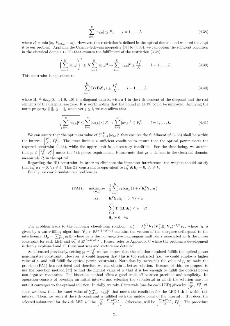
K∑k=1

|wl,k| ≤ Pl, l = 1, . . . , L (4.38)

where Pl = min (bl, Poptmax − bl). However, this restriction is defined in the optical domain and we need to adaptit to our problem. Applying the Cauchy–Schwarz inequality [31] to (4.38), we can obtain the sufficient conditionin the electrical domain (4.39) that ensures the fulfillment of the restriction (4.38).(

K∑k=1

|wl,k|

)2

≤ K

K∑k=1

|wl,k|2 →K∑

k=1

|wl,k|2 ≤ P 2l

K, l = 1, . . . , L. (4.39)

This constraint is equivalent to:

K∑k=1

Tr (BlSk ) ≤P 2l

K, l = 1, . . . , L (4.40)

where Bl , diag(0, ..., 1, 0, ...0) is a diagonal matrix, with a 1 in the l-th element of the diagonal and the restelements of the diagonal are zero. It is worth noting that the bound in (4.39) could be improved. Applying thenorm property ||·||i ≤ ||·||j whenever j ≤ i, we can affirm that√√√√ K∑

k=1

|wl,k|2 ≤K∑

k=1

|wl,k| ≤ Pl →K∑

k=1

|wl,k|2 ≤ P 2l , l = 1, . . . , L. (4.41)

We can assure that the optimum value of∑K

k=1 |wl,k|2 that ensures the fulfillment of (4.38) shall be withinthe interval

[P 2

l

K , P 2l

]. The lower limit is a sufficient condition to ensure that the optical power meets the

required constraint (4.38), while the upper limit is a necessary condition. For the time being, we assumethat pl ∈

[P 2

l

K , P 2l

]meets the l-th power requirement. Please note that pl is defined in the electrical domain,

meanwhile Pl in the optical.Regarding the BD constraint, in order to eliminate the inter-user interference, the weights should satisfy

that hTj wk = 0, ∀j 6= k. This ZF constraint is equivalent to hT

j Skhj = 0, ∀j 6= k.Finally, we can formulate our problem as

(PA1) : maximize{wk}

1

2

K∑k=1

uk log2(1 + c′hT

k Skhk

)s.t. hT

j Skhj = 0, ∀j 6= k

K∑k=1

Tr (BlSk ) ≤ pl ∀l

Sk � 0 ∀k

The problem leads to the following closed-form solution: w∗k = λ

1/2k Vk(V

Tk BµVk)

−1/2υk, where λk isgiven by a water-filling algorithm, Vk ∈ RLx(L−K+1) contains the vectors of the subspace orthogonal to theinterference, Bµ =

∑Ll=1 µlBl where µl is the non-negative Lagrangian multipliers associated with the power

constraint for each LED and υTk ∈ R(L−K+1)x1. Please, refer to Appendix C where the problem’s development

is deeply explained and all these matrices and vectors are detailed.As discussed previously, setting pl =

P 2l

K we can ensure that the solution obtained fulfills the optical powernon-negative constraint. However, it could happen that this is too restricted (i.e. we could employ a highervalue of pl and still fulfill the optical power constraint). Note that by increasing the value of pl we make theproblem (PA1) less restricted and therefore we can obtain a better solution. Because of this, we propose touse the bisection method [32] to find the highest value of pl that it is low enough to fulfill the optical powernon-negative constraint. The bisection method offers a good trade-off between precision and simplicity. Itsoperation consists of bisecting an initial interval and selecting the subinterval in which the solution must lieuntil it converges to the optimal solution. Initially, we take L intervals (one for each LED) given by

[P 2

l

K , P 2l

]∀l,

since we know that the exact value of∑K

k=1 |wl,k|2 that meets the condition for the LED l-th is within thisinterval. Then, we verify if the l-th constraint is fulfilled with the middle point of the interval l. If it does, theselected subinterval for the l-th LED will be

[P 2

l

K ,P 2

l +P2l /K

2

]. Otherwise, will be

[P 2

l +P2l /K

2 , P 2l

]. The procedure

21

is repeated until the convergence providing the optimum pl ∀l. It can be readily seen that each LED mightachieve a different value of pl.

Algorithm 4.1 Bisection methodgiven p∗l ≤ al , p∗l ≥ bl, tolerance ε > 0.repeat

1. x := (a+ b)/2.

2. Solve the concave problem (PA1) with pl = xl.

3. if∑K

k=1 |wl,k| ≤ Pl, l = 1, . . . , L , al := xl; else bl := xl.

until a− b ≤ ε

4.5.3 Optimal Zero Forcing scheme for maximizing the weighted sum-rate

Coming back to (4.14), substituting the modulation power expression (2.23), Ps,MPAM = 13(M+1)(M−1) , and consid-

ering m = 1, the BER bound can be further expressed as

BERMPAM(SNR) ≤ 0.1 exp

[− γ2|hT

k wk |2

2σ2k(M − 1)2

]. (4.42)

Since M = 2r, (4.42) leads to the following rate lower-bound:

r ≥ log2(1 + c|hT

k wk |)

(4.43)

where c = γ

σ

√2log

(0.1

BERMPAM

) .

The precoding matrix should satisfy the non-negativity and optical power constraints given by (4.38). Wecan rewrite this constraint as

K∑k=1

|wl,k| ≤ min (bl, Poptmax − bl) , l = 1, . . . , L (4.44)

that can be expressed as∑K

k=1 |jTl wk| ≤ min (bl, Poptmax − bl) where jl , (0, ..., 0, 1, 0, ..., 0)

T contains a 1 inthe l-th position, while the rest of elements are zero.

Finally, in addition to these constraints, we consider the ZF precoding scheme which eliminates the inter-userinterference, i.e. hT

j wk = 0, ∀j 6= k.We are now ready to formulate the weighted sum-rate maximization problem with the ZF precoding and

per-LED power constraints as follows:

(PB1) : maximize{wk,bl}

K∑k=1

uk log2(1 + c |hT

k wk |)

s.t. hTj wk = 0, ∀j 6= k

K∑k=1

|jTl wk| ≤ min (bl, Poptmax − bl) , ∀l

where uk is the rate weight for the k-th user. Without loss of optimality, we can add the restriction hTkwk ≥

0 ∀k. If the optimal solution of (PB1) were wk such that hTkwk ≤ 0, we could change the sign of wk, i.e.

wk = −wk , in order to satisfy hTk wk ≥ 0. After changing the weights sign, the restrictions would continue

to be met and the objective function would not be penalized. With this new restriction we can change theobjective function leading to a concave problem (we are maximizing). Thus we rewrite the problem as follows:

22

(PB2) : maximize{wk,bl}

K∑k=1

uk log2(1 + chT

k wk

)s.t. hT

j wk = 0, ∀j 6= k

K∑k=1

|jTl wk| ≤ min (bl, Poptmax − bl) , ∀l

hTk wk ≥ 0, ∀k.

(PB2) can be reduced to the following equivalent problem:

(PB3) : maximize{qk,bl}

K∑k=1

uk log2

(1 + chT

k Vkqk

)s.t.

K∑k=1

|jTl Vkqk| ≤ min (bl, Poptmax − bl) , ∀l

hTk Vkqk ≥ 0, ∀k

where Vk ∈ RLx(L−K+1) contains the vectors of the subspace orthogonal to the interference, i.e. hTj Vk = 0, ∀j 6=

k and qk ∈ R(L−K+1)x1 allows wk to be a linear combination of these orthogonal vectors, i.e. wk = Vkqk .

Proof. Please refer to Appendix D.

Problem (PB3) is a concave problem as the objective function is concave on the optimization variables (weare maximizing) and the constraints are either convex (note that any norm is convex) or linear. Being problem(PB3) concave it can be solved numerically using standard optimization tools with an affordable computationalcomplexity while guaranteeing that the optimum solution is found, along with the values of the variables (i.e.optimal values for each user’s precoder and bias component per LED) achieving the maximum of the costfunction. In particular, we have used the fmincon function of the convex optimization toolbox of Matlab tofind the solution of problem (PB3), i.e. the optimal BD precoding vectors for each user and the optimalbias component bl for each LED. For the purpose of exposition, we are going to call optimal ZF precoder theprecoding matrix so obtained.

4.5.4 Adaptive algorithm

In this section, adaptive modulation algorithms are studied based on the two proposed schemes presented in4.5.3. As it has been done for the pseudo-inverse and for TDMA, the constellation size is modified in order toachieve the highest rate and a BER under the maximum of 10−6. The data rate, in this case, is the same as forthe pseudo-inverse r = log2 M [bps/Hz].

In figure 4.8a, the BER is represented for three different cases: the optimal ZF precoder (red), the suboptimalZF precoder with the narrowed power restriction (cyan) and, the suboptimal ZF precoder without narrowingthe power constraint (blue) . For the purpose of simplification, we have assumed that the rate’s weights uk

are 1. Each marker represents the achieved SNR by an user and the respective BER when the user use thedifferent constellations. In 4.8b, the different rates achieved are illustrated and in 4.8c the sum-rate. Thesetwo plots suggest that the optimal and the suboptimal precoding matrix with the narrowed power constraintconstitute an improvement compared to the suboptimal ZF precoder without narrowing the power constraintsince they achieve higher rates and sum-rate. We denote the suboptimal precoding matrix with the narrowedpower constraint as suboptimal precoder 1 and the suboptimal ZF precoder without narrowing the optical powerconstraints as suboptimal precoder 2. The rates in 4.8b are obtained as follows.

Firstly, the higher constellation sizes are considered. In figure 4.8a, with M = 64 two users with the optimaland the suboptimal precoder 1 achieve a BER under the target. In figure 4.8b, we can see that these twousers are the first (•, •) and the fifth (+,+). We continue with a lower M , M = 32. We can see that withthe suboptimal ZF precoder 2, one user (+) achieves a BER under the target. Indeed, two users with thisprecoding matrix meets the BER requirement, but one has a BER under 10−20 and the marker is outside thevisible area (•). This two users, as shown in figure 4.8b, are again the first and the fifth but now they use thesuboptimal precoder 2. So, the users 1 and 5 achieve with the optimal scheme and the suboptimal ZF 1 schemea rate of r = log2 64 = 6 [bps/Hz] and with the suboptimal precoder 2 a rate of r = log2 32 = 5 [bps/Hz]. WithM = 16, another user, in this case the fourth, with the optimal ZF and the suboptimal ZF 1 precoder gets a

23

BER under the objective (�,�). With M = 8, the sixth user gets the necessary BER using the three precodingmatrices (?, ?, ?) and the third also with the suboptimal ZF 2 (�). With M = 4, users 2 and 4 satisfies theBER requirement with the three schemes (∗, ∗, ∗, x,x,x).

The optical consumed power is shown in figure 4.8d where the differences between the three options areeven more obvious. It is clearly shown that the power consumption is higher with the optimal and suboptimalprecoder with the narrowed power constraint. Indeed, the fact that the suboptimal precoder 1 increases therate in comparison with the suboptimal precoder 2 is because it uses more optical power.

SNR10

110

210

310

410

5

BE

R

10-20

10-18

10-16

10-14

10-12

10-10

10-8

10-6

10-4

10-2

100

Maximum BER

User 1User 2User 3User 4User 5User 6Optimal ZF precoderSupobtimal ZF precoder 1Supobtimal ZF precoder 2

M = 2 M = 4 M = 8 M = 16 M = 32 M = 64

(a) BER bound representation as a function of SNR fordifferent MPAM modulations for the three different resultsfrom the optimization problem.

Users1 2 3 4 5 6

Ra

te [

bp

s/H

z]

0

1

2

3

4

5

6

Optimal ZF precoderSupobtimal ZF precoder 1Supobtimal ZF precoder 2

(b) Users’ rates for the three different results from theoptimization problem.

Optimal ZF precoder Supobtimal ZF precoder Supobtimal ZF precoder 2

Su

m-r

ate

[b

ps/H

z]

0

5

10

15

20

25

(c) Sum-rate achieved for the three different results fromthe optimization problem.

LEDs0 2 4 6 8 10 12

Op

tica

l p

ow

er

co

nsu

mp

tio

n [

W]

0

2

4

6

8

10

12

14

Optimal ZF precoderSupobtimal ZF precoder 1Supobtimal ZF precoder 2

(d) Transmitted optical power per LED for the three dif-ferent results from the optimization problem.

Figure 4.8: Adaptive algorithms results for the optimal precoding matrix, the suboptimal matrix narrowingthe optical power constraint and without narrowing the optical power constraint.

From now on, we are going to call suboptimal ZF precoder the precoding matrix obtained when solving(PB1) and narrowing the per-LED power constraints.

24

5System evaluation

5.1 Introduction

This chapter evaluates the performance of the four different MISO multi-user schemes proposed in chapter4: the pseudo-inverse, the TDMA, the optimal precoder and the suboptimal precoder (narrowing the powercontraints). The comparison will mainly study the rate achieved by the users (section 5.2), the sum-rate (section5.3) and the optical power consumption (section 5.4). Furthermore, a scheduling algorithm will be defined forthe four techniques and simulated on the basis of a mobility pattern of the users. The performances of thedifferent schemes using proportional fair scheduling will be analyzed and compared (section 5.5).

5.2 Rate

In chapter 4, the BER in function of the SNR has been obtained for the different schemes. In figure 5.1a and5.1b, the BERs achieved by the different users and the respective rates using the different MISO techniquesare illustrated. We can state from figure 5.1a that the technique that achieves the lowest BER with higherM is TDMA. From this result, TDMA could seem that it is the best scheme in terms of BER. Nevertheless,it is important to highlight that, in TDMA, the rates achieved must be divided by the number of slots and,consequently, as shown in 5.1b, the users’ rate are the lowest ones. For the pseudo-inverse, the achieved users’rates are the same since all the users have a similar BER and SNR for all M . However, the noise depends directlyon the average optical power received that is different for each user since it depends on the DC component, Hb,(4.11). That is the reason why the users do not have exactly the same SNR. By contrast, if we use the optimaland suboptimal precoder, the users have very different SNRs (4.9) and thus the users’ rates are different. Inthis specific case, the optimal and suboptimal designs achieve the same rates. In comparison with the pseudo-inverse, half of the users achieve higher rate with the optimal and suboptimal designs. In terms of sum-rate,it is clearly shown in 5.1b that the optimal and suboptimal precoder imply a remarkable improvement againstthe pseudo-inverse and TDMA.

SNR10

010

110

210

310

410

5

BE

R

10-20

10-18

10-16

10-14

10-12

10-10

10-8

10-6

10-4

10-2

100

Maximum BER

Pseudo-inverseTDMAOptimal precoderSuboptimal precoder

M = 2 M = 4 M = 8 M = 16 M = 32 M = 64

(a) BER for the different MISO schemes.

User1 2 3 4 5 6

Rate

0

1

2

3

4

5

6

Pseudo-inverseTDMAOptimal precoderSuboptimal precoder

(b) Achieved rate of the users for the different MISO schemes.

Figure 5.1: BER and rate comparison.

The results represented in figure 5.1 are for a particular case and do not give a general overview. In orderto evaluate the systems, more than one realization should be taken into account for the purpose of modelingthe fluctuations of the channel. Each realization will satisfy the BER requirement through the variation of the

25

MPAM constellation and, therefore, the transmitted power and data rate. To illustrate the results, the rate’sCumulative Distribution Function (CDF) has been computed and represented for the four options in figure 5.2a.

Results from figure 5.2 show that, by far, the worst scheme is TDMA in terms of rates and sum-rate. TDMAavoids MUI assigning time slots producing a large penalty in the rates that are divided into the total numberof slots, K. The pseudo-inverse supposes a good improvement over TDMA reaching rates up to 5 bps/Hzand about one half of the users are served with a rate above 2 bps/Hz. However, it is clearly shown that incomparison with the optimal and suboptimal solutions, the pseudo-inverse produces poorer results. The optimaland suboptimal precoders have a very similar performance reaching rates of 7 bps/Hz. The optimal precoderis slightly better than the suboptimal since its CDF is bellow the suboptimal’s CDF. It must be pointed out adifference between TDMA and the other schemes. TDMA serves always all the users as it is able to assure aBER under 10−6. By contrast, the other schemes might not be able to ensure this quality to some users and,therefore, sometimes they do not serve that users. That is the reason why their CDF for rate equal to 0 is not0.

5.3 Sum-rate

Similarly to section 5.2, the CDF of the sum-rate has been computed and represented in figure 5.2b. The plotshave the nearly the same shape than in 5.2a. For the same reasons mentioned in section 5.2, the TDMA presentsthe worst performance meanwhile the optimal precoding matrix has the best one.

Rate [b/s/Hz]0 1 2 3 4 5 6 7

CD

F

0

0.1

0.2

0.3

0.4

0.5

0.6

0.7

0.8

0.9

1

Pseudo-inverseTDMAOptimal precoderSuboptimal precoder

(a) Rate CDF.

Sum-rate [b/s/Hz]0 5 10 15 20 25 30 35 40 45

CD

F

0

0.1

0.2

0.3

0.4

0.5

0.6

0.7

0.8

0.9

1

Pseudo-inverseTDMAOptimal precoderSuboptimal precoder

(b) Sum-rate CDF.

Figure 5.2: Rate and sum-rate CDF.

5.4 Optical power consumption

Finally, another parameter to compare is the optical power consumption. The figure 5.3 represents the instan-taneous transmitted optical power CDF. The optical power transmitted per-LED presents values inside therange 0, when that LED does not transmit, and Poptmax = 20W. TDMA has the sharpest CDF followed by thepseudo-inverse. Both have an average power of 10W that coincides with the value of the bias b. By contrast,the optimal and suboptimal solutions present a flatter shape which implies that the LEDs vary their power ina more broaden interval.

26

Optical consumed power per LED [W]0 2 4 6 8 10 12 14 16 18 20

CD

F0

0.1

0.2

0.3

0.4

0.5

0.6

0.7

0.8

0.9

1

Pseudo-inverseTDMAOptimal precoderSuboptimal precoder

Figure 5.3: Optical power consumption CDF.

5.5 Proportional fair scheduling

In this section, we treat a multi-user scheduler with proportional fairness (PF) for the four MISO schemes.The proportional fair scheduling algorithm tries to maximize the total sum-rate and, simultaneously, to granta minimum rate to all users. Let’s suppose that we have N scheduling periods of duration Tp and that in eachperiod, each user has a certain rate rk, k = 1, ...,K. The channel varies over time due to the users’ mobility.We will assume that the users’ mobility has the following pattern:

• The terminal’s tilt relative to the roof changes over time. Until now, we have considered that the LEDsand the PDs were parallels, e.g. the incidence angle and the radiation angle were the same. By contrast,we now consider that the incidence angle changes within the range of 0º and FOV (outside of this rangethe channel gain would be 0). The inclination changes randomly every 25 scheduling periods.

• The users do not always remain still. We have considered that they move the terminal at most 20 cmevery 25 scheduling periods.

Let rk(n) be the accumulative rate of the k-th user in the n-th scheduling period. In each period, it will beupdated as follows:

rk(n) =

{αrk(n− 1) if the user is not served in the scheduling period n

αrk(n− 1) + (1− α)rk otherwise k = 1, ...,K (5.1)

where 0 < α < 1. By adjusting the value of α, we are able to balance the “fairness”. For the joint transmissiontechniques (pseudo-inverse, optimal and suboptimal), all the users users can be potentially served, although ifthey are served or not will depend on the weights assigned to each user. As explained bellow, the weights areupdated at each scheduling period according to the average rate received so far.

We now present the application of the proportional fair scheduling to the MISO multi-user schemes proposedin chapter 4.

Pseudo-inverse precoder

In this scheme, in each period, the users’ rates are computed based on the adaptive algorithm explained in 4.3.4and the accumulative rates are updated accordingly. The PF scheduling does not affect the design.

TDMA

Unlike the pseudo-inverse, TDMA selects just one user to be served in this concrete scheduling period basedon the scheduling algorithm. It always serves the user with higher rk(n)/rk(n−1) and updates the accumulativerate following(5.1). By contrast to the adaptive algorithm explained in 4.4, the slots are not assigned first tothe user 1, then to the second...Now, the user is chosen in each slot depending on the accumulative rate. Thesteps to undertake are described in 5.1.

27

Algorithm 5.1 Proportional fair scheduling for TDMArepeat

1. Obtain the precoding vector for each user as if the user would be served in that slot.

2. Compute the BER from the users’ SNR and the corresponding data rates as if the user would be servedin that slot.

3. Obtain the ratio between the potentially achievable rate and the accumulative rate for each user.

4. Serve the user with higher ratio.

5. Update the accumulative rates taking notice of which user has been served and which ones have not.

until the last scheduling period

Optimal and suboptimal ZF precodersIn this two schemes, we can apply the scheduling algorithm through the sum-rate weights uk, k = 1, ...,K,used in (PA1) and (PB1). Initially, the optimization will be done with the weights equal to 1. However, in thefollowing periods the weights are going to be set to 1/rk(n). The steps to undertake are:

Algorithm 5.2 Proportional fair scheduling for generalized ZF with weighted sum-rate maximization

1. Solve the optimization problem and obtain the optimal or suboptimal precoding matrix with the weightsequal to 1.

2. repeat

(a) Compute the BER from the users’ SNR and the achieved users’ rates.

(b) Update the accumulative rates of each user.

(c) Obtain the sum-rate weights uk = 1/rk(n) k = 1, ...,K.

(d) Obtain the optimal or suboptimal precoding matrix with the new weights and the channel matrix (itmight have changed).

until the last scheduling period

In figure 5.4, the results with 100 scheduling periods are illustrated. The rk(n) for the best and the worstuser and the total sum-rate are represented for several values of α. In TDMA, the sum-rates achieved withdifferent α’s is nearly the same. Comparing 5.4a and 5.4b, we can state that with the smallest values of α, thesystem concentrates the time resources to the best users that achieve, therefore, higher rates and, by contrast,penalizes the worst users which may not be served since the system assigns less time slots to those users. Iflarger values of α are considered, the system is more fair and tries to give the same number of time slots tothe different users that, consequently, reach similar rates. Figure 5.4 suggests that, in TDMA, the sum-rate isalmost independent to the α selected. This confers a proof of the fact that the total number of time slots isconstant and depending on the chosen α, the slots are distributed in a more even or uneven way.

Something similar happens with the optimal and suboptimal precoders. The sum-rate weights are updatedaccordingly to the accumulative rates which, in turn, depend on the α selected. The difference between therates achieved by the best and the worst user with α close to 1 is lower. With α = 1, (5.1) can be reduced tork(n) = rk(n − 1) which implies that the accumulative rate does not take into account the rate in the currentperiod rk and, therefore, the users will achieve similar accumulative rates. By contrast, with α = 0, rk(n) = rkwhich only considers the current rate and leads to a bigger difference between the users’ accumulative rates.

Finally, as mentioned above the pseudo-inverse is not affected by the scheduling. Of course, the value α isconsidered when the accumulative rate is computed. However, the system design remains unaltered and thedifference between the best and worst rates is unnoticeable.

28

Sum-rate0 5 10 15 20 25 30

Rate

best u

ser

0

0.5

1

1.5

2

2.5

3

3.5

4

4.5

5

Optimal precoder α=0.05 User =1Optimal precoder α=0.25 User =6Optimal precoder α=0.5 User =6Optimal precoder α=0.75 User =6Optimal precoder α=0.95 User =6Pseudo-inverse α=0.05 User =1Pseudo-inverse α=0.25 User =1Pseudo-inverse α=0.5 User =1Pseudo-inverse α=0.75 User =1Pseudo-inverse α=0.95 User =1Suboptimal precoder α=0.05 User =1Suboptimal precoder α=0.25 User =1Suboptimal precoder α=0.5 User =6Suboptimal precoder α=0.75 User =6Suboptimal precoder α=0.95 User =1TDMA α=0.05 User =4TDMA α=0.25 User =2TDMA α=0.5 User =6TDMA α=0.75 User =4TDMA α=0.95 User =6

(a) Best user accumulative rate in function of the total sum-rate for different values of α.

Sum-rate0 5 10 15 20 25 30

Ra

te w

ors

t use

r

0

0.5

1

1.5

2

2.5

3

3.5

4

Optimal precoder α=0.05 User =2Optimal precoder α=0.25 User =2Optimal precoder α=0.5 User =2Optimal precoder α=0.75 User =2Optimal precoder α=0.95 User =2Pseudo-inverse α=0.05 User =1Pseudo-inverse α=0.25 User =1Pseudo-inverse α=0.5 User =1Pseudo-inverse α=0.75 User =1Pseudo-inverse α=0.95 User =1Suboptimal precoder α=0.05 User =2Suboptimal precoder α=0.25 User =2Suboptimal precoder α=0.5 User =2Suboptimal precoder α=0.75 User =2Suboptimal precoder α=0.95 User =2TDMA α=0.05 User =5TDMA α=0.25 User =3TDMA α=0.5 User =1TDMA α=0.75 User =5TDMA α=0.95 User =3

(b) Worst user accumulative rate in function of the total sum-rate for different values of α.

Figure 5.4: Proportional fair scheduling results.

29

6Conclusions and Future Work

6.1 ConclusionsThis work has tackled the design of coordinated multipoint transmission techniques for VLC facing two criticalconstraints: the non-negativity for the signal feeding the LED which is imposed by constraint imposed byintensity-modulated/direct-detection and a maximum optical power transmitted per LED. Specifically, fourdifferent techniques have been proposed.

TDMA system assigns time slots to the users, avoiding any interference. In each slot, the information-bearingsignal of the user served in that slot is multiplied by a precoding vector based on the well-known matched filterin transmission and a bias is added. The results achieved are, by far, the worst. Although it achieves the highestBERs, its rate is penalized by the fact that the system only serves one user in the respective time slot.

The pseudo-inverse precoder takes as precoding matrix the pseudo-inverse of the channel and adapts thescale and bias factor in order to fulfill the two constraints. The users achieve very similar SNRs since thereceived optical power is the same for all of them. In our scenario and considering multiple realizations, ratesup to 5 bps/Hz have been reached and about one half of the users are served with a rate above 2 bps/Hz. Thisenhances the rates achieved in TDMA where any user reaches rates of 2 bps/Hz.

The other two schemes are result of an optimization problem. We have formulated the problem at handas a sum-rate maximization problem that can be solved by applying convex optimization techniques and haslead to two different approaches. The first approach is derived through an approximation of the initial problemand an almost closed-form for the suboptimal precoding matrix has been found. For the second approach, aconcave non-differentiable problem has been solved with a nonlinear programming solver called fmincon, fromMathWorks, finding the optimal solution. Both schemes stand out from TDMA and the pseudo-inverse systemssince they reach rates up to 7 bps/Hz and half of the users are served with a rate above 4 bps/Hz, the doublethan with the pseudo-inverse.

Apart from data rate, other aspects such as optical consumed power, sum-rate and performance with pro-portional fair scheduling have also been analyzed. All these outcomes have allowed us to affirm that we haveexceed our initial expectations and this project has proved to be a success.

6.2 Future WorkVLC offers a broad range of topics and challenges that need to be addressed in a near future. We are now goingto outline some of these topics that we have identified as future research.

Firstly, in this work, we have considered that each user is equipped with an unique photodiode. However,multiple PDs could be used in each receiver becoming a MIMO deployment instead of a MISO. We would liketo generalize the techniques studied in this thesis to the MIMO scenario. This will imply more difficulty tocancel the interference and a joint calculation of the precoders and receivers.

Another important aspect to improve would be to use other objective functions such as optical powerconsumption instead of the weighted sum-rate when designing the precoders. Moreover, different precodingtechniques apart from ZF could be also considered. Transmitters selection with coordinated scheduling andspatial reuse would be very valuable to study.

Finally, it could also be interesting to apply other modulations such as OFDM and CSK and evaluate theperformance of the proposed schemes with these modulations. CSK has been identified as a key opportunityto improve the data rate in VLC systems since with the proper mixing of red, green and blue light allowsto modulate separate data streams on the three different color wavelengths which together multiplex to whitelight. In addition, flickering mitigation, dimming control and the non-linear transfer of input electrical powerto output optical power are further concerns to take into account.

30

References

[1] Osram Opto Semiconductors, Datasheet: LCW W5SM Golden Dragon White LED, retrieved fromhttp://www.osram.de.

[2] K. Cui, G. Chen, Z. Xu, and R. Roberts, “Line-of-sight visible light communication system design anddemonstration,” Proc. 7th Int. Symp. CSNDSP, July 2010.

[3] S. Dimitrov and H. Haas, Principles of LED Light Communications. Torwards Networked Li-Fi. CambridgeUniversity Press, 2015.

[4] “IEEE Standard for Local and Metropolitan Area Networks, Part 15.7: Short-Range Wireless OpticalCommunication Using Visible Light,” IEEE Std.802.15.7, September 2011.

[5] Cisco Visual Networking Index, “Global Mobile Data Traffic Forecast Update, 2012-2017,” February 2013.

[6] European Commission, “Technical Briefing: Phasing out Incandescent Bulbs in the EU,” September 2008.

[7] H. Haas, “Wireless data from every light bulb,” TED Website, August 2011.

[8] D. Tsonev, H. Chun, S. Rajbhandari, J. McKendry, S. Videv, E. Gu, M. Haji, S. Watson, A. Kelly,G. Faulkner, M. Dawson, H. Haas, and D. O’Brien, “A 3-Gb/s Single-LED OFDM-based Wireless VLCLink Using a Gallium Nitride µLED,” IEEE Photonics Technology Letters, vol. 99, 2014.

[9] J. R. Meyer-Arendt, “Radiometry and photometry: units and conversion factors,” Applied Optics, vol. 7,no. 10, 1968.

[10] P. H. Pathak, X. Feng, P. Hu, and P. Mohapatra, “Visible Light Communication, Networking, and Sensing:A Survey, Potential and Challenges,” IEEE Communications surveys and tutorials, vol. 17, no. 4, 2015.

[11] J. M. Kahn and J. R. Barry, “Wireless Infrared Communication,” Proceedings of the IEEE, vol. 85, no. 2,1997.

[12] B. Hussain, X. Li, F. Che, C. P. Yue, and L. Wu, “Visible Light Communication System Design and LinkBudget Analysis,” Lightwave technology, vol. 33, no. 24, 2015.

[13] F. R. Gfeller and U. Bapst, “Wireless in-house data communication via diffuse infrared radiation,” Proceed-ings of the IEEE, vol. 67, no. 11, November 1979.

[14] T. Komine and M. Nakagawa, “Fundamental analysis for visible-light communication system using LEDlights,” IEEE Transactions on Consumer Electronics, vol. 50, no. 1, February 2004.

[15] J. Armstrong and A. J. Lowery, “Power Efficient Optical OFDM,” IEEE Electronic letters, vol. 42, no. 6,2006.

[16] R. Mesleh, H. Elgala, and H. Haas, “Performance Analysis of Indoor OFDM Optical Wireless Communi-cation Systems,” 2012 IEEE Wireless Communications and Networking Conference (WCNC), 2012.

[17] S. D. Dissanayake, K. Panta, and J. Armstrong, “A novel technique to simultaneously transmit ACO-OFDMand DCO-OFDM in IM/DD systems,” IEEE GLOBECOM Workshops (GC Wkshps), 2011.

[18] D. Tsonev, S. Sinanovic, and H. Haas, “Novel Unipolar Orthogonal Frequency Division Multiplexing (U-OFDM) for Optical Wireless,” IEEE Vehicular Technology Conference (VTC Spring), 2012.

[19] K. Asadzadeh, A. A. Farid, and S. Hranilovic, “Spectrally factorized optical OFDM,” 12th Canadian Work-shop on Information Theory (CWIT), 2011.

[20] S. C. J. Lee, S. Randel, F. Breyer, and A. M. J. Koonen, “PAM-DMT for Intensity-Modulated and Direct-Detection Optical Communication Systems,” IEEE Photonics Technology Letters, vol. 21, no. 23, 2009.

31

[21] E. Monteiro and S. Hranilovic, “Design and implementation of color-shift keying for visible light communi-cations,” Journal of Lightwave Technology, vol. 32, no. 10, 2014.

[22] R. Singh, T. O’Farrell, and J. David, “An enhanced color shift keying modulation scheme for high-speedwireless visible light communications,” Journal of Lightwave Technology, vol. 32, no. 14, July 2014.

[23] S. Rajagopal, R. D. Roberts, and S.-K. Lim, “IEEE 802.15.7 visible light communication: Modulationschemes and dimming support,” IEEE Communications Magazine, vol. 50, March 2012.

[24] A. Paulraj, R. Nabar, and D. Gore, Introduction to Space-time Communications. Cambridge UniversityPress, 2003.

[25] S. T. Chung, S. Vishwanath, and A. Goldsmith, “Degrees of Freedom in Adaptive Modulation: A unifiedview,” IEEE Transactions on Communications, vol. 49, no. 9, September 2001.

[26] R. Zhang, “Cooperative Multi-Cell Block Diagonalization with Per-Base-Station Power Constraints,” IEEEJournal on selected areas in communications, vol. 28, no. 9, December 2010.

[27] A. Wiesel, Y. C. Eldar, and S. Shamai, “Zero-Forcing Precoding and Generalized Inverses,” IEEE Trans-actions on signal processing, vol. 56, no. 9, September 2008.

[28] H. Yang, J. Chen, Z. Wang, and C. Yu, “Performance of a Precoding MIMO System for DecentralizedMultiuser Indoor Visible Light Communications,” IEEE Photonics Journal, vol. 5, no. 4, 2014.

[29] T. V. Pham, H. L. Minh, Z. Ghassemlooy, T. Hayashi, and A. T. Pham, “Sum-Rate Maximization of Multi-User MIMO Visible Light Communications,” in IEEE ICC, Workshop on Visible Light Communicationsand Networking (VLCN), 2015.

[30] MathWorks, Matlab Documentation Center, http://www.mathworks.co.uk/help/matlab/index.html.

[31] G. H. Hardy, J. E. Littlewood, and G. Pólya, Inequalities. Cambridge University Press, 1952.

[32] R. L. Burden and J. D. Faires, Numerical analysis, 3rd ed. Prindle, Weber and Schmidt, 1985.

[33] S. Boyd and L. Vandenberghe, Convex Optimization. Cambridge University Press, 2004.

[34] R. G. Bland, D. Goldfarb, and M. J. Todd, “The Ellipsoid Method: a Survey,” Operations Research, vol. 29,no. 6, November-December 1981.

[35] T. Cover and J. Thomas, Elements of information theory. New York: Wiley, 1991.

32

AWork plan

Figure A.1: Tasks and time planning of the Degree’s Thesis.

Figure A.2: Gantt chart of the Degree’s Thesis.

33

BParameters

LED parametersMaximum transmitted optical power per-LED chip Poptmaxchip

20 mW

Maximum transmitted optical power per LED light Poptmax 20WNumber of LEDs in one LED light 1000Semi-angle at half power Φ1/2 70ºCenter luminous intensity I0 0.73 cd

PD parametersField of View FOV 60ºDetector physical area of a PD Ar 1 cm2

Gain of the optical filter (no optical filter is considered) Ts(α) 1Refractive index of the concentrator κ 1.5O/E conversion efficiency (responsivity) γ 0.53 A/W

Table B.1: LED and PD parameters

Noise parametersElectronic charge q 1.6·10−6 CBoltzmann’s constant kB 1.38e− 23 J/KAbsolute temperature Tk 295 KEquivalent noise BW B 100 Mb/sPhotocurrent due to the background radiation IB 5100 µAOpen-loop voltage gain Gol 10Capacitance of the photodetector per unit area Cpd 112 pF/cm2

FET channel noise factor η 1.5FET transconductance gm 30 mSNoise bandwidth factor I2 0.562Noise bandwidth factor I3 0.0868

Table B.2: Noise parameters

LED id X Y Z PD id X Y Z1 0.25 m 0.5 m 2.4 m 1 14.67 m 0.84 m 1.46 m2 3.75 m 0.5 m 2.4 m 2 16.31 m 1.64 m 0.99 m3 7.25 m 0.5 m 2.4 m 3 2.29 m 2.87 m 1.3 m4 10.75 m 0.5 m 2.4 m 4 16.44 m 2.89 m 0.64 m5 14.25 m 0.5 m 2.4 m 5 11.38 m 0.47 m 0.92 m6 17.75 m 0.5 m 2.4 m 6 1.76 m 2.91 m 1.42 m7 0.25 m 2.5 m 2.4 m8 3.75 m 2.5 m 2.4 m9 7.25 m 2.5 m 2.4 m10 10.75 m 2.5 m 2.4 m11 14.25 m 2.5 m 2.4 m12 17.75 m 2.5 m 2.4 m

Table B.3: LEDs and PDs positions

34

1816

1412

10

X (m)

86

42

00

0.5

1Y (m)

1.5

2

2.5

2.5

2

1.5

1

0.5

0

3

Z (

m)

data1data1data2

LED

PD

Figure B.1: LEDs and PDs distribution.

35

CClosed-form solution for the suboptimal ZF

precoder

In (PA1) we have that

(PA1) : maximize{wk}

1

2

K∑k=1

uk log2(1 + c′hT

k Skhk

)s.t. hT

j Skhj = 0, ∀j 6= k

K∑k=1

Tr (BlSk ) ≤ pl ∀l

Sk � 0 ∀k

This problem is similar to the formulated in [26] and is going to be solved similarly. First of all, in order tosimplify the explanation we are going to include the constant c′ in the channel. The resulting channel is thendefined by hk =

√c′hk .

Lets define Gk ∈ R(K−1)xL as Gk ,[h1, ...,hk−1,hk+1, ...,hK

]Tand compute its Singular Value Decompo-

sition (SVD), Gk = UkΣkVTk where Uk ∈ R(K−1)x(K−1) , Σk ∈ R(K−1)x(K−1) is a positive diagonal matrix

and Vk ∈ RLxL. Lets now define the projection matrix Fk = I − VkVTk that can be further expressed as

Fk = VkVTk . The matrix Vk ∈ RLx(L−K+1) contains the vectors of the subspace orthogonal to the interference

and it satisfies that VTk Vk = 0 and VT

k Vk = I. The optimal solution of (PA1) is given by Sk = VkQkVTk ∀k

where Qk ∈ R(L−K+1)x(L−K+1).

Proof. Please refer to [26, Appendix A].The structure for Sk ensures the accomplishment of the ZF condition since the matrix Vk ∈ RLx(L−K+1)

contains the vectors of the subspace orthogonal to the interference and, consequently, VTk Vk = 0 that implies

that hTj Sk hj = 0, ∀j 6= k:

GkSk = (UkΣkVTk )VkQkV

Tk =

hT1 VkQkV

Tk

...

hTk−1VkQkV

Tk

hTk+1VkQkV

Tk

...

hTKVkQkV

Tk

= 0. (C.1)

Therefore, the problem (PA1) can be written as

(PA2) : maximize{Q1,...,QK}

1

2

K∑k=1

uk log2

(1 + hT

k VkQkVTk hk

)s.t.

K∑k=1

Tr (BlVkQkVTk ) ≤ pl, ∀l

Qk � 0, ∀k.

This problem is concave and it can be solved using the Lagrange duality method [33]. In Lagrangian duality,the problem’s constraints are taken into account by adding a weighted sum of the constraint functions to the

36

the objective function. The different weights associated to the constraints are called Lagrange multipliers andthe set of them is referred as dual variables. Lets define the Lagrangian function of (PA2) :

L ({Qk} , {µl}) =1

2

K∑k=1

uk log2

(1 + hT

k VkQkVTk hk

)−

L∑l=1

µl

(K∑

k=1

Tr (BlVkQkVTk )− pl

)(C.2)

where {µl} is the set of non-negative multipliers associated with the power constraint for each LED. TheLagrange dual function gives us an upper bound on the optimal value of the optimization problem, i.e. themaximum value of the Lagrangian over the variable to be found, in our case Qk. Our dual function is given by

g ({µl}) = maximizeQk≥0 ∀k

L ({Qk} , {µl}) . (C.3)

The best upper bound that can be achieved from the dual function is called Lagrange dual problem and isgiven by

(PA2−D) : minimizeµl≥0 ∀l

g ({µl}) . (C.4)

The Lagrange dual problem is always concave whether the or not the primal problem is concave. Thedifference between the optimal value of the primal problem and the dual problem is called duality gap. Whenthe optimal duality gap is zero, it is said that there is a strong duality that means that the best bound can beobtained from the dual problem. The Slater’s condition [33] gives a sufficient condition for having strong dualityand, luckily, our problem satisfies this condition and, consequently, we can solve (PA2 − D) instead of (PA2).Nevertheless, we still have the problem of how to compute the set of µl’s. We are going to use the ellipsoidmethod [34] that is an iterative algorithm for minimizing a convex function (or maximizing a concave function).From an initial ellipsoid that encloses the solution, the method decreases uniformly its volume until findingthe optimal solution. But for the moment, we are going to assume that we have the set of the optimal dualvariables fixed. From (C.2) and (C.3), it is easy to note that we can separate the problem into K independentsubproblems. For a certain k, the subproblem is defined as

(PA3) : maximizeQk�0

uk log2

(1 + hT

k VkQkVTk hk

)− Tr (BµVkQkV

Tk )

where Bµ =∑L

l=1 µlBl. If we focus on the second term of (PA3) and we apply the well know trace’s propertyTr(AB) = Tr(BA), we can define a matrix Qk as follows:

Tr (BµVkQkVTk ) = Tr ((VT

k BµVk)1/2Qk (V

Tk BµVk)

1/2) = Tr (Qk) (C.5)

Thus, we can express Qk= (VTk BµVk)

−1/2Qk(VTk BµVk)

−1/2 and the problem is reduced to the following one

(PA4) : maximizeQk�0

uk log2

(1 + hT

k Vk(VTk BµVk)

−1/2Qk(VTk BµVk)

−1/2VTk hk

)− Tr (Qk)

s.t. Qk � 0 ∀k.

Next, we compute the SVD of hTk Vk(V

Tk BµVk)

−1/2 = σkυTk where σk > 0 and υT

k ∈ R(L−K+1)x1 and wesubstitute it into (PA4):

(PA5) : maximizeQk�0

uk log2

(1 + σ2

kυTk Qkυk

)− Tr (Qk)

s.t. Qk � 0 ∀k.

The Hadamard’s inequality [35] gives us the optimal solution for (PA5):Q∗

k = (VTk BµVk)

−1/2υkΛkυTk (VT

k BµVk)−1/2. Thus, the optimal expression for Sk is

S∗k = λkVk(V

Tk BµVk)

−1/2υkυTk (VT

k BµVk)−1/2VT

k that implies w∗k = λ

1/2k Vk(V

Tk BµVk)

−1/2υk. The valueof λk is given by the water-filling algorithm:

λk =

(uk

2 log 2− 1

σ2k

)+

(C.6)

where the factor 2 log 2 is given by the 12 that multiplies the weights uk and the fact that we are working with

log2(x).

37

Proof. Please refer to [26].Once the optimal closed-form expression for the precoding matrix has been found, let’s describe the steps

to be followed to solve the problem:

Algorithm C.1 Finding the optimal ZF for maximizing the weighted sum-rate

1. The ellipsoid method needs an initial value for each µl and an initial ellipsoid, E ∈ RLxL, in order tocompute the optimal point. Thus, the fist step is defining these values. We have taken µl = 1 ∀l andE = 10PoptmaxI as initial values, however other values might work as well.

2. The matrix Q∗k is computed using the given µl’s.

3. The subgradient of g ({µl}) defined as g = pl −∑K

k=1 Tr (BlVkQ∗kV

Tk ) is computed for l = 1, ..., L where

{Q∗k} is the optimal solution given by step 2. In addition, the normalized subgradient given by g = g√

gTEg

is also computed.

4. Once the subgradient has been obtained, the µl’s and the ellipsoid should be updated accordingly theellipsoid method.

µ+l = µl −

1

L+ 1Eg (C.7)

E+ =L2

L2 + 1

(E− 2

L+ 1EggTE

)(C.8)

5. Repeat steps 2, 3 and 4 until the desired accuracy provided by√gTEg is achieved.

6. Compute w∗k = λ

1/2k Vk(V

Tk BµVk)

−1/2υk, k = 1, ...,K and concatenate the resultant vectors obtainingthe precoding matrix W = [w∗

1, ...,w∗K ].

38

DReformulation of the weighted sum-rate

maximization for the optimal ZF precoder

We take as starting point

(PB2) : maximize{wk,bl}

K∑k=1

uk log2(1 + chT

k wk

)s.t. hT

j wk = 0, ∀j 6= k

K∑k=1

|jTl wk| ≤ min (bl, Poptmax − bl) , ∀l

hTk wk ≥ 0, ∀k.

Our first goal is to simplify this problem and its constraints. As in Appendix C, we define a matrixGk , [h1, ...,hk−1,hk+1, ...,hK ]

T, we compute its SVD, Gk = UkΣkV

Tk and we define the projection matrix

Fk = I −VkVTk = VkV

Tk . The matrix Vk ∈ RLx(L−K+1) contains the vectors of the subspace orthogonal to

the interference and it satisfies that VTk Vk = 0 and VT

k Vk = I.This property of Vk is a key feature for designing the weights since if we force the precoding vector,

wk ∈ RLx1, to be a linear combination of the orthogonal vectors to the interference, i.e. wk = Vkqk whereqk ∈ R(L−K+1)x1 , we are removing the ZF constraint:

Gkwk = (UkΣkVTk )Vkqk =

hT1 Vkqk

...

hTk−1Vkqk

hTk+1Vkqk

...

hTKVkqk

= 0 (D.1)

Therefore, we can reformulate (PB2) as follows:

(PB3) : maximize{qk,bl}

K∑k=1

uk log2

(1 + chT

k Vkqk

)s.t.

K∑k=1

|jTl Vkqk| ≤ min (bl, Poptmax − bl) , ∀l

hTk Vkqk ≥ 0, ∀k.

39